Speeding-up Large-scale LP Energy System Models: Using Graph-theory to Remove the Overhead Cost of Flexible Modeling

Abstract

Energy system models are crucial for planning, supporting, and understanding energy transition pathways. Flexible energy modelling tools have emerged to provide practitioners, planners, and decision-makers with various alternatives to represent diverse energy systems, including green hydrogen or exclusively renewable-powered storage assets. The increased interaction between energy sectors, temporal resolution, and extensive geographical scopes have led to large-scale problems posing significant computational challenges. Despite improvements in computing power and linear programming (LP) solvers, large-scale LP models are often simplified, sacrificing fidelity to speed up solutions. This paper aims to debunk the misconception that an LP model’s simplicity cannot be improved without sacrificing fidelity. We propose exploiting the graph nature of energy systems using a single building block, the Energy Asset, to reduce computational complexity. By using only one building block, the Energy Asset, we avoid intermediary assets and connections, thus reducing the number of variables by 26% and constraints by 35%. This approach naturally speeds up solving times by 1.27 times without sacrificing model fidelity. Our illustrative case study demonstrates these improvements compared to traditional two-building-block approaches. This paper raises awareness in the energy modelling community about the quality of LP models and shows that not all LPs are created equal. Our proposed method speeds up energy system models regardless of anticipated advances in software and hardware, allowing for the solution of larger and more detailed models with existing technology.

[inst1]organization=Energy & Materials Transition, Netherlands Organisation for Applied Scientific Research (TNO),country=The Netherlands

[inst2]organization=Faculty of Electrical Engineering, Mathematics and Computer Science, Delft University of Technology (TUDelft),country=The Netherlands

[inst3]organization=Smart Energy and Built Environment, VTT Technical Research Centre of Finland Ltd.,country=Finland

[inst4]organization=Instituto de Investigación Tecnológica, Escuela Técnica Superior de Ingeniería, Universidad Pontificia Comillas,country=Spain

Fewer variables and constraints maintain accuracy in energy optimisation models.

Network graph concept reduces variables and speeds up model creation and solving.

Benefits increase with problem size, aiding large-scale energy system modelling.

Flexible models allow diverse approaches impacting model performance.

Conscious decision-making is crucial in representing energy systems effectively

1 Introduction

1.1 Motivation

Although currently available models can integrate the energy sector coupling in the models in different ways, the implications of having flexibility in the modelling choices have not been given much attention. Computational performance is affected by these modelling choices, especially in large-scale energy problems like those in regional-level studies (e.g., European case studies). As the energy modelling community is increasingly exploring new system configurations to integrate different processes, such as green hydrogen production, hybrid operation between a storage asset and a renewable asset, or small modular reactors producing both electricity and heat, there is also a need for general and flexible modelling structures that can be adapted to new configurations without compromising the model’s performance. Therefore, it is important to identify the computational implications of different modelling choices in this new context.

In addition, the idea that LP is the simplest problem representation and cannot be improved without sacrificing accuracy is a common misconception, which can lead to the creation of large overhead model sizes. However, all models are not the same, and improving the quality of a model means that it retains fidelity while solving faster. Hence, proposing a reformulation that can result in more significant advantages as the problem size increases is especially important for large-scale energy problems.

1.2 Building blocks for flexible modelling

Multi-physics energy system models can be formulated in many ways, ranging from process-specific equations to a more generic approach where concepts such as nodes and units represent a wide variety of conversion, production, consumption, transfer, and storage processes [1]. In the process-specific approach, each process is described by its own equation or set of equations. Models may have been built this way due to historical reasons: at first the intention was to model a specific sector, such as the power system, and only afterwards was the model expanded to other energy sectors. An example is the early open-source model Balmorel [2], which was initially a power system model but has since been expanded to most energy sectors. This trend has also been seen in commercial options like Plexos [3]. Another example is the COMPETES-TNO model [4] that has incorporated hydrogen sector-specific constraints to a power system model. The trend has been driven by the need to model decarbonization pathways involving several sector coupling technologies, e.g., hydrogen production by electrolysis, electric vehicles, and heat production from electricity [5]. The main drawback of the process-specific approach is that the number of possible interactions between energy system components can become very large, making the model unwieldy to maintain and expand. Besides, there are only a limited number of different ways processes can be described in linear programmes (LPs) or mixed-integer linear programmes (MIPs).

Another strategy is to formulate methods between higher-level concepts like nodes, connections and units that act as building blocks (BB) to build a more general/generic energy system. Each BB can then choose an appropriate method for every particular process. This limits the number of formulations to the number of supported methods; however, it provides flexibility to the user on the modelling options. It also means that users can add new process types without writing new code, provided that an appropriate method is available for them in the model. This approach has been used by models like the IRENA FlexTool [6] and, to an extent, SpineOpt [7].

A further perspective is that energy system models can be seen as network graphs that illustrate the connections among various energy assets in different sectors or energy carriers [8]. From this viewpoint, different types of nodes typically serve as the basic building blocks that link all the elements such as producers, converters, storage, and consumers. However, existing literature has not delved into the potential use of the natural graph structure of energy systems to directly link the assets in order to improve the computational efficiency of models.

1.3 Contribution

The main contributions of this paper are twofold:

1. In this paper, we debunk the misconception that an LP formulation cannot be further improved (speed up) without sacrificing its fidelity. We show four different approaches using different building blocks and compare the computational performance of three of them. Although all the different formulations lead to the same optimal results, they greatly differ in their computational performance, thus demonstrating that the quality of an LP model can be improved while retaining its fidelity.

2. We propose to exploit the graph nature of energy systems and replace the traditional BB, nodes, units and connections with only one BB: Energy Assets (vertices) and use energy flows (arcs) to connect them to each other. Thus, it inherently avoids unnecessary extra constraints and variables required by different building blocks while keeping the full model flexible and speeding up solving times without sacrificing the model’s fidelity.

2 Quality of LP models

A common misconception is that an LP is the simplest representation of a problem, which cannot be improved without sacrificing its fidelity. That is, the only way to speed up an LP without losing accuracy is through improvements in computing power (hardware) and LP solvers (software). This belief can lead modellers to inadvertently create large overhead model sizes, assuming the model is very efficient since LP is the most simplified you can go. When the model size is still potentially problematic, the common belief is that the only other option to speed up large-scale LPs is to solve an (over)simplified, smaller model, which sacrifices its fidelity.

However, all models are not the same even if they model exactly the same problem (i.e., same model fidelity). One model can be faster than another under the same hardware and software. They differ in their theoretical model quality, and their quality can be improved so they can solve faster. Improving the quality of a model means that the model is reformulated so that it retains its fidelity while solving faster (using the same software and hardware). Crafting high-quality formulations allows us to increase the model fidelity without increasing solving times or even create higher quality models that solve faster, thus pushing the Pareto front model fidelity vs computational burden.

Although discussing model quality in LP Models is not common, model quality is a well-known concept in mixed-integer programming (MIP). The quality of an MIP model is defined by its tightness, that is, how near is its relaxed LP feasible region to that of the integer one. The tightest possible model (convex hull) can solve an MIP as an LP, greatly lowering the computational burden. However, trying to tighten an MIP formulation often implies increasing its size hence there is a trade-off between the tightness and compactness of an MIP.

What then defines the model quality of an LP model? The quality of an LP model is defined by its size. That is, a more compact model, i.e., less constraints/variables and nonzeros, has higher quality than a less compact one with the same fidelity, and hence it is expected to solve faster. Here, we differentiate the model quality with numerical-related issues, which can also slow down solving times. That is, model quality is independent from the data used. Of course, the modeller should be careful when populating the model with data to avoid LP numerical issues, such as degeneracy, numerical stability and ill-conditioning [9].

How to improve the quality of an LP model? how to lower its size without sacrificing its fidelity? To the best of our knowledge, there are three ways to lower one of the dimensions of a problem. First, the trivial option is to remove equalities. Each equality means that a variable in that equality can be removed by replacing its equivalent in the other constraints. Although this procedure lower the number of variables, it increases the number of nonzeros. Second, the Fourier–Motzkin procedure eliminates a set of variables, creating another model such that both models have the same solutions over the remaining variables. Fourier–Motzkin procedure could also eliminate constraints if applied on the dual of the formulation. However, this procedure comes at the expense of producing, an often, exponential number of constraints and non-zeros, thus creating worse bottlenecks, slowing down LP solving times. The third way of LP reformulation involves splitting dense columns into sparser ones [10]. Although this procedure increases the number of constraints and variables, it could speeup solving times when the number of nonzeros is the bottle-neck.

Lowering the size of an LP model is not a trivial task, since lowering one dimension comes at the expense of sacrificing another dimension, which can become a new bottleneck potentially damaging the quality of the model instead of improving it. In this paper, we propose a change of paradigm for flexible energy system modelling, we propose using a single building block, the energy asset, thus fully exploiting the network nature of the system. This proposed reformulation lowers all three dimensions of the problem simultaneously, the number of variables, constraints and non-zeros. This higher quality LP reformulation naturally lowers both model creation times and solving times, obtaining more significant advantages as the problem size increases.

3 Building blocks for flexible modelling

Energy system modelling requires the use of building blocks to describe the connectivity of different elements. One such block is the energy asset, which includes elements that can produce, consume, convert, or store energy. Current state-of-the-art energy systems models use at least two or three building blocks, such as nodes, connections and units. Energy system models often use nodes as an additional building block to connect energy assets and establish energy balances [11]. Some models have a storage option in their node balance [6] while others maintain a separate building block for it [12]. Moreover, some models include an extra building block to describe the connections between nodes [7]. Although having multiple building blocks to model an energy system seems appealing due to the flexibility to represent various configurations, it often comes with a computational cost that becomes more significant for large-scale problems.

In this paper, we propose a different approach using only one building block: energy assets, represented as the vertices of a graph, with the flows between the assets as the arcs. Adopting this approach makes the node concept irrelevant since we have a direct connection between assets. This approach simplifies the graph structure of the energy system, allowing for flexible modelling options that reduce the number of variables and constraints required to model the same problem. This reduction has computational benefits in both creating the optimisation model and the time to solve it, as demonstrated in the experiments discussed in Section 5.

Having flexible modelling options is becoming more relevant in energy system analysis with the appearance of new configurations, such as the hybrid configurations of storage and renewable assets. Figure 1 shows an example of such hybrid configuration, where storage can only be charged from solar PV but the storage and solar PV assets can both deliver energy to the grid. We can take this use case as an example to understand the difference between various approaches. In this case, the storage asset can only be charged from the renewable asset and not from the grid. Figure 1 gives an overview of each modelling approach for this example. In the following sections, we describe each approach in detail. It is worth noting that different modelling approaches represent the same situation, i.e., they are all modelling exactly the same problem, and this example is not unique. For instance, green hydrogen production is another example where a conversion asset, such as an electrolyser, can only produce hydrogen from the renewable asset; however, the renewable asset can still send energy to the network.

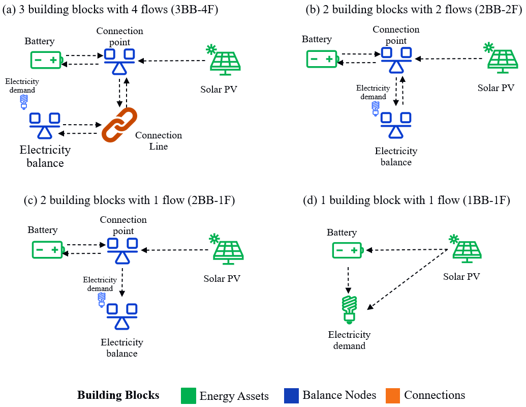
Figure 1: Using different BB to model a hybrid solar PV with storage. In general, every arrow represents one variable, and every energy asset one constraint

3.1 Three building blocks with four flow variables (3BB-4F)

This approach uses three BB: energy assets, balance nodes, and connections to link the nodes. In addition, the connection uses four positive variables to link the nodes, two for each node it connects to. This approach is advantageous as it can represent situations where the incoming flow might differ from the outgoing flow, which are needed to model transport losses or gas flows with linepack. However, when modelling transportation constraints without losses or differences between the incoming and outgoing flow, it creates extra variables and constraints.

Figure 1(a) shows the battery (bt) with a renewable (pv) example for the 2BB-4F. The connection point (cp) is an auxiliary node connecting the two assets. The electricity demand (ed) is balanced in an extra node. Moreover, the maximum capacity of the flow coming from the connection line (cl) to the connection point must be zero to avoid charging the battery from the grid (i.e., electricity demand balance node). Therefore, we need 8 variables (7 flow variables $f$ + 1 storage level $s$) and 11 constraints (8 capacity limits + 2 node balances + 1 storage balance).

• Connection point node balance constraint:

  $$f_{\text{bt,cp}}+f_{\text{pv,cp}}+f_{\text{cl,cp}}=f_{\text{cp,bt}}+f_{\text{cp,cl}}$$

• Electricity demand node balance constraint:

  $$f_{\text{cl,ed}}=D_{\text{ed}}+f_{\text{ed,cl}}$$

• Battery storage balance constraint:

  $$s_{\text{bt}}=S^{0}_{\text{bt}}+\eta^{\text{in}}_{\text{bt}}\cdot f_{\text{cp,bt}}-\frac{1}{\eta^{\text{out}}_{\text{bt}}}\cdot f_{\text{bt,cp}}$$

• Capacity limit constraints:

  $$f_{\text{bt,cp}}\leq F^{\text{max}}_{\text{bt,cp}},\quad\quad f_{\text{pv,cp}}\leq F^{\text{max}}_{\text{pv,cp}},\quad\quad f_{\text{cl,cp}}\leq F^{\text{max}}_{\text{cl,cp}},$$

  $$f_{\text{cp,bt}}\leq F^{\text{max}}_{\text{cp,bt}},\quad\quad f_{\text{cp,cl}}\leq F^{\text{max}}_{\text{cp,cl}},\quad\quad f_{\text{cl,ed}}\leq F^{\text{max}}_{\text{cl,ed}},$$

  $$f_{\text{ed,cl}}\leq F^{\text{max}}_{\text{ed,cl}},\quad\quad s_{\text{bt}}\leq S^{\text{max}}_{\text{bt}}\quad\quad$$

Where:

• $f_{\text{bt,cp}}$: flow from the battery to the connection point (i.e., battery discharge) with a maximum capacity $F^{\text{max}}_{\text{bt,cp}}$

• $f_{\text{cp,bt}}$: flow from the connection point to the battery (i.e., battery charge) with a maximum capacity $F^{\text{max}}_{\text{cp,bt}}$

• $f_{\text{pv,cp}}$: flow from the solar pv to the connection point with a maximum capacity $F^{\text{max}}_{\text{pv,cp}}$

• $f_{\text{cl,cp}}$: flow from the connection line to the connection point with a maximum capacity $F^{\text{max}}_{\text{cl,cp}}$

• $f_{\text{cp,cl}}$: flow from the connection point to the connection line with a maximum capacity $F^{\text{max}}_{\text{cp,cl}}$

• $f_{\text{cl,ed}}$: flow from the connection line to the electricity demand balance with a maximum capacity $F^{\text{max}}_{\text{cl,ed}}$

• $f_{\text{ed,cl}}$: flow from the electricity demand balance to the connection line with a maximum capacity $F^{\text{max}}_{\text{ed,cl}}$

• $s_{\text{bt}}$: storage level of the battery with a maximum capacity $S^{\text{max}}_{\text{bt}}$

• $D_{\text{ed}}$: electricity demand input data

• $\eta^{\text{in}}_{\text{bt}}$ and $\eta^{\text{out}}_{\text{bt}}$: charging and discharging efficiencies of the battery

• $S^{0}_{\text{bt}}$: initial storage level of the battery

3.2 Two building blocks with two flow variables (2BB-2F)

This approach uses as building blocks the energy assets and the balance nodes. In addition, it uses two positive flow variables to connect the nodes instead of the four variables used in the previous approach. The two flow variables are needed to model transport losses. However, gas flows with linepack cannot be modelled correctly with only two flow variables. Depending on the input data, the incoming and outgoing flow can have values simultaneously, especially when losses are not considered. In such cases, modellers typically use the net value as the transfer between the nodes. Alternatively, they may include a binary variable to prevent simultaneous incoming and outgoing flows, although this would convert the problem into a Mixed-Integer Programming problem.

Figure 1(b) shows the battery with a renewable example for the 2BB-2F. The connection point is an auxiliary node connecting the two assets. Moreover, the maximum capacity of the flow coming from the electricity balance node to the connection point must be zero to avoid charging the battery from the grid. Therefore, we need 6 variables (5 flow variables + 1 storage level) and 9 constraints (6 capacity limits + 2 node balances + 1 storage balance).

• Connection point node balance constraint:

  $$f_{\text{bt,cp}}+f_{\text{pv,cp}}+f_{\text{ed,cp}}=f_{\text{cp,bt}}+f_{\text{cp,ed}}$$

• Electricity demand node balance constraint:

  $$f_{\text{cp,ed}}=D_{\text{ed}}+f_{\text{ed,cp}}$$

• Battery storage balance constraint:

  $$s_{\text{bt}}=S^{0}_{\text{bt}}+\eta^{\text{in}}_{\text{bt}}\cdot f_{\text{cp,bt}}-\frac{1}{\eta^{\text{out}}_{\text{bt}}}\cdot f_{\text{bt,cp}}$$

• Capacity limit constraints:

  $$f_{\text{bt,cp}}\leq F^{\text{max}}_{\text{bt,cp}},\quad\quad f_{\text{pv,cp}}\leq F^{\text{max}}_{\text{pv,cp}},\quad\quad f_{\text{ed,cp}}\leq F^{\text{max}}_{\text{ed,cp}},$$

  $$f_{\text{cp,bt}}\leq F^{\text{max}}_{\text{cp,bt}},\quad\quad f_{\text{cp,ed}}\leq F^{\text{max}}_{\text{cp,ed}},\quad\quad s_{\text{bt}}\leq S^{\text{max}}_{\text{bt}}\quad\quad$$

Where the new variables are:

• $f_{\text{cp,ed}}$: flow from the connection point to the electricity demand balance with a maximum capacity $F^{\text{max}}_{\text{cp,ed}}$

• $f_{\text{ed,cp}}$: flow from the electricity demand balance to the connection point with a maximum capacity $F^{\text{max}}_{\text{ed,cp}}$

3.3 Two building blocks with one flow variable (2BB-1F)

This approach uses as building blocks the energy assets and the balance nodes. in addition, it uses a single free variable to represent the flow between nodes, which can take positive and negative values, instead of two positive variables as in the previous approach. The main advantage of this method is that it eliminates the possibility of bidirectional flow between two nodes, as there is only one variable. However, it is not possible to model transport losses using a single free variable for the flow. Lastly, the free variable must have bounds in both directions to represent the capacity limits between the two nodes.

Figure 1(c) shows the battery with a renewable example for this approach. The connection point is an auxiliary node connecting the two assets. Moreover, the maximum capacity of the flow in the direction from the electricity balance node to the connection point must be zero to avoid charging the battery from the grid. Therefore, we need 5 variables (4 flow variables + 1 storage level) and 9 constraints (6 capacity limits + 2 node balances + 1 storage balance).

• Connection point node balance constraint:

  $$f_{\text{bt,cp}}+f_{\text{pv,cp}}=f_{\text{cp,bt}}+f_{\text{cp,ed}}$$

• Electricity demand node balance constraint:

  $$f_{\text{cp,ed}}=D_{\text{ed}}$$

• Battery storage balance constraint:

  $$s_{\text{bt}}=S^{0}_{\text{bt}}+\eta^{\text{in}}_{\text{bt}}\cdot f_{\text{cp,bt}}-\frac{1}{\eta^{\text{out}}_{\text{bt}}}\cdot f_{\text{bt,cp}}$$

• Capacity limit constraints:

  $$f_{\text{bt,cp}}\leq F^{\text{max}}_{\text{bt,cp}},\quad\quad f_{\text{pv,cp}}\leq F^{\text{max}}_{\text{pv,cp}},\quad\quad f_{\text{cp,bt}}\leq F^{\text{max}}_{\text{cp,bt}},$$

  $$-F^{\text{max}}_{\text{ed,cp}}\leq f_{\text{cp,ed}}\leq F^{\text{max}}_{\text{cp,ed}},\quad\quad s_{\text{bt}}\leq S^{\text{max}}_{\text{bt}}\quad\quad$$

3.4 One building block with one flow variable (1BB-1F)

This proposed approach only uses as building blocks the energy assets. Taking advantage of the graph-theory principles establishes the connection between energy assets as vertices and energy flows as edges. Connecting assets directly to each other (without any intervening nodes) can significantly reduce the number of variables and constraints required to represent the system. When transport losses are relevant, conversion assets with efficient input-output ratios can be used to represent them. A similar approach can be adopted for gas pressure flows. Therefore, this method enables us to easily model simple and complex situations, reducing the model size while retaining the same accuracy.

Figure 1(d) shows the battery with a renewable example for the proposed 1BB-1F. Since the assets can connect among them, the battery can directly charge from renewable, and there is no need for an extra constraint to avoid charging from the grid. Therefore, we need 4 variables (3 flow variables + 1 storage level) and 6 constraints (4 capacity limits + 1 demand balance + 1 storage balance).

• Electricity demand node balance constraint:

  $$f_{\text{bt,ed}}+f_{\text{pv,ed}}=D_{\text{ed}}$$

• Battery storage balance constraint:

  $$s_{\text{bt}}=S^{0}_{\text{bt}}+\eta^{\text{in}}_{\text{bt}}\cdot f_{\text{pv,bt}}-\frac{1}{\eta^{\text{out}}_{\text{bt}}}\cdot f_{\text{bt,ed}}$$

• Capacity limit constraints:

  $$f_{\text{bt,ed}}\leq F^{\text{max}}_{\text{bt,ed}},\quad\quad f_{\text{pv,bt}}\leq F^{\text{max}}_{\text{pv,bt}},\quad\quad f_{\text{pv,ed}}\leq F^{\text{max}}_{\text{pv,ed}},$$

  $$s_{\text{bt}}\leq S^{\text{max}}_{\text{bt}}\quad\quad$$

Where the new variables are:

• $f_{\text{bt,ed}}$: flow from the battery to the electricity demand balance with a maximum capacity $F^{\text{max}}_{\text{bt,ed}}$

• $f_{\text{pv,bt}}$: flow from the solar pv to the battery with a maximum capacity $F^{\text{max}}_{\text{pv,bt}}$

• $f_{\text{pv,ed}}$: flow from the solar pv to the electricity demand balance with a maximum capacity $F^{\text{max}}_{\text{pv,ed}}$

3.5 Summary

Table 1 summarises the number of variables and constraints per time step for each modelling approach in the example shown in Figure 1. It also shows the reduction in the number of variables and constraints, with the 3BB-4F approach as a reference.

Reducing the number of variables and constraints significantly benefits the time taken to build and solve an optimisation problem, as we show in Section 5. Although the solvers’ presolve can eliminate unnecessary variables and constraints, we show that modellers can further improve this process by using formulations with fewer variables and constraints while representing the same energy system. Thus speeding up solving times.

Table 1: Number of variables and constraints in each modelling approach per time step

Modelling Approach	Variables	Constraints	Nonzeros
3BB-4F	8	11	18
2BB-2F	6 ($\downarrow$ 25%)	9 ($\downarrow$ 18%)	16 ($\downarrow$ 11%)
2BB-1F	5 ($\downarrow$ 38%)	9 ($\downarrow$ 18%)	13 ($\downarrow$ 28%)
1BB-1F	4 ($\downarrow$ 50%)	6 ($\downarrow$ 45%)	9 ($\downarrow$ 50%)

4 Calculation

The following sections describe the energy system optimisation model and a case study that compares different approaches. For the optimisation model, we have selected TulipaEnergyModel.jl [13] as it can model all the approaches based on the input data. The case study highlights situations where the 1BB-1F approach can leverage its flexibility to connect energy assets; nevertheless, Section 5.3 discusses when this is possible and provides some insights for energy system modellers.

4.1 Energy system optimisation model

TulipaEnergyModel.jl is an optimisation model using 1BB-1F and determines the optimal investment and operation decisions for different types of assets (e.g., producers, consumers, conversion, storage, and transport). It is developed in Julia [14] and depends mainly on the JuMP.jl [15] and Graphs.jl [16] packages.

The complete description of the model, its core concepts, mathematical formulation, and tutorials are available in the GitHub documentation of the model .

4.2 Case study

In our case study, we conducted experiments on three approaches: 2BB-2F, 2BB-1F, and 1BB-1F. We omitted the 3BB-4F approach because the results in Section 5 showed it would have performed worse than the other approaches for the case study. Our focus is on illustrating the performance differences between the three selected approaches.

Figure 2 shows an illustrative integrated energy system with three interconnected areas named Asgard, Midgard, and Valhalla. The diagram uses the 2BB-2F approach. In addition, it includes the flow and balance of electricity, heat, and gas within a mock-up energy grid to explore different possibilities for flows among energy assets using nodes. Asgard includes a combined cycle gas turbine, a solar photovoltaic installation, and a battery system. Midgard features a wind park, a hydro plant, and a small modular reactor for nuclear power generation. Valhalla focuses on hydrogen as an energy vector, with a hydrogen generator, a hydrogen storage facility, and a fuel cell. Transmission lines and gas pipelines connect the system, allowing energy transfer between areas.

Figures 3 and 4 show the equivalent energy system for the other two approaches. In general, each arrow represent a variable and each BB element represents a constraint. Note that the number of flows (arrows) reduces compared to the 2BB-2F approach. For the purpose of evaluating the impact of different problem sizes, we created six instances of the problem, ranging from small to large-scale optimisation, with the smallest being labelled as 1 and the largest as 6. Section 5 analyses the impact of these reductions in the model for each approach and instance. Finally, Section 9 has the link to the repository with the input data files for each approach.

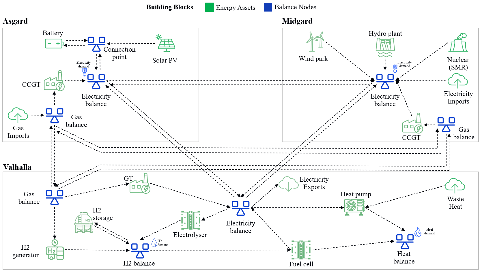
Figure 2: Case study using 2BB-2F

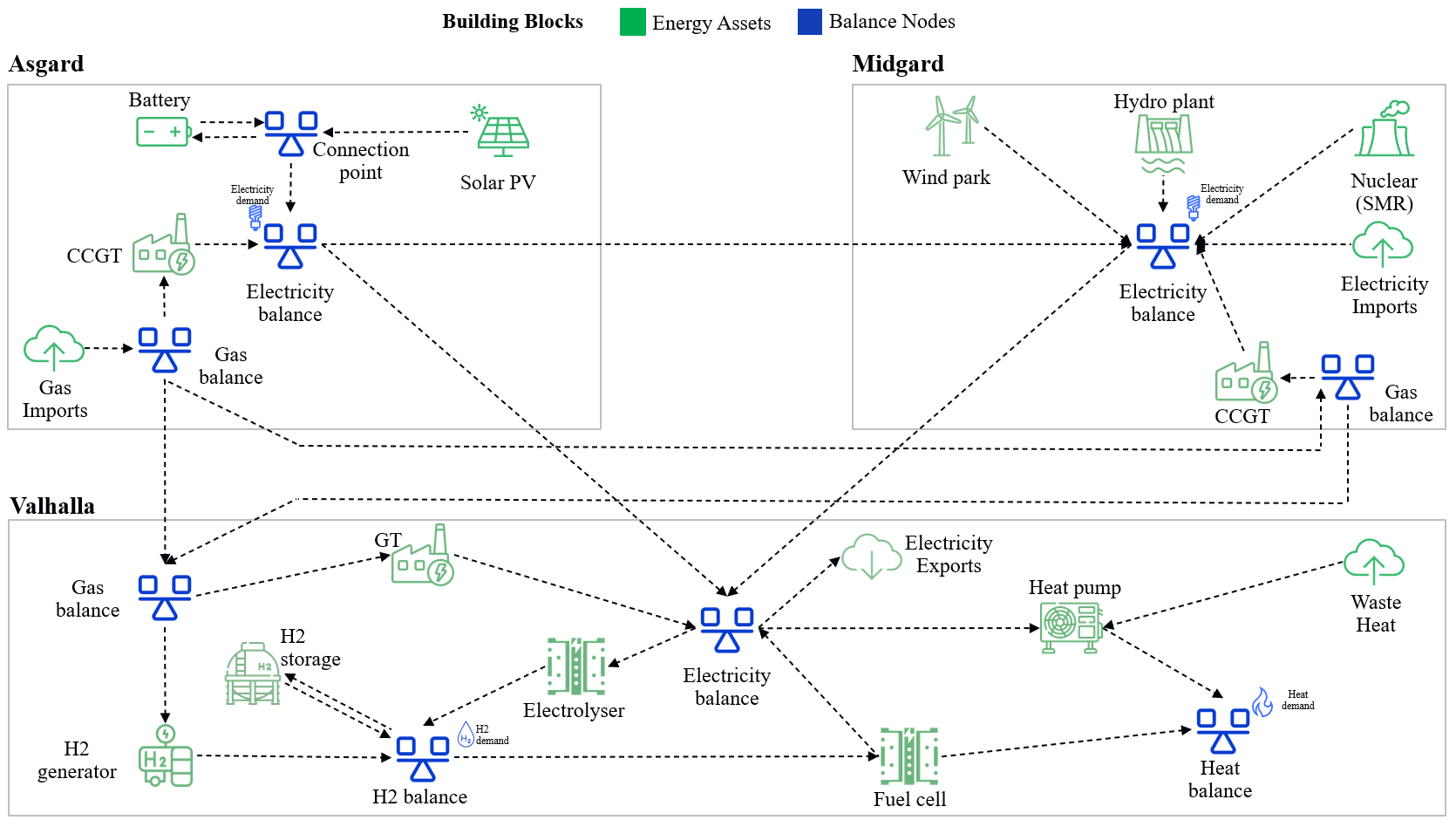
Figure 3: Case study using 2BB-1F

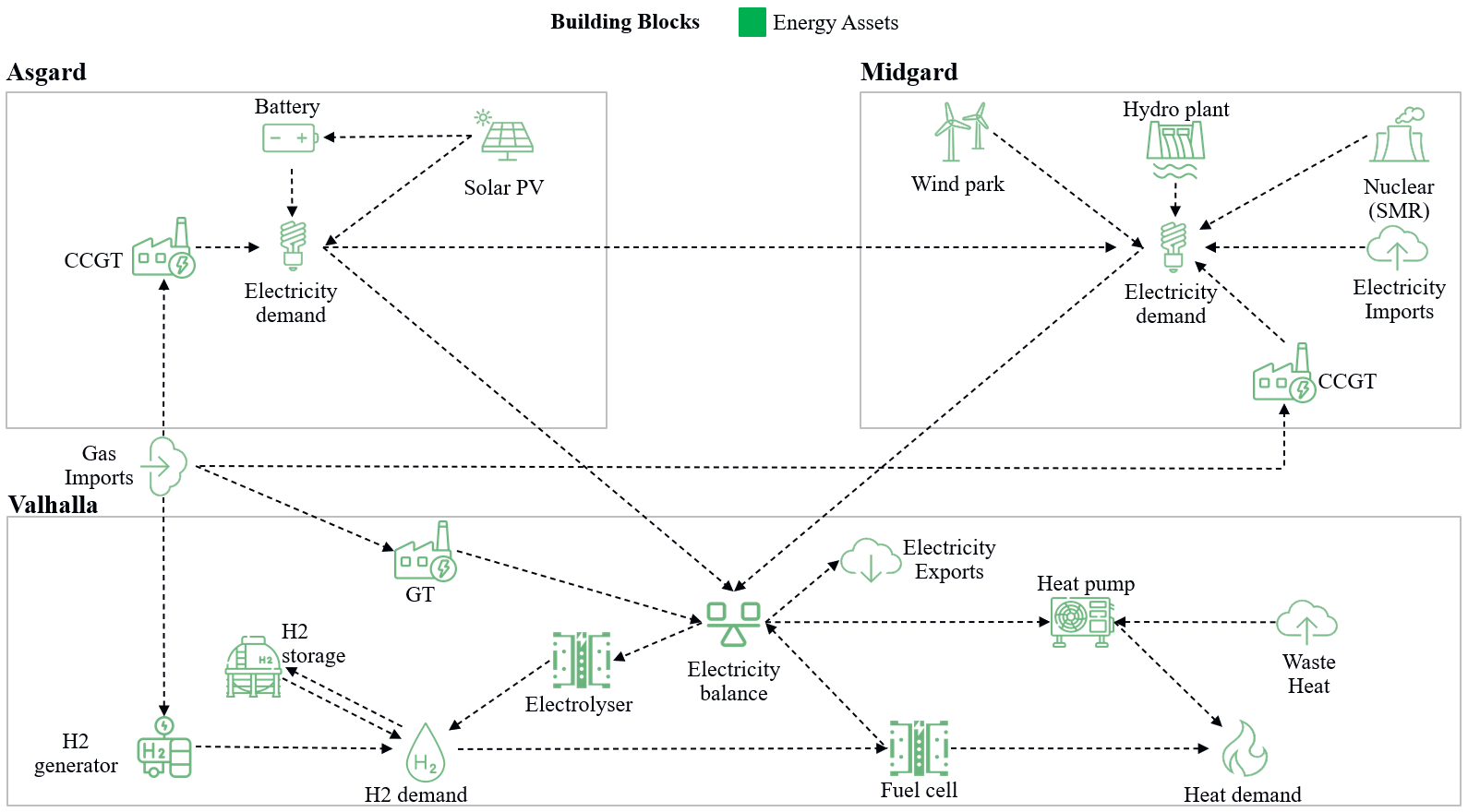
Figure 4: Case study using 1BB-1F

5 Results

The results in this section were obtained using TulipaEnergyModel.jl version 0.6.1 and Gurobi version 11.0.0 on a 12th Gen Intel(R) Core(TM) i7-1255U 1.70 GHz processor, and 16.0 GB RAM. Section 9 includes the link to the repository with the files to reproduce the experiments in this paper.

Table 2 shows the objective functions and problem size for each instance, where 2BB-2F is used as a reference in the table. The reduction in the number of variables and constraints is 14% and 18% for the 2BB-1F approach and 26% and 35% for the 1BB-1F approach. It is important to highlight that the reduction is identical for all instances since the instance is an enlarged version of the same case study. Still, the connection between assets remains unchanged in all instances. It is also worth noting that the objective function is the same for every instance, regardless of the applied approach, indicating that they all represent the same energy problem. Finally, we cover a wide range of model sizes, from smaller instances representing optimisation models with a few thousand variables and constraints to larger instances with millions of variables and constraints.

Table 2: Size of the problem in each modelling approach

Approach	Instance	Obj. func	Variables	Constraints	Nonzeros
	1	2.48E+08	28,908	45,696	96,318
	2	3.55E+08	173,388	274,176	578,609
2BB-2F	3	6.10E+08	376,692	595,680	1,257,055
	4	1.05E+09	753,372	1,191,360	2,514,096
	5	1.48E+09	1,130,052	1,787,040	3,771,168
	6	1.89E+09	1,506,732	2,382,720	5,028,256
2BB-1F	1-6	1 p.u.	$\downarrow 14\%$	$\downarrow 18\%$	$\downarrow 17\%$
1BB-1F	1-6	1 p.u.	$\downarrow 26\%$	$\downarrow 35\%$	$\downarrow 29\%$

The graph in Figure 5 depicts the median speedup values for building and solving models using the three approaches and all the instances. The reference point used for comparison is the 2BB-2F approach. The values for the other approaches indicate the proportion of time the approach takes compared to the reference one. Reducing the number of variables and constraints has advantageous effects on building and solving models. Creating fewer variables and constraints has a significant advantage when building the model. Interestingly, there is a trend towards greater speedups as the instances increase. The surprising result is that having fewer variables and constraints also leads to speedups in the solving phase, with a slight trend towards increasing speedups as the instance size grows. Solvers can leverage these reductions to solve the model faster at each iteration with fewer variables and constraints. It is common practice among energy modellers to rely on the solver’s presolve function to eliminate redundant variables and constraints. However, having a clean and concise formulation representing the same energy problem is always better, as it allows the solver to be faster in its process.

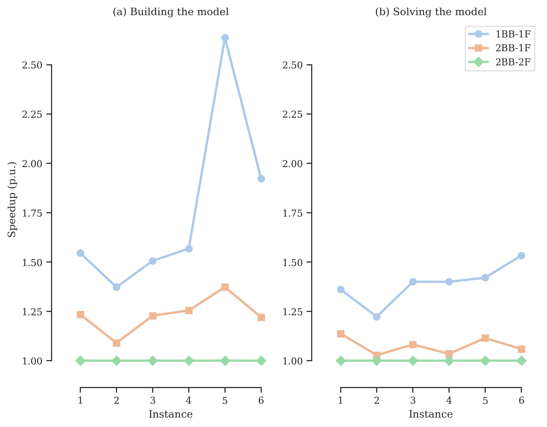
Figure 5: Speedups comparison

5.1 Sensitivity analysis

It is important to comment that commercial optimisation solvers, such as Gurobi, can yield different results based on the ”seed” parameter used [17]. Therefore, relying on a single run is not the best procedure for comparing different modelling approaches. Furthermore, the time it takes to build the model can vary due to random variations in CPU processing, which can also lead to differences between each run. To address this, we conducted a sensitivity analysis with 30 different seeds for each approach and optimisation instance, calculating median values for each group to determine if there are any statistically significant differences. We chose the median value as it is a central measure unaffected by data outliers. Figure 6 shows the distribution of speedups and their means with the 2BB-2F approach as a reference for all results in each instance. Similarly, Figure 7 shows the results for solving time. Both figures suggest a difference between the 1BB-1F approach and both approaches using two building blocks, i.e., 2BB-2F and 2BB-1F. However, the 2BB-2F and 2BB-1F approaches are closer in the distribution of values. Section 5.2 provides a statistical analysis of the results to determine if there’s enough statistical evidence to support these hypotheses.

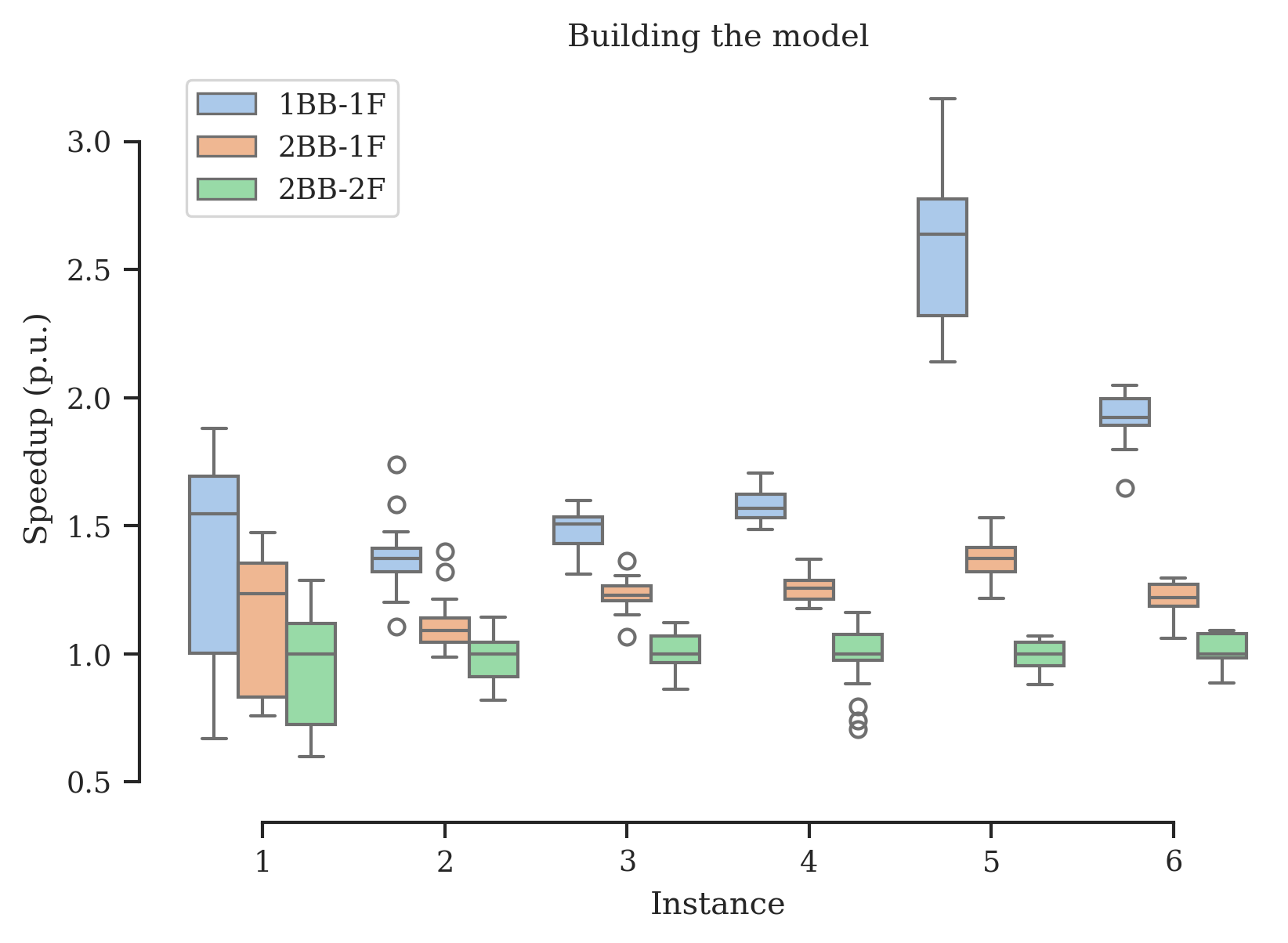
Figure 6: Speedups distribution comparison for the time to build

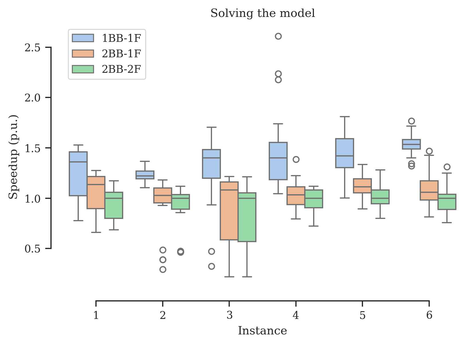
Figure 7: Speedups distribution comparison for the total time to solve

5.2 Statistical analysis

To determine if there is a significant difference between the modelling approaches, we use a two-sample t-test. The null hypothesis states that the average values of two related or repeated samples are identical. In contrast, the alternative hypothesis suggests that the underlying distributions of the samples have unequal means.

The randomness in the results is due to the random number seed in the solver, which leads the solver to take different solution paths. Therefore, we can assume for the t-test that the results follow a normal probability distribution, the variances of the results are equal, and each individual in the population has an equal probability of being selected in the sample.

We use 2BB-2F as the reference and compare it individually with 2BB-1F and 1BB-1F. Here, we assume a significance level of $\alpha=0.05$. Table 3 shows the test results for each instance and compared approach. If the p-value is smaller than the threshold, we reject the null hypothesis of equal averages. Then, there is a statistically significant difference between the mean times of 2BB-2F and the others (2BB-1F and 1BB-1F).

The results presented in Table 3 indicate that 1BB-1F has a significantly different mean value than 2BB-2F in all instances. Additionally, Figure 7 shows that the average speedup values are higher for 1BB-1F in all cases. This implies that while 2BB-2F could potentially be faster than 1BB-1F in a particular instance, there is statistical evidence that, on average, 1BB-1F is faster. As for 2BB-1F, no statistical evidence suggests that it is faster than 2BB-F for half of the instances. However, it is worth noting that the larger case studies in the test, instances 5 and 6, show statistical evidence that the 2BB-1F approach is faster, on average, than the 2BB-2F.

We are left with the question of how the 1BB-1F approach compares to the 2BB-1F approach. We also use a two-sample t-test with the 2BB-1F approach as the reference to compare these approaches. The results in Table 4 indicate that the 1BB-1F approach is statistically faster for all instances, as shown in Figure 7.

Table 3: T-test results using 2BB-2F as reference

Compared Approach	Instance	t-statistic	p-value
	1	2.11	0.04
	2	-0.37	0.72
2BB-1F	3	0.34	0.74
	4	1.74	0.09
	5	4.47	0.00
	6	2.60	0.01
	1	6.68	0.00
	2	4.83	0.00
1BB-1F	3	4.78	0.00
	4	9.49	0.00
	5	11.48	0.00
	6	15.08	0.00

Table 4: T-test results using 2BB-1F as reference

Compared Approach	Instance	t-statistic	p-value
	1	6.68	0.00
	2	4.83	0.00
1BB-1F	3	4.78	0.00
	4	9.49	0.00
	5	11.48	0.00
	6	15.08	0.00

5.3 Discussion

Nowadays, energy system modellers have access to several energy models that can be used to develop case studies. These models can have one or more available modelling options that can be framed in different approaches, which are described in this paper. Table 5 provides a general overview of the main available modelling approaches in a sample of energy system models. Models focusing on power systems mainly consist of two building blocks, nodes and energy assets. In contrast, most recent models that focus on multi-sector analysis, like Calliope and SpineOpt, have three building blocks: nodes, energy assets, and connections. The reason behind having more building blocks is to create a flexible model that can adapt to different energy asset configurations and represent different sectors. However, a flexible model can result in an increase in the number of variables and constraints, which can come with a computation cost. The results in the illustrative example in this paper estimate the impact in terms of speedup. As a general recommendation for energy system modellers, it is better to have fewer variables, especially for large-scale case studies.

In order to reduce the size of the model, instead of reformulating the model using a single building block as proposed in this paper, some models provide the option to select specific methods tailored to the application. These methods also aim to reduce the number of variables and constraints. For instance, IRENA FlexTool gives users a selection of conversion and transfer methods, and some of those methods allow the use of fewer variables and constraints when the model is created, which also improves the solution process in the solver. FlexTool can actually present the example problem in 1BB-1F format with one extra variable using available methods and in full 1BB-1F format using carefully formulated user constraints, which can be entered as data. In both cases, the benefit comes from choosing a modelling approach or method with fewer variables and constraints to represent the same energy system. The advantage of the 1BB-1F proposal in this paper is that it is a generic way to formulate the problem without depending on the definition of tailor-made methods for each case.

The proposal for using only one building block with one flow variable (1BB-1F) is a new way of utilizing the network graph structure of energy systems. While this approach has been found to offer several advantages, it also poses two primary challenges. First and foremost, it involves an extra layer of abstraction as the proposal can establish direct connections between energy assets, which may not be very intuitive compared to traditional methods that use more building blocks like nodes and connections. However, this level of abstraction does not hinder the modellers from representing assets that perform the functions of nodes or connections, as evidenced in the case study where the same model, TulipaEnergyModel, was utilized to represent all the modelling approaches. Secondly, it is not always possible to obtain the benefits of asset-to-asset connections (1BB-1F) in situations where gas pressure constraints, transport delays, or DCOPF losses are considered. Modelling these situations results in variations between an energy asset’s incoming and outgoing flows, which reduces or eliminates the potential reduction on the model size of the 1BB-1F approach. In such cases, it becomes necessary to include two or four flow variables to represent the situation accurately. So, the 1BB-1F is not a silver bullet, but it can help in large-scale optimisation problems that can be simplified.

Table 5: Overview of available modelling approaches in a sample of energy system models

Model	Main focus	Year	Approach
Backbone [18]	Multi-sector	2016	2BB-1F
Calliope [19]	Multi-sector	2018	3BB-4F
COMPETES [20]	Power Systems	2004	2BB-2F
FlexTool [6]	Power Systems	2021	2BB-1F
GenX [21]	Power Systems	2022	2BB-1F
OSEMOSYS [12]	Multi-sector	2016	2BB-2F
PowerSystems [22]	Power Systems	2021	2BB-1F
PyPSA [11]	Power Systems	2018	2BB-1F
SpineOpt [7]	Multi-sector	2022	3BB-4F
TIMES [23]	Multi-sector	2016	2BB-2F
TulipaEnergyModel [13]	Multi-sector	2023	1BB-1F

6 Conclusion

Representing the same energy system in optimisation models with fewer variables and constraints without compromising accuracy is possible. Modellers must understand the impact of their choices on the model’s performance since flexible models allow for different approaches. This research has debunked the idea that an LP model’s simplicity cannot be improved without sacrificing fidelity and highlighted the importance of carefully considering different approaches representing energy system interactions. The extended concept of a network graph has shown great potential in reducing the number of variables and constraints in the model by using only one building block (1BB-1F). It can speed up the time required to create and solve the model by an average of 1.76 and 1.27, respectively, across all the case study instances. Notably, these benefits increase with the size of the problem, making it particularly advantageous for large-scale problems.

We hope this analysis will raise awareness in the modelling community about the importance of making conscious decisions when representing energy systems. This analysis could be expanded to cover a wider range of physical dynamics of energy systems and their synergies with other commonly used reduction techniques in the literature.

7 CRediT author statement

Diego A. Tejada-Arango: Methodology, Writing- Original draft preparation, Formal analysis, Software. Germán Morales-España: Methodology, Validation, Writing- Reviewing and Editing, Funding acquisition. Juha Kiviluoma: Conceptualization, Writing- Reviewing and Editing, Funding acquisition.

8 Acknowledgments

This research received funding from the European Climate, Infrastructure and Environment Executive Agency under the European Union’s HORIZON Research and Innovation Actions under grant agreement N°101095998. In addition, the Dutch Research Council (NWO) also partially funded this research under grant number ESI.2019.008.

Disclaimer: Views and opinions expressed are those of the author(s) only and those of the European Union or NWO. Neither the European Union nor the granting authority can be held responsible.

9 Supplementary material

All the code to run the experiments and the raw results in this paper are available at the following link:

https://github.com/datejada/experiments-flexible-connection

References

- TNO [2020] TNO, Energy system description language, 2020. URL: https://energytransition.gitbook.io/esdl/esdl-concepts/design-principles, accessed on March 19th, 2024.
- Wiese et al. [2018] F. Wiese, R. Bramstoft, H. Koduvere, A. Pizarro Alonso, O. Balyk, J. G. Kirkerud, Åsa Grytli Tveten, T. F. Bolkesjø, M. Münster, H. Ravn, Balmorel open source energy system model, Energy Strategy Reviews 20 (2018) 26–34. URL: https://www.sciencedirect.com/science/article/pii/S2211467X18300038. doi:https://doi.org/10.1016/j.esr.2018.01.003.
- Energy Exemplar [2000] Energy Exemplar, Plexos, 2000. URL: https://www.energyexemplar.com/plexos, accessed on March 11th, 2024.
- Morales-España et al. [2024] G. Morales-España, R. Hernández-Serna, D. A. Tejada-Arango, M. Weeda, Impact of large-scale hydrogen electrification and retrofitting of natural gas infrastructure on the european power system, International Journal of Electrical Power & Energy Systems 155 (2024) 109686. URL: https://www.sciencedirect.com/science/article/pii/S0142061523007433. doi:https://doi.org/10.1016/j.ijepes.2023.109686.
- Gea-Bermúdez et al. [2021] J. Gea-Bermúdez, I. G. Jensen, M. Münster, M. Koivisto, J. G. Kirkerud, Y. kuang Chen, H. Ravn, The role of sector coupling in the green transition: A least-cost energy system development in northern-central europe towards 2050, Applied Energy 289 (2021) 116685. URL: https://www.sciencedirect.com/science/article/pii/S0306261921002130. doi:https://doi.org/10.1016/j.apenergy.2021.116685.
- Kiviluoma et al. [2022] J. Kiviluoma, A. Tupala, A. Soininen, International Renewable Energy Agency (IRENA), IRENA FlexTool, 2022. URL: https://github.com/irena-flextool/flextool.
- Ihlemann et al. [2022] M. Ihlemann, I. Kouveliotis-Lysikatos, J. Huang, J. Dillon, C. O’Dwyer, T. Rasku, M. Marin, K. Poncelet, J. Kiviluoma, Spineopt: A flexible open-source energy system modelling framework, Energy Strategy Reviews 43 (2022) 100902. URL: https://www.sciencedirect.com/science/article/pii/S2211467X22000955. doi:https://doi.org/10.1016/j.esr.2022.100902.
- Markensteijn et al. [2020] A. Markensteijn, J. Romate, C. Vuik, A graph-based model framework for steady-state load flow problems of general multi-carrier energy systems, Applied Energy 280 (2020) 115286. URL: https://www.sciencedirect.com/science/article/pii/S0306261920307984. doi:https://doi.org/10.1016/j.apenergy.2020.115286.
- Klotz and Newman [2013] E. Klotz, A. M. Newman, Practical guidelines for solving difficult linear programs, Surveys in Operations Research and Management Science 18 (2013) 1–17. URL: https://www.sciencedirect.com/science/article/pii/S1876735412000189. doi:https://doi.org/10.1016/j.sorms.2012.11.001.
- Lustig et al. [1991] I. J. Lustig, J. M. Mulvey, T. J. Carpenter, Formulating two-stage stochastic programs for interior point methods, Operations Research 39 (1991) 757–770. URL: https://doi.org/10.1287/opre.39.5.757. doi:10.1287/opre.39.5.757. arXiv:https://doi.org/10.1287/opre.39.5.757.
- Brown et al. [2018] T. Brown, J. Hörsch, D. Schlachtberger, PyPSA: Python for Power System Analysis, Journal of Open Research Software 6 (2018). URL: https://doi.org/10.5334/jors.188. doi:10.5334/jors.188. arXiv:1707.09913.
- Howells et al. [2011] M. Howells, H. Rogner, N. Strachan, C. Heaps, H. Huntington, S. Kypreos, A. Hughes, S. Silveira, J. DeCarolis, M. Bazillian, A. Roehrl, Osemosys: The open source energy modeling system: An introduction to its ethos, structure and development, Energy Policy 39 (2011) 5850–5870. URL: https://www.sciencedirect.com/science/article/pii/S0301421511004897. doi:https://doi.org/10.1016/j.enpol.2011.06.033, sustainability of biofuels.
- Tejada-Arango et al. [2023] D. A. Tejada-Arango, G. Morales-España, L. Clisby, N. Wang, A. Soares Siqueira, S. Ali, L. Soucasse, G. Neustroev, Tulipa Energy Model, 2023. URL: https://github.com/TulipaEnergy/TulipaEnergyModel.jl.
- Bezanson et al. [2017] J. Bezanson, A. Edelman, S. Karpinski, V. B. Shah, Julia: A fresh approach to numerical computing, SIAM Review 59 (2017) 65–98. doi:10.1137/141000671.
- Lubin et al. [2023] M. Lubin, O. Dowson, J. Dias Garcia, J. Huchette, B. Legat, J. P. Vielma, JuMP 1.0: Recent improvements to a modeling language for mathematical optimization, Mathematical Programming Computation (2023). doi:10.1007/s12532-023-00239-3.
- Fairbanks et al. [2021] J. Fairbanks, M. Besançon, S. Simon, J. Hoffiman, N. Eubank, S. Karpinski, Juliagraphs/graphs.jl: an optimized graphs package for the julia programming language, 2021. URL: https://github.com/JuliaGraphs/Graphs.jl/.
- Tejada-Arango et al. [2020] D. A. Tejada-Arango, S. Lumbreras, P. Sánchez-Martín, A. Ramos, Which unit-commitment formulation is best? a comparison framework, IEEE Transactions on Power Systems 35 (2020) 2926–2936. doi:10.1109/TPWRS.2019.2962024.
- Helistö et al. [2019] N. Helistö, J. Kiviluoma, J. Ikäheimo, T. Rasku, E. Rinne, C. O’Dwyer, R. Li, D. Flynn, Backbone—an adaptable energy systems modelling framework, Energies 12 (2019). URL: https://www.mdpi.com/1996-1073/12/17/3388. doi:10.3390/en12173388.
- Pfenninger and Pickering [2018] S. Pfenninger, B. Pickering, Calliope: a multi-scale energy systems modelling framework, Journal of Open Source Software 3 (2018) 825. URL: https://doi.org/10.21105/joss.00825. doi:10.21105/joss.00825.
- Özge Özdemir et al. [2019] Özge Özdemir, B. F. Hobbs, M. van Hout, P. Koutstaal, Capacity vs energy subsidies for renewables: Benefits and costs for the 2030 eu power market, Energy Policy Research Group, University of Cambridge (2019). URL: http://www.jstor.org/stable/resrep30402.
- Jenkins et al. [2022] J. Jenkins, N. Sepulveda, D. Mallapragada, N. Patankar, A. Schwartz, J. Schwartz, S. Chakrabarti, Q. Xu, J. Morris, N. Sepulveda, GenX, 2022. URL: https://github.com/GenXProject/GenX. doi:10.5281/zenodo.6229425.
- Lara et al. [2021] J. D. Lara, C. Barrows, D. Thom, D. Krishnamurthy, D. Callaway, Powersystems.jl — a power system data management package for large scale modeling, SoftwareX 15 (2021) 100747. URL: https://www.sciencedirect.com/science/article/pii/S2352711021000765. doi:https://doi.org/10.1016/j.softx.2021.100747.
- Loulou et al. [2016] R. Loulou, G. Goldstein, A. Kanudia, A. Lettila, U. Remme, E. Wright, G. Giannakidis, K. Noble, Documentation for the TIMES Model - Part I, 2016. URL: https://iea-etsap.org/index.php/documentation.