Without Pain – Clustering Categorical Data Using a Bayesian Mixture of Finite Mixtures of Latent Class Analysis Models

We propose a Bayesian approach for model-based clustering of multivariate categorical data where variables are allowed to be associated within clusters and the number of clusters is unknown. The approach uses a two-layer mixture of finite mixtures model where the cluster distributions are approximated using latent class analysis models. A careful specification of priors with suitable hyperparameter values is crucial to identify the two-layer structure and obtain a parsimonious cluster solution. We outline the Bayesian estimation based on Markov chain Monte Carlo sampling with the telescoping sampler and describe how to obtain an identified clustering model by resolving the label switching issue. Empirical demonstrations in a simulation study using artificial data as well as a data set on low back pain indicate the good clustering performance of the proposed approach provided hyperparameters are selected that induce sufficient shrinkage.

1 Introduction

In this paper, we develop a model-based clustering approach for multivariate categorical data. All variables are assumed cluster-relevant but they are potentially associated within clusters. The approach also infers a suitable number of clusters. In particular, the motivation for developing this approach is a specific data set investigating low back pain disorders described in Fop et al. (2017). A questionnaire was developed for patients by experienced physiotherapists where the answers allow to classify patients according to the type of low back pain they are suffering from. The questionnaire consists of a range of binary questions about the presence or absence of certain pain symptoms. As the list of clinical criteria was assembled by experts, all variables are expected to possess good discriminatory power and, hence, are potentially cluster-informative. However, it is also suspected that some of the indicators carry the same information about the low back pain type, i.e., they are redundant. Additionally, variables are expected to be dependent within the low back pain types due to the same underlying neurophysiological mechanisms being responsible for the pain generation and the manifestation captured by several binary indicators. To address this association within clusters, we propose an extension of the latent class analysis model for Bayesian model-based clustering where all variables (also the “redundant” ones) are included in the analysis and where within-group associations between variables are accounted for.

Latent class analysis (LCA; Lazarsfeld, 1950; Goodman, 1974) is a well-established framework which has been developed to model dependence among multivariate categorical variables. LCA assumes that the dependency structure between categorical variables observed in the data is due to the presence of latent groups called classes and that conditional on class membership the categorical variables are independent. This model class thus represents a convenient way to capture dependencies between categorical variables. However, assuming conditionally independent variables, i.e., that classes are fully characterized by the occurrence probability of each category of a variable, is very restrictive in a clustering context. The sparsity of the model, implied by the conditionally independence assumption, is of great advantage, but in clustering applications this assumption might be questionable. In the presence of within-cluster associations, the standard LCA model will fit more classes than there are clusters in the data, in order to provide an adequate fit to the data. As a consequence, the assumption of a one-to-one relationship between the classes of the LCA model and the clusters in the data is no longer applicable, degrading the interpretability of the estimated clusters.

In the literature, approaches to account for association between categorical variables within clusters follow basically two streams of research. The first approach consists in selecting a subset of the observed variables in order to extract independent, cluster-relevant variables, see, e.g., Maugis et al. (2009); Dean and Raftery (2010); Bartolucci et al. (2016); White et al. (2016); Fop et al. (2017). The second approach consists in modeling explicitly the conditional dependencies in the classes. In log-linear models (Bock, 1986; Agresti, 2002; Papathomas and Richardson, 2016), the frequencies in the contingency table obtained by cross-tabulating the categorical variables are modeled by including suitable interaction terms between variables. Multilevel latent class models (Vermunt and Magidson, 2003) assume that the cluster-specific distribution of the categorical variables depends on continuous latent variables which allow to model the dependencies among the observed categorical variables in the latent space. Gollini and Murphy (2014) propose a mixture of latent trait analyzers to accommodate dependencies within a cluster. Marbac et al. (2015) investigate a block extension of the LCA model, where conditional on the class, the variables are grouped into independent blocks, with each block following a specific distribution which takes into account the dependency between variables.

In this work, we combine the original idea of the LCA model, namely to capture associated categorical variables by the introduction of a latent group variable, with a model-based clustering approach. We propose a mixture of LCA models which results in a two-layer model. On the upper level, the mixture approach is used for model-based clustering of the data, while on the lower level the component-specific LCA model represents a cluster in the data and is used to approximate the cluster distribution, allowing for association between variables within a cluster to be captured. On the lower level, each cluster is assumed to be composed of several classes to capture the association within variables and these classes thus do not correspond to identifiable groups. In the following we will call the (possibly associated) components of the mixture distribution on the upper level “components” or “clusters”, while the classes of the LCA models on the lower level are called “subcomponents” or “classes”.

Statistical inference of finite mixtures is generally complicated due to spurious modes and unboundedness of the mixture likelihood (see, e.g., Frühwirth-Schnatter 2006, chap. 2). But the estimation of a two-layer mixture model is particularly challenging due to its identifiability issues. Exchanging subcomponents on the lower level between components of the upper level leads to different component-specific distributions, but overall the mixture density remains the same. Thus, a two-layer mixture model is not identifiable based on the mixture likelihood alone in the absence of additional information. This is especially problematic in the context of clustering, as only identified clusters are interpretable, see a recent discussion in Gu and Dunson (2023) in the framework of deep learning models.

In the Bayesian setting, we resolve the identifiability issue of the two-layer mixture model by specifying suitable priors which favor a unique assignment of the classes in the LCA models on the lower level to components on the upper level. For a mixture of Gaussian mixtures, i.e., a two-layer mixture model for multivariate continuous data, Malsiner-Walli et al. (2017) suggested a prior which induces shrinkage of the subcomponent means on the lower level toward a cluster-specific center on the upper level to obtain identifiability. In this paper, we investigate how the approach developed for mixtures of multivariate Gaussian mixtures can be extended and adapted to mixtures of LCA models. We propose a prior specification which induces shrinkage of the subcomponent occurrence probabilities toward a central, cluster-specific occurrence probability vector. This is related to Durante et al. (2017) who, in the framework of network-valued data, define the component-specific edge-probability vector as a function of a shared similarity vector, common to all components, and a component-specific deviation vector, which is pulled toward zero by a shrinkage prior. However, in contrast to Durante et al. (2017), who operate in the underlying latent continuous space, we model the common “center” of the occurrence probabilities of the classes belonging to the same cluster and also their “precision” around the common center directly, without referring to any latent space representation.

Our proposed Bayesian mixture of LCA models approach also addresses the issue of selecting the number of clusters in the data. If the number of clusters in the data is unknown, in the Bayesian setting a prior on the number of components in the mixture distribution can be specified, and the resulting model is referred to as a “mixture of finite mixtures (MFM) model” (Miller and Harrison, 2018; Frühwirth-Schnatter et al., 2021). For a MFM model, inference is challenging as a transdimensional sampler is required which is able to jump between parameter spaces of varying dimension. We use a Gibbs sampling scheme with data augmentation for Markov chain Monte Carlo (MCMC) inference which relies on the telescoping sampler proposed by Frühwirth-Schnatter et al. (2021) as an alternative to other, more complex approaches such as Reversible Jump MCMC (Richardson and Green, 1997) or Chinese Restaurant process based sampling schemes popular in Bayesian non-parametrics (Miller and Harrison, 2018). An advantage of the telescoping sampler is that sampling of the number of components is performed conditional on the current partition of the data into non-empty clusters and completely independent of the component distributions. This makes the sampler easy to implement when fitting a Bayesian mixture of LCA models where the components are part of a multi-layer model.

The rest of the article is organized as follows. Section 2 provides the model specification including a detailed discussion of the selected priors to obtain a Bayesian mixture of LCA models suitable for clustering multivariate categorical data. Model estimation and identification are discussed in Section 3. The performance of the proposed strategy is evaluated in Section 4 in a simulation study and for the low back pain data set already used in Fop et al. (2017). Section 5 concludes.

2 Bayesian mixture of finite mixtures of latent class analysis models

2.1 Data model

We consider multivariate categorical observations $\bm{y}_{i}$, $i=1,\ldots,N$, consisting of $r$ variables where each variable $j=1,\ldots,r$ is categorical with $D_{j}$ categories. Each observation is given by $\bm{y}_{i}=(y_{ij})_{j=1,\ldots,r}$ with $y_{ij}\in\{1,\ldots,D_{j}\}$. The $N$ observations $\bm{y}_{i}$ are assumed to be generated independently from a finite mixture distribution with $K$ components with density

$$p(\bm{y}_{i}|K,\bm{\Theta}_{K},\bm{\eta}_{K}) =\sum_{k=1}^{K}\eta_{k}p_{k}(\bm{y}_{i}|\bm{\theta}_{k}),$$ (1)

where, for a fixed number of components $K$, $\bm{\Theta}_{K}=(\bm{\theta}_{k})_{k=1,\ldots,K}$ is the vector of component-specific parameters and $\bm{\eta}_{K}=(\eta_{k})_{k=1,\ldots,K}$ are the positive component weights with

$$\sum_{k=1}^{K}\eta_{k} =1.$$

Each component distribution $p_{k}(\bm{y}_{i}|\bm{\theta}_{k})$ is given by a LCA model, i.e.,

$$p_{k}(\bm{y}_{i}|\bm{\theta}_{k}) =\sum_{l=1}^{L}w_{kl}\prod_{j=1}^{r}\prod_{d=1}^{D_{j}}\pi_{kl,jd}^{I\{y_{ij}=d\}},$$ (2)

where $L$ is the number of classes (subcomponents) of component $k$ and $\bm{w}_{k}=(w_{kl})_{l=1,\ldots,L}$ are the positive subcomponent weights with

$$\sum_{l=1}^{L}w_{kl} =1.$$

Note that we assume that the number of classes (subcomponents) $L$ is the same across all components. In principle one could also specify a value $L_{k}$ which varies across components and is learned from the data.

The component-specific parameter $\bm{\theta}_{k}$ consists of $(\bm{w}_{k},\bm{\pi}_{k})$, where $\bm{\pi}_{k}=(\pi_{kl,jd})_{d=1,\ldots,D_{j};j=1,\ldots,r;l=1,\ldots,L}$ with $\pi_{kl,jd}$ equal to the occurrence probability of observation $y_{ij}$ taking category $d$ conditional on being from subcomponent $l$ of component $k$. The vector of subcomponent weights is given by $\bm{w}_{KL}=(\bm{w}_{k})_{k=1,\ldots,K}$ and the vector of subcomponent occurrence probabilities by $\bm{\pi}_{KL}=(\bm{\theta}_{k})_{k=1,\ldots,K}$.

2.2 Prior specification

The data model specified in (1) and (2) is complemented by priors for the model parameters $(K,\bm{\eta}_{K},L,\bm{w}_{KL},\bm{\pi}_{KL})$. In the following, we carefully select priors to achieve the following modeling aims: (1) estimation of a parsimonious number of clusters in the data and (2) identification of the cluster-specific distributions. We use conditionally conjugate priors, where possible, to ease inference. Further, we impose exchangeable priors across the components and subcomponents to preserve prior invariance and symmetry with respect to arranging the components in a mixture distribution.

2.2.1 Determining the number of components and subcomponents

In clustering applications, the number of components $K$ in the upper level model (1) is usually not known. In the Bayesian framework, it is natural to treat $K$ as a random variable and to specify a prior on it, i.e.,

$$K \sim p(K).$$

This results in a mixture of finite mixtures model (MFM; Miller and Harrison, 2018) and posterior inference for $K$ can be employed to determine a suitable number of components.

Frühwirth-Schnatter et al. (2021) review previous suggestions for the prior on $K$ and propose to use the shifted beta-negative-binomial (BNB) distribution for $K$. This distribution encompasses other distributions previously proposed as special cases (i.e., the Poisson, the geometric and the negative-binomial distribution). The shifted BNB distribution is a three-parameter distribution which allows to not only to calibrate the prior mean and variance, but also to control separately the probability of the homogeneity model $K=1$ and the tail behavior, i.e., the mass assigned to large values of $K$. Following Frühwirth-Schnatter et al. (2021) and Grün et al. (2022), we propose to use $K-1\sim\mathit{BNB}(1,4,3)$ as a suitable prior on $K$ in a clustering application. This prior concentrates a lot of mass on the homogeneity model and assigns decreasing prior weights to increasing number of components, while still having some mass assigned to larger values. See Appendix A for more details on the BNB distribution.

On the lower level, also the number of classes is typically unknown for each component $k$. However, on this level we are not interested in estimating the “true” number of classes forming cluster $k$, as there is no clustering task on this level. We only need to ensure that this number is chosen sufficiently large to be flexible enough to capture the association structure in cluster $k$. Similar to kernel density estimation, where the exact number of kernels is usually not of interest as long as the approximation is sufficiently close, we select a fixed, sufficiently large value $L$ for the number of classes across all components. However, a too generous choice of $L$ should be avoided for computational reasons. In our analyses we set $L$ to a fixed value varying between $2$ and $5$ which is sufficient to capture the within-cluster associations in our applications.

The priors on the component weights $\bm{\eta}_{K}$ on the upper level as well as the subcomponent weights $\bm{w}_{k}$, $k=1,\ldots,K$, on the lower level are specified by symmetric Dirichlet distributions with parameters $\gamma_{K}$ and $\delta$, respectively:

$$\bm{\eta}_{K}|K \sim\mathcal{D}_{K}(\gamma_{K}), \bm{w}_{k} \sim\mathcal{D}_{L}(\delta),\quad k=1,\ldots,K,$$

where $\mathcal{D}_{p}(a)$ is the symmetric $p$-dimensional Dirichlet distribution with scalar parameter $a$.

For the Dirichlet parameter $\gamma_{K}$ on the upper level, we use a specification which depends on the number of components $K$. This choice is based on Frühwirth-Schnatter et al. (2021) who emphasize the crucial distinction between $K$, the number of components in the mixture distribution, and $K_{+}$, the number of “filled” components, i.e., the number of components which generated the data at hand and to which observations are assigned during MCMC sampling with data augmentation. Only filled components correspond to clusters in the data. When estimating the number of clusters in the data, the posterior of $K_{+}$ is of crucial interest whereas the posterior of $K$ rather reflects the potential number of clusters in the population and not in the sample (McCullagh and Yang, 2008). Frühwirth-Schnatter et al. (2021) and Greve et al. (2022) show that the prior on the number of data clusters $K_{+}$ is crucially influenced by the choice of $\gamma_{K}$, the Dirichlet parameter of the prior on the weight distribution. The smaller $\gamma_{K}$, the less components $K_{+}$ are a priori assumed to have generated the data at hand.

In particular, we follow Frühwirth-Schnatter et al. (2021) and consider the dynamic specification of a MFM model with $\gamma_{K}=\alpha/K$. In this way, the Dirichlet parameter is not a fixed value but decreases with increasing number of components $K$, implying an increasing gap between $K$ and $K_{+}$ for larger values of $K$. This dynamic Dirichlet prior for the component weights behaves like a shrinkage prior as it favors smaller values of $K_{+}$ when $K$ is increasing. Additionally, in order to learn from the data the appropriate value of $\alpha$ for the specification of $\gamma_{K}=\alpha/K$, we specify a gamma hyperprior on $\alpha$, i.e., $\alpha\sim\mathcal{G}(a,b)$ with expectation $\mbox{\rm E}(\alpha)=a/b$. In our empirical demonstrations, we use $\alpha\sim\mathcal{G}(1,2)$ to induce sparsity.

In contrast, when selecting $\delta$ for the Dirichlet prior on the class weights on the lower level, no shrinkage of the number of “filled” classes to a value smaller than $L$ is required. We would like to be as flexible as possible in regard to the class size distribution among the classes and specify $\delta=1$, which corresponds to the uniform distribution on the unit simplex.

2.2.2 Identifying the cluster distributions

As described in Section 1, the likelihood of the two-layer mixture of LCA models is invariant to how the latent classes are assigned to the different components. In the Bayesian setting, it is possible to achieve model identification by specifying suitable prior distributions which favor a unique assignment of subcomponents to clusters in the posterior distribution. For mixtures of multivariate Gaussians, Malsiner-Walli et al. (2017) proposed to use priors which induce shrinkage of the subcomponent means of the same component towards a common cluster-specific mean. Generalizing this approach to the mixture of LCA models approach leads to the following hierarchical prior construction.

On the lower level, for each class $l$ of the LCA model defining the $k$th cluster, the conditionally conjugate prior for the class occurrence probabilities $\bm{\pi}_{kl,j}$ of variable $j$ is specified by a Dirichlet distribution, i.e.,

$$\bm{\pi}_{kl,j} \sim\mathcal{D}_{D_{j}}(\bm{\alpha}_{k,j}),\quad l=1,\ldots,L,\quad k=1,\ldots,K,\quad j=1,\ldots,r,$$

where $\mathcal{D}_{p}(\mathbf{a})$ is the $p$-dimensional Dirichlet distribution with parameter vector $\mathbf{a}$. Note that this prior is exchangeable across the $L$ classes for each combination of $k$ and $j$. We decompose the Dirichlet parameter vector $\bm{\alpha}_{k,j}$ into the location parameter $\bm{\mu}_{k,j}=(\mu_{k,jd})_{d=1,\ldots,D_{j}}$ which defines an “average” probability distribution over the $D_{j}$ categories of variable $j$ in cluster $k$ and the scalar precision parameter $\phi_{k,j}$ taking values in $\Re^{+}$ which control variation around this average:

$$\bm{\alpha}_{k,j} =\bm{\mu}_{k,j}\phi_{k,j}.$$

Note that this decomposition leads to the expected occurrence probability and its variance given by

$$\mbox{\rm E}(\pi_{kl,jd})=\frac{\mu_{k,jd}}{\sum_{d=1}^{D_{j}}\mu_{k,jd}},\quad\mbox{\rm V}(\pi_{kl,jd})=\frac{\mbox{\rm E}(\pi_{kl,jd})(1-\mbox{\rm E}(\pi_{kl,jd}))}{\phi_{k,j}\sum_{d=1}^{D_{j}}\mu_{k,jd}+1},\quad l=1,\ldots,L.$$

The decomposition allows us to impose shrinkage of the occurrence probabilities $\bm{\pi}_{kl,j}$ within the $L$ classes forming cluster $k$ towards a common occurrence probability vector $\bm{\mu}_{k,j}$ for each variable $j$. The common occurrence probability vector $\bm{\mu}_{k,j}$ can be interpreted as a location parameter characterizing the distribution of the $j$th variable in the $k$th cluster, as the expected occurrence probability $(\mbox{\rm E}(\pi_{kl,jd}))_{d=1,\ldots,D_{j}}$.

The amount of shrinkage is determined by the precision $\phi_{k,j}$ in each dimension $j$, with stronger shrinkage of $\bm{\pi}_{kl,j}$ towards $\bm{\mu}_{k,j}$ as $\phi_{k,j}$ increases. Additionally, in order to avoid boundary solutions for $\bm{\alpha}_{k,j}$, a small regularizing constant $a_{00}>0$ is added to the decomposition: $\bm{\alpha}_{k,j}=\bm{\mu}_{k,j}\phi_{k,j}+\alpha_{00}\bm{1}_{D_{j}}$, where $\bm{1}_{p}$ is the $p$-dimensional vector of ones (Galindo Garre and Vermunt, 2006).

On the next level of the hierarchical prior, the prior specification for $\bm{\mu}_{k,j}$ needs to ensure that the component locations $\bm{\mu}_{k,j}$ of the various clusters are shrunken towards an overall “center” distribution in order to favor a sparse number of clusters. In the case of a mixture of multivariate Gaussians a straightforward option for a data-driven center are empirical location parameters such as the component-wise mean or median of the data points. For categorical data, however, several possibilities might be used as “natural” centers of the $\bm{\mu}_{k,j}$ distributions. One data-driven possibility is to use the marginal distribution of the data. An alternative option is to use the uniform distribution $(1/D_{j},\ldots,1/D_{j})$ as central distribution which solely takes the geometry of the simplex into account. We decided to pursue the later option for the following reasons: (1) given the geometry of the simplex it is natural to pull the cluster centers towards the centroid of the simplex, and (2) the likelihood contribution of an observation is the same regardless of the observed values for variables from the uniform distribution. Thus using the uniform distribution as central distribution implicitly suppresses the influence of some variables in dominating the cluster distribution. This eventually helps to estimate a sparse number of clusters. Thus, we specify a symmetric Dirichlet prior on the component location $\bm{\mu}_{k,j}$ with hyperparameters $a_{\mu}$:

$$\bm{\mu}_{k,j} \sim\mathcal{D}_{D_{j}}(a_{\mu}),$$

where $\mbox{\rm E}(\bm{\mu}_{k,j}$ is equal to the uniform distribution and) $a_{\mu}$ controls the amount of shrinkage of the component locations $\bm{\mu}_{k,j}$ towards the uniform distribution. The larger the value $a_{\mu}$, the more the component occurrence probabilities are pulled towards the uniform distribution.

Further, in order to be able to learn from the data not only the appropriate location but also the precision $\phi_{k,j}$ needed for each cluster and each dimension, we use an inverse gamma distribution as prior for $\phi_{k,j}$:

$$\phi_{k,j}|b_{\phi_{j}} \sim\mathcal{G}^{-1}(a_{\phi},b_{\phi_{j}}), b_{\phi_{j}} \sim\mathcal{G}(c_{\phi},d_{\phi}),\quad j=1,\ldots,r.$$

The inverse gamma prior on $\phi_{k,j}$ pulls the precision away from zero. This ensures a certain amount of shrinkage which is controlled by the parameter $b_{\phi_{j}}$. In order to avoid an explicit specification of $b_{\phi_{j}}$, we also impose a prior on $b_{\phi_{j}}$, i.e., a gamma distribution with fixed hyperparameters $c_{\phi}$ and $d_{\phi}$.

To illustrate this hierarchical prior construction, a schematic visualization is given in Figure 1 for two binary variables $j_{1}$ and $j_{2}$. For binary variables, where $D_{j}=2$, the class occurrence probability distribution $\bm{\pi}_{kl,j}=(\pi_{kl,j},1-\pi_{kl,j})$ of variable $j$ in class $l$ of cluster $k$ is fully characterized by the success probability $\pi_{kl,j}=\mbox{\rm Pr}\{Y_{j}=1\}$ for category 1. Similarly, the cluster-specific average probability distribution $\bm{\mu}_{k,j}=(\mu_{k,j},1-\mu_{k,j})$ of the variable $j$ is fully characterized by $\mu_{k,j}$. In Figure 1, the location occurrence probabilities $\bm{\mu}_{k}=(\mu_{k,j_{1}},\mu_{k,j_{2}})$ of three clusters are plotted as blue points. Each cluster location $\bm{\mu}_{k}$ is surrounded by the class occurrence probabilities $\bm{\pi}_{kl}=(\pi_{kl,j_{1}},\pi_{kl,j_{2}})$ of three classes $l=1,2,3$ (plotted as black points). The amount of deviation of these subcomponent locations from their common cluster location $\bm{\mu}_{k}$ is determined by the value of $\bm{\phi}_{k}=(\phi_{k,j_{1}},\phi_{k,j_{2}})$. Large values in $\bm{\phi}_{k}$ allow only for a small deviation of $\bm{\pi}_{kl}$ from $\bm{\mu}_{k}$ and vice versa. The hyperparameter $a_{\mu}$ controls the amount of deviation of $\bm{\mu}_{k}$ from the uniform distribution (here given by the point at $(0.5,0.5)$ marked as a star).

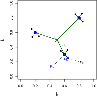
Figure 1: Schematic visualization of the hierarchical prior for a mixture of LCA models with three clusters, each containing three classes. For each cluster $k$, the occurrence probabilities $\bm{\pi}_{kl}=(\pi_{kl,j_{1}},\pi_{kl,j_{2}})$ of any two variables $j_{1}$ and $j_{2}$ in class $l$ (plotted as black points) are shrunken towards the cluster-centers $\bm{\mu}_{k}=(\mu_{k,j_{1}},\mu_{k,j_{2}})$ (plotted as large blue points) which in turn are shrunken towards the point $(1/D_{j},1/D_{j})=(0.5,0.5)$ (marked as a star).

2.2.3 Tuning the hyperparameters of the cluster distributions

The hierarchical prior on the occurrence probabilities $\bm{\pi}_{kl,j}$ needs to shrink (1) the marginal distribution of $\bm{\pi}_{kl,j}$ given $\bm{\mu}_{k,j}$ and the hyperparameters $(a_{\phi},c_{\phi},d_{\phi})$ towards the cluster-specific distribution $\bm{\mu}_{k,j}$ and (2) the cluster-specific distribution $\bm{\mu}_{k,j}$ towards a central distribution given the hyperparameter $a_{\mu}$. This requires careful selection of the hyperparameters $(a_{\phi},c_{\phi},d_{\phi})$ of the inverse gamma and gamma prior as well as the Dirichlet hyperparameter $a_{\mu}$ in the prior for $\bm{\mu}_{k,j}$ which are instrumental for learning the subcomponent occurrence probabilities $\bm{\pi}_{KL}$ jointly with the parameters $\bm{\mu}_{K}=(\bm{\mu}_{k,j})_{j=1,\ldots,r;k=1,\ldots,K}$ and $\bm{\phi}_{K}=(\phi_{k,j})_{j=1,\ldots,r;k=1,\ldots,K}$ from the data.

Specifying a supposedly uninformative prior for $\bm{\pi}_{kl,j}$ with $a_{\phi}=c_{\phi}=d_{\phi}=1$ leads to a diffuse marginal prior distribution $p(\bm{\pi}_{kl,j}|\bm{\mu}_{k,j},a_{\phi},c_{\phi},d_{\phi})$ which supports not only probabilities around the cluster-specific distribution $\bm{\mu}_{k,j}$, but also extreme probabilities close to 0 and 1. This can be seen in Figure 2 on the left-hand side, where the marginal prior distribution $p(\pi_{kl,j}|\mu_{k,j},a_{\phi},c_{\phi},d_{\phi})$ of the success probability $\pi_{kl,j}$ of category 1 for binary data with $D_{j}=2$ is plotted for $a_{\mu}=0.5$ (obtained using simulation). However, these extreme probability values close to 0 and 1 need to be avoided as they do not support the modeling aim of pulling the classes together by shrinking the occurrence probabilities towards the common component mean. In contrast, setting $c_{\phi}\gg 1$ leads to the desired shrinkage shape of the marginal occurrence probabilities, see Figure 2 in the middle and on the right-hand side.

Note that specifying a standard Dirichlet prior $\bm{\pi}_{kl,j}\sim\mathcal{D}_{D_{j}}(\bm{\alpha})$ with a fixed hyperparameter vector $\bm{\alpha}_{k,j}=\bm{\alpha}$ on the occurrence probabilities $\bm{\pi}_{kl,j}$ would also favor probabilities around a pre-specified mean value, if the sum over the elements in $\bm{\alpha}$ is large. However, compared to the marginal distribution obtained by decomposing the hyperparameter $\bm{\alpha}_{k,j}$ and specifying a hierarchical prior, less shrinkage towards the mean would be induced because of the platicurtic shape of the Dirichlet distribution, see Figure 2 in the middle and on the right-hand side, where the density of a beta distribution having the same mean and variance as the proposed marginal distribution is plotted with a solid black line.

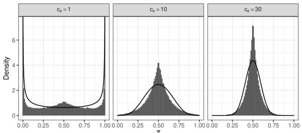
Figure 2: Marginal prior distribution $p(\pi_{kl,j}|\mu_{k,j},a_{\phi},c_{\phi},d_{\phi})$ of the success probability $\pi_{kl,j}$ of category 1 for a binary variable $j$ with $D_{j}=2$, assuming a beta distribution $\pi_{kl,j}\sim\mathcal{B}(\mu_{k,j}\phi_{j},(1-\mu_{k,j})\phi_{j})$ with $\mu_{k,j}=0.5$ for the success probability of category 1 in the cluster-specific average probability distribution $\bm{\mu}_{k,j}=(\mu_{k,j},1-\mu_{k,j})$, $\phi_{j}\sim\mathcal{G}^{-1}(a_{\phi},b_{\phi_{j}})$, and $b_{\phi_{j}}\sim\mathcal{G}(c_{\phi},d_{\phi})$ for $a_{\phi}=c_{\phi}=d_{\phi}=1$ (left), $a_{\phi}=1,c_{\phi}=10,d_{\phi}=1$ (middle) and $a_{\phi}=1,c_{\phi}=30,d_{\phi}=1$ (right). For comparison, the black line shows the beta distribution for $\pi_{kl,j}$ with the same mean and variance as the marginal prior distribution.

In the following we fix $a_{\phi}=d_{\phi}=1$ and only investigate in detail how different choices for $a_{\mu}$ and $c_{\phi}$ impact the results obtained. These hyperparameter values have a crucial influence on the amount of shrinkage and provide sufficient flexibility, even if $a_{\phi}$ and $d_{\phi}$ are fixed at 1.

3 Posterior inference

3.1 MCMC estimation

Bayesian estimation of the mixture of LCA models is performed using Markov chain Monte Carlo (MCMC) sampling with data augmentation. First, we consider the number of components $K$ a latent variable which is sampled during MCMC. Given $K$, the component and subcomponent assignments on the upper and lower level, $\mathbf{S}=(S_{1},\ldots,S_{N})$ and $\mathbf{I}=(I_{1},\ldots,I_{N})$, respectively, are added as latent variables and also drawn during MCMC sampling. Specifically, $S_{i}\in\{1,\ldots,K\}$ assigns each observation $\mathbf{y}_{i}$ to cluster $S_{i}$ on the upper level of the mixture of LCA models. On the lower level, $I_{i}\in\{1,\ldots,L\}$ assigns observation $\mathbf{y}_{i}$ to subcomponent $I_{i}$. Hence, the pair $(S_{i},I_{i})$ carries all the information needed to assign each observation to a unique class in the two-layer mixture.

In each iteration of the MCMC sampling scheme, the latent component assignments $(S_{1},\ldots,S_{N})$ on the upper level induce a random partition of the data, i.e., two observations $\mathbf{y}_{i}$ and $\mathbf{y}_{j}$ belong to the same cluster if and only if $S_{i}=S_{j}$. Thus the sampling scheme directly provides the posterior distribution of the partitions $\mathcal{C}=\{C_{1},\ldots,C_{K_{+}}\}$, with $C_{k}=\{i:S_{i}=k\}$ being the index set of observations assigned to cluster $k$, and $K_{+}$ the induced number of data clusters.

In order to obtain samples of $K$, and, conditional on $K$, of $(\mathbf{S},\bm{\eta}_{K},\bm{w}_{KL},\bm{\mu}_{K},\bm{\phi}_{K},\mathbf{I},\bm{\pi}_{KL},\alpha,\bm{b}_{\phi})$ from the posterior distribution, given data $\bm{y}=(\bm{y}_{1},\ldots,\bm{y}_{N})$, a transdimensional sampler is required which is able to sample parameter vectors of varying dimension. We use the telescoping sampler proposed by Frühwirth-Schnatter et al. (2021). This MCMC sampling scheme includes a sampling step where $K$ is explicitly sampled as an unknown parameter, but otherwise requires only sampling steps of a finite mixture model with a fixed number of components.

In particular, the telescoping sampler distinguishes explicitly between $K$, the number of components in the mixture distribution, and $K_{+}$, the number of “filled” components, i.e., components to which observations are assigned and which actually correspond to data clusters. Updating of the number of data clusters $K_{+}$ is implicitly performed, based on the sampled partition. In contrast, the number of components $K$ is explicitly sampled from the conditional posterior of $K$, given the current partition $\mathcal{C}$ which is characterized by the number of clusters $K_{+}$ and the number of observations $N_{k}=\#\{i|S_{i}=k\}$ assigned to each cluster $k=1,\ldots,K_{+}$. Using a dynamic specification for the Dirichlet prior on the weights, this posterior is proportional to the conditional partition distribution times the prior on $K$, i.e.,

$$p(K|\mathcal{C},\alpha) \propto p(\mathcal{C}|\alpha,K)p(K)$$ (3)

$$\propto\frac{K!}{(K-K_{+})!}\frac{\Gamma(\alpha)}{\Gamma(\alpha+N)}\prod_{k=1}^{K_{+}}\frac{\Gamma(N_{k}+\alpha/K)}{\Gamma(1+\alpha/K)}p(K),$$

where $\alpha$ is the hyperparameter of the symmetric Dirichlet prior $\bm{\eta}_{K}|K,\alpha\sim\mathcal{D}_{K}(\alpha/K)$. Importantly, sampling $K$ only depends on the current partition $\mathcal{C}$, and is independent of the component parameters. This makes the sampling scheme a generic sampler for arbitrary component densities and particularly useful for mixtures with complex component densities. More details on the telescoping sampler can be found in Frühwirth-Schnatter et al. (2021).

Conditional on $K$, sampling of the other parameters is straightforward as one can directly build on the standard sampling scheme for a mixture with fixed $K$. Gibbs updates based on the Dirichlet distribution are possible for the component and subcomponent weights as well as for the subcomponent occurrence probabilities on the lower level. For the parameters on the cluster level, Metropolis-Hastings steps are required to draw $\bm{\mu}_{k,j}$ and $\phi_{k,j}$ using a Dirichlet proposal for $\bm{\mu}_{k,j}$ and a random walk proposal for the logarithm of $\phi_{k,j}$. Updates on $\alpha$ are also generated by a Metropolis-Hastings step with a log-normal random walk proposal. Parameters for newly created, empty components are sampled from the priors. Sampling of hyperparameters is only based on information from the filled components. The MCMC sampling scheme including the initialization strategy pursued is reported in detail in Appendix B.

Due to multimodality of the posterior and mixing issues, inference is in the following based on 10 parallel runs. For each run, 4,000 iterations are recorded after discarding the first 1,000 iterations as burn-in. A specific run for further posterior inference is determined in the following way: First, the number of clusters $K_{+}$ is estimated by taking the most frequent mode of the posterior $p(K_{+}|\bm{y})$ across the 10 parallel runs. Then, among the runs where the mode corresponds to the selected $K_{+}$, the run with the highest mixture likelihood, is selected and used for further posterior inference.

3.2 Resolving label switching to obtain a final clustering

The draws from the posterior distribution require post-processing to resolve the label switching issue on the upper level to estimate a final clustering of the data. Many useful techniques have been proposed to post-process the sampled partitions (see, e.g., Papastamoulis, 2016; Wade and Ghahramani, 2018; Dahl et al., 2022). However, we would like to not only obtain a posterior estimate of a partition of the data but also perform posterior inference for the cluster-specific distributions, i.e., obtain the posterior distribution of the component-specific parameters. We adapt the procedure considered in Malsiner-Walli et al. (2017) to identify the model on the upper level. The procedure consists of the following steps.

First, a model selection step is performed by estimating the number of data clusters using the mode $\hat{K}_{+}$ of the posterior $p(K_{+}|\bm{y})$, i.e., by selecting the most frequent number of filled components during MCMC sampling. Only draws corresponding to iterations with exactly $\hat{K}_{+}$ filled components are included in the further analysis. Then, for each iteration and filled component, a low-dimensional functional of the class-specific parameters is computed to characterize the components. We use the averaged class occurrence probabilities weighted by their class weights as functional, i.e., $\tilde{\bm{\pi}}_{k,j}=\sum_{l=1}^{L}w_{kl}\bm{\pi}_{kl,j}$. These functionals are stacked on top of each other for the different components and the rows in the resulting matrix are clustered into $\hat{K}_{+}$ clusters using $k$-means clustering.

Using a functional of the class-specific parameters eases capturing the clusters in the parameter space. This is illustrated in Figure 3. For one run of the simulation study in Section 4 with three classes ($L=3$) on the lower and three filled components ($K_{+}=3$) on the upper level, Figure 3 shows scatter plots of the sampled class occurrence probabilities $\bm{\pi}_{kl,j}$ for all three classes within cluster $k$ (left-hand side), the cluster locations $\bm{\mu}_{k}$ (middle) and the functional $\tilde{\bm{\pi}}_{k,j}$ (right-hand side) for all three clusters $k=1,2,3$. Figure 3 on the left indicates that the class occurrence probabilities in the various clusters differ in their variability. In particular the rather diffuse subcomponents show an overlap within as well as across clusters, i.e., model identification is difficult if based directly on the class occurrence probabilities $\bm{\pi}_{kl,j}$. By contrast, the sampled component locations $\bm{\mu}_{k,j}$ are shrunken towards the center and exhibit considerable overlap, making identification based on $\bm{\mu}_{k,j}$ difficult (Figure 3 in the middle). However, a clear separation can be seen for the values of the functional $\tilde{\bm{\pi}}_{k,j}$ induced by the averaged class occurrence probabilities (Figure 3 on the right). These functionals thus represent the most suitable parameters for identifying the three clusters which clearly is an easy task based on these quantities.

Now $k$-means clustering is employed to assign each functional of the same iteration to a different group, inducing a unique labeling of the functional values. This unique labeling is used to reorder the components for all considered iterations thus obtaining identified values for the cluster weights $\bm{\eta}_{k}$, the cluster locations $\bm{\mu}_{k,j}$ and the cluster allocations $S_{i}$. A final partition of the data is obtained based on the maximum a posteriori (MAP) estimates of the relabeled component allocations $S_{i}$.

Note that on the lower level, in contrast to the upper level, identification of the classes is not required, as the LCA model is only intended to provide a semi-parametric approximation of the cluster distribution by capturing a possible association structure within the cluster. Thus, label switching among classes of the same component does not impact on the identification of the cluster distribution on the upper level and can be ignored, since the functional $\tilde{\bm{\pi}}_{k,j}$ is invariant to label switching among the $L$ classes in any cluster $k$.

Figure 3: Simulation study, $\rho=0.3$. Diagnostic plot of one MCMC run of a simulated data set with $L=3$, $a_{\mu}=20$, $c_{\phi}=30$, 1,000 iterations (after a burn-in of 1,000 iterations). For two variables ($j\in\{10,11\}$), scatter plots of the sampled $\bm{\pi}_{kl,j}$ (left), $\bm{\mu}_{k,j}$ (middle) and the cluster-specific functional $\tilde{\bm{\pi}}_{k,j}=\sum_{l=1}^{L}w_{kl}\bm{\pi}_{kl,j}$ (right) are shown.

4 Empirical demonstrations

4.1 Simulation study

The main focus of the simulation study is (1) to investigate whether the proposed Bayesian mixture of LCA models approach is able to estimate the true number of data clusters and the true partition of the data when the variables are associated within the clusters and (2) to contrast the performance to standard approaches for clustering multivariate categorical data based on the conditional independence assumption within clusters. We also investigate the influence of the specified number of subcomponents $L$ on the clustering results and perform a sensitivity analysis of the impact of the specified amount of shrinkage imposed by the chosen hyperparameters of the hierarchical prior on the occurrence probabilities.

Table 1: Simulation study. Occurrence probabilities $\mbox{\rm Pr}\{Y_{ij}=1|S_{i}=k\}$ for clusters $k=1,2,3$ and variables $j=1,\ldots,30$.

	V1	$\ldots$	V10	V11	$\ldots$	V20	V21	$\ldots$	V30
cluster 1	0.8	$\ldots$	0.8	0.8	$\ldots$	0.8	0.2	$\ldots$	0.2
cluster 2	0.2	$\ldots$	0.2	0.8	$\ldots$	0.8	0.2	$\ldots$	0.2
cluster 3	0.2	$\ldots$	0.2	0.2	$\ldots$	0.2	0.8	$\ldots$	0.8

Inspired by the low back pain data set (see Section 4.2), we define a mixture with three clusters of multivariate distributions on 30 binary variables as data generating mechanism. We consider two different scenarios regarding the within-cluster association between variables, one with associated variables and one where variables are independent. For both scenarios, the same marginal cluster-specific occurrence probabilities are assumed, as given in Table 1. In the first scenario, the within-cluster associations are generated by sampling from a multivariate discrete distribution with a given correlation matrix. The defined correlation matrix contains blocks of variables where within blocks all variables are pairwise correlated with correlation $\rho=0.3$. Outside the blocks the variables are independent. The three clusters differ in regard to location and size of the blocks in the correlation matrix. In cluster 1 and 2 only one block is present which consists of the first 15 and the middle 10 variables, respectively. Cluster 3 contains six blocks of successive variables. The association structure of this setup is visualized in Figure 4 in the bottom row, where for one data set the matrices containing the log-odds ratios of the success probabilities of the variables for each cluster and also for the whole data set are shown. The blocks of associated variables can be clearly identified through very high/low log-odds ratios.

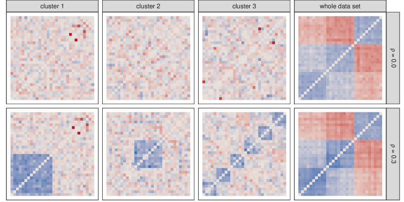
Figure 4: Simulation study. Top row: $\rho=0.0$; bottom row: $\rho=0.3$. Empirical results for one data set with $N=500$ of the log-odds ratios of the variables, conditional on cluster 1, 2 and 3 respectively and marginally across the whole data set (from left to the right).

The R (R Core Team, 2024) package GenOrd (Barbiero and Ferrari, 2015) is used to generate 30 data sets with 500 observations. The three clusters are specified to have the same group size. Package GenOrd employs a copula-based procedure for generating samples from discrete random variables with a prescribed correlation matrix and marginal distributions. Notably the association structure in the clusters are not generated by a LCA model. This means that the data generating process of the simulated data deviates from the modeling approach. Using this setting we show that the proposed approach is able to capture the association within a cluster, even if the cluster is not generated by a LCA model.

To each data set, a Bayesian mixture of LCA models is fitted with prior distributions and hyperparameters as described in Section 2.2. In particular, we use $K\sim\mathit{BNB}(1,4,3)$, $\alpha\sim\mathcal{G}(1,2)$, $\delta=1$, $a_{\phi}=d_{\phi}=1$. To investigate the impact of the hyperparameters $a_{\mu}$ and $c_{\phi}$ and the number of classes $L$ forming one cluster, a sensitivity analysis is performed. Specifically, the combination of the following values is investigated: $a_{\mu}\in(1,10,20,30)$, $c_{\phi}\in(1,10,20,30,40)$ and $L\in(2,3,4,5)$.

For each combination of prior parameter values, the specified model is fitted to each of the 30 data sets. As described in Section 3.1, for each data set, 10 parallel runs with 4,000 recorded iterations after discarding the first 1,000 iterations as burn-in are performed and, using the $K_{+}$ value estimated by the most frequent mode, the run with the highest mixture likelihood is used for further posterior inference. Convergence of the chains was assessed by visual inspection of the trace plots. Clustering performance is measured using the adjusted Rand index (ARI) which measures the classification agreement between the true and the estimated cluster memberships corrected for agreement by chance given the marginal cluster sizes. An ARI close to zero will be obtained for two independent partitions while an ARI close to 1 indicates perfect agreement between the two partitions.

Finally, we compare our results to the clustering results obtained by alternative methods. In particular, we use the package LCAvarsel (Fop, 2018) which combines LCA modeling with variable selection to omit redundant variables inducing association with the cluster distributions. In addition, we also perform standard latent class analysis based on maximum likelihood estimation with an expectation-maximization algorithm using the R packages BayesLCA (White and Murphy, 2014), Rmixmod (Lebret et al., 2015) and poLCA (Linzer and Lewis, 2011). Model selection is performed based on the Bayesian information criterion (BIC; BayesLCA, poLCA) and ICL (Rmixmod), after having fitted models with an increasing number of $K$ from 2 to 10 to all data sets and the packages are otherwise used with their default options. As an alternative Bayesian approach, we use package PReMiuM (Liverani et al., 2015) to fit an LCA model with a Dirichlet process prior. The number of initial clusters is set to 30, the number of burn-in draws and number of iterations are set to 2,000 and 10,000, respectively. All other settings, such as hyperparameter specifications, calculation of the similarity matrix and the derivation of the best partition, are left at the default values of the package. Additionally, PReMiuM with variable selection is performed using either the approach by Papathomas et al. (2012) (PReMiuM-contVS) or the method proposed by Chung and Dunson (2009) (PReMiuM-binVS).

Table 2 reports the clustering results obtained using the proposed Bayesian mixture of LCA models approach for each combination of prior hyperparameter values investigated. The average results obtained over the 30 data sets are reported. As expected, imposing a considerable amount of shrinkage supports the estimation of the true number of clusters $K^{\text{true}}=3$. In particular, specifying $a_{\mu}\geq 10$ and $c_{\phi}\geq 20$ leads to the estimation of three data clusters for almost all data sets. The specification of a larger number of classes $L$ also helps to obtain a sparser cluster solution. Results for $L=2$ indicate that two classes might not be sufficient to capture the association structure within the three clusters of the true data generating process and thus more than three clusters are frequently estimated, even if the prior parameter values induce a considerable amount of shrinkage. In case $L\geq 3$, results are comparable regardless of the specific value. This implies that $L=3$ seems to be sufficient to capture the association within the clusters in a suitable way and adding more classes does not improve but also does not lead to a deterioration of results. For hyperparameter values inducing a suitable amount of shrinkage as well as for $L\geq 3$, the average ARI is between 0.72 and 0.78. This value is clearly higher than the ARI of the clustering solutions obtained with the standard methods, see Table 3 on the left. Note that for the standard methods most of the time too many clusters are estimated (between four and eight), with the lowest number estimated for the variable selection approach proposed by Fop et al. (2017).

Overall, the clustering results of the Bayesian mixture of LCA models approach indicate that – at least for the investigated simulation scenario – the clustering results are robust in regard to moderate changes in the specification of the shrinkage parameters and the number of classes $L$, as long as they are chosen sufficiently large.

Figure 5 provides detailed insights into the specific MCMC results obtained for one run using $L=3$. On the top left, the trace plot of the sampled $K$ and the induced number of clusters $K_{+}$ is shown. Values considerably larger than three are sampled for $K$; the number of filled components $K_{+}$ switches between three and five, but are equal to $K_{+}=3$ most of the time. The barplots in Figure 5 in the middle indicate that both posterior distributions $p(K|\mathbf{y})$ and $p(K_{+}|\mathbf{y})$ have their mode at three. The trace plot on the top right hand side indicates convergence of the chain for the sampled $\alpha$ values. The trace plots at the bottom of Figure 5 show the number of observations allocated to the classes belonging to cluster 1, 2, and 3, respectively. In cluster 1 and 3 (first and third plot), the sizes of the three classes are quite distinct. In cluster 2 (second plot), there are two small classes where the number of observations assigned varies a lot. This suggests that perhaps at least one class is redundant. However, overfitting $L$ is allowed and does not have any impact on the cluster distribution. Scatter plots of the sampled class probabilities $\pi_{kl,j}$ have been shown in Figure 3.

Table 2: Simulation study. Clustering results (number of clusters $K_{+}$ and ARI) for various specifications of $a_{\mu}$, $c_{\phi}$, and $L$. $N=500$, $r=30$, correlation $\rho=0.3$. The true number of clusters is equal to 3, the number of simulated data sets is equal to 30.

		$K_{+}$					ARI
		$c_{\phi}$					$c_{\phi}$
	$a_{\mu}$	1	10	20	30	40	1	10	20	30	40
$L=2$	2	7.00	5.80	6.20	6.10	6.20	0.57	0.64	0.64	0.65	0.64
	10	7.00	4.50	3.60	3.40	3.40	0.54	0.67	0.75	0.76	0.77
	20	6.90	4.20	3.50	3.30	3.10	0.52	0.65	0.71	0.75	0.76
	30	7.20	4.20	3.60	3.40	3.30	0.51	0.62	0.69	0.73	0.74
$L=3$	2	5.90	5.20	5.40	5.60	5.90	0.62	0.65	0.67	0.65	0.64
	10	5.40	3.70	3.20	3.10	3.10	0.57	0.72	0.77	0.78	0.77
	20	5.60	3.80	3.30	3.10	3.10	0.54	0.67	0.73	0.75	0.76
	30	5.50	3.70	3.30	3.20	3.10	0.51	0.63	0.71	0.74	0.75
$L=4$	2	5.10	4.60	5.00	5.30	5.80	0.65	0.67	0.66	0.64	0.65
	10	4.60	3.30	3.10	3.00	3.10	0.62	0.75	0.78	0.78	0.77
	20	4.80	3.50	3.20	3.10	3.00	0.55	0.68	0.75	0.77	0.77
	30	5.00	3.40	3.30	3.20	3.10	0.53	0.66	0.72	0.74	0.75
$L=5$	2	4.70	4.60	4.90	5.20	5.40	0.68	0.71	0.70	0.66	0.64
	10	4.20	3.10	3.00	3.10	2.90	0.62	0.76	0.78	0.77	0.75
	20	4.20	3.30	3.10	3.00	3.00	0.55	0.72	0.76	0.77	0.77
	30	4.40	3.40	3.20	3.20	3.10	0.53	0.68	0.73	0.74	0.75

Table 3: Simulation study. Clustering results (number of clusters $K_{+}$, ARI and err) for alternative methods. $N=500$, $r=30$, correlation $\rho=0.3$ (left) and $\rho=0.0$ (right). The true number of clusters is equal to 3, the number of simulated data sets is equal to 30.

	$\rho=0.3$			$\rho=0.0$
	$K_{+}$	ARI	err	$K_{+}$	ARI	err
LCAvarsel	3.43	0.67	0.15	3.00	0.96	0.02
BayesLCA	4.07	0.68	0.21	3.00	0.96	0.02
PoLCA	4.17	0.67	0.21	3.03	0.95	0.02
Rmixmod	7.07	0.68	0.19	3.20	0.95	0.02
PReMiuM	8.67	0.52	0.36	3.13	0.96	0.02
PReMiuM-contVS	7.93	0.56	0.31	3.07	0.95	0.02
PReMiuM-binVS	8.23	0.54	0.34	3.17	0.95	0.02

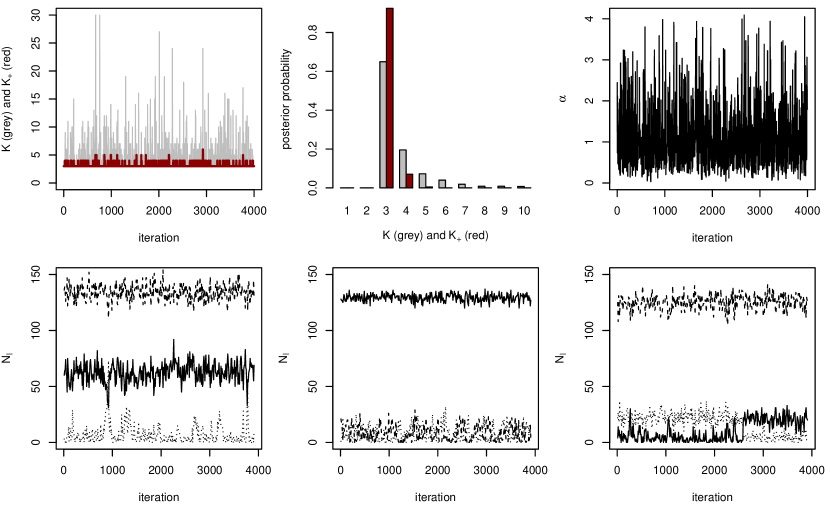
Figure 5: Simulation study, $\rho=0.3$. Diagnostic plot of one MCMC run of a simulated data set with $L=3$, $a_{\mu}=20$, $c_{\phi}=30$, 4,000 iterations (after a burn-in of 1,000 iterations). Top: trace plot (left) and posterior distribution (middle) of the number of components $K$ (gray) and number of data clusters $K_{+}$ (red), sampled hyperparameter $\alpha$ (right). Bottom: trace plot of the number of observations assigned to subcomponent $l=1,2,3$ for cluster 1, 2 and 3 (from left to right).

The aim of the second simulation scenario is to investigate how the specified Bayesian mixture of LCA models performs if variables within clusters are independent, i.e., if the standard conditional independence assumption of the LCA model applies to the cluster distributions. The data generating process is basically the same as for the first scenario, the only difference is that the pairwise correlation in blocks is set to $\rho=0.0$. The matrices showing the pairwise log-odds within clusters and for the whole data set are provided in Figure 4 in the top row.

Table 4 reports the clustering results of the proposed Bayesian mixture of LCA models approach for each combination of prior parameter values investigated. In the case of independent clusters, the Bayesian modeling approach consistently estimates three clusters with an ARI around 0.95 for all prior specifications which also performed well in the simulations scenario with correlated clusters. These results also coincide with the favorable results obtained with the standard methods, as shown in Table 3 on the right. The good performance of the Bayesian mixture of LCA models approach also in the case where its flexibility is indeed not required implies that it can be employed even if the user is unsure about the dependency structure within the clusters they are aiming for.

Table 4: Simulation study. Clustering results (number of clusters $K_{+}$ and ARI) for various specifications of $a_{\mu}$, $c_{\phi}$, and $L$. $N=500$, $r=30$, correlation $\rho=0.0$. The true number of clusters is equal to 3, the number of simulated data sets is equal to 30.

		$K_{+}$					ARI
		$c_{\phi}$					$c_{\phi}$
	$a_{\mu}$	1	10	20	30	40	1	10	20	30	40
$L=2$	2	3.00	3.00	3.00	2.90	2.80	0.96	0.95	0.95	0.92	0.87
	10	3.00	3.00	3.00	3.00	3.00	0.95	0.96	0.96	0.96	0.95
	20	3.00	3.00	3.00	3.00	3.00	0.95	0.95	0.95	0.96	0.95
	30	3.00	3.00	3.00	3.00	3.00	0.95	0.95	0.95	0.95	0.95
$L=3$	2	3.00	3.00	2.90	2.70	2.60	0.95	0.94	0.89	0.84	0.80
	10	3.00	3.00	3.00	3.00	3.00	0.95	0.95	0.96	0.95	0.95
	20	3.00	3.00	3.00	3.00	3.00	0.95	0.95	0.96	0.96	0.96
	30	3.00	3.00	3.00	3.00	3.00	0.96	0.96	0.95	0.95	0.95
$L=4$	2	3.00	3.00	2.80	2.70	2.50	0.95	0.93	0.85	0.82	0.76
	10	3.00	3.00	3.00	3.00	3.00	0.95	0.95	0.96	0.95	0.95
	20	3.00	3.00	3.00	3.00	3.00	0.95	0.95	0.96	0.96	0.95
	30	3.00	3.00	3.00	3.00	3.00	0.95	0.96	0.96	0.95	0.95
$L=5$	2	3.00	2.90	2.70	2.70	2.70	0.95	0.92	0.81	0.81	0.81
	10	3.00	3.00	3.00	3.00	3.00	0.95	0.96	0.95	0.95	0.95
	20	3.00	3.00	3.00	3.00	3.00	0.95	0.96	0.96	0.95	0.96
	30	3.00	3.00	3.00	3.00	3.00	0.95	0.96	0.96	0.96	0.95

4.2 Low back pain data

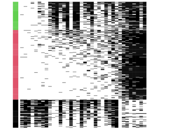
Figure 6: Low back pain data. Visualization of the original data matrix with patients in the rows and the binary variables in the columns. Patients are ordered by the expert-based grouping with the grouping indicated by color on the left and within-grouping by the average agreement level; columns are also ordered by the average agreement level.

Fop et al. (2017) use model-based clustering to analyze a multivariate binary data set on low back pain for 425 patients on 36 questions about the presence or absence of certain pain symptoms. An expert-based classification of the patients into three groups is available which serves as a gold standard. Figure 6 provides a visualization of the binary data matrix, with the rows ordered by the expert-based grouping and within the grouping by average agreement level and columns ordered by average agreement level.

Table 5: Low back pain data. Clustering results (number of clusters $K_{+}$ and ARI) for various specifications of $a_{\mu}$, $c_{\phi}$, and $L$.

		$K_{+}$					ARI
		$c_{\phi}$					$c_{\phi}$
	$a_{\mu}$	1	10	20	30	40	1	10	20	30	40
$L=2$	2	11.00	6.00	5.00	5.00	4.00	0.37	0.46	0.49	0.65	0.80
	10	9.00	5.00	4.00	3.00	3.00	0.38	0.45	0.68	0.82	0.80
	20	9.00	5.00	4.00	3.00	3.00	0.37	0.53	0.68	0.80	0.79
	30	9.00	5.00	3.00	3.00	3.00	0.39	0.43	0.82	0.79	0.80
$L=3$	2	8.00	5.00	4.00	4.00	4.00	0.45	0.49	0.79	0.79	0.80
	10	8.00	3.00	3.00	3.00	3.00	0.36	0.74	0.81	0.81	0.82
	20	9.00	5.00	3.00	3.00	3.00	0.53	0.40	0.81	0.72	0.80
	30	8.00	4.00	3.00	3.00	3.00	0.34	0.59	0.81	0.73	0.79
$L=4$	2	8.00	5.00	4.00	5.00	4.00	0.43	0.51	0.75	0.53	0.80
	10	7.00	4.00	3.00	3.00	3.00	0.33	0.68	0.69	0.83	0.83
	20	8.00	4.00	3.00	3.00	3.00	0.34	0.50	0.81	0.74	0.79
	30	8.00	4.00	3.00	3.00	3.00	0.35	0.49	0.72	0.73	0.79
$L=5$	2	7.00	5.00	5.00	4.00	4.00	0.46	0.43	0.49	0.80	0.80
	10	6.00	4.00	3.00	3.00	3.00	0.40	0.45	0.71	0.82	0.83
	20	7.00	4.00	3.00	3.00	3.00	0.39	0.47	0.83	0.80	0.80
	30	7.00	4.00	3.00	3.00	3.00	0.41	0.69	0.83	0.75	0.81

For this data set, the presence of within-cluster correlation is indicated by the following results. On the one hand, a standard LCA model fitted to this data set including all variables overestimates the number of clusters in the data, e.g., estimating the LCA model with maximum likelihood using the R package poLCA results in five components. On the other hand, fitting a standard LCA model to each expert-based class using maximum likelihood estimation, results in LCA models with two components for expert-based class 1 or 2, and one component for expert-based class 3.

Fop et al. (2017) pursue a variable selection approach to obtain an LCA model where classes correspond to the grouping induced by the expert-based classification (see Table 6). Using the Bayesian mixture of LCA models approach, we also aim at identifying the expert-based grouping but without eliminating redundant variables which induce within-cluster correlation.

The clustering results of the Bayesian mixture of LCA models approach are reported in Table 5 for varying number of subcomponents $L$ and prior parameters $a_{\mu}$ and $c_{\phi}$. For each parameter combination, ten runs of the MCMC sampling scheme are performed and results are reported for the run selected using the procedure described in Section 4.1. The results are in line with those obtained for the simulation study with correlated clusters. Specifying shrinkage priors with $c_{\phi}\geq 20$, $a_{\mu}\geq 10$ and $L\geq 3$, results in a good clustering performance with three clusters being estimated. The ARI is at least 0.69 and the largest value obtained is 0.83. The largest value achieved outperforms even the value of 0.79 reported by Fop et al. (2017). The alternative methods proposed for clustering multivariate categorical data – except for the variable selection approach proposed by Fop et al. (2017) – estimate between 5 and 10 clusters with an ARI around 0.50, see Table 6. Thus, the Bayesian mixture of LCA models using priors inducing considerable amount of shrinkage succeeds in capturing the associated clusters in the back pain data set, avoiding the appearance of spurious clusters, which are included when fitting a standard LCA model due to the independence assumption.

Table 6: Low back pain data. Alternative methods, with their default settings, 10 runs.

	$K_{+}$	ARI	err
LCAvarsel	3	0.73	0.09
BayesLCA	5	0.50	0.39
PoLCA	5	0.48	0.39
Rmixmod	5	0.50	0.38
PReMiuM	8	0.40	0.47
PReMiuM-contVS	8	0.42	0.46
PReMiuM-binVS	9	0.42	0.43

5 Summary

In the Bayesian framework of model-based clustering of multivariate categorical data, this paper addresses the issue of dealing with associated variables within a cluster. We propose to model each cluster by a LCA model capturing possible within-cluster associations. The resulting two-layer mixture of LCA models is completed through the specification of carefully selected shrinkage priors. The use of shrinkage priors supports the modeling aims in model-based clustering, i.e., they enable the identification of the two-layer model and the automatic estimation of a sparse number of clusters. Note that the proposed approach relies crucially on the specification of shrinkage priors. However, the defined shrinkage priors serve different purposes and can be thought of as a kind of regularization or soft constraint imposed on the different levels in the model estimation.

Specifically, on the lower level shrinkage of the class occurrence probabilities forming one cluster towards the cluster center probabilities allows identification of the cluster distributions. The likelihood of a two-layer mixture model is invariant to changing the assignment of subcomponents to components. Shrinkage priors ensure that subcomponents are pulled towards a common cluster centroid, in this way inducing identifiability and destroying the invariance. On the upper level, shrinking the centers of the cluster distributions toward the uniform distribution supports the estimation of a small number of clusters, as the cluster distributions are enforced to be more similar. This shrinkage also acts as a kind of variable selection procedure; the occurrence probabilities of a single variable are thereby pulled towards the uniform distribution, reducing their contribution to the likelihood and suppressing in this way the appearance of additional noisy clusters.

Finally, controlling against overfitting the number of components $K$ is achieved by specifying appropriate priors on $K$ and the mixture weights which a priori will induce a large weight on partitions with a small number of clusters. The shrinkage prior for $K$ favors the homogeneity model and only allows a deviation from the one-cluster model if the heterogeneity in the data is strong enough. Additionally, the shrinkage prior on the mixture weights on the upper level obtained through the dynamic specification prevents that the number of clusters increases as fast as the number of proposed components.

The telescoping sampler, where sampling the number of components $K$ is conditionally independent of the component-specific parameters, has clear advantages when fitting a mixture distribution with complex component densities to data with an unknown number of clusters. The mixture of LCA models is a nice example for the application of the telescoping sampler as for this model it might be too cumbersome to design acceptable proposals for employing RJMCMC or integrate out the parameters for sampling the indicators marginally as required for the samplers used in Bayesian non-parametric mixture analysis.

Extensions of the proposed approach could be considered in several directions. The clustering of multivariate categorical data often involves many variables. Co-clustering (Govaert and Nadif, 2013), also known as biclustering or two-mode clustering, aims at simultaneously grouping rows and columns of a rectangular data matrix. Simultaneously clustering rows and columns of a multivariate categorical data matrix eases interpretation by providing a natural grouping of variables. It would thus be of interest to extend the proposed Bayesian mixture of LCA models approach with a prior on the number of components to also cluster the columns. Alternatively one could also investigate a Bayesian two-layer mixture model for modeling multivariate count data, e.g., using mixtures of independent Poisson distributions on the lower level.

Appendix A The beta-negative-binomial distribution

The beta-negative-binomial (BNB) distribution is a three-parameter distribution with support on the non-negative integers. The distribution results as a hierarchical generalization of the Poisson, the geometric and the negative-binomial distribution.

A translated version is considered for the number of components $K$ with the probability mass function corresponding to $K-1\sim\mathit{BNB}(r,\alpha,\beta)$ given by:

$$p(K) =\frac{\Gamma(r+K-1)\text{B}(r+\alpha,K-1+\beta)}{\Gamma(r)\Gamma(K)\text{B}(\alpha,\beta)}.$$ (4)

The mean of $K$ exists for $\alpha>1$ and is equal to $1+r\frac{\beta}{\alpha-1}$. The different shapes of the BNB distribution obtained for various values of the parameters are illustrated in Figure 7.

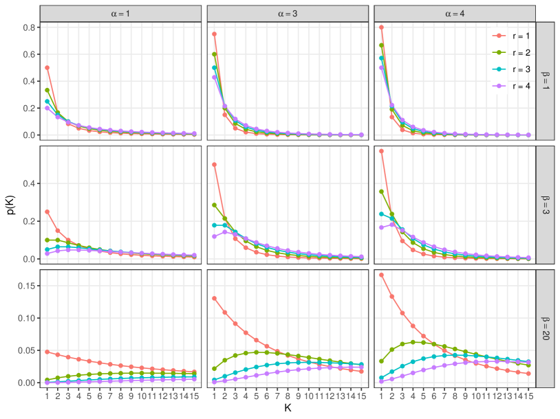
Figure 7: Priors $p(K)$ derived from the translated prior $K-1\sim\mathit{BNB}(r,\alpha,\beta)$ for various parameter values.

Appendix B MCMC sampling scheme

Posterior inference for the Bayesian mixture of LCA models is performed through MCMC sampling based on data augmentation and Gibbs sampling. First, the number of components $K$ is considered a latent variable. Second, to indicate the component to which each observation belongs, latent allocation variables $\mathbf{S}=(S_{1},\ldots,S_{N})$ taking values in $\{1,\ldots,K\}$ are introduced such that

$$p(\mathbf{y}_{i}|\bm{\theta}_{1},\ldots,\bm{\theta}_{K},S_{i}=k) =p_{k}(\mathbf{y}_{i}|\bm{\theta}_{k}).$$

Additionally, latent allocation variables $\mathbf{I}=(I_{1},\ldots,I_{N})$ taking values in $\{1,\ldots,L\}$ are introduced to indicate the subcomponent to which an observation within a component is assigned. This implies

$$p(\mathbf{y}_{i}|S_{i}=k,\bm{\theta}_{k},I_{i}=l) =\prod_{j=1}^{r}\prod_{d=1}^{D_{j}}\pi_{kl,jd}^{I\{y_{ij}=d\}}.$$

The latent variables $(\mathbf{S},\mathbf{I})$ and parameters $(K,\bm{\eta}_{K},\alpha,\bm{w}_{KL},\bm{\pi}_{KL},\bm{\phi}_{K},\bm{\mu}_{K},\bm{b}_{\phi})$ are sampled using the following Gibbs sampling scheme after suitable initialization.

The MCMC scheme is initialized by assigning observations to a component as well as to subcomponents within a component, i.e., by specifying the latent variables $(\mathbf{S},\mathbf{I})$. The assignment vector $\mathbf{S}$ is determined using $k$-means clustering starting with an overfitting number of clusters (e.g., $K=10$ in the empirical demonstrations). Within each component, the subcomponent assignment vector $\mathbf{I}$ is then obtained using random assignment with equal probabilities to initially obtain comparable subcomponent distributions within a component. Based on the classification induced by $(\mathbf{S},\mathbf{I})$, the initial occurrence probabilities are obtained as the empirical occurrence probabilities within each of the subcomponents. The initial values for $\bm{\mu}_{k,j}$ and $\phi_{k,j}$ are set to the vector of length $D_{j}$ with identical values $1/D_{j}$ and $D_{j}$, respectively.

The MCMC sampling scheme then proceeds as follows:

1. For a given $K$, update the partition of the data:

   1. Sample $S_{i}$ for $i=1,\ldots,N$ from $p(S_{i}|K,\bm{\eta}_{K},\bm{\theta}_{1},\ldots,\bm{\theta}_{K},{\mathbf{y}})$, marginalized w.r.t. the subcomponent indicator $\mathbf{I}$, using:

      $$\mbox{\rm Pr}\{S_{i}=k|K,{\bm{\eta}}_{K},\bm{\theta}_{1},\ldots,\bm{\theta}_{K},{\mathbf{y}}_{i}\}\propto\eta_{k}p_{k}({\mathbf{y}}_{i}|\bm{\theta}_{k}),\quad k=1,\ldots,K,$$

      where $p_{k}(\mathbf{y}_{i}|\bm{\theta}_{k})$ is the cluster density given by a LCA model:

      $$p_{k}(\mathbf{y}_{i}|\bm{\theta}_{k})=\sum_{l=1}^{L}w_{kl}\prod_{j=1}^{r}\prod_{d=1}^{D_{j}}\pi_{kl,jd}^{I\{y_{ij}=d\}}.$$

   2. Determine $K_{+}=\sum_{k=1}^{K}I\{N_{k}>0\}$, where $N_{k}=\#\{i|S_{i}=k\}$.

   3. Relabel the components such that the first $K_{+}$ components are non-empty.

2. Conditional on $\mathbf{S}$, update the parameters and hyperparameters for each filled cluster $k=1,\ldots,K_{+}$:

   1. Sample subcomponent indicators from

      $$\mbox{\rm Pr}\{I_{i}=l|S_{i}=k,\mathbf{y}_{i},\cdot\} \propto w_{kl}\prod_{j=1}^{r}\prod_{d=1}^{D_{j}}\pi_{kl,jd}^{I\{y_{ij}=d\}},\quad l=1,\ldots,L.$$

   2. Sample subcomponent weights from

      $$\bm{w}_{k}|\mathbf{I},\mathbf{S}\sim\mathcal{D}_{L}(d_{k1},\ldots,d_{kL}),\quad l=1,\ldots,L,$$

      using $d_{kl}=\delta+N_{kl}$ where $N_{kl}=\#\{i|I_{i}=l,S_{i}=k\}$ is the number of observations allocated to subcomponent $l$ in cluster $k$.

   3. Sample subcomponent occurrence probabilities from

      $$\bm{\pi}_{kl,j}|\bm{\mu}_{k,j},\phi_{k,j},\mathbf{S},\mathbf{y}\sim\mathcal{D}_{D_{j}}(\mathbf{a}_{kl,j}),$$

      where

      $$\mathbf{a}_{kl,j} =\bm{\mu}_{k,j}\phi_{k,j}+a_{00}\bm{1}_{D_{j}}+\bm{N}_{kl,j},$$

      with $\bm{N}_{kl,j}=(N_{kl,j1},\ldots,N_{kl,jD_{j}})$ and where $N_{kl,jd}$ indicates how often in subcomponent $l$ of cluster $k$ category $d$ is observed for feature $j$:

      $$N_{kl,jd} =\sum_{\iota\in\{i|S_{i}=k,I_{i}=l\}}I\{y_{\iota j}=d\}.$$

   4. Sample hyperparameters for $j=1,\ldots,r$:

      • Sample $\bm{\mu}_{k,j}$ from $p(\bm{\mu}_{k,j}|a_{\mu})\cdot\prod_{l=1}^{L}p(\bm{\pi}_{kl,j}|\bm{\mu}_{k,j},\phi_{k,j},a_{00})$, i.e.,

        $$\propto\mu_{k,j1}^{a_{\mu}-1}\cdots\mu_{k,jD_{j}}^{a_{\mu}-1}\prod_{l=1}^{L}\mathcal{D}_{D_{j}}(\bm{\pi}_{kl,j}|\bm{\mu}_{k,j}\phi_{k,j}+a_{00}\bm{1}_{D_{j}})$$

        using a Metropolis-Hastings step with Dirichlet proposal density

        $$\bm{\mu}_{k,j}^{new}\sim\mathcal{D}_{D_{j}}(\bm{\mu}_{k,j}^{old}s_{\mu}),$$

        where $s_{\mu}$ is a fixed precision value acting as a calibration parameter.

      • Sample $\phi_{k,j}$ from $p(\phi_{k,j}|a_{\phi},b_{\phi_{j}})\cdot\prod_{l=1}^{L}p(\bm{\pi}_{kl,j}|\bm{\mu}_{k,j},\phi_{k,j},a_{00})$,
        i.e.

        $$\propto\phi_{k,j}^{-a_{\phi}-1}\exp(-b_{\phi_{j}}/\phi_{k,j})\cdot\prod_{l=1}^{L}\mathcal{D}_{D_{j}}(\bm{\pi}_{kl,j}|\bm{\mu}_{k,j}\phi_{k,j}+a_{00}\bm{1}_{D_{j}})$$

        using a random walk Metropolis-Hastings step with proposal

        $$\log(\phi_{k,j}^{new})\sim\mathcal{N}(\log(\phi_{k,j}^{old}),s^{2}_{\phi}),$$

        where $s^{2}_{\phi}$ is a fixed variance value acting as a calibration parameter.

3. Sample the dimension-specific hyperparameter for the precision of the component location for $j=1,\ldots,r$:

   • Sample $b_{\phi_{j}}$ from

     $$b_{\phi_{j}} \sim\mathcal{G}(c_{\phi_{j}},d_{\phi_{j}}),$$

     where

     $$c_{\phi_{j}} =c_{\phi}+K_{+}a_{\phi}, d_{\phi_{j}} =d_{\phi}+\sum_{k=1}^{K_{+}}\frac{1}{\phi_{k,j}}.$$

4. Conditional on $\mathcal{C}$, sample $K$ and $\alpha$:

   1. Sample $K$ from

      $$p(K|\mathcal{C},\alpha) \propto p(K)\frac{\alpha^{K_{+}}K!}{K^{K_{+}}(K-K_{+})!}\prod_{k=1}^{K_{+}}\frac{\Gamma(N_{k}+\frac{\alpha}{K})}{\Gamma(1+\frac{\alpha}{K})},\quad K=K_{+},K_{+}+1,\ldots,K_{\max}.$$

      In theory, $K_{\max}$ is infinite. For the computational implementation, a finite value is pre-specified. A value large enough to capture all relevant values of $K$ needs to be selected, but as small as possible to reduce computational complexity.

   2. Use a random walk Metropolis-Hastings step with proposal $\log(\alpha^{new})\sim\mathcal{N}({\log(\alpha^{old}),s_{\alpha}^{2}})$ to sample $\alpha|\mathcal{C},K$ from

      $$p(\alpha|\mathcal{C},K) \propto p(\alpha)\frac{\alpha^{K_{+}}\Gamma(\alpha)}{\Gamma(N+\alpha)}\prod_{k=1}^{K_{+}}\frac{\Gamma(N_{k}+\frac{\alpha}{K})}{\Gamma(1+\frac{\alpha}{K})}.$$

5. Add $K-K_{+}$ empty components and update the component weight distribution conditional on $K,\mathcal{C},\alpha$ and $\phi$:

   1. If $K>K_{+}$, then add $K-K_{+}$ empty components (i.e., $N_{k}=0$ for $k=K_{+}+1,\ldots,K$) by sampling $\bm{w}_{k}$ from the symmetric Dirichlet prior for $k=K_{+}+1,\ldots,K$:

      $$\bm{w}_{k}|d_{0}\sim\mathcal{D}_{L}(\delta),$$

      and sampling $\bm{\theta}_{k}$ for $k=K_{+}+1,\ldots,K$ from the hierarchical prior defined for $\bm{\pi}_{kl,j}|b_{\phi_{j}},a_{\phi},a_{\mu},a_{00}$ for $j=1,\dots,r$, conditional on the current value of $b_{\phi_{j}}$:

      $$\bm{\mu}_{k,j}|a_{\mu} \sim\mathcal{D}_{D_{j}}(a_{\mu}),$$

      $$\phi_{k,j}|a_{\phi},b_{\phi_{j}} \sim\mathcal{G}^{-1}(a_{\phi},b_{\phi_{j}}),$$

      $$\bm{\pi}_{kl,j}|a_{00},\bm{\mu}_{k,j},\phi_{k,j} \sim\mathcal{D}_{D_{j}}(\bm{\mu}_{k,j}\phi_{k,j}+a_{00}\bm{1}_{D_{j}}),\quad l=1,\ldots,L.$$

   2. Sample

      $$\bm{\eta}_{K}|K,\alpha,\mathcal{C} \sim\mathcal{D}_{K}(\gamma_{1},\ldots,\gamma_{K}),$$

      where $\gamma_{k}=\alpha/K+N_{k}$.

3 References

References

- Agresti (2002) Agresti, A. (2002). Categorical Data Analysis (2nd ed.). Wiley Series in Probability and Statistics. New York, NY: John Wiley & Sons.
- Barbiero and Ferrari (2015) Barbiero, A. and P. A. Ferrari (2015). GenOrd: Simulation of Discrete Random Variables with Given Correlation Matrix and Marginal Distributions. R package version 1.4.0.
- Bartolucci et al. (2016) Bartolucci, F., G. E. Montanari, and S. Pandolfi (2016). Item selection by latent class-based methods: An application to nursing home evaluation. Advances in Data Analysis and Classification 10(2), 245–262.
- Bock (1986) Bock, H.-H. (1986). Loglinear models and entropy clustering methods for qualitative data. In W. Gaul and M. Schader (Eds.), Classification as a Tool of Research, pp. 19–26.
- Chung and Dunson (2009) Chung, Y. and D. B. Dunson (2009). Nonparametric Bayes conditional distribution modeling with variable selection. Journal of the American Statistical Association 104(488), 1646–1660.
- Dahl et al. (2022) Dahl, D. B., D. J. Johnson, and P. Müller (2022). Search algorithms and loss functions for bayesian clustering. Journal of Computational and Graphical Statistics 31(4), 1189–1201.
- Dean and Raftery (2010) Dean, N. and A. E. Raftery (2010). Latent class analysis variable selection. The Annals of the Institute of Statistical Mathematics 62(1), 11.
- Durante et al. (2017) Durante, D., D. B. Dunson, and J. T. Vogelstein (2017). Nonparametric Bayes modeling of populations of networks. Journal of the American Statistical Association 112(520), 1516–1530.
- Fop (2018) Fop, M. (2018). LCAvarsel: Variable Selection for Latent Class Analysis. R package version 1.1.
- Fop et al. (2017) Fop, M., K. M. Smart, and T. B. Murphy (2017). Variable selection for latent class analysis with application to low back pain diagnosis. The Annals of Applied Statistics 11(4), 2080–2110.
- Frühwirth-Schnatter (2006) Frühwirth-Schnatter, S. (2006). Finite Mixture and Markov Switching Models. New York: Springer-Verlag.