See Further for Parameter Efficient Fine-tuning by Standing on the Shoulders of Decomposition

Abstract

The rapid expansion of large foundation models within the pre-training and fine-tuning framework has underscored that larger models often yield better results. However, the scaling up of large foundation models has led to soaring costs in fine-tuning and parameter storage, rendering extensive adaptations impractical. This challenge has sparked the development of parameter-efficient fine-tuning (PEFT), which focuses on optimizing a select subset of parameters while keeping the rest fixed, significantly lowering computational and storage overheads. While recent years have witnessed a significant success in PEFT, a deep understanding of the fundamental principles behind these methods remains unexplored. To this end, here we take the first step to unify all approaches by dissecting them from a decomposition perspective. We initiate a comprehensive mathematical analysis of these methods, allowing us to delve deeply into their underlying mechanisms, and we explore the reasons behind the variations in performance among different techniques. Furthermore, inspired by our theoretical analysis, we introduce two novel PEFT methods alongside a simple yet effective framework designed to enhance the performance of PEFT techniques across various applications. Our empirical validations, conducted across multiple datasets, demonstrate the efficacy of these methods, showcasing both theoretical validity and practical performance improvements under the guidance of our analytical findings. Moreover, to support research in subspace tuning, we are developing an open-source toolkit called Subspace-Tuning. This toolkit allows practitioners to efficiently and flexibly implement subspace tuning on different pretrained models for different tasks. We believe our work will deepen researchers’ understanding of PEFT and other techniques, prompting further contemplation and advancing the research across the whole community.

Keywords —- parameter efficient, decomposition theory, subspace tuning

If I have seen further

it is by standing on the shoulders of giants.

– Isaac Newton

1 Introduction

The emergence of foundation models, as referenced in multiple studies (Brown et al. (2020); Radford et al. (2019, 2021); Devlin et al. (2018); Liu et al. (2019)), has fundamentally altered the landscape of artificial intelligence, demonstrating substantial effectiveness across a variety of domains. For example, Segment Anything Model (SAM) (Kirillov et al. (2023)) has been widely implemented across a variety of visual tasks (Zhang and Liu (2023); Si et al. (2024b); Zhang et al. (2023)), and Generative Pre-trained Transformer (GPT) (Brown et al. (2020); Radford et al. (2019)) has even seamlessly integrated into our daily lives, evolving into an exceedingly practical tool (Achiam et al. (2023); Waisberg et al. (2023); Mao et al. (2023)). Traditionally, the adaptation of pre-trained models to specific downstream tasks required fully fine-tuning of all parameters (Ma et al. (2024); Raffel et al. (2020); Qiu et al. (2020)). However, as the complexity and size of these models have increased, this traditional approach to fine-tuning has become less feasible, both from a computational and resource standpoint.

In response to these challenges, there has been a pivot towards developing more parameter-efficient fine-tuning techniques (Chen et al. (2024); Guo et al. (2020); He et al. (2021a); Hu et al. (2021)), collectively known as parameter-efficient fine-tuning (PEFT). The goal of PEFT is to achieve comparable performance on downstream tasks by tuning a minimal number of parameters. Presently, PEFT strategies can be categorized into three predominant groups (Liu et al. (2024); Ding et al. (2023)), each with its distinctive mechanisms and intended use cases.

Firstly, adapter-based methods, as discussed in several works (Houlsby et al. (2019); Chen et al. (2022); Luo et al. (2023); He et al. (2021a); Mahabadi et al. (2021); Karimi Mahabadi et al. (2021)), involve the insertion of small, trainable linear modules within the pre-existing network architectures. These modules are designed to adapt the model’s outputs without changing the original network weights. Secondly, the prompt-based approaches (Lester et al. (2021); Razdaibiedina et al. (2023); Wang et al. (2023); Shi and Lipani (2023); Fischer et al. (2024)) make use of mutable soft tokens placed at the beginning of inputs. This strategy focuses on fine-tuning these prompts to steer the model’s behavior during specific tasks. Thirdly, low-rank decomposition approaches like LoRA (Hu et al. (2021); Liu et al. (2024); Hyeon-Woo et al. (2021); Qiu et al. (2023); Renduchintala et al. (2023); Kopiczko et al. (2023); YEH et al. (2023); Zhang et al. (2022); Si et al. (2024c)) are applied to network weights during fine-tuning, enhancing their adaptability while maintaining overall compatibility with the pre-trained settings. Additionally, the landscape of PEFT is enriched by other innovative methods such as BitFit (Zaken et al. (2021); Lawton et al. (2023)), which focus solely on fine-tuning bias terms. Collectively, these diverse strategies significantly augment the adaptability and efficiency of models, enabling them to meet specific task requirements without the need for extensive retraining. Through these developments, the whole community continues to evolve towards more sustainable and manageable model training methodologies.

However, despite that recent years have witnessed significant advancements in PEFT (Han et al. (2024); He et al. (2021a); Fu et al. (2023)), the mathematical foundations underpinning different PEFT methods have scarcely been studied. Moreover, the performance differences between various PEFT methods and the reasons behind these differences have not been systematically explored. This lack of theoretical depth limits our understanding of the potential advantages and limitations of these methods, hindering their optimization and innovation in practical applications. Therefore, conducting theoretical research in this field will be crucial for advancing PEFT technologies, providing a fundamental basis for selecting and designing more efficient fine-tuning strategies.

Therefore, in this paper, we undertake a pioneering theoretical examination of PEFT techniques, leveraging insights from decomposition theory including matrix (decomposition) and subspace (decomposition) theory. We introduce a novel framework termed subspace tuning, which encapsulates all known PEFT methods under a unified theory. The subspace tuning method primarily focuses on adjusting the subspace of the original parameter, involving both the reconstruction and the extension of subspaces. We delve into how different methods manipulate subspaces and elucidate the mathematical principles underlying each approach from the perspective of decomposition theory. Additionally, we analyze why these methods result in performance differences, providing a comprehensive theoretical foundation to understand the dynamics within different PEFT strategies.

Furthermore, inspired by our theoretical analysis, we propose two novel PEFT methods. Compared to existing techniques, these new approaches achieve performance close to fully fine-tuning with only 0.02% parameters. Additionally, we introduce an effective framework that enhances the performance of methods such as LoRA without introducing additional training parameters. This framework provides a practical solution to optimize PEFT methodologies, thereby extending their applicability and effectiveness in resource-constrained environments. Extensive experiments are conducted to validate our theoretical propositions by testing more than ten methods on three different models. They not only confirm the robustness of our theoretical insights but also demonstrate the efficacy of the methods and framework we proposed.

We hope that our research could significantly inspire further studies in PEFT and other related communities (Mudrakarta et al. (2018); Si et al. (2024a); Jovanovic and Voss (2024); Feng and Narayanan (2023); Si et al. (2023); Mahabadi et al. (2021)), catalyzing advancements and influencing developments across the broader artificial intelligence landscape.

2 Subspace Tuning

Consider ${\mathbf{W}}\in\mathbb{R}^{n\times m}$ as the frozen weight matrix for a layer in any given backbone network and $n\leq m$, without loss of generality. We quantify the performance of the model using the weight matrix $\mathbf{W}$ as $\mathcal{P}(\mathbf{W})$, where a higher value indicates better performance. For a specific task, assuming the existence of an optimal weight matrix $\mathbf{W}^{*}$ (Ding et al. (2023)), we assert that $\mathcal{P}(\mathbf{W}^{*})\geq\mathcal{P}(\bar{\mathbf{W}})$ for $\forall\ \bar{\mathbf{W}}\in\mathbb{R}^{n\times m}$. The objective of PEFT is therefore formulated as:

$$\min_{\phi}\ell\left(\mathbf{W}^{*},\phi(\mathbf{W})\right),$$ (1)

where $\ell$ measures the difference between the two matrices. In previous works, the function $\phi$ has been conceptualized as delta-tuning, representing a modification to each element of the matrix $\mathbf{W}$. While this characterization is accurate, it is overly general and does not adequately capture the underlying logic of each approach. Indeed, from the perspective of decomposition theory, adjusting matrices essentially involves modifying their corresponding subspaces. Therefore, all the PEFT methods can be viewed as Subspace Tuning (Fig. 1a), and we propose viewing $\phi(\cdot)$ as a transformation function that modifies the subspace associated with a matrix. Consequently, what equation (1) aims to do is to find the maximal projection of $\mathbf{W}^{*}$ within the subspace spanned by the bases of $\phi(\mathbf{W})$ and then align $\mathbf{W}$ to it. It is evident that there are two ways to achieve this objective:

• Approximation of the projection of $\mathbf{W}^{*}$ by adjusting $\mathbf{W}$;

• Manipulation of the subspace of $\phi(\mathbf{W})$ to approach or encompass $\mathbf{W}^{*}$.

Therefore, we attribute two primary roles to function $\phi(\cdot)$:

• Direct reconstruction of the subspace corresponding to $\mathbf{W}$ to better align $\mathbf{W}^{*}$;

• Introduction of a new subspace and span it with the original subspace.

These two processes can be mathematically represented as follows:

$$\phi(\mathbf{W})=g(f(\mathbf{W})).$$ (2)

Here, $f(\mathbf{W})$ encapsulates the subspace reconstruction process for $\mathbf{W}$, and $g(f(\mathbf{W}))$ describes the union of the subspaces. We denote these operations as “Subspace Reconstruction” and “Subspace Extension”, respectively (Fig. 1b). Therefore, we categorize the existing methods into the following three categories: subspace reconstruction-based, extension-based and combination-based (Fig. 1c).

• Reconstruction-based methods decompose the complex space associated with the original weight matrix $\mathbf{W}$ into more intuitive and comprehensible subspaces and adjusting the bases of these derived subspaces.

• Extension-based methods introduce a subspace associated with the matrix $\Delta\mathbf{W}$. They seek to identify the maximal projection of the optimal weight $\mathbf{W}^{*}$ within the space, which is spanned by the bases of the new subspace and that of the subspace corresponding to the original weight matrix $\mathbf{W}$.

• Combination-based methods simultaneously adopt the aforementioned subspace adjustments.

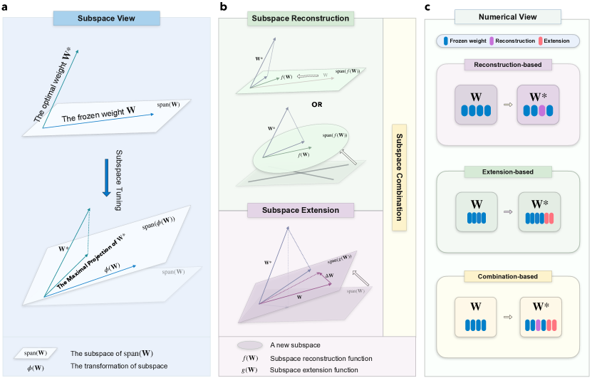
Figure 1: Framework of subspace tuning. a, Subspace tuning endeavors to identify the maximal projection of the optimal weight $\mathbf{W}^{*}$ onto the subspace spanned by the bases of $\phi(\mathbf{W})$. Here, $\phi(\mathbf{W})$ denotes the subspace transformation of the original frozen weight $\mathbf{W}$. b, Subspace reconstruction involves rescaling the subspace of $\mathbf{W}$ to approximate $\mathbf{W}^{*}$, or to construct a new subspace derived from the original. Subspace extension seeks to adjust the subspace of the original weight $\mathbf{W}$ such that it approaches or even encompasses $\mathbf{W}^{*}$. Subspace combination encompasses both the reconstruction and extension of subspaces. c, A numerical perspective on subspace tuning. Reconstruction involves modifying the original frozen parameters, while extension entails adding new tunable parameters.

We will briefly introduce each category and explore the underlying mathematical principles of corresponding methods. The full details are left to Methods. To simplify the notations for the following sections, let $\mathbf{A}\in\mathbb{R}^{n\times r}$ and $\mathbf{B}\in\mathbb{R}^{r\times m}$ ($r\ll n,m$) be two matrices that map the subspace to different dimensions, with the rank being $r$. $\mathbf{D}\in\mathbb{R}^{n\times m}$ represents a (rectangular) diagonal matrix. For a specific matrix $\mathbf{W}_{0}\in\mathbb{R}^{n\times m}$, we use $\mathbf{W}_{0}^{\dagger}$ to represent its Moore-Penrose pseudo-inverse, and $\mathbf{U}_{0}\in\mathbb{R}^{n\times n}$ and $\mathbf{V}_{0}\in\mathbb{R}^{m\times m}$ to represent its left and right singular vectors from the SVD decomposition, with $\mathbf{\Sigma}_{0}\in\mathbb{R}^{n\times m}$ being the corresponding singular values. All the notations are included in Table 1.

Table 1: Summary of major notations.

Notation	Mathematical Meanings
$\mathcal{P}(\cdot)$	The performance of a model
$\mathbf{W}\in\mathbb{R}^{n\times m}$	Frozen weight matrix
$\phi(\cdot)$	Subspace transformation function
$f(\cdot)$	Subspace reconstruction function
$g(\cdot)$	Subspace extension function
$\mathbf{A}\in\mathbb{R}^{n\times r}$	Down projection matrix
$\mathbf{B}\in\mathbb{R}^{r\times m}$	Up projection matrix
$\mathbf{D}\in\mathbb{R}^{n\times m}$	(Rectangle) Diagonal matrix
$\mathbf{W}^{\dagger}\in\mathbb{R}^{m\times n}$	Moore-Penrose Pseudo-inverse of a matrix $\mathbf{W}\in\mathbb{R}^{n\times m}$
$\mathbf{U}\in\mathbb{R}^{n\times n}$	Left singular vectors
$\mathbf{V}\in\mathbb{R}^{m\times m}$	Right singular vectors
$\mathbf{\Sigma}\in\mathbb{R}^{n\times m}$	Singular values

3 Subspace Reconstruction

Building upon the framework outlined previously, methods leveraging subspace reconstruction initiate by segmenting the space of $\mathbf{W}$ into interpretable subspaces. These subspaces are then refined to improve model efficiency. For these methods, the transformation function $\phi(\cdot)$ is succinctly expressed as $\phi(\mathbf{W})=f(\mathbf{W})$. Numerous PEFT strategies concentrate on directly reconstructing the subspaces related to the original weight matrix. Prominent examples include SAM-PARSER (Peng et al. (2024)), Diff Pruning (Guo et al. (2020)), (IA)³ (Liu et al. (2022)), BitFit (Zaken et al. (2021)), Prefix-tuning (Li and Liang (2021)), and Prompt-tuning (Lester et al. (2021)), etc.

We commence by exploring the Singular Value Decomposition (SVD), a pivotal technique in subspace decomposition. The original weight matrix $\mathbf{W}$ is decomposed into orthogonal subspaces that together encompass the entirety of the original matrix space. This decomposition is formally represented as $\mathbf{W}=\mathbf{U}\mathbf{\Sigma}\mathbf{V}$, where $\mathbf{\Sigma}\in\mathbb{R}^{n\times m}$ is a rectangle diagonal matrix given by:

$$\mathbf{\Sigma}=\begin{bmatrix}\Sigma_{11}&0&\cdots&0&0&\cdots&0\\ 0&\Sigma_{22}&\cdots&0&0&\cdots&0\\ \vdots&\vdots&\ddots&\vdots&\vdots&\ddots&\vdots\\ 0&0&\cdots&\Sigma_{nn}&0&\cdots&0\end{bmatrix}.$$ (3)

This decomposition systematically partitions $\mathbf{W}$ into three principal components:

• $\mathbf{U}$: Left Singular Vectors, which form orthonormal bases for the column space of $\mathbf{W}$.

• $\mathbf{\Sigma}$: Singular Values, represented by diagonal elements that measure the strength or significance of each principal axis and modify the dimensionality and scaling within the subspace.

• $\mathbf{V}$: Right Singular Vectors, constituting orthonormal bases for the row space of $\mathbf{W}$.

SVD elucidates the fundamental subspaces that underpin the structure of $\mathbf{W}$, allowing for the reconstruction of the original space by adeptly adjusting the subspaces acquired through the decomposition process. The refinement of these subspaces is delineated into three distinct modes (Fig. 2a and 2b):

• Mode 1, Singular Value Adjustment: This mode entails the modification of the singular values in $\mathbf{\Sigma}$, thereby adjusting the scaling within the respective principal subspaces. Altering these values modifies the significance attributed to each principal component, without affecting the directional properties of the subspaces defined by $\mathbf{U}$ and $\mathbf{V}$.

• Mode 2, Simple Singular Vector Adjustment: This mode involves straightforward adjustments to the singular vectors in $\mathbf{U}$ and $\mathbf{V}$ by scaling the subspaces they span. It preserves the directional characteristics of the subspaces while modifying their magnitudes to enhance performance.

• Mode 3, Complex Singular Vector Adjustment: This mode encompasses more intricate transformations of the singular vectors, involving reorientation or reshaping of the subspaces. It impacts both the direction and the scale of the subspaces, facilitating a comprehensive adjustment of the matrix structure.

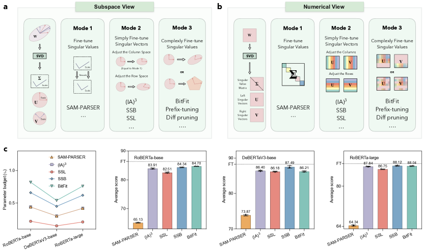
Figure 2: a, Subspace view of reconstruction-based methods. Fine-tuning the singular values involves rescaling the weights, while fine-tuning the singular vectors effectively reconstructs the subspace. b. Numerical view of reconstruction-based methods. We correspond adjustments in the subspace directly to their numerical adjustments. c, The performance of reconstruction-based methods. With less than 0.1% of the parameters of the pretrained model, SSL and SSB can achieve up to 99% of the performance of fully fine-tuning. The horizontal dashed line parallel to the x-axis, labeled FT, represents the performance of full fine-tuning. The average scores of each method are evaluated with three large pretrained models, RoBERTa-base (Liu et al. (2019)), DeBERTaV3-base (He et al. (2021b)), and RoBERTa-large (Liu et al. (2019)) on the GLUE benchmark. Error bars represent the standard error of the mean across five runs.

3.1 Mode 1 Reconstruction: Singular Value Adjustment

Mode 1 methods operate under the premise that the optimal weight matrix $\mathbf{W}^{*}$ and the original weight matrix $\mathbf{W}$ share identical bases for their row and column spaces. Consequently, their SVD decomposition is characterized by the same singular vectors $\mathbf{U}$ and $\mathbf{V}$. Given this assumption, the SVD composition of $\mathbf{W}^{*}$ can be expressed as

$$\mathbf{W}^{*}=\mathbf{U}\mathbf{\Sigma}^{*}\mathbf{V}^{\mathsf{T}},$$ (4)

where $\mathbf{\Sigma}^{*}$ represents the singular values that are optimized for the desired configuration. This formulation suggests that pinpointing the appropriate singular values for the optimal subspace is a direct and feasible approach, and this is what SAM-PARSER (Peng et al. (2024)) actually does.

This method is designed to reconstruct the parameter space by optimizing singular values. According to the original paper (Peng et al. (2024)), SAM-PARSER selectively targets the weight matrix associated with the ‘neck’ component of the SAM architecture (Kirillov et al. (2023)). This ‘neck’ component typically comprises two $256\times 256$ layers. They assert that adjusting merely 512 singular values within this structure can achieve performance levels comparable to other established baselines.

However, the practicality and efficacy of this method are potentially limited by its foundational assumptions. The presupposition that the subspaces derived from the singular vectors of $\mathbf{W}$ are congruent with those of $\mathbf{W}^{*}$ is a significant conjecture that may not consistently hold in real-world applications. Moreover, aligning the original subspace to the optimal weight’s subspace merely by scaling poses substantial challenges. Consequently, under equivalent conditions, the performance of the Mode 1 method is anticipated to lag considerably behind that of other techniques. Results in Fig. 2c (Supplementary Tables 2-4) proves that this method is substantially inferior to alternative approaches, even when allowed a larger parameter budget.

3.2 Mode 2 Reconstruction: Simple Singular Vector Adjustment

Shifting our focus from adjusting singular values, we now turn our attention to manipulating the subspaces defined by the singular vectors, i.e., Mode 2. Initially, we will concentrate on scaling the subspaces, which can be applied to the column or row spaces of the singular vectors. This is formally represented as:

$$\mathcal{T}(\mathbf{U})=\mathbf{U}\mathbf{D}\ {\rm or}\ \mathbf{D}\mathbf{U},$$ (5)

where $\mathcal{T}(\cdot)$ denotes the subspace scaling function and $\mathbf{D}$ is a diagonal matrix.

3.2.1 Scale the Column Space

If we scale the column space of singular vectors by assigning distinct weights to each vector, we define the transformations as $\mathcal{T}_{1}(\mathbf{U})=\mathbf{U}\mathbf{D}_{1}$ and $\mathcal{T}_{2}(\mathbf{V})=\mathbf{V}\mathbf{D}_{2}$, where $\mathbf{D}_{1}\in\mathbb{R}^{n\times n}$ and $\mathbf{D}_{2}\in\mathbb{R}^{m\times m}$ are diagonal matrices. The reconstructed weight matrix $\hat{\mathbf{W}}$ can then be obtained as:

$$\hat{\mathbf{W}} =\mathcal{T}_{1}(\mathbf{U})\mathbf{\Sigma}\mathcal{T}_{2}(\mathbf{V}^{\mathsf{T}})$$ (6)

$$=\mathbf{U}\mathbf{D}_{1}\mathbf{\Sigma}\mathbf{D}_{2}\mathbf{V}^{\mathsf{T}}$$

$$=\mathbf{U}\hat{\mathbf{\Sigma}}\mathbf{V}^{\mathsf{T}},$$

where $\hat{\mathbf{\Sigma}}=\mathbf{D}_{1}\mathbf{\Sigma}\mathbf{D}_{2}$. Therefore, scaling the column space of singular vectors is essentially an adjustment of the singular values.

3.2.2 Scale the Row Space

We can also apply distinct weights to each row of the singular vectors, defined as $\mathcal{T}_{1}(\mathbf{U})=\mathbf{D}_{1}\mathbf{U}$ and $\mathcal{T}_{2}(\mathbf{V})=\mathbf{D}_{2}\mathbf{V}$. Consequently, the reconstructed weight matrix $\hat{\mathbf{W}}$ is articulated as follows:

$$\hat{\mathbf{W}} =\mathcal{T}_{1}(\mathbf{U})\mathbf{\Sigma}\mathcal{T}_{2}(\mathbf{V}^{\mathsf{T}})$$ (7)

$$=\mathbf{D}_{1}\mathbf{U}\mathbf{\Sigma}\mathbf{V}^{\mathsf{T}}\mathbf{D}_{2}$$

$$=\mathbf{D}_{1}\mathbf{W}\mathbf{D}_{2}.$$

Thus, scaling the row space spanned by the left and right singular vectors essentially corresponds to scaling both the row and column spaces of the original weight matrix.

From this perspective, some methods can yield more in-depth explanations, such as (IA)³ (Liu et al. (2022)). In the original paper (Liu et al. (2022)), this method seeks to directly modify the activations within the model by introducing a learnable vector $\mathbf{l}\in\mathbb{R}^{m}$ to rescale the original weight matrix. The transformation is implemented via the Hadamard product $\odot$, represented as $\mathbf{l}\odot\mathbf{W}$. However, it can equivalently be expressed as $\mathbf{W}\mathbf{D}_{2}$, where $\mathbf{D}_{2}\in\mathbb{R}^{m\times m}$ is a diagonal matrix. Consequently, this approach actually scales the subspace of the right singular vectors, thereby reconstructing the original weight matrix $\mathbf{W}$.

The results in Fig. 2c demonstrate that merely scaling the subspace of the right singular vectors, i.e., (IA)³, can achieve performance comparable to fully fine-tuning. This insight naturally gives rise to an additional adjustment method: Scaling the Subspace of the Left singular vectors (SSL). If the dimensions of the subspaces spanned by both left and right singular vectors are comparable, the performance of SSL and (IA)³ are expected to be similar, since both methods enhance model adaptation by scaling a singular subspace. This is corroborated by the results shown in Fig. 2c (Supplementary Tables 2-4).

Further expanding on this concept, we introduce the method of Scaling the Subspace of Both left and right singular vectors (SSB). Theoretically, SSB should outperform both SSL and (IA)³ as it simultaneously scales both subspaces, potentially enhancing the reconstruction quality beyond the capabilities of single-subspace scaling. Results from Fig. 2c and detailed in Supplementary Tables 2-4, indicate that SSB is significantly superior to SSL and (IA)³. Additionally, while training fewer than one-thousandth of the parameters, SSB closely approximates the outcomes of fully fine-tuning.

Overall, these findings underscore the effectiveness of the adjustments specified in equation (7), confirming the potential of subspace scaling.

3.3 Mode 3 Reconstruction: Complex Singular Vector Adjustment

Mode 3 methods allow for more complicated transformations of the subspace spanned by singular vectors, with the form as $\mathcal{T}_{1}(\mathbf{U})=\mathbf{U}\mathbf{T}_{1}$ and $\mathcal{T}_{2}(\mathbf{V})=\mathbf{V}\mathbf{T}_{2}$, where $\mathbf{T}_{1}\in\mathbb{R}^{n\times n}$ and $\mathbf{T}_{2}\in\mathbb{R}^{m\times m}$ are two arbitrary matrices. Furthermore, $\mathcal{T}_{1}$ and $\mathcal{T}_{2}$ for nonlinear transformations are also allowed in Mode 3. These transformations can effectively convert the linear subspaces spanned by singular vectors into new nonlinear subspaces. In practice, we can achieve this by directly altering specific elements of $\mathbf{W}$. Representative methods include BitFit derivatives (Zaken et al. (2021); Lawton et al. (2023)), soft prompt derivatives (Li and Liang (2021); Lester et al. (2021)) and others (Guo et al. (2020); Sung et al. (2021); Das et al. (2023); Gheini et al. (2021); He et al. (2023); Liao et al. (2023)).

3.3.1 BitFit Derivatives

BitFit (Zaken et al. (2021)) is designed to optimize solely the bias terms within a model while keeping all other parameters frozen, achieving performance comparable to full fine-tuning. Extending this concept, S-BitFit (Lawton et al. (2023)) integrates Network Architecture Search (NAS) with the BitFit strategy, maintaining the structural integrity of BitFit by imposing constraints on the NAS algorithm to determine whether the gradient of the bias term should be zero.

We consider the scenario of fine-tuning the bias term of a layer. For an input $\mathbf{x}\in\mathbb{R}^{l\times n}$ with frozen weights $\mathbf{W}$ and bias term $\mathbf{b}\in\mathbb{R}^{m}$, the output of the layer is computed as follows:

$${\rm output}=\mathbf{xW}+\mathbf{1}_{l}\mathbf{b}^{\mathsf{T}},$$ (8)

where $\mathbf{1}_{l}\in\mathbb{R}^{l}$ is an all-one vector. To facilitate the integration of the bias term into the weight matrix, we can augment $\mathbf{W}$ by appending $\mathbf{b}^{\mathsf{T}}$ as an additional row. This alteration leads to the following representation:

$${\rm output}=\begin{bmatrix}\mathbf{x}&\mathbf{1}\end{bmatrix}\begin{bmatrix}\mathbf{W}\\ \mathbf{b}^{\mathsf{T}}\end{bmatrix}=\hat{\mathbf{x}}\hat{\mathbf{W}},$$ (9)

where $\mathbf{1}\in\mathbb{R}^{l}$ and $\hat{\mathbf{W}}\in\mathbb{R}^{(n+1)\times m}$ is the augmented matrix. Therefore, BitFit fundamentally involves fine-tuning each element of the final row of $\hat{\mathbf{W}}$, corresponding directly to reconstructing the row space of the augmented weight matrix.

3.3.2 Soft Prompt Derivatives

Soft prompt derivatives, such as Prefix-tuning (Li and Liang (2021)), and prompt-tuning (Lester et al. (2021)), are prevailing in natural language processing (Gao et al. (2020); Tan et al. (2021)). Prefix-tuning introduces trainable continuous tokens, or prefixes, appended to either the input or output of a layer. These prefixes, sourced from a specific parameter matrix, remain trainable while other parameters of the pre-trained model are fixed during training. Conversely, Prompt-tuning simplifies this approach by incorporating soft prompts solely at the input layer. These prompts also originate from an independent parameter matrix and are updated exclusively through gradient descent. Both methods preserve the original model parameters, providing benefits in low-data scenarios and demonstrating potential for generalization across various tasks.

Focusing on the design rather than specific layers to place prefixes, we consider a general case where for an input $\mathbf{x}\in\mathbb{R}^{l\times n}$ and the output $\mathbf{xW}$. $l$ learnable vectors $\mathbf{P}\in\mathbb{R}^{l\times m}$, known as soft prompts, are concatenated in the following formulation:

$${\rm concat}(\mathbf{P},\mathbf{xW})=\begin{bmatrix}\mathbf{P}\\ \mathbf{xW}\end{bmatrix}.$$ (10)

Similar to the approach used for BitFit, we can augment the weight matrix to restate equation (10) as

$$\begin{bmatrix}\mathbf{P}\\ \mathbf{xW}\end{bmatrix}=\begin{bmatrix}\mathbf{I}&\mathbf{0}_{l\times n}\\ \mathbf{0}_{l\times l}&\mathbf{x}\end{bmatrix}\begin{bmatrix}\mathbf{P}\\ \mathbf{W}\end{bmatrix}=\hat{\mathbf{x}}\hat{\mathbf{W}}.$$ (11)

Here, $\mathbf{I}\in\mathbb{R}^{l\times l}$ is the identity matrix, $\mathbf{0}_{l\times n}\in\mathbb{R}^{l\times n}$ and $\mathbf{0}_{l\times l}\in\mathbb{R}^{l\times}$ are zero matrices, and $\hat{\mathbf{W}}\in\mathbb{R}^{(n+l)\times m}$ is the augmented matrix. Thus, soft prompt derivatives essentially involve adjusting the elements of the initial several rows of the augmented weight matrix $\hat{\mathbf{W}}$, thereby reconstructing the original subspace.

3.3.3 Others

There are also methods that adjust the singular vectors by directly modifying elements within the original weight matrix, such as Diff pruning (Guo et al. (2020)), FishMask (Sung et al. (2021)), Fish-Dip (Das et al. (2023)), Xattn Tuning (Gheini et al. (2021)), SPT (He et al. (2023)), and PaFi (Liao et al. (2023)), etc.

4 Subspace Extension

Extension-based methods introduce a new subspace, incorporating the bases of this new subspace alongside those of the original weight matrix $\mathbf{W}$ to span an expanded space. These methods aim to find the closest projection of the optimal weight $\mathbf{W}^{*}$ within this new space, essentially seeking to broaden the basis of the original subspace to cover a larger dimensional area (Fig. 3). Generally, the transformation function for these methods is typically defined succinctly as $\phi(\mathbf{W})=g(\mathbf{W})=\mathbf{W}+s\Delta\mathbf{W}$, where $s$ represents a scaling factor. Here $\Delta\mathbf{W}$ corresponds to the introduced new subspace, which is also referred to as the addition term.

Considering the general case where the weight matrix $\mathbf{W}$ in $\mathbb{R}^{n\times m}$ and assuming $n\leq m$ without loss of generality. Ideally, we have $\phi(\mathbf{W})=\mathbf{W}^{*}$. This setup implies that $\mathbf{W}+s\Delta\mathbf{W}$ and $\mathbf{W}^{*}$occupy the same row and column spaces, positioning them within the same hyperplane. Ideally, if the rank of $\mathbf{W}$ is $n$, the dimension of its column space also equals $n$, allowing it to span the subspace $\mathbb{R}^{n}$. However, if the rank of $\mathbf{W}$ is less than $n$, it can only span a subspace within $\mathbb{R}^{n}$. Since we do not know the basis of the column space of $\mathbf{W}^{*}$, a conservative assumption is that the bases of the column spaces of $\Delta\mathbf{W}$ and $\mathbf{W}$ can span the entire $\mathbb{R}^{n}$ space. In the optimal scenario, the column basis vectors of $\Delta\mathbf{W}$ should ideally complement those of $\mathbf{W}$, implying that the column space of $\mathbf{W}^{*}$ represents the direct sum of these spaces.

Despite these factors, some studies suggest that the optimal weights $\mathbf{W}^{*}$ amplify certain directions within the original weight matrix which are task-specific but not crucial for pretraining (Hu et al. (2021)). Additionally, the optimal weights also adjust the major directions of $\mathbf{W}$ (Zhang and Pilanci (2024)). These insights imply that $\mathbf{W}^{*}$ likely shares a substantial subset of common bases with the subspace of $\mathbf{W}$. Therefore, $\Delta\mathbf{W}$ may only need to account for a small subset of bases absent in $\mathbf{W}$ but present in $\mathbf{W}^{*}$, allowing $\Delta\mathbf{W}$ to be a low-rank matrix (Hu et al. (2021); Si et al. (2024c)). Furthermore, empirical research demonstrates that full-parameter fine-tuning of pre-trained models can often be reparameterized into optimizations within a low-dimensional subspace (Aghajanyan et al. (2020); Li et al. (2018)), indicating that the optimal weights vary within this constrained, low-rank subspace. This low-rank characteristic of $\Delta\mathbf{W}$ underscores the basis for parameter efficiency in extension-based methods. We will show that regardless of the method employed, they all impose a low-rank constraint on $\Delta\mathbf{W}$.

An additional critical aspect is the scaling factor $s$. For extension-based methods, our objective is to determine the maximal projection of $\mathbf{W}^{*}$ within the hyperplane formed by $\mathbf{W}$ and $\Delta\mathbf{W}$, ensuring that $\mathbf{W}+s\Delta\mathbf{W}$ aligns as closely as possible with $\mathbf{W}^{*}$. Given fixed $\mathbf{W}$ and $\Delta\mathbf{W}$, only one value of $s$ will align the direction of $\mathbf{W}+s\Delta\mathbf{W}$ with that of $\mathbf{W}^{*}$. Therefore, the value of $s$ can have a significant or even critical impact on the performance.

There are two prominent series of extension-based methods within parameter-efficient tuning. The first series, known as LoRA derivatives, includes developments such as LoRA (Hu et al. (2021)), AdaLoRA (Zhang et al. (2022)), TriLoRA (Feng et al. (2024)), FLoRA (Si et al. (2024c)), VeRA (Kopiczko et al. (2023)), and LoTR (Bershatsky et al. (2024)). These methods primarily rely on low-rank matrix decomposition techniques. The second series, the Adapter derivatives, comprises methods such as those introduced by Houlsby et al. (Houlsby et al. (2019)), He et al. (He et al. (2021a)), and introduced by (Pfeiffer et al. (2020)), which incorporate small-scale neural modules, or adapters, into existing architectures.

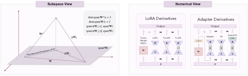
Figure 3: Subspace and Numerical views of extension-based methods. Extension-based methods introduce an additional weight matrix and then try to find the optimal weight projection within the subspace spanned by this additional weight and the original weight. To achieve this, the basis of the subspace constructed by the additional matrix should complement the basis of the original weights as much as possible. The right figure lists some common extension-based methods and their operations on matrices.

4.1 LoRA Derivatives

Building on the hypothesis that the change in weight matrices exhibits low-rank characteristics (Aghajanyan et al. (2020); Li et al. (2018)), LoRA introduces an addition term represented as $\Delta\mathbf{W}=\mathbf{A}\mathbf{B}$, where $\mathbf{A}\in\mathbb{R}^{n\times r}$ and $\mathbf{B}\in\mathbb{R}^{r\times m}$, and $r\ll\{n,m\}$. This approach aims to enhance parameter efficiency by exploiting the low-rank structure. Without loss of generality, assuming both $\mathbf{A}$ and $\mathbf{B}$ fully utilize the carrying capacities of their low ranks, i.e., ${\rm rank}(\mathbf{A})={\rm rank}(\mathbf{B})=r$. The addition term in LoRA aligns with the principles of full rank decomposition (Piziak and Odell (1999)). Subsequent research has introduced variants employing different decomposition strategies, such as TriLoRA (Feng et al. (2024)) and AdaLoRA (Zhang et al. (2022)), which utilize SVD decomposition (Eckart and Young (1936)) to formulate $\Delta\mathbf{W}=\mathbf{ADB}$ with $\mathbf{D}\in\mathbb{R}^{r\times r}$ being diagonal. Additionally, FLoRA (Si et al. (2024c)) implements a variation where $\Delta\mathbf{W}=\mathbf{AGB}$, with $\mathbf{G}\in\mathbb{R}^{r\times r}$ as an arbitrary matrix.

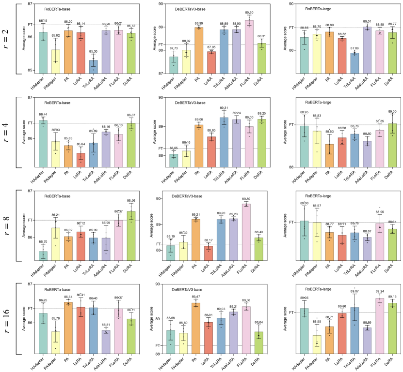
Figure 4: Average score of extension and combination-based methods. Each method is assessed under four different ranks. The horizontal dashed line parallel to the x-axis, labeled FT, represents the performance of full fine-tuning. In general the performance of FLoRA is superior to that of AdaLoRA and TriLoRA, followed by LoRA, and the performance of DoRA is superior to that of LoRA. The average scores of PEFT methods are evaluated with three large pretrained models, RoBERTa-base (Liu et al. (2019)), DeBERTaV3-base (He et al. (2021b)), and RoBERTa-large (Liu et al. (2019)) on the GLUE benchmark. Each method is assessed under four different ranks 2, 4, 8 and 16. Error bars represent the standard error of the mean across five runs.

From the perspective of matrix decomposition, these addition terms can be transformed into each other, as

$$\mathbf{AGB}=\mathbf{{AU}\Sigma{VB}}\ (\mathbf{G}=\mathbf{U\Sigma V})$$ (12)

$$= {\mathbf{A}^{\diamond}\mathbf{D}}\mathbf{B}^{\diamond}\ (\mathbf{A}^{\diamond}=\mathbf{AU},\mathbf{B}^{\diamond}=\mathbf{VB})$$

$$= \mathbf{A}^{*}\mathbf{B}^{\diamond}\ \ \ \ (\mathbf{A}^{*}=\mathbf{A}^{\diamond}\mathbf{D}).$$

Nevertheless, despite their structural similarities, these configurations result in varying levels of effectiveness. The effectiveness hierarchy is demonstrated as $\mathcal{P}(\mathbf{AGB})>\mathcal{P}(\mathbf{ADB})>\mathcal{P}(\mathbf{AB})$ in general, as evidenced by Fig. 4 (Supplementary Tables 2-4) and studies such as (Zhang et al. (2022); Hu et al. (2021); Feng et al. (2024); Si et al. (2024c)). Indeed, beyond the methods mentioned, despite the potential for various methods to be theoretically interchangeable in form, there are still significant performance differences which can be observed between them. Therefore, we introduce the following proposition:

Proposition 1.

The learning capability of extension-based methods is directly influenced by the decomposition form of $\Delta\mathbf{W}$, rather than by its mathematical equivalence to other forms.

This proposition is intriguing: If various forms are interchangeable and they all only apply the same low-rank constraint on $\Delta\mathbf{W}$, why do we still see differences in performance? Could a $\Delta\mathbf{W}$ learned by FLoRA for a specific weight not be equivalently learned by other methodologies such as LoRA and TriLoRA? This paradox highlights a deeper mystery in extension-based methods — beyond mere theoretical equivalence and the low-rank characteristics traditionally focused on, how exactly does each decomposition form impact the model’s learning dynamics?

To delve into this issue, let $\Delta\mathbf{W}^{*}=\mathbf{W}^{*}-\mathbf{W}$ represent the true alternations. In general, the addition term can be represented as $\Delta\mathbf{W}=\mathbf{AGB}$, where $\mathbf{G}$ can be configured as an arbitrary matrix, a diagonal matrix, or even an identity matrix. Ideally, $\mathbf{A}\mathbf{G}\mathbf{B}=\Delta\mathbf{W}^{*}$, and we have $\mathbf{G}=\mathbf{A}^{\dagger}\Delta\mathbf{W}^{*}\mathbf{B}^{\dagger}$. To delve deeper into the scenario where $\mathbf{G}$ is a diagonal matrix, we utilize SVD on $\Delta\mathbf{W}^{*}$, resulting in the following expression:

$$\mathbf{G}=\mathbf{A}^{\dagger}\mathbf{U}\mathbf{\Sigma}\mathbf{V}^{T}\mathbf{B}^{\dagger}$$ (13)

Given that $\mathbf{G}$ is a diagonal matrix, we simply constrain $\mathbf{A}^{\dagger}$ and $\mathbf{B}^{\dagger}$ as

$$\mathbf{A}^{\dagger} =\mathbf{D}_{1}\mathbf{U}^{\mathsf{T}}$$ (14)

$$\mathbf{B}^{\dagger} =\mathbf{V}\mathbf{D}_{2},$$

where $\mathbf{D}_{1}\in\mathbb{R}^{r\times n}$ and $\mathbf{D}_{2}\in\mathbb{R}^{m\times r}$ are rectangular diagonal matrices. This setup inversely dictates the formulations for $\mathbf{A}$ and $\mathbf{B}$ based on the pseudo-inverses of $\mathbf{D}_{1}$ and $\mathbf{D}_{2}$, as shown

$$\mathbf{A} =\mathbf{U}\mathbf{D}_{1}^{\dagger}$$ (15)

$$\mathbf{B} =\mathbf{D}_{2}^{\dagger}\mathbf{V}^{\mathsf{T}}.$$

This analysis reveals that $\mathbf{A}$ and $\mathbf{B}$ must be structured as linear combinations of the columns of $\mathbf{U}$ and $\mathbf{V}$, respectively. Consequently, the matrix relationships are captured as follows:

$$\mathbf{A}\mathbf{A}^{\mathsf{T}}=\mathbf{U}\mathbf{D}_{1}^{\dagger}\mathbf{D}_{1}^{\dagger\mathsf{T}}\mathbf{U}^{\mathsf{T}}, \ \ \mathbf{A}^{\mathsf{T}}\mathbf{A}=\mathbf{D}_{1}^{\dagger\mathsf{T}}\mathbf{D}_{1}^{\dagger},$$ (16)

$$\mathbf{B}^{\mathsf{T}}\mathbf{B}=\mathbf{V}\mathbf{D}_{2}^{\dagger\mathsf{T}}\mathbf{D}_{2}^{\dagger}\mathbf{V}^{\mathsf{T}}, \ \ \mathbf{B}\mathbf{B}^{\mathsf{T}}=\mathbf{D}_{2}^{\dagger}\mathbf{D}_{2}^{\dagger\mathsf{T}}.$$

By simplifying the constraints on $\mathbf{D}_{1}=\mathbf{I}_{r\times n}\in\mathbb{R}^{r\times n}$ and $\mathbf{D}_{2}=\mathbf{I}_{m\times r}\in\mathbb{R}^{m\times r}$ during training, the following identities hold:

$$\mathbf{D}_{1}^{\dagger\mathsf{T}}\mathbf{D}_{1}^{\dagger}=\mathbf{D}_{2}^{\dagger}\mathbf{D}_{2}^{\dagger\mathsf{T}}=\mathbf{I}_{r\times r}.$$ (17)

In this configuration, $\mathbf{D}_{1}^{\dagger}\mathbf{D}_{1}^{\dagger\mathsf{T}}$ and $\mathbf{D}_{2}^{\dagger\mathsf{T}}\mathbf{D}_{2}^{\dagger}$ function as block diagonal identity matrices. This arrangement introduces a degree of semi-orthogonality to both $\mathbf{A}$ and $\mathbf{B}$, since $\mathbf{A}^{\mathsf{T}}\mathbf{A}=\mathbf{B}\mathbf{B}^{\mathsf{T}}=\mathbf{I}_{r\times r}$ and $\mathbf{A}\mathbf{A}^{\mathsf{T}}$ and $\mathbf{B}^{\mathsf{T}}\mathbf{B}$ are arbitrary matrices. Therefore, the SVD form of $\Delta\mathbf{W}$ applied in AdaLoRA introduces semi-orthogonality constraints on matrices $\mathbf{A}$ and $\mathbf{B}$ during model training, which regulates the learning dynamics.

Extending this further, when $\mathbf{G}$ is an identity matrix, we obtain

$$\mathbf{I}=\mathbf{A}^{\dagger}\Delta\mathbf{W}^{*}\mathbf{B}^{\dagger}=\mathbf{D}_{1}\mathbf{\Sigma}\mathbf{D}_{2}.$$ (18)

It becomes evident that $\mathbf{D}_{1}$ and $\mathbf{D}_{2}$ are intricately correlated. Therefore, we may conclude that it is feasible to designate one of the diagonal matrices, either $\mathbf{D}_{1}$ and $\mathbf{D}_{2}$, as an identity matrix during the training process. However, constraining the other matrix becomes more complex and less straightforward, due to the correlation and interdependence required in equation (18). Thus, in addition to the semi-orthogonality constraints, this form of $\Delta\mathbf{W}$ applied in LoRA also introduces direct correlations between $\mathbf{A}$ and $\mathbf{B}$, which complicates the model’s learning process.

Moreover, if $\mathbf{G}$ is an arbitrary matrix such as that used in FLoRA, it is obvious that there are no inherent constraints on $\mathbf{A}$ and $\mathbf{B}$ themselves, nor between them. This lack of constraints can make the model’s learning process more flexible and potentially easier, as it allows $\mathbf{A}$ and $\mathbf{B}$ to adapt independently without being restricted by rigid structural relationships.

At this point, we can explain why different decomposition forms yield varying levels of effectiveness in model training. When $\mathbf{G}$ is a diagonal matrix, the model is not only required to learn specific patterns within matrices $\mathbf{A}$ and $\mathbf{B}$ but also to ensure that these matrices maintain orthogonality. This dual requirement can complicate the learning process, as the model must adhere to these strict structural relationships while optimizing the weight adjustments. Moreover, if $\mathbf{G}$ is configured as an identity matrix, the model faces an additional challenge as it must further constrain the interrelationships between $\mathbf{A}$ and $\mathbf{B}$. These more stringent constraints can significantly increase the complexity of the learning task, potentially hindering the model’s ability to efficiently learn and adapt Conversely, by relaxing or eliminating the diagonal constraint on $\mathbf{G}$ during training, the model is afforded a simpler task environment. This relaxation increases the likelihood that the model can effectively learn the optimal $\Delta\mathbf{W}^{*}$ without being overly burdened by rigid structural stipulations. This leads us to propose the following:

Proposition 2.

Beyond the inherent low-rank constraint of the decomposition itself, different decomposition forms implicitly and subtly impose additional constraints on the matrix patterns. The fewer the constraints imposed on the matrix patterns by the decomposition, the better the model’s performance is likely to be.

Revisiting on our analytical reasoning, it is crucial to understand that a model’s learning capabilities and the accuracy of mathematical proofs are distinct aspects. When considering the capabilities of a model, we can facilitate its learning by simplifying the form of mathematical decompositions. This allows us to focus on practical training strategies without conflating them with the strict correctness often required in theoretical mathematics. For instance, in equation (14), we simply constrain $\mathbf{A}^{\dagger}$ and $\mathbf{B}^{\dagger}$ as the product of “a diagonal matrix” and an orthogonal matrix rather than “an arbitrary matrix“. In fact, even taking mathematical correctness into account, we set $\mathbf{A}^{\dagger}$ and $\mathbf{B}^{\dagger}$ as

$$\mathbf{A}^{\dagger}=\mathbf{P}\mathbf{U}^{\mathsf{T}},\mathbf{B}^{\dagger}=\mathbf{V}\mathbf{\Sigma}^{\dagger}\mathbf{Q},$$ (19)

where $\mathbf{P}\in\mathbb{R}^{r\times n}$ and $\mathbf{Q}\in\mathbb{R}^{n\times r}$ are arbitrary matrices. In this scenario, the decomposition form of LoRA dictates that $\mathbf{Q}$ must be the pseudo-inverse of $\mathbf{P}$. Building on this setup, AdaLoRA further specifies that each column of $\mathbf{Q}$, which is the pseudo-inverse of $\mathbf{P}$, may have distinct weights. Conversely, FLoRA does not impose any such constraints. We can still arrive at the same conclusion: LoRA imposes the most restrictions on the matrix patterns for model learning, followed by AdaLoRA, while FLoRA imposes the least.

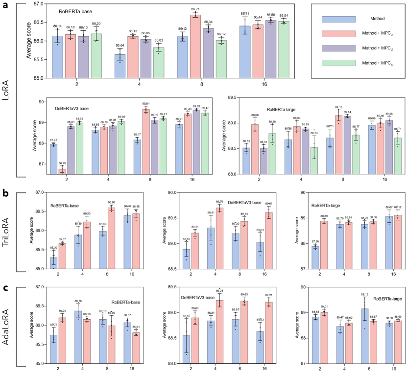
Figure 5: Average score of different methods coupled with MPC framework. a, The performance of LoRA when coupled with MPC_o, MPC_d, and MPC_n. b-c, The performance of TriLoRA and AdaLoRA when coupled with MPC_o, respectively. The MPC framework significantly enhances the performance of various PEFT methods, as evaluated with three large pretrained models, RoBERTa-base (Liu et al. (2019)), DeBERTaV3-base (He et al. (2021b)), and RoBERTa-large (Liu et al. (2019)) on the GLUE benchmark. Each method is assessed under four different ranks 2, 4, 8 and 16. Error bars represent the standard error of the mean across five runs.

4.2 The Inspiration Gained: MPC Framework

The analysis of different decompositions in the LoRA derivatives provides valuable insights into optimizing model performance through matrix interactions. Specifically, structuring the learning process to emphasize specific interactions between these matrices can greatly enhance the model’s efficiency and accuracy.

When the matrix $\mathbf{G}$ is diagonal, such as AdaLoRA and TriLoRA, to facilitate the model’s ability to learn specific patterns in $\mathbf{A}$ and $\mathbf{B}$, a semi-orthogonality regularizer term can be introduced as:

$$\min\|\mathbf{A}^{\mathsf{T}}\mathbf{A}-\mathbf{I}\|_{F}^{2}+\|\mathbf{B}\mathbf{B}^{\mathsf{T}}-\mathbf{I}\|_{F}^{2}.$$ (20)

However, based on the previous analysis, the situation changes if $\mathbf{G}$ is an identity matrix (such as LoRA). In such cases, $\mathbf{D}_{1}$ and $\mathbf{D}_{2}$ are highly correlated, and we can constrain one of $\mathbf{A}$ and $\mathbf{B}$ to exhibit orthogonality, such as $\mathbf{A}$. For the other matrix $\mathbf{B}$, we can adopt two types of constraints: one is constraining $\mathbf{B}$ also to exhibit orthogonality, with the regularizer formulated in the equation (20). This constraint assumes that $\mathbf{\Sigma}$ is an identity matrix, which makes it a more aggressive approach. In contrast, the other constraint is relatively conservative. We only require $\mathbf{B}\mathbf{B}^{\mathsf{T}}$ to be a diagonal matrix. The corresponding regularization term would then be:

$$\min\|\mathbf{A}^{\mathsf{T}}\mathbf{A}-\mathbf{I}\|_{F}^{2}+\|\mathbf{B}\mathbf{B}^{\mathsf{T}}-{\rm diag}(\mathbf{B}\mathbf{B}^{\mathsf{T}})\|_{F}^{2}.$$ (21)

Additionally, we can directly sever the connection between matrices $\mathbf{A}$ and $\mathbf{B}$ to alleviate the constraints during the learning process. This can be achieved by introducing a non-linear operation between the matrix multiplications of $\mathbf{A}$ and $\mathbf{B}$, effectively breaking the strong link that typically exists between them. Overall, we unify the aforementioned three Matrix Pattern Constraints as a novel framework termed as MPC, with MPC_o (equation (20)), MPC_d (equation (21)) and MPC_n (nonlinear involvement). Without introducing additional parameters, MPC effectively enhance the performance of existing LoRA derivatives, as shown in Figs. 5a-5c (Supplementary Tables.2-4). Moreover, MPC can help different methods achieve more stable training. Methods combined with MPC generally exhibit smaller standard deviations compared to those without MPC.

4.3 Adapter Derivatives

Adapter derivatives (Houlsby et al. (2019); Pfeiffer et al. (2020); He et al. (2021a)) represent another class of extension-based methods. These adapters, which mainly consist of a down-projection followed by an up-projection, modify only specific parts of the model during training. For an input $\mathbf{x}\in\mathbb{R}^{n\times m}$, the adapters are integrated with a residual connection, resulting in the final transformation:

$$\mathbf{x}\rightarrow\mathbf{x}+h(\mathbf{xA})\mathbf{B},$$ (22)

where $h(\cdot)$ is a nonlinear activation function, $\mathbf{A}\in\mathbb{R}^{m\times r}$ and $\mathbf{B}\in\mathbb{R}^{r\times m}$. This configuration can be further expressed by considering the weight matrix as the input $\hat{\mathbf{W}}=\mathbf{x}\in\mathbb{R}^{n\times m}$ and a hypothetical input $\hat{\mathbf{x}}=\mathbf{I}\in\mathbb{R}^{m\times m}$ as

$$\hat{\mathbf{W}}\hat{\mathbf{x}}\rightarrow\hat{\mathbf{W}}\hat{\mathbf{x}}+h(\hat{\mathbf{W}}\mathbf{A})\mathbf{B}\hat{\mathbf{x}},$$ (23)

Therefore, the addition term introduced by the Adapter can be formulated as $\Delta\mathbf{W}=h(\hat{\mathbf{W}}\mathbf{A})\mathbf{B}$. Following a similar analysis to LoRA, we can derive

$$h(\hat{\mathbf{W}}\mathbf{A})=\Delta\mathbf{W}^{*}\mathbf{B}^{\dagger}.$$ (24)

Compared with LoRA, where $\mathbf{A}=\Delta\mathbf{W}^{*}\mathbf{B}^{\dagger}$, the Adapter’s inclusion of a nonlinear activation layer further reduces the constraints on learning the relationships between $\mathbf{A}$ and $\mathbf{B}$. According to Proposition 2, this reduction in constraints should lead to better model performance. However, the input to the Adapter is fixed as $\mathbf{I}$, which implies that Adapters can only be placed at specific modules within a backbone architecture, potentially limiting their overall effectiveness.

Subsequent developments, such as the MAM Adapter (He et al. (2021a)), which includes the PA or Scaled PA, adopt a parallel architecture similar to LoRA to configure adapter layers. This configuration allows Adapters to be applied to any weight matrix within the model. We focus particularly on the design of the PA and its application across various model positions. Specifically, for an input $\mathbf{x}\in\mathbf{R}^{d\times n}$, we have

$$\mathbf{x}\mathbf{W}\rightarrow\mathbf{x}\mathbf{W}+h(\mathbf{xA})\mathbf{B},$$ (25)

where $\mathbf{A}\in\mathbb{R}^{n\times r}$ and $\mathbf{B}\in\mathbb{R}^{r\times m}$. Following equation (23), we have

$$\hat{\mathbf{W}}\hat{\mathbf{x}}\rightarrow\hat{\mathbf{W}}\hat{\mathbf{x}}+h(\hat{\mathbf{W}}\mathbf{A})\mathbf{B},$$ (26)

resulting in $\Delta\mathbf{W}=h(\hat{\mathbf{W}}\mathbf{A})\mathbf{B}\hat{\mathbf{x}}^{\dagger}$. According to Proposition 2, this nonlinear flexibility typically results in enhanced model performance, as evidenced by our experiments in Fig. 4.

5 Subspace Combination

Combination-based methods perform both subspace reconstruction and extension simultaneously, blending the principles of both approaches. Moreover, for some methods which can be categorized as both a reconstruction-based and an extension-based method, we also classify them as the combination-based methods. We here analyse several representative combination-based methods as follows.

DoRA (Liu et al. (2024)) first decomposes the model weights $\mathbf{W}$ into two parts: magnitude and direction. The process of adjusting these components is defined as follows:

$$\phi(\mathbf{W})=\mathbf{m}\frac{\mathbf{W}+\mathbf{AB}}{\|\mathbf{W}+\mathbf{AB}\|_{c}},$$ (27)

where $\mathbf{m}\in\mathbb{R}^{1\times m}$ represents the magnitude, and $\|\cdot\|_{c}$ is the vector-wise norm of a matrix applied across each column. Given that $\mathbf{m}$ is learnable during the training process, this formula can be simplified as:

$$\phi(\mathbf{W})=\mathbf{W}\mathbf{D}+\mathbf{ABD},$$ (28)

where $\mathbf{D}\in\mathbb{R}^{m\times m}$ is a diagonal matrix.

We focus on the extension $\Delta\mathbf{W}=\mathbf{ABD}$ while disregarding the transformation of the column space of $\mathbf{W}$. Following the analysis similar to that for LoRA derivatives, we can derive

$$\mathbf{I}=\mathbf{A}^{\dagger}\Delta\mathbf{W}^{*}\mathbf{D}^{\dagger}\mathbf{B}^{\dagger}=\mathbf{A}^{\dagger}\mathbf{U}\mathbf{\Sigma}\mathbf{V}^{\mathsf{T}}\mathbf{D}^{\dagger}\mathbf{B}^{\dagger}.$$ (29)

With the constraints $\mathbf{A}^{\dagger}=\mathbf{D}_{1}\mathbf{U}^{\mathsf{T}}$ and $\mathbf{D}^{\dagger}\mathbf{B}^{\dagger}=\mathbf{V}\mathbf{D}_{2}$, where $\mathbf{D}_{1}\in\mathbb{R}^{r\times n}$ and $\mathbf{D}_{2}\in\mathbb{R}^{m\times r}$ are rectangle diagonal, we have

$$\mathbf{I}=\mathbf{D}_{1}\mathbf{\Sigma}\mathbf{D_{2}},\ \mathbf{A}=\mathbf{U}\mathbf{D}_{1}^{\dagger},\ \mathbf{B}=\mathbf{D}_{2}^{\dagger}\mathbf{V}^{\mathsf{T}}\mathbf{D}^{\dagger}.$$ (30)

It is important to note

$$\mathbf{B}^{\mathsf{T}}\mathbf{B} =\mathbf{D}^{\dagger\mathsf{T}}\mathbf{V}\mathbf{D}_{2}^{\dagger\mathsf{T}}\mathbf{D}_{2}^{\dagger}\mathbf{V}^{\mathsf{T}}\mathbf{D}^{\dagger}$$ (31)

$$\mathbf{B}\mathbf{B}^{\mathsf{T}} =\mathbf{D}_{2}^{\dagger}\mathbf{V}^{\mathsf{T}}\mathbf{D}^{\dagger}\mathbf{D}^{\dagger\mathsf{T}}\mathbf{V}\mathbf{D}_{2}^{\dagger\mathsf{T}}.$$

Since ${\rm rank}(\mathbf{D}_{2}^{\dagger})=r$ and the matrix product $\mathbf{D}_{2}^{\dagger\mathsf{T}}\mathbf{D}_{2}^{\dagger}\in\mathbb{R}^{m\times m}$ cannot be an identity matrix, both $\mathbf{B}^{\mathsf{T}}\mathbf{B}$ and $\mathbf{B}\mathbf{B}^{\mathsf{T}}$ are arbitrary matrices. Therefore, DoRA can at most impose semi-orthogonal constraints on matrix $\mathbf{A}$, while matrix $\mathbf{B}$ remains unconstrained. Additionally, DoRA reconstructs $\mathbf{W}$ by scaling its column space. Based on Proposition 2, it is concluded that DoRA can lead to superior performance compared to LoRA, as shown in Fig. 4 and also noted in (Liu et al. (2024); Han et al. (2024)).

The Spectral Adapter (Zhang and Pilanci (2024)) is another innovative example within combination-based methods. Specifically, it starts by decomposing the weight matrix $\mathbf{W}$ into its SVD components $\mathbf{W}=\mathbf{U}\mathbf{\Sigma}\mathbf{V}^{\mathsf{T}}$. It then integrates trainable matrices $\mathbf{A}\in\mathbb{R}^{n\times r}$ and $\mathbf{B}\in\mathbb{R}^{m\times r}$ with the top r columns of $\mathbf{U}$ and $\mathbf{V}$, with the form as

$$\phi(\mathbf{W})=\begin{bmatrix}\mathbf{U}_{r}+\mathbf{A}&\mathbf{U}_{n-r}\end{bmatrix}\mathbf{\Sigma}\begin{bmatrix}\mathbf{V}_{r}+\mathbf{B}&\mathbf{V}_{n-r}\end{bmatrix}^{\mathsf{T}},$$ (32)

where $\mathbf{U}_{r}$ and $\mathbf{V}_{r}$ represent the top $r$ columns of $\mathbf{U}$ and $\mathbf{V}$, and $\mathbf{U}_{n-r}$ and $\mathbf{V}_{n-r}$ account for the remaining columns. The equation (32) can be rewritten as

$$\phi(\mathbf{W})=\mathbf{W}+\mathbf{A}\mathbf{\Sigma}\mathbf{V}^{\mathsf{T}}+\mathbf{U}\mathbf{\Sigma}\mathbf{B}^{\mathsf{T}}+\mathbf{A}\mathbf{\Sigma}\mathbf{B}.$$ (33)

Therefore, Spectral Adapter can also be viewed as introducing an additional term $\Delta\mathbf{W}=\mathbf{A}\mathbf{\Sigma}\mathbf{V}^{\mathsf{T}}+\mathbf{U}\mathbf{\Sigma}\mathbf{B}^{\mathsf{T}}+\mathbf{A}\mathbf{\Sigma}\mathbf{B}$.

SVDiff (Han et al. (2023)) modifies the singular values $\mathbf{\Sigma}$ of the original weight matrix $\mathbf{W}$ by incorporating a diagonal “spectral shift” matrix $\mathbf{D}$. This adjustment is formulated as follows:

$$\phi(\mathbf{W})=\mathbf{U}h(\mathbf{\Sigma}+\mathbf{D})\mathbf{V}^{\mathsf{T}},$$ (34)

where $\mathbf{U}$ and $\mathbf{V}$ represent the left and right singular vectors of $\mathbf{W}$, respectively, and $h(\cdot)$ denotes the nonlinear function ReLU. This equation can be expanded to

$$\phi(\mathbf{W}) =\mathbf{U}\mathbf{\Sigma}\mathbf{V}^{\mathsf{T}}+\mathbf{U}\ \mathcal{H}_{\mathbf{\Sigma}}(\mathbf{D})\mathbf{V}^{\mathsf{T}}$$ (35)

$$=\mathbf{W}+\Delta\mathbf{W}.$$

In this context, $\mathcal{H}_{\mathbf{A}}(\cdot)$ is an element-wise operator where $\mathcal{H}_{\mathbf{\Sigma}}(\mathbf{D})=[\max(D{ij},-\Sigma_{ij})]_{n\times m}$. Consequently, SVDiff not only reconstructs but also extends the subspace. Moreover, we can conclude that the approach, which selectively reconstructs the singular values or vectors by introducing additional trainable components rather than directly altering the singular components, can be categorized as a combination-based method.

6 Implementation Details

In our experiments, we employed three distinct scales of models: RoBERTa-base (Liu et al. (2019)), DeBERTaV3-base (He et al. (2021b)), and RoBERTa-Large (Liu et al. (2019)). We used the General Language Understanding Evaluation (GLUE) (Wang et al. (2018)) benchmark as our dataset, which comprises two single-sentence classification tasks, three similarity and paraphrase tasks, and four natural language inference tasks. Details of the GLUE dataset are provided in Supplementary Table 5.

The configurations and hyper-parameters for all methods were adopted according to their respective original publications. Specifically, (IA)³ was applied to the keys and values in both self-attention and encoder-decoder attention mechanisms, as well as to the intermediate activation of the position-wise feed-forward networks, along with SSL and SSB. Additionally, we set the rank $r$ values at 2, 4, 8, 16 for LoRA, TriLoRA, AdaLoRA, FLoRA, and DoRA, and align the parameter budgets of other methods as closely as possible with LoRA to ensure comparability across different approaches. These methods were applied to all linear layers. We conducted all baseline comparisons using the publicly available PyTorch implementation (Paszke et al. (2019)), and all experiments were performed on NVIDIA A100 GPUs. Results are reported as the mean of 5 runs with different random seeds to ensure the reliability and reproducibility of our findings. The hyper-parameters for different experiments are shown in Supplementary Table 6.

7 Discussion

The adaptation of pre-trained foundation models for a diverse array of downstream tasks has become a ubiquitous practice in artificial intelligence. Given the extensive range of tasks and the prohibitive costs associated, it is impractical to adjust all parameters comprehensively. In response, the development of parameter-efficient fine-tuning techniques (PEFT) has emerged, facilitating updates to the pre-trained model weights in a manner that is significantly more resource-efficient. Although methods of PEFT continue to proliferate, a comprehensive understanding of their underlying mathematical principles and the variance in their performance remains elusive. Therefore, in this work, we take the first step by conceptualizing all PEFT methods from a decomposition perspective, unifying them under the subspace tuning methodology. The mathematical foundations underlying each PEFT method are dissected, identifying that each represents a distinct manipulation of the subspace. Inspired by theoretical insights, we propose two novel PEFT methods. Extensive experiments show that by training less than one thousandth of the parameters, can approximate the effects of full fine-tuning.

Furthermore, we elucidate the reasons behind the performance disparities among different methods. Our analysis yields significant conclusions. The comparative analysis of various PEFT strategies such as LoRA, AdaLoRA, and FLoRA, reveals distinct patterns in their efficacy during training. The more stringent the matrix pattern learning, the more the model performance is constrained. We tested the performance of nearly ten algorithms on three different large pretrained models under four levels of parameter budgets, validating our conclusions with more than 3800 experimental runs. Based on this analysis, we propose a framework that enhances the learning of matrix patterns during model training. The effectiveness of this framework has been confirmed through more than 2000 experimental runs across three methods, four parameter budgets, and three large pretrained models.

The significance of our findings extends beyond the immediate scope of parameter-efficient fine-tuning. The principles underlying PEFT methods can be extrapolated to other domains of artificial intelligence, such as transfer learning (Mudrakarta et al. (2018); Houlsby et al. (2019)), multi-task learning (Liu et al. (2023); Mahabadi et al. (2021)), fast training (Mahabadi et al. (2021); Rücklé et al. (2020)), and also areas where computational resources are a limiting factor, such as real-time systems (Jovanovic and Voss (2024)) and embedded devices (Feng and Narayanan (2023)). By analyzing the theoretical aspects of PEFT methods in different scenarios, we can comprehend the underlying logic and, based on these theoretical insights, refine these methods to further enhance their impact across related fields. Additionally, the theoretical underpinnings of subspace tuning present intriguing possibilities for further exploration in this domain as well as others, potentially catalyzing advancements and influencing developments across the broader artificial intelligence landscape.

8 Conclusion

In this paper, we unify all PEFT methods from the perspective of decomposition for the first time and explain the operations of different methods at the subspace level. We provide a detailed analysis of the mathematical principles behind each method and explain why their performance varies. Additionally, we propose two new methods that can achieve 99% of the performance with less than one-thousandth of the training parameters. We also introduce a framework that can help existing algorithms effectively enhance their performance. Overall, this work shows considerable potential for further development in this field and related areas, and we hope that the related paradigms can be further explored through theoretical and experimental research.

Appendix A Extended Data

Table 2: Results with RoBERTa-base (Liu et al. (2019)) fine-tuned on GLUE development set.

Row	Method	‰Params	MNLI	SST-2	CoLA	QQP	QNLI	RTE	MRPC	STS-B	All
			Acc	Acc	Mcc	Acc	Acc	Acc	Acc	Corr	Avg.
1	Fully FT	1000‰	87.62	94.84	63.58	91.87	92.80	78.80	90.20	91.23	86.37
2	SAM-PARSER	0.44‰	54.92	85.09	39.85	75.92	70.79	59.57	74.26	60.65	65.13
3	(IA)3	0.44‰	84.83	94.15	60.14	87.92	90.39	76.17	87.75	90.23	83.91
4	SSL	0.22‰	83.45	93.81	56.02	87.30	89.20	74.01	86.76	89.52	82.51
5	SSB	0.66‰	85.80	94.61	60.92	88.65	91.20	76.53	86.76	90.23	84.34
6	BitFit	0.82‰	85.29	94.61	59.58	88.10	91.20	79.78	88.73	90.32	84.70
7	HAdapter	2.50‰	87.45	94.72	63.88	90.29	92.71	80.14	89.22	90.80	86.15
8	PAdapter	2.43‰	87.11	94.15	62.74	89.95	92.71	80.14	87.99	90.13	85.62
9	PA	2.65‰	87.55	94.38	64.23	90.03	92.81	80.51	89.22	90.85	86.20
10	LoRA	2.65‰	87.20	94.38	65.61	89.25	92.07	81.59	87.99	91.01	86.14
11	LoRA + MPCo	2.65‰	86.96	94.72	64.08	89.24	92.00	81.23	90.20	91.03	86.18
12	LoRA + MPCd	2.65‰	87.03	94.50	64.24	89.19	92.13	81.51	89.46	91.00	86.13
13	LoRA + MPCn	2.65‰	87.55	94.38	64.23	90.03	92.81	80.51	89.22	90.85	86.20
14	TriLoRA	2.65‰	86.81	94.61	64.47	89.61	91.82	76.53	88.24	90.31	85.30
15	TriLoRA + MPCo	2.65‰	87.48	94.27	63.97	89.93	92.55	78.34	88.24	90.55	85.67
16	AdaLoRA - MPCo	2.65‰	87.51	94.15	62.35	90.14	92.97	80.51	87.75	90.62	85.75
17	AdaLoRA	2.65‰	87.31	94.72	64.33	89.77	92.81	81.95	88.24	90.48	86.20
18	FLoRA	2.65‰	87.31	94.38	64.09	89.97	92.77	82.67	87.75	90.77	86.21
19	DoRA	3.32‰	86.74	94.50	66.19	90.28	91.95	79.78	88.48	91.01	86.12
20	HAdapter	4.87‰	87.34	94.95	63.68	90.55	92.81	81.23	89.71	91.21	86.44
21	PAdapter	4.80‰	87.22	94.84	64.91	89.95	92.38	79.06	88.75	90.31	85.93
22	PA	5.31‰	87.32	94.27	62.43	90.26	92.68	79.42	89.22	91.07	85.83
23	LoRA	5.31‰	87.13	94.38	62.52	89.40	92.20	79.42	88.97	91.11	85.64
24	LoRA + MPCo	5.31‰	87.02	94.38	64.58	89.47	92.33	81.23	88.97	91.02	86.13
25	LoRA + MPCd	5.31‰	87.15	94.27	63.68	89.44	92.44	81.59	88.73	91.08	86.05
26	LoRA + MPCn	5.31‰	87.32	94.27	62.43	90.26	92.68	79.42	89.22	91.07	85.83
27	TriLoRA	5.31‰	87.45	93.81	63.85	90.30	92.42	80.14	88.97	90.17	85.89
28	TriLoRA + MPCo	5.31‰	87.90	94.84	62.20	90.24	92.60	83.03	88.73	90.26	86.23
29	AdaLoRA - MPCo	5.31‰	87.39	94.50	63.52	90.12	92.64	82.31	89.71	90.83	86.38
30	AdaLoRA	5.31‰	87.43	94.50	61.74	89.76	92.90	82.67	89.71	90.55	86.16
31	FLoRA	5.31‰	87.59	93.92	62.13	90.28	92.73	82.67	88.73	90.78	86.10
32	DoRA	5.97‰	87.06	94.38	66.19	90.67	92.15	80.87	88.73	90.94	86.37
33	HAdapter	9.59‰	87.74	94.04	61.53	89.27	92.57	80.14	89.46	90.84	85.70
34	PAdapter	9.52‰	86.90	94.50	66.52	90.05	92.46	80.87	88.24	90.13	86.21
35	PA	10.62‰	87.50	94.61	62.89	89.51	92.73	80.87	89.46	90.59	86.02
36	LoRA	10.62‰	87.38	94.84	64.58	89.39	92.47	80.14	89.21	90.96	86.12
37	LoRA + MPCo	10.62‰	87.50	94.61	65.38	89.55	93.19	83.03	89.22	91.21	86.71
38	LoRA + MPCd	10.62‰	87.31	94.84	64.43	89.41	92.57	82.31	88.73	91.09	86.34
39	LoRA + MPCn	10.62‰	87.50	94.61	62.89	89.51	92.73	80.87	89.46	90.59	86.02
40	TriLoRA	10.62‰	87.44	94.84	62.91	90.70	92.82	80.14	88.73	90.37	85.99
41	TriLoRA + MPCo	10.62‰	87.97	94.72	65.06	90.38	93.01	81.95	89.22	90.51	86.60
42	AdaLoRA - MPCo	10.62‰	87.31	94.61	62.45	90.17	92.88	82.31	88.73	90.82	86.16
43	AdaLoRA	10.62‰	87.13	94.61	62.61	89.49	92.62	81.95	88.97	90.53	85.99
44	FLoRA	10.64‰	87.43	94.27	63.31	90.38	92.75	81.59	90.44	90.82	86.37
45	DoRA	11.28‰	87.14	94.50	66.06	91.02	92.13	81.95	88.73	90.96	86.56
46	HAdapter	19.03‰	87.31	94.72	63.91	90.80	92.49	79.78	89.95	91.00	86.25
47	PAdapter	18.96‰	86.64	94.84	64.55	90.22	92.73	76.17	90.44	90.66	85.78
48	PA	21.24‰	87.55	94.50	65.79	90.93	92.68	80.87	89.22	90.74	86.54
49	LoRA	21.24‰	87.49	94.27	64.70	89.39	92.33	81.59	90.44	91.03	86.41
50	LoRA + MPCo	21.24‰	87.44	94.95	62.62	89.48	93.15	82.67	90.20	90.99	86.44
51	LoRA + MPCd	21.24‰	87.34	94.50	65.33	89.26	92.82	83.03	88.97	91.22	86.56
52	LoRA + MPCn	21.24‰	87.55	94.50	65.79	90.93	92.68	80.87	89.22	90.74	86.54
53	TriLoRA	21.24‰	87.54	94.50	64.72	90.98	92.93	80.87	88.73	90.93	86.40
54	TriLoRA + MPCo	21.24‰	88.21	94.61	62.89	90.53	93.01	82.67	88.97	90.67	86.45
55	AdaLoRA - MPCo	21.24‰	87.32	94.61	62.41	90.19	92.90	81.59	88.97	90.57	86.07
56	AdaLoRA	21.24‰	86.93	94.50	61.56	89.30	92.62	82.31	88.97	90.30	85.81
57	FLoRA	21.38‰	87.64	94.95	65.17	90.90	92.53	79.78	89.71	90.75	86.37
58	DoRA	21.90‰	86.98	94.61	65.30	90.92	92.90	78.70	88.48	91.00	86.11

Table 3: Results with DeBERTaV3-base (He et al. (2021b)) fine-tuned on GLUE development set.

Row	Method	‰Params	MNLI	SST-2	CoLA	QQP	QNLI	RTE	MRPC	STS-B	All
			Acc	Acc	Mcc	Acc	Acc	Acc	Acc	Corr	Avg.
1	Fully FT	1000‰	89.90	95.63	69.19	92.40	94.03	83.75	89.46	91.60	88.24
2	SAM-PARSER	0.30‰	68.32	84.28	55.21	81.91	75.86	66.06	76.47	82.82	73.87
3	(IA)3	0.30‰	89.44	95.52	67.01	89.01	91.80	79.42	88.23	90.79	86.40
4	SSL	0.15‰	88.35	95.07	66.64	88.19	90.10	82.31	88.68	90.13	86.18
5	SSB	0.45‰	89.86	95.53	67.82	89.87	93.41	83.75	88.72	90.94	87.49
6	BitFit	0.54‰	89.37	94.84	66.96	88.41	92.24	78.80	87.75	91.35	86.21
7	HAdapter	1.68‰	90.10	95.41	67.65	91.19	93.52	83.39	89.25	91.31	87.73
8	PAdapter	1.63‰	89.89	94.72	69.06	91.05	93.87	84.48	89.71	91.38	88.02
9	PA	1.79‰	90.24	95.64	71.24	91.40	94.25	87.36	90.20	91.57	88.99
10	LoRA	1.79‰	90.03	93.92	69.15	90.61	93.37	85.56	90.19	90.75	87.95
11	LoRA + MPCo	1.79‰	89.99	93.61	68.87	86.95	91.87	85.71	89.70	87.33	86.75
12	LoRA + MPCd	1.79‰	90.06	95.30	69.91	91.29	94.34	88.08	89.95	91.53	88.81
13	LoRA + MPCn	1.79‰	90.24	95.64	71.24	91.40	94.25	87.36	90.20	91.57	88.99
14	TriLoRA	1.79‰	90.32	95.87	69.61	91.38	94.25	87.00	91.17	91.48	88.89
15	TriLoRA + MPCo	1.79‰	90.39	95.87	70.00	91.38	94.25	88.09	92.16	91.53	89.21
16	AdaLoRA - MPCo	1.79‰	90.34	95.10	69.51	90.98	94.10	87.01	89.95	91.40	88.55
17	AdaLoRA	1.79‰	90.40	95.80	69.98	91.43	94.23	87.36	90.43	91.63	88.90
18	FLoRA	1.79‰	90.60	96.00	70.20	91.40	94.46	88.81	90.93	91.96	89.30
19	DoRA	2.23‰	90.21	94.38	69.33	90.84	93.26	86.94	90.19	91.34	88.31
20	HAdapter	3.32‰	90.12	95.30	67.87	91.30	93.76	85.56	89.22	91.30	88.05
21	PAdapter	3.26‰	90.15	95.53	69.48	91.27	93.98	84.12	89.22	91.52	88.16
22	PA	3.61‰	90.23	96.11	69.78	91.77	94.27	88.08	90.20	92.03	89.06
23	LoRA	3.61‰	89.90	94.15	68.87	91.16	93.59	89.89	90.19	91.46	88.65
24	LoRA + MPCo	3.61‰	89.92	95.06	69.55	92.10	93.66	87.72	90.93	91.34	88.79
25	LoRA + MPCd	3.61‰	89.93	95.18	69.82	92.13	93.92	87.73	90.44	91.65	88.85
26	LoRA + MPCn	3.61‰	90.23	96.11	69.78	91.77	94.27	88.08	90.20	92.03	89.06
27	TriLoRA	3.61‰	90.37	96.10	70.87	91.88	94.51	88.45	90.93	91.42	89.31
28	TriLoRA + MPCo	3.61‰	90.55	96.10	72.37	91.93	94.55	88.45	92.16	91.52	89.70
29	AdaLoRA - MPCo	3.61‰	90.40	95.76	69.86	91.40	94.53	87.00	90.20	91.58	88.84
30	AdaLoRA	3.61‰	90.27	95.76	69.58	91.47	94.65	89.53	91.42	91.23	89.24
31	FLoRA	3.61‰	90.23	95.76	70.72	91.44	94.20	87.36	90.93	91.35	89.00
32	DoRA	4.06‰	90.12	96.22	68.24	91.55	94.65	89.53	92.40	91.29	89.25
33	HAdapter	6.63‰	90.13	95.53	68.64	91.27	94.11	84.48	89.95	91.48	88.19
34	PAdapter	6.41‰	90.33	95.61	68.77	91.40	94.29	85.20	89.46	91.54	88.32
35	PA	7.23‰	90.18	95.99	70.69	91.80	94.34	88.81	90.20	91.68	89.21
36	LoRA	7.23‰	89.80	93.69	69.30	91.78	92.97	85.70	90.68	91.62	88.17
37	LoRA + MPCo	7.23‰	90.60	95.64	72.19	92.29	93.75	89.53	91.17	91.91	89.64
38	LoRA + MPCd	7.23‰	90.20	95.53	70.06	92.23	93.78	88.81	90.20	91.99	89.10
39	LoRA + MPCn	7.23‰	90.18	95.99	70.69	91.80	94.34	88.81	90.20	91.68	89.21
40	TriLoRA	7.23‰	90.28	95.99	68.28	91.97	94.47	89.53	91.67	91.43	89.20
41	TriLoRA + MPCo	7.23‰	90.60	96.10	70.78	91.96	94.51	89.17	90.93	91.49	89.44
42	AdaLoRA - MPCo	7.23‰	90.38	95.99	69.12	91.36	94.23	87.72	90.93	91.20	88.87
43	AdaLoRA	7.23‰	90.38	95.87	71.45	91.19	94.36	88.09	90.69	91.84	89.23
44	FLoRA	7.24‰	90.82	96.21	72.05	91.94	94.60	89.53	91.18	92.04	89.80
45	DoRA	7.66‰	89.67	94.61	69.08	91.80	93.23	87.33	90.68	91.73	88.49
46	HAdapter	12.93‰	89.81	95.41	69.96	92.25	94.09	86.28	89.70	91.93	88.68
47	PAdapter	12.88‰	89.82	94.84	70.69	92.31	94.09	86.28	89.21	91.54	88.60
48	PA	14.43‰	90.35	95.64	71.45	92.30	94.38	88.81	90.93	91.89	89.47
49	LoRA	14.43‰	89.49	93.78	71.61	92.33	93.92	87.36	91.17	91.63	88.91
50	LoRA + MPCo	14.43‰	90.32	95.98	72.26	92.30	93.73	88.08	91.17	91.61	89.43
51	LoRA + MPCd	14.43‰	90.33	95.64	72.99	92.51	94.16	89.53	90.20	91.61	89.62
52	LoRA + MPCn	14.43‰	90.35	95.64	71.45	92.30	94.38	88.81	90.93	91.89	89.47
53	TriLoRA	14.43‰	90.20	95.87	68.64	92.25	94.36	88.81	90.69	91.39	89.03
54	TriLoRA + MPCo	14.43‰	90.59	96.22	72.71	92.15	94.62	88.08	90.93	91.56	89.61
55	AdaLoRA - MPCo	14.43‰	90.23	96.10	68.49	90.72	94.31	87.72	90.20	91.30	88.63
56	AdaLoRA	14.43‰	90.21	95.87	72.83	90.87	94.47	87.72	90.44	91.23	89.21
57	FLoRA	14.52‰	90.09	95.87	70.71	91.67	94.47	89.53	90.93	91.58	89.36
58	DoRA	14.87‰	90.17	93.92	69.92	92.47	93.21	87.00	90.68	91.73	88.64

Table 4: Results with RoBERTa-large (Liu et al. (2019)) fine-tuned on GLUE development set.

Row	Method	‰Params	MNLI	SST-2	CoLA	QQP	QNLI	RTE	MRPC	STS-B	All
			Acc	Acc	Mcc	Acc	Acc	Acc	Acc	Corr	Avg.
1	Fully FT	1000‰	90.29	96.41	68.02	92.24	94.74	86.66	90.92	92.44	88.97
2	SAM-PARSER	0.42‰	52.43	87.50	42.24	76.28	66.47	60.29	75.25	54.27	64.34
3	(IA)3	0.42‰	90.11	95.99	67.01	89.55	93.28	89.17	88.97	88.60	87.84
4	SSL	0.21‰	89.55	95.87	66.92	89.07	92.24	86.64	87.50	86.19	86.75
5	SSB	0.62‰	90.38	95.64	67.26	90.19	93.78	88.45	89.46	89.82	88.12
6	BitFit	0.76‰	90.15	96.22	68.53	89.50	94.12	84.15	89.95	91.68	88.04
7	HAdapter	2.35‰	90.66	96.22	67.25	90.82	94.78	86.28	90.20	92.30	88.56
8	PAdapter	2.29‰	90.39	96.22	67.25	90.47	94.47	88.44	89.95	92.38	88.70
9	PA	2.49‰	90.79	96.33	66.91	90.91	94.80	87.73	90.44	92.46	88.80
10	LoRA	2.49‰	90.41	95.99	67.83	90.75	94.05	87.72	89.46	91.92	88.52
11	LoRA + MPCo	2.49‰	90.73	96.33	68.10	91.01	94.55	88.80	89.95	92.36	88.98
12	LoRA + MPCd	2.49‰	90.50	96.33	65.29	91.15	94.60	86.64	91.18	92.38	88.51
13	LoRA + MPCn	2.49‰	90.79	96.33	66.91	90.91	94.80	87.73	90.44	92.46	88.80
14	TriLoRA	2.49‰	90.12	95.87	65.53	90.58	93.68	85.20	90.69	91.43	87.89
15	TriLoRA + MPCo	2.49‰	90.85	96.10	68.96	90.96	94.87	88.45	89.46	91.45	88.89
16	AdaLoRA - MPCo	2.49‰	90.59	96.10	67.87	91.16	94.67	88.45	89.71	92.08	88.83
17	AdaLoRA	2.49‰	90.69	96.22	67.08	91.01	94.69	89.53	90.68	92.16	89.01
18	FLoRA	2.49‰	90.62	96.10	68.97	91.16	94.67	87.55	89.46	92.26	88.85
19	DoRA	3.12‰	90.60	96.22	66.62	91.23	94.47	88.08	90.93	92.00	88.77
20	HAdapter	4.57‰	90.64	96.44	67.51	91.13	94.65	88.08	90.93	92.21	88.95
21	PAdapter	4.50‰	90.31	96.22	68.17	89.84	94.51	88.44	90.93	92.21	88.83
22	PA	4.98‰	90.52	95.87	66.56	89.42	94.75	87.72	91.18	92.24	88.53
23	LoRA	4.98‰	90.68	96.10	68.36	91.16	94.60	85.20	90.93	92.43	88.68
24	LoRA + MPCo	4.98‰	90.68	95.99	68.95	91.30	94.58	86.64	91.42	92.35	88.94
25	LoRA + MPCd	4.98‰	90.72	96.21	69.55	91.20	94.47	86.28	90.44	92.27	88.89
26	LoRA + MPCn	4.98‰	90.52	95.87	66.56	89.42	94.75	87.72	91.18	92.24	88.53
27	TriLoRA	4.98‰	90.51	96.10	67.98	91.20	94.33	86.64	91.42	91.86	88.76
28	TriLoRA + MPCo	4.98‰	90.96	95.76	67.26	91.08	95.06	88.81	89.95	91.80	88.84
29	AdaLoRA - MPCo	4.98‰	90.65	96.22	66.03	91.24	94.86	86.28	90.44	92.05	88.47
30	AdaLoRA	4.98‰	90.86	95.76	65.39	90.91	94.87	89.17	89.95	91.87	88.60
31	FLoRA	4.99‰	90.41	95.99	69.19	91.16	94.55	87.73	89.71	92.04	88.85
32	DoRA	5.61‰	90.61	96.79	68.22	91.57	94.44	86.64	91.18	92.55	89.00
33	HAdapter	9.00‰	90.57	96.10	68.57	91.62	94.73	87.00	90.93	92.49	89.00
34	PAdapter	8.93‰	90.29	95.76	68.47	91.39	94.60	87.72	90.93	92.61	88.97
35	PA	9.97‰	90.44	96.67	66.93	91.03	94.91	87.00	90.93	92.23	88.77
36	LoRA	9.97‰	90.73	95.87	67.83	91.28	94.73	86.28	90.69	92.30	88.71
37	LoRA + MPCo	9.97‰	90.66	95.99	71.56	91.43	94.65	85.92	90.69	92.31	89.15
38	LoRA + MPCd	9.97‰	90.64	96.22	69.23	91.22	94.91	87.00	91.67	92.24	89.14
39	LoRA + MPCn	9.97‰	90.44	96.67	66.93	91.03	94.91	87.00	90.93	92.23	88.77
40	TriLoRA	9.97‰	90.41	96.67	68.01	91.46	94.58	86.64	89.95	92.35	88.76
41	TriLoRA + MPCo	9.97‰	90.86	96.10	66.76	91.15	95.08	88.08	90.93	91.91	88.86
42	AdaLoRA - MPCo	9.97‰	90.83	96.22	68.36	91.25	94.82	88.45	91.42	91.92	89.16
43	AdaLoRA	9.97‰	90.65	96.10	65.96	90.80	94.73	89.53	89.71	91.90	88.67
44	FLoRA	9.98‰	90.51	95.87	67.43	91.30	94.80	88.80	90.69	92.18	88.95
45	DoRA	10.59‰	90.67	95.99	66.87	91.69	94.75	87.00	91.42	92.30	88.84
46	HAdapter	17.87‰	90.42	96.10	67.32	91.65	94.78	89.89	89.71	92.50	89.05
47	PAdapter	17.80‰	90.38	94.84	67.70	91.60	94.67	88.44	88.48	92.30	88.55
48	PA	19.94‰	90.31	96.33	66.52	91.16	94.73	86.64	91.18	92.79	88.71
49	LoRA	19.94‰	90.69	95.87	68.36	91.35	94.62	88.08	90.69	92.05	88.96
50	LoRA + MPCo	19.94‰	90.77	96.10	68.74	91.44	94.97	87.73	89.95	92.27	89.00
51	LoRA + MPCd	19.94‰	90.77	96.33	68.57	91.20	94.69	87.73	90.69	92.52	89.06
52	LoRA + MPCn	19.94‰	90.31	96.33	66.52	91.16	94.73	86.64	91.18	92.79	88.71
53	TriLoRA	19.94‰	90.58	95.99	69.04	91.73	94.93	88.08	90.20	92.00	89.07
54	TriLoRA + MPCo	19.94‰	90.83	96.44	68.57	91.27	95.02	88.81	89.95	92.05	89.12
55	AdaLoRA - MPCo	19.94‰	90.64	96.33	65.83	91.39	94.86	87.73	90.20	91.84	88.60
56	AdaLoRA	19.94‰	90.50	95.87	65.34	90.53	94.98	90.25	90.20	91.83	88.69
57	FLoRA	19.98‰	90.61	96.10	70.16	90.57	94.76	89.53	89.95	92.24	89.24
58	DoRA	20.56‰	90.72	96.22	68.33	91.80	94.98	88.08	90.44	92.65	89.15

Table 5: Details of GLUE dataset.

Dataset	Task	# Train	# Dev	# Test	# Label	Metrics
Single-Sentence Classification
CoLA	Acceptability	8.5k	1k	1k	2	Matthews corr
SST	Sentiment	67k	872	1.8k	2	Accuracy
Pairwise Text Classification
MNLI	NLI	393k	20k	20k	3	Accuracy
RTE	NLI	2.5k	276	3k	2	Accuracy
QQP	Paraphrase	364k	40k	391k	2	Accuracy / F1
MRPC	Paraphrase	3.7k	408	1.7k	2	Accuracy / F1
QNLI	QA/ NLI	108k	5.7k	5.7k	2	Accuracy
Text Similarity
STS-B	Similarity	7k	1.5k	1.4k	1	Pearson/ Spearman Corr

Table 6: Hyper-parameter setup for GLUE benchmark.

Dataset	MNLI	RTE	QNLI	MRPC
learning rate	$5\times 10^{-4}$	$1.2\times 10^{-3}$	$1.2\times 10^{-3}$	$1\times 10^{-3}$
batch size	32	32	32	32
#epochs	7	50	5	30
Dataset	QQP	SST-2	CoLA	STS-B
learning rate	$5\times 10^{-4}$	$8\times 10^{-4}$	$5\times 10^{-4}$	$2.2\times 10^{-3}$
batch size	32	32	32	32
#epochs	5	24	25	25

Author Contributions

C. S. and W. S. conceived the project. C. S. performed all the theoretical analysis and experiments. C. S. wrote the paper. C. S. and W. S. checked the formulation and revised the paper. X. Y. supervised the project.

References

- Achiam et al. [2023] Josh Achiam, Steven Adler, Sandhini Agarwal, Lama Ahmad, Ilge Akkaya, Florencia Leoni Aleman, Diogo Almeida, Janko Altenschmidt, Sam Altman, Shyamal Anadkat, et al. Gpt-4 technical report. arXiv preprint arXiv:2303.08774, 2023.
- Aghajanyan et al. [2020] Armen Aghajanyan, Luke Zettlemoyer, and Sonal Gupta. Intrinsic dimensionality explains the effectiveness of language model fine-tuning. arXiv preprint arXiv:2012.13255, 2020.
- Bershatsky et al. [2024] Daniel Bershatsky, Daria Cherniuk, Talgat Daulbaev, and Ivan Oseledets. Lotr: Low tensor rank weight adaptation. arXiv preprint arXiv:2402.01376, 2024.
- Brown et al. [2020] Tom Brown, Benjamin Mann, Nick Ryder, Melanie Subbiah, Jared D Kaplan, Prafulla Dhariwal, Arvind Neelakantan, Pranav Shyam, Girish Sastry, Amanda Askell, et al. Language models are few-shot learners. Advances in neural information processing systems, 33:1877–1901, 2020.
- Chen et al. [2022] Shoufa Chen, Chongjian Ge, Zhan Tong, Jiangliu Wang, Yibing Song, Jue Wang, and Ping Luo. Adaptformer: Adapting vision transformers for scalable visual recognition. Advances in Neural Information Processing Systems, 35:16664–16678, 2022.
- Chen et al. [2024] Wei Chen, Zichen Miao, and Qiang Qiu. Parameter-efficient tuning of large convolutional models. arXiv preprint arXiv:2403.00269, 2024.
- Das et al. [2023] Sarkar Snigdha Sarathi Das, Ranran Haoran Zhang, Peng Shi, Wenpeng Yin, and Rui Zhang. Unified low-resource sequence labeling by sample-aware dynamic sparse finetuning. arXiv preprint arXiv:2311.03748, 2023.
- Devlin et al. [2018] Jacob Devlin, Ming-Wei Chang, Kenton Lee, and Kristina Toutanova. Bert: Pre-training of deep bidirectional transformers for language understanding. arXiv preprint arXiv:1810.04805, 2018.
- Ding et al. [2023] Ning Ding, Yujia Qin, Guang Yang, Fuchao Wei, Zonghan Yang, Yusheng Su, Shengding Hu, Yulin Chen, Chi-Min Chan, Weize Chen, et al. Parameter-efficient fine-tuning of large-scale pre-trained language models. Nature Machine Intelligence, 5(3):220–235, 2023.
- Eckart and Young [1936] Carl Eckart and Gale Young. The approximation of one matrix by another of lower rank. Psychometrika, 1(3):211–218, 1936.
- Feng et al. [2024] Chengcheng Feng, Mu He, Qiuyu Tian, Haojie Yin, Xiaofang Zhao, Hongwei Tang, and Xingqiang Wei. Trilora: Integrating svd for advanced style personalization in text-to-image generation. arXiv preprint arXiv:2405.11236, 2024.
- Feng and Narayanan [2023] Tiantian Feng and Shrikanth Narayanan. Peft-ser: On the use of parameter efficient transfer learning approaches for speech emotion recognition using pre-trained speech models. In 2023 11th International Conference on Affective Computing and Intelligent Interaction (ACII), pages 1–8. IEEE, 2023.
- Fischer et al. [2024] Marc Fischer, Alexander Bartler, and Bin Yang. Prompt tuning for parameter-efficient medical image segmentation. Medical Image Analysis, 91:103024, 2024.
- Francis [1961] John GF Francis. The qr transformation a unitary analogue to the lr transformation—part 1. The Computer Journal, 4(3):265–271, 1961.
- Fu et al. [2023] Zihao Fu, Haoran Yang, Anthony Man-Cho So, Wai Lam, Lidong Bing, and Nigel Collier. On the effectiveness of parameter-efficient fine-tuning. In Proceedings of the AAAI Conference on Artificial Intelligence, pages 12799–12807, 2023.
- Gao et al. [2020] Tianyu Gao, Adam Fisch, and Danqi Chen. Making pre-trained language models better few-shot learners. arXiv preprint arXiv:2012.15723, 2020.
- Gheini et al. [2021] Mozhdeh Gheini, Xiang Ren, and Jonathan May. Cross-attention is all you need: Adapting pretrained transformers for machine translation. arXiv preprint arXiv:2104.08771, 2021.
- Guo et al. [2020] Demi Guo, Alexander M Rush, and Yoon Kim. Parameter-efficient transfer learning with diff pruning. arXiv preprint arXiv:2012.07463, 2020.
- Han et al. [2023] Ligong Han, Yinxiao Li, Han Zhang, Peyman Milanfar, Dimitris Metaxas, and Feng Yang. Svdiff: Compact parameter space for diffusion fine-tuning. In Proceedings of the IEEE/CVF International Conference on Computer Vision, pages 7323–7334, 2023.
- Han et al. [2024] Zeyu Han, Chao Gao, Jinyang Liu, Sai Qian Zhang, et al. Parameter-efficient fine-tuning for large models: A comprehensive survey. arXiv preprint arXiv:2403.14608, 2024.
- He et al. [2023] Haoyu He, Jianfei Cai, Jing Zhang, Dacheng Tao, and Bohan Zhuang. Sensitivity-aware visual parameter-efficient fine-tuning. In Proceedings of the IEEE/CVF International Conference on Computer Vision, pages 11825–11835, 2023.
- He et al. [2021a] Junxian He, Chunting Zhou, Xuezhe Ma, Taylor Berg-Kirkpatrick, and Graham Neubig. Towards a unified view of parameter-efficient transfer learning. arXiv preprint arXiv:2110.04366, 2021a.
- He et al. [2021b] Pengcheng He, Jianfeng Gao, and Weizhu Chen. Debertav3: Improving deberta using electra-style pre-training with gradient-disentangled embedding sharing. arXiv preprint arXiv:2111.09543, 2021b.
- Houlsby et al. [2019] Neil Houlsby, Andrei Giurgiu, Stanislaw Jastrzebski, Bruna Morrone, Quentin De Laroussilhe, Andrea Gesmundo, Mona Attariyan, and Sylvain Gelly. Parameter-efficient transfer learning for nlp. In International conference on machine learning, pages 2790–2799. PMLR, 2019.
- Hu et al. [2021] Edward J Hu, Yelong Shen, Phillip Wallis, Zeyuan Allen-Zhu, Yuanzhi Li, Shean Wang, Lu Wang, and Weizhu Chen. Lora: Low-rank adaptation of large language models. arXiv preprint arXiv:2106.09685, 2021.
- Hyeon-Woo et al. [2021] Nam Hyeon-Woo, Moon Ye-Bin, and Tae-Hyun Oh. Fedpara: Low-rank hadamard product for communication-efficient federated learning. arXiv preprint arXiv:2108.06098, 2021.
- Jovanovic and Voss [2024] Mladjan Jovanovic and Peter Voss. Trends and challenges of real-time learning in large language models: A critical review. arXiv preprint arXiv:2404.18311, 2024.
- Karimi Mahabadi et al. [2021] Rabeeh Karimi Mahabadi, James Henderson, and Sebastian Ruder. Compacter: Efficient low-rank hypercomplex adapter layers. Advances in Neural Information Processing Systems, 34:1022–1035, 2021.
- Kirillov et al. [2023] Alexander Kirillov, Eric Mintun, Nikhila Ravi, Hanzi Mao, Chloe Rolland, Laura Gustafson, Tete Xiao, Spencer Whitehead, Alexander C Berg, Wan-Yen Lo, et al. Segment anything. In Proceedings of the IEEE/CVF International Conference on Computer Vision, pages 4015–4026, 2023.
- Kopiczko et al. [2023] Dawid Jan Kopiczko, Tijmen Blankevoort, and Yuki Markus Asano. Vera: Vector-based random matrix adaptation. arXiv preprint arXiv:2310.11454, 2023.
- Kublanovskaya [1962] Vera N Kublanovskaya. On some algorithms for the solution of the complete eigenvalue problem. USSR Computational Mathematics and Mathematical Physics, 1(3):637–657, 1962.
- Lawton et al. [2023] Neal Lawton, Anoop Kumar, Govind Thattai, Aram Galstyan, and Greg Ver Steeg. Neural architecture search for parameter-efficient fine-tuning of large pre-trained language models. arXiv preprint arXiv:2305.16597, 2023.
- Lester et al. [2021] Brian Lester, Rami Al-Rfou, and Noah Constant. The power of scale for parameter-efficient prompt tuning. arXiv preprint arXiv:2104.08691, 2021.
- Li et al. [2018] Chunyuan Li, Heerad Farkhoor, Rosanne Liu, and Jason Yosinski. Measuring the intrinsic dimension of objective landscapes. arXiv preprint arXiv:1804.08838, 2018.
- Li and Liang [2021] Xiang Lisa Li and Percy Liang. Prefix-tuning: Optimizing continuous prompts for generation. arXiv preprint arXiv:2101.00190, 2021.
- Liao et al. [2023] Baohao Liao, Yan Meng, and Christof Monz. Parameter-efficient fine-tuning without introducing new latency. arXiv preprint arXiv:2305.16742, 2023.
- Liu et al. [2022] Haokun Liu, Derek Tam, Mohammed Muqeeth, Jay Mohta, Tenghao Huang, Mohit Bansal, and Colin A Raffel. Few-shot parameter-efficient fine-tuning is better and cheaper than in-context learning. Advances in Neural Information Processing Systems, 35:1950–1965, 2022.
- Liu et al. [2023] Pengfei Liu, Weizhe Yuan, Jinlan Fu, Zhengbao Jiang, Hiroaki Hayashi, and Graham Neubig. Pre-train, prompt, and predict: A systematic survey of prompting methods in natural language processing. ACM Computing Surveys, 55(9):1–35, 2023.
- Liu et al. [2024] Shih-Yang Liu, Chien-Yi Wang, Hongxu Yin, Pavlo Molchanov, Yu-Chiang Frank Wang, Kwang-Ting Cheng, and Min-Hung Chen. Dora: Weight-decomposed low-rank adaptation. arXiv preprint arXiv:2402.09353, 2024.
- Liu et al. [2019] Yinhan Liu, Myle Ott, Naman Goyal, Jingfei Du, Mandar Joshi, Danqi Chen, Omer Levy, Mike Lewis, Luke Zettlemoyer, and Veselin Stoyanov. Roberta: A robustly optimized bert pretraining approach. arXiv preprint arXiv:1907.11692, 2019.
- Luo et al. [2023] Gen Luo, Minglang Huang, Yiyi Zhou, Xiaoshuai Sun, Guannan Jiang, Zhiyu Wang, and Rongrong Ji. Towards efficient visual adaption via structural re-parameterization. arXiv preprint arXiv:2302.08106, 2023.
- Ma et al. [2024] Jun Ma, Yuting He, Feifei Li, Lin Han, Chenyu You, and Bo Wang. Segment anything in medical images. Nature Communications, 15(1):654, 2024.
- Mahabadi et al. [2021] Rabeeh Karimi Mahabadi, Sebastian Ruder, Mostafa Dehghani, and James Henderson. Parameter-efficient multi-task fine-tuning for transformers via shared hypernetworks. arXiv preprint arXiv:2106.04489, 2021.
- Mao et al. [2023] Rui Mao, Guanyi Chen, Xulang Zhang, Frank Guerin, and Erik Cambria. Gpteval: A survey on assessments of chatgpt and gpt-4. arXiv preprint arXiv:2308.12488, 2023.
- Mudrakarta et al. [2018] Pramod Kaushik Mudrakarta, Mark Sandler, Andrey Zhmoginov, and Andrew Howard. K for the price of 1: Parameter-efficient multi-task and transfer learning. arXiv preprint arXiv:1810.10703, 2018.
- Paszke et al. [2019] Adam Paszke, Sam Gross, Francisco Massa, Adam Lerer, James Bradbury, Gregory Chanan, Trevor Killeen, Zeming Lin, Natalia Gimelshein, Luca Antiga, et al. Pytorch: An imperative style, high-performance deep learning library. Advances in neural information processing systems, 32, 2019.
- Peng et al. [2024] Zelin Peng, Zhengqin Xu, Zhilin Zeng, Xiaokang Yang, and Wei Shen. Sam-parser: Fine-tuning sam efficiently by parameter space reconstruction. In Proceedings of the AAAI Conference on Artificial Intelligence, pages 4515–4523, 2024.
- Pfeiffer et al. [2020] Jonas Pfeiffer, Aishwarya Kamath, Andreas Rücklé, Kyunghyun Cho, and Iryna Gurevych. Adapterfusion: Non-destructive task composition for transfer learning. arXiv preprint arXiv:2005.00247, 2020.
- Piziak and Odell [1999] Robert Piziak and Patrick L Odell. Full rank factorization of matrices. Mathematics magazine, 72(3):193–201, 1999.
- Qiu et al. [2020] Xipeng Qiu, Tianxiang Sun, Yige Xu, Yunfan Shao, Ning Dai, and Xuanjing Huang. Pre-trained models for natural language processing: A survey. Science China Technological Sciences, 63(10):1872–1897, 2020.
- Qiu et al. [2023] Zeju Qiu, Weiyang Liu, Haiwen Feng, Yuxuan Xue, Yao Feng, Zhen Liu, Dan Zhang, Adrian Weller, and Bernhard Schölkopf. Controlling text-to-image diffusion by orthogonal finetuning. Advances in Neural Information Processing Systems, 36:79320–79362, 2023.
- Radford et al. [2019] Alec Radford, Jeffrey Wu, Rewon Child, David Luan, Dario Amodei, Ilya Sutskever, et al. Language models are unsupervised multitask learners. OpenAI blog, 1(8):9, 2019.
- Radford et al. [2021] Alec Radford, Jong Wook Kim, Chris Hallacy, Aditya Ramesh, Gabriel Goh, Sandhini Agarwal, Girish Sastry, Amanda Askell, Pamela Mishkin, Jack Clark, et al. Learning transferable visual models from natural language supervision. In International conference on machine learning, pages 8748–8763. PMLR, 2021.
- Raffel et al. [2020] Colin Raffel, Noam Shazeer, Adam Roberts, Katherine Lee, Sharan Narang, Michael Matena, Yanqi Zhou, Wei Li, and Peter J Liu. Exploring the limits of transfer learning with a unified text-to-text transformer. Journal of machine learning research, 21(140):1–67, 2020.
- Razdaibiedina et al. [2023] Anastasia Razdaibiedina, Yuning Mao, Rui Hou, Madian Khabsa, Mike Lewis, Jimmy Ba, and Amjad Almahairi. Residual prompt tuning: Improving prompt tuning with residual reparameterization. arXiv preprint arXiv:2305.03937, 2023.
- Renduchintala et al. [2023] Adithya Renduchintala, Tugrul Konuk, and Oleksii Kuchaiev. Tied-lora: Enhacing parameter efficiency of lora with weight tying. arXiv preprint arXiv:2311.09578, 2023.
- Rücklé et al. [2020] Andreas Rücklé, Gregor Geigle, Max Glockner, Tilman Beck, Jonas Pfeiffer, Nils Reimers, and Iryna Gurevych. Adapterdrop: On the efficiency of adapters in transformers. arXiv preprint arXiv:2010.11918, 2020.
- Shi and Lipani [2023] Zhengxiang Shi and Aldo Lipani. Dept: Decomposed prompt tuning for parameter-efficient fine-tuning. arXiv preprint arXiv:2309.05173, 2023.
- Si et al. [2023] Chongjie Si, Yuheng Jia, Ran Wang, Min-Ling Zhang, Yanghe Feng, and Qu Chongxiao. Multi-label classification with high-rank and high-order label correlations. IEEE Transactions on Knowledge and Data Engineering, 2023.
- Si et al. [2024a] Chongjie Si, Zekun Jiang, Xuehui Wang, Yan Wang, Xiaokang Yang, and Wei Shen. Partial label learning with a partner. In Proceedings of the AAAI Conference on Artificial Intelligence, volume 38, pages 15029–15037, 2024a.
- Si et al. [2024b] Chongjie Si, Xuehui Wang, Xiaokang Yang, and Wei Shen. Tendency-driven mutual exclusivity for weakly supervised incremental semantic segmentation. arXiv preprint arXiv:2404.11981, 2024b.
- Si et al. [2024c] Chongjie Si, Xuehui Wang, Xue Yang, Zhengqin Xu, Qingyun Li, Jifeng Dai, Yu Qiao, Xiaokang Yang, and Wei Shen. Flora: Low-rank core space for n-dimension. arXiv preprint arXiv:2405.14739, 2024c.
- Sung et al. [2021] Yi-Lin Sung, Varun Nair, and Colin A Raffel. Training neural networks with fixed sparse masks. Advances in Neural Information Processing Systems, 34:24193–24205, 2021.
- Tan et al. [2021] Zhixing Tan, Xiangwen Zhang, Shuo Wang, and Yang Liu. Msp: Multi-stage prompting for making pre-trained language models better translators. arXiv preprint arXiv:2110.06609, 2021.
- Waisberg et al. [2023] Ethan Waisberg, Joshua Ong, Mouayad Masalkhi, Sharif Amit Kamran, Nasif Zaman, Prithul Sarker, Andrew G Lee, and Alireza Tavakkoli. Gpt-4: a new era of artificial intelligence in medicine. Irish Journal of Medical Science (1971-), 192(6):3197–3200, 2023.
- Wang et al. [2018] Alex Wang, Amanpreet Singh, Julian Michael, Felix Hill, Omer Levy, and Samuel R Bowman. Glue: A multi-task benchmark and analysis platform for natural language understanding. arXiv preprint arXiv:1804.07461, 2018.
- Wang et al. [2023] Yaqing Wang, Jialin Wu, Tanmaya Dabral, Jiageng Zhang, Geoff Brown, Chun-Ta Lu, Frederick Liu, Yi Liang, Bo Pang, Michael Bendersky, et al. Non-intrusive adaptation: Input-centric parameter-efficient fine-tuning for versatile multimodal modeling. arXiv preprint arXiv:2310.12100, 2023.
- YEH et al. [2023] SHIH-YING YEH, Yu-Guan Hsieh, Zhidong Gao, Bernard BW Yang, Giyeong Oh, and Yanmin Gong. Navigating text-to-image customization: From lycoris fine-tuning to model evaluation. In The Twelfth International Conference on Learning Representations, 2023.
- Zaken et al. [2021] Elad Ben Zaken, Shauli Ravfogel, and Yoav Goldberg. Bitfit: Simple parameter-efficient fine-tuning for transformer-based masked language-models. arXiv preprint arXiv:2106.10199, 2021.
- Zhang et al. [2023] Chunhui Zhang, Li Liu, Yawen Cui, Guanjie Huang, Weilin Lin, Yiqian Yang, and Yuehong Hu. A comprehensive survey on segment anything model for vision and beyond. arXiv preprint arXiv:2305.08196, 2023.
- Zhang and Pilanci [2024] Fangzhao Zhang and Mert Pilanci. Spectral adapter: Fine-tuning in spectral space. arXiv preprint arXiv:2405.13952, 2024.
- Zhang and Liu [2023] Kaidong Zhang and Dong Liu. Customized segment anything model for medical image segmentation. arXiv preprint arXiv:2304.13785, 2023.
- Zhang et al. [2022] Qingru Zhang, Minshuo Chen, Alexander Bukharin, Pengcheng He, Yu Cheng, Weizhu Chen, and Tuo Zhao. Adaptive budget allocation for parameter-efficient fine-tuning. In The Eleventh International Conference on Learning Representations, 2022.