Effect of a shear flow on the Darrieus–Landau instability in a Hele-Shaw channel
Abstract
The Darrieus–Landau instability of premixed flames propagating in a narrow Hele-Shaw channel in the presence of a strong shear flow is investigated, incorporating also the Rayleigh–Taylor and diffusive-thermal instabilities. The flow induces shear-enhanced diffusion (Taylor dispersion) in the two-dimensional depth averaged equations. Since the diffusion enhancement is in the streamwise direction, but not in the spanwise direction, this leads to anisotropic diffusion and flame propagation. To understand how such anisotropies affect flame stability, two important cases are considered. These correspond to initial unperturbed conditions pertaining to a planar flame propagating in the streamwise or spanwise directions. The analysis is based on a two-dimensional model derived by asymptotic methods and solved numerically. Its numerical solutions comprise the computation of eigenvalues of a linear stability problem as well as time-dependent simulations. These address the influence of the shear-flow strength (or Peclet number Pe), preferential diffusion (or Lewis number Le) and gravity (or Rayleigh number Ra). Dispersion curves characterizing the perturbation growth rate are computed for selected values of Pe, Le and Ra. Taylor dispersion induced by strong shear flows is found to suppress the Darrieus–Landau instability and to weaken the flame wrinkling when the flame propagates in the streamwise direction. In contrast, when the flame propagates in the spanwise direction, the flame is stabilized in mixtures, but destabilized in mixtures. In the latter case, Taylor dispersion coupled with gas expansion facilitates flame wrinkling in an unusual manner. Specifically, stagnation points and counter-rotating vortices are encountered in the flame close to the unburnt gas side. More generally, an original finding is the demonstration that vorticity can be produced by a curved flame in a Hele-Shaw channel even in the absence of gravity, whenever , and that the vorticity remains confined to the flame preheat and reaction zones.
keywords:
Darrieus–Landau instability , Rayleigh–Taylor instability , diffusive-thermal instability , Taylor dispersion , Hele-Shaw burner1 Introduction
Several recent experimental and theoretical studies have reported interesting results on flame dynamics arising due to flame instabilities in Hele-Shaw burners. These include low Lewis-number dendritic flames [1, 2, 3], the Darrieus–Landau instability [4, 5, 6, 7], slowly-drifting isolated or paired flame rings [8], and the Rayleigh–Taylor instability [9].
One of the practical and scientifically interesting factors to consider is the effect of an imposed shear flow in Hele-Shaw channels on flame propagation and instabilities. We have addressed this problem in a series of recent publications which were specifically dedicated to the flame diffusive-thermal instability in narrow channels within the constant-density approximation [10, 11, 12]. The main objective of this paper is to extend such studies to investigate the Darrieus–Landau instability in narrow channels, while also accounting for its coupling with the Rayleigh–Taylor and the diffusive-thermal instabilities.
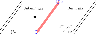
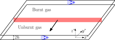
It is worth pointing out that the shear flow induces shear-enhanced diffusion (Taylor dispersion) in the flow -direction which can most strongly influence the burning speed of flames propagating in this direction [13, 14], such as in the case shown in Fig. 1(a). Since the enhancement of diffusion does not occur in the spanwise direction, the -direction in Fig. 1, the diffusion is effectively anisotropic. On account of the anisotropy, the flame structure and instabilities are expected to be significantly affected by the direction of flame propagation. This is particularly true when considering the direction of the planar flame whose stability is to be investigated; two important cases, shown in Fig. 1, are considered in this paper. These correspond respectively to flames propagating in the streamwise -direction, and the spanwise -direction. The second case, where the shear flow is parallel to the flame, is particularly relevant when addressing flame instabilities arising in a Taylor–Couette burner [15]; in this burner, the flame propagates parallel to the burner axis and the shear flow takes place in the azimuthal direction.
In addition to the anisotropy aspect aforementioned, Taylor dispersion also produces another intriguing effect related to the presence of a flow-dependent effective Lewis number in the streamwise direction, as reported in [14, 16]. Interestingly, the effective Lewis number approaches the inverse of the molecular Lewis number when the shear flow intensity becomes large, and this has surprising repercussions on the diffusive-thermal flame instabilities as reported in [10, 11, 12] for premixed flames and [17, 18] for diffusion flames. As we shall confirm below, similar repercussions of the effective Lewis number, coupled with the Darrieus–Landau instability, will appear in our study.
(a) Streamwise flame propagation
(b) Spanwise flame propagation
2 General formulation
In order to investigate the effect of a shear flow on the Darrieus–Landau instability, we shall adopt a plane Poiseuille flow in a Hele-Shaw channel, although another flow profile such as a Couette flow can also be used. The channel half-width is denoted by , and the velocity field and pressure gradient are given in a frame moving with the mean flow speed by
where is a unit vector in the -direction, the dynamic viscosity (assumed constant) and a modified pressure which includes the hydrostatic pressure and the term . We shall consider flame propagation in the narrow-channel limit , where is the laminar flame thickness. The chemistry is modelled by an irreversible reaction with an Arrhenius reaction rate , where is the density, is the pre-exponential factor, the mass fraction of the fuel (assuming to be the deficient species), the activation temperature and the temperature. The adiabatic flame temperature is defined by , where is the heat release parameter, the specific heat at constant pressure and is the amount of heat released per unit mass of fuel. Here and below, the subscripts and denote properties in the unburnt and burnt gas, respectively. For simplicity, we shall assume that the channel walls are adiabatic, and that and are constant, where is the thermal diffusivity.
Introduce the non-dimensional variables
where is the two-dimensional position vector, the laminar flame thickness, the laminar burning speed for , the Zeldovich number and Pr the Prandtl number. The non-dimensional governing equations in the low Mach-number approximation can then be written as
| (1) | |||
| (2) | |||
| (3) |
where , , is a unit vector in the direction of gravity (with ) and
Furthermore, is the Damköhler number, the flow Peclet number and the Rayleigh number. Note that is simply the ratio of the channel half-width to the laminar flame thickness.
3 Formulation for narrow channels
In the narrow-channel limit , the dependent variables are expanded as
Substituting these into Eqs. (1)-(3), and following the derivation presented in [19], two-dimensional equations can be obtained. These govern flame propagation in narrow adiabatic channels in a frame moving with the mean flow speed in the unburnt gas. Skipping algebraic details, the main results are as follows.
To leading order, the flow field corresponding to the imposed Poiseuille shear flow, is given by
At the first order, we obtain as in [20] and
where equations governing and can be obtained as solvability conditions of the second-order and third-order equations. The effective mass flux due to gas expansion can be defined as
Since the -component of is zero, we may regard as a two-dimensional vector field.
The equations satisfied by and are obtained, as mentioned above, from the solvability condition of the second-order equations. Dropping the subscript in , and , the final two-dimensional governing equations are found to be
| (4) | |||
| (5) | |||
| (6) | |||
| (7) |
with , and
By combining (4) and (6) and using (2), we obtain
| (8) |
The equation leads, when used with (5) and the relation , to the Poisson equation
| (9) |
for the pressure field. Equations (4)-(9) generalize similar equations used in the earlier study [9] to non-zero values of Pe. Notably, these equations clearly demonstrate the presence of anisotropic diffusion, and they will be used to study the stability of the planar flames in the two cases depicted in Fig. 1. Furthermore, as can be from from (8) the expansion rate of a fluid element is directly affected by the anisotropic heat conduction. It is also worth emphasising the presence in the modified Darcy equation (5) of an effective force induced by the imposed shear flow, given by . This term describes a novel aspect associated with the coupling between thermal expansion and Taylor dispersion, which has not been reported before and which has relevance well beyond combustion in areas involving transport phenomena. Furthermore, Eq. (5) implies that the vorticity is given by
| (10) |
This is a new result which indicates that curved flames in a Hele-Shaw channel always experience vorticity in the presence of Taylor dispersion, that is whenever , even in the absence of viscosity variations as assumed for simplicity in this paper. Equation (10) also implies that the vorticity field remains zero everywhere, except in (the preheat and reaction zones of) the flame where spatial density variations occur. As can be seen from the two-dimensional equations (4)-(7), the Peclet number enters only as , a behaviour that was originally pointed out by Zeldovich [21] in a related heat-transfer problem and obtained in other combustion studies such as in [22] in the case of narrow channels. Therefore whether the shear flow is in the positive or negative -directions is unimportant in the narrow-channel limit, under the simplifying constant-viscosity assumption adopted herein. This directional symmetry of the imposed flow is broken when next-order corrections to (4)-(7) are taken into account [20] or also when viscosity variations are taken into account. The reader may also refer to the recent study [23] on the flame hydrodynamic instabilities based on a different two-dimensional (Euler–Darcy) model taking into account viscosity variations.
4 Stability of a planar flame propagating in the streamwise direction
Consider a planar flame propagating steadily in the negative -direction as depicted in Fig. 1(a). Let be the (non-dimensional) flame burning speed, which is also its speed with respect to the mean flow. It is worth pointing out that the flame speed with respect to the walls is then given that is the non-dimensional mean flow speed (in the unburnt gas). Since Equations (4)-(9) are already written in a frame moving with the mean flow, it is sufficient in order to make the planar flame steady to shift the -coordinate by the amount . Therefore, effecting the transformation , the planar flame corresponds now to a steady solution depending only on . This steady solution is denoted using overbars and is characterised by a velocity and pressure field given by
and temperature and mass-fraction fields governed by
subject to the boundary conditions and .
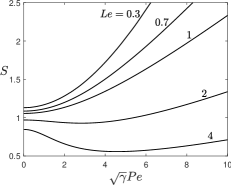
Note that the burning speed depends on the imposed shear flow whenever , due to shear-enhanced diffusion. In the asymptotic limit , as shown in [14, 20]. Here, we shall simply compute numerically for and , and the results are shown in Fig. 2 for selected values of Le.
To investigate the stability of the planar flame described above, we introduce
| (11) |
where the hat variables represent infinitesimal perturbations, is a real-valued spanwise wavenumber and is, in general, a complex-valued growth rate, which is to determined as an eigenvalue. The perturbations or hat variables are governed by linear equations which are given in the Appendix. These are solved numerically using COMSOL eigenvalue solver. All computations, here and below, are performed with the fixed values , and for selected values of Pe, Le and Ra. Before presenting the results, it is worth noting that the corresponding results for has been reported in the recent work [9] based on a two-dimensional model that can be obtained from ours by setting in (4)-(7).
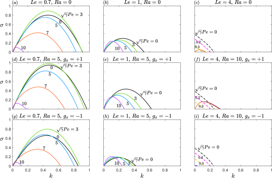
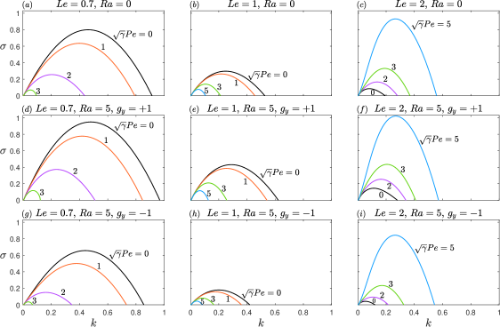
The results for streamwise propagation are summarised in Fig. 3. Shown is the real growth rate versus the spanwise wavenumber for selected values of Le, Ra and Pe. The left, middle and right columns correspond respectively to , and . The top, middle and bottom rows correspond respectively to (horizontal channels), with (gravity vector pointing towards burnt gas) and with (gravity vector pointing towards unburnt gas). In each subfigure, several curves are plotted for various values of Pe, which are indicated. The following main observations can be inferred from Fig. 3:
-
1.
For and , the effect of increasing Pe is to decrease the maximum growth rate and to reduce the range of unstable wavenumbers. This indicates an overall tendency of the shear flow to impede the Darrieus-Landau instability. Note that the slope of the curves for small values of increases with increasing Pe. This is associated with the growth rate being proportional to (for ), and being an increasing function of Pe as illustrated in Fig. 2.
-
2.
For , the Rayleigh–Taylor instability is seen to destabilize the flame when the gravity vector points towards to the burnt gas (middle row) and to stabilise otherwise (bottom row), as expected. It is worth noting that the effect of gravity on the dispersion curves becomes weak for large values of Pe; see the curves corresponding to .
-
3.
For , the growth rates are larger compared to those of the unit Lewis number cases, presumably due to such flames being prone to the cellular diffusive-thermal instability in addition to the Darrieus–Landau instability. Note that the effect of an increase in Pe is stabilising for sufficiently large values of Pe, but can be destabilising at smaller values as seen in the figure.
-
4.
For , in addition to the Darrieus–Landau instability, whose dispersion curves are plotted as solid lines, we also encounter the oscillatory diffusive-thermal instability, whose dispersion curves are plotted as dashed lines, indicating complex-valued growth rates. The latter instability is very sensitive to Pe, and disappear with slight increases in Pe, as found in [10].
5 Stability of a planar flame propagating in the spanwise direction
We consider now the case depicted in Fig. 1(b) where the unperturbed planar flame propagates steadily in the negative -direction with non-dimensional burning speed . Unlike the case of Fig. 1(a) addressed in the previous section, the planar flame and its burning speed are unaffected by the shear flow. The corresponding velocity and pressure field are given by
and the temperature and mass-fraction fields are governed by
subject to and . The value of here is independent of Pe and is equal to one in the asymptotic limit . For the finite value and adopted, takes the numerical values , , and for , and , respectively.
The stability of the planar flame is investigated now by writing
| (12) |
where the hat variables represent infinitesimal perturbations, the streamwise wavenumber and the growth rate. The linear system of equations governing the hat variables is given in the Appendix.
The results for spanwise propagation are summarised in Fig. 4. Shown is the real growth rate versus the streamwise wavenumber for selected values of Le, Ra and Pe. The left, middle and right columns correspond respectively to , and . The top, middle and bottom rows correspond respectively to (horizontal channels), with (gravity vector pointing towards burnt gas) and with (gravity vector pointing towards unburnt gas). In each subfigure, several curves are plotted for various values of Pe, which are indicated. The following main observations can be inferred from Fig. 4:
-
1.
For both and cases, the flame instability is impeded by increasing the shear strength. For , on the other hand, the instability is seen to be promoted by the shear flow.
-
2.
More generally, it is important to note that whereas the flame instability is promoted by a decrease in the value of Le for small or zero values of Pe, it is promoted by an increase in Le for larger values of Pe. This is an interesting result which has been also found and attributed to Taylor dispersion for constant density diffusive-thermally unstable flames [12].
6 Time-dependent numerical simulations
Time-dependent computations using Eqs. (5)-(7) and (9) and an initial condition corresponding to a planar flame solution (to which small amplitude random perturbations are added) are performed using COMSOL Multiphysics, following the methodology described in [11, 20]. A nonuniform grid with typically 300 000 triangular elements is chosen with local refinement around the reaction zone. In the case of streamwise propagation, a frame moving in the negative -direction with the flame is adopted whose speed with respect to the unburnt gas is taken to be equal to the total instantaneous burning rate per unit transverse domain size . With respect to the channel walls, the adopted frame moves with the speed , where is the non-dimensional mean flow speed of the unburnt gas, which can take both positive and negative values. In the case of spanwise propagation, the adopted frame moves in the negative -direction with the speed and in the negative -direction with the speed . Note that the governing Eqs. (5)-(7) and (9), are already written in a frame moving with the mean flow in the -direction and are independent of the sign of Pe, as noted at the end of section 3. The solutions obtained and described below are thus valid both for positive and negative values of the mean flow speed . The boundary conditions in the frame adopted correspond to far ahead of the flame in the unburnt gas, and to far in the burnt gas. Periodic boundary conditions are imposed in the transverse direction. The domain extent in the direction of propagation is taken equal to and in the transverse direction.
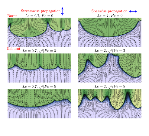
Illustrative results for six cases are presented in Fig. 5. Shown are instantaneous temperature fields and streamlines in the frame moving with the flame adopted at selected times long after the instability has developed. The double-headed arrow is in the direction of the imposed shear flow and indicates the equivalence of two opposite parallel directions of the flow. As emphasised at the end of section 3, the later equivalence ceases to hold when the constant-viscosity assumption is relaxed (see, for instance [23]) or in wider channels (see, e.g., [20]).
Several important observations can be inferred from the figure (and from examination of the animations provided as supplementary material). For streamwise propagation (the subfigures in the left column), it is seen that an increase in Pe tends to flatten and thicken the flame and weaken its wrinkles. As for spanwise propagation (the subfigures in the right column), the opposite tendency is observed. It is worth noting that the streamlines are deflected in an unusual fashion for higher values of Pe, with the appearance of a stagnation point within the flame preheat zone accompanied by the presence of counter-rotating vortices; see middle and bottom subfigures in right column and compare with top subfigure. The presence of such vortices, and more generally the presence of vorticity within the flame and nowhere else around it, can be explained by the remarks following Eq. (10). Finally, note the unusual presence of structures with pointed leading edges close to the counter-rotating vortices. The reader is referred to the supplementary materials for a better appreciation of the full time evolution of the unstable flames.
7 Conclusions
In this paper, we have investigated the effect of a shear flow on the Darrieus–Landau instability in a Hele-Shaw channel. It is found that a strong shear flow tends to suppress the flame instability in the case of streamwise flame propagation. On the other hand, for flame propagation in the spanwise direction, the shear flow is found to have a destabilizing effect in mixtures and a stabilizing effect in mixtures. Furthermore, for unstable flames propagating in the streamwise direction, the flow tends to mitigate flame wrinkling, whereas the opposite tendency is encountered for flames propagating in the spanwise direction. An original result revealed by this study, is that curved flames in a Hele-Shaw channel always experience vorticity in the presence of Taylor dispersion, that is whenever , even in the absence of gravity and viscosity variations.
One of the interesting findings correspond to the peculiar flame shapes encountered including cusps pointing towards to the unburnt gas and counter-rotating vortices in the case of spanwise flame propagation. This finding should stimulate future experimental investigations to observe such patterns, especially within the Taylor–Couette burner configuration [15], where the direction of the shear flow is transverse to that of flame propagation. Finally, the analysis of the effect of Taylor dispersion on the flame hydrodynamic instabilities, explored here for a steady imposed flow, is worth extending to other shear flows; these include oscillatory flows [24] and spatio-temporal periodic flows [25]. Such extension would complement recent theoretical and experimental findings on flame instabilities in such oscillatory flows [26].
Declaration of competing interest
The authors declare that they have no known competing financial interests or personal relationships that could have appeared to influence the work reported in this paper.
Acknowledgments
This work was supported by the UK EPSRC through grant EP/V004840/1.
Supplementary material
Animated time evolution of numerical simulations are included as video files.
Appendix
In this appendix, we write down the linear system of equation corresponding to the linear stability analysis of the planar premixed flames propagating either in the streamwise direction as in Fig. 1(a), or in the spanwise direction as in Fig. 1(b). The system is an eigen-boundary value problem for the perturbations , , and introduced in Eqs. (11) and (12). For convenience, we also use the auxiliary variables , , , and , which are expressible in terms of , , and . For example, and
For the case of streamwise propagation, we obtain the system of equations
subject to as . Here and below prime denotes differentiation of a function with respect to its argument. It can be checked that these equations reduce to those reported in [9] when and .
For the case of spanwise propagation, we obtain the system of equations
subject to as .
References
- [1] F. Veiga-López, M. Kuznetsov, D. Martínez-Ruiz, E. Fernández-Tarrazo, J. Grune, M. Sánchez-Sanz, Unexpected propagation of ultra-lean hydrogen flames in narrow gaps, Phys. Rev. Lett. 124 (17) (2020) 174501.
- [2] G. Gu, J. Huang, W. Han, C. Wang, Propagation of hydrogen–oxygen flames in Hele-Shaw cells, Int. J. Hydrog. Energy 46 (21) (2021) 12009–12015.
- [3] J. Yanez, M. Kuznetsov, F. Veiga-López, On the velocity, size, and temperature of gaseous dendritic flames, Phys. Fluids 34 (11).
- [4] E. Al Sarraf, C. Almarcha, J. Quinard, B. Radisson, B. Denet, P. Garcia-Ybarra, Darrieus–Landau instability and markstein numbers of premixed flames in a Hele-Shaw cell, Proc. Combust. Inst. 37 (2) (2019) 1783–1789.
- [5] F. Veiga-López, D. Martínez-Ruiz, E. Fernández-Tarrazo, M. Sánchez-Sanz, Experimental analysis of oscillatory premixed flames in a Hele-Shaw cell propagating towards a closed end, Combust. Flame 201 (2019) 1–11.
- [6] M. Tayyab, B. Radisson, C. Almarcha, B. Denet, P. Boivin, Experimental and numerical lattice-Boltzmann investigation of the Darrieus–Landau instability, Combust. Flame 221 (2020) 103–109.
- [7] Y. Han, M. Modestov, D. M. Valiev, Effect of momentum and heat losses on the hydrodynamic instability of a premixed equidiffusive flame in a Hele-Shaw cell, Phys. Fluids 33 (10).
- [8] A. Domínguez-González, D. Martínez-Ruiz, M. Sánchez-Sanz, Stable circular and double-cell lean hydrogen-air premixed flames in quasi two-dimensional channels, Proc. Combust. Inst. 39 (2) (2023) 1731–1741.
- [9] D. Fernández-Galisteo, V. N. Kurdyumov, Impact of the gravity field on stability of premixed flames propagating between two closely spaced parallel plates, Proc. Combust. Inst. 37 (2) (2019) 1937–1943.
- [10] J. Daou, Effect of Taylor dispersion on the thermo-diffusive instabilities of flames in a Hele-Shaw burner, Combust. Theory Model. 25 (4) (2021) 765–783.
- [11] J. Daou, A. Kelly, J. Landel, Flame stability under flow-induced anisotropic diffusion and heat loss, Combust. Flame 248 (2023) 112588.
- [12] J. Daou, P. Rajamanickam, Diffusive-thermal instabilities of a planar premixed flame aligned with a shear flow, Combust. Theory Model. 28 (1) (2024) 20–35.
- [13] P. Pearce, J. Daou, Taylor dispersion and thermal expansion effects on flame propagation in a narrow channel, J. Fluid Mech. 754 (2014) 161–183.
- [14] J. Daou, P. Pearce, F. Al-Malki, Taylor dispersion in premixed combustion: Questions from turbulent combustion answered for laminar flames, Phys. Rev. Fluids 3 (2) (2018) 023201.
- [15] V. Vaezi, R. C. Aldredge, Laminar-flame instabilities in a Taylor–Couette combustor, Combust. Flame 121 (1-2) (2000) 356–366.
- [16] A. Liñán, P. Rajamanickam, A. D. Weiss, A. L. Sánchez, Taylor-diffusion-controlled combustion in ducts, Combust. Theory Model. 24 (6) (2020) 1054–1069.
- [17] P. Rajamanickam, A. Kelly, J. Daou, Stability of diffusion flames under shear flow: Taylor dispersion and the formation of flame streets, Combust. Flame 257 (2023) 113003.
- [18] A. Kelly, P. Rajamanickam, J. Daou, J. Landel, Influence of heat loss on the stability of diffusion flames in a narrow-channel shear flow, Combust. Sci. Technol.
- [19] P. Rajamanickam, A. D. Weiss, Effects of thermal expansion on Taylor dispersion-controlled diffusion flames, Combust. Theory Model. 26 (1) (2022) 50–66.
- [20] P. Rajamanickam, J. Daou, A thick reaction zone model for premixed flames in two-dimensional channels, Combust. Theory Model. 27 (4) (2023) 487–507.
- [21] Y. B. Zeldovich, The asymptotic law of heat transfer at small velocities in the finite domain problem, Zh. Eksp. Teoret. Fiz 7 (12) (1937) 1466–1468.
- [22] J. Daou, M. Matalon, Flame propagation in poiseuille flow under adiabatic conditions, Combust. Flame 124 (3) (2001) 337–349.
- [23] T. Miroshnichenko, V. Gubernov, S. Minaev, Hydrodynamic instability of premixed flame propagating in narrow planar channel in the presence of gas flow, Combust. Theory Model. 24 (2) (2020) 362–375.
- [24] E. Watson, Diffusion in oscillatory pipe flow, J. Fluid Mech. 133 (1983) 233–244.
- [25] P. Rajamanickam, J. Daou, Effective Lewis number and burning speed for flames propagating in small-scale spatio-temporal periodic flows, Combust. Flame 258 (2023) 113077.
- [26] B. Radisson, B. Denet, C. Almarcha, Forcing of a flame by a periodic flow in a Hele-Shaw burner, Phys. Rev. Fluids 7 (5) (2022) 053201.