Image-Conditional Diffusion Transformer for Underwater Image Enhancement

Abstract

Underwater image enhancement (UIE) has attracted much attention owing to its importance for underwater operation and marine engineering. Motivated by the recent advance in generative models, we propose a novel UIE method based on image-conditional diffusion transformer (ICDT). Our method takes the degraded underwater image as the conditional input and converts it into latent space where ICDT is applied. ICDT replaces the conventional U-Net backbone in a denoising diffusion probabilistic model (DDPM) with a transformer, and thus inherits favorable properties such as scalability from transformers. Furthermore, we train ICDT with a hybrid loss function involving variances to achieve better log-likelihoods, which meanwhile significantly accelerates the sampling process. We experimentally assess the scalability of ICDTs and compare with prior works in UIE on the Underwater ImageNet dataset. Besides good scaling properties, our largest model, ICDT-XL/2, outperforms all comparison methods, achieving state-of-the-art (SOTA) quality of image enhancement.

I Introduction

Underwater imaging has been widely used in underwater archaeology, underwater robotics, marine detection, and other fields[1, 2, 3]. However, wavelength- and distance-dependent light attenuation and scattering cause the problem of low contrast and color deviation in underwater images. These degraded images not only lead to unsatisfactory visual experience for humans but also affect the performance in computer vision tasks like object detection, image classification, and semantic segmentation.

To enhance the quality of underwater images, scholars have proposed a series of effective measures, promoting the development of underwater image enhancement (UIE). Conventional UIE methods[4, 5, 6, 7, 8, 9] (e.g., white balance[4, 5] and histogram equalization[6]) depend on assumptions or a priori knowledge, models, or design guidelines to enhance underwater images. Although conventional methods are easy to execute, they are not adaptable to different water environment and lighting conditions.

The rapid development of deep learning brings new insights and tools for UIE. By leveraging large-scale underwater image datasets to learn the patterns and features, deep-learning-based UIE methods can achieve intelligent, automated, and end-to-end underwater image enhancement. Deep-learning-based UIE methods are typically divided into two primary categories: 1) convolutional neural network (CNN)-based[10, 11, 12, 13, 14, 15] and 2) generative adversarial network (GAN)-based[16, 17, 18, 19, 20, 21]. The CNN-based UIE methods train deep CNNs to learn the mapping relationship from the degraded image to the high-quality reference image[10], which is robust to different underwater scenes. The GAN-based UIE can also accomplish the conversion from the degraded underwater image to the corresponding ground truth image and achieve good performance[16]. However, GANs often suffer from unstable training process and mode collapse. Therefore, it is necessary to develop more stable and diversified methods to further improve the effect and quality of UIE.

Denoising diffusion probabilistic models (DDPM) have begun to attract extensive attention for its good convergence properties and relatively stable training process. DDPMs have emerged as a new state-of-the-art (SOTA) baseline in the field of image generation[22, 23]. As scholars continue to explore diffusion models, their potential for image-to-image generation is continually developed[24]. In image restoration, image coloring, and image super-resolution tasks, diffusion model-based approaches have produced superior results than GAN models[22, 23, 24]. Although DDPMs can yield excellent results, an acknowledged challenge of DDPMs is the long inference time, which leads to poor real-time performance.

In this article, a generative approach for UIE based on conditional DDPM is proposed, which uses the degraded image as the conditional input. As for the model architecture, the conventional U-Net[25] backbone in a diffusion model is replaced with a transformer, which we call image-conditional diffusion transformer (ICDT). Diffusion transformer adheres to many good practices of vision transformers (ViT)[26], perhaps one of the most important factors is the excellent scalability properties compared to traditional convolutional networks. Moreover, we incorporate learnt variances into DDPMs with reference to[27], allowing DDPMs to sample in much fewer steps without sacrificing sample quality.

The main contributions of this paper are summarized as follows:

1. We use a transformer as the backbone of the DDPM instead of the U-Net, which retains favorable properties like scalability from ViTs. The scaling performance is explored through experiments, where we find a strong correlation between the sample quality and network complexity (measured by FLOPs). Images of different quality generated by models with different complexity can meet the requirements for various downstream tasks (e.g., object detection, image classification, and semantic segmentation) and scenes, achieving a reasonable match between image-quality requirement and computing power. Furthermore, our most computational intensive model achieves a SOTA result on the standard benchmark dataset (Underwater ImageNet).

2. The degraded image is used as the extra conditional input to the DDPM for UIE. It is converted to latent via a VAE along with the corresponding reference image. The generated conditional latent and noised latent are then concatenated channel-wise. The transformer is applied to the latent space, constituting a computational-efficient hybrid architecture referred to as ICDT. The proposed ICDT has the potential to become a universal framework for image-to-image generation tasks such as image restoration, image enhancement, image translation, image coloring, and image super-resolution.

3. A hybrid loss function which provides learning signal for variances is employed in training of ICDT to achieve better log-likelihoods. Furthermore, incorporating learnt variances into DDPMs can considerably speed up sampling with a negligible change in sample quality, which is important for deployment in practical applications.

The remainder of the article is organized as follows. In Section II, the related work is reviewed. Section III describes the proposed ICDT in detail. In Section IV, the experimental setup is presented. Extensive experiments are conducted to explore the scaling properties and demonstrate the effectiveness and performance of the ICDT method for UIE in Section V. Finally, Section VI concludes this article.

II Related Work

II-A Conventional UIE Method

Conventional UIE methods depend on assumptions or a priori knowledge, models, or design rules to enhance underwater images. These methods are based on physical models and utilize image degradation priors to inversely solve degradation models. Drews et al.[7] introduced a UIE method using underwater dark channel prior (DCP), which utilizes the statistical prior of images obtained in outdoor natural scenes and applies it only in the blue and green channels to improve enhancement quality. Li et al.[6] minimized the information loss of the enhanced underwater images to obtain the transmission map and improved the brightness and contrast of underwater images based on natural image histogram distribution prior. Wang et al.[8] proposed the maximum attenuation identification method for UIE based on a simplified underwater light propagation model. Ancuti et al.[4] combined the Laplacian pyramid and white balance to produce two enhanced results, which were then fused via weight mapping. Peng et al.[9] generalized the common DCP method to image restoration. They estimated scene transmission through calculating the difference between the ambient light and the observed intensity. In addition, they incorporated adaptive color correction into the image formation model to remove color casts and restore contrast.

Although these methods have specific theoretical support, they may still suffer from under-enhancement or over-enhancement under challenging water environment and lighting condition. One reason is that the underwater environment is complex and changeable, and physical parameters are difficult to get; the other reason is that the underwater image degradation model is different from that on land and difficult to establish.

II-B Deep-Learning-Based UIE Method

With tremendous progress of deep learning in computer vision, deep-learning-based methods have emerged as the baseline for UIE tasks in recent years. The deep learning-based methods trained with different types of underwater images can break through the limitation of conventional methods. Deep-learning-based methods mainly consist of two categories: CNN-based and GAN-based.

CNN extracts hierarchical high-level image features based on convolution and pooling, enabling automatic learning of effective features in underwater images. Among them, Sun et al.[11] proposed a deep pixel-to-pixel network with an encoder–decoder framework for UIE. It uses convolution layers as encoder for noise filtering, while uses deconvolution layers as decoder for detail recovery and image refinement, achieving self-adaptive data-driven image enhancement without considering the physical environment. Li et al.[12] proposed a gated fusion network called Water-Net for UIE, which fuses the input images into the enhanced result according to the predicted confidence maps. The predicted confidence maps learnt by Water-Net determine the most significant features of input images left in the enhanced result. Li et al.[13] presented a light-weight CNN (UWCNN) based on underwater scene prior, which is trained with the corresponding data to accommodate various underwater scenes. Naik et al.[14] proposed a shallow neural network architecture (Shallow-UWnet) for UIE, which has fewer parameters than the state-of-art models while preserving good performance. Li et al.[15] utilized CNN coupled with attention mechanism to extract the most discriminative features from multiple color spaces and adaptively integrate and highlight them, which improves the visual quality of underwater images effectively. The above methods benefit from the efficacy and generalization ability of CNN, which brings considerable improvement to UIE. However, the finite receptive field restricts CNN-based methods from modeling long-range pixel dependence, and the fixed weight of CNN also affects its adaptation to different input contents.

GAN[28, 29, 30] is a deep-learning-based generative model. In recent years, GAN has been extensively applied in UIE to improve the usability and visual quality of underwater images. For example, Li et al.[17] proposed WaterGAN to enable real-time color correction for underwater images, which can produce realistic underwater images from in-air image and depth map pairs in an unsupervised manner, and coarsely estimate the depth of underwater scenes. Islam et al.[18] proposed FUnIEGAN for real-time UIE based on conditional GAN. A comprehensive objective function which associates image content, global similarity, and local texture and style is introduced to guide adversarial training, leading to better perceptual image quality for both paired and unpaired training. Liu et al.[19] presented MLFcGAN which enhances the color and contrast of underwater images by fusing multilevel features. MLFcGAN augments local features in each level with global features, improving the learning speed and the performance in color correction and detail preservation of the network. Han et al.[20] introduced a light-weight encoder-decoder architecture (UIENet) to enhance underwater images from visual sensors. UIENet is further involved into a generative adversarial network (UIEGAN) model against a supervised discriminator to improve its correction capability for the photorealistic images with more global information and local details. Cong et al.[21] proposed a physical model-guided GAN for UIE to promote the reality and visual aesthetics of the enhanced images. However, the training processes of these GAN-based UIE methods are often divergent or unstable, and the generated images often suffer from uncertainty or a lack of diversity. Therefore, it is difficult to ensure the accuracy and consistency of generated results.

Although deep learning-based methods have greatly promoted the development of UIE over recent years, there are still some obstacles to overcome.

II-C Denoising Diffusion Probabilistic Models

DDPMs[31] have made great success in the field of image generation[32, 33, 34, 35, 36], which outperforms GANs, the previous SOTA method, in many tasks. DDPM is a class of simplified diffusion model which applies variational inference for modeling and reparameterization trick for sampling. In general, the DDPM includes two processes: the forward noising process (i.e., diffusion process) and the reverse denoising process. The forward noising process gradually injects Gaussian noise to the clean image, making it more and more random and blurry until it approximates an isotropic Gaussian distribution. The reverse denoising process reconstructs the original image from a Gaussian-distributed noisy image by gradually removing noise. The reverse process trains a neural network to estimate the conditional probability distribution at each step, more specifically, the data distribution of the previous step given the current data. DDPM has demonstrated the advantage of more stable training process and higher quality and diversity of synthesis.

Recent advances of DDPMs have been largely due to reformulating DDPMs to estimate noise rather than pixels[31], utilizing cascaded DDPM pipelines in which low-resolution base diffusion models are trained in concurrence with upsamplers[32, 37], and improved sampling techniques[31, 38, 39]. For example, Nicholas et al.[27] introduced improved DDPMs (IDDPM), which can obtain better log-likelihood and high-quality samples. Saharia et al.[37] presented a class-conditional diffusion model named cascaded diffusion models (CDM) for high-fidelity image generation, which utilizes category labels as input conditions to produce images of the corresponding category. Saharia et al.[23] also proposed super-resolution via repeated refinement (SR3). SR3 is a conditional DDPM that uses a low-resolution image as input condition and generates the corresponding high-resolution image through an iterative stochastic denoising process.

Currently, DDPMs have been applied to image reconstruction tasks[35, 40, 41]. Kawar et al.[42] introduced denoising diffusion restoration models (DDRMs) which utilizes a pre-trained denoising diffusion generative model to solve a linear inverse problem since image restoration can usually be represented as a linear inverse problem. DDRM denoises a sample to the desired output gradually and stochastically, conditioned on the inverse problem and measurements. In this way a variational inference objective is employed to learn the posterior distribution, from which images are produced efficiently. Lu et al.[43] first presented a DDPM-based UIE method (UW-DDPM), which uses two U-Net networks for image distribution transformation and image denoising, effectively enhancing the underwater images. However, that work does not address the issue of slow sampling speed of DDPMs and its application scenarios are substantially limited. Lu et al.[44] further proposed SU-DDPM for UIE, which reduces the sampling step and changes the initial sampling distribution to accelerate the sampling inference process and achieve real-time enhancement. Additionally, SU-DDPM combines the reference image with the degraded image in the diffusion process, effectively solving the issue of color deviation and improving the quality of underwater images. Convolutional U-Nets[25] are presently the prevailing choice for backbone architecture of DDPMs. Concurrent work[45] introduced a new, efficient DDPM architecture which is based on attention mechanisms. Inspired by these diffusion models mentioned above, we propose ICDT to enhance underwater images.

III Image-Conditional Diffusion Transformer

Conditional diffusion models take supplemental information as input. For UIE task, we use degraded image as the extra conditional input. Additionally, a few simple modifications are done following[27] to make DDPMs achieve better log-likelihoods and sample much faster without sacrificing sample quality.

III-A Image-Conditional Denoising Diffusion Probabilistic Models

DDPMs[31] are a kind of generative models which progressively transforms a Gaussian noise distribution into the distribution of data on which the model is trained. The forward noising process is a Markov process which gradually corrupts the data ${{\bf{x}}_{0}}\sim q({{\bf{x}}_{0}})$ by injecting Gaussian noise with variance $\beta_{t}\in(0,1)$ at time $t$

$$q({\bf{x}}_{1:T}|{\bf{x}}_{0}) =\prod\limits_{t=1}^{T}q({\bf{x}}_{t}|{\bf{x}}_{t-1}),$$ (1)

$$q({{\bf{x}}_{t}}|{{\bf{x}}_{t-1}}) ={\cal N}({{\bf{x}}_{t}};\sqrt{1-{\beta_{t}}}{{\bf{x}}_{t-1}},{\beta_{t}}{\bf{I}}).$$ (2)

Given sufficiently large $T$ and an appropriate schedule of $\beta_{t}$, ${\bf{x}}_{T}$ approximately obeys an isotropic Gaussian distribution. Thus, if the reverse distribution $q({\bf{x}}_{t-1}|{\bf{x}}_{t})$ is known, we can start from ${{\bf{x}}_{T}}\sim{\cal N}(0,{\bf{I}})$ and run the reverse process to obtain a sample from $q({{\bf{x}}_{0}})$.

During training we sample a data pair $({\bf{x}}_{0},{\bf{\tilde{x}}})$ where ${\bf{\tilde{x}}}$ is a degraded image and ${\bf{x}}_{0}$ is the corresponding ground truth image. Conditional diffusion models use a neural network to learn the reverse process defined by the conditional joint distribution

$$p_{\theta}({\bf{x}}_{0:T}|{\bf{\tilde{x}}}) =p({\bf{x}}_{T})\prod\limits_{t=1}^{T}{p_{\theta}({\bf{x}}_{t-1}|{\bf{x}}_{t},{\bf{\tilde{x}}})},$$ (3)

$$p_{\theta}({\bf{x}}_{t-1}|{\bf{x}}_{t},{\bf{\tilde{x}}}) ={\cal N}({\bf{x}}_{t-1};{\boldsymbol{\mu}}_{\theta}({\bf{x}}_{t},{\bf{\tilde{x}}},t),{\bf{\Sigma}}_{\theta}({\bf{x}}_{t},{\bf{\tilde{x}}},t)),$$ (4)

so that the sampled image in the diffusion process has high fidelity to the data distribution conditioned on ${\bf{\tilde{x}}}$ (cf. Fig. 1).

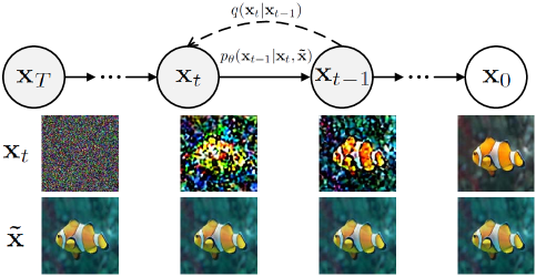
Figure 1: The forward noising process (dashed line) and the reverse denoising process (solid line) of an image-conditional DDPM.

Here ${\boldsymbol{\mu}}_{\theta}({\bf{x}}_{t},{\bf{\tilde{x}}},t)$ and ${\bf{\Sigma}}_{\theta}({\bf{x}}_{t},{\bf{\tilde{x}}},t)$, the statistics of $p_{\theta}$, are estimated by the neural network where ${\bf{\tilde{x}}}$ is provided as input.

The loss function which the model is trained with is a variational lower bound (VLB)[46] of the negative log likelihood $\mathbb{E}_{q({\bf{x}}_{0})}[-\log p_{\theta}({\bf{x}}_{0})]\leq L_{\rm{vlb}}$, and the VLB can be written as[31, 32]

$${L_{\rm{vlb}}} =\mathbb{E}_{q}\left[{\underbrace{{D_{{\rm{KL}}}}(q({{\bf{x}}_{T}}|{{\bf{x}}_{0}})||p({{\bf{x}}_{T}}))}_{{L_{T}}}\underbrace{-\log{p_{\theta}}({{\bf{x}}_{0}}|{{\bf{x}}_{1}},{\bf{\tilde{x}}})}_{{L_{0}}}}\right.$$

$$\hskip 11.00008pt\left.{+\sum\limits_{t>1}{\underbrace{{D_{{\rm{KL}}}}(q({{\bf{x}}_{t-1}}|{{\bf{x}}_{t}},{{\bf{x}}_{0}})||{p_{\theta}}({{\bf{x}}_{t-1}}|{{\bf{x}}_{t}},{\bf{\tilde{x}}}))}_{{L_{t-1}}}}}\right].$$ (5)

The loss can be efficiently optimized through stochastic gradient descent over uniformly sampled $L_{t-1}$ terms[31], taking into account that we can sample intermediate ${\bf{x}}_{t}$ from an arbitrary step of the diffusion process with the marginal

$$q({{\bf{x}}_{t}}{\rm{|}}{{\bf{x}}_{0}})={\cal N}({{\bf{x}}_{t}};\sqrt{{{\bar{\alpha}}_{t}}}{{\bf{x}}_{0}},(1-{\bar{\alpha}_{t}}){\bf{I}}),$$ (6)

or

$${{\bf{x}}_{t}}=\sqrt{{{\bar{\alpha}}_{t}}}{{\bf{x}}_{0}}+\sqrt{1-{{\bar{\alpha}}_{t}}}{{\boldsymbol{\epsilon}}_{t}},$$ (7)

where ${\alpha_{t}}=1-{\beta_{t}}$, ${\bar{\alpha}_{t}}=\prod\nolimits_{i=0}^{t}{{\alpha_{i}}}$, and ${\boldsymbol{\epsilon}}_{t}\sim{\cal N}({\bf{0}},{\bf{I}})$. The $L_{t-1}$ term in (III-A) is a KL divergence between two Gaussian distributions, $p_{\theta}({\bf{x}}_{t-1}|{\bf{x}}_{t},{\bf{\tilde{x}}})$ from (4) and $q({{\bf{x}}_{t-1}}|{{\bf{x}}_{t}},{{\bf{x}}_{0}})$. The latter is the generative process posterior, which can be calculated using Bayes theorem

$$q({{\bf{x}}_{t-1}}{\rm{|}}{{\bf{x}}_{t}},{{\bf{x}}_{0}})={\cal N}({{\bf{x}}_{t-1}};{{\boldsymbol{\tilde{\mu}}}_{t}}({{\bf{x}}_{t}},{{\bf{x}}_{0}}),{\tilde{\beta}_{t}}{\bf{I}})$$ (8)

where the parameters of the distribution are defined as

$${{\boldsymbol{\tilde{\mu}}}_{t}}({{\bf{x}}_{t}},{{\bf{x}}_{0}}) =\frac{{\sqrt{{{\bar{\alpha}}_{t-1}}}{\beta_{t}}}}{{1-{{\bar{\alpha}}_{t}}}}{{\bf{x}}_{0}}+\frac{{\sqrt{{\alpha_{t}}}(1-{{\bar{\alpha}}_{t-1}})}}{{1-{{\bar{\alpha}}_{t}}}}{{\bf{x}}_{t}},$$ (9)

$${\tilde{\beta}_{t}} =\frac{{(1-{{\bar{\alpha}}_{t-1}})}}{{(1-{{\bar{\alpha}}_{t}})}}{\beta_{t}}.$$ (10)

Since both $q$ and $p_{\theta}$ are Gaussian, we evaluate the KL divergence with the mean and covariance of them. The mean ${\boldsymbol{\mu}}_{\theta}({\bf{x}}_{t},{\bf{\tilde{x}}},t)$ can be parameterized in many different ways. For example, we could predict ${\boldsymbol{\mu}}_{\theta}({\bf{x}}_{t},{\bf{\tilde{x}}},t)$ directly or predict ${\bf{x}}_{0}$ and use it in (9) to get ${\boldsymbol{\mu}}_{\theta}({\bf{x}}_{t},{\bf{\tilde{x}}},t)$. Alternatively, one can predict the noise ${\boldsymbol{\epsilon}}_{t}$ and incorporate (7) into (9) to derive[15]

$${\boldsymbol{\mu}}_{\theta}({\bf{x}}_{t},{\bf{\tilde{x}}},t)=\frac{1}{{\sqrt{{\alpha_{t}}}}}\left({{{\bf{x}}_{t}}-\frac{{{\beta_{t}}}}{{\sqrt{1-{{\bar{\alpha}}_{t}}}}}{{\boldsymbol{\epsilon}}_{\theta}}({\bf{x}}_{t},{\bf{\tilde{x}}},t)}\right).$$ (11)

For image-based conditioning, ${\bf{x}}_{t}$ and ${\bf{\tilde{x}}}$ are channel-wise concatenated as the input of the neural network. In this setting the neural network is trained to predict ${\boldsymbol{\epsilon}}_{t}$ by optimizing the mean-squared error objective

$${L_{{\rm{simple}}}}={\mathbb{E}_{{{\bf{x}}_{0}},t,{\boldsymbol{\epsilon}}_{t}}}[||{{\boldsymbol{\epsilon}}_{t}}-{{\boldsymbol{\epsilon}}_{\theta}}({{\bf{x}}_{t}},{\bf{\tilde{x}}},t)|{|^{2}}].$$ (12)

This simplified objective can be viewed as a re-weighted version of $L_{\rm{vlb}}$, which omits the terms involving ${\bf{\Sigma}}_{\theta}$.

To improve the log-likelihood of ${\bf{x}}_{0}$, a better choice of ${\bf{\Sigma}}_{\theta}({\bf{x}}_{t},{\bf{\tilde{x}}},t)$ is needed. Since $L_{{\rm{simple}}}$ provides no learning guidance for ${\bf{\Sigma}}_{\theta}({\bf{x}}_{t},{\bf{\tilde{x}}},t)$, a hybrid objective is introduced[27]

$${L_{{\rm{hybrid}}}}={L_{{\rm{simple}}}}+\lambda{L_{{\rm{vlb}}}},$$ (13)

where ${\bf{\Sigma}}_{\theta}({\bf{x}}_{t},{\bf{\tilde{x}}},t)$ is learnt via $L_{{\rm{vlb}}}$ while $L_{{\rm{simple}}}$ remains the main source of impact on ${\boldsymbol{\mu}}_{\theta}({\bf{x}}_{t},{\bf{\tilde{x}}},t)$ with small $\lambda$ (e.g., $\lambda=0.001$) to keep $L_{{\rm{vlb}}}$ from overwhelming $L_{{\rm{simple}}}$.

Additionally, it has been shown that incorporating learnt variances into DDPMs allows sampling with much fewer diffusion steps than training with a negligible change in sample quality[27]. During sampling we only need a sub-sequence of the complete $\{1,...,T\}$ timestep indices, e.g. a sub-sequence with uniformly spaced integers between $1$ and $T$. While DDPM[31] needs hundreds of sampling steps to generate high-quality images, we can achieve almost the same quality with an order of magnitude fewer sampling steps, thus accelerating sampling for deployment in practical applications.

III-B Architecture of Image-Conditional Diffusion Transformer

The architecture of the proposed ICDT is based on diffusion transformer. Since the focus of diffusion transformer is on learning spatial representations of images, it operates on sequences of patches like vision transformer (ViT)[26]. Moreover, diffusion transformer retains many good practices of ViTs. Fig. 2 illustrates an overview of the complete ICDT architecture and we will describe its forward pass in detail as follows.

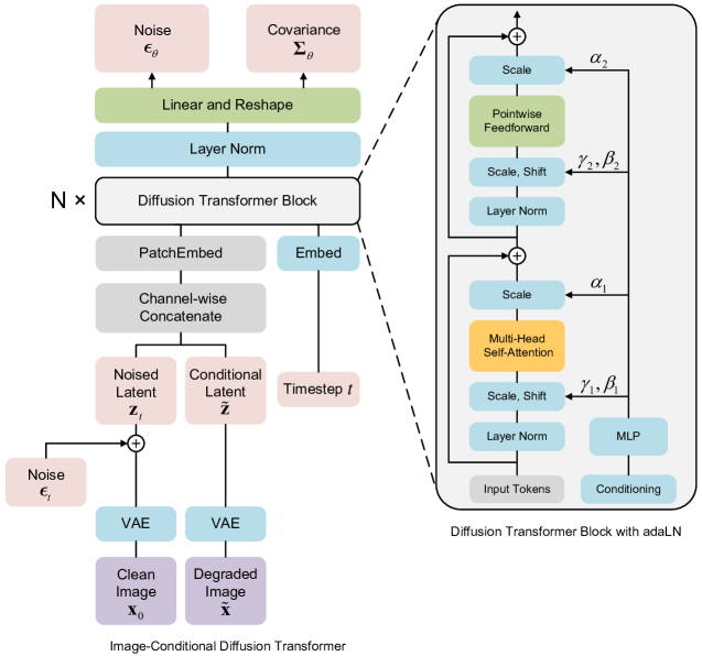
Figure 2: The ICDT architecture. Left: We train ICDT models in latent space. The converted latent is divided into patches and subsequently processed by $N$ diffusion transformer blocks. Right: Details of the diffusion transformer blocks which incorporate conditioning through adaptive layer norm.

It is computationally prohibitive to train diffusion models directly in pixel space, especially for large-size images. Latent diffusion models (LDMs)[35] address this problem through a two-stage approach: (1) train an autoencoder which compresses images into small spatial representations via a learned encoder ${\bf{z}}=E(\bf{x})$; (2) train a diffusion model for representations $\bf{z}$ rather than for images $\bf{x}$ ($E$ is fixed). Generated images can be obtained by decoding a sample $\bf{z}$ from the diffusion model to an image via the learned decoder ${\bf{x}}=D(\bf{z})$. LDMs achieve comparable performance while occupying much fewer FLOPs than pixel space diffusion models, which makes them an attractive option for architecture design. In consideration of computational efficiency, we employ diffusion transformers to latent space, which renders the image generation pipeline a hybrid architecture. Specifically, in the hybrid model we apply pre-trained variational autoencoders (VAEs) and transformer-based DDPMs.

For image-conditional diffusion models, the conditional image (degraded image in this setting) $\bf{\tilde{x}}$ is provided as input. As shown in Fig. 2, the input images ${\bf{x}}_{0}$ and $\bf{\tilde{x}}$ pass through the VAEs, converted to latents ${\bf{z}}_{0}$ and $\bf{\tilde{z}}$ with shape $I\times I\times C$. Then, the noised latent ${\bf{z}}_{t}$ is obtained according to (7). We concatenate ${\bf{z}}_{t}$ and $\bf{\tilde{z}}$ channel-wise, doubling the input channel dimension for diffusion transformer.

The first layer of ICDT is “patchembed”, which implements patchifying and embedding. Patchifying reshapes the spatial representations ${\bf{z}}_{t}$ and $\bf{\tilde{z}}$ into a sequence of $T$ flattened 2D patches. The number of patches $T$ depends on the patch size hyperparameter $p$, more specifically, $T=(I/p)^{2}$. Doubling $P$ will quarter $T$, and thus quarter total transformer FLOPs at least. Although it significantly affects FLOPs, note that changing $p$ does not meaningful impact downstream parameter counts. Embedding maps each flattened 2D patch to a $d$-dimensional token via a trainable linear projection, where $d$ is the constant hidden dimension size used by the transformer through all layers. Then, we add standard ViT frequency-based positional embeddings to all tokens to retain positional information.

Following patchembed, the resulting tokens serve as an input to a sequence of $N$ diffusion transformer blocks, each of which operates at hidden size $d$. Another input is the embedding vector of the noise timestep $t$. We utilize a 256-dimensional frequency embedding[32] followed by a two-layer MLP with dimension equal to the transformer’s hidden size and SiLU activations to embed the noise timestep. We apply a variant of transformer block named adaptive layer norm (adaLN) block, which is the most compute-efficient of the three block designs explored in[47]. As shown in Fig. 2, adaLN block replaces standard layer norm layers in ViT blocks with adaLN. We regress dimension-wise scale and shift parameters $\boldsymbol{\alpha}$, $\boldsymbol{\gamma}$ and $\boldsymbol{\beta}$ from the timestep embedding instead of learning them directly. We adopt standard transformer configurations which jointly scale $N$, $d$ and attention heads, mimicking ViT[26, 48]. Specifically, we adopt four configurations: ICDT-S, ICDT-B, ICDT-L and ICDT-XL, which are detailed in Table I. They encompass a broad spectrum of model sizes and FLOP allocations, ranging from 0.36 to 118.64 GFLOPs, enabling us to measure scaling performance.

TABLE I: Details of ICDT Models

Model	Layers $N$	Hidden size $d$	Heads	Params (M)	FLOPs (G)
ICDT-S	12	384	6	32.97	1.41
ICDT-B	12	768	12	130.52	5.56
ICDT-L	24	1024	16	458.12	19.70
ICDT-XL	28	1152	16	675.15	29.05

The values of Params (M) and FLOPs (G) are corresponding to $I=$ 32 and $p=$ 4.

Following the last diffusion transformer block, the sequence of tokens is decoded into a noise prediction and a diagonal covariance prediction, both of which have the same shape as the spatial input ${\bf{z}}_{t}$ (or $\bf{\tilde{z}})$. To accomplish this, we apply a standard linear decoder. Specifically, we use the final adaptive layer norm and linearly decode each token into a $p\times p\times 2C$ tensor, where $C$ is the channel dimension of the spatial input to diffusion transformer blocks. Eventually, we rearrange the decoded tensors according to their original spatial layout to obtain the noise and covariance prediction.

IV Experimental Setup

We first explore the scaling properties of our ICDT models. In this paper, most of the model complexity analysis is from the perspective of theoretical FLOPs which is widely used in the architecture design literature. We gauge the scalability of our ICDT models from the standpoint of forward pass complexity measured by FLOPs. The models are briefly notated with their configurations and input latent patch sizes $p$ in the following; for instance, ICDT-XL/2 means the XLarge configuration and $p=$ 2. We provide three choices for $p$ (i.e., $p=$ 2, 4, 8). Choosing smaller $p$ leads to longer sequence length $T$ and thus more FLOPs.

IV-A Datasets

We use the Underwater ImageNet[16] dataset, a subset of the enhancement of underwater visual perception (EUVP)[18] dataset. This dataset covers a wide scope of scene/main object categories such as coral and marine life. The EUVP dataset contains separate sets of unpaired and paired image samples of poor and good perceptual quality to facilitate supervised training of UIE models, which also offers a platform to evaluate the performance of different UIE methods. The Underwater ImageNet dataset includes 3700 paired underwater images. We randomly select 3328 pairs of the images from it to create the training set, while the remaining 372 pairs constitute the test set.

IV-B Diffusion Model

We use off-the-shelf pre-trained VAEs (ft-EMA)[46] from Stable Diffusion [35]. The VAE encoder $E(\cdot)$ has a downsample factor of 8—for an image $\bf{x}$ with shape 256 $\times$ 256 $\times$ 3, the output latent $\bf{z}$ has shape 32 $\times$ 32 $\times$ 4. All of our diffusion models work in this latent space. After sampling a latent $\bf{z}$ from the diffusion model, we convert it into pixel space via the VAE decoder ${\bf{x}}=D(\bf{z})$. As for diffusion hyperparameters, (1) we adopt a $T=$ 1000 linear schedule of $\beta_{t}$ spanning from 1 $\times$ 10^-4 to 2 $\times$ 10^-2; (2) we parameterize the covariance ${\bf{\Sigma}}_{\theta}$ according to (15) in [27] based on which the learning of ${\bf{\Sigma}}_{\theta}$ works; (3) we use a 256-dimensional frequency embedding [32] succeeded by a two-layer multilayer perceptron (MLP) to embed the timestep $t$.

We used the same configurations and hyperparameters for all of our ICDT models. Further specifications of our models are provided in Table I of Supplementary Materials, available online.

IV-C Training

We train our diffusion models at image resolution of 256 $\times$ 256 on the Underwater ImageNet dataset. All images in the training set were used per epoch. We do not use any data augmentation other than horizontal flips. All models are trained with a batch size of 32 and optimized by AdamW[49, 50] with a fixed learning rate of 1 $\times$ 10^-4 and no weight decay. We do not apply learning rate warmup or regularization which are commonly used in ViTs[51, 52] since we find them unnecessary to train our diffusion models to high performance stably. In accordance with common practice when training generative models, we retain an exponential moving average (EMA) with a decay of 0.9999 during model parameter updates to make learning more stable[48, 53].

Previous research on ResNets has revealed the benefits of initializing each residual block as the identity function. Here we perform the same initialization for the adaLN diffusion transformer block. Considering the dimension-wise scale parameters $\alpha$ applied immediately before each residual connections within the diffusion transformer block, we initialize the MLP to output zero-vector for all $\boldsymbol{\alpha}$, making the whole diffusion transformer block as the identity function. In addition, we also initialize the final adaptive linear layer with zeros.

We employ the same training hyperparameters and initialization for all model configurations and latent patch sizes. We train all models on a single NVIDIA RTX A6000 GPU. ICDT-XL/2, the most computational intensive model, is trained at approximately 0.59 iteration per second.

IV-D Evaluation Metrics

We assess scaling performance of our models and compare them with prior works quantitatively. The evaluation metrics include peak signal-to-noise ratio (PSNR)[54], structural similarity (SSIM)[55], learned perceptual image patch similarity (LPIPS)[56], and underwater image quality measure (UIQM)[57]. We report these metric scores on the enhanced images generated with 250 DDPM sampling steps.

Since all images in the Underwater ImageNet dataset have corresponding reference images, three full-reference image quality metrics PSNR, SSIM, and LPIPS are employed for quantitative evaluations between enhanced images and reference images. A higher PSNR or SSIM score denotes the result is closer to the content of the reference image, while A lower LPIPS score indicates higher human perceptual similarity between the enhanced and the reference images. We present the average PSNR, SSIM, and LPIPS scores of our models and comparison methods on the 372 images with reference images in the test set.

We also utilize the metric UIQM for non-reference quality assessment of underwater image enhancement performance. Better perceptual image quality leads to higher UIQM score. Average UIQM scores of enhanced images generated from the 372 images in the test set with our models and comparison methods are presented as well.

V Experiments

V-A Scalability Properties

We train 12 models covering four model configurations (S, B, L, XL) and three different choices of patch size (8, 4, 2). Three top subfigures in Fig. 3 show how PSNR changes with model size when patch size is kept constant. Throughout all four configurations, considerable improvements in PSNR are attained over all training stages by using deeper and wider transformer. Similarly, four bottom subfigures in Fig. 3 demonstrate PSNR as patch size is changing and model size is fixed. We again observe significant PSNR improvements across training by merely scaling the number of tokens input to the models, holding parameters roughly constant. In summary, we discover that increasing model size and decreasing patch size can substantially improve the image enhancement performance of our diffusion models.

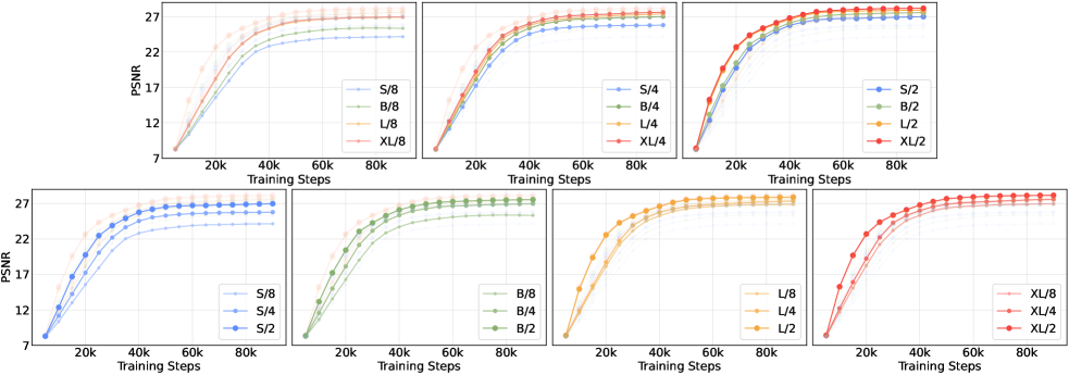
Figure 3: Scaling the ICDT model improves PSNR during the whole training process. We present PSNR over training steps for all 12 of our ICDT models. In the top row, we compare PSNR against model size while keeping patch size constant. In the bottom row, we compare PSNR against patch size while holding model size constant. Scaling the transformer backbone yields better generative models across all model sizes and patch sizes.

The results of Fig. 3 indicate that parameter counts is not the unique factor which determines the image enhancement quality of our models. As model size remains unchanged and patch size decreases, the overall amount of the transformer’s parameters is almost constant (slightly decreased actually), while only FLOPs increases. The results suggest that scaling model FLOPs is crucial to the performance of our models. To clarify this further, we plot the PSNR versus model FLOPs in Fig. 4. The results illustrate that different models have comparable performance in terms of PSNR if their total FLOPs are similar (e.g., ICDT-B/4 and ICDT-S/2). We observe a significant positive correlation between PSNR and model FLOPs, indicating that increased model computation is the key ingredient to improve the models’ performance. We observe the same trend in Fig. 1 of Supplementary Materials for other metrics such as SSIM.

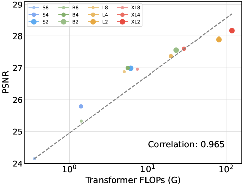
Figure 4: PSNR is strongly correlated with model FLOPs. We show PSNR of each ICDT model after 90K training iterations and each model’s FLOPs.

In Fig. 5, we plot PSNR against total training compute for all models, where training compute is approximately estimated as model FLOPs · batch size · training iterations · 3 (the factor of 3 approximates the backwards pass to be twice as compute-intensive as the forward pass). We find that models with small FLOPs (small model size or large patch size), despite being trained longer, eventually have inferior performance relative to models with large FLOPs trained for fewer iterations. For example, L/2 is outperformed by XL/2 after roughly 6.6 $\times$ 10⁸ GFLOPs. After sufficient training, computational intensive models behavior better even when controlling for total training FLOPs; that is to say, they are more compute-efficient.

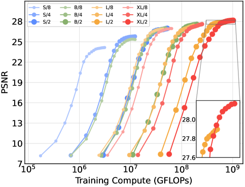
Figure 5: Larger ICDT models are more compute-efficient. We present PSNR against total training compute.

We illustrate the impact of scaling on sample quality in Fig. 6. At 90K training iterations, we sample an image from each of the 12 models using the same initial noise ${\bf{x}}_{T}$ and sampling noise. This visually demonstrates that increasing either model size or the number of tokens results in considerable improvements in visual quality.

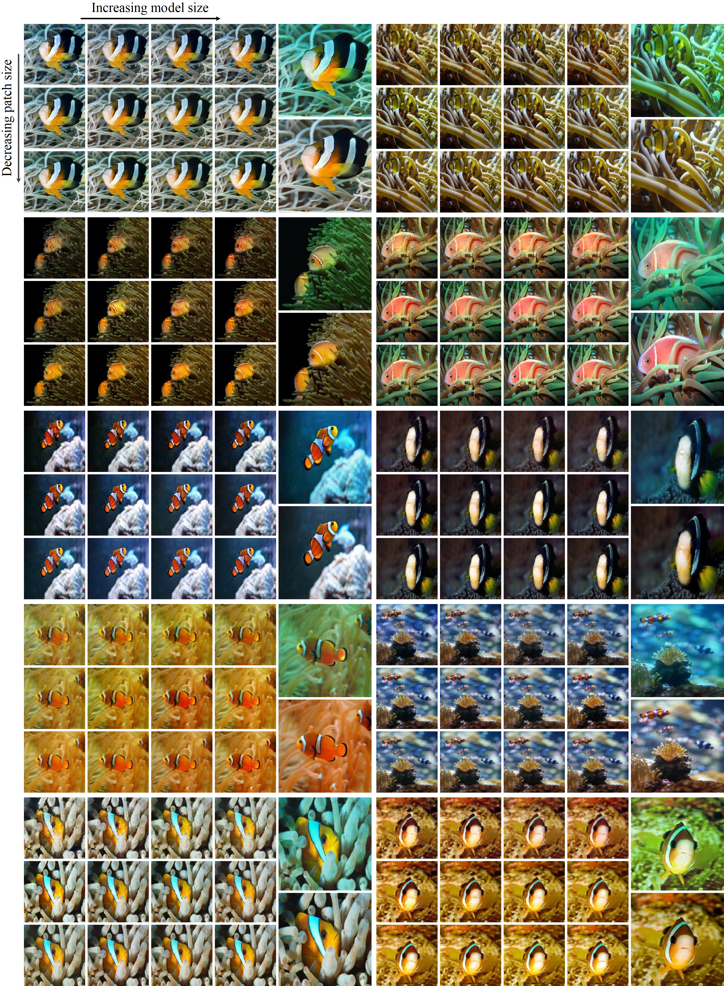
Figure 6: Increasing forward pass FLOPs of ICDT improves sample quality. Best viewed zoomed-in. Starting from the same input latent noise, we sample from all 12 of our ICDT models after 90K training iterations. The left 12 smaller images in a group (The 14 images containing the same content make up a group.) are the samples from each models, while the two enlarged images in the upper and lower right corners are the degraded image and the reference image, respectively. Increasing transformer depth/width or the number of input tokens, which equally increases the Gflops of models, achieves substantial improvements in visual quality.

V-B Comparison with Other UIE Methods

After analyzing the scalability, we compare the most computational intensive model, ICDT-XL/2, with SOTA UIE methods. These methods includes five CNN-based methods (Water-Net[12], UWCNN[13], Shallow-UWnet[14], UIECˆ2-Net[58], and RAUNE-Net[59]) as well as two GAN-based methods (FUnIEGAN[18] and MLFcGAN[19]).

We visualize several results in Fig. 7. In Fig. 7, the proposed ICDT effectively remits color casts and removes the haze on the underwater images, producing visually pleasing results. By contrast, the competing methods induce low brightness and contrast (e.g., UWCNN[13], UIECˆ2-Net[58], and FUnIEGAN[18]) or introduce blurring (e.g., UWCNN[13]), unexpected colors (e.g., MLFcGAN[19]), and artifacts (e.g., RAUNE-Net[59] and FUnIEGAN[18]).

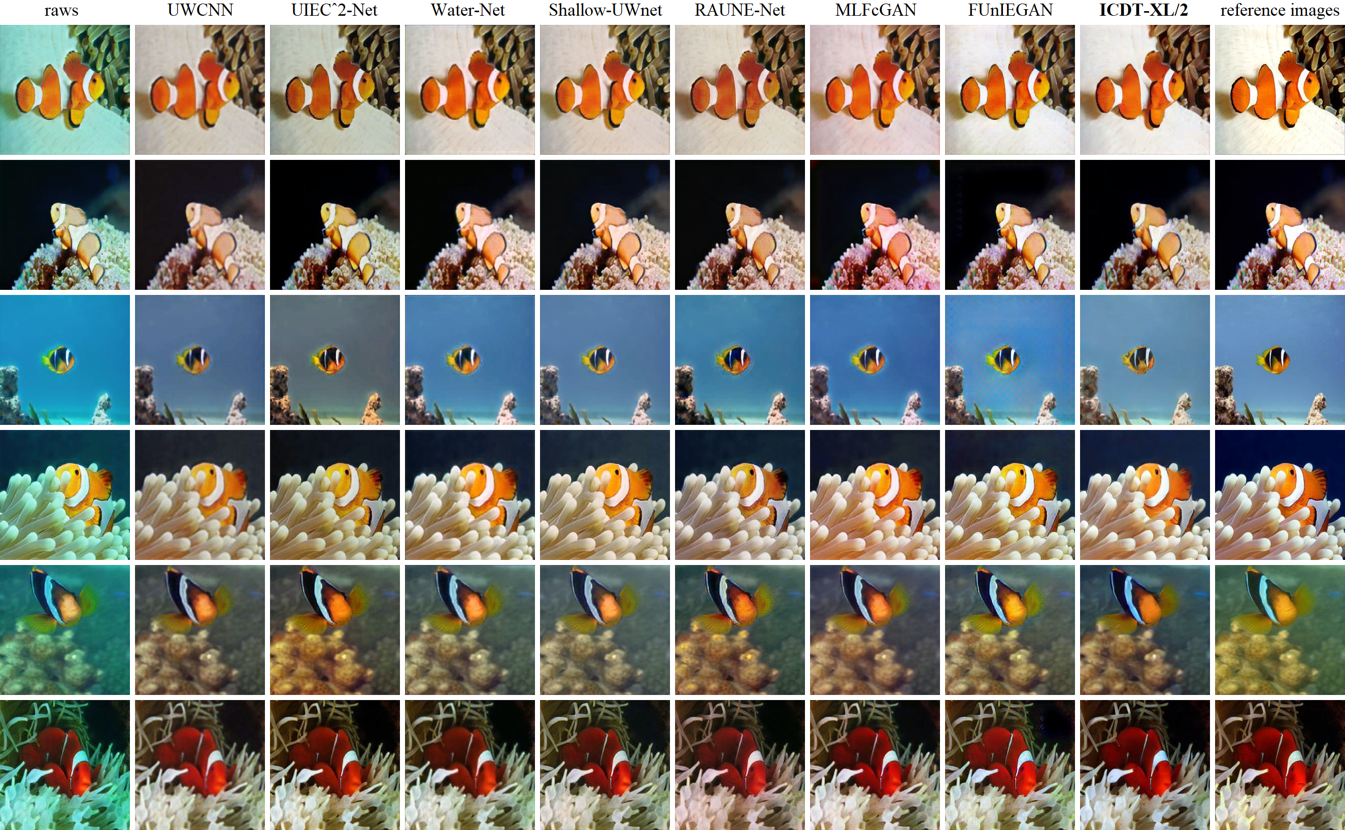
Figure 7: Qualitative comparisons of seven different UIE methods and our ICDT method. From left to right are raw images, the results of UWCNN[13], UIECˆ2-Net[58], Water-Net[12], Shallow-UWnet[14], RAUNE-Net[59], MLFcGAN[19], FUnIEGAN[18], the proposed ICDT-XL2, and reference images.

Table II reports the results of quantitative comparisons with SOTA UIE methods in terms of PSNR, SSIM, LPIPS, and UIQM. The full-reference image quality metrics PSNR, SSIM, and LPIPS are obtained through comparison between the result of each method and the corresponding reference image. DiT-XL/2 outperforms all competing methods, achieving the highest PSNR and SSIM as well as the lowest LPIPS. In addition, we observe that our DiT-XL/2 achieves the highest UIQM score of all prior UIE methods, indicating DiT-XL/2 also performs best in terms of non-reference image quality assessment.

TABLE II: Quantitative Comparisons with SOTA UIE Methods

Method	PSNR$\uparrow$	SSIM$\uparrow$	LPIPS$\downarrow$	UIQM$\uparrow$
UWCNN[13]	17.7347	0.7112	0.3911	2.6407
UIECˆ2-Net[58]	22.4930	0.8254	0.2932	2.7152
Water-Net[12]	25.4032	0.8355	0.2755	2.8481
Shallow-UWnet[14]	26.1325	0.8562	0.2359	2.8331
RAUNE-Net[59]	26.6946	0.8415	0.1990	2.8869
MLFcGAN[19]	21.6062	0.8246	0.3646	2.7195
FUnIEGAN[18]	24.1463	0.8233	0.1952	2.8239
ICDT-XL/2	28.1673	0.8744	0.1362	2.9234

Best and second best values are indicated with bold text and underlined

text respectively.

Qualitative and quantitative comparisons demonstrate the effectiveness of our ICDT method.

VI Conclusion

We introduce a novel ICDT model for UIE, which uses the degraded underwater image as the extra conditional input. ICDT employs a transformer backbone instead of the U-Net which is commonly used in DDPMs. As a result, ICDT inherits good scalability properties from the transformer model, enabling a trade-off between image enhancement quality and model complexity. Through comparisons against prior works, our largest ICDT model achieves SOTA image enhancement quality. Given the promising experimental results, we will continue to scale ICDTs to larger models and token counts in the future. Note that ICDT is a generic image-to-image generative model. With this understanding, this article can be regarded as taking UIE task as an example to interpret the working of ICDT. We leave it to future work to explore the application of ICDT in other image-to-image generation tasks.

References

- [1] W. Zhou, F. Zheng, G. Yin, Y. Pang, and J. Yi, “YOLOTrashCan: A deep learning marine debris detection network,” IEEE Trans. Instrum. Meas., vol. 72, pp. 1–12, Nov. 2023.
- [2] Q. Qi, Y. Zhang, F. Tian, Q. M. J. Wu, K. Li, X. Luan, D.Song, “Underwater image co-enhancement with correlation feature matching and joint learning,” IEEE Trans. Circuits Syst. Video Technol., vol. 32, no. 3, pp. 1133–1147, Mar. 2022.
- [3] S. Sun, H. Guo, G. Wan, C. Dong, C. Zheng, and Y. Wang, “High-precision underwater acoustic localization of the black box utilizing an autonomous underwater vehicle based on the improved artificial potential field,” IEEE Trans. Geosci. Remote Sens., vol. 61, pp. 1–10, Feb. 2023.
- [4] C. O. Ancuti, C. Ancuti, C. De Vleeschouwer, and P. Bekaert, “Color balance and fusion for underwater image enhancement,” IEEE Trans. Image Process., vol. 27, no. 1, pp. 379–393, Jan. 2018.
- [5] Z. Liang, X. Ding, Y. Wang, X. Yan, and X. Fu, “GUDCP: Generalization of underwater dark channel prior for underwater image restoration,” IEEE Trans. Circuits Syst. Video Technol., vol. 32, no. 7, pp. 4879–4884, Jul. 2022.
- [6] C.-Y. Li, J.-C. Guo, R.-M. Cong, Y.-W. Pang, and B. Wang, “Underwater image enhancement by dehazing with minimum information loss and histogram distribution prior,” IEEE Trans. Image Process., vol. 25, no. 12, pp. 5664–5677, Dec. 2016.
- [7] P. Drews, Jr. E. do Nascimento, F. Moraes, S. Botelho, and M. Campos, “Transmission estimation in underwater single images,” in Proc. IEEE Int. Conf. Comput. Vis. Workshops, 2013, pp. 825–830.
- [8] N. Wang, H. Zheng, and B. Zheng, “Underwater image restoration via maximum attenuation identification,” IEEE Access, vol. 5, pp. 18941–18952, Sep. 2017.
- [9] Y.-T. Peng, K. Cao, and P. C. Cosman, “Generalization of the dark channel prior for single image restoration,” IEEE Trans. Image Process., vol. 27, no. 6, pp. 2856–2868, Jun. 2018.
- [10] Z. Fu, W. Wang, Y. Huang, X. Ding, and K.-K. Ma, “Uncertainty inspired underwater image enhancement,” in Proc. 17th Eur. Conf. Comput. Vis., 2022, pp. 465–482.
- [11] X. Sun, L. Liu, Q. Li, J. Dong, E. Lima, and R. Yin, “Deep pixel-to-pixel network for underwater image enhancement and restoration,” IET Image Process., vol. 13, no. 3, pp. 469–474, 2019.
- [12] C. Li, C. Guo, W. Ren, R. Cong, J. Hou, S. Kwong, and D. Tao, ”An underwater image enhancement benchmark dataset and beyond,” IEEE Trans. Image Process., vol. 29, pp. 4376-4389, Feb. 2020.
- [13] C. Li, S. Anwar, and F. Porikli, “Underwater scene prior inspired deep underwater image and video enhancement,” Pattern Recognit., vol. 98, pp. 107038–107049, 2020.
- [14] A. Naik, A. Swarnakar, and K, Mittal, “Shallow-UWnet: Compressed model for underwater image enhancement,” in Proc. AAAI Conf. Artif. Intell., 2021, pp. 15853–15854.
- [15] C. Li, S. Anwar, J. Hou, R. Cong, C. Guo, and W. Ren, “Underwater image enhancement via medium transmission-guided multi-color space embedding,” IEEE Trans. Image Process., vol. 30, pp. 4985–5000, May 2021.
- [16] C. Fabbri, M. J. Islam, and J. Sattar, “Enhancing underwater imagery using generative adversarial networks,” in Proc. IEEE Int. Conf. Robot. Automat., 2018, pp. 7159–7165.
- [17] J. Li, K. A. Skinner, R. M. Eustice, and M. Johnson-Roberson, “WaterGAN: Unsupervised generative network to enable real-time color correction of monocular underwater images,” IEEE Robot. Autom. Lett., vol. 3, no. 1, pp. 387–394, Jan. 2018.
- [18] M. J. Islam, Y. Xia, and J. Sattar, “Fast underwater image enhancement for improved visual perception,” IEEE Robot. Automat. Lett., vol. 5, no. 2, pp. 3227–3234, Apr. 2020.
- [19] X. Liu, Z. Gao, and B. M. Chen, “MLFcGAN: Multilevel feature fusion-based conditional GAN for underwater image color correction,” IEEE Geosci. Remote Sens. Lett., vol. 17, no. 9, pp. 1488–1492, Sep. 2020.
- [20] G. Han, M. Wang, H. Zhu, and C. Lin, “UIEGAN: Adversarial learning-based photorealistic image enhancement for intelligent underwater environment perception,” IEEE Trans. Geosci. Remote Sens., vol. 61, pp. 1–14, May 2023.
- [21] R. Cong, W. Yang, W. Zhang, C. Li, C.-L. Guo, Q. Huang, and S. Kwong, “PUGAN: Physical model-guided underwater image enhancement using GAN with dual-discriminators,” IEEE Trans. Image Process., vol. 32, pp. 4472–4485, Jun. 2023.
- [22] H. Li, Y. Yang, M. Chang, H. Feng, Z. Xu, Q. Li, and Y. Chen, “Srdiff: Single image super-resolution with diffusion probabilistic models,” Neurocomputing, vol. 479, pp. 47–59, 2022.
- [23] C. Saharia, J. Ho, W. Chan, T. Salimans, D. J. Fleet, and M. Norouzi, “Image Super-Resolution via Iterative Refinement,” IEEE Trans. Pattern Anal. Mach. Intell., vol. 45, no. 4, pp. 4713–4726, Apr. 2023.
- [24] C. William, C. Huiwen, L. Chris, H. Jonathan, S. Tim, F. David, and N. Mohammad, “Palette: Image-to-image diffusion models,” in Proc. ACM SIGGRAPH Conf., 2022, pp. 1–10.
- [25] O. Ronneberger, P. Fischer, and T. Brox, “U-Net: Convolutional networks for biomedical image segmentation,” in Proc. Int. Conf. Med. Image Comput.-Assisted Intervention, 2015, pp. 234–241.
- [26] A. Dosovitskiy, L. Beyer, A. Kolesnikov, D. Weissenborn, X.-H. Zhai, T. Unterthiner, M. Dehghani, M. Minderer, G. Heigold, S. Gelly, J. Uszkoreit, and N. Houlsby, “An image is worth 16x16 words: Transformers for image recognition at scale,” in Proc. Int. Conf. Learn. Representations, 2021.
- [27] A. Nichol and P. Dhariwal, “Improved denoising diffusion probabilistic models,” in Proc. Int. Conf. Mach. Learn., 2021, pp. 8162–8171.
- [28] I. Goodfellow, J. Pouget-Abadie, M. Mirza, B. Xu, D. Warde-Farley, S. Ozair, A. Courville, and Y. Bengio, “Generative adversarial nets,” in Proc. Adv. Neural Inf. Process. Syst., 2014, pp. 2672–2680.
- [29] T. Karras, S. Laine, and T. Aila, “A style-based generator architecture for generative adversarial networks,” IEEE Trans. Pattern Anal. Mach. Intell., vol. 43, no. 12, pp. 4217–4228, Dec. 2021.
- [30] T. Karras, S. Laine, M. Aittala, J. Hellsten, J. Lehtinen, and T. Aila, “Analyzing and improving the image quality of StyleGAN,” in Proc. IEEE/CVF Conf. Comput. Vis. Pattern Recognit., 2020, pp. 8107–8116.
- [31] J. Ho, A. Jain, and P. Abbeel, “Denoising diffusion probabilistic models,” in Proc. Adv. Neural Inf. Process. Syst., 2020, pp. 6840–6851.
- [32] P. Dhariwal and A. Nichol, “Diffusion models beat GANs on image synthesis,” in Proc. Adv. Neural Inf. Process. Syst., 2021, pp. 8780–8794
- [33] A. Ramesh, P. Dhariwal, A. Nichol, C. Chu, and M. Chen, “Hierarchical text-conditional image generation with CLIP latents,” 2022, arXiv:2204.06125.
- [34] A. Nichol, P. Dhariwal, A. Ramesh, P. Shyam, P. Mishkin, B. McGrew, I. Sutskever, and M. Chen, “Glide: Towards photorealistic image generation and editing with text-guided diffusion models,” in Proc. Int. Conf. Mach. Learn., 2022, pp. 16784–16804.
- [35] R. Rombach, A. Blattmann, D. Lorenz, P. Esser, and B. Ommer, “High-resolution image synthesis with latent diffusion models,” in Proc. IEEE/CVF Conf. Comput. Vis. Pattern Recognit., 2022, pp. 10684–10695.
- [36] C. Saharia, W. Chan, S. Saxena, L. Li, J. Whang, E. Denton, S. Kamyar S. Ghasemipour, B. K. Ayan, S. S. Mahdavi, R. G. Lopes, T. Salimans, J. Ho, D. J Fleet, and M. Norouzi, “Photorealistic text-to-image diffusion models with deep language understanding,” in Proc. Adv. Neural Inf. Process. Syst., 2022, pp. 36479–36494.
- [37] J. Ho, C. Saharia, W. Chan, D. J. Fleet, M. Norouzi, and T. Salimans, “Cascaded diffusion models for high fidelity image generation,” J. Mach. Learn. Res., vol. 23, no. 47, pp. 1–33, Dec. 2022.
- [38] J. Song, C. Meng, and S. Ermon, “Denoising diffusion implicit models,” in Proc. Int. Conf. Learn. Representations, 2021.
- [39] T. Karras, M. Aittala, T. Aila, and S. Laine, “Elucidating the design space of diffusion-based generative models,” in Proc. Adv. Neural Inf. Process. Syst., 2022, pp. 26565–26577.
- [40] M. Mardani, J. Song, J. Kautz, and A. Vahdat, “A variational perspective on solving inverse problems with diffusion models,” 2023, arXiv:2305.04391.
- [41] O. Özdenizci and R. Legenstein, “Restoring vision in adverse weather conditions with patch-based denoising diffusion models,” IEEE Trans. Pattern Anal. Mach. Intell., vol. 45, no. 8, pp. 10346–10357, Aug. 2023.
- [42] B. Kawar, M. Elad, S. Ermon, and J. Song, “Denoising diffusion restoration models,” in Proc. Adv. Neural Inf. Process. Syst., 2022, pp. 23593–23606.
- [43] S. Lu, F. Guan, H. Zhang, and H. Lai, “Underwater image enhancement method based on denoising diffusion probabilistic model,” J. Vis. Commun. Image Representation, vol. 96, 2023.
- [44] S. Lu, F. Guan, H. Zhang, and H. Lai, “Speed-Up DDPM for real-time underwater image enhancement,” IEEE Trans. Circuits Syst. Video Technol., to be published, doi: 10.1109/TCSVT.2023.3314767.
- [45] A. Jabri, D. Fleet, and T. Chen, “Scalable adaptive computation for iterative generation,” 2022, arXiv:2212.11972.
- [46] D. P. Kingma and M. Welling, “Auto-encoding variational bayes,” 2013, arXiv:1312.6114.
- [47] W. Peebles and S. Xie, “Scalable diffusion models with transformers,” in Proc. IEEE/CVF Int. Conf. Comput. Vis., 2023, pp. 4195–4205.
- [48] X. Zhai, A. Kolesnikov, N. Houlsby, and L. Beyer, “Scaling vision transformers,” in Proc. IEEE/CVF Conf. Comput. Vis. Pattern Recognit., 2022, pp. 12104–12113.
- [49] D. Kingma and J. Ba, “Adam: A method for stochastic optimization,” in Proc. Int. Conf. Learn. Representations, 2015.
- [50] I. Loshchilov and F. Hutter, “Decoupled weight decay regularization,” 2017, arXiv:1711.05101.
- [51] A. Steiner, A. Kolesnikov, X. Zhai, R. Wightman, J. Uszkoreit, and L. Beyer, “How to train your ViT? data, augmentation, and regularization in vision transformers,” Trans. Mach. Learn. Res., 2022.
- [52] T. Xiao, P. Dollar, M. Singh, E. Mintun, T. Darrell, and R. Girshick, “Early convolutions help transformers see better,” in Proc. Adv. Neural Inf. Process. Syst., 2021, pp. 30392–30400.
- [53] Y. Song and S. Ermon, “Improved techniques for training score-based generative models,” in Proc. Adv. Neural Inf. Process. Syst., 2020, pp. 12438-12448.
- [54] Q. Huynh-Thu and M. Ghanbari, “Scope of validity of PSNR in image/video quality assessment,” Electron. Lett., vol. 44, no. 13, pp. 800–801, Jun. 2008.
- [55] Z. Wang, A. C. Bovik, H. R. Sheikh, and E. P. Simoncelli, “Image quality assessment: From error visibility to structural similarity,” IEEE Trans. Image Process., vol. 13, no. 4, pp. 600–612, Apr. 2004.
- [56] R. Zhang, P. Isola, A. A. Efros, E. Shechtman, and O. Wang, “The unreasonable effectiveness of deep features as a perceptual metric,” in Proc. IEEE/CVF Conf. Comput. Vis. Pattern Recognit., 2018, pp. 586–595.
- [57] K. Panetta, C. Gao, and S. Agaian, “Human-visual-system-inspired underwater image quality measures,” IEEE J. Ocean. Eng., vol. 41, no. 3, pp. 541–551, Jul. 2015.
- [58] Y. Wang, J. Guo, H. Gao, and H. Yue, “UIECˆ2-Net: CNN-based underwater image enhancement using two color space,” Signal Processing: Image Commun., vol. 96, 2021, Art. no. 116250.
- [59] W. Peng, C. Zhou, R. Hu, J. Cao, and Y. Liu, “RAUNE-Net: A residual and attention-driven underwater image enhancement method,” 2023, arXiv:2311.00246.