Learning Motion Blur Robust Vision Transformers with Dynamic Early Exit for Real-Time UAV Tracking

Abstract

Recently, the surge in the adoption of single-stream architectures utilizing pre-trained ViT backbones represents a promising advancement in the field of generic visual tracking. By integrating feature extraction and fusion into a cohesive framework, these architectures offer improved performance, efficiency, and robustness. However, there has been limited exploration into optimizing these frameworks for UAV tracking. In this paper, we boost the efficiency of this framework by tailoring it into an adaptive computation framework that dynamically exits Transformer blocks for real-time UAV tracking. The motivation behind this is that tracking tasks with fewer challenges can be adequately addressed using low-level feature representations. Simpler tasks can often be handled with less demanding, lower-level features. This approach allows the model use computational resources more efficiently by focusing on complex tasks and conserving resources for easier ones. Another significant enhancement introduced in this paper is the improved effectiveness of ViTs in handling motion blur, a common issue in UAV tracking caused by the fast movements of either the UAV, the tracked objects, or both. This is achieved by acquiring motion blur robust representations through enforcing invariance in the feature representation of the target with respect to simulated motion blur. The proposed approach is dubbed BDTrack. Extensive experiments conducted on five tracking benchmarks validate the effectiveness and versatility of our approach, establishing it as a cutting-edge solution in real-time UAV tracking. Code is released at: https://github.com/wuyou3474/BDTrack.

I Introduction

Unmanned Aerial Vehicle (UAV) tracking involves the process of determining and predicting the location and size of a specific object in successive aerial images. This capability has become increasingly essential in a variety of fields, such as public safety, disaster management, environmental monitoring, industrial inspections, and agriculture, due to its wide-ranging applications and benefits [1, 49, 18, 4, 12, 2]. Despite its benefits, UAV tracking faces significant challenges, including extreme viewing angles that require robust algorithms to handle diverse perspectives, severe motion blur from rapid UAV movement that complicates the tracking process, and significant occlusions where objects are obscured by other elements. Additionally, UAVs have limited computational resources and battery life, necessitating highly efficient tracking algorithms to ensure sustained and accurate operation during missions [5, 6]. Therefore, a practical tracker must ensure accurate tracking while addressing the computational and power constraints of the UAVs. Although discriminative correlation filters (DCF)-based trackers are widely used in UAV tracking for their efficiency [7, 9, 11, 3], their tracking precision often lags behind that of deep learning (DL)-based methods [49, 5, 4, 12]. A recent trend in the generic tracking community sees a growing preference for single-stream architectures, seamlessly integrating feature extraction and correlation using pre-trained Vision Transformer (ViT) backbone networks [13, 14, 17, 8], showcasing notable success. In line with this trend, Aba-ViTrack [18] presents an efficient DL-based tracker that utilizes this framework. It includes an adaptive and background-aware token computation method to reduce inference time, demonstrating impressive precision and speed, making it a state-of-the-art (SOTA) tracker for real-time UAV tracking. However, the varying token number of this method entails unstructured access operations, resulting in a notable time costs. In our research, we employ the same single-stream architecture, but our focus is on enhancing the efficiency of ViTs through more structured methods: the early exiting strategy.

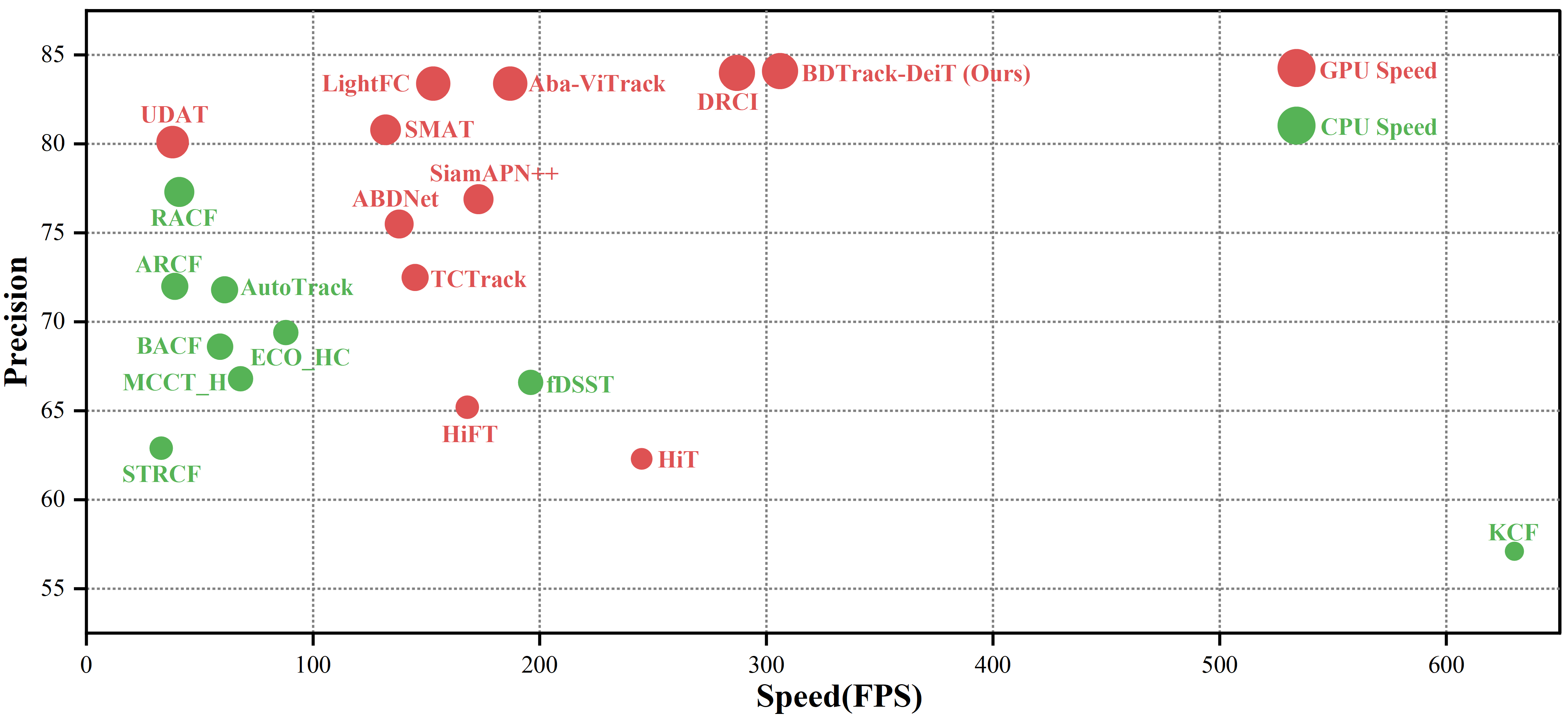
Figure 1: Compared with state-of-the-art UAV tracking algorithms on UAVDT. Our BDTrack-DeiT sets a new record with 0.841 precision and still runs efficiently at around 305 FPS.

Early exiting is a technique designed to expedite the processing of input data by allowing a model to terminate its forward pass prematurely based on certain criteria, reducing computational costs without compromising much predictive accuracy, especially if the behavior or characteristics of the task vary based on the specific examples or instances involved. This approach has gained traction in various domains, especially in real-time applications and resource-constrained environments, and a number of studies have explored its implications [19, 20, 21, 40, 22]. Research in this area explores various strategies, including adaptive methods that dynamically assess model confidence [19, 22], distillation [23], architecture design [24, 21], and training scheme [20, 40]. This approach has been applied across various deep learning architectures, including convolutional neural networks (CNNs) [19, 23], recurrent neural networks (RNNs) [24], and Transformer-based models [21, 22]. While it has found success in applications ranging from natural language processing [24, 40] to many vision tasks (e.g., image classification [22], video recognition [25], and image captioning [26]) and vision language learning [27], its potential for enhancing efficiency in UAV tracking has not been explored to the best of our knowledge. In this work, we introduce a Dynamic Early Exit Module (DEEM) to streamline the architecture of ViTs and enhance the efficiency of the inference process for real-time UAV tracking. Given that the tracking challenge for a specific target is context-dependent, the adaptive neglect of high-level ViT blocks can significantly reduce unnecessary high-level semantic features without significantly affecting the performance of the tracker.

In addition, this research also aims to enhance the performance of UAV trackers by mitigating the adverse effects of motion blur, which is a prevalent challenge in UAV tracking as rapid and unpredictable movements of UAVs are common due to factors such as wind, changes in altitude, sudden maneuvers, or the need to track fast-moving targets [11, 6, 28]. Although numerous methods aiming to address motion blur in visual tracking have been proposed [29, 30, 31, 32, 33], their broad applicability is impeded by significant drawbacks. Their intricate designs, complex architectures [34, 33], or training procedures [31, 33], present implementation challenges and requires substantial computational resources. Moreover, many of them neglect efficiency considerations [29, 30, 32], rendering them less suitable for resource-constrained scenarios such as real-time UAV tracking. Simplifying the design and ensuring efficiency are pivotal for increasing the adoption and effectiveness of methods designed to tackle motion blur in UAV tracking, especially for real-time needs. In this work, we propose to learn motion blur robust feature representations with ViTs by minimizing the mean square error (MSE) between the feature representation of the original template and its blurred version subject to motion blur. Our approach distinguishes itself through its simplicity, avoiding the inclusion of extra architectural complexities. Instead, it introduces a straightforward yet effective enhancement by incorporating only an additional loss. This enhancement can be seamlessly integrated into other tracking methods to bolster robustness against motion blur, which imposes no extra computational burden during the inference phase, making it particularly well-suited for real-time UAV tracking scenarios where efficiency is crucial. It is worth noting that the targets subjecting to motion blur is simulated considering that this manner can be conducted on-demand and provides a cost-effective and scalable solution, among other advantages [35]. The proposed framework is called BDTrack. Validation using real-world data demonstrates that our method significantly enhances the robustness against motion blur of baseline methods. Remarkably, our BDTrack-DeiT outperforms the SOTA tracker ABDNet [33], which was proposed to address motion blur, by 5.5% in precision on the motion blur subset of the UAVDT dataset with more than 2 times faster GPU speed (See Fig. 4 and Table I). Extensive experiments on five benchmarks show that our method achieves SOTA performance. As shown in Fig. 1, our method sets a new record with a precision of 0.841 and runs efficiently at around 305 frames per second (FPS) on the UAVDT. The following is a summary of our contributions:

• We introduce a novel module that adaptively streamlines the architecture of Vision Transformers (ViTs) by dynamically exiting Transformer blocks. Our method is straightforward and can significantly enhance the efficiency of baseline ViT-based UAV tracking methods with minimal impact on their tracking performance.

• We make the first attempt to learn motion blur robust ViTs by enforcing invariance in the feature representation of the target against simulated motion blur using simply a mean square error (MSE) loss. Our approach incurs no additional computational burden during the inference, making it well-suited for real-time UAV tracking.

• We present BDTrack, an efficient tracker seamlessly integrating these components, which is readily integrable into similar ViT-based trackers. BDTrack is able to maintain high tracking speeds while delivering exceptional performance. Extensive experiments on five benchmarks confirm its state-of-the-art performance.

The remainder of this paper is structured as follows: Section II provides an overview of previous research related to this study. In Section III, we describe the methodology of the proposed technique in detail. Section IV outlines the experiments conducted and discusses their results. Finally, Section V presents the conclusions and insights drawn from the paper.

II Related Work

II-A Motion Blur Aware Trackers

Motion blur presents a significant challenge in visual tracking, and various approaches have been proposed to address this issue and enhance the robustness of tracking algorithms [10, 30, 31, 32, 33], including employing specialized architectures or mechanisms to handle motion blur, learning motion blur robust representations, and combining motion deblurring techniques. For example, Ding et al. [10] introduce a method to enhance the robustness of the appearance model against severe blur by incorporating various blur kernels during the training process. Guo et al. [32] propose a novel Generative Adversarial Network (GAN)-based scheme aimed at enhancing tracker robustness to motion blurs. To address the challenges posed by motion blur in UAV tracking, Zuo et al. [33] introduced the Tracking-Oriented Adversarial Blur-Deblur Network (ABDNet) very recently, which includes a novel deblurring component to restore the visual appearance of blurred targets and an innovative blur generator that creates realistic blurry images for adversarial training. While existing methods have shown success in addressing motion blur in visual tracking, their implementation is complex and the efficiency of the algorithms is not a primary consideration. This complexity and inefficiency make these methods unsuitable for real-time UAV tracking scenarios, where computational resources and time are limited. In this study, we introduce motion blur robust ViTs for UAV tracking by learning motion blur invariant feature representations in a simpler and more efficient manner. Our approach is designed to incur no additional computational burden during the inference phase, making it exceptionally well-suited for real-time UAV tracking scenarios where efficiency is paramount. Furthermore, our method can be easily adapted to other ViT-based tracking methods, enhancing their performance in the presence of motion blur without compromising speed or computational efficiency.

II-B Efficient Vision Transformers

Efforts to enhance the efficiency of ViTs have garnered significant attention in recent years, driven by the need to reconcile their powerful representation capabilities with computational efficiency. One avenue of exploration involves the design of lightweight ViT architectures, employing techniques such as low-rank methods, model compression, and hybrid designs [16, 36, 37]. However, Low-rank and quantization-based ViTs often trade substantial accuracy for efficiency gains. Pruning-based ViTs typically require intricate decisions on pruning ratios and involve a time-consuming fine-tuning process. Hybrid ViTs featuring CNN-based stems impose limitations on input size flexibility, preventing the simultaneous input of images with varying dimensions [18].

With the increased popularity, efficient ViTs based on conditional computation have very recently explored adaptive inference for model acceleration, which dynamically adjust the computational load based on input complexity, enabling ViTs to allocate resources judiciously during inference. For instance, DynamicViT [38] introduces extra control gates to pause specific tokens using the Gumbel-softmax trick. A-ViT [39] adopts an Adaptive Computation Time (ACT)-like approach to eliminate the need for extra halting sub-networks, resulting in simultaneous improvements in efficiency, accuracy, and token importance allocation. A-ViT was also exploited in Aba-ViTrack [18] to built efficient trackers for real-time UAV tracking. However, its variable number of tokens incurs considerable time cost due to additional unstructured assess operations. More structured methods can resort to early exiting that leverage dynamic early exiting strategies to improve inference efficiency of Transformer models, as demonstrated in [40, 26, 27, 22]. Nevertheless, these studies primarily focus on large-scale models and incorporate inefficient architectures or training methods for making early exiting decisions. These criteria for early exiting are challenging to adapt effectively to lightweight models. For example, the early exiting strategy proposed for vision language models in [27] relies on layer-wise Cosine similarities. While Cosine similarities have proven effective for large-scale models characterized by high-level and high-dimensional feature representations, their performance may be suboptimal in lightweight models where non-linearities and complex dependencies are challenging to linearize or trivialize [41, 42]. The dynamic early exiting method proposed for accelerating ViTs in [22] involves training delicate Local Perception and Global Aggregation Heads separately with distinct supervisions. However, this intricate training setup introduces significant inefficiencies into the training process. In this work, we explore a more structured and efficient approach to dynamically early exit ViT blocks by incorporating a dynamic early exit module. Our method aims to simplify the training process, improve inference efficiency, and maintain adaptability across different ViT-based models.

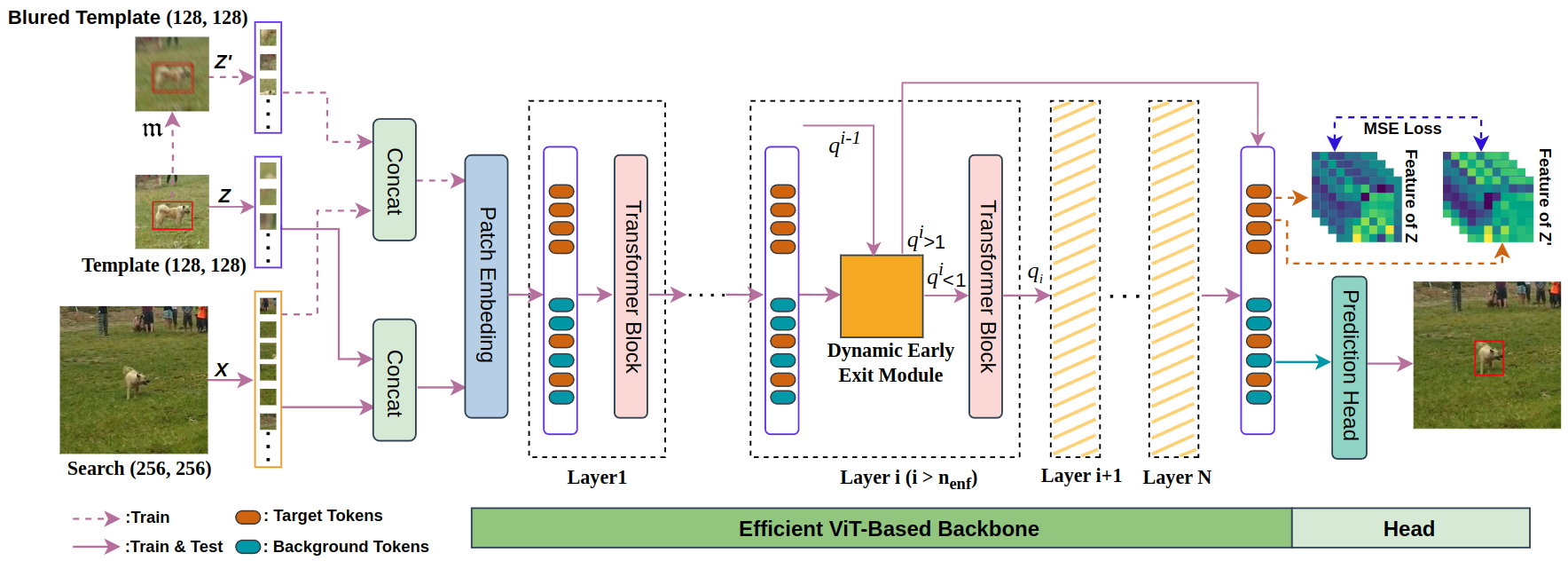
Figure 2: Overview of our BDTrack. It comprises of a single-stream backbone and a prediction head. Simulated blurred templates and Dynamic Early Exit Modules (see Fig. 3) are employed to learn motion blur robust representations and to boost efficiency, respectively.

III Method

In this section, we first briefly overview our tracking framework, BDTrack, as illustrated in Fig. 2. Then, we introduce the proposed method for learning motion blur robust ViTs (MBRV) and the dynamic early exit module (DEEM). Finally, we detail the prediction head and training objective.

III-A Overview

Our BDTrack is a tracking framework that employs a single-stream approach, taking the target template and the search image as inputs. This framework consists of an adaptive ViT-based backbone and a prediction head. The features extracted from the backbone are subsequently forwarded to the prediction head to achieve tracking predictions. To enhance the robustness of ViTs against motion blur, we minimize the Mean Squared Error (MSE) between the feature representations of the target template and its blurred counterpart. The blurred version of the template is generated using the linear motion blur method, as referenced in [35]. This approach aims to ensure that the ViTs can maintain consistent performance even when the input images are affected by motion blur, a common issue in UAV tracking. Additionally, to further enhance the efficiency of ViTs, we introduce a dynamic early exit module (DEEM) for each ViT block (layer), excluding the initial $n_{enf}$ blocks. This module is trained to dynamically predicts the exiting score $\mathfrak{e}^{l}$ at the $l$-th layer. The forward pass of the ViT exists at layer $l$ when the cumulative exiting score exceeds a certain threshold. This mechanism allows the model to allocate computational resources more efficiently, exiting early for simpler tasks and reserving full processing power for more complex ones. The details of the two components will be elaborated in the subsequent subsections.

III-B Learning Motion Blur Robust ViTs (MBRV)

A motion blur robust ViT (MBRV) serves as a pivotal component in our pursuit of a compact and efficient end-to-end tracker specifically designed for real-time UAV tracking. In the context of UAV tracking, where rapid and accurate object localization is paramount, the presence of motion blur in captured images poses a significant challenge. Motion blur can distort object features, leading to inaccuracies in tracking algorithms and potentially compromising the effectiveness of the entire tracking system. The inclusion of MBRV addresses these challenges by ensuring that the ViT-based backbone of our tracking system remains effective even in the presence of motion blur. By minimizing the Mean Squared Error (MSE) between the feature representations of the target template and its blurred counterpart, MBRV enhances the robustness of the tracker. Furthermore, the compact and efficient nature of MBRV aligns with our goal of developing a tracker optimized for real-time UAV tracking.

During the training phase, the MBRV receives three inputs: a target template $Z$, a blurred target template $Z^{\prime}$= $\mathfrak{m}(Z)$, and a search image $X$, where $\mathfrak{m}(Z)$ represents applying simulated motion blur to the template image $Z$ using the linear motion blur method implemented in [43]. The input images are first segmented and then flattened into sequences of patches. Subsequently, the sequences corresponding to $Z$ and $X$ are concatenated into an ordered sequence denoted by $[Z,X]$. The same procedure is applied to the sequences corresponding to $Z^{\prime}$ and $X$, leading to $[Z^{\prime},X]$. In the forward pass, $[Z,X]$ is tokenized by a trainable linear projection layer $\mathfrak{E}$ called patch embedding, which generates $\mathcal{K}$ tokens as follows:

$$\textbf{t}_{1:\mathcal{K}}^{0}=\mathfrak{E}([Z,X])\in\mathbb{R}^{\mathcal{K}\times d},$$ (1)

where the embedding dimension of each token is denoted by $d$, and the token sequences $t^{0}_{1:\mathcal{K}z}$ and $t^{0}_{\mathcal{K}_{z}+1:\mathcal{K}}$ ($1<\mathcal{K}_{z}<\mathcal{K}_{x}<\mathcal{K}$) correspond to the template and search image, respectively, where $\mathcal{K}=\mathcal{K}_{z}+\mathcal{K}_{x}$. The $\mathcal{K}$ tokens $\textbf{t}_{1:\mathcal{K}}^{0}$ are then input into the Transformer blocks to obtain their final feature representations. Let $\mathfrak{F}^{l}$ represent the Transformer block at layer $l$, transforming all tokens from layer $(l-1)$ as $\textbf{t}_{1:\mathcal{K}}^{l}=\mathfrak{F}^{l}(\textbf{t}_{1:\mathcal{K}}^{l-1})$. The overall MBRV of $L$ ViT blocks in total, denoted by $\mathfrak{B}$, can be expressed as:

$$\textbf{t}_{1:\mathcal{K}}^{L}(Z,X)=\mathfrak{B}(Z,X)=\mathfrak{F}^{L}\circ\mathfrak{F}^{L-1}\circ...\circ\mathfrak{F}^{1}\circ\mathfrak{E}([Z,X]),$$ (2)

where $\circ$ denotes the composition operation. Similarly, we can derive the feature representation of $[Z^{\prime},X]$. As $[Z,X]$ and $[Z^{\prime},X]$ are ordered sequences of tokens, the feature representation of $Z$ and $Z^{\prime}$ can be retrieved by tracking their token indices in the respective ordered sequences, specifically denoted as $\textbf{t}_{1:\mathcal{K}z}^{L}(Z,X)$ and $\textbf{t}_{1:\mathcal{K}_{z}}^{L}(Z^{\prime},X)$, respectively. The core idea behind MBRV is to minimize the mean square error between the feature representation of $Z$ and that of $Z^{\prime}$. This is achieved by minimizing the following MSE loss:

$$\mathcal{L}_{br}=||\textbf{t}_{1:\mathcal{K}_{z}}^{L}(Z,X)-\textbf{t}_{1:\mathcal{K}_{z}}^{L}(Z^{\prime},X)||^{2}.$$ (3)

During the inference phase, only the sequence $[Z,X]$ is input to the MBRV, there is no need for simulating motion blur. Consequently, our method does not introduce any additional computational cost in the inference phase. Notably, our method is agnostic to the specific ViTs employed, allowing seamless integration with any ViTs within our framework.

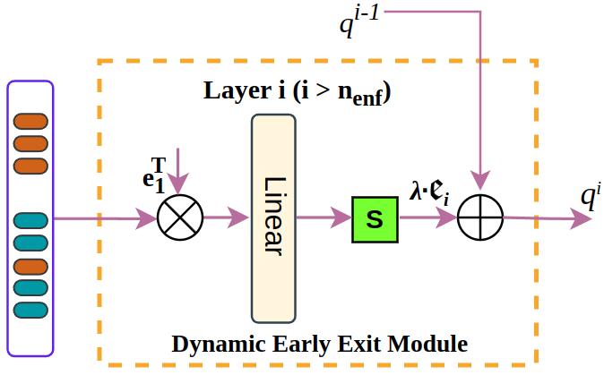
Figure 3: The detailed structure of the Dynamic Early Exit Module.

III-C Dynamic Early Exit Module (DEEM)

The primary goal of the DEEM is to allocate computational resources in a dynamic manner based on the complexity of each VIT block’s input, aiming to enhance inference efficiency while preserving performance. The DEEM operates by dynamically assessing the complexity of the input at each ViT block and making decisions regarding whether to continue processing or to exit early. This decision-making process is based on predefined criteria, specifically the cumulative exiting score exceeding a certain threshold. By exiting early for simpler inputs and reserving computational resources for more complex ones, the module optimizes the overall efficiency of the tracking system. While the primary objective of the DEEM is to improve inference efficiency, it does so without sacrificing tracking performance. The module is designed to ensure that early exits occur only when appropriate, thereby maintaining the accuracy and reliability of the tracking predictions. This balance between efficiency and performance is essential in real-time UAV tracking systems.

The DEEM is accomplished by employing a linear layer in conjunction with a non-linear activation function, with a slice of all tokens representing both the target template and the search image as its input, as illustrated in Fig. 3. Its output represents the exiting score at the corresponding ViT block (layer). Specifically, take the $i$-th ($i>n_{enf}$) layer for example, the slice of all tokens ouput by the $(i-1)$-th ViT block is denoted by $\textbf{e}_{1}^{\textup{T}}\textbf{t}_{1:\mathcal{K}}^{i-1}(Z,X):=\textbf{b}^{i-1}\in\mathbb{R}^{\mathcal{K}}$, where $\textbf{e}_{1}^{\textup{T}}=[1,0,...,0]\in\mathbb{R}^{\mathcal{K}}$ is a standard unit vector in $\mathbb{R}^{\mathcal{K}}$, the linear layer is denoted by $\mathfrak{l}^{i}$, where $d$ is the token dimension. Formally the DEEM at layer $i$ is defined by $\mathfrak{e}^{i}=\mathfrak{s}(\mathfrak{l}^{i}(\textbf{b}^{i-1}))$, where $\mathfrak{e}^{i}\in[0,1]$ represents the exiting score of the $i$-th Transformer block, $\mathfrak{s}(x)=1/(1+e^{-x})$ denotes the sigmoid function. The forward pass exits if the cumulative exiting score $q^{i}=\sum_{k=n_{enf}+1}^{i}\lambda\mathfrak{e}^{k}$ exceeds $1-\epsilon$, i.e., $q^{i}\geqslant 1-\epsilon$, where $\epsilon$ is a small positive constant that allows exiting after examing one DEEM module. Note that, if $n_{enf}=0$, theoretically all $L$ blocks could be skipped simultaneously, resulting in no correlation computation between the template and search image. To prevent such an undesirable case, the first $n_{enf}>0$ layers are enforced without examination. This strategy is implemented to reduce computational burdens because these low-level blocks are expected in most cases, as low-level features provide foundational information upon which more complex features and representations can be built. Another extreme case is that, for any input, early exit never happens as by which the model is easier to reduce the training losses with more ViT blocks. To address this, we introduce a block sparsity loss, denoted as $\mathcal{L}_{spar}$, which penalizes smaller average exiting scores over all examined layers. This encourages, on average, an earlier exit during the forward pass to enhance efficiency. Let $L_{e}$ be the maximum layer of examined ViT blocks, it follows that

$$L_{e}=\underset{n_{enf}<n\leqslant L}{\textup{argmin}}\left\{\sum_{l=n_{enf}+1}^{n}\mathfrak{e}^{l}\geqslant 1-\varepsilon\right\}.$$ (4)

The block sparsity loss is formally defined as follows:

$$\begin{split}\mathcal{L}_{spar}=||\frac{1}{L_{e}-n_{enf}}\sum^{L_{e}}_{l=n_{enf}+1}\mathfrak{e}^{l}-\tau||^{2},\end{split}$$ (5)

where $\tau$ is a constant used along with $\lambda$ to control the block sparsity. We call $\tau$ the block sparsity constant. Given $\lambda$, generally the larger $\tau$ is, the more sparse the model will be.

III-D Prediction Head and Training Objective

Following [13], we utilize a fully convolutional network-based prediction head $\mathcal{C}$, consisting of multiple Conv-BN-ReLU layers. The output tokens $t^{L_{e}}_{\mathcal{K}_{z}+1:\mathcal{K}}$ associated with the search image are first reinterpreted into a 2D spatial feature map, which is then input to the prediction head. The head generates three outputs: a target classification score $\mathbf{p}\in[0,1]^{H_{x}/P\times W_{x}/P}$, a local offset $\mathbf{o}\in[0,1]^{2\times H_{x}/P\times W_{x}/P}$, and a normalized bounding box size $\mathbf{s}\in[0,1]^{2\times H_{x}/P\times W_{x}/P}$. The highest classification score is used to estimate the coarse target position, i.e., $(x_{c},y_{c})=\textup{argmax}_{(x,y)}\mathbf{p}(x,y)$, based on which the final target bounding box is determined by

$$\{(x_{t},y_{t});(w,h)\}=\{(x_{c},y_{c})+\mathbf{o}(x_{c},y_{c});\mathbf{s}(x_{c},y_{c})\}.$$ (6)

For the tracking task, we employ the weighted focal loss [59] for classification and a combination of $L_{1}$ loss and GIoU loss [60] for bounding box regression. The overall loss function is formulated as:

$$\mathcal{L}_{overall}=\mathcal{L}_{cls}+\eta_{iou}\mathcal{L}_{iou}+\eta_{L_{1}}\mathcal{L}_{L1}+\rho\mathcal{L}_{br}+\gamma\mathcal{L}_{spar}$$ (7)

where the constants $\eta_{iou}=2$ and $\eta_{L_{1}}=5$ are the same as in [13], $\rho$ and $\gamma$ are set to $10^{-4}$ and $10^{3}$ respectively. Our framework is trained end-to-end with the overall loss $\mathcal{L}_{overall}$ after the pretrained weights of the ViT for image classification is loaded.

TABLE I: Comparison of precision (Prec.), success rate (Succ.), and speed (FPS) between BDTrack and lightweight trackers on five UAV tracking benchmarks, namely DTB70, UAVDT, VisDrone2018, UAV123, and UAV123@10fps. Red, blue and green indicate the first, second and third place. It is worth noting that the percent symbol (%) has been omitted for Prec. and Succ. values.

			DTB70		UAVDT		VisDrone		UAV123		UAV123@10fps		Avg.		Avg.FPS
Method		Source	Prec.	Succ.	Prec.	Succ.	Prec.	Succ.	Prec.	Succ.	Prec.	Succ.	Prec.	Succ.	GPU	CPU
	KCF[7]	TPAMI 15	46.8	28.0	57.1	29.0	68.5	41.3	52.3	33.1	40.6	26.5	53.1	31.6	-	622.5
	BACF[44]	ICCV 17	58.1	39.8	68.6	43.2	77.4	56.7	66.0	45.9	57.2	41.3	65.5	45.4	-	54.2
	fDSST[45]	TPAMI 17	53.4	35.7	66.6	38.3	69.8	51.0	58.3	40.5	51.6	37.9	60.0	40.7	-	193.4
	ECO_HC[46]	CVPR 17	63.5	44.8	69.4	41.6	80.8	58.1	71.0	49.6	64.0	46.8	69.7	48.2	-	83.5
	MCCT_H[47]	CVPR 18	60.4	40.5	66.8	40.2	80.3	56.7	65.9	45.7	59.6	43.4	66.6	45.3	-	63.4
	STRCF[48]	CVPR 18	64.9	43.7	62.9	41.1	77.8	56.7	68.1	48.1	62.7	45.7	67.3	47.1	-	28.4
	ARCF[9]	ICCV 19	69.4	47.2	72.0	45.8	79.7	58.4	67.1	46.8	66.6	47.3	71.0	49.1	-	34.2
	AutoTrack[11]	CVPR 20	71.6	47.8	71.8	45.0	78.8	57.3	68.9	47.2	67.1	47.7	71.6	49.0	-	57.8
DCF-based	RACF[6]	PR 22	72.6	50.5	77.3	49.4	83.4	60.0	70.2	47.7	69.4	48.6	74.6	51.2	-	35.6
	HiFT[1]	ICCV 21	80.2	59.4	65.2	47.5	71.9	52.6	78.7	59.0	74.9	57.0	74.2	55.1	160.3	-
	SiamAPN++[49]	IROS 21	78.9	59.4	76.9	55.6	73.5	53.2	76.8	58.2	76.4	58.1	76.5	56.9	167.5	-
	LightTrack[50]	CVPR 21	76.4	59.1	80.4	61.2	74.8	56.8	78.3	62.7	75.1	59.9	77.0	59.9	121.4	-
	HCAT[58]	ECCV 22	83.5	63.7	74.2	54.3	75.4	57.7	83.0	67.8	81.9	64.4	79.6	61.6	144.4	-
	TCTrack[5]	CVPR 22	81.2	62.2	72.5	53.0	79.9	59.4	80.0	60.5	78.0	59.9	78.3	59.0	139.6	-
	UDAT[55]	CVPR 22	80.6	61.8	80.1	59.2	81.6	61.9	76.1	59.0	77.8	58.5	79.2	60.1	33.7	-
	SGDViT[56]	ICRA 23	78.5	60.4	65.7	48.0	72.1	52.1	75.4	57.5	86.3	66.1	75.6	56.8	110.5	-
	ABDNet[33]	RAL 23	76.8	59.6	75.5	55.3	75.0	57.2	79.3	60.7	77.3	59.1	76.7	59.1	130.2	-
CNN-based	DRCI[57]	ICME 23	81.4	61.8	84.0	59.0	83.4	60.0	76.7	59.7	73.6	55.2	79.8	59.1	281.3	62.7
	Aba-ViTrack[18]	ICCV 23	85.9	66.4	83.4	59.9	86.1	65.3	86.4	66.4	85.0	65.5	85.3	64.7	181.5	50.3
	HiT[51]	ICCV 23	75.1	59.2	62.3	47.1	74.8	58.7	80.6	63.8	80.9	64.3	74.7	58.6	237.7	57.3
	LiteTrack[52]	arXiv’23	82.5	63.9	81.6	59.3	79.7	61.4	84.2	65.9	83.1	65.0	82.2	63.1	141.6	-
	SMAT[53]	WACV 24	81.9	63.8	80.8	58.7	82.5	63.4	81.8	64.6	80.4	63.5	81.5	62.8	124.2	-
	LightFC[54]	KBS 24	82.8	64.0	83.4	60.6	82.7	62.8	84.2	65.5	81.3	63.7	82.9	63.4	146.8	-
	BDTrack-ViT		82.8	64.2	78.9	57.3	83.9	63.6	83.5	65.5	84.1	66.1	82.6	63.3	235.1	56.9
	BDTrack-T2T		80.7	63.1	77.9	56.2	81.4	62.2	80.4	63.4	82.9	65.1	80.7	62.0	224.4	55.8
VIT-based	BDTrack-DeiT	Ours	83.5	64.1	84.1	61.0	85.2	64.3	84.8	66.7	83.5	65.9	84.2	64.4	287.2	63.9

IV Experiments

This section provides detailed and comprehensive evaluation results of our approach across five well-known UAV tracking benchmarks: namely, UAV123 [61], UAV123@10fps [61], VisDrone2018 [62], UAVDT [63], and DTB70 [64]. A PC equipped with an NVIDIA TitanX GPU, 16GB RAM, and an i9-10850K CPU (3.6GHz) was used for all evaluation experiments. In order to provide a comprehensive evaluation, we evaluate our method against 23 lightweight SOTA trackers, which are categorized into three groups as in Aba-ViTrack, i.e., DCF-based, CNN-based, and ViT-based methods (see Table I), alongside 12 SOTA deep trackers tailored for generic visual tracking (refer to Table II).

IV-A Implementation Details

We employed three efficient ViT models, i.e., ViT-tiny [65], DeiT-tiny [66], and T2T-tiny [67], as the backbones to develop three distinct trackers, named BDTrack-ViT, BDTrack-DeiT, and BDTrack-T2T, respectively. The sizes of the search region and template are set to $256^{2}$ and $128^{2}$. The head architecture, training data, hyperparameters, and training pipeline adhere to the specifications outlined in Aba-ViTrack [18]. And we apply Hanning window penalties during inference to integrate positional priors in tracking, following established practices [68].

IV-B Comparison with Lightweight Trackers

In this part, we thoroughly evaluate the performance of our BDTrack by comparing it with 23 cutting-edge lightweight trackers, including KCF [7], BACF [44], fDSST [45], ECO_HC [46], MCCT_H [47], STRCF [48], ARCF [9], AutoTrack [11], RACF [6], HiFT [1], SiamAPN++ [49], LightTrack [50], HCAT [58], TCTrack [5], UDAT [55], SGDViT [56], ABDNet [33], DRCI [57], Aba-ViTrack [18], HiT [51], LiteTrack [52], SMAT [53], and LightFC [54], on five UAV tracking benchmarks. The evaluation results are shown in Table I. As can be seen, our BDTrack-DeiT outperforms other trackers except Aba-ViTrack on all benchmarks, regarding average (Avg.) precision (Prec.) and success rate (Succ.). RACF [6] secures the highest Prec.and Succ. in average among DCF-based trackers, with values of 74.6% and 51.2%, respectively. Among CNN-based trackers, DRCI [57] stands out with the highest average precision of 79.8%, while HCAT [58] achieves the highest success rate of 61.6%. However, all ViT-based trackers exhibit Avg. Prec. and Succ. exceeding 80.0% and 62.0%, respectively, except for HiT, obviously beating the CNN-based methods and substantially outperforming the DCF-based ones. In terms of GPU speed, BDTrack-DeiT boasts the highest speed at 287.2 FPS. DRCI and HiT follow closely, achieving the second and third places with speeds of 281.3 FPS and 237.7 FPS, respectively. Despite its comparable GPU speed to BDTrack-DeiT, DRCI exhibit significantly lower Avg. Prec. and Succ. compared to BDTrack-DeiT. As for CPU speed, all our trackers exhibit real-time performance on a single CPU. However, it is noteworthy that all methods achieving speeds above 80 FPS belong to the DCF-based trackers, suggesting that the most efficient UAV trackers are still DCF-based. Although Aba-ViTrack achieves the best average performance with 85.3% Avg. Prec. and 64.7% Avg. Succ., our BDTrack-DeiT secures the second position with only slight gaps of 1.1% and 0.3%, respectively. Notably, BDTrack-DeiT surpasses Aba-ViTrack in Prec. on UAVDT and in Succ. on both UAVDT and UAV123. Furthermore, all our trackers exhibit higher speeds than Aba-ViTrack. Remarkably, BDTrack-DeiT boasts over 1.5 times the GPU speed and 1.2 times the CPU speed of Aba-ViTrack, striking a better balance between tracking precision and efficiency. These results highlight the advantages of our method and justify its SOTA performance for UAV tracking.

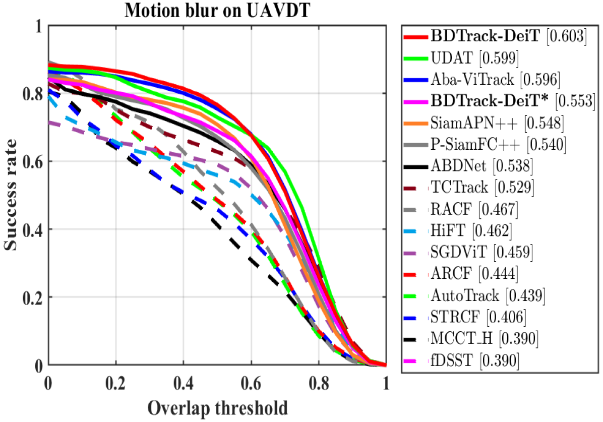
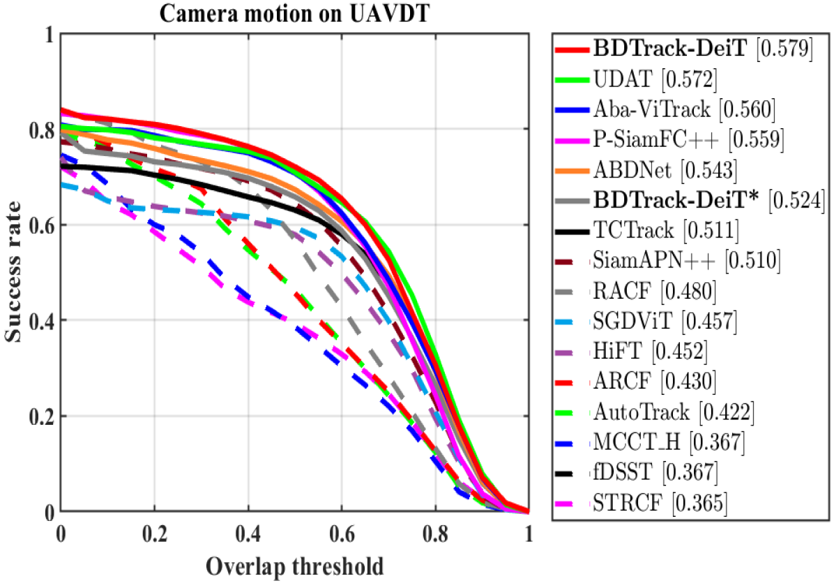
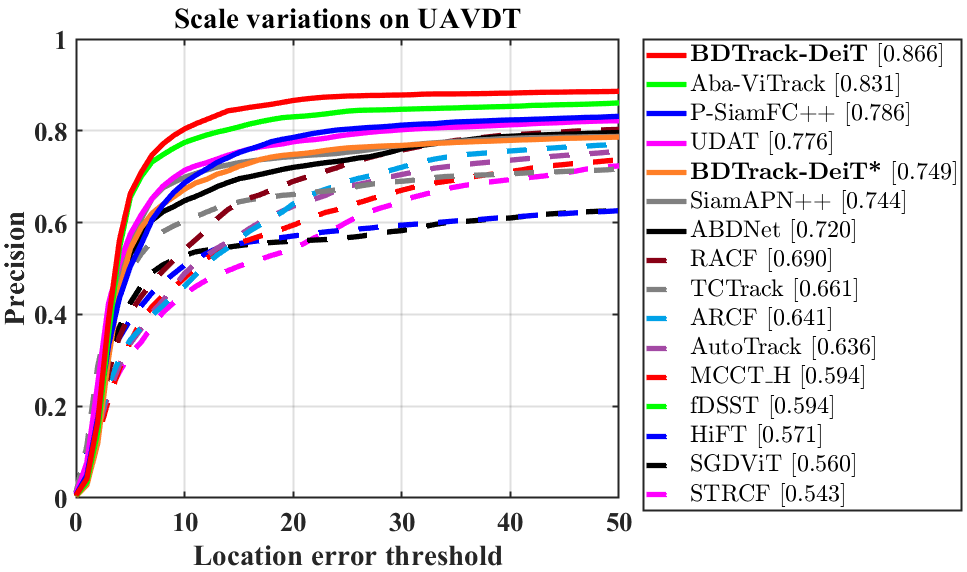
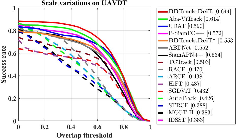
Figure 4: The precision plots and success plots of attribute-based comparison are presented for the attribute subsets of UAVDT. Note that BDTrack-DeiT* denotes BDTrack-DeiT without the application of the proposed components.

IV-C Attribute-Based Evaluation

To further validate the superiority of the proposed tracker over existing UAV trackers, we assess the performance of BDTrack-DeiT by comparing it with 14 SOTA UAV trackers on three subsets of the UAVDT dataset, including ‘Motion blur’, ‘Camera motion’, and ‘Scale variations’. Note that we also evaluate BDTrack-DeiT without applying the components (i.e., MBRV and DEEM), denoted as BDTrack-DeiT* for reference. The precision and success plots are illustrated in Fig. 4. As observed, BDTrack-DeiT significantly outperforms the second tracker on ‘Motion blur’, ‘Camera motion’ and ‘Scale variations’, with gains of 1.2%/0.4%, 2.1%/0.7%, and 3.5%/3.0% in precision/success rate, respectively. Significantly, across all these three attributes, the incorporation of the proposed components yields a noteworthy enhancement over BDTrack-DeiT*, with improvements of 7.0%/5.0%, 7.9%/5.5%, and 11.7%/9.1% in terms of precision and success rate. Note that ”Camera motion” and ”Scale variations” are both factors that can contribute to motion blur in visual tracking systems. When a camera moves rapidly or changes direction suddenly, it can cause motion blur in the captured images. While scale variations themselves do not directly cause motion blur, they can complicate the tracking process. If an object moves quickly closer or farther away and the camera or algorithm doesn’t adjust well, the object can appear blurred in the images. This happens because the object’s speed relative to the camera’s frame rate and exposure time changes, which can result in motion blur. Therefore, this attribute-based evaluation validates, directly or indirectly, the superiority and effectiveness of the proposed method in addressing the challenges posed by motion blur.

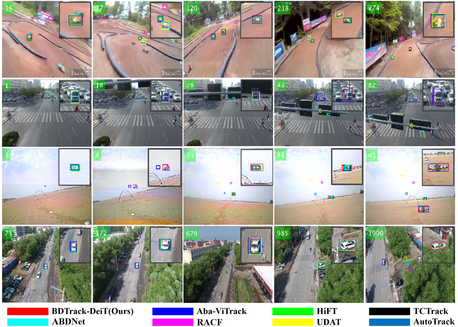
Figure 5: Qualitative evaluation on 4 video sequences from DTB70, UAVDT, UAV123@10fps, and VisDrone2018 (i.e. RcCar7, S0601, uav2, and uav0000208_00000_s), respectively.

IV-D Qualitative evaluation

Qualitative tracking results of BDTrack-DeiT and seven SOTA trackers, i.e., Aba-ViTrack [18], HiFT [1], TCTrack [5], ABDNet [33], RACF [6], UDAT [55], and AutoTrack [11], are presented in Fig. 5. Four video sequences from four different benchmarks are selected for demonstration: RcCar7 from DTB70, S0601 from UAVDT, uav2 from UAV123@10fps, and uav0000208_00000_s from VisDrone2018. For better visualization, the low-resolution targets within the video frames are selectively zoomed, cropped, and placed in the upper right corner of their corresponding frames for display. Notably, only our tracker successfully tracks the targets in all challenging examples, featuring motion blur (i.e, RcCar7 and uav2), occlusion (i.e, S0601 and uav0000208_00000_), low resolution (i.e, uav2), and scale variations (i.e, in all sequences). Specifically, BDTrack-DeiT is the only tracker to successfully track the target in uav0000208_00000_s. In S0601, while Aba-ViTrack, RACF, AutoTrack, and BDTrack-DeiT all successfully track the target, BDTrack-DeiT demonstrates higher accuracy. In the remaining sequences, BDTrack-DeiT consistently proves to be the most accurate tracker. Our method not only exhibits superior performance but also delivers more visually pleasing results in these scenarios, further validating the effectiveness of the proposed method for UAV tracking.

IV-E Comparison with Deep Trackers

The proposed BDTrack-DeiT is also compared with 12 SOTA deep trackers, i.e., PrDiMP50 [79], AutoMatch [77], SOAT [78], CSWinTT [76], SimTrack[14], OSTrack [13], ZoomTrack [15], SeqTrack [70], MAT [74], SuperSBT [71], DCPT [73], and EVPTrack [72]. We utilize Table II to present the results of precision (Prec.) and success rate (Succ.), their average (Avg.), and average GPU Speed (Avg.FPS). Our BDTrack-DeiT stands out by offering the fastest speed without compromising on high performance, showcasing its competitive edge in terms of both performance and speed. Remarkably, our method achieves second place in both Avg. precision on five benchmarks and precision on UAVDT, while securing the top position in precision on VisDrone2018. This underscores the effectiveness of our approach for UAV tracking tasks and highlights that our BDTrack-DeiT is equivalent in precision to state-of-the-art deep trackers. Although other deep trackers like SeqTrack [70] and EVPTrack [72] may achieve comparable performance with ours, their GPU speeds are significantly slower. In fact, our method outperforms SeqTrack and EVPTrack by being 9 and 11 times faster, respectively. By showcasing its capability to offer high precision and speed, these results demonstrate the suitability of our approach for real-time UAV tracking applications that prioritize accuracy and efficiency.

TABLE II: Precision (Prec.), success rate (Succ.), and GPU speed comparison between BDTrack-DeiT and DL-based trackers.

		DTB70		UAVDT		VisDrone2018		UAV123		UAV123@10fps		Avg.
Tracker	Source	Prec.	Succ.	Prec.	Succ.	Prec.	Succ.	Prec.	Succ.	Prec.	Succ.	Prec.	Succ.	Avg.FPS
PrDiMP50[79]	CVPR 20	84.0	64.3	75.8	55.9	79.8	60.2	87.2	66.5	83.9	64.7	82.1	62.3	53.6
AutoMatch[77]	ICCV 21	82.5	63.4	82.1	60.8	78.1	59.6	83.8	64.4	78.1	59.4	80.9	61.9	63.9
SOAT[78]	ICCV 21	83.1	64.6	82.1	60.7	76.9	59.1	82.7	64.9	85.2	65.7	82.0	63.0	36.2
CSWinTT[76]	CVPR 22	80.3	62.3	67.3	54.0	75.2	58.0	87.6	70.5	87.1	68.1	79.5	62.6	12.3
SimTrack[14]	ECCV 22	83.2	64.6	76.5	57.2	80.0	60.9	88.2	69.2	87.5	69.0	83.1	64.2	72.8
OSTrack[13]	ECCV 22	82.7	65.0	85.1	63.4	84.2	64.8	84.7	67.4	83.1	66.1	83.9	65.3	68.4
ZoomTrack[15]	NIPS 23	82.0	63.2	77.1	57.9	81.4	63.6	88.4	69.6	88.8	70.0	83.5	64.8	62.7
SeqTrack[70]	CVPR 23	85.6	65.5	78.7	58.8	83.3	64.1	86.8	68.6	85.7	68.1	84.0	65.0	32.3
MAT[74]	CVPR 23	83.2	64.5	72.9	54.8	81.6	62.2	86.7	68.3	86.9	68.5	82.3	63.6	71.2
SuperSBT[71]	arXiv’24	84.4	65.1	80.1	59.2	82.2	63.5	85.3	67.3	87.3	69.1	83.9	64.8	32.5
DCPT[73]	ICRA 24	84.0	64.8	76.8	56.9	83.1	64.2	85.7	68.1	86.9	69.1	83.3	64.6	39.2
EVPTrack[72]	AAAI 24	85.8	66.5	80.6	61.2	84.5	65.8	88.9	70.2	88.7	70.4	85.7	66.8	26.1
BDTrack-DeiT	Ours	83.5	64.1	84.1	61.0	85.2	64.3	84.8	66.7	83.5	65.9	84.2	64.4	287.2

TABLE III: Comparison of FLOPS, parameters, and inference speed on NVIDIA Jetson AGX Xavier edge device (AGX.FPS) with ten efficient lightweight trackers, evaluated on UAVDT.

Tracker	Source	FLOPs	Params.	AGX.FPS
BDTrack-DeiT		1.7G-2.4G	5.8M-8.0M	44.9
BDTrack-ViT		1.7G-2.4G	5.8M-8.0M	40.9
BDTrack-T2T	Ours	1.9G-2.4G	5.4M-7.0M	40.1
LightFC [54]	KBS 24	2.9G	7.5M	34.7
SMAT [53]	WACV 24	3.2G	8.6M	33.8
Aba-ViTrack [18]	ICCV 23	2.4G	8.0M	37.3
HiT [51]	ICCV 23	1.3G	11.0M	41.2
ABDNet [33]	RAL 23	8.27G	12.3M	33.2
SGDViT [56]	ICRA 23	11.3G	23.3M	32.1
DRCI [57]	ICME 23	3.6G	8.8M	44.6
TCTrack [5]	CVPR 22	6.9G	8.5M	34.4
HCAT [58]	ECCV 22	2.6G	8.4M	34.8
HiFT [1]	ICCV 21	7.2G	9.9M	35.6

TABLE IV: Ablation study of the impact of MBRV and DEEM on the baseline trackers’ performance on DTB70, UAVDT, VisDrone2018, UAV123, and UAV123@10fps. Note that precision and success rate are shown in the form of (Prec. , Succ.)

Tracker	MBRV	DEEM	DTB70	UAVDT	VisDrone2018	UAV123	UAV123@10fps	Avg.	Avg.FPS
			(79.3, 62.4)	(77.0, 55.6)	(83.0, 62.7)	(83.2, 66.5)	(82.1, 64.8)	(80.9, 62.4)	195.4
	$\checkmark$		(83.5, 64.7)	(79.3, 57.4)	(84.6, 63.8)	(84.7, 66.9)	(84.5, 66.4)	(83.3↑2.4, 63.8↑1.4)	-
BDTrack-ViT	$\checkmark$	$\checkmark$	(82.8, 64.2)	(78.9, 57.3)	(83.9, 63.6)	(83.5, 65.5)	(84.1, 66.1)	(82.6↑1.7, 63.3↑0.9)	238.6↑22%
			(78.6, 62.0)	(73.5, 53.7)	(81.2, 62.1)	(81.9, 64.9)	(79.2. 63.2)	(78.9, 61.2)	202.1
	$\checkmark$		(81.6, 63.6)	(78.5, 56.8)	(82.8, 63.1)	(81.5, 64.3)	(83.3, 65.3)	(81.5↑2.6, 62.6↑1.4)	-
DBTrack-T2T	$\checkmark$	$\checkmark$	(80.7, 63.0)	(77.9, 56.3)	(81.4, 62.2)	(80.4, 63.4)	(82.9, 65.1)	(80.6, 62.0)	240.4↑19%
			(84.2, 65.1)	(78.6, 56.7)	(81.6, 62.2)	(83.7, 66.1)	(82.7, 65.6)	(82.2, 63.2)	232.5
	$\checkmark$		(84.9, 65.6)	(84.5, 61.4)	(86.1, 65.1)	(85.3, 67.0)	(84.2, 66.2)	(84.8↑2.6, 65.0↑1.8)	-
DBTrack-DeiT	$\checkmark$	$\checkmark$	(83.5, 64.1)	(84.1, 61.0)	(85.2, 64.3)	(84.8, 66.7)	(83.5, 65.9)	(84.2↑2.0, 64.4↑1.2)	287.2↑24%

IV-F Efficiency Comparison

To highlight the superiority of the proposed trackers over existing ones in terms of efficiency, we present in Table III the floating-point operations per second (FLOPs), the number of parameters during inference (Param.), and the speed on the Nvidia Jetson AGX Xavier edge device (AGX.FPS) of our method and 10 state-of-the-art efficient lightweight trackers. Notably, as our methods feature adaptive architectures, the FLOPs and Params. of our method vary within a range, spanning from the minimum to the maximum values. As observed, our methods achieve significantly lower FLOPs and Params. compared to all rival trackers, except for HiT, which secures the lowest FLOPs. Even our maximum values are lower than those of most trackers. Although HiT has the lowest FLOPs, its Params. is significantly larger than ours, and its tracking performance across multiple UAV tracking benchmarks is notably inferior, as shown in Table I. In terms of AGX speed, our BDTrack-DeiT attains the highest speed of 44.9 FPS. Additionally, our BDTrack-ViT and BDTrack-T2T, with speeds exceeding 40 FPS, also surpass most rival trackers.

IV-G Ablation Study

IV-G1 Impact of learning blur robust ViTs with dynamic early exit

We add the proposed components MBRV and DEEM into the baselines one by one to evaluate their effectiveness. The evaluation results on five benchmarks are shown in Table IV. As GPU speed of the baseline and its enhanced version by MBRV are theoretically equal, we provide only the speed of the baseline to eliminate potential nuances arising from randomness. As can be seen, the inclusion of MBRV leads to significant improvements in both Prec. and Succ. for all baseline trackers. Specifically, the inclusion of the MBRV leads to a significant increase of over 2.0% in average Prec. and 1.0% in average Succ. for all baseline trackers. When DEEM is further integrated, consistent improvements in GPU speeds are observed, accompanied by only slight decreases in Prec. and Succ. Specifically, the GPU speeds of all baselines see increases of above 19.0%, with BDTrack-DeiT achieving a remarkable 24.0% improvement. Despite the marginal drop in Prec. and Succ. (the average drops are less than 0.9%), the overall pattern of enhanced GPU speeds and minor sacrifices in tracking performance validates the effectiveness of DEEM in optimizing tracking efficiency.

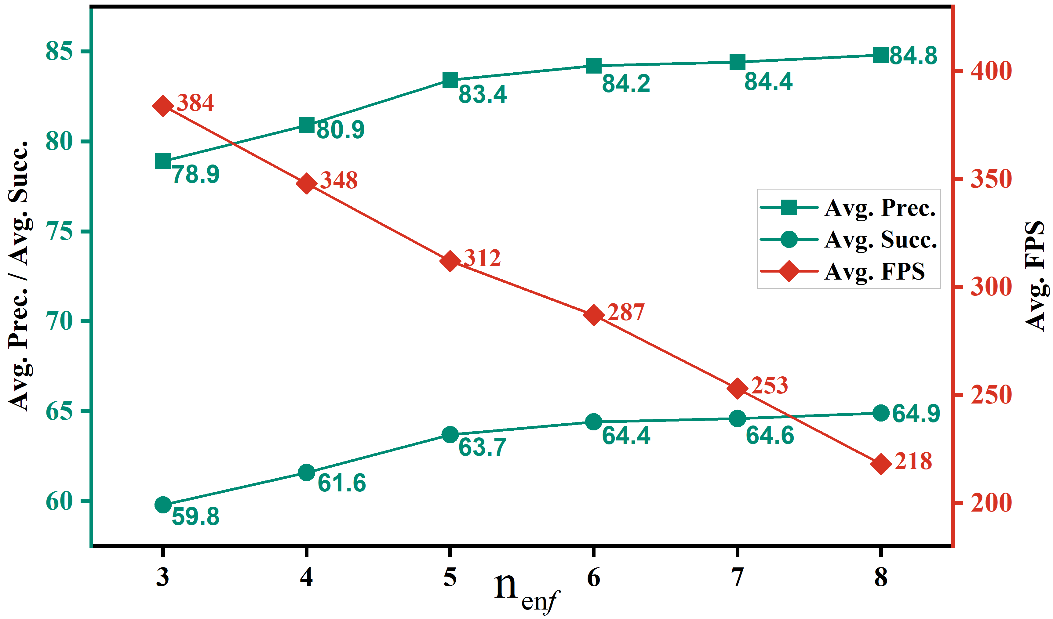
Figure 6: Ablation study on when to initiate the DEEM. The figure presents the results for average precision (Avg. Prec.), average success rate (Avg. Succ.), and average tracking GPU speed (Avg. FPS) with respect to $n_{enf}$ across the five datasets.

IV-G2 Study on when to initiate the DEEM

We conducted experiments to examine the impact of the timing of initiating the DEEM on performance by varying the parameter $n_{enf}$ from 3 to 8. Fig. 6 presents the results of average precision (Avg. Prec.), average success rate (Avg. Succ.), and average GPU speed (Avg. FPS) across the five datasets. As shown, the timing of initializing the DEEM in BDTrack-DeiT directly impacts both the tracking performance and speed. Specifically, increasing $n_{enf}$ results in an upward trend for both Avg. Prec. and Avg. Succ., but a decrease in Avg. FPS. When $n_{enf}$ falls in the range of 3 to 5, each additional layer leads to about 2.0% increase in both Avg. Prec. and Avg. Succ., while causing about 10% drop in speed. When the value of $n_{enf}$ exceeds 6, further increases in $n_{enf}$ do not result in significant improvements in precision and success rate, while the speed continues to gradually decrease significantly. Considering the trade-off between performance and speed, we have chosen to set the default value of $n_{enf}$ as 6 in our implementation.

TABLE V: Ablation study on the weighting of loss $\mathcal{L}_{br}$ in training BDTrack-DeiT by varying $\rho$ from $0.5\times 10^{-4}$ to $5.0\times 10^{-4}$. Note that precision and success rate are shown in the form of (Prec. , Succ.).

$\rho\times 10^{-4}$	DTB70	UAVDT	VisDrone2018	UAV123	UAV123@10fps	Avg.
0.5	(82.2, 63.6)	(83.4, 60.0)	(83.7, 63.5)	(83.1, 65.4)	(83.2, 65.6)	(83.1, 63.6)
$0.6$	(82.9, 63.9)	(82.3, 59.3)	(84.5, 63.9)	(83.7, 66.0)	(83.0, 65.4)	(83.3, 63.7)
$0.7$	(83.2, 63.8)	(83.0, 59.6)	(85.8, 64.6)	(84.1, 66.5)	(83.3, 66.2)	(83.9, 64.1)
$0.8$	(84.5, 64.8)	(83.2, 59.8)	(81.1, 61.9)	(83.5, 65.8)	(82.3, 64.9)	(82.9, 63.4)
$0.9$	(81.8, 62.9)	(82.5, 59.7)	(84.6, 63.9)	(84.0, 66.1)	(83.1, 65.6)	(83.2, 63.6)
$1.0$	(83.5, 64.1)	(84.1, 61.0)	(85.2, 64.3)	(84.8, 66.7)	(83.5, 65.9)	(84.2, 64.4)
$2.0$	(83.2, 64.5)	(80.4, 58.2)	(86.1, 64.8)	(84.0, 65.9)	(84.9, 66.5)	(83.7, 64.0)
$3.0$	(83.4, 64.3)	(83.8, 60.7)	(85.6, 64.5)	(82.4, 64.7)	(80.2, 63.6)	(83.1, 63.6)
$4.0$	(81.6, 62.8)	(82.4, 59.4)	(84.5, 63.8)	(84.5, 66.5)	(80.0, 63.5)	(82.6, 63.2)
$5.0$	(84.1, 64.6)	(82.6, 59.7)	(83.9, 63.6)	(84.0, 66.0)	(82.3, 65.1)	(83.4, 63.8)

TABLE VI: Ablation study on the weighting of loss $\mathcal{L}_{spar}$ in training BDTrack-DeiT by varying $\gamma$ from $0.5\times 10^{3}$ to $1.5\times 10^{3}$. Note that precision and success rate are shown in the form of (Prec. , Succ.).

$\gamma\times 10^{3}$	DTB70	UAVDT	VisDrone2018	UAV123	UAV123@10fps	Avg.
$0.5$	(84.1, 65.0)	(81.2, 58.6)	(83.7, 63.1)	(83.4, 65.6)	(81.5, 64.8)	(82.8, 63.5)
$0.6$	(82.5, 64.4)	(81.1, 58.7)	(86.7, 65.3)	( 84.1, 66.0)	(82.3, 65.2)	(83.3, 63.9)
$0.7$	(82.9, 64.4)	(81.9, 59.0)	(83.9, 63.7)	(82.9, 65.2)	(83.4, 65.7)	(83.0, 63.6)
$0.8$	( 83.7, 64.9)	(84.2, 60.4)	(83.2, 63.0)	(83.6, 65.6)	(82.7, 65.2)	(83.5, 63.8)
$0.9$	(82.7, 64.2)	( 84.0, 60.7)	( 86.2, 64.9)	(82.9, 65.3)	(83.0, 65.4)	( 83.8, 64.1)
$1.0$	(83.5, 64.1)	(84.1, 61.0)	(85.2, 64.3)	(84.8, 66.7)	( 83.5, 65.9)	(84.2, 64.4)
$1.1$	(81.6, 63.9)	(83.5, 60.2)	(84.7, 64.2)	(83.4, 65.6)	(83.0, 65.4)	(83.3, 63.8)
$1.2$	(84.3, 65.1)	(82.7, 59.8)	(83.6, 63.2)	(84.5, 66.2)	(84.9, 66.5)	(84.0, 64.2)
$1.3$	(83.1, 63.7)	(82.7, 59.7)	(84.6, 63.6)	(83.8, 65.9)	(84.1, 64.1)	(83.7, 63.5)
$1.4$	(81.0, 61.9)	(82.5, 59.9)	(87.6, 66.1)	(84.0, 65.9)	(82.4, 63.5)	(83.5, 63.4)
$1.5$	(81.2, 62.0)	(83.9, 60.5)	(83.7, 63.4)	(82.7, 65.4)	(81.7, 64.3)	(82.7, 63.0)

IV-G3 Study on weighting the loss for learning motion blur robust ViTs (MBRV)

To observe how the weight $\rho$ of the loss $\mathcal{L}_{br}$ influence the performance, we train BDTrack-DeiT with various $\rho$ values ranging from $0.5\times 10^{-4}$ to $5.0\times 10^{-4}$. The evaluation results assessed across all five datasets are shown in Table V. Obviously, BDTrack-DeiT achieves averagely the optimal performance at $\rho$ = $1.0\times 10^{-4}$, with 84.2% Avg. Prec. and 64.4% Avg. Succ.. Additionally, we can observe that the second and third-best performances across these datasets are scattered both above and below the value of $1.0\times 10^{-4}$. These fluctuations may be attributed to the inherent differences between these datasets. When $\rho$ is set as $4.0\times 10^{-4}$, BDTrack-DeiT achieves the lowest average performance, with 82.6% Avg. Prec. and 63.2% Avg. Succ. This indicates that selecting an appropriate weight $\rho$ is crucial for achieving optimal tracking performance. An ill-suited $\rho$ can adversely affect the training process, leading to suboptimal results. The performance variations observed with different $\rho$ values highlight the sensitivity of the tracking algorithm to this parameter. Therefore, careful tuning of $\rho$ is necessary to ensure that the model performs effectively across diverse datasets and scenarios.

IV-G4 Study on weighting the proposed block sparsity loss

In order to provide a detailed analysis of the impact of the proposed block sparsity loss $\mathcal{L}_{spar}$ on the performance, Table VI presents the evaluation results of BDTrack-DeiT trained with various block sparsity loss weight $\gamma$ values ranging from $0.5\times 10^{3}$ to $1.5\times 10^{3}$. Note that during training, the weight $\rho$ of the loss $\mathcal{L}_{br}$ is set to $1.0\times 10^{-4}$. As shown in the table, BDTrack-DeiT achieves the optimal performance when the $\gamma$ is set to $1.0\times 10^{3}$. When $\gamma$ is increased to $1.5\times 10^{3}$, BDTrack-DeiT shows a significant drop, achieving the lowest average performance with a 1.5% decrease in Avg. Prec. and a 1.4% decrease in Avg. Succ. The experimental results demonstrate that the choice of weight $\gamma$ significantly impacts tracking performance, and improper selection of this parameter can lead to suboptimal performance.

IV-G5 Application to SOTA trackers

To demonstrate the general applicability of our approach, we integrate the proposed MBRV and DEEM into three SOTA trackers: ARTrack [80], GRM [69], and DropTrack [81]. Note that we substitute their original backbones with the tiny ViT, i.e., ViT-Tiny [65], to save training time. The evaluation results on five benchmarks are presented in Table VII. As mentioned previously, we provide only the speed of the baseline to eliminate potential nuances arising from randomness. We can observe that the inclusion of MBRV leads to noticeable improvements in both Prec. and Succ. for all baselines. Specifically, ARTrack, GRM, and DropTrack experience increases of 1.8%, 1.3%, and 1.7% in Avg. Prec., respectively, while their Avg. Succ. grows by 1.3%, 1.0%, and 1.1%, respectively. When DEEM is further integrated, we consistently observe improvements in GPU speeds, along with only slight decreases in Prec. and Succ. More specifically, the GPU speeds of all baselines demonstrate increases of more than 14.0%, with tracking performance dropping by less than 0.6%. These results confirm the applicability of our method in enhancing the efficiency of existing ViT-based trackers without significantly compromising tracking performance, justifying its generality.

TABLE VII: Application of our MBRV and DEEM to SOTA trackers. Note that precision and success rate are shown in the form of (Prec., Succ.)

Tracker	MBRV	DEEM	DTB70	UAVDT	VisDrone2018	UAV123	UAV123@10fps	Avg.	Avg.FPS
ARTrack[80]			(79.6, 61.2)	(74.7, 52.8)	(78.6, 60.1)	(80.4, 63.1)	(80.1, 63.3)	(78.6, 60.1)	78.3
	$\checkmark$		(80.1, 62.0)	(76.7, 54.7)	(79.8, 60.6)	(81.6, 63.9)	(83.9, 66.0)	(80.4↑1.8, 61.4↑1.3)	-
	$\checkmark$	$\checkmark$	(79.2, 61.5)	(76.0, 54.1)	(79.4, 60.3)	(80.9, 63.6)	(83.4, 65.7)	(79.8↑1.2, 61.0↑0.9)	89.3↑14%
GRM [69]			(81.8, 63.6)	(78.1, 56.9)	(85.5, 64.8)	(84.6, 66.5)	(82.6, 65.3)	(82.5, 63.4)	224.3
	$\checkmark$		(83.1, 65.2)	(80.4, 58.4)	(86.2, 65.3)	(85.4, 67.1)	(84.0, 66.0)	(83.8↑1.3, 64.4↑1.0)	-
	$\checkmark$	$\checkmark$	(82.9, 64.9)	(79.9, 58.1)	(85.5, 64.8)	(85.0, 66.8)	(83.5, 65.7)	(83.4↑0.9, 64.1↑0.7)	261.1↑16%
DropTrack [81]			(83.4, 64.7)	(79.4, 57.5)	(81.9, 61.8)	(84.8, 66.2)	(82.5, 65.1)	(82.4, 63.1)	214.6
	$\checkmark$		(84.2, 65.3)	(81.6, 58.9)	(85.1, 64.2)	(85.4, 66.6)	(84.0, 66.1)	(84.1↑1.7, 64.2↑1.1)	-
	$\checkmark$	$\checkmark$	(83.5, 64.9)	(81.0, 58.4)	(84.7, 64.3)	(85.0, 66.3)	(83.7, 65.8)	(83.6↑1.2, 63.9↑0.8)	253.8↑18%

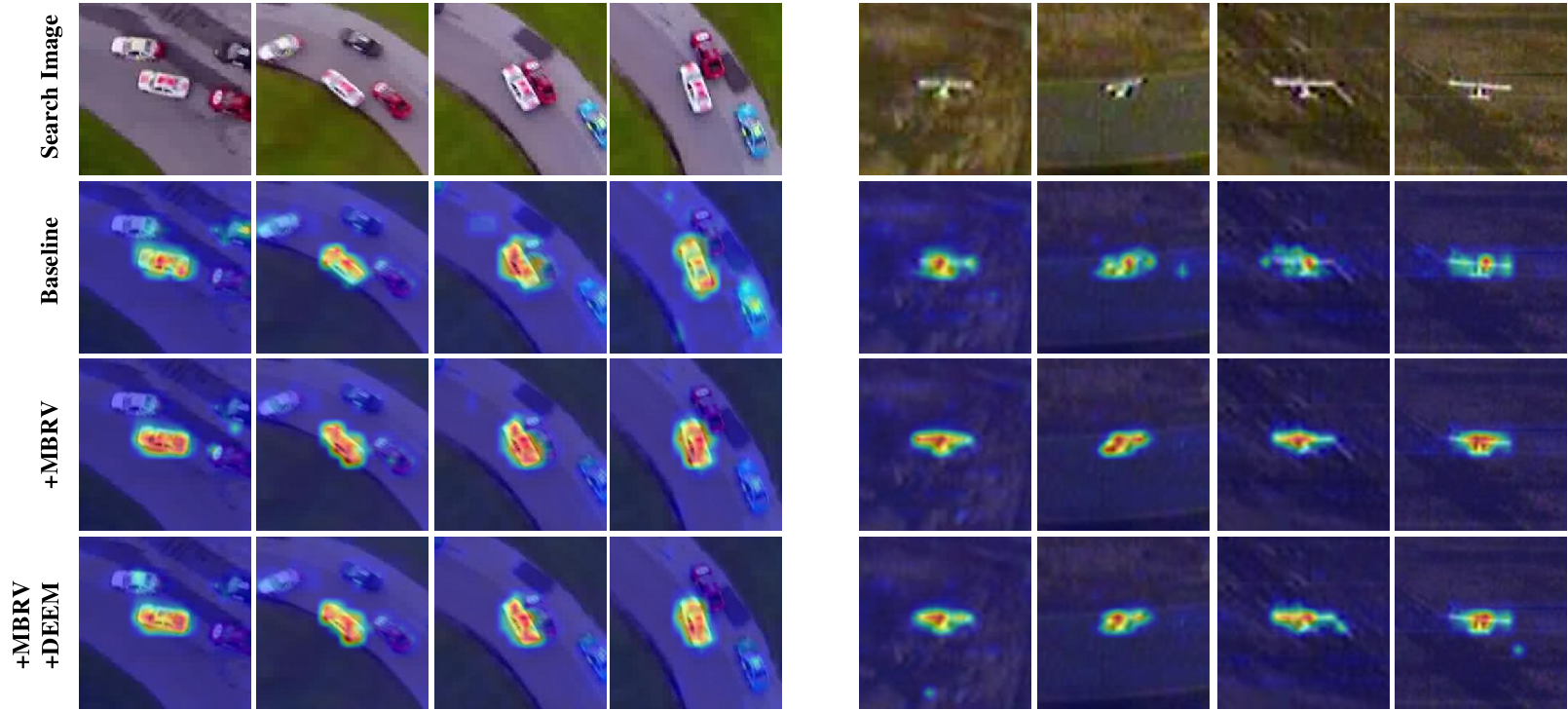
Figure 7: Visualization of attention maps. The first row displays the original search images, while the second, third, and fourth rows showcase the attention maps generated by BDTrack-DeiT without and with incorporating the proposed components.

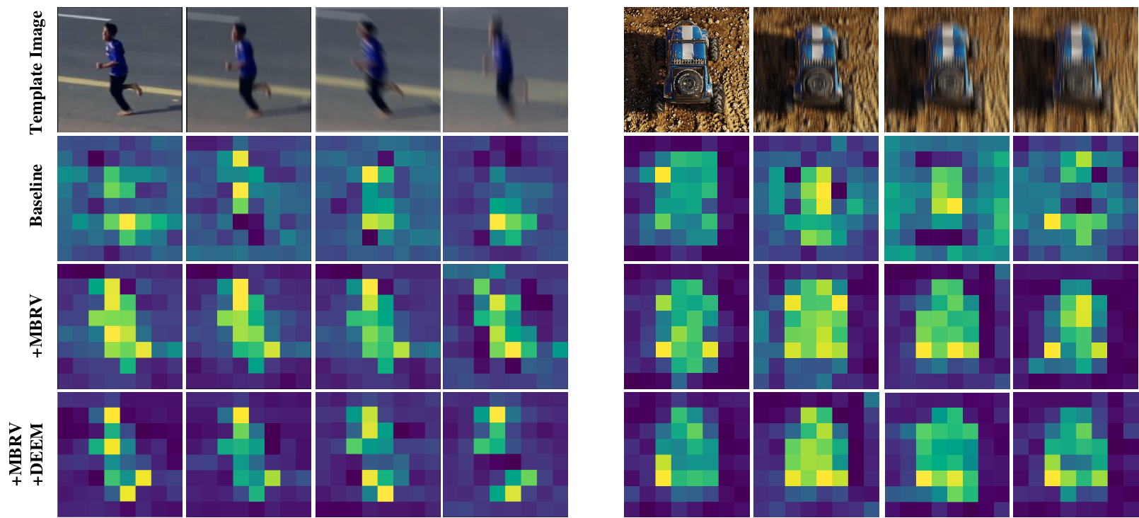
Figure 8: Visualization of feature maps. For each group, we present the original template images and their blurred versions (top row), followed by the feature maps generated by BDTrack-DeiT without (second row) and with (third and fourth rows) the proposed components. The the kernel size for linear motion blur is 3, 5 , 7, from left to right.

IV-G6 Qualitative Results

Our BDTrack enhances the robustness of Vision Transformers (ViTs) against motion blur by enforcing invariance in the feature representation of the target. To intuitively demonstrate the effectiveness of the proposed components, Fig. 7 and Fig. 8 visualize several example attention maps of the search images and example feature maps of the template images generated by BDTrack with and without the proposed components (i.e., MBRV and DEEM). Note that in these examples the targets are subjected to motion blur. For convenience, a ’*’ suffix is added to BDTrack-DeiT to denote the baseline that excludes any of the proposed components. A ’+’ suffix indicates the inclusion of the MBRV component in the baseline, while a ’++’ suffix signifies the incorporation of both the MBRV and DEEM components into the baseline.

Example attention maps of the search images. In Fig. 7, the first row shows the original search images from two example sequences (i.e., SpeedCar4 and uav1), one from DTB70 [64] and the other from UAV123 [61]. The images in the second, third, and fourth rows are the corresponding attention maps generated by BDTrack-DeiT*, BDTrack-DeiT+, and BDTrack-DeiT++ (i.e., BDTrack-DeiT), respectively. As can be seen, incorporating the MBRV component (i.e., BDTrack-DeiT+) and both the MBRV and DEEM components (i.e., BDTrack-DeiT++) yields very similar results. Specifically, their visual focus on the targets is more pronounced compared to the baseline tracker (i.e., BDTrack-DeiT*). This demonstrates that the MBRV component is able to enhance the tracker’s ability to concentrate on the target, especially under motion blur conditions, thereby improving overall tracking performance.

Example feature maps of the template images. In each group of Fig. 8, the first row displays the original template and its blurred versions using the linear motion blur method [43] with kernel sizes 3, 5, 7 from left to right, respectively. The corresponding feature maps produced by BDTrack-DeiT*, BDTrack-DeiT+, and BDTrack-DeiT++ are shown in the second, third, and fourth rows, respectively. This comparison provides a visual representation of the impact of the proposed MBRV and DEEM components. As can be seen, the feature maps generated by BDTrack-DeiT+ and BDTrack-DeiT++ show more consistency with changes in kernel size, whereas the feature maps from BDTrack-DeiT* display more significant variations, especially at larger kernel sizes. These qualitative results provide visual evidence for the effectiveness of our method in learning motion blur robust feature representations with ViTs.

Figure 9: Real-world test on an embedded device. The CLE plots illustrate the frame-wise performance, where errors below a CLE of 20 pixels are usually considered acceptable. Note that the ground truth and tracking results are denoted by red and green boxes, respectively.

IV-H Real-World Test

To evaluate our method’s tracking performance under real-world conditions, we conducted tests on the NVIDIA Jetson AGX Xavier 32GB, a platform well-suited for UAV applications due to its compactness and computational efficiency. We used the UAVTrack112_L dataset [75] to evaluate our BDTrack-DeiT, which cover a variety of UAV scenes. Fig. 9 showcases two diverse real-world scenarios where the objects are subjected to motion blur, low resolution, fast motion challenges among others. As can be seen, our BDTrack-DeiT demonstrates robust and satisfactory performance under these challenging real-world conditions. Specifically, it maintains a Center Location Error (CLE) of fewer than 20 pixels in all test frames, indicating high precision in tracking. Furthermore, BDTrack-DeiT consistently achieves real-time average speeds of 44 FPS. These results highlight our tracker’s robustness and efficiency, making it well-suited for UAV applications that demand high performance and speed.

V Conclusions

In this work, our focus was on exploring efficient and motion blur robust Vision Transformers (ViTs) within a unified framework for real-time UAV tracking. We achieved this by tailoring the framework into an adaptive computation paradigm that dynamically early exits Transformer blocks. Moreover, in addressing the prevalent challenges associated with motion blur in UAV tracking, our approach focuses on learning motion blur robust Vision Transformers (ViTs). This is achieved by enforcing invariance in the feature representation of the target against simulated motion blur. Remarkably, our method stands out for its simplicity, making it easily integrable or adaptable into other tracking frameworks without necessitating additional architectures. Extensive experiments across five challenging UAV benchmarks were conducted to validate the effectiveness of our proposed method. The experimental results demonstrate that our BDTrack-DeiT achieves state-of-the-art performance in real-time UAV tracking.

References

- [1] Z. Cao, C. Fu, and et al, “Hift: Hierarchical feature transformer for aerial tracking,” in ICCV, 2021, pp. 15 457–15 466.
- [2] S. Li, X. Yang, and et al, “Learning Target-Aware Vision Transformers for Real-Time UAV Tracking,” IEEE TGRS, 2024.
- [3] F. Lin, C. Fu, and et al, “Learning temporary block-based bidirectional incongruity-aware correlation filters for efficient uav object tracking,” IEEE TCSVT, vol. 31, no. 6, pp. 2160–2174, 2020.
- [4] X. Liu, T. Xu, and et al, “Bactrack: Building appearance collection for aerial tracking,” IEEE TCSVT, vol. 34, pp. 5002-5017, 2023.
- [5] Z. Cao, Z. Huang, and et al, “Tctrack: Temporal contexts for aerial tracking,” in CVPR, 2022, pp. 14 798–14 808.
- [6] S. Li, Y. Liu, and et al, “Learning residue-aware correlation filters and refining scale for real-time uav tracking,” PR, vol. 127, p. 108614, 2022.
- [7] J. F. Henriques, R. Caseiro, and et al, “High-speed tracking with kernelized correlation filters,” TPAMI, vol. 37, no. 3, pp. 583–596, 2015.
- [8] C. Tang, X. Wang, and et al, “Learning spatial-frequency transformer for visual object tracking,” IEEE TCSVT, vol. 33, no. 9, pp. 5102–5116, 2023.
- [9] Z. Huang, C. Fu, Y. Li, F. Lin, and P. Lu, “Learning aberrance repressed correlation filters for real-time uav tracking,” in ICCV, pp. 2891–2900, 2019.
- [10] J. Ding, Y. Huang, and et al, “Severely blurred object tracking by learning deep image representations,” IEEE TCSVT, vol. 26, no. 2, pp. 319–331, 2015.
- [11] Y. Li, C. Fu, and et al, “Autotrack: Towards high-performance visual tracking for uav with automatic spatio-temporal regularization,” in CVPR, 2020, pp. 11 923–11 932.
- [12] X. Yuan, T. Xu, and et al, “Multi-step temporal modeling for uav tracking,” IEEE TCSVT, 2024.
- [13] B. Ye, H. Chang, and et al, “Joint feature learning and relation modeling for tracking: A one-stream framework,” in ECCV. Springer, 2022, pp. 341–357.
- [14] B. Chen, P. Li, and et ali, “Backbone is all your need: A simplified architecture for visual object tracking,” in ECCV. Springer, 2022, pp. 375–392.
- [15] Y. Kou, J. Gao, B. Li, G. Wang, W. Hu, Y. Wang, and L. Li, “Zoomtrack: Target-aware non-uniform resizing for efficient visual tracking,” NIPS, vol. 36, 2023.
- [16] L. Yang, S. Gu, and et al, “Skeleton neural networks via low-rank guided filter pruning,” IEEE TCSVT, vol. 33, pp. 7197–7211, 2023.
- [17] F. Xie, C. Wang, and et al, “Correlation-aware deep tracking,” in CVPR, 2022, pp. 8751–8760.
- [18] S. Li, Y. Yang, and et al, “Adaptive and background-aware vision transformer for real-time uav tracking,” in ICCV, 2023, pp. 13 989–14 000.
- [19] Y. Kaya, S. Hong, and et al, “Shallow-deep networks: Understanding and mitigating network overthinking,” in ICML, 2018.
- [20] H. Li, H. Zhang, and et al, “Improved techniques for training adaptive deep networks,” ICCV, pp. 1891–1900, 2019.
- [21] Y. Liu, F. Meng, and et al, “Faster depth-adaptive transformers,” in AAAI, 2020. [Online].
- [22] G. Xu, J. Hao, and et al, “Lgvit: Dynamic early exiting for accelerating vision transformer,” ACM MM, 2023.
- [23] M. Phuong and C. H. Lampert, “Distillation-based training for multi-exit architectures,” ICCV, pp. 1355–1364, 2019.
- [24] S. Teerapittayanon and et al, “Branchynet: Fast inference via early exiting from deep neural networks,” ICPR, pp. 2464–2469, 2016.
- [25] A. Ghodrati, B. E. Bejnordi, and et al, “Frameexit: Conditional early exiting for efficient video recognition,” CVPR, pp. 15 603–15 613, 2021.
- [26] Z. Fei, X. Yan, and et al, “Deecap: Dynamic early exiting for efficient image captioning,” CVPR, pp. 12 206–12 216, 2022.
- [27] S. Tang and et al, “You need multiple exiting: Dynamic early exiting for accelerating unified vision language model,” CVPR, pp. 10 781–10 791, 2022.
- [28] C. Fu, B. Li, and et al, “Correlation filters for unmanned aerial vehicle-based aerial tracking: A review and experimental evaluation,” IEEE GEOSC REM SEN M, vol. 10, pp. 125–160, 2020.
- [29] B. Ma, L. Huang, and et al, “Visual tracking under motion blur,” TIP, vol. 25, no. 12, pp. 5867–5876, 2016.
- [30] C. Seibold, A. Hilsmann, and et al, “Model-based motion blur estimation for the improvement of motion tracking,” CVIU, vol. 160, pp. 45–56, 2017.
- [31] Q. Guo, Z. Cheng, and et al, “Learning to adversarially blur visual object tracking,” in ICCV, 2021, pp. 10 839–10 848.
- [32] Q. Guo, W. Feng, and et al, “Effects of blur and deblurring to visual object tracking,” arXiv preprint arXiv:1908.07904, 2019.
- [33] H. Zuo, C. Fu, and et al, “Adversarial blur-deblur network for robust uav tracking,” RAL, vol. 8, no. 2, pp. 1101–1108, 2023.
- [34] Z. Mao, X. Chen, and et al, “Robust tracking for motion blur via context enhancement,” in ICIP. IEEE, 2021, pp. 659–663.
- [35] T. Askari, H. Hassanpour, and Javaran, “Retracted: Using a blur metric to estimate linear motion blur parameters,” 2023.
- [36] J. Mao, H. Yang, and et al, “Tprune: Efficient transformer pruning for mobile devices,” ACM Trans. Cyber Phys. Syst., vol. 5, pp. 26:1–26:22, 2021.
- [37] Y. Li, G. Yuan, and et al, “Efficientformer: Vision transformers at mobilenet speed,” ArXiv, vol. abs/2206.01191, 2022.
- [38] Y. Rao, W. Zhao, and et al, “Dynamicvit: Efficient vision transformers with dynamic token sparsification,” in NIPS, 2021.
- [39] H. Yin, Vahdat, and et al, “A-vit: Adaptive tokens for efficient vision transformer,” in CVPR, 2022, pp. 10 809–10 818.
- [40] J. Xin, R. Tang, and et al, “Berxit: Early exiting for bert with better fine-tuning and extension to regression,” in EACL, 2021.
- [41] J. Sivertsen, “Similarity problems in high dimensions,” ArXiv, vol. abs/1906.04842, 2019.
- [42] D. Srivamsi, O. M. Deepak, and et al, “Cosine similarity based word2vec model for biomedical data analysis,” ICOEI, pp. 1400–1404, 2023.
- [43] D. Dwibedi, I. Misra, and et al, “Cut, paste and learn: Surprisingly easy synthesis for instance detection,” ICCV, pp. 1310–1319, 2017.
- [44] H. Kiani Galoogahi, A. Fagg, and S. Lucey, “Learning background-aware correlation filters for visual tracking,” in ICCV, 2017, pp. 1135–1143.
- [45] M. Danelljan, G. Häger, and et al, “Discriminative scale space tracking,” TPAMI, vol. 39, no. 8, pp. 1561–1575, 2017.
- [46] M. Danelljan, G. Bhat, F. S. Khan, and M. Felsberg, “Eco: Efficient convolution operators for tracking,” CVPR, pp. 6931–6939, 2017.
- [47] N. Wang, W. Zhou, and et al, “Multi-cue correlation filters for robust visual tracking,” in CVPR, 2018, pp. 4844–4853.
- [48] F. Li, C. Tian, W. Zuo, L. Zhang, and M.-H. Yang, “Learning spatial-temporal regularized correlation filters for visual tracking,” in CVPR, 2018, pp. 4904–4913.
- [49] Z. Cao, C. Fu, J. Ye, B. Li, and Y. Li, “Siamapn++: Siamese attentional aggregation network for real-time uav tracking,” in IROS. IEEE, 2021, pp. 3086–3092.
- [50] B. Yan, H. Peng, K. Wu, D. Wang, J. Fu, and H. Lu, “Lighttrack: Finding lightweight neural networks for object tracking via one-shot architecture search,” CVPR, pp. 15 175–15 184, 2021.
- [51] B. Kang, X. Chen, D. Wang, H. Peng, and H. Lu, “Exploring lightweight hierarchical vision transformers for efficient visual tracking,” ICCV, pp. 9578–9587, 2023.
- [52] Q. Wei, B. Zeng, J. Liu, L. He, and G. Zeng, “Litetrack: Layer pruning with asynchronous feature extraction for lightweight and efficient visual tracking,” ArXiv, vol. abs/2309.09249, 2023.
- [53] G. Y. Gopal and M. A. Amer, “Separable self and mixed attention transformers for efficient object tracking,” in WACV, 2024, pp. 6708–6717.
- [54] Y. Li, B. Wang, X. Wu, Z. Liu, and Y. Li, “Lightweight full-convolutional siamese tracker,” Knowl. Based Syst., vol. 286, p. 111439, 2024.
- [55] J. Ye, C. Fu, and et al, “Unsupervised domain adaptation for nighttime aerial tracking,” in CVPR, 2022, pp. 8896–8905.
- [56] L. Yao, C. Fu, and et al, “Sgdvit: Saliency-guided dynamic vision transformer for uav tracking,” arXiv preprint arXiv:2303.04378, 2023.
- [57] D. Zeng, M. Zou, and et al, “Towards discriminative representations with contrastive instances for real-time uav tracking,” in ICME. IEEE, 2023, pp. 1349–1354.
- [58] X. Chen, B. Kang, D. Wang, D. Li, and H. Lu, “Efficient visual tracking via hierarchical cross-attention transformer,” in European Conference on Computer Vision. Springer, 2022, pp. 461–477.
- [59] H. Law and J. Deng, “Cornernet: Detecting objects as paired keypoints,” IJCV, vol. 128, pp. 642–656, 2018.
- [60] S. H. Rezatofighi, N. Tsoi, J. Gwak, A. Sadeghian, I. D. Reid, and S. Savarese, “Generalized intersection over union: A metric and a loss for bounding box regression,” CVPR, pp. 658–666, 2019.
- [61] M. Mueller, N. Smith, and et al, “A benchmark and simulator for uav tracking,” in ECCV. Springer, 2016, pp. 445–461.
- [62] L. Wen, P. Zhu, and et al, “Visdrone-sot2018: The vision meets drone single-object tracking challenge results,” in ECCV, 2018, pp. 0–0.
- [63] D. Du, Y. Qi, and et al, “The unmanned aerial vehicle benchmark: Object detection and tracking,” in ECCV, 2018, pp. 370–386.
- [64] S. Li and D.-Y. Yeung, “Visual object tracking for unmanned aerial vehicles: A benchmark and new motion models,” in AAAI, vol. 31, no. 1, 2017.
- [65] A. Dosovitskiy, L. Beyer, and et al, “An image is worth 16x16 words: Transformers for image recognition at scale,” arXiv preprint arXiv:2010.11929, 2020.
- [66] Touvron and et al, “Training data-efficient image transformers & distillation through attention,” in ICML. PMLR, 2021, pp. 10 347–10 357.
- [67] L. Yuan, Y. Chen, and et al, “Tokens-to-token vit: Training vision transformers from scratch on imagenet,” in ICCV, 2021, pp. 558–567.
- [68] Z. Zhang, H. Peng, and et al, “Ocean: Object-aware anchor-free tracking,” in ECCV. Springer, 2020, pp. 771–787.
- [69] S. Gao, C. Zhou, and et al, “Generalized relation modeling for transformer tracking,” in CVPR, 2023, pp. 18 686–18 695.
- [70] X. Chen, H. Peng, and et al, “Seqtrack: Sequence to sequence learning for visual object tracking,” in CVPR, 2023, pp. 14 572–14 581.
- [71] F. Xie, W. Yang, C. Wang, L. Chu, Y. Cao, C. Ma, and W. Zeng, “Correlation-embedded transformer tracking: A single-branch framework,” arXiv preprint arXiv:2401.12743, 2024.
- [72] L. Shi, B. Zhong, Q. Liang, N. Li, S. Zhang, and X. Li, “Explicit visual prompts for visual object tracking,” in AAAI, 2024.
- [73] J. Zhu, H. Tang, Z.-Q. Cheng, J.-Y. He, B. Luo, S. Qiu, S. Li, and H. Lu, “Dcpt: Darkness clue-prompted tracking in nighttime uavs,” ICRA, 2024.
- [74] H. Zhao, D. Wang, and H. Lu, “Representation learning for visual object tracking by masked appearance transfer,” in CVPR, 2023, pp. 18 696–18 705.
- [75] C. Fu, Z. Cao, Y. Li, J. Ye, and C. Feng, “Onboard real-time aerial tracking with efficient siamese anchor proposal network,” IEEE TGRS, vol. 60, pp. 1–13, 2021.
- [76] Z. Song, J. Yu, Y.-P. P. Chen, and W. Yang, “Transformer tracking with cyclic shifting window attention,” in CVPR, 2022, pp. 8791–8800.
- [77] Z. Zhang, Y. Liu, and et al, “Learn to match: Automatic matching network design for visual tracking,” in ICCV, 2021, pp. 13 339–13 348.
- [78] Z. Zhou, W. Pei, and et al, “Saliency-associated object tracking,” in ICCV, 2021, pp. 9866–9875.
- [79] M. Danelljan, L. Gool, and et al, “Probabilistic regression for visual tracking,” in CVPR, 2020, pp. 7183–7192.
- [80] X. Wei, Y. Bai, and et al, “Autoregressive visual tracking,” in CVPR, 2023, pp. 9697–9706.
- [81] Q. Wu, T. Yang, and et al, “Dropmae: Masked autoencoders with spatial-attention dropout for tracking tasks,” in CVPR, 2023, pp. 14 561–14 571.