Macdonald polynomials at $t=0$ through (generalized) multiline queues

Abstract

Multiline queues are versatile objects arising from queueing theory in probability that have come to play a key role in understanding the remarkable connection between the asymmetric simple exclusion process (ASEP) on a circle and Macdonald polynomials. We define an insertion procedure we call collapsing on multiline queues which can be described by raising and lowering crystal operators. Using this procedure, one naturally recovers several classical results such as the Lascoux–Schützenberger charge formulas for $q$-Whittaker polynomials, Littlewood–Richardson coefficients and the dual Cauchy identity. We extend the results to generalized multiline queues by defining a statistic on these objects that allows us to derive a family of formulas, indexed by compositions, for the $q$-Whittaker polynomials.

1 Introduction

In recent years, fascinating connections have been discovered between one-dimensional integrable particle systems and Macdonald polynomials. One such connection is between the asymmetric simple exclusion process (ASEP) on a circle and the symmetric Macdonald polynomials $P_{\lambda}(X;q,t)$ [11]. This connection was made explicit through multiline queues, which were used to interpolate between probabilities of the particle process and the polynomials [12]. More recently, an analogous link was found between the totally asymmetric zero range process (TAZRP) on a circle and modified Macdonald polynomials $\widetilde{H}_{\lambda}(X;q,t)$ [7].

The Macdonald polynomials $P_{\lambda}(X;q,t)$ are a family of symmetric functions indexed by partitions, in the variables $X=\{x_{1},x_{2},\dots\}$, and with coefficients in $\mathbb{Q}(q,t)$; they are characterized as the unique monic basis for the ring of symmetric functions that satisfies certain triangularity and orthogonality conditions. They are at the forefront of much current research in algebraic combinatorics, and significant attention has been devoted to studying them combinatorially. They specialize to many other important classes of symmetric functions such as the Hall–Littlewood polynomials, $q$-Whittaker polynomials, Jack polynomials, and Schur polynomials.

Multiline queues were famously first introduced by Ferrari and Martin in [13] to compute the probabilities of the multispecies totally asymmetric simple exclusion process (TASEP). The link with Macdonald polynomials was found much later, when multiline queues were enhanced with certain statistics, resulting in the formula

$$P_{\lambda}(X;q,t)=\sum_{M}\operatorname{wt}(M)x^{M},$$ (1)

where the sum is over enhanced multiline queues with weights in parameters $(X,q,t)$ [12]. At $t=0$, these enhanced multiline queues are precisely the original Ferrari–Martin multiline queues, and $\operatorname{wt}(M)=q^{\operatorname{maj}(M)}$, where $\operatorname{maj}(M)$ is a statistic we define in Section 3.1 and is related to the classical major index statistic [17]. In particular, this gives a multiline queue formula for the $q$-Whittaker polynomial:

$$P_{\lambda}(X;q,0)=\sum_{M}q^{\operatorname{maj}(M)}x^{M},$$ (2)

where the sum is over Ferrari–Martin multiline queues with weights in parameters $(X,q)$.

Our main focus in this article is to develop the combinatorics of enhanced multiline queues for the case $t=0$ to study $P_{\lambda}(X;q,0)$. We describe an insertion procedure on these multiline queues that we call collapsing which can be described using crystal operators, and is equivalent to Robinson-Schensted insertion (see Corollary A.9 for the column insertion case). Using this procedure we recover the classic expansion of the $q$-Whittaker polynomials in the Schur basis (see [8] for related expressions):

$$P_{\lambda}(X;q,0)=\sum_{\mu}K_{\mu^{\prime}\lambda^{\prime}}(q)s_{\mu}(X).$$ (3)

Theorem 4.9 and Theorem 4.19 yield a bijective proof of this formula through multiline queues. Moreover, we can extract a formula for the $(q,t)$-Kostka polynomials at $t=0$ in terms of multiline queues:

$$K_{\lambda\mu}(q)=\sum_{\begin{subarray}{c}M\in\operatorname{MLQ}(\mu,\lambda^{\prime})\\ \operatorname{\rho_{N}}(M)=M(\lambda^{\prime})\end{subarray}}q^{\operatorname{maj}(M)}=\sum_{N\in\operatorname{MLQ}_{0}(\lambda,\mu^{\prime})}q^{\operatorname{maj}(\operatorname{rot}(N))}.$$ (4)

Note that the condition $\operatorname{\rho_{N}}(M)=M(\lambda^{\prime})$ is equivalent to $M$ having a lattice row word (see Lemma 4.23) and the second sum is over the set of nonwrapping multiline queues with shape $\lambda$ and column content $\mu^{\prime}$.

Using the multiline queue perspective, we also recover several classical results for which we give short proofs using elementary techniques. These include:

• a proof of the dual Cauchy identity using collapsing in Section 5.1,

• a multiline queue interpretation of skew Schur polynomials and their Schur expansion, in Section A.2, and

• the formula for the Littlewood–Richardson coefficients $c_{\lambda\mu}^{\nu}$ in the expansion $s_{\lambda}s_{\mu}=\sum_{\nu}c_{\lambda\mu}^{\nu}s_{\nu}$ (or equivalently in the expansion $s_{\lambda/\mu}=\sum_{\nu}c^{\lambda}_{\mu\nu}s_{\nu}$), in Section A.3.

While multiline queues are in bijection with binary matrices with partition row content, generalized multiline queues are in bijection with all binary matrices. Moreover, they also encode the stationary distribution of the ASEP [1]. Building on this work, we define a major index statistic on generalized multiline queues that gives a family of formulas, indexed by compositions, for the $q$-Whittaker polynomials:

$$P_{\lambda}(X;q,0)=\sum_{M\in\operatorname{GMLQ}(\alpha,n)}q^{\operatorname{maj}_{G}(M)}x^{M}.$$ (5)

Our article is organized as follows. In Section 2 we give the background on tableaux, crystal operators, and the charge statistic. Multiline queues, generalized multiline queues, and statistics on them are defined in Section 3. In Section 4 we introduce collapsing as an insertion procedure on (generalized) multiline queues, described in terms of crystal operators. We prove the charge formula for multiline queues (see Theorem 4.9) and give a multiline queue bijective proof of the dual Cauchy identity in Section 5. Finally, in Appendix A we discuss classical results involving Schur functions in connection with multiline queues.

We point out that above results for expression of $q$-Whittaker polynomials can be carried out in a similar way to find formulas for the modified Hall-Littlewood polynomials in term of bosonic multiline queues, which are analogues of multiline queues in bijection with integer matrices with finite support. Since these polynomials are a specialization of a plethystic evaluation of the Macdonald polynomials, we think about bosonic multiline queues as plethystic analogues of ordinary multiline queues. Using a similar procedure, a collapsing procedure on bosonic multiline queues can be defined, leading to formulas for the $t=0$ specialization of the modified $(q,t)$-Kostka polynomials and a bijective proof of the Cauchy identity [24].

2 Preliminaries on partitions, fillings, and statistics

A partition $\lambda$ of a positive integer $n$ is a weakly decreasing sequence of nonnegative numbers $\lambda_{1}\geq\lambda_{2}\geq\ldots\geq\lambda_{\ell}>0$ that add up to $n$. The numbers $\lambda_{i}$ are referred as the parts of $\lambda$, $\ell(\lambda)$ is the number of nonzero parts and it is referred as the length of $\lambda$, and $|\lambda|=n$ is its size. If $\lambda$ is a partition of $n$ we denote it by $\lambda\vdash n$. The Young diagram associated to a partition $\lambda$ consists of $\lambda_{i}$ left-justified boxes in the $i$-th row for $1\leq i\leq\ell(\lambda)$. To simplify notation, we write $\lambda$ to mean both the partition and its diagram. We use the convention that rows of the diagram are labelled from bottom to top, in accordance with French notation for Young diagrams. The conjugate $\lambda^{\prime}$ of a partition $\lambda$ is the partition obtained by reflecting $\lambda$ across the line $y=x$, with parts $\lambda_{i}^{\prime}=|\{j\colon\lambda_{j}\geq i\}|$.

We write $\mu\subseteq\lambda$ if $\mu_{i}\leq\lambda_{i}$ for all $i$. The dominance order on partitions, denoted by $\leq$, is defined by $\lambda\leq\mu$ if $\lambda_{1}+\cdots+\lambda_{k}\leq\mu_{1}+\cdots\mu_{k}$ for all $k$.

A (weak) composition $\alpha$ of a positive integer $n$ is an ordered tuple of nonnegative integers $(\alpha_{1},\ldots,\alpha_{\ell})$ such that the entries add up to $n$. We denote it by $\alpha\models n$. Also define $\alpha^{+}$ to be the partition obtained by rearranging the parts of $\alpha$ in weakly decreasing order. We call $\alpha$ a strong composition if its parts are all positive.

For a partition $\lambda$, a filling of tableau of shape $\lambda$ is an assignment of positive integers to every box in the diagram of $\lambda$. A semistandard Young tableau is a filling in which entries are strictly increasing from bottom to top and weakly increasing from left to right. Denote by $\operatorname{SSYT}(\lambda)$ the set of semistandard Young tableaux of shape $\lambda$. For $T\in\operatorname{SSYT}(\lambda)$, the content of $T$ is the composition $c(T)=(c_{1},c_{2},\ldots)$ where $c_{i}$ is the number of occurrences of $i$ in $T$. We represent the content of a filling $T$ by the monomial $x^{T}\coloneqq\prod_{i\geq 1}x_{i}^{c_{i}}$. For a composition $\alpha$, we define $\operatorname{SSYT}(\lambda,\alpha)$ to be the set of semistandard Young tableaux of shape $\lambda$ with content $\alpha$. Finally, for a positive integer $n$, we define $\operatorname{SSYT}(\lambda,n)$ to be the set of semistandard Young tableaux of shape $\lambda$ whose entries are at most $n$.

We will make use of different words for tableaux and multiline queues throughout the article. Thus, define $\operatorname{\mathcal{W}}$ to be the set of words in the alphabet $\mathbb{N}$.

Definition 2.1.

For a semistandard tableau $T$, define its row reading word to be the word obtained from scanning the rows of $T$ from top to bottom and recording the entries from left to right within each row. Similarly, define its column reading word to be the word obtained from scanning the columns of $T$ from left to right and recording the entries from top to bottom within each row. Denote the row and column reading words of $T$ by $\operatorname{rrw}(T)$ and $\operatorname{crw}(T)$, respectively.

Example 2.2.

Let $\lambda=(6,4,3,2)$. We show the diagram of shape $\lambda$ with its cells labelled with respect to row reading order (left) and column reading order (right).

$$1 2 3 4 5 6 7 8 9 10 11 12 13 14 15 1 5 2 6 9 3 7 10 12 4 8 11 13 14 15$$                   

We show a particular semistandard filling with content $\alpha=(3,2,2,0,3,0,4,1,0,0\ldots)$, i.e. $x^{T}=x_{1}^{3}x_{2}^{2}x_{3}^{2}x_{5}^{3}x_{7}^{4}x_{8}$, for the previous diagram of $\lambda$:

$$T\;\;=\quad\raisebox{15.0pt}{\vtop{ \halign{&\cellify{#}\cr\hbox to0.0pt{\leavevmode\hbox{\set@color\begin{picture}(12.0,12.0)\put(0.0,0.0){\line(1,0){12.0}} \put(0.0,0.0){\line(0,1){12.0}} \put(12.0,0.0){\line(0,1){12.0}} \put(0.0,12.0){\line(1,0){12.0}} \end{picture}}\hss}\vbox to12.0pt{ \vss\hbox to12.0pt{\hss$7$\hss} \vss&\hbox to0.0pt{\leavevmode\hbox{\set@color\begin{picture}(12.0,12.0)\put(0.0,0.0){\line(1,0){12.0}} \put(0.0,0.0){\line(0,1){12.0}} \put(12.0,0.0){\line(0,1){12.0}} \put(0.0,12.0){\line(1,0){12.0}} \end{picture}}\hss}\vbox to12.0pt{ \vss\hbox to12.0pt{\hss$8$\hss} \vss\\\hbox to0.0pt{\leavevmode\hbox{\set@color\begin{picture}(12.0,12.0)\put(0.0,0.0){\line(1,0){12.0}} \put(0.0,0.0){\line(0,1){12.0}} \put(12.0,0.0){\line(0,1){12.0}} \put(0.0,12.0){\line(1,0){12.0}} \end{picture}}\hss}\vbox to12.0pt{ \vss\hbox to12.0pt{\hss$5$\hss} \vss&\hbox to0.0pt{\leavevmode\hbox{\set@color\begin{picture}(12.0,12.0)\put(0.0,0.0){\line(1,0){12.0}} \put(0.0,0.0){\line(0,1){12.0}} \put(12.0,0.0){\line(0,1){12.0}} \put(0.0,12.0){\line(1,0){12.0}} \end{picture}}\hss}\vbox to12.0pt{ \vss\hbox to12.0pt{\hss$7$\hss} \vss&\hbox to0.0pt{\leavevmode\hbox{\set@color\begin{picture}(12.0,12.0)\put(0.0,0.0){\line(1,0){12.0}} \put(0.0,0.0){\line(0,1){12.0}} \put(12.0,0.0){\line(0,1){12.0}} \put(0.0,12.0){\line(1,0){12.0}} \end{picture}}\hss}\vbox to12.0pt{ \vss\hbox to12.0pt{\hss$7$\hss} \vss\\\hbox to0.0pt{\leavevmode\hbox{\set@color\begin{picture}(12.0,12.0)\put(0.0,0.0){\line(1,0){12.0}} \put(0.0,0.0){\line(0,1){12.0}} \put(12.0,0.0){\line(0,1){12.0}} \put(0.0,12.0){\line(1,0){12.0}} \end{picture}}\hss}\vbox to12.0pt{ \vss\hbox to12.0pt{\hss$2$\hss} \vss&\hbox to0.0pt{\leavevmode\hbox{\set@color\begin{picture}(12.0,12.0)\put(0.0,0.0){\line(1,0){12.0}} \put(0.0,0.0){\line(0,1){12.0}} \put(12.0,0.0){\line(0,1){12.0}} \put(0.0,12.0){\line(1,0){12.0}} \end{picture}}\hss}\vbox to12.0pt{ \vss\hbox to12.0pt{\hss$3$\hss} \vss&\hbox to0.0pt{\leavevmode\hbox{\set@color\begin{picture}(12.0,12.0)\put(0.0,0.0){\line(1,0){12.0}} \put(0.0,0.0){\line(0,1){12.0}} \put(12.0,0.0){\line(0,1){12.0}} \put(0.0,12.0){\line(1,0){12.0}} \end{picture}}\hss}\vbox to12.0pt{ \vss\hbox to12.0pt{\hss$5$\hss} \vss&\hbox to0.0pt{\leavevmode\hbox{\set@color\begin{picture}(12.0,12.0)\put(0.0,0.0){\line(1,0){12.0}} \put(0.0,0.0){\line(0,1){12.0}} \put(12.0,0.0){\line(0,1){12.0}} \put(0.0,12.0){\line(1,0){12.0}} \end{picture}}\hss}\vbox to12.0pt{ \vss\hbox to12.0pt{\hss$7$\hss} \vss\\\hbox to0.0pt{\leavevmode\hbox{\set@color\begin{picture}(12.0,12.0)\put(0.0,0.0){\line(1,0){12.0}} \put(0.0,0.0){\line(0,1){12.0}} \put(12.0,0.0){\line(0,1){12.0}} \put(0.0,12.0){\line(1,0){12.0}} \end{picture}}\hss}\vbox to12.0pt{ \vss\hbox to12.0pt{\hss$1$\hss} \vss&\hbox to0.0pt{\leavevmode\hbox{\set@color\begin{picture}(12.0,12.0)\put(0.0,0.0){\line(1,0){12.0}} \put(0.0,0.0){\line(0,1){12.0}} \put(12.0,0.0){\line(0,1){12.0}} \put(0.0,12.0){\line(1,0){12.0}} \end{picture}}\hss}\vbox to12.0pt{ \vss\hbox to12.0pt{\hss$1$\hss} \vss&\hbox to0.0pt{\leavevmode\hbox{\set@color\begin{picture}(12.0,12.0)\put(0.0,0.0){\line(1,0){12.0}} \put(0.0,0.0){\line(0,1){12.0}} \put(12.0,0.0){\line(0,1){12.0}} \put(0.0,12.0){\line(1,0){12.0}} \end{picture}}\hss}\vbox to12.0pt{ \vss\hbox to12.0pt{\hss$1$\hss} \vss&\hbox to0.0pt{\leavevmode\hbox{\set@color\begin{picture}(12.0,12.0)\put(0.0,0.0){\line(1,0){12.0}} \put(0.0,0.0){\line(0,1){12.0}} \put(12.0,0.0){\line(0,1){12.0}} \put(0.0,12.0){\line(1,0){12.0}} \end{picture}}\hss}\vbox to12.0pt{ \vss\hbox to12.0pt{\hss$2$\hss} \vss&\hbox to0.0pt{\leavevmode\hbox{\set@color\begin{picture}(12.0,12.0)\put(0.0,0.0){\line(1,0){12.0}} \put(0.0,0.0){\line(0,1){12.0}} \put(12.0,0.0){\line(0,1){12.0}} \put(0.0,12.0){\line(1,0){12.0}} \end{picture}}\hss}\vbox to12.0pt{ \vss\hbox to12.0pt{\hss$3$\hss} \vss&\hbox to0.0pt{\leavevmode\hbox{\set@color\begin{picture}(12.0,12.0)\put(0.0,0.0){\line(1,0){12.0}} \put(0.0,0.0){\line(0,1){12.0}} \put(12.0,0.0){\line(0,1){12.0}} \put(0.0,12.0){\line(1,0){12.0}} \end{picture}}\hss}\vbox to12.0pt{ \vss\hbox to12.0pt{\hss$5$\hss} \vss\crcr}}}}}}}}}}}}}}}}}}$$

Its row and column reading words are, respectively,

$$\operatorname{rrw}(T)=7\,8\,|\,5\,7\,7\,|\,2\,3\,5\,7\,|\,1\,1\,1\,2\,3\,5\,\qquad\quad\operatorname{crw}(T)=7\,5\,2\,1\,|\,8\,7\,3\,1\,|\,7\,5\,1\,|\,7\,2\,|\,3\,|\,5$$

where the $|$ shows the change of row and column respectively.

2.1 Classical and cylindrical parentheses matching on words

We will make use of two types of related operations acting on words, described below.

Definition 2.3 (Bracketing rule).

Let $n$ be a positive integer and let $w$ be a word in the alphabet $\{1,\ldots,n\}$. For $1\leq i<n$, define $\operatorname{\pi}_{i}(w)$ to be a word in open and closed parentheses $\{\,(\,\,,\,)\,\}$ that is obtained by reading $w$ from left to right and recording a "$($" for each $i+1$ and a "$)$" for each $i$. The bracketing rule is the procedure of iteratively matching pairs of open and closed parentheses whenever they are adjacent or whenever there are only matched parentheses in between. Then $\operatorname{\pi}_{i}(w)$ contains the data of which instances of $i$ and $i+1$ in $w$ are matched or unmatched following the signature rule applied to $\operatorname{\pi}_{i}(w)$.

In [9], the bracketing rule is referred as the signature rule. In the context of representation theory, it is a standard combinatorial tool to describe the action of raising and lowering operators on tensor products of crystals. We describe the action of these operators on words.

Definition 2.4 (Raising and lowering operators).

Define the operator $E_{i}$ as follows. If $\operatorname{\pi}_{i}(w)$ has no unmatched $i+1$’s, $E_{i}(w)=w$. Otherwise, $E_{i}(w)$ is $w$ with the leftmost unmatched $i+1$ changed to an $i$. Define the operator $F_{i}$ as follows. If $\operatorname{\pi}_{i}(w)$ has no unmatched $i$’s, $F_{i}(w)=w$. Otherwise, $F_{i}(w)$ is $w$ with the rightmost unmatched $i$ changed to an $i+1$. Define $E_{i}^{\star}(w)$ to be the word $w$ with all unmatched $i+1$’s changed to $i$’s.

Definition 2.5 (Cylindrical bracketing rule).

Let $\operatorname{\pi}^{c}_{i}(w)$ represent the word $\operatorname{\pi}_{i}(w)$ on a circle, so that open and closed parentheses may match by wrapping around the word. Then the cylindrically unmatched $i+1$’s and $i$’s in $w$ correspond respectively to the (cylindrically) unmatched open and closed parentheses in $\operatorname{\pi}^{c}_{i}(w)$, according to the signature rule executed on a circle. The wrapping $i+1$’s and $i$’s in $w$ correspond respectively to the cylindrically matched open and closed parentheses in $\operatorname{\pi}^{c}_{i}(w)$ that are unmatched in $\operatorname{\pi}_{i}(w)$.

Definition 2.6 (Reflections/Lascoux-Schützenberger involutions).

Define $S_{i}:\operatorname{\mathcal{W}}\rightarrow\operatorname{\mathcal{W}}$ as follows. If $\operatorname{\pi}_{i}(w)$ has $a$ unmatched $i$’s and $b$ unmatched $i+1$’s, then $S_{i}(w)$ is the word obtained from $w$ by replacing the subword $i^{a}(i+1)^{b}$ with $i^{b}(i+1)^{a}$.

Remark 2.7.

If $w$ is a word with partition content $\alpha$, then $S_{i}(w)$ is a word with partition content $s_{i}\cdot\alpha$, where $s_{i}$ is the transposition swapping $i$ and $i+1$ and $\cdot$ represents the action of the permutation on indices. Explicitly, $s_{i}\cdot\alpha=(\alpha_{1},\ldots,\alpha_{i-1},\alpha_{i+1},\alpha_{i},\alpha_{i+2},\ldots).$

Remark 2.8.

The operators $S_{i}$ can be computed using the cylindrical bracketing rule: $S_{i}(w)$ is the word $w$ with all cylindrically unmatched $i$’s in $\operatorname{\pi}^{c}_{i}$ converted to $i+1$’s, and vice versa.

Example 2.9.

Consider the word $w=3\,1\,2\,2\,1\,4\,3\,4\,2\,1\,3\,1\,2\,3\,2$. The bracketing rule yields the following information, where the unmatched parentheses are show in red and the $\_$ represent positions of the word that are ignored by this process:

$$\operatorname{\pi}_{1}(w)=\_\ {\color[rgb]{1,0,0})}\ (\ (\ )\ \_\ \_\ \_\ (\ )\ \_\ )\ {\color[rgb]{1,0,0}(}\ \_\ {\color[rgb]{1,0,0}(}$$

The unmatched 1’s and 2’s from $w$ are underlined: $3\,\underline{1}\,2\,2\,1\,4\,3\,4\,2\,1\,3\,1\,\underline{2}\,3\,\underline{2}$. Therefore, the action of the operators $E_{1}$, $F_{1}$ and $S_{1}$ in the word is

$$E_{1}(w)=3\,\underline{1}\,2\,2\,1\,4\,3\,4\,2\,1\,3\,1\,\underline{{\color[rgb]{1,0,0}1}}\,3\,\underline{2}\qquad F_{1}(w)=3\,\underline{{\color[rgb]{1,0,0}2}}\,2\,2\,1\,4\,3\,4\,2\,1\,3\,1\,\underline{2}\,3\,\underline{2}$$

For the cylindrical bracketing rule we have:

$$\operatorname{\pi}_{1}^{c}(w)=\_\ )\ (\ (\ )\ \_\ \_\ \_\ (\ )\ \_\ )\ {\color[rgb]{1,0,0}(}\ \_\ ($$

so that the only cyclically unmatched element of the word is hatted: $3\,1\,2\,2\,1\,4\,3\,4\,2\,1\,3\,1\,\hat{2}\,3\,2$. The operator $S_{1}$ acts as follows:

$$S_{1}(w)=3\,\underline{{\color[rgb]{1,0,0}1}}\,2\,2\,1\,4\,3\,4\,2\,1\,3\,1\,\underline{{\color[rgb]{1,0,0}1}}\,3\,\underline{{\color[rgb]{1,0,0}2}}$$

This corresponds to changing the cyclically unmatched $2$ in $w$ to a $1$.

2.2 Charge and generalized charge

The $(q,t)$-Kostka polynomials are the polynomials originally appearing as the coefficients in the expansion

$$J_{\mu}(X;q,t)=\sum_{\lambda}K_{\lambda\mu}(q,t)s_{\lambda}[X(1-t)],$$ (6)

which can be equivalently written as

$$\widetilde{H}_{\mu}(X;q,t)=\sum_{\lambda}\widetilde{K}_{\lambda\mu}(q,t)s_{\lambda}(X).$$ (7)

where $\widetilde{K}_{\mu\lambda}(q,t)=t^{n(\lambda)}K_{\mu\lambda}(q,t^{-1}).$ Although it is known due to [18] that $K_{\lambda\mu}(q,t)\in\mathbb{N}[q,t]$, combinatorial formulas for these coefficients are only known for general $\lambda,\mu$ in the $q=0$ case. Such formulas use a variety of combinatorial objects and statistics (see [2] for some examples). The first such result was given by Lascoux and Schützenberger [20] in a seminal paper where they introduced the charge statistic.

Definition 2.10 (Charge and cocharge).

The charge of a permutation $\tau\in S_{n}$ is defined as

$$\operatorname{charge}(\tau)=\sum_{\begin{subarray}{c}i\in[n-1]\\ \tau^{-1}_{i}<\tau^{-1}_{i+1}\end{subarray}}(n-i).$$

which can be described as cyclically scanning the one-line notation of $\tau$ from left to right to read the entries in order from largest to smallest, and adding $n-i$ to the charge whenever one wraps around to reach $i$ from $i+1$. The cocharge is equal to $\operatorname{cocharge}(\tau)={n\choose 2}-\operatorname{charge}(\tau)$.

The definition of charge generalizes to words with partition content by splitting the word into charge subwords.

Definition 2.11.

Let $w$ be a word with content $\mu\vdash n$. Extract the first subword $w^{(1)}$ by scanning $w$ from left to right and finding the first occurrence of its largest letter $k\coloneqq\mu^{\prime}_{1}$, then $k-1,\ldots,2,1$, looping back around the word to the beginning whenever needed. This subword $w^{(1)}$ is then extracted from $w$, and the remaining charge subwords are obtained recursively from the remaining letters, which now have content $(\mu_{1}-1,\mu_{2}-1,\ldots,\mu_{k}-1)$. The subword $w^{(i)}$ can now be treated as a permutation in one-line notation. The charge of a word $w$ with partition content $\mu$ is the sum of the charges of its charge subwords $w^{(1)},\ldots,w^{(\ell)}$ where $\ell=\mu_{1}$:

$$\operatorname{charge}(w)=\operatorname{charge}(w^{(1)})+\cdots+\operatorname{charge}(w^{(\ell)}).$$

The charge of a word with partition content can be equivalently described in terms of the classical and cylindrical matching operators on words, where the cylindrical matching operators pick out the sets of charge subwords of equal length, and the classical operators determine the contribution to charge from each set of charge subwords.

Lemma 2.12.

Let $w$ be a word with content $\lambda$, with $L=\lambda_{1}$. Define $w_{(L)},w_{(L-1)},\ldots,w_{(1)}$ to be the decomposition of $w$ into (possibly empty) subwords, obtained as follows. Define $\overline{w}_{(L)}=w$, and for $r=L-1,\ldots,1$, let $\overline{w}_{(r)}=w\backslash\{w_{(L)}\cup\cdots\cup w_{(r+1)}\}$. Sequentially, for $r=L,L-1,\ldots,1$, set $w_{(r)}\coloneqq w_{(r,r)}\cup w_{(r,r-1)}\cup\cdots\cup w_{(r,1)}$ where $w_{(r,r)}$ is the subword consisting of the letters $r$ in $\overline{w}_{(r)}$, and for $k=r-1,\ldots,1$ $w_{(r,k)}$, let $\overline{w}_{(r,k+1)}$ be the subword of $\overline{w}_{(r)}$ that excludes all letters greater than $k$ that are not in $w_{(r,r)}\cup\cdots\cup w_{(r,k+1)}$. Then $w_{(r,k)}$ consists of the letters $k$ in $\overline{w}_{(r,k+1)}$ that are cylindrically matched in $\operatorname{\pi}_{k}^{c}(\overline{w}_{(r,k+1)})$. Let $a_{r,k}$ be the number of letters $k$ that are cylindrically matched in $\operatorname{\pi}_{k}^{c}(\overline{w}_{(r,k+1)})$, but are not classically matched in $\operatorname{\pi}_{k}(\overline{w}_{(r,k+1)})$. Then the contribution to charge from the subword $w_{(r,k)}$ is $a_{r,k}(r-k)$, and the total charge of $w$ is

$$\operatorname{charge}(w)=\sum_{2\leq r\leq L}\sum_{1\leq k\leq r-1}a_{r,k}(r-k).$$

Proof.

The equivalence to Definition 2.11 is a straightforward check that we outline below, illustrated in Example 2.13

• For $r=L-1,\ldots,1$, $\overline{w}_{(r)}$ is the subword of $w$ after the charge subwords of length greater than $r$ have been extracted

• For $2\leq r\leq L$, the letters “$r$” in the charge subwords of length $r$ are all the “$r$”’s in $\overline{w}_{(r)}$, which by construction corresponds to the subword $w_{(r,r)}$.

• For $k=r-1,\ldots,1$, the letters “$k$” in the charge subwords of length $r$ are the “$k$”’s in $\overline{w}_{(r)}$ that are cylindrically matched to the $k+1$’s in $w_{(r,k+1)}$, which by construction corresponds to the subword $w_{(r,k)}$.

• Moreover, the subset of $w_{r,k}$ that is not classically matched to the $k+1$’s in $w_{r,k+1}$ is precisely the set of letters $k$ in the length-$r$ subwords of $w$ that contribute to $\operatorname{charge}(w)$, and that contribution is $r-k$.

∎

Example 2.13.

Consider $w=3\,3\,4\,2\,2\,3\,2\,2\,1\,1\,1\,1\,1\,2\,3\,4$. We show the entries of the subwords $w_{(r,k)}$ circled with the entries not in $\bar{w}_{(r)}$ replaced by “$\cdot$”.

$k$	$w_{(4,k)}$	$a_{4,k}$	$w_{(3,k)}$	$a_{3,k}$	$w_{(2,k)}$	$a_{2,k}$
4	$33\leavevmode\hbox to11.37pt{\vbox to11.37pt{\text{[drawing]}}}223221111123\leavevmode\hbox to11.37pt{\vbox to11.37pt{\text{[drawing]}}}$
3	$\leavevmode\hbox to11.37pt{\vbox to11.37pt{\text{[drawing]}}}3{4}22\leavevmode\hbox to11.37pt{\vbox to11.37pt{\text{[drawing]}}}221111123{4}$	1	$\cdot\leavevmode\hbox to11.37pt{\vbox to11.37pt{\text{[drawing]}}}\cdot\cdot 2\cdot\cdot 2\cdot\cdot 1112\leavevmode\hbox to11.37pt{\vbox to11.37pt{\text{[drawing]}}}\cdot$
2	${3}3{4}\leavevmode\hbox to11.37pt{\vbox to11.37pt{\text{[drawing]}}}2{3}\leavevmode\hbox to11.37pt{\vbox to11.37pt{\text{[drawing]}}}21111123{4}$	0	$\cdot{3}\cdot\cdot\leavevmode\hbox to11.37pt{\vbox to11.37pt{\text{[drawing]}}}\cdot\cdot\leavevmode\hbox to11.37pt{\vbox to11.37pt{\text{[drawing]}}}\cdot\cdot 1112{3}\cdot$	1	$\cdot\cdot\cdot\cdot\cdot\cdot\cdot\cdot\cdot\cdot\cdot\cdot 1\leavevmode\hbox to11.37pt{\vbox to11.37pt{\text{[drawing]}}}\cdot\cdot$
1	${3}3{4}{2}2{3}{2}2\leavevmode\hbox to11.37pt{\vbox to11.37pt{\text{[drawing]}}}\leavevmode\hbox to11.37pt{\vbox to11.37pt{\text{[drawing]}}}11123{4}$	0	$\cdot{3}\cdot\cdot{2}\cdot\cdot{2}\cdot\cdot\leavevmode\hbox to11.37pt{\vbox to11.37pt{\text{[drawing]}}}\leavevmode\hbox to11.37pt{\vbox to11.37pt{\text{[drawing]}}}12{3}\cdot$	0	$\cdot\cdot\cdot\cdot\cdot\cdot\cdot\cdot\cdot\cdot\cdot\cdot\leavevmode\hbox to11.37pt{\vbox to11.37pt{\text{[drawing]}}}{2}\cdot\cdot$	1

The contribution to $\operatorname{charge}(w)$ is thus $1(4-3)+0(4-2)+0(4-1)$ from $w_{(4)}$, $1(3-2)+0(3-1)$ from $w_{(3)}$, $1(2-1)$ from $w_{(2)}$, and 0 from $w_{(1)}$, which is empty. Thus $\operatorname{charge}(w)=3$.

Now we turn our attention to semistandard tableaux. We consider the case in which the tableaux has partition content. For a partition $\mu$, recall that $n(\mu)=\sum_{i}{\mu^{\prime}_{i}\choose 2}$.

Definition 2.14.

Let $T$ be a semistandard tableau with partition content $\mu$. Then the charge of $T$ is defined as

$$\operatorname{charge}(T)=\operatorname{charge}(\operatorname{rrw}(T))$$

and the cocharge of $T$ is given by

$$\operatorname{cocharge}(T)=n(\mu)-\operatorname{charge}(T).$$

In fact, any reading order that is a linear extension of the northwest-to-southeast partial order (including the column reading order) can be used to compute the charge of a semistandard tableau. One way to see this is that any such reading word will produce the same Robinson-Schensted-Knuth insertion tableau [14], implying Knuth equivalence, which in turn preserves charge [10]. We shall record this fact as a lemma to refer to it later on.

Lemma 2.15.

Let $T$ be a semistandard tableau with partition content. Then

$$\operatorname{charge}(T)=\operatorname{charge}(\operatorname{crw}(T)).$$

Example 2.16.

For the semistandard tableau in $\operatorname{SSYT}(\lambda)$ for $\lambda=(7,6,3)$ below, the charge is computed as follows:

$$T=\raisebox{7.0pt}{\vtop{ \halign{&\cellify{#}\cr\hbox to0.0pt{\leavevmode\hbox{\set@color\begin{picture}(12.0,12.0)\put(0.0,0.0){\line(1,0){12.0}} \put(0.0,0.0){\line(0,1){12.0}} \put(12.0,0.0){\line(0,1){12.0}} \put(0.0,12.0){\line(1,0){12.0}} \end{picture}}\hss}\vbox to12.0pt{ \vss\hbox to12.0pt{\hss$3$\hss} \vss&\hbox to0.0pt{\leavevmode\hbox{\set@color\begin{picture}(12.0,12.0)\put(0.0,0.0){\line(1,0){12.0}} \put(0.0,0.0){\line(0,1){12.0}} \put(12.0,0.0){\line(0,1){12.0}} \put(0.0,12.0){\line(1,0){12.0}} \end{picture}}\hss}\vbox to12.0pt{ \vss\hbox to12.0pt{\hss$3$\hss} \vss&\hbox to0.0pt{\leavevmode\hbox{\set@color\begin{picture}(12.0,12.0)\put(0.0,0.0){\line(1,0){12.0}} \put(0.0,0.0){\line(0,1){12.0}} \put(12.0,0.0){\line(0,1){12.0}} \put(0.0,12.0){\line(1,0){12.0}} \end{picture}}\hss}\vbox to12.0pt{ \vss\hbox to12.0pt{\hss$5$\hss} \vss\\\hbox to0.0pt{\leavevmode\hbox{\set@color\begin{picture}(12.0,12.0)\put(0.0,0.0){\line(1,0){12.0}} \put(0.0,0.0){\line(0,1){12.0}} \put(12.0,0.0){\line(0,1){12.0}} \put(0.0,12.0){\line(1,0){12.0}} \end{picture}}\hss}\vbox to12.0pt{ \vss\hbox to12.0pt{\hss$2$\hss} \vss&\hbox to0.0pt{\leavevmode\hbox{\set@color\begin{picture}(12.0,12.0)\put(0.0,0.0){\line(1,0){12.0}} \put(0.0,0.0){\line(0,1){12.0}} \put(12.0,0.0){\line(0,1){12.0}} \put(0.0,12.0){\line(1,0){12.0}} \end{picture}}\hss}\vbox to12.0pt{ \vss\hbox to12.0pt{\hss$2$\hss} \vss&\hbox to0.0pt{\leavevmode\hbox{\set@color\begin{picture}(12.0,12.0)\put(0.0,0.0){\line(1,0){12.0}} \put(0.0,0.0){\line(0,1){12.0}} \put(12.0,0.0){\line(0,1){12.0}} \put(0.0,12.0){\line(1,0){12.0}} \end{picture}}\hss}\vbox to12.0pt{ \vss\hbox to12.0pt{\hss$2$\hss} \vss&\hbox to0.0pt{\leavevmode\hbox{\set@color\begin{picture}(12.0,12.0)\put(0.0,0.0){\line(1,0){12.0}} \put(0.0,0.0){\line(0,1){12.0}} \put(12.0,0.0){\line(0,1){12.0}} \put(0.0,12.0){\line(1,0){12.0}} \end{picture}}\hss}\vbox to12.0pt{ \vss\hbox to12.0pt{\hss$4$\hss} \vss&\hbox to0.0pt{\leavevmode\hbox{\set@color\begin{picture}(12.0,12.0)\put(0.0,0.0){\line(1,0){12.0}} \put(0.0,0.0){\line(0,1){12.0}} \put(12.0,0.0){\line(0,1){12.0}} \put(0.0,12.0){\line(1,0){12.0}} \end{picture}}\hss}\vbox to12.0pt{ \vss\hbox to12.0pt{\hss$4$\hss} \vss&\hbox to0.0pt{\leavevmode\hbox{\set@color\begin{picture}(12.0,12.0)\put(0.0,0.0){\line(1,0){12.0}} \put(0.0,0.0){\line(0,1){12.0}} \put(12.0,0.0){\line(0,1){12.0}} \put(0.0,12.0){\line(1,0){12.0}} \end{picture}}\hss}\vbox to12.0pt{ \vss\hbox to12.0pt{\hss$5$\hss} \vss\\\hbox to0.0pt{\leavevmode\hbox{\set@color\begin{picture}(12.0,12.0)\put(0.0,0.0){\line(1,0){12.0}} \put(0.0,0.0){\line(0,1){12.0}} \put(12.0,0.0){\line(0,1){12.0}} \put(0.0,12.0){\line(1,0){12.0}} \end{picture}}\hss}\vbox to12.0pt{ \vss\hbox to12.0pt{\hss$1$\hss} \vss&\hbox to0.0pt{\leavevmode\hbox{\set@color\begin{picture}(12.0,12.0)\put(0.0,0.0){\line(1,0){12.0}} \put(0.0,0.0){\line(0,1){12.0}} \put(12.0,0.0){\line(0,1){12.0}} \put(0.0,12.0){\line(1,0){12.0}} \end{picture}}\hss}\vbox to12.0pt{ \vss\hbox to12.0pt{\hss$1$\hss} \vss&\hbox to0.0pt{\leavevmode\hbox{\set@color\begin{picture}(12.0,12.0)\put(0.0,0.0){\line(1,0){12.0}} \put(0.0,0.0){\line(0,1){12.0}} \put(12.0,0.0){\line(0,1){12.0}} \put(0.0,12.0){\line(1,0){12.0}} \end{picture}}\hss}\vbox to12.0pt{ \vss\hbox to12.0pt{\hss$1$\hss} \vss&\hbox to0.0pt{\leavevmode\hbox{\set@color\begin{picture}(12.0,12.0)\put(0.0,0.0){\line(1,0){12.0}} \put(0.0,0.0){\line(0,1){12.0}} \put(12.0,0.0){\line(0,1){12.0}} \put(0.0,12.0){\line(1,0){12.0}} \end{picture}}\hss}\vbox to12.0pt{ \vss\hbox to12.0pt{\hss$1$\hss} \vss&\hbox to0.0pt{\leavevmode\hbox{\set@color\begin{picture}(12.0,12.0)\put(0.0,0.0){\line(1,0){12.0}} \put(0.0,0.0){\line(0,1){12.0}} \put(12.0,0.0){\line(0,1){12.0}} \put(0.0,12.0){\line(1,0){12.0}} \end{picture}}\hss}\vbox to12.0pt{ \vss\hbox to12.0pt{\hss$2$\hss} \vss&\hbox to0.0pt{\leavevmode\hbox{\set@color\begin{picture}(12.0,12.0)\put(0.0,0.0){\line(1,0){12.0}} \put(0.0,0.0){\line(0,1){12.0}} \put(12.0,0.0){\line(0,1){12.0}} \put(0.0,12.0){\line(1,0){12.0}} \end{picture}}\hss}\vbox to12.0pt{ \vss\hbox to12.0pt{\hss$3$\hss} \vss&\hbox to0.0pt{\leavevmode\hbox{\set@color\begin{picture}(12.0,12.0)\put(0.0,0.0){\line(1,0){12.0}} \put(0.0,0.0){\line(0,1){12.0}} \put(12.0,0.0){\line(0,1){12.0}} \put(0.0,12.0){\line(1,0){12.0}} \end{picture}}\hss}\vbox to12.0pt{ \vss\hbox to12.0pt{\hss$4$\hss} \vss\crcr}}}}}}}}}}}}}}}}}}}$$

The row reading word is $w=\operatorname{rrw}(T)=3\,3\,5\,|\,2\,2\,2\,4\,4\,5\,|\,1\,1\,1\,1\,2\,3\,4$. The charge words are $w^{(1)}=5\,2\,4\,1\,3$, $w^{(2)}=3\,2\,5\,1\,4$, $w^{(3)}=3\,2\,1\,4$, and $w^{(4)}=1\,2$. Then, the total charge is

$$\operatorname{charge}(T)=\operatorname{charge}(5\,2\,4\,1\,3)+\operatorname{charge}(3\,2\,5\,1\,4)+\operatorname{charge}(3\,2\,1\,4)+\operatorname{charge}(1\,2)=3+2+1+1=7,$$

and the cocharge is

$$\operatorname{cocharge}(T)=n(\lambda)-\operatorname{charge}(T)=27-7=20.$$

Alternatively, the column reading word is $v=\operatorname{crw}(T)=3\,2\,1\,|\,3\,2\,1\,|\,5\,2\,1\,|\,4\,1\,|\,4\,2\,|\,5\,3\,|\,4$, which has charge words $v^{(1)}=2\,1\,5\,4\,3$, $v^{(2)}=3\,2\,1\,5\,4$, $v^{(3)}=3\,2\,1\,4$, $v^{(4)}=1\,2$, having total charge also equal to $3+2+1+1=7$.

Using the charge statistic, the $q=0$ specialization of $K_{\lambda\mu}(q,t)$ is given as a sum over semistandard Young tableaux with partition content:

$$K_{\lambda\mu}(0,t)=\sum_{T\in\operatorname{SSYT}(\lambda,\mu)}t^{\operatorname{charge}(T)}.$$ (8)

Since $K_{\lambda\mu}(q,t)=K_{\lambda^{\prime}\mu^{\prime}}(t,q)$ (see [2]), the above formula gives the Schur expansion for the $q$-Whittaker polynomials:

$$P_{\mu}(X;q,0)=\sum_{\lambda}\left(\sum_{T\in\operatorname{SSYT}(\lambda^{\prime},\mu^{\prime})}q^{\operatorname{charge}(T)}\right)s_{\lambda}(X).$$ (9)

The modified Kostka–Foulkes polynomials are related to $K_{\lambda\mu}(0,t)$ as

$$\widetilde{K}_{\lambda\mu}(q,0)=\widetilde{K}_{\lambda\mu^{\prime}}(0,q)=q^{n(\mu^{\prime})}K_{\lambda\mu^{\prime}}(0,q^{-1})=q^{n(\mu^{\prime})}K_{\lambda^{\prime}\mu}(q^{-1},0),$$

and are thus given in terms of $\operatorname{cocharge}$:

$$\widetilde{K}_{\lambda\mu}(q)\coloneqq\widetilde{K}_{\lambda\mu}(q,0)=\sum_{T\in\operatorname{SSYT}(\lambda,\mu^{\prime})}q^{\operatorname{cocharge}(T)},$$ (10)

from which we get the Schur expansion for modified Hall-Littlewood polynomials:

$$\widetilde{H}_{\mu}(X;q,0)=\sum_{\lambda}\left(\sum_{T\in\operatorname{SSYT}(\mu,\lambda^{\prime})}q^{\operatorname{cocharge}(T)}\right)s_{\lambda}(X).$$ (11)

Now we consider words without partition content. In that case, a definition of charge can also be given. The way to define it is to use the reflection operators to straighten the word in view of Remark 2.7, and then compute the charge for the partition content case.

Definition 2.17.

Let $\alpha$ be a (weak) composition with $n$ parts and let $w$ be a word with content $\alpha$. Let $\tau\in S_{n}$ be such that $\tau\cdot\alpha=\alpha^{+}$ and suppose it can be written as a reduced word $\tau=s_{i_{k}}\cdot s_{i_{k-1}}\cdots s_{i_{1}}$. The generalized charge of $w$ is defined as

$$\operatorname{charge}_{G}(w)=\operatorname{charge}(S_{i_{k}}\circ S_{i_{k-1}}\circ\ldots\circ S_{i_{1}}(w)).$$

Remark 2.18.

The permutation $\tau$ in the previous definition is not unique. However, if the transposition $s_{i}$ acts trivially on the composition $\alpha$, i.e. $\alpha_{i}=\alpha_{i+1}$, $S_{i}$ acts trivially on a word with content $\alpha$.

Example 2.19.

Consider the word $w=1\,4\,3\,3\,2\,1\,2\,4\,2\,4\,2$ with content $\alpha=(2,4,2,3)$. We show the steps in the straightening of $w$, where we underline the elements of the word that change in each step:

$$w=1\,4\,3\,3\,2\,1\,2\,4\,2\,4\,2\qquad \longleftarrow\qquad\alpha=(2,4,2,3)$$

$$S_{1}(w)=1\,4\,3\,3\,2\,1\,\underline{1}\,4\,\underline{1}\,4\,2\qquad \longleftarrow\qquad s_{1}\cdot\alpha=(4,2,2,3)$$

$$S_{3}\circ S_{1}(w)=1\,4\,3\,3\,2\,1\,1\,\underline{3}\,1\,4\,2\qquad \longleftarrow\qquad s_{3}\cdot s_{1}\cdot\alpha=(4,2,3,2)$$

$$S_{2}\circ S_{3}\circ S_{1}(w)=1\,4\,\underline{2}\,3\,2\,1\,1\,3\,1\,4\,2\qquad \longleftarrow\qquad s_{2}\cdot s_{3}\cdot s_{1}\cdot\alpha=(4,3,2,2)$$

To compute the generalized charge of $w$ we use the straightened word and its corresponding charge subwords as follows:

$$\operatorname{charge}_{G}(w) =\operatorname{charge}(1\,4\,2\,3\,2\,1\,1\,3\,1\,4\,2)$$

$$=\operatorname{charge}(4\,3\,2\,1)+\operatorname{charge}(1\,3\,4\,2)+\operatorname{charge}(2\,1)+\operatorname{charge}(1)=4$$

3 Multiline queues and generalized multiline queues

3.1 Multiline queues

Multiline queues were originally introduced by Ferrari and Martin [13] to compute the stationary probabilities for the multispecies totally asymmetric simple exclusion process (TASEP) on a circle, building upon earlier work of Angel [3]. The TASEP is a one-dimensional particle process on a circular lattice describing the dynamics of interacting particles of different species (or priorities), in which each site of the lattice can be occupied by at most one particle, and particles can hop to an adjacent vacant site or swap places according to some Markovian process. The Ferrari–Martin algorithm associates each multiline queue to a state of the TASEP via a projection map; then, the stationary probability of each state is proportional to the number of multiline queues projecting to that state.

Definition 3.1.

Let $\lambda$ be a partition, $L=\lambda_{1}$, and $n\geq\ell(\lambda)$ be an integer. A multiline queue of shape $(\lambda,n)$ is an arrangement of balls on an $L\times n$ array with rows numbered $1$ through $L$ from bottom to top, such that row $j$ contains $\lambda^{\prime}_{j}$ balls. Columns are numbered $1$ through $n$ from left to right periodically modulo $n$, so that $j$ and $j+n$ correspond to the same column number. The site $(r,j)$ of $M$ refers to the cell in column $j$ of row $r$ of $M$. A multiline queue can be represented as a tuple $M=(B_{1},\ldots,B_{L})$ of $L$ subsets of $\{1,\ldots,n\}$ where the $j$-th subset has size $\lambda_{j}^{\prime}$ and corresponds to the sites containing balls in row $j$. We denote the set of multiline queues of size $\lambda,n$ by $\operatorname{MLQ}(\lambda,n)$. At times we will omit specifying $n$, and just write $\operatorname{MLQ}(\lambda)$. Formally,

$$\operatorname{MLQ}(\lambda,n)=\left\{(B_{1},\ldots,B_{L}):B_{j}\subseteq\{1,\ldots,n\},|B_{j}|=\lambda^{\prime}_{j}\ \mbox{for}\ 1\leq j\leq L\right\}.$$

We can encode a multiline queue by either its row word or its column word.

Definition 3.2.

For a multiline queue $M$, its row word $\operatorname{rw}(M)$ is obtained by recording the column number of each ball $M$ by scanning the rows from bottom to top and from left to right within each row. Similarly, its column word $\operatorname{cw}(M)$ is obtained by reacording the row number of each ball in $M$ by scanning the columns from left to right and from top to bottom within each column.

Remark 3.3.

The words $\operatorname{rw}(M)$ and $\operatorname{cw}(M)$ are related through the interpretation of $M$ as a biword coming from the associated binary matrix, where we label rows from bottom to top and columns from left to right. Define the row biword $B_{r}(M)$ to consist of entries ${i\choose j}$ for each pair $(i,j)$ such that $M_{n-i+1,j}=1$ (equivalently, the ball $j$ is in row $n-i+1$ of $M$), sorted such that ${i\choose j}$ is left of ${i^{\prime}\choose j^{\prime}}$ if and only if $i<i^{\prime}$ or $i=i^{\prime}$ and $j<j^{\prime}$ (i.e. in lexicographic order). With this definition, $\operatorname{rw}(M)$ is the bottom word of $B_{r}(M)$. The column biword $\overline{B_{c}}(M)$ consists of entries ${j\choose i}$ for each pair $(i,j)$ such that $M_{n-i+1,j}=1$, sorted such that ${j\choose i}$ is left of ${j^{\prime}\choose i^{\prime}}$ if and only if $j<j^{\prime}$ or $j=j^{\prime}$ and $i>i^{\prime}$ (i.e. in antilexicographic order). Then $\operatorname{cw}(M)$ is the bottom row of $\overline{B_{c}}(M)$.

Note that if $B_{r}(M)={w_{1}\choose w_{2}}$ then $\overline{B_{c}}(M)={w_{2}^{\prime}\choose w_{1}^{\prime}}$ where $w_{1}^{\prime}$ and $w_{2}^{\prime}$ are reorderings of $w_{1}$ and $w_{2}$ to match the antilexicographic order of the column biword.

Example 3.4.

For the multiline queue $M=(\{1,2,3,4\},\{1,3,5,6\},\{2,3\},\{3,5\})$ from Example 3.15 the words described in Definition 3.2 are

$$\operatorname{rw}(M)=1\,2\,3\,4\,|\,1\,3\,5\,6\,|\,2\,3\,|\,3\,5\quad\text{and}\quad\operatorname{cw}(M)=2\,1\,|\,3\,1\,|\,4\,3\,2\,1\,|\,1\,|\,4\,2\,|\,2$$

As with tableaux, the bars “$|$” serve as delimiters for the rows and columns, respectively. In terms of biwords, we have

$$B_{r}(M)={1\ 1\ 1\ 1\ 2\ 2\ 2\ 2\ 3\ 3\ 4\ 4\choose 1\ 2\ 3\ 4\ 1\ 3\ 5\ 6\ 2\ 3\ 3\ 5},\qquad\overline{B_{c}}(M)={1\ 1\ 2\ 2\ 3\ 3\ 3\ 3\ 4\ 5\ 5\ 6\choose 2\ 1\ 3\ 1\ 4\ 3\ 2\ 1\ 1\ 4\ 2\ 2}.$$

The Ferrari–Martin (FM) algorithm is a labelling procedure that deterministically assigns a label to each ball in a multiline queue $M$ to obtain a labelled multiline queue $L(M)$. We shall first give a description of the labelling procedure through an iterative application of the cylindrical matching rule of Definition 2.5.

Definition 3.5.

Let $M=(B_{1},\ldots,B_{L})$ be a multiline queue. We call a ball in $B_{r}$ matched below if it is paired in $\operatorname{\pi}_{r}(\operatorname{cw}(M))$ for any $1\leq r<L$, and we call it matched above if it is paired in $\operatorname{\pi}_{r-1}(\operatorname{cw}(M))$ for any $1<r\leq L$. Otherwise, we call it unmatched below (resp. above). Analogously, we say a ball is cylindrically matched/unmatched by referring to $\operatorname{\pi}_{r}^{c}(\operatorname{cw}(M))$.

Example 3.6.

For the multiline queue $M=(\{1,2,3,4\},\{1,3,5,6\},\{2,3\},\{3,5\})$ in Example 3.15, the balls matched below are at sites $(1,1),(1,2),(1,3),(1,4),(2,3),(2,5)$ and $(3,3)$, and the balls matched above are at sites $(2,1),(2,3),(3,2),(3,3)$, and $(4,3)$.

Definition 3.7 (Multiline queue labelling process).

Let $M=(B_{1},\ldots,B_{L})$ be a multiline queue of shape $(\lambda,n)$. Define the labelled multiline queue $L(M)$ by replicating $M$ and sequentially labelling the balls, as follows. For each row $r$ for $r=L,\ldots,2$, each unlabelled ball in $B_{r}$ is labelled $r$. Next, for $\ell=L,\ldots,r$, let $\operatorname{cw}(M)^{(\ell,r)}$ be the restriction of $\operatorname{cw}(M)$ to the balls labelled “$\ell\,$” in $B_{r}$ and the unlabelled balls in $B_{r-1}$. The balls in row $r-1$ that are cylindrically matched in $\operatorname{\pi}^{c}_{r-1}(\operatorname{cw}(M)^{(\ell,r)})$ acquire the label “$\ell\,$”. To complete the process, all unpaired balls in row 1 are labelled “$1$”. Such a labelling is shown in Examples 3.15 and 4.11.

Remark 3.8.

To make the distinction between the multiline queue $M$ and its labelled version $L(M)$, we will be referring to the elements of $M$ as balls and the ones in $L(M)$ as particles.

Definition 3.9 (Major index of a multiline queue).

Let $M\in\operatorname{MLQ}(\lambda,n)$ with labelling $L(M)$, and let $m_{\ell,r}$ be the number of particles labelled “$\ell\,$” in row $r$ of $L(M)$ that wrap when paired to the particles labelled “$\ell\,$” in row $r-1$. In other words, $m_{\ell,r}$ is the number of letters $r$ in $\operatorname{cw}(M)^{(\ell,r)}$, that are not matched above in $\operatorname{\pi}_{r-1}(\operatorname{cw}(M)^{(\ell,r)})$. The major index of $M$ is computed as follows:

$$\operatorname{maj}(M)=\sum_{2\leq\ell\leq L}\ \sum_{2\leq r\leq\ell}m_{\ell,r}\,(\ell-r+1).$$

Remark 3.10.

We call this statistic the major index in reference to the classical major index of a tableau, which is a sum over the legs of its descents. When a multiline queue is represented as a tableau (see Section 3.2), the wrapping pairings precisely correspond to the descents, making the major indices of the multiline queue and the tableau coincide.

The FM algorithm is commonly described as a queueing process, in which for each row $i$, balls are paired between row $i$ and row $i-1$ one at a time with respect to a certain priority order. This form of the procedure produces the labelling $L(M)$ in addition to a set of pairings between balls with the same label in adjacent rows.

Definition 3.11 (FM algorithm).

Let $M=(B_{1},\ldots,B_{L})$ be a multiline queue of size $(\lambda,n)$. For each row $r$ for $r=L,\ldots,2$:

• Every unlabelled ball is labelled “$r$”.

• Once all balls in row $r$ are labelled, each of them is sequentially paired to the first unlabelled ball weakly to its right in row $r-1$, wrapping around from column $n$ to column 1 if necessary. The order in which balls are paired from row $r$ to row $r-1$ is from the largest label “$L$” to the smallest label “$r$”, and (by convention) from left to right among balls with the same label. There is a unique choice for every such pairing. The resulting strands may be referred to as “bully paths” in the literature.

To complete the process, all unpaired balls in row $1$ are labelled “$1$”. We associate to $M$ the multiset $\text{Pair}(M)=\{(r(p),\ell(p),\delta(p))\colon\,p\ \text{is a pairing in}\ M\}$ which records the following data for each pairing $p$: $r(p)$ is the row from which the pairing originates, $\ell(p)$ is the label corresponding to the pairing, and $\delta(p)$ is equal to $1$ if the pairing wraps and $0$ otherwise. See Example 3.15.

The FM algorithm was originally introduced to compute the stationary distribution of the TASEP. Let $\operatorname{TASEP}(\lambda,n)$ be the set of TASEP states with particles of type $\lambda$ on $n$ sites. Namely, $\operatorname{TASEP}(\lambda,n)=S_{n}(\lambda_{1},\ldots,\lambda_{k},0^{n-k})$. Now define the FM projection map $\mathfrak{p}:\operatorname{MLQ}(\lambda,n)\rightarrow\operatorname{TASEP}(\lambda,n)$ to be the word obtained by reading the labels of the bottom row of $L(M)$ from left to right. It was shown in [13] that the stationary probability of a state of the TASEP is proportional to the number of multiline queues projecting to it.

Theorem 3.12 ([13]).

Let $\lambda$ be a partition and $n$ an integer. The stationary probability of a state $\mu\in\operatorname{TASEP}(\lambda,n)$ is equal to

$$\frac{1}{|\operatorname{MLQ}(\lambda,n)|}\Big{|}\{M\in\operatorname{MLQ}(\lambda,n)\colon\mathfrak{p}(M)=\mu\}\Big{|}.$$ (12)

Remark 3.13.

The left-to-right order of pairing for balls of the same label is simply a convention: in fact, based on Definition 3.7, any pairing order among balls of the same type will yield the same labelling in the multiline queue (see, e.g. [1, Lemma 2.2]). In particular, the multiset $\text{Pair}(M)$ is invariant of the order of pairing of balls of the same label (see Example 3.15). Of course, if one wishes to keep track of the strands linking paired balls, those indeed depend on the pairing order, which becomes an important technical point when mapping multiline queues to tableaux; see, for instance, [12, Section 5].

We are interested in the generating function over the set of multiline queues with weight defined below. This definition coincides with the $t=0$ restriction of that in [12].

Definition 3.14 (MLQ weight).

For a multiline queue $M=(B_{1},\ldots,B_{L})$, define the spectral weight to be to be the monomial in $x_{1},\ldots,x_{n}$ recording the number of balls contained in each column of $M$:

$$x^{M}=\prod_{j=1}^{L}\prod_{b\in B_{j}}x_{b}.$$

With $\text{Pair},\delta,\ell,r$ as given in Definition 3.11, define the major index as

$$\operatorname{maj}(M)=\sum_{(r(p),\ell(p),\delta(p))\in\text{Pair}(M)}\delta(p)(\ell(p)-r(p)+1).$$

Then the weight of a multiline queue is defined as $\operatorname{wt}(M)=x^{M}q^{\operatorname{maj}(M)}$.

Example 3.15.

In Figure 1, we show a multiline queue $M=(\{1,2,3,4\},\{1,3,5,6\},\{2,3\},\{3,5\})$ of shape $(\lambda,n)$ with $\lambda=(4,4,2,2)$ and $n=6$. We use two different pairing orders to get the same labelled multiline queue $L(M)$. There are three wrapping pairings: one of label “$4$” from row 4, one of label “$4$” from row 2, and one of label “$2$” from row 2. The set of pairings of $M$ (which is independent from the pairing order) is given by

$$\text{Pair}(M)=\{(4,4,0),(4,4,1),(3,4,0),(3,4,0),(2,4,0),(2,4,1),(2,2,0),(2,2,1)\}.$$

Thus $\operatorname{maj}(M)=(4-4+1)+(4-2+1)+(2-2+1)=5$ and then the weight of the multiline queue is

$$\operatorname{wt}(M)=x_{1}^{2}x_{2}^{2}x_{3}^{4}x_{4}x_{5}^{2}x_{6}\,q^{5}.$$

Figure 1: We show two different pairing orders giving the same labelling for the multiline queue on the left, where the first is the canonical left-to-right pairing order, and the second is reversed.

Remark 3.16.

The equivalence of Definitions 3.7 and 3.11 is due to the order independence of pairing mentioned in Remark 3.13. Indeed, one can choose an order of pairing in the procedure from Definition 3.11 such that the pairings themselves correspond to the matching parentheses in $\operatorname{\pi}_{r-1}^{c}(\operatorname{cw}(M)^{(\ell,r)})$ for each row $r$ and each label $r\leq\ell$ of balls in that row. Moreover, the coefficients $m_{\ell,r}$ in Definition 3.7 correspond to the number of pairings $p\in\text{Pair}(M)$ such that $(\ell(p),r(p),\delta(p))=(\ell,r,1)$, which implies that the two definitions of $\operatorname{maj}(M)$ are equivalent.

Using the fact that both $L(M)$ and $\operatorname{charge}(M)$ can be defined through cylindrical operators on $\operatorname{cw}(M)$, we obtain the following characterization of $\operatorname{maj}(M)$ that bypasses the FM algorithm.

Theorem 3.17.

Let $M\in\operatorname{MLQ}(\lambda)$ be a multiline queue. Then

$$\operatorname{maj}(M)=\operatorname{charge}(\operatorname{cw}(M)).$$

Proof.

Let $L$ be the height of $M$, let $w=\operatorname{cw}(M)$, and let $w_{(L)},w_{(L-1)},\ldots,w_{(1)}$ be the decomposition into subwords of $w$ according to the construction in Lemma 2.12, so that $w_{(\ell)}$ contains all the length-$\ell$ charge subwords of $\operatorname{cw}(w)$, for $1\leq\ell\leq L$. Since the labels $L,L-1,\ldots,1$ in $L(M)$ and the subwords $w_{(L)},w_{(L-1)},\ldots,w_{(1)}$ in $\operatorname{cw}(M)$ are obtained sequentially using the same cylindrical matching rule, for each $\ell=L,L-1,\ldots,1$ the set of “$\ell\,$”-labelled balls in $L(M)$ precisely corresponds to the subword $w_{(\ell)}$ in $\operatorname{cw}(M)$.

Moreover, the contribution to $\operatorname{charge}(\operatorname{cw}(M))$ from $w_{(\ell)}$ is given by the difference between entries matched in $\operatorname{\pi}_{r}^{c}(w_{(\ell)})$ and $\operatorname{\pi}_{r}(w_{(\ell)})$ for $1\leq r<\ell$. Similarly, the contribution to $\operatorname{maj}(M)$ from the “$\ell\,$”-labelled balls in $L(M)$ is given by the difference between balls matched in $\operatorname{\pi}_{r}^{c}(\operatorname{cw}(M)^{(\ell,r)})$ and $\operatorname{\pi}_{r}(\operatorname{cw}(M)^{(\ell,r)})$ for $1\leq r<\ell$. Every wrapping element that is cylindrically matched (from row $r+1$ to row $r$) contributes $\ell-r$ for a given label “$\ell\,$” and row $r$ for both $\operatorname{charge}(\operatorname{cw}(M))$ and $\operatorname{maj}(M)$, and since there is an equal number of such elements contributing in both statistics, we get that $\operatorname{charge}(\operatorname{cw}(M))=\operatorname{maj}(M)$ as desired. ∎

We give a concrete example of Theorem 3.17 in Example 3.19. Notably, this theorem eliminates the need for the FM algorithm to determine $\operatorname{maj}(M)$. Thus we obtain the following formula for $P_{\lambda}(X;q,0)$.

Corollary 3.18.

Let $\lambda$ be a partition. The $q$-Whittaker polynomial is given by

$$P_{\lambda}(x_{1},\ldots,x_{n};q,0)=\sum_{M\in\operatorname{MLQ}(\lambda,n)}q^{\operatorname{maj}(M)}x^{M}=\sum_{M\in\operatorname{MLQ}(\lambda,n)}q^{\operatorname{charge}(\operatorname{cw}(M))}x^{M}$$ (13)

where the first equality is due to [12].

Example 3.19.

For the multiline queue in Figure 1, $\operatorname{cw}(M)=2\,1\,|\,3\,1\,|\,4\,3\,2\,1\,|\,1\,|\,4\,2\,|\,2$. The charge subwords of $\operatorname{cw}(M)$ are $w^{(1)}=4\,3\,2\,1$, $w^{(2)}=1\,3\,4\,2$, $w^{(3)}=2\,1$, $w^{(4)}=1\,2$. We indicate the entries of the charge subwords by the subscripts $1,2,3,4$:

$$\operatorname{cw}(M)=2_{3}1_{2}3_{2}1_{3}4_{1}3_{1}2_{1}1_{1}1_{4}4_{2}2_{2}2_{4}$$

One sees that the entries with subscripts 1 and 2 correspond to the balls with label “$4$” in $M$, and those with subscripts 3 and 4 correspond to the balls with label “$2$” (as $|w^{(1)}|=|w^{(2)}|=4$ and $|w^{(3)}|=|w^{(4)}|=2$). The contribution to $\operatorname{maj}(M)$ from balls with label “$4$” is $1+3=4$ and the contribution to $\operatorname{maj}(M)$ from balls with label “$2$” is $1$. This matches the contribution to $\operatorname{charge}(\operatorname{cw}(M))$ from the length-4 subwords: $\operatorname{charge}(w^{(1)})+\operatorname{charge}(w^{(2)})=0+(1+3)=4$, and the length-2 subwords: $\operatorname{charge}(w^{(3)})+\operatorname{charge}(w^{(4)})=0+1=1$, respectively.

A particularly interesting subset of multiline queues is the one that has major index equal to zero, as it give us a Schur function. These multiline queues play an important role in the following sections and their connection to semistandard tableaux is discussed in Section A.1

Definition 3.20.

If $M$ satisfies $\operatorname{maj}(M)=0$, we call it nonwrapping. We will denote the set of nonwrapping multiline queues of shape $\lambda$ and size $n$ by $\operatorname{MLQ}_{0}(\lambda,n)$.

As an immediate consequence of the fact that nonwrapping multiline queues correspond to the $q=t=0$ restriction of (1), we have

$$s_{\lambda}(x_{1},\ldots,x_{n})=\sum_{M\in\operatorname{MLQ}_{0}(\lambda,n)}x^{M}.$$ (14)

There are two ways to see this bijectively. An immediate bijection from $\operatorname{MLQ}_{0}(\lambda,n)$ to $\operatorname{SSYT}(\lambda,n)$ is to build a semistandard tableau from $M\in\operatorname{MLQ}_{0}(\lambda,n)$ by sending a ball in $M$ at site $(r,j)$ to the content $n-j+1$ in row $r$ of the tableau. This bijection is not weight-preserving in the content monomials corresponding to $M$ and the tableau respectively, so one must rely on the symmetry of $s_{\lambda}$. The second bijection, which is indeed weight-preserving, is given by (row or column) Robinson-Schensted insertion of the row word of $M$, which is stated in Theorem A.4.

3.2 A tableaux formula in bijection with multiline queues

The link between Macdonald polynomials and the asymmetric simple exclusion process (ASEP) is based on a result of Cantini, De Gier, and Wheeler [11], who found that the partition function of the ASEP of type $\lambda$ on $n$ sites is a specialization at $q=x_{1}=\cdots=x_{n}=1$ of the Macdonald polynomial $P_{\lambda}(x_{1},\ldots,x_{n};q,t)$. In [25], Martin introduced enhanced multiline queues to compute the stationary distribution for the ASEP with a hopping parameter $t$; this parameter describes the relative rate of particles hopping left vs. right (in the TASEP, $t=0$, which means particles only hop in one direction). Building upon this and [11], the first author, Corteel, and Williams modified Martin’s multiline queues and added the parameters $q,x_{1},\ldots,x_{n}$ to obtain a multiline queue formula for $P_{\lambda}$ [12]. At $t=0$, this formula coincides with (13). The $q$-Whittaker polynomial $P_{\lambda}(x_{1},\ldots,x_{n};q,0)$ therefore analogously specializes to the partition function of the TASEP of type $\lambda$ on $n$ sites.

The formula of [12] inspired the discovery of new a tableau formula for the modified Macdonald polynomials $\widetilde{H}_{\lambda}(X;q,t)$ in terms of a queue inversion statistic (quinv) [7, 6], which is a statistic on tableaux that encodes multiline queueing dynamics. In particular, this statistic established the connection between $\widetilde{H}_{\lambda}$ and the totally asymmetric zero range process, whose relation to the ASEP is captured by the plethystic relationship between $\widetilde{H}_{\lambda}$ and $P_{\lambda}$. Using this relationship, the first author found a new tableau formula for $P_{\lambda}(X;q,t)$ in terms of the (co)quinv statistic on coquinv-sorted, quinv-non-attacking fillings [22, 23].

It should be emphasized that although these new $\operatorname{quinv}$ formulas look very similar to the well-known Haglund–Haiman–Loehr formulas with the analogous statistic $\operatorname{inv}$ [16, 17], they are fundamentally different in that the $\operatorname{quinv}$ statistic encodes properties of the pairings in the enhanced multiline queues with the parameter $t$. In the $t=0$ case, this formula yields a tableau representation of the FM pairing algorithm on multiline queues. To stay within the scope of this article, we only provide the formula in the $t=0$ case; for a full treatment, see [23].

For a partition $\lambda$, define $\operatorname{dg}(\lambda)$ to be the Young diagram of shape $\lambda^{\prime}$, consisting of bottom-justified columns corresponding to the parts of $\lambda$. Let $x=(r,i),y=(r-1,i),z=(r-1,j)$ with $i<j$ be a triple of cells (if $\lambda_{i}=r-1$, then $x=\emptyset$ and the triple is called degenerate). For a filling $\tau:\operatorname{dg}(\lambda)\rightarrow\mathbb{Z}^{+}$, we call $(x,y,z)$ a coquinv triple if the entries are cyclically decreasing (up to standardization) when read in counterclockwise order. That is, $\tau(x)>\tau(y)\geq\tau(z)$ or $\tau(y)\geq\tau(z)\geq\tau(x)$ or $\tau(z)\geq\tau(x)>\tau(y)$. The statistic $\operatorname{coquinv}(\tau)$ counts the number of coquinv triples in the filling $\tau$.

We also define the major index of a filling. For a cell $u=(r,c)\in\operatorname{dg}(\lambda)$, define $\operatorname{leg}(u)=\lambda_{c}-r$. Let $\operatorname{South}(u)$ be the cell directly below $u$ in $\operatorname{dg}(\lambda)$ (if it exists). Then define

$$\operatorname{maj}(\tau)=\sum_{\begin{subarray}{c}u\in\operatorname{dg}(\lambda)\\ \tau(u)>\tau(\operatorname{South}(u))\end{subarray}}\operatorname{leg}(u)+1.$$ (15)

Then from [23, Theorem 1.1], we have

$$P_{\lambda}(x_{1},\ldots,x_{n};q,0)=\sum_{\begin{subarray}{c}\tau:\operatorname{dg}(\lambda)\rightarrow[n]\\ \operatorname{coquinv}(\tau)=0\end{subarray}}q^{\operatorname{maj}(\tau)}x^{\tau}.$$ (16)

Remark 3.21.

The statement of [23, Theorem 1.1] includes the additional conditions that $\tau$ must be non-attacking and coquinv-sorted in the sum on the right hand side. However, it immediately follows from the definition of coquinv that any filling $\tau$ with $\operatorname{coquinv}(\tau)=0$ is necessarily both non-attacking and coquinv-sorted. Thus we may omit these two conditions.

The right hand side of (16) is a sum over all coquinv-free fillings of $\operatorname{dg}(\lambda,n)$, which in particular implies there is a unique filling appearing in the sum for every given set of row contents. Moreover, in a coquinv-free filling, the content of each row is a subset of $[n]$. Identifying such a filling with the (unique) multiline queue that has the same row contents, one gets the following correspondence, which can be deduced from [23, Section 5].

Theorem 3.22.

For a fixed $n$, there is a weight-preserving bijection between multiline queues in $\operatorname{MLQ}(\lambda,n)$ and coquinv-free fillings $\tau:\operatorname{dg}(\lambda)\rightarrow[n]$, establishing a direct correspondence between the terms in the formulas (16) and (13).

Proof.

A content-preserving bijection from $\operatorname{MLQ}(\lambda,n)$ and coquinv-free fillings of $\operatorname{dg}(\lambda)$ with entries in $[n]$ is given in [23, Section 5], specialized at $t=0$. We will show this bijection is weight preserving in the $q$ statistic. In particular, for each row $r$ of a multiline queue $M\in\operatorname{MLQ}(\lambda,n)$ and each label $\ell$ of particles in that row, this bijection sends the particles with labels “$\ell\,$” to the cells in row $r$ in columns of height $\ell$ of a filling $\tau$ of $\operatorname{dg}(\lambda)$. The coquinv-free condition on the filling captures the cylindrical pairing rule of the multiline queue. In particular, the number of descents in row $r+1$ of $\tau$ in columns of height $\ell$ (i.e. the cells whose content is greater than the content of the cell directly below) is precisely equal to the number of wrapping pairings of label “$\ell\,$” from row $r+1$ to row $r$ in $M$. The contribution from each of those cells is $\ell-r+1$, which is equal to the contribution of those wrapping pairings to $\operatorname{maj}(M)$. Thus the total contribution to $\operatorname{maj}(\tau)$ in (15) is equal to $\operatorname{maj}(M)$. ∎

3.3 Generalized multiline queues

Relaxing the restriction on the row content of a multiline queue, we obtain generalized multiline queues (in bijection with binary matrices with finite support). These were introduced in [4] and treated as operators on words of fixed length in a reformulation of a generalized FM algorithm. Our presentation of generalized multiline queues will follow the work of Aas, Grinberg, and Scrimshaw in [1], where they consider multiline queues as a tensor product of Kirillov-Reshetikhin crystals with a spectral weight. In our context, this spectral weight is the weight $x^{M}$ as defined in the previous section.

Definition 3.23.

Let $\lambda$ be a partition, $\alpha$ a composition such that $\alpha^{+}=\lambda^{\prime}$, and $n\geq\ell(\lambda)$ a positive integer. A generalized multiline queue of type $(\alpha,n)$ is a tuple of subsets $(B_{1},\ldots,B_{L})$ such that $B_{j}\subseteq[n]$ and $|B_{j}|=\alpha_{j}$ for $1\leq j\leq L$. Denote the set of generalized multiline queues corresponding to a composition $\alpha$ by $\operatorname{GMLQ}(\alpha,n)$.

Remark 3.24.

According to the previous definition we have that $\operatorname{MLQ}(\lambda,n)=\operatorname{GMLQ}(\lambda^{\prime},n)$.

A labelling procedure for $\operatorname{GMLQ}(\alpha,n)$ generalizing Definition 3.11 was introduced in [4] and reformulated in [1, Section 2], treating the components of the multiline queue as operators on words. In the procedure, vacancies in the multiline queue are considered to be anti-particles, which are paired weakly to the right. Labels are assigned sequentially to both the particles and the anti-particles by pairing sites between adjacent rows from top to bottom in a certain priority order such that particles (resp. anti-particles) are paired weakly to the right (resp. left), and propagating the labels upon pairing. When $B$ is a multiline queue, the labelling of the particles coincides with the FM algorithm.

Definition 3.25 (GMLQ pairing algorithm).

Let $\alpha=(\alpha_{1},\ldots,\alpha_{L})$ be a (weak) composition with $\lambda=\alpha^{+}$, let $n\geq\ell(\lambda^{\prime})$, and let $B=(B_{1},\ldots,B_{L})\in\operatorname{GMLQ}(\alpha,n)$. We shall produce a labelling of each site of the $n\times L$ lattice such that each particle and each anti-particle in $B$ will have an associated label, and we will denote this labelled configuration by $L_{G}(B)$.

• Begin by labelling each particle in the topmost row by “$L$” and each anti-particle in the topmost row by “$L-1$”.

• Sequentially, for $r=L-1,L-2,\ldots,1$, do the following. Assuming row $r+1$ has been labelled in the previous step, let $w=(w_{1},\ldots,w_{n})$ be the set of labels read off row $r+1$ from left to right. The labelling process of row $r$ occurs in two independent phases. Let $(i_{1},\ldots,i_{n})\in S_{n}$ be the shortest permutation (with respect to Bruhat order) that fixes a weakly decreasing order $w_{i_{1}}\geq w_{i_{2}}\geq\cdots\geq w_{i_{n}}$ on the elements of $w$, namely if $w_{i_{k}}=w_{i_{k+1}}$, then $i_{k}<i_{k+1}$. Let $s=|B_{r}|$ be the number of particles in row $r$.

  1. Particle Phase. For $k=1,2,\ldots,s$, find the first unlabelled particle in row $r$ weakly to the right (cyclically) of site $i_{k}$ and label it “$w_{i_{k}}$”.

  2. Anti-particle Phase. For $k=n,n-1,\ldots,s+1$, find the first unlabelled anti-particle weakly to the left (cyclically) of site $i_{k}$ and label it “$w_{i_{k}}-1$”.

We note that during the pairing/labelling process of each row, the outcome is independent of the order of pairing chosen among sites with the same label. However, the condition that the pairing order permutation is the shortest with respect to Bruhat order implies that sites with the same label are ordered from left to right, as in Example 3.26.

Example 3.26.

Let $B$ be a generalized multiline queue on $6$ columns such that $w=2\,5\,2\,3\,4\,2$ is the labelling of row $i+1$ of $L_{G}(B)$, and let $B_{i}=\{1,5\}$ be the queue at row $i$. We show the labelling of row $i$ in $L_{G}(B)$ according to Definition 3.25.

Figure 2: We show the pairings according to Definition 3.25, with two different pairing orders (producing the same labelling). The small grey numbers above the word $w$ show the permutation giving the order of pairing priority among the letters of $w$.

Remark 3.27.

Note that in order to assign labels in row $i$ from a labelled row $i+1$, we don’t need to know the set $B_{i+1}$. Indeed, from the description of the pairing algorithm from Definition 3.25, only the word $w$ is needed, as shown in the previous example.

Let $\alpha$ be a composition and let $\lambda=\alpha^{+}$. We may extend the definition of the FM projection map to the generalized projection map $\mathfrak{p}:\operatorname{GMLQ}(\alpha,n)\rightarrow\operatorname{TASEP}(\lambda^{\prime},n)$ to be the word obtained by reading the labels of the bottom row of $L_{G}(M)$ from left to right.

Remark 3.28.

The pairing process can alternatively be described in terms of a bicolored reading word that keeps track of both the particles and the anti-particles, through the functions $\operatorname{\pi}^{c}_{i}$ sequentially applied to this word. We omit this description, as it is a straightforward generalization of Definition 3.7.

Lemma 3.29.

Let $B=(B_{1},\ldots,B_{L})\in\operatorname{GMLQ}(\alpha,n)$ be a generalized multiline queue with labelling $L_{G}(B)$.

• Within each row of $L_{G}(B)$, the largest label of an anti-particle is strictly smaller than the smallest label of a particle.

• If $\alpha=\alpha^{+}$, $L_{G}(B)$ restricted to the particles coincides with $L(B)$ from Definition 3.11, and for each $1\leq r\leq L$, the entries in the $r$’th row of $L_{G}(B)$ corresponding to anti-particles are labelled $r-1$.

Proof.

The proof for (i) is by induction on the rows $r$ of $B$. It holds trivially for the base case $r=L$. Assuming the claim holds for row $r+1$ for $1\leq r<L$, let “$k$” be the smallest label of a site that pairs during the particle phase. Then every particle in row $r$ will have a label that is at least $k$, and every anti-particle will have a label that is at most $k-1$ since labels are decremented by 1 during the anti-particle phase. Thus the claim holds for row $r$ as well.

We again prove (ii) by induction on the rows $r$ of $M$. Since particles are labelled “$L$” in both $L_{G}(B)$ and $L(B)$ and anti-particles are labelled “$L-1$” in $L_{G}(B)$, the base case $r=L$ holds. Suppose the claim holds for row $r+1$ for $1\leq r<L$. Since $|B_{r}|\geq|B_{r+1}|$, every particle in row $r+1$ pairs during the particle phase, which coincides with the ordinary FM particle pairing process. To complete the particle phase, the leftmost $|B_{r}|-|B_{r+1}|$ anti-particles in row $r+1$ (which are labelled $r$ by the induction hypothesis) pair to the remaining unpaired particles in row $r$, giving each of them the label “$r$”, the same label they would have received in $L(B)$. In the anti-particle Phase, the remaining anti-particles in row $r+1$ pair to the anti-particles in row $r$, giving each of them the label “$r-1$”. Thus the statement holds for row $r$ as well. ∎

There is a natural symmetric group action on the rows of generalized multiline queues, generated by row-swapping involutions $\sigma_{i}$ that establish an isomorphism $\operatorname{GMLQ}(\alpha)\rightarrow\operatorname{GMLQ}(s_{i}\cdot\alpha)$.

Definition 3.30.

For $B=(B_{1},\ldots,B_{L})\in\operatorname{GMLQ}(\alpha)$, for $1\leq i\leq L-1$, define the involution $\sigma_{i}:\operatorname{GMLQ}(\alpha)\rightarrow\operatorname{GMLQ}(s_{i}\cdot\alpha)$ to swap the numbers of particles between rows $i+1$ and $i$ as follows. If $|B_{i+1}|=|B_{i}|$, $\sigma_{i}(B)=B$. Otherwise, $\sigma_{i}(B)$ is obtained by exchanging cylindrically unmatched particles in $\operatorname{\pi}^{c}_{i}(\operatorname{cw}(B))$ between $B_{i+1}$ and $B_{i}$.

Example 3.31.

For $\alpha=(2,2,3)$ and $B=(\{2,3\},\{1,4\},\{2,3,4\})\in\operatorname{GMLQ}(\alpha,4)$, we show $\sigma_{2}(B)=(\{2,3\},\{1,2,4\},\{3,4\})\in\operatorname{GMLQ}(s_{2}\cdot\alpha,4)$ and $\sigma_{1}(\sigma_{2}(B))=(\{2,3,4\},\{1,2\},\{3,4\})\in\operatorname{GMLQ}(s_{1}s_{2}\cdot\alpha,4)$.

In fact, if one views the multiline queue as a tensor of Kirillov–Reshetikhin (KR) crystals, $\sigma_{i}$ precisely corresponds to the Nakayashiki-Yamada (NY) rule [26], describing the action of the combinatorial $R$ matrix on these crystals. With the perspective of $\sigma_{i}$ as a combinatorial R matrix, one immediately obtains the following properties (see also [1, Proposition 6.3] or [29, Lemma 2.3] for a different approach in which $\sigma_{i}$ is built from co-plactic operators defined in [21, Section 5.5] together with a cyclic shift operator).

Lemma 3.32.

The $\sigma_{i}$’s satisfy the relations:

1. $\sigma_{i}^{2}=id$,

2. $\sigma_{i}\sigma_{j}=\sigma_{j}\sigma_{i}$ if $|i-j|\geq 2$,

3. $\sigma_{i}\sigma_{i+1}\sigma_{i}=\sigma_{i+1}\sigma_{i}\sigma_{i+1}$.

In [1], it is shown that $\sigma_{i}$ preserves the generalized FM projection map $\mathfrak{p}$:

$$\mathfrak{p}(M)=\mathfrak{p}(\sigma_{i}(M)),$$

thus obtaining a version of (12) for generalized multiline queues. In particular, this implies that the stationary distribution of the TASEP can be computed as the cardinality of the sets of generalized multiline queues with fixed bottom-row labellings. More generally, they showed the following, with an example given in Example 3.34.

Theorem 3.33 ([1, Theorem 3.1]).

Let $B\in\operatorname{GMLQ}(\alpha,n)$, and let $1\leq i\leq L$ where $L=\ell(\alpha)$. Then the labelled arrays $L_{G}(B)$ and $L_{G}(\sigma_{i}(B))$ coincide on all rows except for row $i+1$.

In Section 4.2, we shall strengthen the above result by defining a major index statistic on generalized multiline queues, which is also preserved by the involution $\sigma_{i}$.

Example 3.34.

For $\alpha=(4,3,2,5,1)$ and $n=6$, we show $B\in\operatorname{GMLQ}(\alpha,n)$ on the left and $\sigma_{2}(B)\in\operatorname{GMLQ}(s_{2}\cdot\alpha,n)$ on the right along with their labellings $L(B)$ and $L(\sigma_{2}(B))$. Notice that the labels of the sites coincide on all rows except for row 3.

4 Collapsing procedure on multiline queues

In this section, we describe a collapsing procedure on binary matrices via crystal operators. Considering the matrices as generalized multiline queues, this procedure produces a bijection from the latter to pairs consisting of a nonwrapping multiline queue and a semistandard Young tableau, such that the major index statistic of the multiline queue is transferred to the charge statistic of the semistandard Young tableau. We further use bi-directional collapsing to define a form of Robinson-Schensted correspondence for multiline queues (where the recording object is a nonwrapping multiline queue) in Section 5.

4.1 Collapsing on (generalized) multiline queues via row operators

Let $\operatorname{\mathcal{M}_{(2)}}$ be the set of binary matrices with finite support, and let $\operatorname{\mathcal{M}_{(2)}}(L,n)$ be the set of such matrices on $L$ rows and $n$ columns. We can consider a matrix $B\in\operatorname{\mathcal{M}_{(2)}}(L,n)$ as a generalized multiline queue (see Section 3.3) where balls and vacancies are the 1’s and 0’s respectively.

Throughout this section, unless explicitly specified, $B\in\operatorname{\mathcal{M}_{(2)}}(L,n)$ is a binary matrix given by $B=(B_{1},B_{2},\ldots,B_{L})$, where $B_{j}\subseteq[n]$ is the set of column labels of the balls (1’s) of row $j$ of $B$ for $1\leq j\leq L$.

Definition 4.1.

The dropping operator $e_{i}$ acts on $M$ by moving the smallest entry that is unmatched above in $\operatorname{\pi}(B_{i+1},B_{i})\coloneqq\operatorname{\pi}_{i}(\operatorname{cw}(M))$ from $B_{i+1}$ to $B_{i}$. In $B$, this corresponds to the leftmost ball that is unmatched above in row $i+1$ dropping to row $i$. Define also $e_{i}^{\star}$, which acts on $B$ by moving all entries unmatched above in $\operatorname{\pi}(B_{i+1},B_{i})$ from $B_{i+1}$ to $B_{i}$. Then $e_{i}^{\star}(M)=e_{i}^{\phi_{i}(M)}(M)$, where $\phi_{i}(M)$ is the total number of entries unmatched above in $\operatorname{\pi}(B_{i+1},B_{i})$.

Definition 4.2.

The lifting operator $f_{i}$ acts on $M$ by moving the largest entry that is unmatched below in $\operatorname{\pi}(B_{i+1},B_{i})=\operatorname{\pi}_{i}(\operatorname{cw}(M))$ from $B_{i}$ to $B_{i+1}$. In $B$, this corresponds to the rightmost ball that is unmatched below in row $i$ being lifted to row $i+1$.

Comparing definitions, the dropping and lifting operators on generalized multiline queues are simply the standard lowering and raising crystal operators (in type A) on its column reading word.

Lemma 4.3.

The dropping and lifting operators satisfy

• $\operatorname{cw}(e_{i}(B))=E_{i}(\operatorname{cw}(B))$

• $\operatorname{cw}(f_{i}(B))=F_{i}(\operatorname{cw}(B))$

where $E_{i}$ and $F_{i}$ are the standard raising and lowering crystal operators in type A on words.

See Section 2 and [9] for further information about the crystal operators in the context of crystal bases. Along with the fact that the classical operators $E_{i}$ and $F_{i}$ are inverses when they act non-trivially, the previous lemma implies the following.

Lemma 4.4.

For $1\leq i\leq n-1$, when $e_{i}(B)\neq B$, then $f_{i}(e_{i}(B))=B$. When $f_{i}(B)\neq B$, then $e_{i}(f_{i}(B))=B$.

The operators $e_{i}$ are connected to an insertion algorithm on nonwrapping multiline queues as explained in Corollary A.9. Thus, we borrow the terminology from insertion in tableaux for the following definition.

Definition 4.5.

Let $N=(N_{1},\ldots,N_{L})$ be a nonwrapping multiline queue. We say that $x$ bumps $a\in B_{r}$ at row $r$ when $a$ is unmatched above in $\operatorname{\pi}(N_{r}\cup\{x\},N_{r-1})$. In this case, necessarily $a<x$.

Throughout this article, our convention is that sequences of operators act from right to left. For ease of reading, we will use multiplicative notation on the operators $e_{i}^{\star}$ and omit the composition symbol $\circ$.

Theorem 4.6.

The collapsing operators $e_{i}^{\star}$ satisfy the following algebraic relations:

• $(e_{i}^{\star})^{2}=e_{i}^{\star}$,

• $e_{i}^{\star}e_{j}^{\star}=e_{j}^{\star}e_{i}^{\star}$ whenever $|i-j|\geq 2$,

• $e_{i}^{\star}e_{i+1}^{\star}e_{i}^{\star}=e_{i+1}^{\star}e_{i}^{\star}e_{i+1}^{\star}.$

Proof.

Part (i) follows from the definition of $e_{i}^{\star}$ since the operators move all balls that are unmatched above from $B_{i+1}$ to $B_{i}$. Part (ii) holds since $e_{i}^{\star}$ and $e_{j}^{\star}$ act on different sets of rows when $|i-j|\geq 2$. We focus on showing Part (iii).

We may assume that $i=1,$ so that the equation reads $e_{1}^{\star}e_{2}^{\star}e_{1}^{\star}=e_{2}^{\star}e_{1}^{\star}e_{2}^{\star}$. We give the following definitions to simplify the notation for the rest of the proof. For a multiline queue $A=(A_{1},A_{2},\ldots)$, let $m_{i}(A)$ be the set of balls $y\in A_{i}$ that are matched above. The notation $y\not\in m_{i}(A)$ means $y\in A_{i}\backslash m_{i}(A)$: the set of balls in row $i$ that are not matched above. Also, define

$$C=e_{1}^{\star}B\qquad\qquad D=e_{2}^{\star}C\qquad\qquad E=e_{1}^{\star}D$$

$$F=e_{2}^{\star}B\qquad\qquad G=e_{1}^{\star}F\qquad\qquad H=e_{2}^{\star}G$$

so that Part $(iii)$ is equivalent to showing that $E=H$. To prove the claim, we will track every ball of $B$ to show it ends up in the same row in both $E$ and $H$.

We summarize the cases in the following diagrams. Each arrow is an implication that can be verified by tracking the action of the corresponding operator on the binary matrix.

If a ball $x\in B_{1}$, trivially $x\in E_{1}$ and $x\in H_{1}$. Next, consider a ball $x\in B_{2}$; we will show that either $x\in E_{1}$ and $x\in H_{1}$ or $x\in E_{2}$ and $x\in H_{2}$.

The implications for $x\not\in m_{2}(B)$ are easy to verify. Thus, we focus on explaining the red numbered cases. When $x\in m_{2}(B)$, $e_{1}^{\star}$ acts trivially on $x$, so $x\in m_{2}(C)$. Then, when we apply the operator $e_{2}^{\star}$ either to $C$ or $B$, there are two cases: Case I is when $x\not\in m_{2}(F)$, which means it is bumped by some element coming from row 3 when $e_{2}^{\star}$ is applied, and Case II is when $x\in m_{2}(F)$). In Case I, we observe that $x\in m_{2}(D)\Rightarrow x\in m_{2}(F)$ since $x$ can only be paired to balls $y\in B_{1}$; thus when $x\not\in m_{2}(F)$, $x$ drops to row 1 in both $E$ and $G$. Case II is slightly more intricate. Since $e_{1}^{\star}$ only affects unmatched balls from row 2 to row 1, if a ball $y\in m_{2}(B)$, it is also in $m_{2}(C)$, and similarly $y\in m_{2}(D)\Rightarrow y\in m_{2}(E)$, and $y\in m_{2}(F)\Rightarrow y\in m_{2}(G)$, and hence $y\in H_{2}$. Moreover, if $x$ is not bumped by any ball coming from row 3 when passing from $B$ to $F$, it cannot be bumped when passing from $C$ to $D$; thus $x\in m_{2}(D)$, implying that $x\in E_{2}$.

Now, consider a ball $x\in B_{3}$. If $x\not\in m_{3}(B)$ then $x\in F_{2}$, from which we have either Case I or Case II. (Note that by the same argument as above, $x\in m_{2}(F)\Leftrightarrow x\in m_{2}(D)$.) Thus, we omit the description of this case and focus on the situation when $x\in m_{3}(B)$. Let $y\in B_{2}$ be the ball to which $x$ is matched.

We further split the analysis into two sets of cases depending on whether or not the ball $y\in B_{2}$ is in $m_{2}(B)$:

• If $y\not\in m_{2}(B)$, then $y\in C_{1}$. Then we have Case III when $x$ is unmatched above after $y$ drops ($x\not\in m_{3}(C)$), and Case IV when $x$ remains matched above ($x\in m_{3}(C)$).

• If $y\in m_{2}(B)$, then $e_{1}^{\star}$ acts trivially on $y\in B_{2}$, so $y\in C_{2}$ and hence $x\in m_{3}(F)$, but it’s possible that $x\in C_{3}$ is no longer matched above in $C$. Case V is when $x\not\in m_{3}(C)$), and Case VI is when $x\in m_{3}(C)$.

We explain the arrows showing the implications in each of the cases.

• In Case III, Observe that if $x\in m_{3}(G)$, it must be paired to some $z\in m_{2}(B)$, and since $x\in m_{3}(F)$, we must also have $x\in m_{3}(C)$. Since $x\not\in m_{3}(C)$, $x\in D_{2}$. Since $y$ was dropped by $e_{1}^{\star}$ when passing from $B$ to $C$, it is unmatched below in $C_{1}$, so no balls in $B_{2}$ are matched to it in $D$; thus $x\in D_{2}$ can match to $y\in D_{1}$, and so $x\in m_{2}(D)$, implying that $x\in E_{2}$. On the other hand, $x\in m_{3}(B)\Rightarrow x\in m_{3}(F)$, and by the first sentence of this paragraph, $x\not\in m_{3}(C)\Rightarrow x\not\in m_{3}(G)$, implying $x\in H_{2}$.

• In Case IV, $x\in m_{3}(C)$ means that $x\in D_{3}$ and hence $x\in E_{3}$. On the other hand, since $x\in m_{3}(C)$ after $y$ is dropped to $C_{1}$ by $e_{1}^{\star}$, $x$ is now matched with some $z\in C_{2}$ which is matched above, and which is also in $B_{2}$, and so $z\in m_{2}(B)$; in particular this means $z\in m_{2}(F)$, so $z\in G_{2}$. Thus $x$ can match to $z$ in $G$, from which it follows that $x\in m_{3}(G)$ and $x\in H_{3}$.

• Case V occurs when there exist $x^{\prime}\in B_{3}$ and $y^{\prime}\in B_{2}$ with $x<x^{\prime}\leq y^{\prime}<y$ such that $x^{\prime}$ is matched to $y^{\prime}$, but $y^{\prime}\not\in m_{2}(B)$, and so $x^{\prime}$ bumps $x$ by pairing with $y$ in $C$. Since $y^{\prime}$ dropped to row 1 by $e_{1}^{\star}$ in passing from $B$ to $C$, it is unmatched below in $C$ (and in particular, no balls from $C_{2}$ match to it in $D$), and thus $x\in D_{2}$ can match to $y^{\prime}\in D_{1}$. Then $x\in m_{2}(D)$ and hence $x\in E_{2}$. On the other hand, $y^{\prime}\in F_{2}$ is also unmatched above, so the same situation occurs when passing from $F$ to $G$: $x$ gets bumped to row 2 of $G$, but is able to match with $y^{\prime}\in G_{1}$, and so $x\in H_{2}$.

• In Case VI, $x\in m_{3}(B)$ implies $x\in m_{3}(C)$ and $x\in m_{3}(F)$; if $y\in m_{2}(B)$, then also $y\in m_{2}(C)$, $y\in m_{2}(D)$. Then we have $x\in m_{3}(D)$, implying $x\in E_{3}$. If $y\in m_{2}(F)$, we can similarly conclude that $y\in G_{2}$ and so $x\in m_{3}(G)$ and thus $x\in H_{3}$. On the other hand, if $y\not\in m_{2}(F)$, there must be some $x^{\prime}\not\in m_{3}(B)$ with $x<y<x^{\prime}$ that drops from row 3 to row 2 and bumps $y$ in passing from $B$ to $F$; however, this $x^{\prime}\in F_{2}$ is now unmatched below, allowing $x$ to match to it. Thus $x\in m_{3}(G)$ and hence $x\in H_{3}$ in this case as well.

∎

Define $e^{\star}_{[a,b]}\coloneqq e_{a}^{\star}e_{a+1}^{\star}\cdots e_{b}^{\star}$ for $1\leq a\leq b$ as a sequential application of operators (read from right to left). As an operator on generalized multiline queues, $e_{[a,b]}^{\star}$ sequentially drops all unmatched above balls from row $b+1$ to $b$, then from $b$ to $b-1$, and so on, down to row $a$.

Definition 4.7 (Collapsing).

Let $L$ and $n$ be positive integers. Define collapsing on binary matrices as the map

$$\rho\;\colon\;\operatorname{\mathcal{M}_{(2)}}(L,n) \;\longrightarrow\;\bigcup_{\mu}\operatorname{MLQ}_{0}(\mu,n)\times\operatorname{SSYT}(\mu^{\prime},L)$$ (17)

$$B \;\longmapsto\;(\rho_{N}(B),\rho_{Q}(B))$$ (18)

where $\rho_{N}(B)$ is given by

$$\rho_{N}(B)\coloneqq e_{[1,L-1]}^{\star}e_{[1,L-2]}^{\star}\cdots e_{[1,2]}^{\star}e_{[1,1]}^{\star}(B).$$ (19)

and $\rho_{Q}(B)$ is the semistandard tableau with content $(|B_{1}|,\ldots,|B_{L}|)$, whose entries $i$ record the difference in row content between $e^{\star}_{[1,i-1]}\cdots e^{\star}_{[1,1]}(B)$ and $e^{\star}_{[1,i-2]}\cdots e^{\star}_{[1,1]}(B)$ for $1\leq i\leq L$.

It is convenient to visualize collapsing as a procedure occurring directly on the diagram of a binary matrix, in which sequentially, row by row from bottom to top, balls that are unmatched above are dropped to the row below, until a nonwrapping multiline queue is reached.

Let $B=(B_{1},\ldots,B_{L})\in\operatorname{\mathcal{M}_{(2)}}(n,L)$ be a binary matrix. We build the nonwrapping multiline queue $\rho_{N}(B)$ and the recording tableau $\rho_{Q}(B)$ recursively, as follows. Initiate $N_{1}$ to be a copy of row 1 of $B$, and set $Q_{1}$ to be a single row with $|B_{1}|$ boxes containing the entry 1. Sequentially, for each row $r=2,3,\ldots,L-1$, let $N_{r}$ be the nonwrapping multiline queue obtained from collapsing the bottom $r$ rows of $B$. Let $Q_{r}$ be the partially built recording tableau whose shape is the conjugate of the shape of $N_{r}$, and whose content is $1^{|B_{1}|}2^{|B_{2}|}\ldots r^{|B_{r}|}$. Place the balls from row $r+1$ of $B$ in row $r+1$ of $N_{r}$ to obtain $N^{\prime}_{r+1}$. Set $u=r+1$.

• If there are no balls unmatched above in row $u$ of $N^{\prime}_{r+1}$, the collapsing for $r+1$ is complete.

• Otherwise, drop all balls that are unmatched above in row $u$ of $N^{\prime}_{r+1}$ to row $u-1$, update $N^{\prime}_{r+1}$, and repeat the step for $u=u-1$.

Once the collapsing for row $r+1$ is complete, set $N_{r+1}$ to be the fully collapsed $N^{\prime}_{r+1}$ (which is by construction nonwrapping). For each row $\ell=1,\ldots,r+1$, take the difference between the number of entries in row $\ell$ of $N_{r+1}$ and row $\ell$ of $N_{r}$, and add that many boxes filled with the entry “$r+1$” to row $\ell$ of the recording tableau $Q_{r}$ to obtain $Q_{r+1}$. It is then immediate that the shape of $Q_{r+1}$ is conjugate to the shape of $N_{r+1}$, and its content matches the row sizes of the first $r+1$ rows of $B$. Once row $L$ of $B$ is collapsed, we set $\rho_{N}(B)=N_{L}$ and $\rho_{Q}(B)=Q_{L}$. We illustrate this procedure in Example 4.11.

Proposition 4.8.

Let $B=(B_{1},\ldots,B_{L})\in\operatorname{\mathcal{M}_{(2)}}(L,n)$ be a binary matrix. Then $\rho_{N}(B)\in\operatorname{MLQ}_{0}(\mu,n)$ for some partition $\mu$, and $\rho_{Q}(B)$ is a semistandard Young tableau of shape $\mu^{\prime}$ with content $(|B_{1}|,\ldots,|B_{L}|)$.

Proof.

The proof of both statements is by induction on the number of rows of $B$. Let $2\leq i\leq L$ and denote the collapsing operator on the bottom $k$ rows by

$$\rho_{N}^{(k)}=e_{[1,k-1]}^{\star}\cdots e_{[1,2]}^{\star}e_{[1,1]}^{\star}$$

so that $\rho_{N}(B)=\rho_{N}^{(L)}(B)$. We will show that the bottom $k$ rows of $\rho_{N}^{(k)}(B)$ form a nonwrapping multiline queue and the partial recording object $Q^{(k)}$ is a semistandard tableau of shape $\mu^{(k)}$ where, for $1\leq j\leq i$, $\mu^{(k)}_{j}$ is the number of balls in row $j$ of $\rho_{N}^{(k)}(B)$, and with content $(|B_{1}|,|B_{2}|,\ldots,|B_{k}|).$ Note that to show that the bottom $j$ rows of a multiline queue are nonwrapping, it is enough to show that the operators $e_{1}^{\star},\ldots,e_{j-1}^{\star}$ act trivially.

For the base case, $\rho_{N}^{(1)}(B)=B$, and by definition the first row of $B$ forms a nonwrapping multiline queue and the partial recording object $Q^{(1)}$ is a tableau with one row of size $|B_{1}|$, filled with $1$’s. Now assume the statement holds for some $r\geq 1$: the bottom $r$ rows of $\rho_{N}^{(r)}(B)$ are nonwrapping. We claim that $e_{1}^{\star},\ldots,e_{r}^{\star}$ act trivially on $\rho_{N}^{(r+1)}(B)=e_{[1,r]}^{\star}\circ\rho_{N}^{(r)}(B)$. Indeed, $e_{1}^{\star}\circ\rho_{N}^{(r+1)}(B)=\rho_{N}^{(r+1)}(B)$, and the relations in Theorem 4.6 imply that $e_{j}^{\star}e_{[1,r]}^{\star}=e_{[1,r]}^{\star}e_{j-1}^{\star}$ for any $1<j\leq r$; and so for $1<j\leq r$, we get

$$e_{j}^{\star}\circ\rho_{N}^{(r+1)}(B)=e_{j}^{\star}e_{[1,r]}^{\star}\circ\rho_{N}^{(r)}(B)=e_{[1,r]}^{\star}e_{j-1}^{\star}\circ\rho_{N}^{(r)}(B)=e_{[1,r]}^{\star}\circ\rho_{N}^{(r)}(B)=\rho_{N}^{(r+1)}(B)$$

where the third equality is due to the fact that $e_{j-1}^{\star}$ acts trivially on $\rho_{N}^{(r)}(B)$ for $1<j\leq r$.

To construct $Q^{(r+1)}$ from $Q^{(r)}$, the new balls appearing in each row of $\rho_{N}^{(r+1)}(B)$ after applying each $e_{[1,i]}^{\star}$ to $\rho_{N}^{(r)}(B)$ are recorded in the corresponding row of $Q^{(r)}$ as the entry “$r+1$”. By the above, $\mu_{j}^{(r)}\leq\mu_{j}^{(r+1)}\leq\mu_{j-1}^{(r)}$ for each $2\leq j\leq r+1$. Thus row $j$ of $Q^{(r+1)}$ contains $\mu_{j}^{(r+1)}-\mu_{j}^{(r)}\geq 0$ entries “$r+1$” for $1\leq j\leq r+1$, and the shape of $Q^{(r+1)}/Q^{(r)}$ is a horizontal strip of size $|B_{r+1}|$. Therefore, the shape of $Q^{(r+1)}$ is the partition $\mu^{(r+1)}$ and its content is $(|B_{1}|,\ldots,|B_{r+1}|)$.
Thus we have $\rho_{N}(B)=\rho_{N}^{(L)}(B)\in\operatorname{MLQ}_{0}(\mu,n)$, $\rho_{Q}(B)=Q^{(L)}\in\operatorname{SSYT}(\mu^{\prime},\alpha)$, where $\mu^{\prime}=\mu^{(L)}$ and $\alpha=(|B_{1}|,\ldots,|B_{L}|)$.

∎

The following result, which we shall prove later on in Section 5, is a powerful property of collapsing on multiline queues: The major index of a multiline queue $M$ becomes the charge of the recording tableau $\rho_{Q}(M)$.

Theorem 4.9.

Let $M\in\operatorname{MLQ}(\lambda,n)$ be a multiline queue. Then

$$\operatorname{maj}(M)=\operatorname{charge}(\rho_{Q}(M)).$$

Since the charge of a tableau can be computed from sequential applications of the (classical and cylindrical) matching functions $\operatorname{\pi}_{i}$ and $\operatorname{\pi}_{i}^{c}$, the following lemma can be considered a refinement of the above result that holds for any binary matrix $B\in\operatorname{\mathcal{M}_{(2)}}(L,n)$. This will serve as a useful tool to understand the structure of the recording tableau arising from collapsing. The proof of this lemma is also found in Section 5.

Lemma 4.10.

Let $B\in\operatorname{\mathcal{M}_{(2)}}(L,n)$ and $Q=\rho_{Q}(B)$. Then $\operatorname{\pi}_{i}(B_{i+1},B_{i})=\operatorname{\pi}_{i}(\operatorname{crw}(Q)).$

Example 4.11.

Applying $\rho$ to the multiline queue $(\{1,3,4\},\{1,4,5\},\{2,5\},\{1,3\},\{4\})$ below yields the following pair:

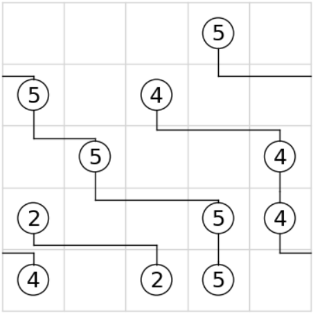
$\begin{subarray}{c}\lambda\;=\;(5,4,2)\\ \\ \operatorname{maj}(M)=4\end{subarray}$

$\begin{subarray}{c}\mu\,=\,(4,3,2,2)\\ \\ \operatorname{maj}(\rho_{N}(M))=0\end{subarray}$

$4$ $3$ $4$ $2$ $2$ $3$ $5$ $1$ $1$ $1$ $2$

$\begin{subarray}{c}\operatorname{charge}(\rho_{Q}(M))=4\\ \end{subarray}$

$\longrightarrow\;\;$     ,

We illustrate the step-by-step collapsing of the rows from bottom to top, as described after Definition 4.7: the black balls correspond to the nonwrapping partial multiline queues $N_{r}$ and the red/shaded balls are the balls of $B$ that have not yet been collapsed; the tableaux below each step correspond to the partial tableau $Q_{r}$.

The collapsing procedure acts trivially on $M\in\operatorname{MLQ}_{0}(\lambda,n)\subseteq\operatorname{\mathcal{M}_{(2)}}(\lambda_{1},n)$. Thus we have the simple, but useful lemma below.

Lemma 4.12.

Let $M\in\operatorname{MLQ}_{0}(\lambda)$. Then the tableau $\rho_{Q}(M)$ is the semistandard tableau with shape and content equal to $\lambda^{\prime}$, and it has charge 0.

By sequentially applying braid relations, we can equivalently write $\rho_{N}$ as a different sequence of operators, as follows.

Lemma 4.13.

Let $L$ and $n$ be positive integers and let $B=(B_{1},\ldots,B_{L})\in\operatorname{\mathcal{M}_{(2)}}(L,n)$. Then

$$\rho_{N}(B)=e_{[L-1,L-1]}^{\star}e_{[L-2,L-1]}^{\star}\cdots e_{[2,L-1]}^{\star}e_{[1,L-1]}^{\star}(B).$$

Proof.

Recall from the proof of 4.8 that $\rho_{N}^{(k)}=e_{[1,k-1]}^{\star}\cdots e_{[1,1]}^{\star}$ is the collapsing operator applied to the bottom $k$ rows. We will show by induction on $k$ that

$$\rho_{N}^{(k)}=e_{[k-1,k-1]}^{\star}e_{[k-2,k-1]}^{\star}\cdots e_{[1,k-1]}^{\star}.$$

The identity is trivially true for $k=1$. Supposing the result holds for $\rho_{N}^{(r)}$ with $r\geq 2$, we will show it also holds for $\rho_{N}^{(r+1)}$. Using a sequence of commutation and braid relations from Theorem 4.6, we have that for $2\leq k\leq r$,

$$e_{[1,r]}^{\star}e_{[k-1,r-1]}^{\star}=e_{[k,r]}^{\star}e_{[1,r]}^{\star}$$

We apply this relation sequentially for $k=r,r-1,\ldots,2$ to obtain

$$\rho_{N}^{(r+1)}=e_{[1,r]}^{\star}\rho_{N}^{(r)} =e_{[1,r]}^{\star}e_{[r-1,r-1]}^{\star}e_{[r-2,r-1]}^{\star}\cdots e_{[1,r-1]}^{\star}=e_{[r,r]}^{\star}e_{[1,r]}^{\star}e_{[r-2,r-1]}^{\star}\cdots e_{[1,r-1]}^{\star}$$

$$=e_{[r,r]}^{\star}e_{[r-1,r]}^{\star}e_{[1,r]}^{\star}\cdots e_{[1,r-1]}^{\star}=\ldots=e_{[r,r]}^{\star}e_{[r-1,r]}^{\star}\cdots e_{[1,r]}^{\star}.$$

Since $\rho_{N}(B)=\rho_{N}^{(L)}(B)$, we have the desired identity. ∎

Remark 4.14.

In Definition 4.7 we scan the rows of the multiline queue from bottom to top in each step of the collapsing. This can be seen from the order of the operators. In contrast, in Lemma 4.13, we start from the top and sequentially create the bottom rows of the nonwrapping multiline queue. Thus, we will refer to this version of collapsing as top-to-bottom collapsing, while to the first definition we will refer as bottom-to-top collapsing or simply collapsing.

Now we describe an alternative way to obtain the recording tableau $\rho_{Q}(B)$, by keeping track of where balls from each row of $B$ end up in $\rho_{N}(B)$, which lets us store both the insertion and recording data in the same object; we call this labelled collapsing.

Definition 4.15 (Labelled collapsing).

Let $B=(B_{1},\ldots,B_{L})\in\operatorname{\mathcal{M}_{(2)}}(L,n)$. Assign the label $r$ to each particle in $B_{r}$. Next, perform the collapsing procedure (either top-to-bottom or bottom-to-top) on the labelled configuration, and reconfigure the labels according to the following local rule: if a particle $b$ with label $\ell$ bumps a particle $b^{\prime}$ with label $k$ with $k<\ell$, swap the labels so that label $k$ stays in the current row and continue with the collapsing. After all particles are collapsed0, the final configuration of balls is $\rho_{N}(B)$ and we construct a tableau $Q^{\prime}(B)$ by reordering the row labels of the final configuration.

Remark 4.16.

The previous local rule can be restated in a more global fashion as follows to account for the collapsing of a full row on top of another, i.e. the application of $e_{i}^{\star}$ instead of a single $e_{i}$:

For a given row $i$, say $B_{i}=\{b_{1}<b_{2}<\ldots<b_{k}\}$. For a ball $b\in B_{i}$, let $S_{b}$ be the set of balls that are in row $i+1$, weakly to the left of $b$. Then in the collapsing of row $i+1$, the label of the ball that is paired to $b_{1}$ is $c_{1}\coloneqq\min(S_{b_{1}})$ and, inductively, for $2\leq j\leq k$ the label of the ball that is paired to $b_{j}$ is $c_{j}\coloneqq\min(S_{b_{j}}\setminus\{c_{1},c_{2},\ldots,c_{j-1}\}).$ To do the dropping of the remaining labels, we move the label $c_{j}$ to the ball that paired to $b_{j}$ and shift the labels of the remaining balls to the left maintaining the previous order. Then the balls that are unmatched collapse to row $i$.

See Example 4.18 for an explicit example of the previous definition. We now show that this version of collapsing coincides with the one described in Definition 4.7. Since we are using collapsing that is either bottom-to-top or top-to-bottom, Lemma 4.13 already proves that the final ball arrangement in both cases is the same. Therefore we just have to check the construction of the recording tableau.

Proposition 4.17.

For any ball arrangement $B\in\operatorname{\mathcal{M}_{(2)}}(L,n)$, the tableau $Q^{\prime}(B)$ from Definition 4.15 obtained by collapsing coincides with $\rho_{Q}(B).$

Proof.

We proceed by induction on $L$, and we analyze the cases of bottom-to-top and top-to-bottom collapsing separately. In both cases, the base case $L=2$ is trivial. Assume that labelled collapsing in produces the correct recording tableau for a ball arrangement of $L-1$ rows where $L\geq 3$. Suppose $B=(B_{1},B_{2},\ldots,B_{L})$ has $L$ rows. By assumption, for $B^{(L-1)}=(B_{1},B_{2},\ldots,B_{L-1})$ we have that $Q^{\prime}(B^{(L-1)})=\rho_{Q}(B^{(L-1)})$.

First consider the case of bottom-to-top collapsing. In the last part of the labelled collapsing of $B_{2}=(\rho_{N}(B^{(L-1)}),B_{L})$, namely when $e_{[1,L-1]}^{\star}$ acts on the ball arrangement, the possible dropping of labels occur only when a particle with label "$L$" bumps another particle. Indeed, since all the labels appearing in $\rho_{N}(B^{(L-1)})$ are less than $L$, the dropped labels are always "$L$" unless they are the only label pairing to a given ball in which case they stay in the given row. This shows that the rule described in Definition 4.15 is a reformulation of the recording tableau from Definition 4.7.

Now we focus on the case of top-to-bottom collapsing. Consider the partial collapsing $e_{[1,L-1]}^{\star}(B)$. Note that the choice of the labels that stay in each row during the labelled collapsing is the same as in $e_{[1,L-1]}^{\star}(B^{(L-1)})$ since the labels from $B_{L}$ are all "$L$". Thus, any ball in row $1$ that is in $e_{[1,L-1]}^{\star}(B)$ but not in $e_{[1,L-1]}^{\star}(B^{(L-1)})$ has label "$L$". The same argument shows that any ball that is in row $j$ of $e_{[j,L-1]}^{\star}\cdots e_{[1,L-1]}^{\star}(B)$ but not in $e_{[j,L-2]}^{\star}\cdots e_{[1,L-2]}^{\star}(B^{(L-1)})$ has label "$L$". Thus, the tableau $Q^{\prime}(B)$ is also recording the new particles that end up in each row of the previously collapsed ball arrangement, which means that it coincides with the recording tableau from Definition 4.7. ∎

Example 4.18.

We show the step-by-step labelled collapsing of the multiline queue from Example 4.11. First, we consider the case of bottom-to-top collapsing:

Now, for top-to-bottom collapsing we have the following:

Theorem 4.19.

The collapsing procedure from Definition 4.7 gives a bijection such that $x^{B}=x^{\rho_{N}(B)}$ for $B\in\operatorname{\mathcal{M}_{(2)}}(L,n)$.

Proof.

Let $B\in\operatorname{\mathcal{M}_{(2)}}(L,n)$ and let $(N,Q)=\rho(B)$. The equality $x^{B}=x^{N}$ is due to the fact that the collapsing procedure leaves the column content (and hence the $x$-weight) invariant. We will show $\rho$ is a bijection by constructing an inverse using the invertibility of the dropping operators in (19).

For $1\leq r<L-1$ with $L=\lambda_{1}$, let $B^{(r-1)}=e^{\star}_{[1,r-2]}\circ\cdots\circ e^{\star}_{[1,1]}(B)$ be a partially collapsed multiline queue. Then $e^{\star}_{[1,r-1]}(B^{(r)})$ generates the collapsing of row $r$. To construct the inverse, we shall keep track of the number of times each operator $e_{i}$ is applied within $e^{\star}_{[1,r-1]}(B^{(r-1)})$. For $1\leq j\leq r-1$, let $\phi(r,j)$ be minimal such that $e^{\star}_{[j,r-1]}(B^{(r-1)})=e^{\phi(r,j)}_{j}(e^{\star}_{[j+1,r-1]}(B^{(r-1)}))$. Then

$$B^{(r)}=e^{\star}_{[1,r-1]}(B^{(r-1)})=e^{\phi(r,1)}_{1}\circ\cdots\circ e^{\phi(r,r-1)}_{r-1}(B^{(r-1)}).$$ (20)

In particular, the sequence $(\phi(r,1),\ldots,\phi(r,r-1))$ dictates the multiset of rows containing the entries “$r$” in the recording tableau as follows: if $(m^{(r)}_{r},\ldots,m^{(r)}_{1})$ is the multiplicity vector with $m^{(r)}_{j}$ equal to the number of entries “$r$” in row $j$ of $Q$, then $m^{(r)}_{j}=\phi(r,j)-\phi(r,j-1)$, where $\phi(r,r)=\lambda_{r}^{\prime}$ and $\phi(r,0)=0$.

By minimality of the $\phi(r,j)$’s, each $e_{j}^{\phi(r,j)}$ is invertible with inverse $f_{j}^{\phi(r,j)}$, and thus

$$f^{\phi(r,r-1)}_{r-1}\circ\cdots\circ f^{\phi(r,1)}_{1}(M_{r})=M_{r-1}.$$

Therefore, to construct $\rho^{-1}(N,Q)$ from $(N,Q)\in\operatorname{MLQ}_{0}(\mu,n)\times\operatorname{SSYT}(\mu^{\prime},\lambda^{\prime})$ for some partition $\mu$, we define the tuples $(\phi(r,j)\colon 1\leq j<r)$ from the multiplicity vectors $(m_{j}^{(r)}\colon 1\leq j\leq r)$ in $Q$ for $2\leq r\leq L$ , and set

$$\rho^{-1}(N,Q)=\bigcirc_{r=2}^{L}\left(f^{\phi(r,r-1)}_{r-1}\circ\cdots\circ f^{\phi(r,2)}_{2}\circ f^{\phi(r,1)}_{1}\right)(N).$$ (21)

where the notation $\bigcirc_{i=a}^{b}Y_{i}(N)$ represents the composition $Y_{b}\circ\cdots\circ Y_{a+1}\circ Y_{a}(N)$.

By (20), the composition of (21) with (19) is the identity, so $\rho^{-1}$ is a left inverse of $\rho$. A similar argument shows this is also a right inverse of $\rho$.∎

In fact, the bijection $\rho$ can be directly considered an analogue of RSK on multiline queues, since the lifting operators required to recover the corresponding multiline queue are read from the tableau $Q$, in the same way as one would construct the inverse RSK map. In Section 5, we will interpret collapsing as a map from multiline queues to pairs of nonwrapping multiline queues, to strengthen the comparison with RSK.

We restrict the collapsing procedure to the set of multiline queues $\operatorname{MLQ}(\lambda,n)$, identified as the set of binary matrices on $n$ columns with row content given by $\lambda^{\prime}$. Endowing this set with the weight $\operatorname{wt}(M)=q^{\operatorname{maj}(M)}x^{M}$ gives the following map.

Theorem 4.20.

Let $\lambda$ be a partition and $n\geq\ell(\lambda)$ a positive integer. Then collapsing restricted to $\operatorname{MLQ}(\mu,n)$ is a weight-preserving bijection with $x^{|M|}=x^{\rho_{N}(M)}$ and $\operatorname{maj}(M)=\operatorname{charge}(\rho_{Q}(M))$:

$$\rho\;\colon\;\operatorname{MLQ}(\mu,n)\;\longrightarrow\;\bigcup_{\lambda}\operatorname{MLQ}_{0}(\lambda,n)\times\operatorname{SSYT}(\lambda^{\prime},\mu^{\prime})\\$$ (22)

From this theorem, we recover the expansion of $q$-Whittaker polynomials in the Schur basis, and can derive a multiline queue formula for $K_{\lambda\mu}(q)$.

Definition 4.21.

For partitions $\nu$ and $\eta$, let $\operatorname{MLQ}(\nu,\eta)=\{M\in\operatorname{MLQ}(\nu)\colon x^{M}=x^{\eta}\}$ be the set of multiline queues of shape $\nu$ with column content $\eta$. Also, let $M(\nu)$ be the (unique) left-justified multiline queue of shape $\nu$. That is, $M(\nu)=(M_{1},\ldots,M_{\nu_{1}})$ with $M_{j}=\{1,2,\ldots,\nu^{\prime}_{j}\}$ for $1\leq j\leq\nu_{1}$.

Corollary 4.22.

Let $\lambda$ and $\mu$ be partitions. Then

$$K_{\lambda\mu}(q,0)=\sum_{\begin{subarray}{c}M\in\operatorname{MLQ}(\mu,\lambda^{\prime})\\ \operatorname{\rho_{N}}(M)=M(\lambda^{\prime})\end{subarray}}q^{\operatorname{maj}(M)}$$

Proof.

For some partitions $\lambda,\mu$, consider the set $\operatorname{MLQ}_{0}(\lambda)\times\operatorname{SSYT}(\lambda^{\prime},\mu^{\prime})$, which has generating function $s_{\lambda}(X)K_{\lambda\mu}(q,0)$. For $A\in\operatorname{MLQ}_{0}(\lambda,n)$, the preimage under $\rho$ of the set $\{A\}\times\operatorname{SSYT}(\lambda^{\prime},\mu^{\prime})$ is $\{M\in\operatorname{MLQ}(\mu):\rho_{N}(M)=A\}$, which has generating function $x^{A}K_{\lambda\mu}(q,0)$. Therefore, to extract the coefficient $[s_{\lambda}]P_{\mu}(X;q,t)$, it is sufficient to sum over the preimage of the set $\{A\}\times\operatorname{SSYT}(\lambda^{\prime},\mu^{\prime})$ for any choice of $A\in\operatorname{MLQ}_{0}(\lambda,n)$, the simplest of which is $A=M(\lambda)$.

∎

We record an useful characterization of the special multiline queues $M(\lambda)$. Recall that a word is a lattice word if each initial segment contains at least as many letters "$i$" as letters "$i+1$" for every $i\geq 1$.

Lemma 4.23.

Let $M\in\operatorname{MLQ}(\mu,\lambda^{\prime})$. Then $\rho_{N}(M)=M(\lambda^{\prime})$ if and only if $\operatorname{rw}(M)$ is a lattice word.

Proof.

Suppose that $\operatorname{rw}(M)$ is a lattice word. We show that $\rho_{N}(M)=M(\lambda^{\prime})$ by induction on the length of the row word. If $\operatorname{rw}(M)$ has length one, then $\operatorname{rw}(M)=1$ and the collapsing is trivially left justified. Now suppose $\operatorname{rw}(M)=r_{1}\,r_{2}\,\ldots\,r_{n-1}\,r_{n}=:w\,r_{n}.$ Note that $w$ is also a lattice word, and by induction the collapsing of the multiline queue restricted to $M$ is $M(\mu)$ for some partition $\mu$. Say $\mu$ has multiplicity vector $(m_{1},m_{2},\ldots,m_{k})$. Then by the lattice condition on $\operatorname{rw}(M)$, $r_{n}=\sum_{i=1}^{j}m_{i}+1$ for some $1\leq j\leq k$. Therefore, the collapsing of the ball corresponding to $r_{n}$ on $M(\mu)$ yields a left-justified multiline queue.

Suppose that $\operatorname{rw}(M)$ is not a lattice word. Then take the first initial segment $\widetilde{r}$ of $\operatorname{rw}(M)$ in which the lattice condition does not hold. Say that the number $c$ is such that $\widetilde{r}$ has more "$c$"s than "$c-1$"s. Thus, $\widetilde{r}=w\,c$ where $w$ is a lattice word (that may be empty). Then the collapsing of the partial multiline queue $\widetilde{M}$ obtained from restricting to the balls recorded to $\widetilde{r}$ yields a left-justified multiline queue when the balls corresponding to $w$ are collapsed, and when the last ball at column $c$ collapses, since there are less balls in column $c-1$, it will not be left justified. Hence, $\rho_{N}(M)\neq M(\lambda^{\prime})$.

∎

We end this section by examining some properties of collapsing on generalized multiline queues (binary matrices with arbitrary row content).

Proposition 4.24.

For a composition $\alpha$ and $B\in\operatorname{GMLQ}(\alpha)$, $\rho(B)=\rho(\sigma_{i}(B))$ for any $i\geq 1$.

Proof.

Write $B^{\prime}=\sigma_{i}(B)$. Without loss of generality, assume $\alpha_{i+1}>\alpha_{i}$ (if $\alpha_{i}=\alpha_{i+1}$, the claim is trivial since $B=B^{\prime}$).

Let $A\subseteq B_{i+1}$ and $C\subseteq B_{i}$ be the sets of particles matched above and below, respectively, in $\operatorname{\pi}^{c}(B_{i+1},B_{i})$. Note that these are also the sets matched above and below in $\operatorname{\pi}^{c}(B^{\prime}_{i+1},B^{\prime}_{i})$ by the definition of $\sigma_{i}$. Let $D$ be the set of particles that is moved between rows $i$ and $i+1$ by the involution $\sigma_{i}$ (i.e. the set of unmatched particles above in $\operatorname{\pi}^{c}(B_{i+1},B_{i})$ and below in $\operatorname{\pi}^{c}(B^{\prime}_{i+1},B^{\prime}_{i})$, respectively). Then $B_{i}=C$, $B_{i+1}=A\cup D$, $B^{\prime}_{i}=C\cup D$, and $B^{\prime}_{i+1}=A$.

Balls matched above (resp. below) in $\operatorname{\pi}(X,Y)$ are necessarily also matched above (resp. below) in $\operatorname{\pi}^{c}(X,Y)$. Thus a ball is matched above in $\operatorname{\pi}(A,C\cup D)$ only if it is matched above in $\operatorname{\pi}^{c}(A,C\cup D)$, which is true only if it is matched above in $\operatorname{\pi}^{c}(A\cup D,C)$. Since no ball in $D$ is matched, every ball matched above in $\operatorname{\pi}(A\cup D,C)$ must also be matched above in $\operatorname{\pi}(A,C\cup D)$. Thus the set of balls matched above in $\operatorname{\pi}(B^{\prime}_{i+1},B^{\prime}_{i})$ is equal to the set of balls matched above in $\operatorname{\pi}(B_{i+1},B_{i})$, which implies that $e_{i}^{\star}(\sigma_{i}(B))=e_{i}^{\star}(B)$.

Now we write $\rho=e_{[1,L]}^{\star}\cdots e_{[1,i+1]}^{\star}\rho^{(i+1)}_{N}$. Since the first operator applied in $\rho^{(i+1)}_{N}$ is $e_{i}^{\star}$, from the above we have that $\rho^{(i+1)}_{N}\circ\sigma_{i}(B)=\rho^{(i+1)}_{N}(B)$, from which we get $\rho(\sigma_{i}(B))=\rho(B)$. ∎

Remark 4.25.

There are strong correspondences of collapsing to Robinson–Schensted insertion of the (row and column) (bi)words of the multiline queue. Let $B\in\operatorname{\mathcal{M}_{(2)}}(L,n)$ be a binary matrix. Then

$$\operatorname{dualRSK}\left(B_{r}(B)\right)=(\operatorname{tab}(B),\rho_{Q}(B)),$$

where the map $\operatorname{tab}:\operatorname{MLQ}\rightarrow\operatorname{SSYT}$ is defined in Appendix A. Based on Remark 3.3, $\operatorname{cw}(B)$ is the bottom row of $\overline{B_{c}}(B)$. With $\operatorname{dualRSK}(B_{r}(B))=(P,Q)$, we have the identity $\operatorname{BurgeRSK}(\overline{B_{c}}(B))=(Q,P)$ due to [15, Symmetry Theorem (b)]. Then it follows that

$$\rho_{Q}(B)=\operatorname{I_{row}}(\operatorname{cw}(B)).$$

Furthermore, recall that for $i\geq 1$, the Lascoux–Schützenberger operator $S_{i}$ acts on semistandard tableaux $T\in\operatorname{SSYT}$ by applying the Lascoux–Schützenberger involution on the word $\operatorname{crw}(T)$ and changing the corresponding entries of $T$ to obtain $S_{i}\cdot T$. Then we have

$$\rho_{Q}(\sigma_{i}(B))=S_{i}\cdot\rho_{Q}(B).$$

4.1.1 Nonwrapping generalized multiline queues

It is natural to define generalized nonwrapping multiline queues, the twisted analogue of $\operatorname{MLQ}_{0}(\lambda)$.

Definition 4.26.

For a composition $\alpha$, define the set of nonwrapping generalized multiline queues as

$$\operatorname{GMLQ}_{0}(\alpha)=\{B\in\operatorname{GMLQ}(\alpha):\operatorname{maj}_{G}(B)=0\}.$$

We claim that $B\in\operatorname{GMLQ}_{0}(\alpha,n)$ if and only if it has no wrapping pairings under the left-to-right pairing order convention of Definition 3.25, hence justifying the choice of the name for these objects. We give a sketch of the argument: first, for any generalized multiline queue, within each pair of rows, the number of particle pairings wrapping to the right must equal the number of anti-particle pairings wrapping to the left. Second, if $\operatorname{maj}_{G}(B)=0$, the contribution to $\operatorname{maj}_{G}$ from each pair of rows is 0. Since the label of any anti-particle is less than or equal to the label of any particle, in order to get a sum of zero from the particle and anti-particle contributions within each pair of rows, the only possibility is that all wrapping pairings come from particles or anti-particles of the same label (i.e. the smallest label pairing in the particle phase), which necessarily cancel each other out. However, this means the left to right pairing order during the particle phase will necessarily prevent any wrapping particle pairings. In particular, this last fact implies that to check that a generalized multiline queue has $\operatorname{maj}_{G}$ equal to 0, it is sufficient to only check for particle pairings wrapping to the right.

From 4.24, we obtain the following commuting diagram.

The composition $\sigma\circ\rho_{N}^{\downarrow}\circ\sigma^{-1}$ defines a map $\rho_{\sigma}^{\downarrow}\colon\operatorname{GMLQ}(\alpha)\longrightarrow\bigcup_{\beta}\operatorname{GMLQ}_{0}(\beta)$ where the union runs over all compositions $\beta$ such that $\sigma^{-1}\cdot\beta\leq\sigma^{-1}\cdot\alpha$ with respect to dominance order on partitions. For a concrete example, see Example 4.28.

Question 4.27.

Give a combinatorial description of the map $\rho_{\sigma}^{\downarrow}$ on generalized multiline queues that is analogous to Definition 4.7.

Example 4.28.

For $\lambda=(4,4,3,2,1)$ and $\sigma=4\,2\,1\,5\,3=s_{3}\,s_{2}\,s_{1}\,s_{2}\,s_{4}$, the twisting of the partition $\lambda$ is the composition $\alpha=\sigma\cdot\lambda=(3,4,1,4,2)$. For $M\in\operatorname{GMLQ}(\lambda,6)$, we show the generalized multiline queue $B=\sigma(M)\in\operatorname{GMLQ}(\alpha,6)$, and the corresponding collapsed generalized multiline queues $\rho^{\downarrow}_{\sigma}(B)$ and $\rho^{\downarrow}(M)$. Note that $\rho_{N}^{\downarrow}(B)=\rho_{N}^{\downarrow}(M)$ in accordance with 4.24.

4.2 Formulas for $P_{\lambda}(X;q,0)$ via generalized multiline queues

In this section, we define the statistic $\operatorname{maj}_{G}$ as the analogue of $\operatorname{maj}$ for generalized multiline queues in which we think of particles as pairing to the right and anti-particles as pairing to the left, with every pairing wrapping to the right contributing a positive term to the major index, and every pairing wrapping to the left contributing a negative term. We then generalize results of [1] to obtain a family of formulas for the $q$-Whittaker polynomials as a sum over generalized multiline queues with the $\operatorname{maj}_{G}$ statistic.

Definition 4.29.

Let $M\in\operatorname{GMLQ}(\alpha,n)$ with an associated labelling $L(M)$. For $1\leq r,\ell\leq L$, let $m_{r,\ell}$ (resp. $a_{r,\ell}$) be the number of particles (resp. anti-particles) of type $\ell$ that wrap when pairing to the right (resp. left) from row $r$ to row $r-1$, as shown in Example 4.31. Define

$$\operatorname{maj}_{G}(M)=\sum_{1\leq r,\ell\leq L}m_{r,\ell}(\ell-r+1)-a_{r,\ell}(\ell-r+1).$$ (23)

Lemma 4.30.

When $M\in\operatorname{MLQ}(\lambda,n)$, $\operatorname{maj}_{G}(M)=\operatorname{maj}(M)$.

Proof.

The particle phase of Definition 3.25 is identical to the FM algorithm. Thus when $M$ is a straight multiline queue, the labelling of the particles is identical to that in Definition 3.11, and so $L_{G}(M)^{+}=L(M)$. Furthermore, for $1\leq r\leq\lambda_{1}$, one may check that all anti-particles in row $r$ are labelled $r-1$ in $L_{G}(M)$. Thus the contribution to $\operatorname{maj}$ from anti-particles wrapping during either phase of the generalized pairing procedure is $(r-1)-r+1=0$. Therefore, only wrapping particles contribute to $\operatorname{maj}_{G}(M)$, and the contribution is identical to that for $\operatorname{maj}(M)$. ∎

Example 4.31.

For $\alpha=(2,2,3)$, the labelled particles (circles) and anti-particles (squares) are shown for $M=(\{2,3\},\{1,4\},\{2,3,4\})\in\operatorname{GMLQ}(\alpha,4)$, $\sigma_{2}(M)=(\{2,3\},\{1,2,4\},\{3,4\})\in\operatorname{GMLQ}(s_{2}\cdot\alpha,4)$ and $\sigma_{1}(\sigma_{2}(M))=(\{2,3,4\},\{1,2\},\{3,4\})\in\operatorname{GMLQ}(s_{1}s_{2}\cdot\alpha,4)$. The positive (blue) and negative (red) contributions to $\operatorname{maj}_{G}$ are shown, totalling $\operatorname{maj}_{G}=2$ in each case.

The main result of [1] states that the involution $\sigma_{i}$ preserves the labelling of the bottom row of a generalized multiline queue, thus preserving the distribution of states of the multispecies ASEP onto which the generalized multiline queues project, and thereby giving a twisted analogue of (12). We claim that the $\operatorname{maj}_{G}$ statistic is also preserved under $\sigma_{i}$. We will show that our definition of $\operatorname{maj}_{G}$ can be reformulated in terms of an energy function on tensors of KR crystals that was introduced in [26].

Definition 4.32.

Let $w$ be a word in $\{0,1,\ldots,L\}$ in $n$ letters and let $D\subseteq[n]$ represent a row of a generalized multiline queue. Define

$$\operatorname{maj}_{G}(w;D)=\sum_{a}\left(\ell(a)-i\right)-\sum_{b}\left(\ell(b)-i\right)$$ (24)

where the first sum is over all pairings $a$ wrapping (to the right) during the particle phase and the second is over all pairings $b$ wrapping during the anti-particle phase at that row.

In a generalized multiline queue $M=(B_{1},\ldots,B_{L})$, if we let $w^{(i)}$ be the labelling word of row $i$ in $L_{G}(M)$, then $\operatorname{maj}_{G}(w^{(i+1)};B_{i})$ is the contribution to $\operatorname{maj}_{G}(M)$ of the pairings from row $i+1$ to row $i$, and thus we may write

$$\operatorname{maj}_{G}(M)=\sum_{i=1}^{L-1}\operatorname{maj}_{G}(w^{(i+1)};B_{i}).$$

Definition 4.33.

Let $w$ be a word in $\{0,1,\ldots,L\}$. The nested indicator decomposition of $w$ is the set of words $\{w_{1},w_{2},\ldots,w_{L}\}$ given by $w_{j}=w_{j1}\,w_{j2}\,\ldots\,w_{jn}\in\{0,1\}^{n}$ where $w_{jk}=1$ if and only if the $k$-th entry of $w$ is greater than or equal to $j$, so that $w=w_{1}+\cdots+w_{L}$ if addition is performed componentwise. For an indicator word $u\in\{0,1\}^{n}$, define $\iota(u)$ to be the subset of $[n]$ associated to $u$: $\iota(u)=\{i\in[n]:u_{i}=1\}$. In particular, $w_{1},\ldots,w_{L}$ are nested indicator words if and only if $\iota(w_{L})\subseteq\cdots\subseteq\iota(w_{2})\subseteq\iota(w_{1})$.

Example 4.34.

For $w=2\,5\,2\,3\,4\,2$ the nested indicator decomposition is:

$$w_{1}=w_{2}=1\,1\,1\,1\,1\,1,\ w_{3}=0\,1\,0\,1\,1\,0,\ w_{4}=0\,1\,0\,0\,1\,0,\ \mbox{and}\ w_{5}=0\,1\,0\,0\,0\,0.$$

The corresponding subsets are

$$\iota(w_{1})=\iota(w_{2})=\{1,2,3,4,5,6\},\ \iota(w_{3})=\{2,4,5\},\ \iota(w_{4})=\{2,5\},\ \mbox{and}\ \iota(w_{5})=\{2\}.$$

Definition 4.35.

Given a queue $D\subseteq[n]$ and a word $w\in\{0,1,\ldots,L\}^{n}$ with nested indicator decomposition $w=w_{1}+\cdots+w_{L}$, the energy function $H(w_{j};D)$ is defined as the number of wrapping pairings in $\operatorname{\pi}^{c}(D,\iota(w_{j}))$. Then, define $H(w;D)\coloneqq\sum_{j=1}^{L}H(w_{j};D)$. Finally, for a multiline queue $M=(B_{1},\ldots,B_{L})$ with $L_{G}(M)=(w^{(1)},\ldots,w^{(L)})$, define $H(M)\coloneqq\sum_{i=1}^{L-1}H(w^{(i+1)};B_{i})$

Remark 4.36.

Definition 4.35 is a translation of the energy function as defined in [26], though the authors only consider objects corresponding to straight multiline queues in their paper. However, it is immediate that the energy function is invariant of the action of the combinatorial R matrix (directly corresponding to our $\sigma_{i}$), which defines a crystal isomorphism; thus the energy function can be defined in our setting as well. Moreover, we have that $H(M)=H(\sigma_{i}(M))$ for any (generalized) multiline queue $M$.

Example 4.37.

Consider the generalized multiline queue $M=(\{2,3\},\{1,4\},\{2,3,4\})$ from Example 4.31. Then

$$L(G)=(w^{(1)}=0\,3\,3\,1\,,\,w^{(2)}=3\,2\,1\,3\,,\,w^{(3)}=2\,3\,3\,3)$$

and the computation of the energy function $H(M)=2$ can be decomposed as follows:

$w^{(3)}=2\,3\,3\,3$	$B_{2}=1\,0\,0\,1$	$w^{(2)}=3\,2\,1\,3$	$B_{1}=0\,1\,1\,0$
$w^{(3)}_{1}=1\,1\,1\,1$	$H(w^{(3)}_{1},B_{2})=0$	$w^{(2)}_{1}=1\,1\,1\,1$	$H(w^{(2)}_{1},B_{1})=0$
$w^{(3)}_{2}=1\,1\,1\,1$	$H(w^{(3)}_{2},B_{2})=0$	$w^{(2)}_{2}=1\,1\,0\,1$	$H(w^{(2)}_{2},B_{1})=0$
$w^{(3)}_{3}=0\,1\,1\,1$	$H(w^{(3)}_{3},B_{2})=1$	$w^{(2)}_{3}=1\,0\,0\,1$	$H(w^{(2)}_{3},B_{1})=1$

Definition 4.38.

For a word $w$, let $\operatorname{rev}(w)$ be the reversed word with letters $\operatorname{rev}(w)_{i}=w_{n-i+1}$. For a subset $S\subseteq[n]$ let $\operatorname{rev}(S)=\{n-i+1\,\colon\,i\in S\}$ be the reversed version of $S$ in $[n]$.

Proposition 4.39.

In the setup of Definitions 4.32 and 4.33, let $w=w_{1}+\cdots+w_{L}$ be the decomposition of a word $w$ into nested indicator vectors, and let $D\subseteq[n]$ be a queue. Then

$$\operatorname{maj}_{G}(w\,;D)=\sum_{j=1}^{L}H(w_{j}\,;D).$$ (25)

In particular, this implies that for a generalized multiline queue $M$, we have $\operatorname{maj}_{G}(M)=H(M)$.

Proof.

For an indicator word $v\in\{0,1\}^{n}$ and a set of balls $D\subseteq[n]$, denote by $\overline{D}$ the complement of $D$ in $[n]$ and by $\overline{v}$ the complement of the word $v$ with letters $\overline{v}_{i}=1-v_{i}$. Define an anti-particle energy function, $H^{\leftarrow}(v\,;D)$ as the number of wrapping pairings in $\operatorname{\pi}^{c}(\operatorname{rev}(D),\operatorname{rev}(v))$. We interpret this energy function as counting the number of wrapping pairings to the left in the two-row arrangement $(D,\iota(v))$. We claim that $H^{\leftarrow}(\overline{v}\,;\overline{D})=H(v\,;D)$. This can be seen from the identity $H^{\leftarrow}(\overline{v}\,;\overline{D})=H(\iota^{-1}(\overline{D})\,;\iota(\overline{w}))$ and the fact that a wrapping particle in $\operatorname{\pi}^{c}(D,\iota(v))$ unbalances the number of anti-particles to its right creating a wrapping in $\operatorname{\pi}^{c}(\iota(\overline{w}),\overline{D}).$

Let $w=w_{1}+w_{2}+\cdots+w_{L}$ be the word labelling row $i$ of $L_{G}(M)$, let $D$ be the queue at row $i-1$, and consider $\operatorname{maj}_{G}(w;D)$ (note that we have decremented the index for nicer computations). We will write $h^{\rightarrow}_{j}\coloneqq H(w_{j};D)$ and $h^{\leftarrow}_{j}\coloneqq H^{\leftarrow}(\overline{w_{j}};\overline{D})$. Define $\ell=\min_{j}\{|\iota(w_{j+1})|<|D|\leq|\iota(w_{j})|\}$ to be the smallest label of a ball that pairs during the particle phase in row $i$ of $L_{G}(M)$. Let us decorate the letters $\ell$ in $w$: label the $\ell$’s that pair during the particle phase by $\ell^{+}$ and those that pair during the anti-particle phase by $\ell^{-}$, and let those sites be indexed by the indicator vectors $u_{\ell^{+}},u_{\ell^{-}}$ so that $w_{\ell}=w_{\ell+1}+u_{\ell^{+}}+u_{\ell^{-}}$. Now, by comparing definitions, we observe that

$$m_{i,j} =h^{\rightarrow}_{j}-h^{\rightarrow}_{j+1}, \mbox{if}\ \ell<j\leq L\qquad\qquad\mbox{and}\ m_{i,\ell} =h^{\rightarrow}_{\ell^{+}}-h^{\rightarrow}_{\ell+1}$$

$$a_{i,j} =h^{\leftarrow}_{j}-h^{\leftarrow}_{j+1}, \mbox{if}\ i-1\leq j<\ell\qquad\qquad\mbox{and}\ a_{i,\ell} =h^{\leftarrow}_{\ell^{+}}-h^{\leftarrow}_{\ell}.$$

with $h^{\rightarrow}_{L+1}\coloneqq 0$, where $m_{i,j}$ and $a_{i,j}$ are the quantities in Definition 4.29. Plugging these into (24), we obtain

$$\operatorname{maj}_{G}(w;D) =\sum_{j=\ell}^{L}m_{i,j}(j-i+1)-\sum_{j=i-1}^{\ell}a_{i,j}(j-i+1)$$

$$\begin{aligned} =m_{i,\ell}(\ell-i+1)&+\sum_{j=\ell+1}^{L}(h^{\rightarrow}_{j}-h^{\rightarrow}_{j+1})(j-i+1)\\ &-a_{i,\ell}(\ell-i+1)-\sum_{j=i-1}^{\ell-1}(h^{\leftarrow}_{j}-h^{\leftarrow}_{j+1})(j-i+1)\end{aligned}$$

$$\begin{aligned} =(-h^{\rightarrow}_{\ell+1}+h^{\leftarrow}_{\ell})(\ell-i+1)&+h^{\rightarrow}_{\ell+1}(\ell+1-i+1)-h^{\rightarrow}_{L+1}(L-i+1)\\ &+\sum_{j=\ell+2}^{L}(h^{\rightarrow}_{j}(j-i+1)-h^{\rightarrow}_{j}((j-1)-i+1))\\ &-\sum_{j=i}^{\ell-1}(h^{\leftarrow}_{j}((j-1)-i+1)-h^{\leftarrow}_{j}(j-i+1))\\ &+h^{\leftarrow}_{i-1}((i-1)-i+1)-h^{\leftarrow}_{\ell}((\ell-1)-i+1)\end{aligned}$$

$$=h^{\rightarrow}_{\ell+1}+h^{\leftarrow}_{\ell}+\sum_{j=\ell+2}^{L}(h^{\rightarrow}_{j})-\sum_{j=i}^{\ell-1}(-h^{\leftarrow}_{j})=\sum_{j=i}^{L}h^{\leftarrow}_{j}$$

The last equality follows from $h^{\leftarrow}_{j}=h^{\rightarrow}_{j}$. It should be noted that if $w$ is the labelling word of row $i$ of $L_{G}(M)$, then it only contains the letters $\{i-1,\ldots,L\}$, which determines the indices of the sums. Since $H(w_{j};D)=0$ for all $j<i$, we obtain the right hand side of (25).

∎

Corollary 4.40.

Let $\alpha$ be a composition with $\alpha^{+}=\lambda^{\prime}$, $L\coloneqq\ell(\alpha)$, $M\in\operatorname{GMLQ}(\alpha)$, and let $1\leq i\leq L-1$. Then $\operatorname{maj}_{G}(M)=\operatorname{maj}_{G}(\sigma_{i}(M))$.

Proof.

From 4.39, we have that $\operatorname{maj}_{G}(M)=H(M)=H(\sigma_{i}(M))=\operatorname{maj}_{G}(\sigma_{i}(M))$, where the $\sigma_{i}$-invariance of $H$ is explained in Remark 4.36. ∎

Proposition 4.41.

Let $\alpha$ be a composition and let $M\in\operatorname{GMLQ}(\alpha)$. Then $\operatorname{maj}_{G}(M)=\operatorname{charge}_{G}(\operatorname{cw}(M))$.

Proof.

From Lemma 4.30 and Theorem 4.9, this is true for a straight multiline queue. Since the left hand side is invariant under the action of $\sigma_{i}$ by Corollary 4.40, it is enough to show that is true for the right hand side, as well. By definition, $\operatorname{charge}_{G}$ is invariant under the action of $\operatorname{LS}_{i}$ on the column reading word, so we have $\operatorname{charge}_{G}(\operatorname{cw}(M))=\operatorname{charge}_{G}(\operatorname{LS}_{i}(\operatorname{cw}(M)))=\operatorname{charge}_{G}(\operatorname{cw}(\sigma_{i}(M)))$, proving our claim. ∎

By Lemmas 3.32, 4.40 and 4.9, we obtain Theorem 4.42.

Theorem 4.42.

Let $\lambda$ be a partition, $n$ an integer, and let $\alpha$ be a composition with $\alpha^{+}=\lambda^{\prime}$. Then

$$P_{\lambda}(X;q,0)=\sum_{M\in\operatorname{GMLQ}(\alpha,n)}q^{\operatorname{maj}_{G}(M)}x^{M}.$$

Remark 4.43.

There is an analogous NY rule for bosonic multiline queues, which are multiline queues with any number of particles per site; the rule naturally arises from the rank-level duality property of KR crystals of affine type (see, e.g. [19]). This can be used to obtain analogous results for $\widetilde{H}_{\lambda}(X;q,0)$ in terms of a charge statistic defined on generalized bosonic multiline queues, which we will explore in follow-up work [24].

5 Multiline queue analogues of the RSK correspondence

Recall that Theorem 4.19 is a bijection involving multiline queues and tableaux. In this section, we describe an analogue of the RSK correspondence in which all objects are multiline queues. These descriptions are equivalent to the double crystals considered in [29] due to the relation between collapsing and raising/lowering operators described in Section 5.1. However, in the context of multiline queues this becomes a very useful tool to give a simple proof of the charge formula in Theorem 4.9 and to derive the expression for $K_{\lambda\mu}(q,0)$ in terms of multiline queues.

5.1 Multiline queue RSK via commuting crystal operators

We shall describe an analogue of the Robinson–Schensted–Knuth bijection for multiline queues. We define two operators $\rho^{\downarrow}$ and $\rho^{\leftarrow}$ acting on $\operatorname{\mathcal{M}_{(2)}}$ and a $90^{\circ}$ rotation of it by treating the elements of this set as (generalized) multiline queues, and collapsing them both. This is equivalent to collapsing the multiline queue in two directions: downwards and to the left, respectively.

Remark 5.1.

There are several choices that can be made in how an element of $\operatorname{\mathcal{M}_{(2)}}$ is interpreted as a multiline queue, and each results in some variation of the results. These include:

• The pair of collapsing directions can be any orthogonal pair in the set $\{\uparrow\;,\;\downarrow\;,\;\leftarrow\;,\,\rightarrow\}$.

• Balls can be paired either weakly to the right or weakly to the left.

We will analyze the case of collapsing downwards and to the left: collapsing downwards is consistent with the previous sections, and collapsing to the left gives an elementary proof of Theorem 4.9. Moreover, the pair (down, left) yields a symmetry as shown in 5.8.

Definition 5.2.

For $B\in\operatorname{\mathcal{M}_{(2)}}$, define $\operatorname{rot}(B)$ to be the rotation of $B$ by $90^{\circ}$ counterclockwise. Define the downward and leftward collapsing of $B$, denoted $\rho^{\downarrow}(B)$ and $\rho^{\leftarrow}(B)$, respectively:

$$\rho^{\downarrow}(B)\coloneqq \rho_{N}(B),$$

$$\rho^{\leftarrow}(B)\coloneqq \operatorname{rot}^{-1}(\rho_{N}(\operatorname{rot}(B))).$$

Example 5.3.

For the matrix $B\in\operatorname{\mathcal{M}_{(2)}}(5,6)$ in the upper left, we show $\rho^{\leftarrow}(B)\in\operatorname{MLQ}_{0}(\lambda^{\prime},5)$, $\rho^{\downarrow}(B)\in\operatorname{MLQ}_{0}(\lambda,6)$, and $\rho^{\downarrow}(\rho^{\leftarrow}(B))=M(\lambda)=\in\operatorname{MLQ}_{0}(\lambda,5)$ for $\lambda=(5,3,2,2,1)$.

Theorem 5.4.

Let $L,n$ be positive integers. Define the map

$$\operatorname{mRSK}\;:\;\operatorname{\mathcal{M}_{(2)}}(L,n)\longrightarrow\bigcup_{\lambda}\operatorname{MLQ}_{0}(\lambda,n)\times\operatorname{MLQ}_{0}(\lambda^{\prime},L),$$

where the union is over partitions $\lambda$ with $\ell(\lambda)\leq n$ and $\ell(\lambda^{\prime})\leq L$, by $\operatorname{mRSK}(B)=(\rho^{\leftarrow}(B),\rho^{\downarrow}(B))$. Then $\operatorname{mRSK}$ is a bijection.

To prove Theorem 5.4 we need some preliminary results. For now, we mention that the theorem immediately gives the following identity.

Corollary 5.5 (Dual Cauchy identity).

$$\sum_{\lambda}s_{\lambda}(x)s_{\lambda^{\prime}}(y)=\prod_{i,j}(1+x_{i}y_{j}).$$

Proof.

Assign to $B\in\operatorname{\mathcal{M}_{(2)}}$ the weight function $\operatorname{wt}(B)=\prod_{i,j\geq 1}(x_{i}y_{j})^{B_{i,j}}$, so that the right hand side is the weight generating function over $\operatorname{\mathcal{M}_{(2)}}$. With the weight $\operatorname{wt}(N_{1},N_{2})=x^{N_{1}}y^{N_{2}}$ for $(N_{1},N_{2})\in\operatorname{MLQ}_{0}(\lambda)\times\operatorname{MLQ}_{0}(\lambda^{\prime})$, the generating function of the codomain of $\operatorname{mRSK}$ is

$$\sum_{\lambda}\sum_{\begin{subarray}{c}N_{1}\in\operatorname{MLQ}_{0}(\lambda)\\ N_{2}\in\operatorname{MLQ}_{0}(\lambda^{\prime})\end{subarray}}x^{N_{1}}y^{N_{2}}.$$

From (14), this generating function equals the expression on the left hand side of the Cauchy identity. The identity follows since $\operatorname{mRSK}$ is weight-preserving.∎

We now focus on proving Theorem 5.4. We show that orthogonal dropping operators commute, and then conclude that we can regard one of the collapsed multiline queues as a recording object in the usual RSK sense.

Definition 5.6.

Define the operator $e_{i}^{d}$ for $d\in\{\uparrow\;,\;\downarrow\;,\;\leftarrow\;,\,\rightarrow\}$ as the dropping operator in the direction $d$ acting on $\operatorname{\mathcal{M}_{(2)}}$ by moving all unmatched above balls from row $i$ to row $i-1$, where rows are numbered with respect to the orientation $d$. Given that we can rotate and reflect any matrix to apply the operators, we restrict to studying the downwards and leftwards directions. Explicitly, $e_{i}^{\downarrow}\coloneqq e_{i}^{\star}$ from Section 4.1 and $e_{i}^{\leftarrow}\coloneqq\operatorname{rot}^{-1}\circ\,e_{i}^{\star}\circ\operatorname{rot}$.

For any direction $d$, we write $e_{[a,b]}^{d}\coloneqq e_{b}^{d}e_{b-1}^{d}\cdots e_{a}^{d}$ for the composition of a sequence of operators, and define

$$\rho_{N}^{d}(B)\coloneqq e_{[1,L-1]}^{d}e_{[1,L-2]}^{d}\cdots e_{[1,2]}^{d}e_{[1,1]}^{d}(B).$$

The following fact that the operators $e_{i}^{\downarrow}$ and $e_{i}^{\leftarrow}$ commute can be deduced from [29, Lemma 1.3.7], but we provide a self-contained proof to align with our particular definitions.

Lemma 5.7.

Let $B\in\operatorname{\mathcal{M}_{(2)}}$. Then $e_{i}^{\downarrow}(e_{j}^{\leftarrow}(B))=e_{j}^{\leftarrow}(e_{i}^{\downarrow}(B))$ for all $i$ and $j$.

Proof.

Let $X$ be a (possibly empty) set of balls in $B_{i+1}$ that are unmatched above. Let $Y$ be the (possibly empty) set of balls in row $j+1$ of $\operatorname{rot}(B)$ (i.e. column $j+1$ of $B$) that are unmatched above. Then $e_{i}^{\downarrow}(B)$ is $B$ with the balls in columns indexed by $X$ moved from row $i+1$ to row $i$, and $e_{i}^{\leftarrow}(B)$ is $B$ with the balls in rows indexed by $Y$ moved from column $j+1$ to column $j$. We consider the following four cases: (i) $j+1\in X$ and $i+1\in Y$, (ii) $j+1\in X$ and $i+1\not\in Y$, (iii) $j+1\not\in X$ and $i+1\in Y$, and (iv) $j+1\not\in X$ and $i+1\not\in Y$.

Case i. $B$ corresponds to the following configuration on columns $j,j+1$.

Since the ball depicted is unmatched above in both $B$ and $\operatorname{rot}(B)$, $X\cup\{j\}\backslash\{j+1\}$ is the set of balls unmatched above in row $i+1$ of $e_{i}^{\leftarrow}(B)$ and $Y\cup\{i\}\backslash\{i+1\}$ is the set of balls unmatched above in row $j+1$ of $\operatorname{rot}(e_{i}^{\downarrow}(B))$, so the operators commute in this case.

Case ii. $B$ corresponds to one of the following configurations on columns $j,j+1$:

In configuration (a), if $(i+1,j+1)$ is unmatched above in $B$ then so is $(i+1,j)$, and so $j\in X$ as well. Thus the two balls will both move to row $i$ and still be paired to each other in column $i$ of $\operatorname{rot}(e_{i}^{\downarrow}(B))$. In configuration (b), the ball at site $(j+1,i)$ is matched above in $\operatorname{rot}(e_{i}^{\downarrow}(B))$, and the ball at site $(j,i+1)$ is matched below in $\operatorname{rot}(e_{i}^{\downarrow}(B))$ if and only if the ball at site $(j,i)$ is matched below in $\operatorname{rot}(B)$. In configurations (c) and (d), the ball at site $(j+1,i)$ is matched above in $\operatorname{rot}(e_{i}^{\downarrow}(B))$, and all other pairings are unaffected. Thus in all four cases, $Y$ is the set of balls unmatched above in row $j+1$ of $\operatorname{rot}(e_{i}^{\downarrow}(B))$ and there’s no change to rows $i,i+1$ in $e_{i}^{\leftarrow}(B)$, and so the operators commute in this case as well.

Case iii. $B$ corresponds to one of the following configurations on columns $j,j+1$:

The analysis of configurations (e) and (f) are similar to that of configurations (b) and (d) respectively from Case (ii). In configuration (g), whether or not $i\in Y$, the two balls will still be paired to each other in $e_{i}^{\leftarrow}(B)$, and since $e_{i}^{\downarrow}(B)$ doesn’t affect columns $j$ and $j+1$, $X$ (resp. $Y$) is the set of balls in row $i+1$ (row $j+1$) of $e_{i}^{\leftarrow}(B)$ (resp. $e_{i}^{\downarrow}(B)$) that are unmatched above, and so the operators commute in this case as well.

Case iv. The only configurations in which $e_{i}^{\downarrow}$ may affect columns $j$ and $j+1$ or $e_{i}^{\leftarrow}$ may affect rows $i$ and $i+1$ are the following:

In the previous cases, $(j)$ and $(j^{\prime})$ (as well as $(k)$ and $(k^{\prime})$) correspond to the same scenario, but we separate them to show that the ball in position $(i+1,j+1)$ is matched above in $B$ and $\operatorname{rot}(B)$. It is a straightforward check that in all four cases, a ball is unmatched above in row $j+1$ (resp. row $i+1$) of $e_{i}^{\leftarrow}(B)$ (resp. $\operatorname{rot}(e_{i}^{\downarrow}(B))$) if the corresponding ball in $B$ (resp. $\operatorname{rot}(B)$ is unmatched above, which implies the two operators commute.

Thus we can conclude that $e_{j}^{\leftarrow}\circ e_{i}^{\downarrow}$ and $e_{i}^{\downarrow}\circ e_{j}^{\leftarrow}$ coincide for any $i$ and $j$. ∎

As a consequence of the local commutativity of the operators we obtain the following result.

Proposition 5.8.

Let $B\in\operatorname{\mathcal{M}_{(2)}}$, and let $Q=\rho_{Q}(B)$ be the recording tableau of the standard collapsing of $B$, with $Q\in\operatorname{SSYT}(\mu^{\prime})$ for some partition $\mu$. Then the following hold.

• $\rho_{N}^{\downarrow}(B)\in\operatorname{MLQ}_{0}(\mu)$, $\rho_{N}^{\leftarrow}(B)\in\operatorname{MLQ}_{0}(\mu^{\prime})$, and their double collapsing satisfies $\rho_{N}^{\downarrow}(\rho_{N}^{\leftarrow}(B))=\rho_{N}^{\leftarrow}(\rho_{N}^{\downarrow}(B))=M(\mu)\in\operatorname{MLQ}_{0}(\mu)$.

• $\operatorname{cw}(\rho_{N}^{\leftarrow}(B))=\operatorname{crw}(Q)$.

Proof.

The equality $\rho^{\downarrow}_{N}(\rho^{\leftarrow}_{N}(B))=\rho^{\leftarrow}_{N}(\rho^{\downarrow}_{N}(B))$ is immediate from Lemma 5.7, since $\rho^{\leftarrow}_{N}$ and $\rho^{\downarrow}_{N}$ are built from sequences of $e_{i}^{\leftarrow}$’s and $e_{i}^{\downarrow}$’s. The fact that $\rho^{\downarrow}_{N}(B)$ has the same shape $\mu$ as the conjugate shape of the recording tableau follows from the construction of the tableau from Definition 4.7. Since $\rho^{\leftarrow}_{N}$ preserves the number of balls in each row, $\rho^{\leftarrow}_{N}(\rho^{\downarrow}_{N}(B))\in\operatorname{MLQ}_{0}(\mu)$, as well. This in turn means that $\operatorname{rot}(\rho^{\downarrow}_{N}(\rho^{\leftarrow}_{N}(B)))\in\operatorname{MLQ}_{0}(\mu^{\prime})$, which must have the same shape as $\operatorname{rot}(\rho^{\leftarrow}_{N}(B))$ since $\rho^{\downarrow}_{N}$ preserves column content. Finally, the only possible configuration for $\rho^{\downarrow}_{N}(\rho^{\leftarrow}_{N}(B))$ having shape $\mu$ and its rotation having shape $\mu^{\prime}$ is the configuration $M(\mu)$.

To prove item (ii.), we make use of the labelled collapsing from Definition 4.15 Let $Q^{\prime}$ be the tableau obtained by identifying the labels in the labelled collapsing downwards of $\rho_{N}^{\leftarrow}(B)$ with the filling of a Young diagram of the same shape. By 4.17, $Q^{\prime}=\rho_{Q}(\rho_{N}^{\leftarrow}(B))$. Denote $B^{\prime}=\rho^{\leftarrow}_{N}(B)$ and $B^{\prime\prime}=\rho^{\downarrow}_{N}(B^{\prime})$. Again due to the commutativity of the orthogonal operators, we have

$$\rho^{-1}(B^{\prime\prime},Q^{\prime})=B^{\prime}=\rho^{\leftarrow}_{N}(B)=\rho^{\leftarrow}_{N}(\rho^{-1}(\rho^{\downarrow}_{N}(B),Q))=\rho^{-1}(\rho^{\leftarrow}_{N}(\rho^{\downarrow}_{N}(B)),Q)=\rho^{-1}(B^{\prime\prime},Q),$$

which implies that $Q^{\prime}=Q$ since $\rho^{-1}$ is a bijection.

We claim that during the labelled collapsing of $\rho^{\leftarrow}(B)$, every ball preserves its original label (i.e. no swapping of labels occurs). In the proof of Lemma 4.23, we showed that at each step of the collapsing procedure, each particle is sent to its corresponding terminal row without bumping any other particle; in terms of labelled collapsing, this means no labels are exchanged in the process. Since $B^{\prime}=\rho^{\leftarrow}(B)$ collapses to $M(\mu)$, whose row lengths are given by $\mu^{\prime}$ (the row lengths of $Q$), the number of balls in row $r$ with label $\ell$ in $\rho^{\leftarrow}(B^{\prime})$ precisely corresponds to the number of entries $\ell$ in row $r$ of $Q$. Finally, since the configuration of $B^{\prime}$ is bottom and left-justified and all balls are labelled by their original row number in $B$, we immediately obtain that the column reading word of $\rho^{\leftarrow}(B)$ is identically the column reading word of $Q^{\prime}=Q$, that is, $\operatorname{cw}(\rho_{N}^{\leftarrow}(B))=\operatorname{crw}(Q^{\prime})=\operatorname{crw}(Q)$, proving item (ii). ∎

Example 5.9.

We illustrate 4.17 with the generalized multiline queue from Example 5.3. The labels on $B$ and $\rho^{\leftarrow}(B)$ are shown below (not to be confused with the labelled multiline queue $L_{G}(B)$!), together with the results of the labelled collapsing of each. Observe that the column content of these are the same, and we obtain $\rho_{Q}(B)$ by identifying the labels in $\rho^{\downarrow}_{N}(\rho^{\leftarrow}_{N}(B))$ with a filling of a Young diagram with the same row-shape.

In particular, 5.8 implies that the map $\operatorname{mRSK}$ is well-defined. We show the map is a bijection by constructing an inverse.

Proof of Theorem 5.4.

We will describe an inverse to $\operatorname{mRSK}$ by regarding $\rho^{\downarrow}(B)$ and $\rho^{\leftarrow}(B)$ as the insertion and recording components of the correspondence, respectively.

Let $(M_{1},M_{2})\in\operatorname{MLQ}_{0}(\lambda,n)\times\operatorname{MLQ}_{0}(\lambda^{\prime},L)$. Considering $\operatorname{rot}(M_{2})$ as a binary matrix with row sums equal to the parts of $\lambda$, let $Q_{2}=\rho_{Q}(\operatorname{rot}(M_{2}))$ be the recording tableau of its collapsing. By 5.8, we have that $\rho^{\leftarrow}_{N}(M_{1})=\rho^{\downarrow}_{N}(\operatorname{rot}(M_{2}))$, and so $Q_{2}\in\operatorname{MLQ}_{0}(\lambda^{\prime},L)$. Then, we can apply the inverse of map $\varphi$ from Theorem 4.19 to $(M_{1},Q_{2})\in\operatorname{MLQ}_{0}(\lambda,n)\times\operatorname{SSYT}(\lambda^{\prime},L)$ to obtain a binary matrix $M=\varphi^{-1}(M_{1},Q_{2})\in\operatorname{\mathcal{M}_{(2)}}(L,n)$. The fact that this is indeed the inverse map to $\operatorname{mRSK}$ follows from the commutativity of $e^{\leftarrow}_{i}$ and $e^{\downarrow}_{i}$ which define $\rho^{\leftarrow}_{N}$ and $\rho^{\downarrow}_{N}$, respectively: indeed, if $M^{\prime}\in\operatorname{\mathcal{M}_{(2)}}(L,n)$ such that $\operatorname{mRSK}(M^{\prime})=(M_{1},M_{2})$, then $\rho_{Q}(M^{\prime})=\rho_{Q}(\operatorname{rot}(M_{2}))=Q_{2}$, and so $M^{\prime}=M$ as desired. ∎

Lemma 5.10.

Let $M$ be a (generalized) multiline queue. Then

$$\operatorname{maj}_{G}(\rho^{\leftarrow}_{N}(M))=\operatorname{maj}_{G}(M).$$

Proof.

Let $M=(B_{1},\ldots,B_{k})$ and let $u_{j}^{(i+1)}$ be the set of balls labelled $\geq j$ in row $i+1$ of $L_{G}(M)$. By 4.39, we write $\operatorname{maj}_{G}(M)$ in terms of the energy function from Definition 4.35 as

$$\operatorname{maj}_{G}(M)=\sum_{i}\sum_{j}H(u_{j}^{(i+1)};B_{i}).$$ (26)

Recall that $H(A;C)$ is equal to the number of balls paired above in $\operatorname{\pi}^{c}(A,C)$ minus the number of balls paired above in $\operatorname{\pi}(A,C)$. Since collapsing left leaves the total number of particles (of each label) in each row unchanged, $\operatorname{\pi}^{c}(B_{i},u_{j}^{(i+1)})$ is invariant of $\rho^{\leftarrow}$ for each component in the decomposition (26). On the other hand, the number of matched/unmatched above particles in $\operatorname{\pi}(B_{i},u_{j}^{(i+1)})$ is a function of the set of $e_{i}^{\downarrow}$ operators applied to obtain $\rho^{\downarrow}_{N}$ (specifically, of the sequence of the $\phi(r,j)$’s from the proof of Theorem 4.19). Since the $e_{j}^{\leftarrow}$’s and $e_{i}^{\downarrow}$’s commute, this set of operators is invariant of $\rho^{\leftarrow}_{N}$, and hence so is the right hand side of (26).

∎

Example 5.11.

For $\lambda=(5,4,3,2)$, we show the multiline queue $M\in\operatorname{MLQ}(\lambda,7)$ on the left and the multiline queue $\rho^{\leftarrow}_{N}(M)=\operatorname{rot}^{-1}(\rho_{N}(\operatorname{rot}(M)))\in\operatorname{MLQ}(\lambda,5)$ on the right. Notice that $\rho_{N}(\operatorname{rot}(M))\in\operatorname{MLQ}_{0}(\lambda^{\prime},5)$ is nonwrapping, which can be seen by drawing the rotated pairing lines.

However, the major index of $\rho^{\leftarrow}_{N}(M)$, which is the rotation of $\rho_{N}(\operatorname{rot}(M))$, is equal to $\operatorname{maj}(M)=3$, as we can see from the pairing lines drawn below.

To conclude this section, we will use double collapsing to give simple proofs of Theorems 4.9 and 4.10. We start by proving Theorem 4.9, which states: for a (straight) multiline queue $M$ with $Q=\rho_{Q}(M)$, $\operatorname{maj}(M)=\operatorname{charge}(Q)$.

Proof of Theorem 4.9.

Let $M^{\prime}=\rho^{\leftarrow}_{N}(M)$, and let $Q^{\prime}=\rho_{Q}(M^{\prime})$. By Theorem 3.17, $\operatorname{maj}(M)=\operatorname{charge}(\operatorname{cw}(Q)).$ Moreover, from 5.8, $\operatorname{cw}(M^{\prime})=\operatorname{crw}(Q^{\prime})=\operatorname{crw}(Q)$. Therefore,

$$\operatorname{maj}(M)=\operatorname{maj}(M^{\prime})=\operatorname{charge}(\operatorname{cw}(M^{\prime}))=\operatorname{charge}(\operatorname{crw}(Q))=\operatorname{charge}(Q)$$

where the first equality is from Lemma 5.10, the second from Theorem 3.17, and the fourth from Lemma 2.15. ∎

The same argument yields a proof of Lemma 4.10: for a binary matrix (or generalized multiline queue) $B$ with $Q=\rho_{Q}(B)$, $\operatorname{\pi}_{i}(B_{i+1},B_{i})=\operatorname{\pi}_{i}(\operatorname{crw}(Q))$.

Proof of Lemma 4.10.

Let $B^{\prime}=\rho^{\leftarrow}_{N}(B)$. From 5.8 we know that $\operatorname{cw}(B^{\prime})=\operatorname{crw}(Q)$. Since $\operatorname{\pi}_{i}(B^{\prime}_{i+1},B^{\prime}_{i})=\operatorname{\pi}_{i}(\operatorname{cw}(B^{\prime}))$, it is enough to show that $\operatorname{\pi}_{i}(B_{i+1},B_{i})=\operatorname{\pi}_{i}(B^{\prime}_{i+1},B^{\prime}_{i}).$ However, we know that both $e_{i}^{\downarrow}$ and $e_{i}^{\uparrow}$ commute with $\rho^{\leftarrow}$. Moreover, $\operatorname{\pi}_{i}$ can be computed from the number of times that the operators $e_{i}^{\downarrow}$ and $e_{i}^{\uparrow}$ can be applied to $(B_{i+1},B_{i})$ combined with the sizes of the original sets, since this information determines the number of balls that are matched and unmatched above and below. Then the equality holds from Lemma 5.7. ∎

5.2 Formula for $K_{\lambda\mu}(q,0)$ via nonwrapping multiline queues

As an application for double collapsing, we give another formula for $K_{\lambda\mu}(q,0)$ in terms of nonwrapping multiline queues.

Proposition 5.12.

Let $\lambda$ and $\mu$ be partitions. At $t=0$, the Kostka polynomial is given by

$$K_{\lambda\mu}(q,0)=\sum_{N\in\operatorname{MLQ}_{0}(\lambda,\mu^{\prime})}q^{\operatorname{maj}(\operatorname{rot}(N))}.$$

We start with a statement that follows directly from the version of $\operatorname{mRSK}$ described in Theorem 5.4. We will prove 5.12 by changing the direction of collapsing.

Lemma 5.13.

Let $\lambda$ and $\mu$ be partitions. At $t=0$, the Kostka polynomial is given by

$$K_{\lambda\mu}(q,0)=\sum_{N\in\operatorname{MLQ}_{0}(\lambda,\operatorname{rev}(\mu^{\prime}))}q^{\operatorname{maj}(\operatorname{rot}^{-1}(N))},$$

where $\operatorname{rev}(\mu^{\prime})$ is the composition given by the reverse of the composition $\mu^{\prime}$.

Proof.

From Corollary 4.22, we have that

$$K_{\lambda\mu}(q,0)=\sum_{\begin{subarray}{c}M\in\operatorname{MLQ}(\mu,\lambda^{\prime})\\ \operatorname{\rho_{N}}(M)=M(\lambda^{\prime})\end{subarray}}q^{\operatorname{maj}(M)}$$

Let $M\in\operatorname{MLQ}(\mu,\lambda^{\prime})$ with $\operatorname{\rho_{N}}(M)=M(\lambda^{\prime})$. Recall that $M$ satisfies $\operatorname{\rho_{N}}(M)=M(\lambda^{\prime})$ if and only if $\operatorname{rw}(M)$ is a lattice word. Consider a ball $b$ in row $i+1$ in $\operatorname{rot}(M).$ By the lattice condition on the row reading word of $M$, in $\operatorname{rot}(M)$ there are at least as many balls weakly to the northwest of $b$ in row $i$ as there are in row $i+1$. Since this condition holds for any $b$ in row $i+1$, all balls in row $i+1$ are matched above. This holds for every row $i$, so $\operatorname{rot}(M)$ is nonwrapping. Thus $\rho^{\leftarrow}_{N}(\operatorname{rot}(M))=\operatorname{rot}(M)$, and so $\operatorname{mRSK}(M)=(M(\lambda^{\prime}),\operatorname{rot}(M))$, with $\operatorname{rot}(M)\in\operatorname{MLQ}_{0}(\lambda,\operatorname{rev}(\mu^{\prime}))$ by construction. The result follows from Lemma 5.10. ∎

Now we change the direction of collapsing. Let $\operatorname{rot}^{2}=\operatorname{rot}\circ\operatorname{rot}$ denote the $180^{\circ}$ rotation. We think of the following map as "collapsing upwards" but still pairing balls weakly to the right.

Proposition 5.14.

The following map is a bijection:

$$\rho_{N}^{\uparrow}\,\coloneqq\,\operatorname{\rho_{N}}^{\downarrow}\circ\operatorname{rot}^{2}\,\colon\,\operatorname{MLQ}_{0}(\lambda,\alpha)\longrightarrow\operatorname{MLQ}_{0}(\lambda,\operatorname{rev}(\alpha)).$$

Proof.

Let $\operatorname{mRSK}^{\prime}(B)=(\rho^{\uparrow}_{N}(B),\rho^{\leftarrow}_{N}(B))$. As mentioned in Remark 5.1, this map is also a bijection. The result follows from the identity $\operatorname{mRSK}^{\prime}\circ\operatorname{mRSK}^{-1}(B,N)=(\rho^{\uparrow}_{N}(B),N)$.

∎

Example 5.15.

We show a nonwrapping multiline queue $M\in\operatorname{MLQ}_{0}(\lambda,\alpha)$ for $\lambda=(5,5,4,2)$ and $\alpha=(2,3,2,3,3,3)$ on the left and $\operatorname{\operatorname{\rho_{N}}^{\uparrow}}(M)$ on the right. Note that the resulting multiline queue has column content $\operatorname{rev}(\alpha)=(3,3,3,2,3,2).$

Since $\operatorname{\operatorname{\rho_{N}}^{\uparrow}}$ is a collapsing of a rotation of a multiline queue, the following propositions is a reformulation of Lemma 5.10 in the context of this new map.

Proposition 5.16.

Let $\lambda$ and $\mu$ be partition. Then, for any $N\in\operatorname{MLQ}(\lambda,\mu),$

$$\operatorname{maj}(\operatorname{rot}^{-1}(N))=\operatorname{maj}(\operatorname{rot}(\operatorname{\operatorname{\rho_{N}}^{\uparrow}}(N))).$$

Combining Lemma 5.13 and 5.16 we obtain a proof of 5.12.

Remark 5.17.

In fact, Lemma 5.13 recovers a result of Nakayashiki-Yamada [26, Corollary 4.2], which is stated as a sum of the NY energy function over highest weight elements in the crystal $\mathcal{H}_{\mu}^{\prime}$. For a semistandard tableau $T$, the corresponding highest weight element in $\mathcal{H}_{\mu}^{\prime}$ is $\operatorname{\operatorname{\rho_{N}}^{\uparrow}}(N)$, where $N=\operatorname{mlq}(T)$ is the corresponding nonwrapping multiline queue from Theorem A.4. Then the NY energy function is computed on $\operatorname{rot}^{-1}(\operatorname{\operatorname{\rho_{N}}^{\uparrow}}(N))$ by the decomposition in (26), matching our result according to the previous discussion.

5.3 Connection to crystal operators on semistandard key tabloids

The leftward collapsing operator $\rho^{\leftarrow}$ corresponds to the lowering crystal operator introduced in [5] on semistandard key tabloids. We explain the connection in the context of $q$-Whittaker polynomials.

A semistandard key tabloid corresponding to a partition $\lambda$ is a filling $\sigma\colon\operatorname{dg}(\lambda)\rightarrow\mathbb{N}_{>0}$ in which there are no repeated entries within any row, and which satisfies a certain non-attacking and coinversion-free condition on the entries, obtained from restricting the set of non-attacking Haglund–Haiman–Loehr tableaux of [17] to those which are coinversion-free. These objects are similar to those we describe in Section 3.2, except that the coinversion-free property results in a different order of entries within each row.

The major index statistic on semistandard key tabloids is given by (15). There is a unique semistandard key tabloid satisfying the coinversion-free condition for every given row content. Omitting the details of the definition, let us identify a multiline queue with the unique semistandard key tabloid that has the same row content. Similar to the proof of the analogous fact in Theorem 3.22 for coquinv-free tableaux, for key tabloids it is also the case that $\operatorname{maj}(T)=\operatorname{maj}(M)$, where $T$ is a key tabloid associated to the multiline queue $M$ with the same row content as $T$ (see [12, Lemma 5.14] for details, which proves the statement for tableaux which coincide with Haglund–Haiman–Loehr tableaux in the $t=0$ case, and are in bijection with multiline queues).

Lemma 5.18.

Let $e_{i}$ be the lowering operator on key tabloids defined in [5]. Let $M=(B_{1},\ldots,B_{L})$ be a multiline queue and let $T$ be a key tabloid with row content given by the sets $B_{1},\ldots,B_{L}$. Then the multiline queue corresponding to $e_{i}(T)$ is equal to $e_{i}^{\leftarrow}(M)$.

Proof.

Let the row content of $\operatorname{rot}(M)$ be $B^{\prime}=(B^{\prime}_{1},\cdots,B^{\prime}_{n})$. Comparing definitions confirms that the $i$-pairing process defined in [5] to identify the unpaired $i+1$’s in $T$ is equivalent to $\operatorname{\pi}_{i}(\operatorname{cw}(B^{\prime}))$. Thus the action of the operator $e_{i}$ on $T$ is equivalent to the action of the operator $e^{\downarrow}_{i}$ on $\operatorname{rot}(M)$, and so the multiline queue corresponding to $e_{i}(T)$ is $\operatorname{rot}^{-1}(e_{i}(\operatorname{rot}(M)))=e_{i}^{\leftarrow}(M)$. ∎

Appendix A Multiline queues in classical settings

Multiline queues let us naturally recover several classical properties of Schur functions. We show three such examples in this appendix.

A.1 Semistandard Young tableaux and nonwrapping multiline queues

In this section, we establish and study some properties of a weight-preserving bijection between semistandard tableaux and nonwrapping multiline queues, which gives an alternate proof of (14).

Denote by $\mathcal{W}$ the set of words in the alphabet $\mathbb{N}$. Denote the reverse of $w_{1}\ldots w_{k}\in\mathcal{W}$ by $\operatorname{rev}(w_{1}\ldots w_{k})=w_{k}\ldots w_{1}$. We will write $\operatorname{\overline{\operatorname{crw}}}(T)\coloneqq\operatorname{rev}(\operatorname{crw}(T))$ to mean the reverse column reading word of $T\in\operatorname{SSYT}$ (see Definition 2.1).

Definition A.1.

For $w=w_{1}\ldots w_{k}\in\mathcal{W}$, denote by $\operatorname{I_{col}}(w)\in\operatorname{SSYT}$ the column insertion of $w$ in the empty tableau:

$$\operatorname{I_{col}}(w)=w_{k}\rightarrow(\cdots\rightarrow(w_{2}\rightarrow(w_{1}\rightarrow\emptyset))\cdots).$$

See [15, Section A.2] and the references therein for a complete description of column insertion.

Using collapsing, we define an insertion procedure on nonwrapping multiline queues.

Definition A.2.

Let $N=(N_{1},\ldots,N_{L})$ be a nonwrapping multiline queue on $n$ columns and let $k\in\{1,2\ldots,n\}$. The insertion of $k$ into $N$ is given by

$$k\rightarrow N\coloneqq\rho_{N}(N^{\prime}),\qquad N^{\prime}=(N_{1},\ldots,N_{L},\{k\}).$$

For $w\in\mathcal{W}$, denote by $\rho(w)$ the nonwrapping multiline queue obtained by sequentially inserting the entries $w_{1},\ldots,w_{k}$ into an empty multiline queue. We justify this slight abuse of notation by defining the multiline queue $M_{w}=(\{w_{1}\},\{w_{2}\},\ldots\{w_{k}\})\in\operatorname{MLQ}((k),n)$, so that $\rho(w)=\rho_{N}(M_{w})$.

In particular, checking the properties of column insertion and collapsing of nonwrapping multiline queues, respectively, we have the following.

Lemma A.3.

Let $T\in\operatorname{SSYT}(\lambda)$ and $N\in\operatorname{MLQ}_{0}(\lambda)$. Then $\operatorname{I_{col}}(\operatorname{\overline{\operatorname{crw}}}(T))=T$ and $\rho(\operatorname{rw}(N))=N.$

Our main result of this section is the bijection below, illustrated in Example A.5.

Theorem A.4.

Let $\lambda$ be a partition. Then the following maps are inverses:

$$\operatorname{mlq}\; \coloneqq\;\rho\circ\operatorname{\overline{\operatorname{crw}}}\,\colon\,\operatorname{SSYT}(\lambda)\longrightarrow\operatorname{MLQ}_{0}(\lambda)$$

$$\operatorname{tab}\; \coloneqq\;\operatorname{I_{col}}\circ\operatorname{rw}\,\colon\,\operatorname{MLQ}_{0}(\lambda)\longrightarrow\operatorname{SSYT}(\lambda)$$

Example A.5.

The tableau $T\in\operatorname{SSYT}(7,6,3)$ shown below has reversed column word

$$\operatorname{\overline{\operatorname{crw}}}(T)=5\,|\,3\,4\,|\,3\,4\,|\,2\,3\,|\,1\,2\,5\,|\,1\,2\,4\,|\,1\,2\,4.$$

The corresponding multiline queue is $M=\rho(\operatorname{\overline{\operatorname{crw}}}(T))\in\operatorname{MLQ}(7,6,3)$, with row word

$$\operatorname{rw}(M)=3\,4\,5\,|\,2\,3\,5\,|\,1\,3\,4\,|\,2\,4\,|\,1\,4\,|\,1\,2\,|\,2.$$

One may check that $\operatorname{I_{col}}(\operatorname{rw}(M))=T$.

$T=\quad$ $4$ $4$ $5$ $2$ $2$ $2$ $3$ $4$ $4$ $1$ $1$ $1$ $2$ $3$ $3$ $5$ $\qquad\xrightarrow{\operatorname{mlq}}\qquad$ $\quad=M$

The rest of the section is devoted to the proof of Theorem A.4. We start with lemmas on the relation of Knuth equivalence to insertion on multiline queues. Recall that two words $w,w^{\prime}\in\mathcal{W}$ are Knuth-equivalent if $w$ can be transformed to $w^{\prime}$ by means of the following elementary Knuth transformations acting on triples of letters:

$bac\longmapsto bca$ for $a<b\leq c$        and        $acb\longmapsto cab$ for $a\leq b<c$.

The following is a well-known close relation between column insertion and Knuth equivalence.

Proposition A.6 ([10, Prop. 2.3.14]).

Two words $w,w^{\prime}\in\mathcal{W}$ have the same column-insertion tableau, i.e. $\operatorname{I_{col}}(w)=\operatorname{I_{col}}(w^{\prime})$, if and only if $\operatorname{rev}(w)$ and $\operatorname{rev}(w^{\prime})$ are Knuth-equivalent.

Lemma A.7.

For $w\in\mathcal{W}$, $\operatorname{rev}(\operatorname{rw}(\rho(w)))$ is Knuth-equivalent to $\operatorname{rev}(w)$.

Proof.

Since $\rho$ can be built from the operators $\{e_{i}\}$, it is enough to show that $\operatorname{rev}(\operatorname{rw}(e_{i}(B)))$ and $\operatorname{rev}(\operatorname{rw}(B))$ are Knuth equivalent for any binary matrix $B$. Thus let us assume that $B$ only has two rows and $i=1$.

If $e_{i}(B)=B$, the statement is trivial, so suppose $x$ is the leftmost unmatched above ball in row $i+1$ of $B$. Let $\{a_{1},\ldots,a_{k}\}$ be the set of balls to the left of $x$ in row $i+1$ with $a_{1}<\cdots<a_{k}<x$, and let $\{b_{1},\ldots,b_{\ell}\}$ be the set of balls in row $i$ that are between $a_{1}$ (inclusive) and $x$: $a_{1}\leq b_{1}<\cdots<b_{\ell}<x$; the balls $\{a_{1},\ldots,a_{k}\}$ are thus matched above to some set of balls $\{b_{i_{1}},\ldots,b_{i_{k}}\}\subseteq\{b_{1},\ldots,b_{\ell}\}$. Similarly, let $\{d_{1},\ldots,d_{m}\}$ be the set of balls to the right of $x$ in row $i$ with $x<d_{1}<\cdots<d_{m}$, and let $\{c_{1},\ldots,c_{n}\}$ be the set of balls in row $i+1$ that are between $x$ and $d_{m}$ (inclusive): $x<c_{1}<\cdots<c_{n}\leq d_{m}$; the balls $\{d_{1},\ldots,d_{m}\}$ are thus matched below to some set of balls $\{c_{j_{1}},\ldots,c_{j_{m}}\}\subseteq\{c_{1},\ldots,c_{n}\}$. Any other balls (left of $b_{1}$ in row $i$ or right of $c_{n}$ in row $i+1$) are irrelevant to the calculations that follow, so we will not record them. Schematically, $B$ has the following structure:

Observe that in $e_{i}(B)$, $x$ drops from row $i+1$ to row $i$. Then we have (ignoring the irrelevant balls):

$$\operatorname{rev}(\operatorname{rw}(B)) =c_{n}\,c_{n-1}\,\ldots\,c_{1}\,\mathbf{x}\,a_{k}\,a_{k-1}\,\ldots\,a_{1}\,d_{m}\,d_{m-1}\,\ldots\,d_{1}\,b_{\ell}\,b_{\ell-1}\,\ldots\,b_{1} \coloneqq\textbf{c}\,x\,\textbf{a}\,\textbf{d}\,\textbf{b}$$

$$\operatorname{rev}(\operatorname{rw}(e_{1}(B))) =c_{n}\,c_{n-1}\,\ldots\,c_{1}\,a_{k}\,a_{k-1}\,\ldots\,a_{1}\,d_{m}\,d_{m-1}\,\ldots\,d_{1}\,\mathbf{x}\,b_{\ell}\,b_{\ell-1}\,\ldots\,b_{1} \coloneqq\textbf{c}\,\textbf{a}\,\textbf{d}\,x\,\textbf{b}$$

In fact, from the picture above, we have the following Knuth relations:

• $a_{t-1}<a_{t}<d_{s}$ for $t=1,2\ldots,k-1$ and $s=1,2,\ldots,m$ so

  $$a_{t}\,a_{t-1}\,d_{s}\longmapsto a_{t}\,d_{s}\,a_{t-1}.$$

• $a_{t}<x<d_{s}$ for $t=1,\ldots,k$ and $s=1,\ldots,m$ so

  $$x\,a_{t}\,d_{s}\longmapsto x\,d_{s}\,a_{t}.$$

• $x<c_{1}\leq d_{s}$ for $s=1,\ldots,m$ so

  $$c_{1}\,x\,d_{s}\longmapsto c_{1}\,d_{s}\,x.$$

• $x<d_{t}<d_{t+1}$ for $1\leq t<m$ so

  $$xd_{t}d_{t-1}\longmapsto d_{t}xd_{t-1}.$$

By repeatedly applying the relations above, we obtain that $\operatorname{rev}(\operatorname{rw}(B))$ is equivalent to the word $u_{1}=\textbf{c}\textbf{d}x\textbf{a}\textbf{b}.$ Now observe that

• $a_{q-1}<a_{q}\leq b_{p}$ for all $q=1,2,\ldots,k$ and $p=i_{q},\ldots,\ell$, so in this case

  $$a_{q}\,a_{q-1}\,b_{p}\longmapsto a_{q}\,b_{p}\,a_{q-1}.$$

• $a_{q}<b_{p-1}\leq b_{p}$ for all $p=2,\ldots,m$ and $q=1,\ldots,r$ where $i_{r}$ is the closest index to $p-1$; so in this case

  $$a_{q}\,b_{p}\,b_{p-1}\longmapsto b_{p}\,a_{q}\,b_{p-1}.$$

• $a_{q}\leq b_{\ell}<x$ so

  $$x\,a_{q}\,b_{\ell}\longmapsto a_{q}\,x\,b_{\ell}$$

By repeatedly applying the previous relations and $d_{1}\,x\,a_{k}\longmapsto d_{1}\,a_{k}\,x$ we obtain that $u_{1}$ is equivalent to $u_{2}=\textbf{c}\textbf{d}\textbf{a}x\textbf{b}$. Finally, we have

• $c_{t}<d_{s-1}<d_{s}$ for $s=2,3,\ldots,m$ and $t=1,2,\ldots,j_{s-1}$; so in this case

  $$c_{t}\,d_{s}\,d_{s-1}\longmapsto d_{s}\,c_{t}\,d_{s-1}.$$

and using this relation, together with the second and fourth relations listed in the first set of transformations we obtain that $u_{2}$ is equivalent to $\textbf{c}\textbf{a}\textbf{d}x\textbf{b}$ as desired. ∎

Lemma A.8.

Let $w,w^{\prime}\in\mathcal{W}$. If $\operatorname{rev}(w)$ and $\operatorname{rev}(w^{\prime})$ are Knuth-equivalent, then $\rho(w)=\rho(w^{\prime})$.

Proof.

Suppose

$$w=v\,c\,a\,b\qquad\text{and}\qquad w^{\prime}=v\,a\,c\,b$$

for some $v\in\mathcal{W}$ with $a<b\leq c$ so that the reversed words are Knuth equivalent. The multiline queues $M_{w}$ and $M_{w^{\prime}}$ only differ in the top 3 rows. Using top-to-bottom collapsing from Lemma 4.13, both outputs coincide after the $e_{[2,k-1]}^{\star}e_{[1,k-1]}^{\star}$ is applied. Thus, $M_{w}$ and $M_{w^{\prime}}$ collapse to the same nonwrapping multiline queue $\rho_{N}(M_{w})=\rho_{N}(M_{w^{\prime}})$, and hence $\rho(w)=\rho(w^{\prime})$. If $w=v\,c\,a\,b\,v^{\prime}$ and $w^{\prime}=v\,a\,c\,b\,v^{\prime}$ for some $v,v^{\prime}\in\mathcal{W}$, then $\rho_{N}(M_{w})=\rho_{N}(M_{w^{\prime}})$, given by the insertion of $v^{\prime}$ into $\rho_{N}(M_{v\,c\,a\,b})=\rho_{N}(M_{v\,a\,c\,b})$. The other case of Knuth-equivalency is analogous. ∎

We are now ready to prove Theorem A.4.

Proof of Theorem A.4.

Let $T\in\operatorname{SSYT}(\lambda)$. Recall that $\operatorname{\overline{\operatorname{crw}}}(T)$ is a concatenation of increasing subwords obtained from reading each column of $T$ from bottom to top. Our proof is by induction on the columns of $T$. Let $M_{k}$ be the output of the MLQ insertion of the last $k$ columns of $T$, and assume it has type $\lambda^{(k)}\coloneqq(\lambda^{\prime}_{n-k+1},\ldots,\lambda^{\prime}_{n-1},\lambda^{\prime}_{n})^{\prime}$ where $n\coloneqq\lambda_{1}$ (the partition corresponding to the last $k$ columns of $\lambda$). In other words, row $j$ of $M_{k}$ has $\lambda^{\prime}_{n-k+j}$ balls for $1\leq j\leq k$. Then $M_{k+1}$ is obtained by inserting the $(n-k)$’th column of $T$. This column has length $\lambda^{\prime}_{n-k}$. By the row-semi-strict condition on $T$, no bumping of balls in $M_{k}$ occurs when the entries of this column are inserted into $M_{k}$. Thus the top $k$ rows of $M_{k+1}$ have the same shape as $M_{k}$, and its first row has $\lambda^{\prime}_{n-k}$ balls, making the shape of $M_{k+1}$ equal to $\lambda^{(k+1)}$ as desired. Completing the inductive argument, we conclude that $\rho(\operatorname{\overline{\operatorname{crw}}}(T))\in\operatorname{MLQ}_{0}(\lambda^{\prime}).$

By Lemma A.7, $\operatorname{rev}(\sigma(\operatorname{\overline{\operatorname{crw}}}(T)))$ and $\operatorname{rev}(\operatorname{\overline{\operatorname{crw}}}(T))$ are Knuth equivalent, so Lemma A.8 and Lemma A.3 together imply

$$\operatorname{I_{col}}(\operatorname{rw}(\rho(\operatorname{\overline{\operatorname{crw}}}(T))))=\operatorname{I_{col}}(\operatorname{\overline{\operatorname{crw}}}(T))=T$$

Thus, $(\operatorname{I_{col}}\circ\operatorname{rw})\circ(\rho\circ\operatorname{\overline{\operatorname{crw}}})$ is the identity map in $\operatorname{SSYT}(\lambda)$.

A similar argument for $M\in\operatorname{MLQ}_{0}(\lambda)$ shows that $\operatorname{I_{col}}(\operatorname{rw}(M))\in\operatorname{SSYT}(\lambda^{\prime})$, since $\operatorname{rw}(M)$ is a concatenation of increasing subwords coming from the rows of $M$, where the rows are increasing entry-wise due to the nonwrapping condition on $M$.

We have that $\operatorname{I_{col}}(\operatorname{\overline{\operatorname{crw}}}(\operatorname{I_{col}}(\operatorname{rw}(M))))=\operatorname{I_{col}}(\operatorname{rw}(M))$ by Lemma A.3. Then $\operatorname{rev}(w^{\prime})$ and $\operatorname{rev}(\operatorname{rw}(M))$ are Knuth equivalent words, so Lemma A.8 implies

$$\rho(\operatorname{\overline{\operatorname{crw}}}(\operatorname{I_{col}}(\operatorname{rw}(M))))=\rho(\operatorname{rw}(M))=M.$$

This shows $(\rho\circ\operatorname{\overline{\operatorname{crw}}})\circ(\operatorname{I_{col}}\circ\operatorname{rw})$ is the identity map in $\operatorname{MLQ}_{0}(\lambda)$. ∎

To conclude the section, we show that the bijection from Theorem A.4 behaves well under insertion of elements on both sides.

Corollary A.9.

Let $\lambda$ be a partition, $T\in\operatorname{SSYT}(\lambda)$ and $M\in\operatorname{MLQ}_{0}(\lambda^{\prime})$, and fix $k>0$. Then

$$\operatorname{mlq}(k\rightarrow T)=k\rightarrow\operatorname{mlq}(T)\text{ and }\operatorname{tab}(k\rightarrow M)=k\rightarrow\operatorname{tab}(M).$$ (27)

Proof.

Observe that the words $\operatorname{\overline{\operatorname{crw}}}(k\rightarrow T)$ and $\operatorname{\overline{\operatorname{crw}}}(T)k$ (where the final $k$ means concatenation) column-insert to the same tableau. Therefore, their inverses are Knuth equivalent and thus their insertion into multiline queues also coincide by Lemma A.8. Then

$$\operatorname{mlq}(k\rightarrow T)=\rho(\operatorname{\overline{\operatorname{crw}}}(k\rightarrow T))=\rho(\operatorname{\overline{\operatorname{crw}}}(T)k)=k\rightarrow\rho(\operatorname{\overline{\operatorname{crw}}}(T))=k\rightarrow\operatorname{mlq}(T).$$

The second identity follows from the previous one applying $\operatorname{tab}$ on both sides and given that $\operatorname{mlq}$ is a bijection. ∎

Remark A.10.

Throughout this section, we have been using the convention of multiline queues pairing weakly to the right to maintain the conventions in the literature. This particular choice leads to the need of column insertion in Theorem A.4 and Corollary A.9. However, if instead we were to choose to pair multiline queues weakly to the left by changing the horizontal direction of reading words for multiline queues, we would obtain analogues of the results of this section that relate to row insertion instead.

A.2 Skew tableaux and skew multiline queues

We define a skew version of multiline queues and extend Theorem A.4 to this setting.

For partitions $\mu\subseteq\lambda$, the skew partition $\lambda/\mu$ is defined to have parts $\lambda_{i}-\mu_{i}$, and its diagram $\operatorname{dg}(\lambda/\mu)$ consists of the cells contained in $\operatorname{dg}(\lambda)$ minus those in $\operatorname{dg}(\mu)$. The definitions of shape, size, and semistandard fillings are analogous to the straight case described in Section 2. When $\mu=\emptyset$, we say $T\in\operatorname{SSYT}(\lambda/\mu)$ is straight.

For a skew tableau $T\in\operatorname{SSYT}(\lambda/\mu)$, denote by $\hat{T}$ the straight tableau over the alphabet $\hat{\mathcal{A}}=\{\hat{1}<\hat{2}<\ldots<1<2<\ldots\}$ obtained by adding $\mu_{j}$ times the element $\hat{j}$ in row $j$ to fill the skew part of $T$. We refer to $\hat{T}$ as the straightening of $T$. Applying Theorem A.4 to this new tableau over $\hat{\mathcal{A}}$, we obtain a bicolored nonwrapping multiline queue with columns labeled by $\hat{\mathcal{A}}$ from left to right. We call the first $\ell(\mu)$ columns labelled by $\{\hat{1},\ldots,\hat{\ell}\}$ as the skew columns (in our pictures, these will be colored blue), and we call the rest the straight columns. For $M\in\operatorname{MLQ}_{0}(\lambda/\mu)$, we write $\hat{M}$ to restrict to the skew columns of $M$. See Example A.12.

Definition A.11.

Let $\operatorname{MLQ}_{0}(\lambda/\mu)$ be the set of bicolored nonwrapping multiline queues with $\ell(\mu)$ skew columns, such that the row reading word restricted to the skew columns is lattice.

Example A.12.

We give an example of a bicolored multiline queue $M\in\operatorname{MLQ}_{0}(\lambda/\mu)$ for $\lambda=(6,5,3,2)$ and $\mu=(4,2,1)$.

$$\raisebox{15.0pt}{\vtop{ \halign{&\cellify{#}\cr\hbox to0.0pt{\leavevmode\hbox{\set@color\begin{picture}(12.0,12.0)\put(0.0,0.0){\line(1,0){12.0}} \put(0.0,0.0){\line(0,1){12.0}} \put(12.0,0.0){\line(0,1){12.0}} \put(0.0,12.0){\line(1,0){12.0}} \end{picture}}\hss}\vbox to12.0pt{ \vss\hbox to12.0pt{\hss$1$\hss} \vss&\hbox to0.0pt{\leavevmode\hbox{\set@color\begin{picture}(12.0,12.0)\put(0.0,0.0){\line(1,0){12.0}} \put(0.0,0.0){\line(0,1){12.0}} \put(12.0,0.0){\line(0,1){12.0}} \put(0.0,12.0){\line(1,0){12.0}} \end{picture}}\hss}\vbox to12.0pt{ \vss\hbox to12.0pt{\hss$3$\hss} \vss\\\vrule width=0.0pt,height=12.0pt,depth=0.0pt\vbox to12.0pt{ \vss\hbox to12.0pt{\hss$$\hss} \vss&\hbox to0.0pt{\leavevmode\hbox{\set@color\begin{picture}(12.0,12.0)\put(0.0,0.0){\line(1,0){12.0}} \put(0.0,0.0){\line(0,1){12.0}} \put(12.0,0.0){\line(0,1){12.0}} \put(0.0,12.0){\line(1,0){12.0}} \end{picture}}\hss}\vbox to12.0pt{ \vss\hbox to12.0pt{\hss$2$\hss} \vss&\hbox to0.0pt{\leavevmode\hbox{\set@color\begin{picture}(12.0,12.0)\put(0.0,0.0){\line(1,0){12.0}} \put(0.0,0.0){\line(0,1){12.0}} \put(12.0,0.0){\line(0,1){12.0}} \put(0.0,12.0){\line(1,0){12.0}} \end{picture}}\hss}\vbox to12.0pt{ \vss\hbox to12.0pt{\hss$5$\hss} \vss\\\vrule width=0.0pt,height=12.0pt,depth=0.0pt\vbox to12.0pt{ \vss\hbox to12.0pt{\hss$$\hss} \vss&\vrule width=0.0pt,height=12.0pt,depth=0.0pt\vbox to12.0pt{ \vss\hbox to12.0pt{\hss$$\hss} \vss&\hbox to0.0pt{\leavevmode\hbox{\set@color\begin{picture}(12.0,12.0)\put(0.0,0.0){\line(1,0){12.0}} \put(0.0,0.0){\line(0,1){12.0}} \put(12.0,0.0){\line(0,1){12.0}} \put(0.0,12.0){\line(1,0){12.0}} \end{picture}}\hss}\vbox to12.0pt{ \vss\hbox to12.0pt{\hss$2$\hss} \vss&\hbox to0.0pt{\leavevmode\hbox{\set@color\begin{picture}(12.0,12.0)\put(0.0,0.0){\line(1,0){12.0}} \put(0.0,0.0){\line(0,1){12.0}} \put(12.0,0.0){\line(0,1){12.0}} \put(0.0,12.0){\line(1,0){12.0}} \end{picture}}\hss}\vbox to12.0pt{ \vss\hbox to12.0pt{\hss$4$\hss} \vss&\hbox to0.0pt{\leavevmode\hbox{\set@color\begin{picture}(12.0,12.0)\put(0.0,0.0){\line(1,0){12.0}} \put(0.0,0.0){\line(0,1){12.0}} \put(12.0,0.0){\line(0,1){12.0}} \put(0.0,12.0){\line(1,0){12.0}} \end{picture}}\hss}\vbox to12.0pt{ \vss\hbox to12.0pt{\hss$4$\hss} \vss\\\vrule width=0.0pt,height=12.0pt,depth=0.0pt\vbox to12.0pt{ \vss\hbox to12.0pt{\hss$$\hss} \vss&\vrule width=0.0pt,height=12.0pt,depth=0.0pt\vbox to12.0pt{ \vss\hbox to12.0pt{\hss$$\hss} \vss&\vrule width=0.0pt,height=12.0pt,depth=0.0pt\vbox to12.0pt{ \vss\hbox to12.0pt{\hss$$\hss} \vss&\vrule width=0.0pt,height=12.0pt,depth=0.0pt\vbox to12.0pt{ \vss\hbox to12.0pt{\hss$$\hss} \vss&\hbox to0.0pt{\leavevmode\hbox{\set@color\begin{picture}(12.0,12.0)\put(0.0,0.0){\line(1,0){12.0}} \put(0.0,0.0){\line(0,1){12.0}} \put(12.0,0.0){\line(0,1){12.0}} \put(0.0,12.0){\line(1,0){12.0}} \end{picture}}\hss}\vbox to12.0pt{ \vss\hbox to12.0pt{\hss$1$\hss} \vss&\hbox to0.0pt{\leavevmode\hbox{\set@color\begin{picture}(12.0,12.0)\put(0.0,0.0){\line(1,0){12.0}} \put(0.0,0.0){\line(0,1){12.0}} \put(12.0,0.0){\line(0,1){12.0}} \put(0.0,12.0){\line(1,0){12.0}} \end{picture}}\hss}\vbox to12.0pt{ \vss\hbox to12.0pt{\hss$1$\hss} \vss\crcr}}}\qquad\longmapsto\qquad\raisebox{15.0pt}{\vtop{ \halign{&\cellify{#}\cr\hbox to0.0pt{\leavevmode\hbox{\set@color\begin{picture}(12.0,12.0)\put(0.0,0.0){\line(1,0){12.0}} \put(0.0,0.0){\line(0,1){12.0}} \put(12.0,0.0){\line(0,1){12.0}} \put(0.0,12.0){\line(1,0){12.0}} \end{picture}}\hss}\vbox to12.0pt{ \vss\hbox to12.0pt{\hss$1$\hss} \vss&\hbox to0.0pt{\leavevmode\hbox{\set@color\begin{picture}(12.0,12.0)\put(0.0,0.0){\line(1,0){12.0}} \put(0.0,0.0){\line(0,1){12.0}} \put(12.0,0.0){\line(0,1){12.0}} \put(0.0,12.0){\line(1,0){12.0}} \end{picture}}\hss}\vbox to12.0pt{ \vss\hbox to12.0pt{\hss$3$\hss} \vss\\\hbox to0.0pt{\leavevmode\hbox{\set@color\begin{picture}(12.0,12.0)\put(0.0,0.0){\line(1,0){12.0}} \put(0.0,0.0){\line(0,1){12.0}} \put(12.0,0.0){\line(0,1){12.0}} \put(0.0,12.0){\line(1,0){12.0}} \end{picture}}\hss}\vbox to12.0pt{ \vss\hbox to12.0pt{\hss${\color[rgb]{0,0,1}\hat{3}}$\hss} \vss&\hbox to0.0pt{\leavevmode\hbox{\set@color\begin{picture}(12.0,12.0)\put(0.0,0.0){\line(1,0){12.0}} \put(0.0,0.0){\line(0,1){12.0}} \put(12.0,0.0){\line(0,1){12.0}} \put(0.0,12.0){\line(1,0){12.0}} \end{picture}}\hss}\vbox to12.0pt{ \vss\hbox to12.0pt{\hss$2$\hss} \vss&\hbox to0.0pt{\leavevmode\hbox{\set@color\begin{picture}(12.0,12.0)\put(0.0,0.0){\line(1,0){12.0}} \put(0.0,0.0){\line(0,1){12.0}} \put(12.0,0.0){\line(0,1){12.0}} \put(0.0,12.0){\line(1,0){12.0}} \end{picture}}\hss}\vbox to12.0pt{ \vss\hbox to12.0pt{\hss$5$\hss} \vss\\\hbox to0.0pt{\leavevmode\hbox{\set@color\begin{picture}(12.0,12.0)\put(0.0,0.0){\line(1,0){12.0}} \put(0.0,0.0){\line(0,1){12.0}} \put(12.0,0.0){\line(0,1){12.0}} \put(0.0,12.0){\line(1,0){12.0}} \end{picture}}\hss}\vbox to12.0pt{ \vss\hbox to12.0pt{\hss${\color[rgb]{0,0,1}\hat{2}}$\hss} \vss&\hbox to0.0pt{\leavevmode\hbox{\set@color\begin{picture}(12.0,12.0)\put(0.0,0.0){\line(1,0){12.0}} \put(0.0,0.0){\line(0,1){12.0}} \put(12.0,0.0){\line(0,1){12.0}} \put(0.0,12.0){\line(1,0){12.0}} \end{picture}}\hss}\vbox to12.0pt{ \vss\hbox to12.0pt{\hss${\color[rgb]{0,0,1}\hat{2}}$\hss} \vss&\hbox to0.0pt{\leavevmode\hbox{\set@color\begin{picture}(12.0,12.0)\put(0.0,0.0){\line(1,0){12.0}} \put(0.0,0.0){\line(0,1){12.0}} \put(12.0,0.0){\line(0,1){12.0}} \put(0.0,12.0){\line(1,0){12.0}} \end{picture}}\hss}\vbox to12.0pt{ \vss\hbox to12.0pt{\hss$2$\hss} \vss&\hbox to0.0pt{\leavevmode\hbox{\set@color\begin{picture}(12.0,12.0)\put(0.0,0.0){\line(1,0){12.0}} \put(0.0,0.0){\line(0,1){12.0}} \put(12.0,0.0){\line(0,1){12.0}} \put(0.0,12.0){\line(1,0){12.0}} \end{picture}}\hss}\vbox to12.0pt{ \vss\hbox to12.0pt{\hss$4$\hss} \vss&\hbox to0.0pt{\leavevmode\hbox{\set@color\begin{picture}(12.0,12.0)\put(0.0,0.0){\line(1,0){12.0}} \put(0.0,0.0){\line(0,1){12.0}} \put(12.0,0.0){\line(0,1){12.0}} \put(0.0,12.0){\line(1,0){12.0}} \end{picture}}\hss}\vbox to12.0pt{ \vss\hbox to12.0pt{\hss$4$\hss} \vss\\\hbox to0.0pt{\leavevmode\hbox{\set@color\begin{picture}(12.0,12.0)\put(0.0,0.0){\line(1,0){12.0}} \put(0.0,0.0){\line(0,1){12.0}} \put(12.0,0.0){\line(0,1){12.0}} \put(0.0,12.0){\line(1,0){12.0}} \end{picture}}\hss}\vbox to12.0pt{ \vss\hbox to12.0pt{\hss${\color[rgb]{0,0,1}\hat{1}}$\hss} \vss&\hbox to0.0pt{\leavevmode\hbox{\set@color\begin{picture}(12.0,12.0)\put(0.0,0.0){\line(1,0){12.0}} \put(0.0,0.0){\line(0,1){12.0}} \put(12.0,0.0){\line(0,1){12.0}} \put(0.0,12.0){\line(1,0){12.0}} \end{picture}}\hss}\vbox to12.0pt{ \vss\hbox to12.0pt{\hss${\color[rgb]{0,0,1}\hat{1}}$\hss} \vss&\hbox to0.0pt{\leavevmode\hbox{\set@color\begin{picture}(12.0,12.0)\put(0.0,0.0){\line(1,0){12.0}} \put(0.0,0.0){\line(0,1){12.0}} \put(12.0,0.0){\line(0,1){12.0}} \put(0.0,12.0){\line(1,0){12.0}} \end{picture}}\hss}\vbox to12.0pt{ \vss\hbox to12.0pt{\hss${\color[rgb]{0,0,1}\hat{1}}$\hss} \vss&\hbox to0.0pt{\leavevmode\hbox{\set@color\begin{picture}(12.0,12.0)\put(0.0,0.0){\line(1,0){12.0}} \put(0.0,0.0){\line(0,1){12.0}} \put(12.0,0.0){\line(0,1){12.0}} \put(0.0,12.0){\line(1,0){12.0}} \end{picture}}\hss}\vbox to12.0pt{ \vss\hbox to12.0pt{\hss${\color[rgb]{0,0,1}\hat{1}}$\hss} \vss&\hbox to0.0pt{\leavevmode\hbox{\set@color\begin{picture}(12.0,12.0)\put(0.0,0.0){\line(1,0){12.0}} \put(0.0,0.0){\line(0,1){12.0}} \put(12.0,0.0){\line(0,1){12.0}} \put(0.0,12.0){\line(1,0){12.0}} \end{picture}}\hss}\vbox to12.0pt{ \vss\hbox to12.0pt{\hss$1$\hss} \vss&\hbox to0.0pt{\leavevmode\hbox{\set@color\begin{picture}(12.0,12.0)\put(0.0,0.0){\line(1,0){12.0}} \put(0.0,0.0){\line(0,1){12.0}} \put(12.0,0.0){\line(0,1){12.0}} \put(0.0,12.0){\line(1,0){12.0}} \end{picture}}\hss}\vbox to12.0pt{ \vss\hbox to12.0pt{\hss$1$\hss} \vss\crcr}}}\qquad\longmapsto\qquad\raisebox{-41.0pt}{ \leavevmode\hbox to114.21pt{\vbox to85.76pt{\text{[drawing]}}} }}}}}}}}}}}}}}}}}}}}}}}}}}}}}}}}}$$

The row reading word of the skew part is $\operatorname{rw}(\hat{M})=1\,|\,2\,3\,|\,1\,2\,|\,1\,|\,1$.

Theorem A.13.

The map $\operatorname{SSYT}(\lambda/\mu)\longrightarrow\operatorname{MLQ}_{0}(\lambda/\mu)$ given by $T\longmapsto\operatorname{mlq}(\hat{T})$ is a bijection.

We first give some conditions on the possible insertions that a skew multiline queue permits.

Lemma A.14.

Let $M\in\operatorname{MLQ}_{0}(\lambda/\mu).$ Then $\hat{1}\rightarrow M$ is a skew multiline queue. Additionally, if $i>1$ and $\mu^{\prime}_{i-1}>\mu^{\prime}_{i}$, then $\hat{i}\rightarrow M$ is also a skew multiline queue.

Proof.

For the case of $i=1$, the ball is either paired to a straight ball causing no bumping, or it is paired to the topmost, leftmost skew ball, which is necessarily in column $\hat{1}$. In both cases the lattice condition is holds.

For the case of $i>1$, we need to show that $\operatorname{rw}(M^{\prime})$ is lattice, where $M^{\prime}\coloneqq\hat{i}\rightarrow M$. For $i\in\hat{\mathcal{A}}$, let $p_{\downarrow}(r,i;M)$ denote the number of balls in column $i$ of $M$ lying in a row $r^{\prime}\leq r$. Then the lattice condition on $\operatorname{rw}(M)$ can be restated as follows: for every skew ball at site $(r,\hat{i})$ in $M$,

$$p_{\downarrow}(r,\hat{i}-1\,;\,M)\geq p_{\downarrow}(r,\hat{i}\,;\,M).$$ (28)

Suppose that when $\hat{i}$ is inserted, it bumps a ball in column $\hat{j}<\hat{i}$ at some row $r$. Then it is sufficient to check (28) for the newly added $\hat{i}$ and repeat the argument for inserting the bumped ball $\hat{j}$ into row $r-1$. By assumption, the highest ball in column $\hat{i}$ of $M$ lies in a row $h<r$ and satisfies (28). Then

$$\mu^{\prime}_{i}+1=p_{\downarrow}(r,\hat{i}\,;\,M^{\prime})=p_{\downarrow}(h,\hat{i}\,;\,M)+1\leq p_{\downarrow}(h,\hat{i}-1\,;\,M)+1.$$ (29)

If there are no balls in column $\hat{i}-1$ between rows $h$ and $r$, then $p_{\downarrow}(h,\hat{i}-1\,;\,M^{\prime})=\mu^{\prime}_{i-1}$ and the condition holds by assumption. Otherwise, $p_{\downarrow}(h,\hat{i}-1\,;\,M^{\prime})\geq p_{\downarrow}(h,\hat{i}-1\,;\,M)+1$ and (29) implies the result.

Finally, if $\hat{i}$ bumps a ball in column $\hat{j}<\hat{i}$ in some row $r$, the ball in column $\hat{j}$ is then inserted into a skew multiline queue corresponding to the restriction of $M$ to the balls before the one in $(r,\hat{j})$ according to the row reading order. Let $\hat{M}_{j}$ denote such multiline queue. Note that the partial multiline queue $M^{(r)}$ obtained from restricting $M$ to its first $r$ rows is also a skew multiline queue, say its shape is $\tau/\nu$. Then $\hat{M}_{j}$ has shape $\tau/\eta$ where $\eta_{i}=\nu_{i}$ for $i<j$ and $\eta_{j}=\nu_{j}-1$ for $i\geq j$. Since $\nu_{j-1}\geq\nu_{j}$, we have that $\eta_{j-1}>\eta_{j}$ and then Lemma A.14 applies to this restricted setting. Thus, repeating the argument given before, the insertion of the ball in $(r,\hat{j})$ yields another skew multiline queue. Since the number of bumpings in any insertion is finite we obtain the result. ∎

An analogous argument shows that the insertion of balls in the non-skew part of a skew multiline queue requires no conditions on the column content of this part.

Lemma A.15.

Let $M\in\operatorname{MLQ}_{0}(\lambda/\mu)$ with $\ell(\lambda)=n$. Then, for any $i\in[n]$, $i\rightarrow M$ is a skew multiline queue.

With the conditions on the insertions that a skew multiline queue allows we can give a proof of the main result of this section.

Proof of Theorem A.13.

From Theorem A.4, $\operatorname{mlq}$ is a bijection between tableaux and nonwrapping multiline queues. We will show that, when straightening the tableau $T$, the added entries correspond to the skew part of a skew multiline queue.

First we show that for any $T\in\operatorname{SSYT}(\lambda/\mu)$, $\operatorname{mlq}(\hat{T})$ is a skew multiline queue. We proceed by induction on the number of parts of $\mu^{\prime}$. If $\mu^{\prime}=\emptyset$, the claim is trivial. Now suppose $\mu$ has $\ell\geq 1$ parts and say $\hat{T}$ has $k$ columns. Let $M^{\prime}$ be the regular multiline queue obtained by inserting the first $k-1$ columns of $\hat{T}$ according to $\operatorname{\overline{\operatorname{crw}}}(\hat{T})$. By induction, $M^{\prime}$ is a skew multiline queue. Then, by Lemma A.14,

$$\hat{\mu}^{\prime}_{1}\rightarrow\,(\,\ldots\,\rightarrow\,(\,\hat{2}\,\rightarrow\,(\,\hat{1}\,\rightarrow M^{\prime})))$$

is a skew multiline queue. When inserting the unhatted entries of column $k$ of $\hat{T}$, bumping of skew balls can occur. Nevertheless, Lemma A.15 takes care of this case and so the insertion of the $k$-th column of $\hat{T}$ in $M^{\prime}$ yields a skew multiline queue.

Now let $M\in\operatorname{MLQ}_{0}(\lambda/\mu)$ be a bicolored multiline queue such that the subword of $\operatorname{rw}(M)$ corresponding to hatted entries is a lattice word. Since it is a word on the smaller entries of the alphabet $\hat{\mathcal{A}}$, it will be inserted in the southwestern part of the tableau. The condition of lattice word ensures that the hatted subtableau obtained by column inserting it is precisely the one with content and shape $\mu$. ∎

One interesting feature of the bijection from Theorem A.13 is its connection with rectification and jeu-de-taquin. Denote by $\operatorname{rect}(T)$ the rectification of $T\in\operatorname{SSYT}(\lambda/\mu)$ computed using jeu-de-taquin slides [27, 28].

Proposition A.16.

Let $T\in\operatorname{SSYT}(\lambda/\mu)$. Then $\operatorname{mlq}(\operatorname{rect}(T))$ coincides with bicolored multiline queue $\operatorname{mlq}(\hat{T})$ restricted to the straight columns.

Proof.

Let $N(\hat{T})$ denote the straight part of $\operatorname{mlq}(\hat{T})$. Since the hatted entries of $\operatorname{\overline{\operatorname{crw}}}(\hat{T})$ do not bump unhatted entries while the word is being inserted, $N(\hat{T})$ coincides with the column insertion of the reversed column reading word of $T$. By the relation between insertion of words in multiline queues and Knuth equivalence from Lemma A.7, we see that $T$ and $\operatorname{tab}(N(\hat{T}))$ are jeu-de-taquin equivalent, hence $N(\hat{T}))=\operatorname{rect}(T).$ ∎

We finish this section with a consequence of the previous results.

Proposition A.17.

Let $T\in\operatorname{SSYT}(\nu)$ be a semistandard Young tableau and let $M=\operatorname{mlq}(T)$. Then the possible configurations of skew balls to the left of $M$ such that the resulting multiline queue lies in $\operatorname{MLQ}_{0}(\lambda/\mu)$ for some partitions $\mu\subseteq\lambda$ correspond to the different skewing operations on $T$.

Remark A.18.

We clarify that the placement of the balls in A.17 is not a collapsing procedure. The balls are added in the correct row regardless of previous possible pairings.

Example A.19.

Let $\lambda=(5,4,2)$, $\mu=(3,2)$ and $\nu=(3,2,1)$. Let $T\in\operatorname{SSYT}(\nu)$ be the following tableau:

$$T=\raisebox{10.0pt}{\vtop{ \halign{&\cellify{#}\cr\hbox to0.0pt{\leavevmode\hbox{\set@color\begin{picture}(12.0,12.0)\put(0.0,0.0){\line(1,0){12.0}} \put(0.0,0.0){\line(0,1){12.0}} \put(12.0,0.0){\line(0,1){12.0}} \put(0.0,12.0){\line(1,0){12.0}} \end{picture}}\hss}\vbox to12.0pt{ \vss\hbox to12.0pt{\hss$4$\hss} \vss\\\hbox to0.0pt{\leavevmode\hbox{\set@color\begin{picture}(12.0,12.0)\put(0.0,0.0){\line(1,0){12.0}} \put(0.0,0.0){\line(0,1){12.0}} \put(12.0,0.0){\line(0,1){12.0}} \put(0.0,12.0){\line(1,0){12.0}} \end{picture}}\hss}\vbox to12.0pt{ \vss\hbox to12.0pt{\hss$2$\hss} \vss&\hbox to0.0pt{\leavevmode\hbox{\set@color\begin{picture}(12.0,12.0)\put(0.0,0.0){\line(1,0){12.0}} \put(0.0,0.0){\line(0,1){12.0}} \put(12.0,0.0){\line(0,1){12.0}} \put(0.0,12.0){\line(1,0){12.0}} \end{picture}}\hss}\vbox to12.0pt{ \vss\hbox to12.0pt{\hss$3$\hss} \vss\\\hbox to0.0pt{\leavevmode\hbox{\set@color\begin{picture}(12.0,12.0)\put(0.0,0.0){\line(1,0){12.0}} \put(0.0,0.0){\line(0,1){12.0}} \put(12.0,0.0){\line(0,1){12.0}} \put(0.0,12.0){\line(1,0){12.0}} \end{picture}}\hss}\vbox to12.0pt{ \vss\hbox to12.0pt{\hss$1$\hss} \vss&\hbox to0.0pt{\leavevmode\hbox{\set@color\begin{picture}(12.0,12.0)\put(0.0,0.0){\line(1,0){12.0}} \put(0.0,0.0){\line(0,1){12.0}} \put(12.0,0.0){\line(0,1){12.0}} \put(0.0,12.0){\line(1,0){12.0}} \end{picture}}\hss}\vbox to12.0pt{ \vss\hbox to12.0pt{\hss$2$\hss} \vss&\hbox to0.0pt{\leavevmode\hbox{\set@color\begin{picture}(12.0,12.0)\put(0.0,0.0){\line(1,0){12.0}} \put(0.0,0.0){\line(0,1){12.0}} \put(12.0,0.0){\line(0,1){12.0}} \put(0.0,12.0){\line(1,0){12.0}} \end{picture}}\hss}\vbox to12.0pt{ \vss\hbox to12.0pt{\hss$3$\hss} \vss\crcr}}}\quad\longmapsto\quad\raisebox{-20.0pt}{ \leavevmode\hbox to57.31pt{\vbox to43.08pt{\text{[drawing]}}} }}}}}}}$$

The possibilities to skew $T$ and turn it into an element of $\operatorname{SSYT}(\lambda/\mu)$ are

A.3 Littlewood–Richardson coefficients

Recall that the set of Schur polynomials $\{s_{\lambda}(x_{1},\ldots,x_{n})\}_{\lambda\vdash n}$ is a basis of the algebra of symmetric functions over $\mathbb{Q}[x_{1},\ldots,x_{n}]$. For a skew partition $\lambda/\mu$, the skew Schur polynomial in the variables $x_{1},\ldots,x_{n}$ is

$$s_{\lambda/\mu}(x_{1},\ldots,x_{n})=\sum_{T\in\operatorname{SSYT}(\lambda/\mu,n)}x^{T}.$$

The expansion of $s_{\lambda/\mu}$ in the Schur basis is given by the Littlewood–Richardson coefficients:

$$s_{\lambda/\mu}(x_{1},\ldots,x_{n})=\sum_{\nu}c_{\mu\nu}^{\lambda}s_{\nu}(x_{1},\ldots,x_{n}).$$ (30)

Alternatively, these coefficients can be defined as the structure coefficients in the expansion of a product of two Schur polynomials in the Schur basis:

$$s_{\lambda}(x_{1},\ldots,x_{n})s_{\mu}(x_{1},\ldots,x_{n})=\sum_{\nu}c_{\lambda\mu}^{\nu}s_{\nu}(x_{1},\ldots,x_{n}),$$ (31)

The equivalence of these two descriptions of the coefficients follows from the inner product structure on the algebra of symmetric functions [28].

There are several common combinatorial interpretations of the Littlewood–Richardson coefficients (see Alexandersson’s website [2] and the references therein). We recall one in terms of lattice words. The Littlewood–Richardson rule claims that $c_{\lambda\mu}^{\nu}$ is the number of semistandard Young tableaux of shape $\lambda/\mu$ with content $\nu$ such that the concatenation of the reversed rows from bottom to top is a lattice word. In particular, this shows that $c_{\lambda\mu}^{\nu}$ is a non-negative integer. In this section, we use multiline queues to give proofs of (30) and (31).

The following result follows from Lemma 2.15.

Lemma A.20.

Let $T\in\operatorname{SSYT}(\lambda/\mu,\nu)$. Then, $\operatorname{rev}(\operatorname{rw}(T))$ is a lattice word if and only if $\operatorname{rev}(\operatorname{crw}(T))$ is a lattice word.

Theorem A.21.

Let $\lambda$, $\mu$ and $\nu$ be partitions such that $\mu\subseteq\lambda$ and $|\nu|=|\lambda/\mu|$. For any $T\in\operatorname{SSYT}(\nu)$, the number of bicolored multiline queues in $\operatorname{MLQ}_{0}(\lambda/\mu)$ with straight part corresponding to $T$ is $c^{\lambda}_{\mu\nu}$, i.e., the number of semistandard Young tableaux $U\in\operatorname{SSYT}(\lambda/\mu)$ with content $\nu$ such that $\operatorname{rev}(\operatorname{rw}(U))$ is a lattice word.

Proof.

We will make use of the identity $c^{\lambda}_{\mu\nu}=c^{\lambda}_{\nu\mu}=c^{\nu^{\lor}}_{\lambda^{\lor}\mu}$ where $\lambda^{\lor}$ is the complement of the partition $\lambda$ inside a sufficiently large rectangle. Then, we will show that each reading word of the skew part of a $M\in\operatorname{MLQ}_{0}(\lambda/\mu)$ with straight part equal to $\operatorname{mlq}(T)$ corresponds to a word counted in $c^{\nu^{\lor}}_{\lambda^{\lor}\mu}$.

From A.17, each $M\in\operatorname{MLQ}_{0}(\lambda/\mu)$ with straight part equal to $\operatorname{mlq}(T)$ has a skew part with lattice reading word and row content equal to $\lambda^{\prime}-\nu^{\prime}$, where this last operation is performed as vectors and the result is a weak composition. Note that $(\nu^{\lor})^{\prime}-(\lambda^{\lor})^{\prime}=\operatorname{rev}(\lambda^{\prime}-\nu^{\prime})$.

Let $w$ be a word counted in $c^{\nu^{\lor}}_{\lambda^{\lor}\mu}$. Since $w$ is the reverse reading word of a semistandard Young tableau of shape $\nu^{\lor}/\lambda^{\lor}$ with content $\mu$, in view of Lemma A.20, the corresponding reversed column word of that tableau is also a lattice word. Moreover, that word can be partitioned in segments having content $(\nu^{\lor})^{\prime}-(\lambda^{\lor})^{\prime}$. Therefore, such segments have the same row content needed to fill the skew part of a bicolored multiline queue such that it has shape $\lambda/\mu$ and its rectification (straight part) has shape $\nu$.

Now let $w$ be the blue reading word of a bicolored multiline queue in $\operatorname{MLQ}_{0}(\lambda/\mu)$ such that the straight part has shape $\nu$. The skew part of such a multiline queue has row content $\operatorname{rev}(\lambda^{\prime}-\nu^{\prime})$, and $w$ is lattice word. By Lemma A.20, this word gives rise to a (row) lattice word filling a diagram of shape $\nu^{\lor}/\lambda^{\lor}$. The result follows from this correspondence. ∎

To give a bijective proof of (31), we define a product operation on pairs multiline queues. Our motivation is to track the product of each pair of monomials in $s_{\lambda}(x_{1},\ldots,x_{n})s_{\mu}(x_{1},\ldots,x_{n})$, as an analogue to taking the product of tableaux using jeu-de-taquin in view of A.16.

Definition A.22.

Let $\lambda$ and $\mu$ be partitions and $n$ a positive integer. For two multiline queues $(M,M^{\prime})\in\operatorname{MLQ}_{0}(\lambda,n)\times\operatorname{MLQ}_{0}(\mu,n)$, define $M\boxplus M^{\prime}\coloneqq(B_{1},\ldots,B_{k},B^{\prime}_{1},\ldots,B^{\prime}_{\ell})$ for $M=(B_{1},\ldots,B_{k})$ and $M^{\prime}=(B^{\prime}_{1},\ldots,B^{\prime}_{\ell})$. Define the map

$$\operatorname{prod}\,\colon\,\operatorname{MLQ}_{0}(\lambda,n)\times\operatorname{MLQ}_{0}(\mu,n)\;\longrightarrow\;\bigcup_{\gamma}\operatorname{MLQ}_{0}(\gamma,n)\times\operatorname{SSYT}(\gamma^{\prime})$$

by $\operatorname{prod}(M,M^{\prime})=\rho(M\boxplus M^{\prime})$. In other words, $\operatorname{prod}(M,M^{\prime})$ is obtained by stacking $M^{\prime}\in\operatorname{MLQ}_{0}(\mu,n)$ on top of $M\in\operatorname{MLQ}_{0}(\lambda,n)$ and collapsing. Define $\operatorname{prod}_{N}(M,M^{\prime})\coloneqq\rho_{N}(M\boxplus M^{\prime})$ and $\operatorname{prod}_{Q}(M,M^{\prime})\coloneqq\rho_{Q}(M\boxplus M^{\prime})$.

Proposition A.23.

For $(T_{1},T_{2})\in\operatorname{SSYT}(\lambda)\times\operatorname{SSYT}(\mu)$, define $T_{1}\oplus T_{2}\in\operatorname{SSYT}(\lambda\oplus\mu/k^{\mu_{1}})$ where $\lambda\oplus\mu\coloneqq(\mu_{1}+k,\mu_{2}+k,\ldots,\mu_{j}+k,\lambda_{1},\ldots,\lambda_{k})$ for $k\coloneqq\ell(\lambda)$, $j\coloneqq\ell(\mu)$ to be the skew tableau with a $k\times\mu_{1}$ empty box in the bottom left corner with $T_{1}$ to the right and $T_{2}$ on top. Then

$$\operatorname{mlq}(\operatorname{rect}(T_{1}\oplus T_{2}))=\operatorname{prod}_{N}(\operatorname{mlq}(T_{1}),\operatorname{mlq}(T_{2})).$$

Example A.24.

Let $T_{1}=\raisebox{3.0pt}{\vtop{ \halign{&\cellify{#}\cr\hbox to0.0pt{\leavevmode\hbox{\set@color\begin{picture}(12.0,12.0)\put(0.0,0.0){\line(1,0){12.0}} \put(0.0,0.0){\line(0,1){12.0}} \put(12.0,0.0){\line(0,1){12.0}} \put(0.0,12.0){\line(1,0){12.0}} \end{picture}}\hss}\vbox to12.0pt{ \vss\hbox to12.0pt{\hss$2$\hss} \vss\\\hbox to0.0pt{\leavevmode\hbox{\set@color\begin{picture}(12.0,12.0)\put(0.0,0.0){\line(1,0){12.0}} \put(0.0,0.0){\line(0,1){12.0}} \put(12.0,0.0){\line(0,1){12.0}} \put(0.0,12.0){\line(1,0){12.0}} \end{picture}}\hss}\vbox to12.0pt{ \vss\hbox to12.0pt{\hss$1$\hss} \vss&\hbox to0.0pt{\leavevmode\hbox{\set@color\begin{picture}(12.0,12.0)\put(0.0,0.0){\line(1,0){12.0}} \put(0.0,0.0){\line(0,1){12.0}} \put(12.0,0.0){\line(0,1){12.0}} \put(0.0,12.0){\line(1,0){12.0}} \end{picture}}\hss}\vbox to12.0pt{ \vss\hbox to12.0pt{\hss$3$\hss} \vss&\hbox to0.0pt{\leavevmode\hbox{\set@color\begin{picture}(12.0,12.0)\put(0.0,0.0){\line(1,0){12.0}} \put(0.0,0.0){\line(0,1){12.0}} \put(12.0,0.0){\line(0,1){12.0}} \put(0.0,12.0){\line(1,0){12.0}} \end{picture}}\hss}\vbox to12.0pt{ \vss\hbox to12.0pt{\hss$3$\hss} \vss&\hbox to0.0pt{\leavevmode\hbox{\set@color\begin{picture}(12.0,12.0)\put(0.0,0.0){\line(1,0){12.0}} \put(0.0,0.0){\line(0,1){12.0}} \put(12.0,0.0){\line(0,1){12.0}} \put(0.0,12.0){\line(1,0){12.0}} \end{picture}}\hss}\vbox to12.0pt{ \vss\hbox to12.0pt{\hss$4$\hss} \vss\crcr}}}\;\;}}}}}$ and $T_{2}=\raisebox{9.0pt}{\vtop{ \halign{&\cellify{#}\cr\hbox to0.0pt{\leavevmode\hbox{\set@color\begin{picture}(12.0,12.0)\put(0.0,0.0){\line(1,0){12.0}} \put(0.0,0.0){\line(0,1){12.0}} \put(12.0,0.0){\line(0,1){12.0}} \put(0.0,12.0){\line(1,0){12.0}} \end{picture}}\hss}\vbox to12.0pt{ \vss\hbox to12.0pt{\hss$4$\hss} \vss\\\hbox to0.0pt{\leavevmode\hbox{\set@color\begin{picture}(12.0,12.0)\put(0.0,0.0){\line(1,0){12.0}} \put(0.0,0.0){\line(0,1){12.0}} \put(12.0,0.0){\line(0,1){12.0}} \put(0.0,12.0){\line(1,0){12.0}} \end{picture}}\hss}\vbox to12.0pt{ \vss\hbox to12.0pt{\hss$2$\hss} \vss&\hbox to0.0pt{\leavevmode\hbox{\set@color\begin{picture}(12.0,12.0)\put(0.0,0.0){\line(1,0){12.0}} \put(0.0,0.0){\line(0,1){12.0}} \put(12.0,0.0){\line(0,1){12.0}} \put(0.0,12.0){\line(1,0){12.0}} \end{picture}}\hss}\vbox to12.0pt{ \vss\hbox to12.0pt{\hss$3$\hss} \vss\\\hbox to0.0pt{\leavevmode\hbox{\set@color\begin{picture}(12.0,12.0)\put(0.0,0.0){\line(1,0){12.0}} \put(0.0,0.0){\line(0,1){12.0}} \put(12.0,0.0){\line(0,1){12.0}} \put(0.0,12.0){\line(1,0){12.0}} \end{picture}}\hss}\vbox to12.0pt{ \vss\hbox to12.0pt{\hss$1$\hss} \vss&\hbox to0.0pt{\leavevmode\hbox{\set@color\begin{picture}(12.0,12.0)\put(0.0,0.0){\line(1,0){12.0}} \put(0.0,0.0){\line(0,1){12.0}} \put(12.0,0.0){\line(0,1){12.0}} \put(0.0,12.0){\line(1,0){12.0}} \end{picture}}\hss}\vbox to12.0pt{ \vss\hbox to12.0pt{\hss$2$\hss} \vss&\hbox to0.0pt{\leavevmode\hbox{\set@color\begin{picture}(12.0,12.0)\put(0.0,0.0){\line(1,0){12.0}} \put(0.0,0.0){\line(0,1){12.0}} \put(12.0,0.0){\line(0,1){12.0}} \put(0.0,12.0){\line(1,0){12.0}} \end{picture}}\hss}\vbox to12.0pt{ \vss\hbox to12.0pt{\hss$2$\hss} \vss\crcr}}}\;}}}}}}$. Then

$$T_{1}\oplus T_{2}=\raisebox{20.0pt}{\vtop{ \halign{&\cellify{#}\cr\hbox to0.0pt{\leavevmode\hbox{\set@color\begin{picture}(12.0,12.0)\put(0.0,0.0){\line(1,0){12.0}} \put(0.0,0.0){\line(0,1){12.0}} \put(12.0,0.0){\line(0,1){12.0}} \put(0.0,12.0){\line(1,0){12.0}} \end{picture}}\hss}\vbox to12.0pt{ \vss\hbox to12.0pt{\hss$4$\hss} \vss\\\hbox to0.0pt{\leavevmode\hbox{\set@color\begin{picture}(12.0,12.0)\put(0.0,0.0){\line(1,0){12.0}} \put(0.0,0.0){\line(0,1){12.0}} \put(12.0,0.0){\line(0,1){12.0}} \put(0.0,12.0){\line(1,0){12.0}} \end{picture}}\hss}\vbox to12.0pt{ \vss\hbox to12.0pt{\hss$2$\hss} \vss&\hbox to0.0pt{\leavevmode\hbox{\set@color\begin{picture}(12.0,12.0)\put(0.0,0.0){\line(1,0){12.0}} \put(0.0,0.0){\line(0,1){12.0}} \put(12.0,0.0){\line(0,1){12.0}} \put(0.0,12.0){\line(1,0){12.0}} \end{picture}}\hss}\vbox to12.0pt{ \vss\hbox to12.0pt{\hss$3$\hss} \vss\\\hbox to0.0pt{\leavevmode\hbox{\set@color\begin{picture}(12.0,12.0)\put(0.0,0.0){\line(1,0){12.0}} \put(0.0,0.0){\line(0,1){12.0}} \put(12.0,0.0){\line(0,1){12.0}} \put(0.0,12.0){\line(1,0){12.0}} \end{picture}}\hss}\vbox to12.0pt{ \vss\hbox to12.0pt{\hss$1$\hss} \vss&\hbox to0.0pt{\leavevmode\hbox{\set@color\begin{picture}(12.0,12.0)\put(0.0,0.0){\line(1,0){12.0}} \put(0.0,0.0){\line(0,1){12.0}} \put(12.0,0.0){\line(0,1){12.0}} \put(0.0,12.0){\line(1,0){12.0}} \end{picture}}\hss}\vbox to12.0pt{ \vss\hbox to12.0pt{\hss$2$\hss} \vss&\hbox to0.0pt{\leavevmode\hbox{\set@color\begin{picture}(12.0,12.0)\put(0.0,0.0){\line(1,0){12.0}} \put(0.0,0.0){\line(0,1){12.0}} \put(12.0,0.0){\line(0,1){12.0}} \put(0.0,12.0){\line(1,0){12.0}} \end{picture}}\hss}\vbox to12.0pt{ \vss\hbox to12.0pt{\hss$2$\hss} \vss\\\vrule width=0.0pt,height=12.0pt,depth=0.0pt\vbox to12.0pt{ \vss\hbox to12.0pt{\hss$$\hss} \vss&\vrule width=0.0pt,height=12.0pt,depth=0.0pt\vbox to12.0pt{ \vss\hbox to12.0pt{\hss$$\hss} \vss&\vrule width=0.0pt,height=12.0pt,depth=0.0pt\vbox to12.0pt{ \vss\hbox to12.0pt{\hss$$\hss} \vss&\hbox to0.0pt{\leavevmode\hbox{\set@color\begin{picture}(12.0,12.0)\put(0.0,0.0){\line(1,0){12.0}} \put(0.0,0.0){\line(0,1){12.0}} \put(12.0,0.0){\line(0,1){12.0}} \put(0.0,12.0){\line(1,0){12.0}} \end{picture}}\hss}\vbox to12.0pt{ \vss\hbox to12.0pt{\hss$2$\hss} \vss\\\vrule width=0.0pt,height=12.0pt,depth=0.0pt\vbox to12.0pt{ \vss\hbox to12.0pt{\hss$$\hss} \vss&\vrule width=0.0pt,height=12.0pt,depth=0.0pt\vbox to12.0pt{ \vss\hbox to12.0pt{\hss$$\hss} \vss&\vrule width=0.0pt,height=12.0pt,depth=0.0pt\vbox to12.0pt{ \vss\hbox to12.0pt{\hss$$\hss} \vss&\hbox to0.0pt{\leavevmode\hbox{\set@color\begin{picture}(12.0,12.0)\put(0.0,0.0){\line(1,0){12.0}} \put(0.0,0.0){\line(0,1){12.0}} \put(12.0,0.0){\line(0,1){12.0}} \put(0.0,12.0){\line(1,0){12.0}} \end{picture}}\hss}\vbox to12.0pt{ \vss\hbox to12.0pt{\hss$1$\hss} \vss&\hbox to0.0pt{\leavevmode\hbox{\set@color\begin{picture}(12.0,12.0)\put(0.0,0.0){\line(1,0){12.0}} \put(0.0,0.0){\line(0,1){12.0}} \put(12.0,0.0){\line(0,1){12.0}} \put(0.0,12.0){\line(1,0){12.0}} \end{picture}}\hss}\vbox to12.0pt{ \vss\hbox to12.0pt{\hss$3$\hss} \vss&\hbox to0.0pt{\leavevmode\hbox{\set@color\begin{picture}(12.0,12.0)\put(0.0,0.0){\line(1,0){12.0}} \put(0.0,0.0){\line(0,1){12.0}} \put(12.0,0.0){\line(0,1){12.0}} \put(0.0,12.0){\line(1,0){12.0}} \end{picture}}\hss}\vbox to12.0pt{ \vss\hbox to12.0pt{\hss$3$\hss} \vss&\hbox to0.0pt{\leavevmode\hbox{\set@color\begin{picture}(12.0,12.0)\put(0.0,0.0){\line(1,0){12.0}} \put(0.0,0.0){\line(0,1){12.0}} \put(12.0,0.0){\line(0,1){12.0}} \put(0.0,12.0){\line(1,0){12.0}} \end{picture}}\hss}\vbox to12.0pt{ \vss\hbox to12.0pt{\hss$4$\hss} \vss\crcr}}}\quad\text{ and }\quad\operatorname{rect}(T_{1}\oplus T_{2})=\raisebox{15.0pt}{\vtop{ \halign{&\cellify{#}\cr\hbox to0.0pt{\leavevmode\hbox{\set@color\begin{picture}(12.0,12.0)\put(0.0,0.0){\line(1,0){12.0}} \put(0.0,0.0){\line(0,1){12.0}} \put(12.0,0.0){\line(0,1){12.0}} \put(0.0,12.0){\line(1,0){12.0}} \end{picture}}\hss}\vbox to12.0pt{ \vss\hbox to12.0pt{\hss$4$\hss} \vss\\\hbox to0.0pt{\leavevmode\hbox{\set@color\begin{picture}(12.0,12.0)\put(0.0,0.0){\line(1,0){12.0}} \put(0.0,0.0){\line(0,1){12.0}} \put(12.0,0.0){\line(0,1){12.0}} \put(0.0,12.0){\line(1,0){12.0}} \end{picture}}\hss}\vbox to12.0pt{ \vss\hbox to12.0pt{\hss$3$\hss} \vss\\\hbox to0.0pt{\leavevmode\hbox{\set@color\begin{picture}(12.0,12.0)\put(0.0,0.0){\line(1,0){12.0}} \put(0.0,0.0){\line(0,1){12.0}} \put(12.0,0.0){\line(0,1){12.0}} \put(0.0,12.0){\line(1,0){12.0}} \end{picture}}\hss}\vbox to12.0pt{ \vss\hbox to12.0pt{\hss$2$\hss} \vss&\hbox to0.0pt{\leavevmode\hbox{\set@color\begin{picture}(12.0,12.0)\put(0.0,0.0){\line(1,0){12.0}} \put(0.0,0.0){\line(0,1){12.0}} \put(12.0,0.0){\line(0,1){12.0}} \put(0.0,12.0){\line(1,0){12.0}} \end{picture}}\hss}\vbox to12.0pt{ \vss\hbox to12.0pt{\hss$2$\hss} \vss\\\hbox to0.0pt{\leavevmode\hbox{\set@color\begin{picture}(12.0,12.0)\put(0.0,0.0){\line(1,0){12.0}} \put(0.0,0.0){\line(0,1){12.0}} \put(12.0,0.0){\line(0,1){12.0}} \put(0.0,12.0){\line(1,0){12.0}} \end{picture}}\hss}\vbox to12.0pt{ \vss\hbox to12.0pt{\hss$1$\hss} \vss&\hbox to0.0pt{\leavevmode\hbox{\set@color\begin{picture}(12.0,12.0)\put(0.0,0.0){\line(1,0){12.0}} \put(0.0,0.0){\line(0,1){12.0}} \put(12.0,0.0){\line(0,1){12.0}} \put(0.0,12.0){\line(1,0){12.0}} \end{picture}}\hss}\vbox to12.0pt{ \vss\hbox to12.0pt{\hss$1$\hss} \vss&\hbox to0.0pt{\leavevmode\hbox{\set@color\begin{picture}(12.0,12.0)\put(0.0,0.0){\line(1,0){12.0}} \put(0.0,0.0){\line(0,1){12.0}} \put(12.0,0.0){\line(0,1){12.0}} \put(0.0,12.0){\line(1,0){12.0}} \end{picture}}\hss}\vbox to12.0pt{ \vss\hbox to12.0pt{\hss$2$\hss} \vss&\hbox to0.0pt{\leavevmode\hbox{\set@color\begin{picture}(12.0,12.0)\put(0.0,0.0){\line(1,0){12.0}} \put(0.0,0.0){\line(0,1){12.0}} \put(12.0,0.0){\line(0,1){12.0}} \put(0.0,12.0){\line(1,0){12.0}} \end{picture}}\hss}\vbox to12.0pt{ \vss\hbox to12.0pt{\hss$2$\hss} \vss&\hbox to0.0pt{\leavevmode\hbox{\set@color\begin{picture}(12.0,12.0)\put(0.0,0.0){\line(1,0){12.0}} \put(0.0,0.0){\line(0,1){12.0}} \put(12.0,0.0){\line(0,1){12.0}} \put(0.0,12.0){\line(1,0){12.0}} \end{picture}}\hss}\vbox to12.0pt{ \vss\hbox to12.0pt{\hss$3$\hss} \vss&\hbox to0.0pt{\leavevmode\hbox{\set@color\begin{picture}(12.0,12.0)\put(0.0,0.0){\line(1,0){12.0}} \put(0.0,0.0){\line(0,1){12.0}} \put(12.0,0.0){\line(0,1){12.0}} \put(0.0,12.0){\line(1,0){12.0}} \end{picture}}\hss}\vbox to12.0pt{ \vss\hbox to12.0pt{\hss$3$\hss} \vss&\hbox to0.0pt{\leavevmode\hbox{\set@color\begin{picture}(12.0,12.0)\put(0.0,0.0){\line(1,0){12.0}} \put(0.0,0.0){\line(0,1){12.0}} \put(12.0,0.0){\line(0,1){12.0}} \put(0.0,12.0){\line(1,0){12.0}} \end{picture}}\hss}\vbox to12.0pt{ \vss\hbox to12.0pt{\hss$4$\hss} \vss\crcr}}}.}}}}}}}}}}}}}}}}}}}}}}}}}}}}$$

Applying the map $\operatorname{mlq}$ to the original tableaux we obtain

$$\operatorname{mlq}(T_{1})=\raisebox{-28.0pt}{\includegraphics[width=56.9055pt]{images/M1.png}}\quad\text{ and }\quad\operatorname{mlq}(T_{2})=\raisebox{-21.0pt}{\includegraphics[width=56.9055pt]{images/M2.png}}.$$

To compute $\operatorname{prod}_{N}(\operatorname{mlq}(T_{1}),\operatorname{mlq}(T_{2}))$, we stack $\operatorname{mlq}(T_{2})$ on top of $\operatorname{mlq}(T_{1})$ and collapse:

$$\operatorname{mlq}(T_{1})\boxplus\operatorname{mlq}(T_{2})=\raisebox{-45.0pt}{\includegraphics[width=56.9055pt]{images/ball_prod.png}}\quad\quad{\longmapsto}\quad\quad\raisebox{-45.0pt}{\includegraphics[width=56.9055pt]{images/Mfinal.png}}=\operatorname{prod}_{N}(\operatorname{mlq}(T_{1}),\operatorname{mlq}(T_{2})).$$

Finally, we confirm the above multiline queue coincides with $\operatorname{mlq}(\operatorname{rect}(T_{1}\oplus T_{2}))$.

In fact, using this product, we get a new proof of the Littlewood–Richardson rule. In particular, we show that the reversed lattice word condition appearing in the Littlewood–Richardson rule comes from the fact that the second argument of the product map is a nonwrapping multiline queue.

Proposition A.25.

For $n=\max(|\lambda|,|\mu|)$, the image of the map $\operatorname{prod}$ on $\operatorname{MLQ}_{0}(\lambda,n)\times\operatorname{MLQ}_{0}(\mu,n)$ is in bijection with the set

$$\bigcup_{\begin{subarray}{c}\lambda\subseteq\nu\\ \nu\vdash|\lambda|+|\mu|\end{subarray}}\operatorname{MLQ}_{0}(\nu)\times\operatorname{SSYT}_{\text{lat}}(\nu^{\prime}/\lambda^{\prime},\mu^{\prime})$$

where $\operatorname{SSYT}_{\text{lat}}$ is the set of tableaux whose reversed reading word is lattice.

Proof.

Let $(M_{1},M_{2})\in\operatorname{MLQ}_{0}(\lambda,n)\times\operatorname{MLQ}_{0}(\mu,n)$, and set $\operatorname{prod}(M_{1},M_{2})=(N,Q)$ where $N\in\operatorname{MLQ}_{0}(\nu,n)$. Observe that $Q$ has shape $\nu^{\prime}$ and has a subtableau $Q_{\lambda^{\prime}}$ with shape and content equal to $\lambda^{\prime}$ in its bottom left corner. Indeed, when constructing $Q$ by the collapsing procedure, the first $\lambda_{1}$ rows correspond to the nonwrapping multiline queue $M_{1}$, and by Lemma 4.12 the bottom of $Q$ will contain $Q_{\lambda^{\prime}}$. The insertion of $M_{2}$ completes the tableau $Q$, contributing the content $(\mu_{1}^{\prime}+\lambda_{1},\mu_{2}^{\prime}+\lambda_{1},\ldots)$. Thus, reversing the approach of Section A.2, we can define $Q^{\prime}\in\operatorname{SSYT}(\nu^{\prime}/\lambda^{\prime},\mu^{\prime})$ to be the skew tableau with shape $\nu^{\prime}/\lambda^{\prime}$ and content $\mu^{\prime}$, by removing the $Q_{\lambda^{\prime}}$ subtableau and decrementing the entries by $\lambda_{1}$. It remains to argue that the reversed reading word of $Q^{\prime}$ is a lattice word.

We can restrict to the case when $M_{2}$ has two rows since the lattice word condition considers each pair $i$ and $i+1$ in a word independently from other entries. Then, suppose $M_{2}$ has only rows 1 and 2, and label from left to right the balls in row 1 to be $b_{1},b_{2},\ldots,b_{n}$ and balls in row 2 to be $a_{1},a_{2},\ldots,a_{m}$. Suppose $b_{i}$ pairs when it reaches row $r_{i}$ for every $i$. Note that, after the insertion of the whole first row of $M_{2}$, every $b_{i}$ is unmatched above. Therefore, the collapsing path of $a_{1}$ stops at most at $r+1$ where $r$ is the minimum $r$ in which a ball from row 1 stops. In general, since $M_{2}$ is nonwrapping, for every $a_{j}$ there exists a ball $b_{i}$ (which may not be its pairing ball) that dictates the stop of its collapsing path. In terms of the reading word of the recording tableau, this means that for every "$2$", there will be a "$1$" weakly to the southeast of it. This implies that the resulting reversed reading word is lattice. ∎

References

- [1] E. Aas, D. Grinberg, and T. Scrimshaw. Multiline queues with spectral parameters. Comm. in Math. Phys., 374:1743–1786, 03 2020.
- [2] P. Alexandersson. The symmetric functions catalog. https://www.symmetricfunctions.com/.
- [3] O. Angel. The stationary measure of a 2-type totally asymmetric exclusion process. J. of Comb. Theory, Ser. A, 113(4):625–635, 2006.
- [4] C. Arita, A. Ayyer, K. Mallick, and S. Prolhac. Recursive structures in the multispecies TASEP. Journal of Physics A: Mathematical and Theoretical, 44(33):335004, 2011.
- [5] S. Assaf and N. González. Demazure crystals for specialized nonsymmetric macdonald polynomials. J. of Comb. Theory, Ser. A, 182:105463, 2021.
- [6] A. Ayyer, O. Mandelshtam, and J. B. Martin. Modified Macdonald polynomials and the multispecies zero range process: II, 2022. To appear in Math. Z.
- [7] A. Ayyer, O. Mandelshtam, and J. B. Martin. Modified Macdonald polynomials and the multispecies zero range process: I. Algebraic Combinatorics, 6(1):243–284, 2023.
- [8] F. Bergeron. A survey of -Whittaker polynomials, 2020. arXiv:2006.12591.
- [9] D. Bump and A. Schilling. Crystal bases: representations and combinatorics. World Scientific Publishing Company, 2017.
- [10] L. Butler. Subgroup Lattices and Symmetric Functions. Memoirs of the American Mathematical Society. American Mathematical Society, 1994.
- [11] L. Cantini, J. de Gier, and M. Wheeler. Matrix product formula for Macdonald polynomials. J. Phys. A, 48(38):384001, 25, 2015.
- [12] S. Corteel, O. Mandelshtam, and L. K. Williams. From multiline queues to Macdonald polynomials via the exclusion process. Amer. J. of Math., 144:395 – 436, 2018.
- [13] P. A. Ferrari and J. B. Martin. Stationary distributions of multi-type totally asymmetric exclusion processes. Ann. Probab., 35:807–832, 2007.
- [14] S. Fomin and C. Greene. A littlewood-richardson miscellany. European Journal of Combinatorics, 14(3):191–212, 1993.
- [15] W. Fulton. Young Tableaux: With Applications to Representation Theory and Geometry. London Mathematical Society Student Texts. Cambridge University Press, 1996.
- [16] J. Haglund, M. Haiman, and N. Loehr. A combinatorial formula for Macdonald polynomials. J. Amer. Math. Soc, 18:735–761, 2004.
- [17] J. Haglund, M. Haiman, and N. Loehr. A combinatorial formula for nonsymmetric Macdonald polynomials. Amer. J. Math., 130(2):359–383, 2008.
- [18] M. Haiman. Macdonald polynomials and geometry, volume 38 of Math. Sci. Res. Inst. Publ. Cambridge University Press, 1999.
- [19] A. Kuniba, S. Maruyama, and M. Okado. Multispecies totally asymmetric zero range process: I. Multiline process and combinatorial R. J. Integrable Syst., 1(1):1–30, 07 2016.
- [20] A. Lascoux and M.-P. Schützenberger. Sur une conjecture de H. O. Foulkes. C. R. Acad. Sci. Paris Sér. A-B, 286(7):A323–A324, 1978.
- [21] M. Lothaire. Algebraic Combinatorics on Words. Encyclopedia of Mathematics and its Applications. Cambridge University Press, 2002.
- [22] O. Mandelshtam. New formulas for Macdonald polynomials via the multispecies exclusion and zero range processes, 2023. To appear in the Contemporary Mathematics (CONM) volume “Macdonald Theory and Beyond”.
- [23] O. Mandelshtam. A compact formula for the symmetric Macdonald polynomials, 2024. arXiv:2401.17223.
- [24] O. Mandelshtam and J. Valencia-Porras. Modified macdonald polynomials at using multiline diagrams and generalized multiline diagrams. In preparation.
- [25] J. B. Martin. Stationary distributions of the multi-type ASEP. Electron. J. Probab., 25:41 pp., 2020.
- [26] A. Nakayashiki and Y. Yamada. Kostka polynomials and energy functions in solvable lattice models. Selecta Mathematica, 3(4):547–599, 1997.
- [27] B. Sagan. The Symmetric Group: Representations, Combinatorial Algorithms, and Symmetric Functions. Graduate Texts in Mathematics. Springer New York, 2013.
- [28] R. P. Stanley. Enumerative combinatorics. Vol. 2, volume 62 of Cambridge Studies in Advanced Mathematics. Cambridge University Press, Cambridge, 1999.
- [29] M. A. A. van Leeuwen. Double crystals of binary and integral matrices. Electron. J. Combin., 13(1), 2006. Research Paper 86, 93.