Beyond Check-in Counts: Redefining Popularity for POI Recommendation with Users and Recency

Abstract.

The next POI (point of interest) recommendation aims to predict users’ immediate future movements based on their prior records and present circumstances, which will be very beneficial to service providers as well as users. The popularity of the POI over time is one of the primary deciding factors for choosing the next POI to visit. The majority of research in recent times has paid more attention to the number of check-ins to define the popularity of a point of interest, disregarding the temporal impact or number of people checking in for a particular POI. In this paper, we propose a recency-oriented definition of popularity that takes into account the temporal effect on POI’s popularity, the number of check-ins, as well as the number of people who registered those check-ins. Thus, recent check-ins get prioritized with more weight compared to the older ones. Experimental results demonstrate that performance is better with recency-aware popularity definitions for POIs than with solely check-in count-based popularity definitions.

1. Introduction

Over the past few years, location-based social networks (LBSNs) have experienced significant developments, including Yelp, Foursqu-are, and others. By checking-in at places of interests, users may share their locations and experiences with their friends. The visited point of interest (POI) together with any accompanying contexts (e.g., categories, timestamp, GPS) that define the user’s movement are typically included in a check-in record. The enormous amount of check-in data produced by millions of users in LBSNs offers a fantastic chance to investigate the underlying patterns in user check-in behavior. Numerous point-of-interest and travel recommendation systems take advantage of this vast quantity of information.

When choosing the next point of interest (POI), nearly all trip and POI recommender systems employ popularity as one of their measures. The majority of them characterize the number of check-ins as a POI’s popularity indicator. However, determining popularity only by check-in numbers isn’t necessarily the best course of action. This provides us with a few things to improve. First, a point’s level of popularity varies with time. Points A and B, for instance, have nearly equal numbers of check-ins. While the majority of the check-ins in point-B were done a few years ago, the majority of the check-ins in point-A were made recently. Point-B was apparently popular back then, based on this scenario, but choosing point-A over point-B makes a lot more sense now. Second, a place’s popularity among a certain demographic does not guarantee that it will be favored by everyone. For instance, a significant number of individuals go to point-A regularly, let’s say on a weekly basis, whereas only a handful of people meet at place-B but they go there every day. Hence, even though there are exactly the same number of check-ins at these two locations, it is very possible that a newcomer would select point-A over point-B because point-A is preferred by a wider range of individuals. Our next POI selection problem will include redefining popularity in light of these observations. Our suggested strategy essentially incorporates the new definition of popularity into the GETNext method (Yang et al., 2022) which builds a graph enhanced transformer model by combining the user’s general preference, spatio-temporal context, global transition pattern, and time-aware category embedding to predict the user’s next move. To extract the relevant information from the raw data, we first preprocessed the data. Next, using the user’s current trajectory as a guide, we apply the modified version of the GETNext algorithm to the processed data to determine the next top-k POI recommendation. In short, the following sums up our contributions:

• We proposed a new definition of popularity for the next POI or trip recommendation system.

• We demonstrated how the temporal aspect affects the popularity of POIs over time and why it is advisable to choose the POI that is more widely accepted.

• We performed experiments on a real dataset to demonstrate the efficacy of our proposed method.

2. Related Work

For POI or trip recommendation systems, there are numerous approaches available, ranging from matrix factorization to recurrent neural networks (RNN) to graph-based techniques. Markov chains, which have been widely used in other sequential recommendation problems, are among the strategies used in early research. For instance, by using a matrix factorization technique that combines FPMC (Personalized Markov Chains) (Rendle et al., 2010), Cheng et al. (Cheng et al., 2013) proposed next points of interest in their pioneering study. Similar to this, Zhang et al. (Zhang et al., 2014) suggested modeling the sequential transitive influence using an additive Markov chain. These early methods fall short of deep neural network models when it comes to modeling sequence data.

Recently, research has focused on deep learning and advanced embedding methods (Feng et al., 2020). To represent the temporal dynamics and sequential correlations, RNN variants were proposed (Liu et al., 2016; Sun et al., 2020; Wu et al., 2019, 2020; Zhao et al., 2020, 2019). Liu et al. (2016) presented spatial temporal recurrent neural networks (ST-RNN) (Liu et al., 2016). Spatial and temporal contexts were incorporated into RNN layers by these networks. In particular, geographic distance transition matrices characterize spatial contexts, whereas time transition matrices reflect temporal context. LSTM was also utilized to approximate the short- and long-term preferences of the users. In order to acquire user preferences and a standard LSTM model for short-term trajectory mining, the creators of PLSPL (Wu et al., 2020) and LSPL (Wu et al., 2019) trained a general embedding layer. For the final recommendation, DeepMove (Feng et al., 2018) suggested using a recurrent neural network to simulate the sequential transitions and an attention model to capture the multi-level periodicity pattern.

A powerful paradigm is provided by graph-based methods, like those that make use of location-based social networks (LBSN), especially for conventional (non-sequential) recommendation tasks. A tripartite graph including POI, session, and user nodes is the geographical-temporal influences aware graph (GTAG), constructed by Yuan et al (Yuan et al., 2014). To train an embedding of the current POI, the authors of a recent work (Li et al., 2021) randomly sampled previous and next check-ins from different check-in sequences for each POI in the given check-in sequence. The embedding does not specifically reflect the global (multi-hop) transition patterns because the goal was to capture local (one-hop) transition of POIs. Graph-based techniques were employed by Yang et al. (Yang et al., 2022) in their next POI recommendation. The authors specifically used a uniform graph structure in their strategy to recommend the next POI. Global patterns among all POIs were manifested in a unified graph structure, which was their modeled trajectory flow map. In the next POI recommendation problem, the authors employed graph-based learning to encode generic transitional information about POIs.

It is our finding that a POI’s popularity is greatly influenced by the number of users checking in and the recentness of check-in records. The majority of the recent research methods solely took into account the quantity of check-ins, giving less thought to the number of users checking in. We offer a new definition of popularity for a POI that takes into account the total number of users who check in as well as the number of check-ins. Additionally, it gives precedence to the current trend in popularity above those that were successful in the past but aren’t as popular currently.

3. Problem Formulation

Now, let’s explore the key ideas presented in the paper. Starting with the concept of users, represented by $U$, we create a collection $U=\{u_{1},u_{2},\ldots,u_{M}\}$, in which $M$ is the total number of users. Points of interest (POIs) are the next category, and they include different locations such as restaurants or hotels or coffee shops or parks or malls or clothing stores or bus stations or airports etc. They are represented by the symbol $P=\{p_{1},p_{2},\ldots,p_{N}\}$, where $N$ denotes the number of unique POIs. The timestamps, which represent discrete points in time, are stored in the set $T=\{t_{1},t_{2},\ldots,t_{K}\}$, where $K$ represents the total timestamps.

Within set $P$, every POI $p$ is specified by a tuple $p=\langle\text{cat, freq, lat and lon}\rangle$ that contains its category (cat), frequency of visits (freq), and geographical coordinates (latitude (lat) and longitude (lon)). The category in this case, denoted by cat, correlates to preset categories such as ”train station” or ”restaurant.”

Definition 3.1 (Check-in): A check-in, represented by a tuple $q=\langle u,p,t\rangle\in U\times P\times T$, signifies that a user $u$ visited POI $p$ at timestamp $t$.

The sequence of a user’s check-in activities, $Q_{u}=(q_{u}^{1},q_{u}^{2},q_{u}^{3},\ldots)$, is an ordered collection of these events, and each $q_{u}^{i}$ represents the $i$-th check-in record.

Definition 3.2 (Check-in Set): The check-in sequences for each user are included in the collection/set is denoted as $Q_{U}=\{Q_{u_{1}},Q_{u_{2}},\ldots,Q_{u_{M}}\}$.

We divide each user’s check-in sequence $Q_{u}$ into successive trajectories during data preprocessing, which are represented as $Q_{u}=S_{u}^{1}\oplus S_{u}^{2}\oplus\ldots$, concatenating them with $\oplus$. These trajectories, which differ in length, represent a sequence of check-ins that take place over predetermined periods of time, like an entire day.

The main objective of our work is to predict a user’s next trips to POIs by using their past check-in history and present trajectory. For a given user $u_{i}\in U$, given a set of historical trajectories $\{S_{u}^{i}\}_{i\in\mathbb{N},u\in U}$ and a current trajectory $S^{\prime}=(q_{1},q_{2},\ldots,q_{m})$, our goal is to determine the most likely future POIs ($q_{m+1},q_{m+2},\ldots,q_{m+k}$) to be visited by $u_{i}$, where $k\geq 1$ is typically set to 1.

4. Revised GETNext Method for the Next POI Recommendation

We modified the GETNext model (Yang et al., 2022) by introducing a new measurement for POI popularity. In our case, popularity is represented by a multivariate formula that attempts to capture different aspects of user interaction. Now let’s explore its specifics:

(1) $$\begin{split}\text{Popularity = }&\beta\left(\alpha\cdot C_{\text{user}}^{\text{recent}}+(1-\alpha)\cdot C_{\text{check-in}}^{\text{recent}}\right)\\ &+(1-\beta)\left(\alpha\cdot C_{\text{user}}^{\text{past}}+(1-\alpha)\cdot C_{\text{check-in}}^{\text{past}}\right)\end{split}$$

The formula represents the number of recent user checkins as $C_{\text{user}}^{\text{recent}}$ and the total number of unique users who checked in recently as $C_{\text{check-in}}^{\text{recent}}$. On the other hand, the numbers of unique users who checked in and the total number of check-ins prior to the most recent ones are represented by $C_{\text{user}}^{\text{past}}$ and $C_{\text{check-in}}^{\text{past}}$, respectively. The weighting factors defined by the parameters $\alpha$ and $\beta$ indicate the relative importance of user count compared to check-in count and current records compared to older ones, respectively. The parameters $\alpha$ and $\beta$ are both restricted to the interval $0\leq\alpha,\beta\leq 1$, which guarantees that they follow real-number constraints.

As seen in Figure  1, the GETNext model represents a comprehensive architecture made up of multiple essential components. The model primarily combines past trajectories, which is an important component described in the trajectory flow map (see Sec. 4.1). The trajectory flow map has a major impact on recommendations in two important ways:

1. The first step in the procedure is to use a trajectory flow map, which is an essential part of training a graph neural network (GNN). The GNN’s goal is to generate Point of Interest (POI) embeddings—condensed representations that capture key properties like category, geographic location, and check-in frequency—through iterative training. These embeddings are essential for encoding users’ generalized patterns of movement among different points of interest (POIs) in a particular region. The GNN gains the capacity to recognize important geographical and temporal correlations between various points of interest (POIs) by examining the trajectory flow map, which improves its comprehension and prediction of user preferences and behavior.

2. An attention module is used in conjunction with the GNN training procedure to enhance the comprehension of users’ movement patterns. A transition attention map, produced by this attention process, is a powerful tool for precisely modeling transition probabilities between various points of interest. The attention module is able to capture the dynamic nature of user movements and interactions with different points of interest over time by utilizing the adjacency matrix that is obtained from the trajectory flow map and incorporating node attributes as input. The generated transition attention map can be used to better predict and foster future POI visits by offering insightful information about the probability that users will move from one point of interest to another. This complete approach provides a framework for comprehending and analyzing user behavior in location-based services by merging attention-based transition modeling with GNN-based POI embeddings.

Moreover, a variety of contextual modules are critical to our framework’s ability to learn and interpret necessary encodings, which enhances its overall predictive power. These modules cover a range of features, including temporal encodings, POI category embeddings, and user embeddings; each has a unique function that is coupled to the others and is explained in more detail in Section 4.2. Here is a quick explanation of how embedding modules function in our model:

• We set out to jointly integrate POI embeddings from relevant trajectories with user embeddings in order to facilitate tailored recommendations. The adoption of a comprehensive strategy guarantees a sophisticated comprehension of user inclinations and enables the delivery of customized recommendations that align with the unique behaviors and preferences of each user.

• Furthermore, acknowledging the inherent significance of temporal dynamics in reshaping user preferences and actions, we explore the complex connection between POI category embeddings and time encodings. We want to comprehend the temporal dynamics that underlie users’ preferences across various POI categories by carefully combining these components. To improve our recommendation system’s accuracy in predicting outcomes, for example, identifying trends like often visiting train stations during rush hour requires a thorough integration of temporal signals with categorical embeddings.

A distinct check-in embedding vector is generated by merging user data, categories of points of interest (POIs), timestamps, and POI specifics in each check-in. As a result, a combination of these check-in embeddings represents each trajectory. After that, multilayer perceptron (MLP) heads and a transformer encoder are used to construct a prediction of a point of interest. The predicted POI is then adjusted using the obtained transition attention map in conjunction with a residual connection.

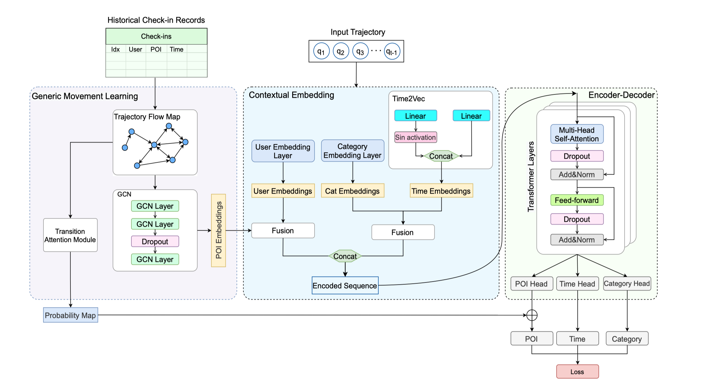
Figure 1. An overview of the GETNext model. (Yang et al., 2022)

4.1. Learning with Trajectory Flow Map

4.1.1. Understanding Trajectory Flow Map

An advanced method entails exploring the details of an attributed weighted directed graph, $G=(V,E,l,w)$. This graph functions as a trajectory flow map and is derived from an extensive set of historical trajectories $S=\{S_{u}^{i}\}_{i\in\mathbb{N},u\in U}$, where:

• Points of Interest (POIs) correspond to the aggregation of nodes $V$.

• For every POI $p\in P$, there are features contained in $l(p)$. These include coordinates $(\text{lat, lon})$, category represented by category, and the frequency eq of occurrence in trajectories in $S$.

• The edges that connect $p_{1}$ and $p_{2}$ in trajectory $S_{u}^{i}$ represented by $(p_{1},p_{2})$ are POI visits in succession.

• Each edge $(p_{1},p_{2})$ has a weight $w(p_{1},p_{2})$, which represents how often it occurs in any trajectory in $S$.

4.1.2. Learning POI Embedding

Vectorized representations of Points of Interest (POIs) are obtained by using Graph Convolution Networks (GCN) with spectral convolution. Through the use of the trajectory flow map, this novel method encodes transition patterns and attributes, allowing for a more thorough comprehension of the overall dynamics of movement at each point of interest.

4.1.3. Deciphering Transition Attention Map

Use of a transition attention map, $\Phi$, allows for a detailed modeling of transition probabilities between POIs. Based on the intrinsic characteristics of the input node, this sophisticated map—which is calculated in the next transformer module—dynamically modifies the conclusions. The recommendation’s results are greatly influenced by the $\Phi$ map, which illustrates the probability of moving from one POI to another.

4.2. Contextual Embedding Module

Personalized next point-of-interest (POI) recommendations are built on top of the Contextual Embedding Module, which combines spatiotemporal contexts with user preferences. Two essential fusion components are included in this module:

4.2.1. POI-User Embeddings Fusion

In order to capture both the general patterns found in POIs and the user-specific behaviors encountered in previous check-in sequences, it is essential to combine user embeddings with POIs. Using a function $\text{fembed}(u)$, we first retrieve the user embedding $e_{u}$ in this case, which is represented as:

(2) $$e_{u}=\text{fembed}(u)\in\mathbb{R}^{\Omega}.$$

User preferences and actions that are subtle are captured in this embedding.

Concatenating the POI embedding $e_{p}$ and the user embedding $e_{u}$ yields the fused embedding $e_{p,u}$, which is then used as follows:

(3) $$e_{p,u}=\sigma(w_{p,u}[e_{p};e_{u}]+b_{p,u})\in\mathbb{R}^{\Omega\times 2},$$

The activation function is indicated by $\sigma$, while the weights and bias are denoted by $w_{p,u}$ and $b_{p,u}$, respectively. To improve the model’s capacity to collect customized recommendations, the concatenated vector $[e_{p};e_{u}]$ combines user attributes with points of interest.

4.2.2. Time-Category Embeddings Fusion

Categorical embeddings of POIs and temporal information recorded by Time2vector are combined in this fusion process. Taking into account the temporal aspect of user behavior, Time2vector efficiently encodes time values. In addition, an embedding layer is used for POI categories concurrently.

The following is the formulation of the fusion equation for time-category embeddings, $e_{c,t}$:

(4) $$e_{c,t}=\sigma(w_{c,t}[e_{t};e_{c}]+b_{c,t})\in\mathbb{R}^{\Psi\times 2},$$

where the learnable weight vector is indicated by $w_{c,t}$, and the bias is represented by $b_{c,t}$. It is easier to integrate temporal and categorical data when $e_{t}$ and $e_{c}$ are concatenated.

The final embedding, $e_{q}$, is the combination of the POI-user and time-category embeddings, and it captures the core of a check-in operation. Each trajectory input consists of a series of check-in embeddings and is represented as $q=\langle p,u,t\rangle$, where POI $p$ is in category $c$. To facilitate precise POI recommendations, the transformer encoder further processes these embeddings to extract complex patterns and insights.

4.3. Transformer Encoder and MLP Decoders

4.3.1. Transformer Encoder

A key element of our architecture is the transformer encoder, which consists of stacked layers with positional encoding and is essential to the next Point of Interest (POI) recommendation procedure. An input tensor $X^{[0]}\in\mathbb{R}^{k\times d}$ is formed by concatenating historical check-in embeddings for each trajectory $S_{u}$, where $d$ is the embedding dimension. Normalization and residual connections are used in conjunction with fully linked networks and multi-head self-attention processes within each layer. The encoder layer produces an output designated as $X^{[l+1]}\in\mathbb{R}^{k\times d}$ after a series of transformations.

(5) $$S=X^{[l]}W_{q}(X^{[l]}W_{k})^{T}\in\mathbb{R}^{k\times k}$$

Using the query and key matrices $W_{q}$ and $W_{k}$ obtained from the encoder output, this equation calculates the similarity matrix $S$.

(6) $$S^{\prime}_{i,j}=\frac{\exp(S_{i,j})}{\sum_{j=1}^{k}\exp(S_{i,j})}$$

The attention weights obtained by softmax normalization of the similarity matrix $S$ are represented by $S^{\prime}_{i,j}$ in this particular case.

(7) $$\text{head}_{1}=S^{\prime}X^{[l]}W_{v}\in\mathbb{R}^{k\times\frac{d}{h}}$$

The output of the first attention head is calculated using this equation.

(8) $$Multihead(X^{[l]})=[head_{1};\ldots;head_{h}]\times W_{o}\in\mathbb{R}^{k\times d}$$

The outputs from each attention head are combined into a single matrix by the multi-head attention mechanism.

(9) $$X^{[l]}_{\text{attn}}=\text{LayerNorm}(X^{[l]}+\text{Multihead}(X^{[l]}))$$

The application of layer normalization to the multi-head attention output and the sum of the input tensor is represented by this equation.

(10) $$X^{[l]}_{\text{FC}}=\text{ReLU}(W_{1}X^{[l]}_{\text{attn}}+b_{1})W_{2}+b_{2}\in\mathbb{R}^{k\times d}$$

The layer normalization output is subjected to the feed-forward neural network modification.

(11) $$X^{[l+1]}=\text{LayerNorm}(X^{[l]}_{\text{attn}}+X^{[l]}_{\text{FC}})\in\mathbb{R}^{k\times d}$$

By applying layer normalization to the total of the output from the feed-forward network and the attention mechanism, the transformer encoder layer’s final output is obtained.

4.3.2. MLP Decoders

A key component in predicting the next POI, visiting time, and POI category is the multi-layer perceptron (MLP) decoders, which take input from the transformer encoder output. There are three different MLP heads that carry out these predictions. Combining the output from the POI head with the transition attention map yields the final recommendation. In other words, the time head models the intervals between check-ins, while the category head controls the forecasts for the following POI.

(12) $$\hat{Y}_{\text{poi}}=X^{[l^{*}]}W_{\text{poi}}+b_{\text{poi}}$$

Using the encoder output as a basis, this formula determines the anticipated next POI.

(13) $$\hat{Y}_{\text{time}}=X^{[l^{*}]}W_{\text{time}}+b_{\text{time}}$$

The encoder output is used in this calculation to determine the estimated visit time.

(14) $$\hat{Y}_{\text{cat}}=X^{[l^{*}]}W_{\text{cat}}+b_{\text{cat}}$$

Based on the encoder output, this equation indicates the next POI category that is predicted.

4.3.3. Loss

The most important component in the model’s training process is the loss function, which takes into account several aspects of prediction accuracy. It combines different variables to offer an all-encompassing assessment, guaranteeing strong performance on a range of prediction tasks. In particular, the loss function includes cross entropy for both the temporal prediction and the point of interest (POI) category predictions, as well as mean squared error (MSE) for temporal prediction. Taken together, these metrics assess how well the model represents temporal dynamics and classifies points of interest and the categories that go along with them.

A deliberate amplification method is used to handle the complexities of temporal prediction and preserve balanced gradients throughout optimization. Notably, in the final loss computation, the contribution of the temporal loss component is multiplied by a factor of 10. This purposeful modification seeks to ensure that temporal dynamics receive the proper attention in the training regimen and to lessen the possible dominance of other loss components.

The final loss function can be mathematically represented by the following equation:

(15) $$L_{\text{final}}=L_{\text{poi}}+10\times L_{\text{time}}+L_{\text{cat}}$$

In this case, the individual loss contributions resulting from POI prediction, temporal prediction, and POI category prediction are denoted by the variables $L_{\text{poi}}$, $L_{\text{time}}$, and $L_{\text{cat}}$. The loss function offers a comprehensive assessment of model performance by combining these elements into a single framework and directing the optimization process in the direction of improved prediction accuracy and generalization capacity.

5. Experiment

5.1. Dataset

As part of our experiment, we carefully examined the FourSquare-NYC public dataset, which is an extensive collection of urban check-in patterns in New York City that was carefully collected and described by Dingqi et al. (Yang et al., 2014). Covering the busy streets of April 2012 to the quiet streets of February 2013, this dataset captures a variety of user interactions within the dynamic cityscape. Every entry in this list represents an assembly of essential data, such as the user’s name, the point of interest (POI) that was visited, the particular category that the POI falls under, the exact GPS coordinates indicating its location, and the timestamp indicating the interaction.

We started the process of data refining in order to obtain more sophisticated insights through eliminating users who had very few check-ins in the past, leaving only those who had an important record of at least ten actions that were recorded. In a similar manner, we removed POIs with less than 10 check-in records from the dataset to make sure our analysis was supported by reliable and significant data points.

After a thorough curation process, we changed our focus to segmenting users’ check-in behaviors into coherent paths. A detailed picture of users’ engagement patterns across time was provided by the division of these trajectories, which were distinguished by their temporal continuity and spatial diversity, into discrete segments separated by 24 hours. We acknowledged the natural fluctuations in check-in rates, therefore in order to maintain statistical integrity, we carefully examined trajectories where there was only one check-in. These were identified as outliers and removed from the dataset.

After carefully priming and preparing our dataset, we divided it into several subgroups for testing, validation, and training. The trajectory flow map—a fundamental artifact of our analytical journey—was carefully developed from the first 80% of check-ins designated for training, the next 10% for validation, and the last 10% sacrosanct for testing.

One of the most important components of our technique was the strict exclusion criteria we used for evaluation, which made sure that any people or items of interest that we had not experienced in the training phase were not included in the performance assessment. As a result, our predictive models were protected from bias and overfitting, and a more sophisticated comprehension of their actual ability to predict was developed.

Significant statistics from the dataset are shown in Table 1.

Table 1. Dataset Statistics

user	poi	cat	checkin	trajectory
1,075	5,099	318	104,074	14,160

Table 2. Experimental Results

$\alpha$	$\beta$	Acc@1	Acc@5	Acc@10	Acc@20	MRR
GETNext		0.6177	0.8477	0.9051	0.9455	0.7196
0.33	0.33	0.5856	0.8468	0.8946	0.9468	0.6984
	0.50	0.5949	0.8622	0.9108	0.9470	0.7115
	0.67	0.5995	0.8360	0.8889	0.9294	0.7030
0.50	0.33	0.5268	0.7951	0.8586	0.9174	0.6481
	0.50	0.5615	0.8174	0.8799	0.9323	0.6769
	0.67	0.5721	0.8233	0.8792	0.9227	0.6820
0.67	0.33	0.5346	0.7939	0.8534	0.9183	0.6485
	0.50	0.5445	0.8228	0.8858	0.9328	0.6679
	0.67	0.5988	0.8527	0.9110	0.9500	0.7147

Note: The GETNext model’s output is shown in the first row. The performance metrics for various combinations of $\alpha$ and $\beta$ parameters are shown in the subsequent rows. The exact values of $\alpha$ and $\beta$ for each matching row are shown in the first two columns, respectively.

5.2. Evaluation Metrics

We use advanced metrics to assess the performance of our recommendation system during the evaluation process. In particular, we explore two well-known metrics in the field of recommender systems: Mean Reciprocal Rank (MRR) and Accuracy@k (Acc@k). These metrics give important information about how well the model is performing, including how well it can recommend points of interest (POIs) to users.

To determine whether the real POI is among the top-k recommended POIs, the Accuracy@k measure is used as an indicator of accuracy. It basically assesses how well the algorithm identified pertinent POIs from a given set of recommendations. This indicator is especially helpful for assessing how accurately and efficiently the system provides users with ideas that are relevant to their needs. Formally, the Accuracy@k is determined in this way:

$$\text{Acc@k}=\frac{1}{m}\sum_{i=1}^{m}1(\text{rank}\leq k)$$

In this case, the total number of samples or trajectories in our dataset is indicated by $m$. To indicate whether the rank of the real POI in the sorted list of recommendations is in the top k spots, the ranking indicator function $1$ is utilized. The function produces $1$ if the condition is met; $0$ is produced otherwise.

The rating of the right recommendation inside the sorted list is taken into account by the Mean Reciprocal Rank (MRR), which provides a more comprehensive viewpoint. In contrast to Accuracy@k, which handles the top-k recommendations as an unordered list, MRR considers the exact location of the right recommendation within the ordered list. This statistic plays a crucial role in evaluating how well the system ranks and prioritizes pertinent points of interest. This is how the MRR is determined:

$$\text{MRR}=\frac{1}{m}\sum_{i=1}^{m}\frac{1}{\text{rank}}$$

The real next point of interest in the sorted list is indicated by the symbol rank in this case. A thorough assessment of the system’s ranking performance is offered by the MRR, which is calculated by averaging the reciprocals of the ranks over all samples.

Better performance is essentially indicated by higher values of Accuracy@k and MRR, which show how well the system can appropriately recommend pertinent POIs to users. We can refine and optimize our recommendation system to increase user satisfaction and engagement by using these metrics, which are vital tools for evaluating the efficacy and usefulness of the system.

5.3. Results

We have conducted a number of well designed experiments that have contributed significantly to our understanding of the complex dynamics of our model and marked our journey through the dataset. Despite the trials, the fundamental pillars of our study, denoted by the mysterious variables $\alpha$ and $\beta$, as stated in equation 1, held firm. Our technique stayed largely unchanged across a resolute span of 20 epochs, which allowed our comparison study to remain coherent.

As we carefully examined the temporal structure of our dataset, an important distinction became apparent. Check-ins sought solace in two discrete temporal domains—the recent and the past—amid the complex pattern of temporal dynamics. Those who were recorded in the history of the previous three months were labeled as recent. On the other hand, those who came before this point in time were relegated to the past.

Table 2 presents the empirical evidence that we gathered during our extensive experimentation. The highlights of our model’s performance are arranged in columns and rows. By applying a critical eye to statistical analysis, we compared the many combinations of $\alpha$ and $\beta$ and uncovered the complex dynamics between these variables.

It is clear that tests considering the quantity of users who generated check-in records and the time passed since check-in data were generated outperformed the baseline in a range of scenarios. The scenario would have been different if the model had been trained for more epochs, even though baseline has the best Acc@1.

6. Conclusion

We set out to redefine the concept of popularity assigned to a point-of-interest (POI) within the constraints of this research in order to further the area of POI recommendation systems. Our work is completed by integrating this new idea into GETNext, a unique graph-based learning model designed for POI recommendation tasks on a global graph structure. Elaborating on the complex relationship between the model’s effectiveness and the subtle interactions between two important parameters, $\alpha$ and $\beta$, as shown by equation 1, we approached this task with great care. We thoroughly examined the model’s performance dynamics over a range of $\alpha$ and $\beta$ values using a stringent set of experiments on an extensive real-world dataset, revealing a wealth of information about the complex behavior of the recommendation system. But our investigation doesn’t finish here; rather, it’s just the beginning of a longer journey to learn more about the time aspect of POI recommendation. We will next attempt to understand the complex time dynamics at work, determine the time influence on other variables, and clarify how the more general travel patterns change with the seasons. A greater comprehension of the fundamental processes guiding POI recommendation systems is anticipated to be revealed by these upcoming studies, opening the door to more reliable and contextually sensitive recommendation frameworks.

References

- (1)
- Cheng et al. (2013) Chen Cheng, Haiqin Yang, Michael R. Lyu, and Irwin King. 2013. Where you like to go next: Successive point-of-interest recommendation. In Twenty-Third international joint conference on Artificial Intelligence.
- Feng et al. (2018) Jie Feng, Yong Li, Chao Zhang, Funing Sun, Fanchao Meng, Ang Guo, and Depeng Jin. 2018. DeepMove: Predicting Human Mobility with Attentional Recurrent Networks. 1459–1468. https://doi.org/10.1145/3178876.3186058
- Feng et al. (2020) Shanshan Feng, Lucas Vinh Tran, Gao Cong, Lisi Chen, Jing Li, and Fan Li. 2020. HME: A hyperbolic metric embedding approach for next-poi recommendation. In Proceedings of the 43rd International ACM SIGIR Conference on research and development in information retrieval. 1429–1438.
- Li et al. (2021) Yang Li, Tong Chen, Yadan Luo, Hongzhi Yin, and Zi Huang. 2021. Discovering Collaborative Signals for Next POI Recommendation with Iterative Seq2Graph Augmentation. In Proceedings of the Thirtieth International Joint Conference on Artificial Intelligence, IJCAI-21, Zhi-Hua Zhou (Ed.). International Joint Conferences on Artificial Intelligence Organization, 1491–1497. https://doi.org/10.24963/ijcai.2021/206 Main Track.
- Liu et al. (2016) Qiang Liu, Shu Wu, Liang Wang, and Tieniu Tan. 2016. Predicting the next location: A recurrent model with spatial and temporal contexts. In Proceedings of the AAAI conference on artificial intelligence, Vol. 30.
- Rendle et al. (2010) Steffen Rendle, Christoph Freudenthaler, and Lars Schmidt-Thieme. 2010. Factorizing personalized markov chains for next-basket recommendation. In Proceedings of the 19th international conference on World wide web. 811–820.
- Sun et al. (2020) Ke Sun, Tieyun Qian, Tong Chen, Yile Liang, Nguyen Hung, and Hongzhi Yin. 2020. Where to Go Next: Modeling Long- and Short-Term User Preferences for Point-of-Interest Recommendation. Proceedings of the AAAI Conference on Artificial Intelligence 34 (04 2020), 214–221. https://doi.org/10.1609/aaai.v34i01.5353
- Wu et al. (2019) Yuxia Wu, Ke Li, Guoshuai Zhao, and Xueming Qian. 2019. Long- and Short-term Preference Learning for Next POI Recommendation. 2301–2304. https://doi.org/10.1145/3357384.3358171
- Wu et al. (2020) Yuxia Wu, Ke Li, Guoshuai Zhao, and Xueming Qian. 2020. Personalized long-and short-term preference learning for next POI recommendation. IEEE Transactions on Knowledge and Data Engineering 34, 4 (April 2020), 1944–1957.
- Yang et al. (2014) Dingqi Yang, Daqing Zhang, Vincent W. Zheng, and Zhiyong Yu. 2014. Modeling user activity preference by leveraging user spatial temporal characteristics in LBSNs. IEEE Transactions on Systems, Man, and Cybernetics: Systems 45, 1 (January 2014), 129–142.
- Yang et al. (2022) Song Yang, Jiamou Liu, and Kaiqi Zhao. 2022. GETNext: trajectory flow map enhanced transformer for next POI recommendation. In Proceedings of the 45th International ACM SIGIR Conference on research and development in information retrieval. 1144–1153.
- Yuan et al. (2014) Quan Yuan, Gao Cong, and Aixin Sun. 2014. Graph-based Point-of-interest Recommendation with Geographical and Temporal Influences. CIKM 2014 - Proceedings of the 2014 ACM International Conference on Information and Knowledge Management, 659–668. https://doi.org/10.1145/2661829.2661983
- Zhang et al. (2014) Jia-Dong Zhang, Chi-Yin Chow, and Yanhua Li. 2014. LORE: exploiting sequential influence for location recommendations (SIGSPATIAL ’14). Association for Computing Machinery, New York, NY, USA, 103–112. https://doi.org/10.1145/2666310.2666400
- Zhao et al. (2020) Kangzhi Zhao, Yong Zhang, Hongzhi Yin, Jin Wang, Kai Zheng, Xiaofang Zhou, and Chunxiao Xing. 2020. Discovering Subsequence Patterns for Next POI Recommendation. In Proceedings of the Twenty-Ninth International Joint Conference on Artificial Intelligence, IJCAI-20, Christian Bessiere (Ed.). International Joint Conferences on Artificial Intelligence Organization, 3216–3222. https://doi.org/10.24963/ijcai.2020/445 Main track.
- Zhao et al. (2019) Pengpeng Zhao, Haifeng Zhu, Yanchi Liu, Jiajie Xu, Zhixu Li, Fuzhen Zhuang, Victor S. Sheng, and Xiaofang Zhou. 2019. Where to Go Next: A Spatio-Temporal Gated Network for Next POI Recommendation. Proceedings of the AAAI Conference on Artificial Intelligence 33, 01 (Jul. 2019), 5877–5884. https://doi.org/10.1609/aaai.v33i01.33015877