On the power of data augmentation for head pose estimation

Abstract

Deep learning has been impressively successful in the last decade in predicting human head poses from monocular images. For in-the-wild inputs, the research community has predominantly relied on a single training set of semi-synthetic nature. This paper suggest the combination of different flavors of synthetic data in order to achieve better generalization to natural images. Moreover, additional expansion of the data volume using traditional out-of-plane rotation synthesis is considered. Together with a novel combination of losses and a network architecture with a standard feature-extractor, a competitive model is obtained, both in accuracy and efficiency, which allows full 6 DoF pose estimation in practical real-time applications.

1 Introduction

Human head pose estimation (HPE) is an important task in many application e.g. in the automotive sector or in entertainment products. The specific problem in this paper is monocular head pose estimation for in-the-wild scenarios, i.e. we are given a crop of a face as input to our computer vision system from which it estimates the face orientation and optionally location and size. Closely related is the task of face alignment where a mathematical description of a face is inferred, e.g. as landmarks or a full 3D reconstruction. These tasks are particularly challenging due to the diversity and non-rigid nature of faces. However, in recent years deep learning methods have been very successful at it [1]. In HPE, the current state of the art achieves errors of ca. $3$ (MAE) or $5^{\circ}$ (geodesic) [2, 3].

The main interest in this work lies in devising a simple, efficient and effective HPE model. Because the margin for model size and complexity is thus limited, choice of the training data is a knob left to turn freely. Therefore the goal of this paper is also to elucidate the impact of this choice. Before introducing custom datasets later we shall now briefly review the related literature. For in-the-wild HPE we recognize two datasets as de-facto standard: AFLW2000-3D and 300W-LP from the same authors [4]. AFLW2000-3D, serving as test set, consists of 2000 images labeled with 6 DoF poses, parameters for reconstructing a 3D mesh, as well as landmarks. The images are challenging due to occlusion, extreme poses, varying illumination and so on. 300W-LP similarly consists ca. 61 thousand labeled images. It was constructed by augmenting a smaller set of faces with out-of-plane rotations and generally serves as training set. Some authors chose to expand this data [5] further with fine-grained movements, or employ a face swapping augmentation [6]. However the effect of doing so is rarely considered in isolation. HPE utilizing fully synthetic images has also been considered. Specifically [7, 8, 9] consider rather a laboratory setting with only a small number of individuals on the basis of the SynHead dataset for training [7]. For this work, I included a different fully synthetic dataset, Face Synthetics [10], which provides labeled images of $10^{5}$ randomized individuals.

Regarding mathematical models for HPE, a baseline may consist of a learned feature extractor, such as a convolutional neural network, and final linear layers which, after some simple transformation output orientation, position, size and so on. Such a network could be trained with losses such as L1 or L2 penalizing the errors from the known ground truths. Various rotation representations have been proposed [11, 12, 2]. Other works propose more sophisticated model structures and loss calculations [6, 3, 13]. Others employ complex training schedules switching between different losses dynamically [5]. Yet others construct multi-task networks [14] to leverage commonalities between 3D HPE and 2D landmark prediction. However, even with conceptually simply methods and small networks it is possible to obtain excellent results as shown in [2].

The contributions of this paper are:

• Proposing a novel head pose estimation network with improved accuracy over the current state of the art.

• Introducing extended training sets and novel combinations of data augmentations and losses.

• Ablation studies highlighting the effectiveness of additional data and various model ingredients.

• Considering practical aspects, specifically noise-resistance and uncertainty estimation.

The model was integrated into the FOSS OpenTrack , and will therefore be referred to as OpNet. The full source code for training and eval is available on github .

2 Methods

This section explains the construction of the model.

2.1 Prediction model

The model architecture consists of a feature extraction backbone, global pooling, $50\%$ dropout, and a linear layer per prediction head. The raw features of each head are mapped to a final predicted quantity, respectively.

As input, the model takes a $129\times 129$ monochrome face crop. The motivation for monochrome inputs is to guarantee invariance to hue changes in the local illumination conditions.

The literature provides a rich selection of feature extraction networks developed for image classification. Several of them promise favorable runtime performance [15, 16, 17, 18, 19, 20]. We will consider only ResNet18 [15] and MobileNetV1 [18] because I found them to perform as well or better than more recent proposals.

To enable full 6 DoF tracking, and to enable learning from landmark-only annotations, the model has the following outputs:

• rotation quaternion,

• 2D position and head size,

• shape parameters of a deformable face model,

• head bounding box,

• rotation uncertainty,

• position and size uncertainty.

The orientation is described by a Rotation quaternion, represented by a normalized four-dimensional vector. Note that the quaternions $q$ and $-q$ represent the same orientation. Results were better if this ambiguity was avoided and the network was biased toward zero rotation. Hence our quaternion is formed by $q=q^{\prime}/||q^{\prime}||,q^{\prime}=iz_{0}+jz_{1}+kz_{2}+\mathit{smoothclip}(z_{3})$, where $i$,$j$,$k$ is the imaginary basis, $\mathit{smoothclip}(x)=\mathit{ELU}(x)+1$ maps $\mathbb{R}$ to $\mathbb{R}^{+}$ and $\mathit{ELU}$ is the ELU activation function [21]. For $\pm 180^{\circ}$ range there are better representations than quaternions. For our application with angles up to $\pm 90^{\circ}$, this is less of a problem [2].

2D position and size are both estimated in image space, normalized to $[-1,1]$. The 2D position is taken identically from the respective linear layer. The size feature is passed through our $\mathit{smoothclip}$ function in order to guarantee a positive value.

Shape parameters and in particular the derived 3D landmarks are intended for training on datasets which provide landmarks but no pose. We will see that incorporating landmarks boosts the accuracy of the model even when pose labels are available. Following the literature [4, 22, 5, 6, 13], landmark estimation is based on the Basel Face Model (BFM) [23]. Its geometry is defined by a base shape in terms of vertices and triangles, supplemented by a basis of deformation vectors describing offsets from the base vertices. Hence varying head shapes and facial expressions can be obtained by adding a linear combination of the deformation vectors to the base vertices. Our network, like e.g. [5], predicts coefficients for a subset of 50 of those vectors. The mesh is transformed into the image plane by scale, rotation and translation according to the pose prediction. Note that orthographic projection is assumed where the z-axis points into the image plane. Hence no further camera transform is needed. Landmarks are constructed by taking 68 vertices from the mesh as in [4, 5], adhering to the MultiPIE-68 landmark markup [24, 25].

The bounding box prediction is present for continuously tracking the face. Thus we can continuously update a crop from a video feed in the manner of the demo application from [5]. I added the explicit box estimate for achieving consistency of the updated crop with the crop at train time and flexibility to allow any cropping scheme. The box is parameterized by center $(x,y)$ and size $(w,h)$, where $x=z_{0},y=z_{1},w=\mathit{smoothclip}(z_{2}),h=\mathit{smoothclip}(z_{3})$ with features $z_{i}$.

Rotation uncertainty, and knowledge of the uncertainty of a measurement in general, are useful for Bayesian filtering by Kalman filters [26] for example. We will see that adding the uncertainty estimates also boosts the model performance. For simplicity, I chose to predict only aleathoric (data) uncertainty which is implemented by adding variance parameters as outputs [27, 28]. Essentially. the network is trained to predict the magnitude of label noise.

Deep learning with rotational uncertainty is unfortunately not straight forward. Representing uncertainty by probability densities on $SO(3)$, the space of rotations, is considered in [29, 30, 31, 32]. A popular choice is the Matrix Fisher distribution [33] which has been considered for HPE in [34]. The authors of [35] on the other hand derive an uncertainty estimate directly from their rotation representation. Drawbacks of these methods are numerical challenges, requiring matrix factorizations and/or normalization constants which cannot be expressed in closed form.

In this paper the uncertainty is therefore represented by a Normal distribution in the tangent space $\mathfrak{so}(3)$. Essentially $\mathfrak{so}(3)$ encodes differences from the current orientation in terms of 3D rotation vectors. To eliminate redundancy, the center of the distribution is fixed at zero. Note that this is not a distribution on $SO(3)$. However, it asymptotically approximates one for decreasing variance [36, 37, 29].

It follows that we need a covariance matrix $\bf\Sigma$, which must be constructed to ensure positive definiteness. Fortunately this is easy. The network outputs a lower triangular matrix $M\in\mathbb{R}^{3\times 3}$ filled with six features from the linear layer. Then the covariance matrix is set to $\bf\Sigma=MM^{T}+\epsilon\bf I$, where ^T means transpose and $\bf I$ is the identity matrix. This is akin to a Cholesky decomposition but the diagonals of $\bf M$ do not need to be positive and the addition of $\bf I$ scaled with a small constant ensures positivity. Note that $\bf MM^{T}$ is positive semi-definite.

Position and size uncertainty is modeled by a 3D multi-variate Normal distribution for the triplet combining 2D position and head size. Its covariance matrix is constructed in the same way as for the rotation vectors.

2.2 Losses

The training procedure minimizes the sum of individual losses which correspond roughly to the prediction outputs. Learning mean and variance parameters, $\mu,\sigma$ is commonly done by minimizing the negative log likelihood (NLL) $-\log p(y|\mu(x),\sigma(x))$ over some dataset consisting of many input-output tuples $(x,y)$, $p$ denoting the probability density [27, 28]. Naive approaches have often been reported as unstable [38, 39]. As remedy, an initial period where the variance is fixed was suggested. For historical reasons my model is instead trained with a combination of traditional regression losses and NLLs. For "symmetry" reasons I employ NLLs even for shape parameters, bounding box and landmarks, in case of which variances are learned as auxiliary parameters independent of the inputs. In the following, estimated quantities will be marked with hat $\hat{.}$ and ground truth without.

The losses for Rotation are defined by:

$$L_{rot}(\hat{q},q) =1-|\hat{q}\cdot q|^{2}$$ (1)

$$\textit{NLL}_{rot}(\hat{q},q,{\bf\hat{\Sigma}}_{rot}) =-\log f(\textit{Im}\log(\hat{q}^{-1}q)|0,{\bf\hat{\Sigma}}_{rot})\text{,}$$ (2)

where $f$ refers to the density of the Normal distribution, $\cdot$ is the vector inner product, $\log$ applied to the quaternion returns an imaginary quaternion containing the rotation vector (axis times magnitude), and Im extracts the imaginary part as 3d vector. Note that $|\hat{q}\cdot q|\in[0,1]$ since the $q$’s are unit quaternions. See also [40] for various metrics and mathematical details on $SO(3)$.

Consider position and size again as concatenated into a 3d vector $p$. The employed losses are L2 and NLL with the Normal distribution with variance ${\bf\hat{\Sigma}}_{p}$. Thus we can write:

$$L_{p}(\hat{p},p) =||p-\hat{p}||^{2}$$ (3)

$$\textit{NLL}_{p}(\hat{p},p,{\bf\Sigma}_{p}) =-\log f(p|\hat{p},{\bf\Sigma}_{p})\text{.}$$ (4)

The shape parameters, denoted $\phi_{i}$, are assumed to be distributed independently normal. This simplifies the covariance to a diagonal matrix ${\bf\hat{\Sigma}}_{shp}=\textit{diag}(\sigma_{1},\sigma_{2},\dots)$, where, as stated, $\sigma_{i}$’s are learned independent of the input image. The corresponding losses are the L2 loss $L_{\phi}(\hat{\phi},\phi)$ and NLL with Normal distribution $\textit{NLL}_{\phi}(\hat{\phi},\phi,{\bf\hat{\Sigma}}_{\phi})$ which are defined analogously to Eqs. (3) and (4), and omitted for brevity.

For landmarks I found the L1 loss to work well. The corresponding NLL is based on the Laplace distribution. Again, statistical independence is assumed. Then the total loss decomposes into sums over coordinate-wise contributions. Moreover, I found it useful to apply weights $w_{i}$ to different parts of the face. Thus, the losses are defined by

$$L_{\xi}(\hat{\xi},\xi) =\sum_{i}w_{i}|\xi_{i}-\hat{\xi}_{i}|$$ (5)

$$\textit{NLL}_{\xi}(\hat{\xi},\xi,{\bf\hat{\Sigma}}_{\xi}) =-\sum_{i}w_{i}\log f_{\mathit{Laplace}}(\xi_{i}|\hat{\xi}_{i},\hat{\sigma}_{\xi,i})\text{,}$$ (6)

where $i$ runs over the 68 $\times$ 3 spatial landmark coordinates. If only x and y coordinates are available, then the summation runs only over those.

The bounding box is trained like the shape parameters using L2 loss $L_{bb}$ and Normal $\textit{NLL}_{bb}$. Input to those losses are the box corner coordinates, assuming independence.

In order to encourage the network to output nearly unit quaternions I added $L_{norm}(\hat{q}^{\prime})=|1-|\hat{q}^{\prime}||^{2}$. Where $\hat{q}^{\prime}$ is the unnormalized quaternion.

At last we can define the total loss $L$ by

$$L=1/B( \alpha_{rot}L_{rot}+\alpha_{p}L_{p}+\alpha_{\phi}L_{\phi}+\alpha_{\xi}L_{\xi}+\alpha_{bb}L_{bb}+\alpha_{norm}L_{norm}$$ (7)

$$\beta_{total}[\beta_{rot}\textit{NLL}_{rot}+\beta_{p}\textit{NLL}_{p}+\beta_{\phi}\textit{NLL}_{\phi}+\beta_{\xi}\textit{NLL}_{\xi}+\beta_{bb}\textit{NLL}_{bb}])\text{,}$$ (8)

with weighting factors $\alpha_{.}$ and $\beta_{.}$ and batch size $B$.

2.3 Augmentations

I apply translation, rotation, mirror, scale and intensity augmentation. Input to this pipeline are the source image, not necessarily cropped, a 2D facial bounding box (BB), and remaining labels which are consistently geometrically transformed. In principle, a random square region of interest (ROI) is generate from the BB extending its shortest side, scaling, rotating, and offsetting it. Then the ROI is resampled creating the input crop matching the input resolution of the network. In practice, these steps are implemented using an affine warp transformation. The scale factor is sampled from $\mathcal{N}(1.1,0.1)$ and clipped to $[1.1-0.5,1.1+0.5]$. The rotation angle is sampled from a uniform distribution up to $30^{\circ}$. The offset is also drawn from a clipped Gaussian and so that a minimum of $70\%$ of the original BB is still visible. The final geometric augmentations are horizontal mirroring with probabiliy $1/2$ and $90^{\circ}$ rotation with probability $1/100$. The BB is regenerated by taking the BB around the transformed corner points.

Next, image intensity augmentation from the Kornia package are applied. From Equalize, Posterize, Gamma, Contrast, Brightness, and Blur, four are picked and applied with small probabilities, up to $1/10$ chance. Afterwards Gaussian noise is randomly added twice, once with probability $p=1/2$ and $\sigma=4$ and secondly with $p=0.1$ and $\sigma=16$, w.r.t a maximum image intensity of $255$. I deliberately add noise frequently with the intent to generalize to low-light conditions.

2.4 Implementation Details

The network is trained with the ADAM optimizer [41] for $N=15$M samples with a maximum learning (LR) rate of $10^{-3}$. The LR ramps-up for $N/20$ samples and decreases in a step to $1/10$th after $N/2$ samples. After $2/3N$ samples, stochastic weight averaging [42] is enabled. Training time is $4$ to $5$h on a Ryzen 9 5900X with a GeForce 3060 TI.

As explained below in Sec. 3, multiple datasets are considered for training. Combining them is done via simple random draws. First a dataset is picked with a certain frequency reported in Sec. 4, and then a sample is picked from there with equal chances. Sampling is always with replacement.

Regarding the landmark weights, I do not train the eye centers - top and bottom, 8 point in total - since good samples with closed eyes are scarce. Hence weights $w_{i}$ are set to zero for corresponding landmarks. The loss weights are $\alpha_{rot}=1$,$\alpha_{p}=1$,$\alpha_{\phi}=0.01$,$\alpha_{\xi}=1$,$\alpha_{bb}=0.01$, $\alpha_{norm}=10^{-6}$, $\beta_{total}=0.01$ to bring the NLL range to the same order of magnitude as the other losses, $\beta_{rot}=1.$,$\beta_{p}=1.$,$\beta_{\phi}=0.01$,$\beta_{\xi}=1$ and $\beta_{bb}=0.01$. If a loss is infeasible due to missing labels, in particular when only landmark annotations are present, then their weights $\alpha_{.}$, $\beta_{.}$ are in effect set to zero instead.

3 Datasets

The model is evaluated on AFLW2000-3D introduced in Sec. 1. I follow the standard protocol in [43] and remove the 30 samples with yaw, pitch or roll angles larger than $99^{\circ}$. Following wide spread use throughout the literature, initial experiments were conducted with the 300W-LP dataset [4] for training.

3.1 Extended 300W-LP Reproduction

When trained on 300W-LP [4], my networks showed small but noticeable systematic pose deflections depending on whether the subjects eyes are closed or not (unpublished). Perhaps this is related to the lack of images with closed eyes. Moreover, illumination conditions in 300W-LP are fairly uniform.

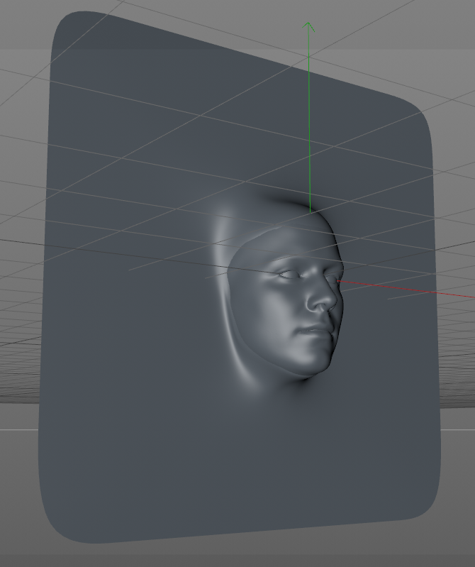
Figure 4: The underlying mesh for rendering images with out-of-plane rotations.

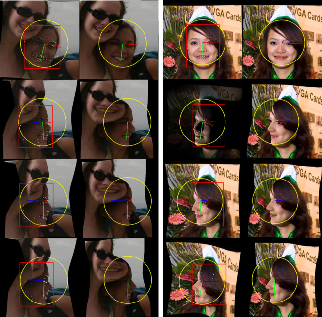
Figure 5: Example frames of the extended 300W-LP dataset. Left and right panel show difference subjects. Per panel, left column: new, right column: 300W-LP.

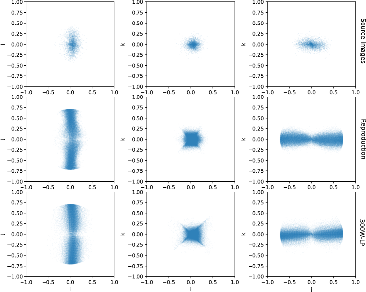
Figure 8: Rotation distribution of the expansion by in-plane rotations. The plots show projections of the quaternion components of the rotation annotations. Every point represents a sample in the respective dataset. Top row: original without expansion. Middle: my reproduction. Bottom: 300W-LP.

This motivated the creation of a new dataset following the original [4] to address the shortcomings with the eyes and illumination. However, this relates only to the out-of-plane rotation synthesis. I used the 300W-LP source images and BFM parameters. Let’s consider the key ingredients. Firstly, the 3D face model. On the basis of same facial region of the BFM as in [5], a smooth transition to a background plane was modeled. The resulting mesh is shown in the Appendix Fig 4. The deformation basis was extended to the new vertices by copying the vectors from the closest BFM vertex and attenuating them by a distance-dependent decay factor. To the original basis new shapes with a closed eyes were added. Given an input image, a depth profile is imposed on the background plane according to a monocular depth estimate. This is performed by an off-the-shelf MiDaS model [44, 45]. Then, as in [4], a new image is generated by projecting the original image onto the 3D mesh, rotating the face together with the left or right half of the background, smoothly blending between transformed and pristine parts, and rendering the result. In addition to unlit renderings, I also generate faces lit from the side by a directional light source with probability $1/1000$. Closed eyes are sampled with probability $1/2$. The Appendix contains comparisons with 300W-LP in the image panel Fig. 5 and the scatter plots of rotation distributions in Fig. 8. It shall be said that while they appear to help, the novel eye and illumination additions are far from perfect. The eye regions suffer from small misalignment errors (in particular in Sec. 3.2) and the illumination suffers from shadow-mapping artifacts and generally does not look particularly realistic. The source code is available in a separate repository .

3.2 WFLW & LaPa Large Pose Extension

This section covers further expansion of the training data. To the best of my knowledge, more suitable in-the-wild images annotated with BFM parameters are hardly readily available. As an improvised solution, 2D landmark annotations were leveraged. Perfect labels are thereby not the goal but that the network could learn from relative differences after 300W-LP-style out-of-plane rotation synthesis. The idea is to fit 3D landmarks of the BFM to the 2D annotations which was partially inspired by face-alignment methods [46, 47, 47, 48] based on the FLAME head-model [49] which incorporate guidance by 2D landmarks in addition to photometric fitting and other techniques. Naively fitting 2D annotations is not feasible because landmarks on only the visible side of the face are insufficient to uniquely identify a plausible 3D reconstruction. However, for this paper good enough results could be achieved by incorporating initial guesses and priors from estimation networks as explained in the following:

First a pose-estimator ensemble was trained on the 300W-LP reproduction, following the rest of this paper. Then the input images were pseudo-labeled with pose and shape parameters as reasonable priors. Furthermore, a Gaussian Mixture was trained on the shape parameter distribution of 300W-LP. Finally, for each image the BFM was fitted separately by solving a standard minimization problem for the sum of several losses: landmark error, rotation error from the pseudo-labels, NLL of the gaussian mixture, as well as soft constraints for quaternion normalization and head-size positivity. The landmark losses were weighted depending on the rotation prior so that mostly visible landmarks would be fitted. As the very last steps, failed fits were filtered, the dataset manually curated, and the rotation expansion from Sec. 3.1 applied.

The procedure was applied to WFLW [50] and LaPa [51]. Appealing for this paper, they consist of facial images of a large variety of individuals, poses, and occlusions. WFLW comes with $7.5\cdot 10^{3}$ training images with 98 manually annotated landmarks. The landmarks were converted to 68 points by interpolation. LaPa contains ca. $1.8\cdot 10^{4}$ images annotated with 106 points. However, the latter includes images from 300W-LP which were excluded due to the overlap. The remaining images are from Megaface [52]. Ultimately, there were $4942$ images from LaPa expanded to ca. $7.7\cdot 10^{4}$, and $1554$ images from WFLW expanded to ca. $2.2\cdot 10^{4}$. The created datasets are provided via the github repository. The Appendix contains Figs. 6 and 7 with sample images.

3.3 Face Synthetics

The Face Synthetics dataset [10] consists of $10^{5}$ fully synthetic, photorealistically rendered human heads, annotated with segmentation masks and 3D landmarks. The subjects are composed of randomly sampled face shape, hair style, accessories, skin color, superimposed on a variety of backgrounds. Thus the annotations are perfect and distortions from 300W-LP-style out-of-plane rotations are absent. The authors unfortunately provide only the 3D landmarks and of those only the x and y coordinates. Hence only the corresponding landmark losses $L_{\xi}$ and $\textit{NLL}_{\xi}$ are enabled.

3.4 Face Bounding Box

Cropping is commonly based on the bounding box around the ground truth facial landmarks [13, 5]. However, it might be beneficial to see more of the subjects head. This lead me to the following approach. When pose and BFM parameters are available, the BB encompasses the reconstructed facial section of the BFM, the same as in Sec. 3.1 or [5]. Face Synthetics on the other hand, provides segmentation masks. Hence, there the bounding box encompasses pixels marked as "face" and "nose". Samples where a side length is less than 32 pixels are filtered out. The result is that more of the forehead is included, visually more similar to manual annotation, e.g. from [53].

4 Results

This section covers the accuracy of the model (OpNet) and some ablation experiments. The training is non-deterministic. Therefore evaluations were performed on five different networks and the metrics were averaged. Reported are the average absolute errors of Euler angles, the mean of those (MAE), as well as the average of the geodesic errors $||\textit{Im}\log(\hat{q}^{-1}q)||$. The largest observed standard error of the sample mean was $0.03^{\circ}$ among all experiments, rounded up. To avoid clutter I will only give this conservative estimate.

The baseline (BL) was trained on the combination of custom large pose expansions of 300W-LP, WFLW and LaPa as explained in Sec. 3.1 and 3.2 with sampling probabilities $50\%$, $33\%$ and $16\%$, respectively. The weights are guided by the size of the datasets and the quality of the BFM fits which are subjectively worse for LaPa. Table 1 shows a comparison with results from the literature on AFLW2000-3D. Evidently, the baseline (OpNet BL) is already very accurate, yet adding Face Synthetics (OpNet BL + FS) yielded further improvement from $3.19$ to $3.15^{\circ}$ MAE, which improves over the current SOTA, DSFNET and SRHP by over two sigmas. The sampling frequencies with Face Synthetics were set to $50\%$ 300W-LP, $33.3\%$ WFLW, $8.4\%$ LaPa, and $8.4\%$ FS. The low amount of FS samples was motivated by its fully synthetic nature and incomplete labels.

Table 1: Absolute rotation errors on AFLW2000-3D. The first columns contain deviations from ground truth Euler angles, averaged over the dataset. The MAE column shows the mean of yaw, pitch and roll. In addition, the geodesic error is reported in the last column.

Method	Yaw∘	Pitch∘	Roll∘	MAE∘	Geo.∘
HopeNet [43]	6.47	6.56	5.44	6.15	9.93
FSA-Net [54]	4.50	6.08	4.64	5.07	8.16
WHENet [55]	4.44	5.75	4.31	4.83	-
QuatNet [11]	3.97	5.61	3.92	4.50	-
LSR [56]	3.81	5.42	4.00	4.41	-
MFDNet [34]	4.30	5.16	3.69	4.38	-
EHPNet [57]	3.23	5.54	3.88	4.15	-
6DRepNet [12]	3.63	4.91	3.37	3.97	-
img2pose [58]	3.42	5.03	3.27	3.91	6.41
6DoF-HPE [59]	3.56	4.74	3.35	3.88	-
MNN [14]	3.34	4.69	3.48	3.83	-
SADRNet [13]	3.93	5.00	3.54	3.82	-
DAD-3DNet [60]	3.08	4.76	3.15	3.66	-
SynergyNet [6]	3.42	4.09	2.55	3.35	-
SRHP [2]	2.76	4.25	2.76	3.26	5.29
DSFNet [3]	2.65	4.28	2.82	3.25	-
OpNet BL	2.80	4.22	2.54	3.19	5.26
OpNet BL + FS	2.79	4.18	2.49	3.15	5.23

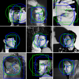
Figure 1: Visualization of the samples from AFLW2000-3D with the worst rotation error. Predictions are blue, ground truth is green. Shown are axes of the local coordinate system, landmarks and bounding box.

Panel 1 visualizes the worst estimates judging by rotation error. It reveals failures in difficult situations with heavy occlusion and a sample with two visible faces. It also shows a few mislabeled samples. In particular in the second row. There the predictions look more plausible than the labels.

Table 2 shows results from various method ablations. Increasing the backbone capacity from MobileNet to ResNet18 improved the metrics insignificantly. Removal of landmark predictions yielded a small improvement in MAE over the BL. Hypothetically, synergetic effects between tasks did not occur in the BL and now more capacity was freed for pose prediction. However the landmark prediction was needed to utilize the annotations of the Face Synthetics data. One might be curious as to the combination of both changes. Indeed, using the ResNet and removing landmark predictions lead to the best geodesic distance error (better than BL + FS) but the MAE metric suffered drastically. The other modifications worsened the accuracy in both metrics. Interestingly, in-plane rotation augmentation had a big impact, where a smaller rotation range yielded intermediate results.

Table 2: Ablation study with different variations of the methodology. Every line means a change from the baseline (OpNet BL). Changes are not cumulative with other lines. ResNet18 means the feature extractor was replaced with it. A minus means removal of the ingredient. "Intensity Aug." refers to the image intensity augmentations, "NLL" to the NLL losses, "Landmarks" to the landmark losses, "In-plane Rot." to the respective rotation augmentation, and "$5^{\circ}$ In-plane Rot." to overridden rotation limits.

. Method Variation MAE Geo. OpNet BL 3.19 5.26 ResNet18 3.18 5.24 - Landmarks 3.16 5.26 ResNet18 - Landmarks 3.27 5.21 - Intensity Aug. 3.24 5.37 - NLL 3.30 5.35 - In-plane Rot. 3.53 5.65 $5^{\circ}$ In-plane Rot. 3.44 5.56

Table 3 shows an ablation study for dataset variations. As can be seen, training on the standard 300W-LP does not yield satisfactory accuracy. The combination of 300W-LP with Face Synthetics is better but also does not yield SOTA accuracy. Improved accuracy was also obtained only with the 300W-LP reproduction. The reason is unknown but it could be explained by a slightly different rotation distribution, the 3D geometry, or the depth estimation. Adding directional lighting and closed eyes improved the accuracy further.

Table 3: Ablation study with different training distributions. "300W-LP" refers to the original dataset, "FS" to Face Synthetics, "R-300W-LP" to the reproduction, "RA-300W-LP" the reproduction with closed eyes and profile illumination, and finally "EX" to the extension generated from LaPa and WFLW.

Notes	Dataset	MAE	Geo.
	300W-LP	3.44	5.44
	300W-LP + FS	3.34	5.36
	R-300W-LP	3.28	5.34
	RA-300W-LP	3.27	5.27
BL	RA-300W-LP + EX	3.19	5.26
BL + FS	RA-300W-LP + EX + FS	3.15	5.23

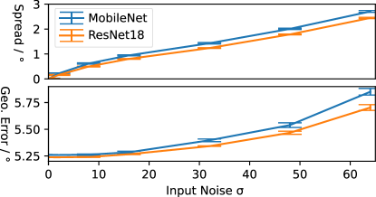
Figure 2: Plots spread and error of rotation predictions due to varying levels of gaussian noise with standard deviation $\sigma$ added to input images. Due to the random nature of the input noise, we can view the networks estimates as random variables underlying a certain probability distribution. "Spread" thus refers to the width of this distribution, measured by the root mean squared geodesic error from the mean. "Geo. Error." refers to the mean of the distribution, approximated by averaging and renormalizing the 4d vector representations of quaternions. This mean is compared to the ground truth. Input and ground truth stem from AFLW2000. Note that the displayed quantities are averages over the dataset and over the evaluation ensemble. The error bars show the standard error of the sample mean w.r.t. the ensemble.

Figure 3: Correlation of the uncertainty estimate with rotation errors. The data points iterate over samples from AFLW2000 and the five BL evaluation networks. Recall that the uncertainty estimate ${\bf\hat{\Sigma}}_{rot}$ is a covariance matrix. Plotted is its Frobenius norm to condense it to a single value.

In spite of the outcome of controlled experiments, in practice I found the ResNet18 variant to produced very noticeably smoother predictions than the BL. This motivated an evaluation on noisy inputs, the result of which is shown in Figure 2. We can recognize that as we add more and more noise, the gap between MobileNet and ResNet variants widens. Moreover, the variance induced by the input noise is generally larger for the MobileNet. The differences are only one or two tenths of degrees at rather high noise levels, so there may be other factors affecting the perceived performance.

Figure 3 demonstrates some degree of effectiveness of the uncertainty estimation, i.e. there is a weak correlation between uncertainty magnitude and prediction error. Note that the failure cases with errors larger than $40^{\circ}$ are correctly attributed with correspondingly large uncertainty.

For the interested reader, the performance on 68-landmark 3D sparse face alignment shall be noted here at last. In the BL + FS experiment the model achieves $3.55\%$ normalized mean 2D error (NME 2D) following the experimental protocol in [4] for the AFLW2000-3D benchmark. The current SOTA, SynergyNet [6], achieves $3.41\%$. The metric measures the error from ground truth landmarks taking only the x and y coordinate into account.

5 Conclusion

The results of this work suggest that the domain gap between popular training data and the real world is significant and limits the effectiveness of current head pose estimation models. Simply combining different flavors of synthetic data, using 300W-LP and Face Synthetics improves generalization dramatically. Moreover, in agreement with [2] it is demonstrated that simple models with relatively simple losses can achieve SOTA performance. However, it is also a limitation of the scope of this work that previous top performing models were not analyzed with the extended training data. It would be of interested for both, HPE as well as face alignment, especially because heavy occlusion, ambiguity and accurate landmark prediction pose a problem to the current model. The uncertainty estimate appears to be effective at detecting failure cases. Both, the MobileNet and the ResNet18-based models are suitable for real-time applications. The MobileNet variant runs very fast on the CPU (Ryzen 9 5900X) even, with ca. 5 ms per inference using only two of its cores. Inference with the ResNet18 variant is slower but its predictions are less sensitive to input noise which may be preferable.

Appendix A Appendix

A.1 Large Pose Expansions

Figure 6: Example frames from the synthetically expanded LaPa dataset.

Figure 7: Example frames from the synthetically expanded LaPa dataset.

References

- [1] Andrea Asperti and Daniele Filippini “Deep Learning for Head Pose Estimation: A Survey” In SN Comput. Sci. 4.4 Berlin, Heidelberg: Springer-Verlag, 2023 DOI: 10.1007/s42979-023-01796-z
- [2] Alejandro Cobo, Roberto Valle, José M. Buenaposada and Luis Baumela “On the representation and methodology for wide and short range head pose estimation” In Pattern Recognition 149, 2024, pp. 110263 DOI: https://doi.org/10.1016/j.patcog.2024.110263
- [3] Heyuan Li et al. “DSFNet: Dual Space Fusion Network for Occlusion-Robust 3D Dense Face Alignment” In Proc. IEEE Conference on Computer Vision and Pattern Recognition, CVPR, 2023, pp. 4531–4540 DOI: 10.1109/CVPR52729.2023.00440
- [4] Xiangyu Zhu et al. “Face Alignment Across Large Poses: A 3D Solution” In Proc. IEEE Conference on Computer Vision and Pattern Recognition, CVPR, 2016, pp. 146–155 DOI: 10.1109/CVPR.2016.23
- [5] Jianzhu Guo et al. “Towards Fast, Accurate and Stable 3D Dense Face Alignment” In Proc. European Conference on Computer Vision, ECCV 12364 Springer, 2020, pp. 152–168 DOI: 10.1007/978-3-030-58529-7\_10
- [6] Cho-Ying Wu, Qiangeng Xu and Ulrich Neumann “Synergy between 3DMM and 3D Landmarks for Accurate 3D Facial Geometry” In International Conference on 3D Vision, 3DV IEEE, 2021, pp. 453–463 DOI: 10.1109/3DV53792.2021.00055
- [7] Jinwei Gu, Xiaodong Yang, Shalini De Mello and Jan Kautz “Dynamic Facial Analysis: From Bayesian Filtering to Recurrent Neural Network” In Proc. IEEE Conference on Computer Vision and Pattern Recognition, CVPR, 2017, pp. 1531–1540 DOI: 10.1109/CVPR.2017.167
- [8] Felix Kuhnke and Jörn Ostermann “Deep Head Pose Estimation Using Synthetic Images and Partial Adversarial Domain Adaption for Continuous Label Spaces” In Proc. International Conference on Computer Vision, ICCV IEEE, 2019, pp. 10163–10172 DOI: 10.1109/ICCV.2019.01026
- [9] Felix Kuhnke and Jörn Ostermann “Domain Adaptation for Head Pose Estimation Using Relative Pose Consistency” In IEEE Trans. Biom. Behav. Identity Sci. 5.3, 2023, pp. 348–359 DOI: 10.1109/TBIOM.2023.3237039
- [10] Erroll Wood et al. “Fake it till you make it: face analysis in the wild using synthetic data alone” In Proc. IEEE Conference on Computer Vision and Pattern Recognition, CVPR, 2021, pp. 3681–3691
- [11] Heng-Wei Hsu et al. “QuatNet: Quaternion-Based Head Pose Estimation With Multiregression Loss” In IEEE Trans. Multim. 21.4, 2019, pp. 1035–1046 DOI: 10.1109/TMM.2018.2866770
- [12] Thorsten Hempel, Ahmed A. Abdelrahman and Ayoub Al-Hamadi “6d Rotation Representation For Unconstrained Head Pose Estimation” In IEEE International Conference on Image Processing, ICIP, Bordeaux, France IEEE, 2022, pp. 2496–2500 DOI: 10.1109/ICIP46576.2022.9897219
- [13] Zeyu Ruan et al. “SADRNet: Self-Aligned Dual Face Regression Networks for Robust 3D Dense Face Alignment and Reconstruction” In IEEE Trans. Image Process. 30, 2021, pp. 5793–5806 DOI: 10.1109/TIP.2021.3087397
- [14] Roberto Valle, José Miguel Buenaposada and Luis Baumela “Multi-Task Head Pose Estimation in-the-Wild” In IEEE Trans. Pattern Anal. Mach. Intell. 43.8, 2021, pp. 2874–2881 DOI: 10.1109/TPAMI.2020.3046323
- [15] Kaiming He, Xiangyu Zhang, Shaoqing Ren and Jian Sun “Deep Residual Learning for Image Recognition” In Proc. IEEE Conference on Computer Vision and Pattern Recognition, CVPR, 2016, pp. 770–778 DOI: 10.1109/CVPR.2016.90
- [16] Mingxing Tan and Quoc V. Le “EfficientNet: Rethinking Model Scaling for Convolutional Neural Networks” In Proc. International Conference on Machine Learning, ICML 97, Proceedings of Machine Learning Research PMLR, 2019, pp. 6105–6114 URL: http://proceedings.mlr.press/v97/tan19a.html
- [17] Ilija Radosavovic et al. “Designing Network Design Spaces” In Proc. IEEE Conference on Computer Vision and Pattern Recognition, CVPR, 2020, pp. 10425–10433 DOI: 10.1109/CVPR42600.2020.01044
- [18] Andrew G. Howard et al. “MobileNets: Efficient Convolutional Neural Networks for Mobile Vision Applications” In CoRR abs/1704.04861, 2017 arXiv: http://arxiv.org/abs/1704.04861
- [19] Mark Sandler et al. “MobileNetV2: Inverted Residuals and Linear Bottlenecks” In Proc. IEEE Conference on Computer Vision and Pattern Recognition, CVPR, 2018, pp. 4510–4520 DOI: 10.1109/CVPR.2018.00474
- [20] Andrew Howard et al. “Searching for MobileNetV3” In Proc. International Conference on Computer Vision, ICCV IEEE, 2019, pp. 1314–1324 DOI: 10.1109/ICCV.2019.00140
- [21] Djork-Arné Clevert, Thomas Unterthiner and Sepp Hochreiter “Fast and Accurate Deep Network Learning by Exponential Linear Units (ELUs)” In Proc. International Conference on Learning Representations, ICLR OpenReview.net, 2016 URL: http://arxiv.org/abs/1511.07289
- [22] Xiangyu Zhu, Xiaoming Liu, Zhen Lei and Stan Z. Li “Face Alignment in Full Pose Range: A 3D Total Solution” In IEEE Trans. Pattern Anal. Mach. Intell. 41.1, 2019, pp. 78–92 DOI: 10.1109/TPAMI.2017.2778152
- [23] Pascal Paysan et al. “A 3D Face Model for Pose and Illumination Invariant Face Recognition” In IEEE International Conference on Advanced Video and Signal Based Surveillance, AVSS IEEE Computer Society, 2009, pp. 296–301 DOI: 10.1109/AVSS.2009.58
- [24] Stephen Milborrow, Tom E. Bishop and Fred Nicolls “Multiview Active Shape Models with SIFT Descriptors for the 300-W Face Landmark Challenge” In International Conference on Computer Vision, ICCV Workshops IEEE, 2013, pp. 378–385 DOI: 10.1109/ICCVW.2013.57
- [25] Christos Sagonas et al. “300 Faces In-The-Wild Challenge: database and results” In Image Vis. Comput. 47, 2016, pp. 3–18 DOI: 10.1016/J.IMAVIS.2016.01.002
- [26] Zhe Chen “Bayesian Filtering: From Kalman Filters to Particle Filters, and Beyond” In Statistics 182, 2003 DOI: 10.1080/02331880309257
- [27] Balaji Lakshminarayanan, Alexander Pritzel and Charles Blundell “Simple and Scalable Predictive Uncertainty Estimation using Deep Ensembles” In Conference on Neural Information Processing Systems, NeurIPS, 2017, pp. 6402–6413 URL: https://proceedings.neurips.cc/paper/2017/hash/9ef2ed4b7fd2c810847ffa5fa85bce38-Abstract.html
- [28] Alex Kendall and Yarin Gal “What Uncertainties Do We Need in Bayesian Deep Learning for Computer Vision?” In Conference on Neural Information Processing Systems, NeurIPS, 2017, pp. 5574–5584 URL: https://proceedings.neurips.cc/paper/2017/hash/2650d6089a6d640c5e85b2b88265dc2b-Abstract.html
- [29] Yingda Yin, Yang Wang, He Wang and Baoquan Chen “A Laplace-inspired Distribution on SO(3) for Probabilistic Rotation Estimation” In Proc. International Conference on Learning Representations, ICLR OpenReview.net, 2023 URL: https://openreview.net/pdf?id=Mvetq8DO05O
- [30] Igor Gilitschenski et al. “Deep Orientation Uncertainty Learning based on a Bingham Loss” In Proc. International Conference on Learning Representations, ICLR OpenReview.net, 2020 URL: https://openreview.net/forum?id=ryloogSKDS
- [31] Nicola De Cao and Wilker Aziz “The Power Spherical distrbution” In Proc. International Conference on Machine Learning, INNF+, 2020
- [32] David Mohlin, Josephine Sullivan and Gérald Bianchi “Probabilistic Orientation Estimation with Matrix Fisher Distributions” In Conference on Neural Information Processing Systems, NeurIPS, 2020 URL: https://proceedings.neurips.cc/paper/2020/hash/33cc2b872dfe481abef0f61af181dfcf-Abstract.html
- [33] C. G. Khatri and K. V. Mardia “The Von Mises-Fisher Matrix Distribution in Orientation Statistics” In Journal of the Royal Statistical Society. Series B (Methodological) 39.1 [Royal Statistical Society, Wiley], 1977, pp. 95–106 URL: http://www.jstor.org/stable/2984884
- [34] Hai Liu et al. “MFDNet: Collaborative Poses Perception and Matrix Fisher Distribution for Head Pose Estimation” In IEEE Trans. Multim. 24, 2022, pp. 2449–2460 DOI: 10.1109/TMM.2021.3081873
- [35] Valentin Peretroukhin et al. “A Smooth Representation of Belief over SO(3) for Deep Rotation Learning with Uncertainty” In Robotics: Science and Systems XVI, Virtual Event / Corvalis, Oregon, USA, 2020 DOI: 10.15607/RSS.2020.XVI.007
- [36] Taeyoung Lee “Bayesian Attitude Estimation With the Matrix Fisher Distribution on SO(3)” In IEEE Trans. Autom. Control. 63.10, 2018, pp. 3377–3392 DOI: 10.1109/TAC.2018.2797162
- [37] Taeyoung Lee “Bayesian Attitude Estimation with Approximate Matrix Fisher Distributions on SO(3)” In IEEE Conference on Decision and Control, CDC IEEE, 2018, pp. 5319–5325 DOI: 10.1109/CDC.2018.8619286
- [38] D.A. Nix and A.S. Weigend “Estimating the mean and variance of the target probability distribution” In Proc. International Conference on Neural Networks (ICNN) 1, 1994, pp. 55–60 vol.1 DOI: 10.1109/ICNN.1994.374138
- [39] Laurens Sluijterman, Eric Cator and Tom Heskes “Optimal training of Mean Variance Estimation neural networks” In Neurocomputing 597, 2024, pp. 127929 DOI: 10.1016/J.NEUCOM.2024.127929
- [40] Du Q. Huynh “Metrics for 3D Rotations: Comparison and Analysis” In J. Math. Imaging Vis. 35.2, 2009, pp. 155–164 DOI: 10.1007/S10851-009-0161-2
- [41] Diederik P. Kingma and Jimmy Ba “Adam: A Method for Stochastic Optimization” In Proc. International Conference on Learning Representations, ICLR OpenReview.net, 2015 URL: http://arxiv.org/abs/1412.6980
- [42] Pavel Izmailov et al. “Averaging Weights Leads to Wider Optima and Better Generalization” In Proc. Conference on Uncertainty in Artificial Intelligence, UAI AUAI Press, 2018, pp. 876–885 URL: http://auai.org/uai2018/proceedings/papers/313.pdf
- [43] Nataniel Ruiz, Eunji Chong and James M. Rehg “Fine-Grained Head Pose Estimation Without Keypoints” In Proc. IEEE Conference on Computer Vision and Pattern Recognition, CVPR Workshops, 2018, pp. 2074–2083 DOI: 10.1109/CVPRW.2018.00281
- [44] René Ranftl et al. “Towards Robust Monocular Depth Estimation: Mixing Datasets for Zero-shot Cross-dataset Transfer” In IEEE Transactions on Pattern Analysis and Machine Intelligence (TPAMI), 2020
- [45] René Ranftl, Alexey Bochkovskiy and Vladlen Koltun “Vision Transformers for Dense Prediction” In Proc. International Conference on Computer Vision, ICCV IEEE, 2021, pp. 12159–12168 DOI: 10.1109/ICCV48922.2021.01196
- [46] Yao Feng, Haiwen Feng, Michael J. Black and Timo Bolkart “Learning an Animatable Detailed 3D Face Model from In-The-Wild Images” In ACM Transactions on Graphics, (Proc. SIGGRAPH) 40.8, 2021 URL: https://doi.org/10.1145/3450626.3459936
- [47] Wojciech Zielonka, Timo Bolkart and Justus Thies “Towards Metrical Reconstruction of Human Faces” In Proc. European Conference on Computer Vision, ECCV Springer, 2022
- [48] Radek Danecek, Michael J. Black and Timo Bolkart “EMOCA: Emotion Driven Monocular Face Capture and Animation” In Proc. IEEE Conference on Computer Vision and Pattern Recognition, CVPR, 2022, pp. 20311–20322
- [49] Tianye Li et al. “Learning a model of facial shape and expression from 4D scans” In ACM Transactions on Graphics, (Proc. SIGGRAPH Asia) 36.6, 2017, pp. 194:1–194:17 URL: https://doi.org/10.1145/3130800.3130813
- [50] Wayne Wu et al. “Look at Boundary: A Boundary-Aware Face Alignment Algorithm” In Proc. IEEE Conference on Computer Vision and Pattern Recognition, CVPR, 2018, pp. 2129–2138 DOI: 10.1109/CVPR.2018.00227
- [51] Yinglu Liu et al. “A New Dataset and Boundary-Attention Semantic Segmentation for Face Parsing” In Proc. AAAI Conference on Artificial Intelligence AAAI Press, 2020, pp. 11637–11644 DOI: 10.1609/AAAI.V34I07.6832
- [52] Ira Kemelmacher-Shlizerman, Steven M. Seitz, Daniel Miller and Evan Brossard “The MegaFace Benchmark: 1 Million Faces for Recognition at Scale” In Proc. IEEE Conference on Computer Vision and Pattern Recognition, CVPR, 2016, pp. 4873–4882 DOI: 10.1109/CVPR.2016.527
- [53] Shuo Yang, Ping Luo, Chen Change Loy and Xiaoou Tang “WIDER FACE: A Face Detection Benchmark” In Proc. IEEE Conference on Computer Vision and Pattern Recognition, CVPR, 2016
- [54] Tsun-Yi Yang, Yi-Ting Chen, Yen-Yu Lin and Yung-Yu Chuang “FSA-Net: Learning Fine-Grained Structure Aggregation for Head Pose Estimation From a Single Image” In Proc. IEEE Conference on Computer Vision and Pattern Recognition, CVPR, 2019, pp. 1087–1096 DOI: 10.1109/CVPR.2019.00118
- [55] Yijun Zhou and James Gregson “WHENet: Real-time Fine-Grained Estimation for Wide Range Head Pose” In British Machine Vision Conference, BMVC, 2020 URL: https://www.bmvc2020-conference.com/assets/papers/0907.pdf
- [56] José Celestino, Manuel Marques, Jacinto C. Nascimento and João Paulo Costeira “2D Image head pose estimation via latent space regression under occlusion settings” In Pattern Recognit. 137, 2023, pp. 109288 DOI: 10.1016/J.PATCOG.2022.109288
- [57] Chien Thai et al. “An Effective Deep Network for Head Pose Estimation without Keypoints” In Proc. International Conference on Pattern Recognition Applications and Methods, ICPRAM SCITEPRESS, 2022, pp. 90–98 DOI: 10.5220/0010870900003122
- [58] Vitor Albiero et al. “img2pose: Face Alignment and Detection via 6DoF, Face Pose Estimation” In Proc. IEEE Conference on Computer Vision and Pattern Recognition, CVPR, 2021, pp. 7617–7627 DOI: 10.1109/CVPR46437.2021.00753
- [59] Redhwan Algabri, Hyunsoo Shin and Sungon Lee “Real-time 6DoF full-range markerless head pose estimation” In Expert Systems with Applications 239, 2024, pp. 122293 DOI: https://doi.org/10.1016/j.eswa.2023.122293
- [60] Tetiana Martyniuk et al. “DAD-3DHeads: A Large-scale Dense, Accurate and Diverse Dataset for 3D Head Alignment from a Single Image” In Proc. IEEE Conference on Computer Vision and Pattern Recognition, CVPR, 2022, pp. 20910–20920 DOI: 10.1109/CVPR52688.2022.02027