Three-dimensional solitons in fractional nonlinear Schrödinger equation with exponential saturating nonlinearity

Abstract

We study the fractional three-dimensional (3D) nonlinear Schrödinger equation with exponential saturating nonlinearity. In the case of the Lévy index $\alpha=1.9$, this equation can be considered as a model equation to describe strong Langmuir plasma turbulence. The modulation instability of a plane wave is studied, the regions of instability depending on the Lévy index, and the corresponding instability growth rates are determined. Numerical solutions in the form of 3D fundamental soliton (ground state) are obtained for different values of the Lévy index. It was shown that in a certain range of soliton parameters it is stable even in the presence of a sufficiently strong initial random disturbance, and the self-cleaning of the soliton from such initial noise was demonstrated.

Key words: Fractional nonlinear Schrödinger equation, three-dimensional soliton, saturating nonlinearity, modulational instability

I Introduction

The concept of a fractional derivative $\partial^{\alpha}/\partial x^{\alpha}$ is a generalization of the ordinary derivative $\partial^{n}/\partial x^{n}$ to the case of a real number $\alpha$, and has a rather long history (more than three hundred years) Oldham1974 ; Samko1993 ; Miller1993 ; Podlubny1999 ; Das2011 that began back in 1695 in the correspondence of Leibnitz with L’Hopital, where the case of $\alpha=1/2$ was considered. Physical applications of the fractional derivative are very diverse and include such areas and phenomena as fractional quantum mechanics, fractional and strange kinetics, fluid mechanics, optics, electromagnetics, diffusion-reaction processes, anomalous transport, fractals, and a number of others Agrawal2004 ; Tarasov2010 ; Herrmann2011 ; Uchaikin2013 ; Malomed2021 ; Malomed2024 ; Mihalache2024 ; Kevrekidis2024 . The concept of fractional quantum mechanics, which stimulated many works on physical applications of the fractional derivative, was formulated by Laskin in Laskin2000 ; Laskin2002 ; Laskin2018 , and the fractional quantum mechanical Schrödinger equation was introduced by generalizing the Feynman path integral over Lévy trajectories corresponding random Lévy flights in the theory of Brownian motion. In this case, the number $\alpha$ (Lévy index) characterizing the fractionality of the Laplacian in the Schrödinger equation takes values in the range $0<\alpha\leq 2$.

The fractional Laplacian (with the Riesz fractional derivative) is defined as

$$(-\Delta)^{\alpha/2}f(\mathbf{x})=\mathcal{F}^{-1}(|\mathbf{k}|^{\alpha}\mathcal{F}f)$$

$$=\frac{1}{(2\pi)^{D}}\int|\mathbf{k}|^{\alpha}\hat{f}(\mathbf{k})\mathrm{e}^{i\mathbf{k}\cdot\mathbf{x}}d^{D}\mathbf{k},$$ (1)

where $\hat{f}=\mathcal{F}f$ is the Fourier transform of $f$, and $D$ is the spatial dimension ($D=1,2,3$). Another definition of the fractional Laplacian (with the Caputo fractional derivative) often used in applications is

$$(-\Delta)^{\alpha/2}f(\mathbf{x})=\frac{2^{\alpha-1}\alpha\Gamma((D+\alpha)/2)}{\sqrt{\pi^{D}}\Gamma(1-\alpha/2)}$$

$$\times\,\mathrm{P}.\,\mathrm{V}.\int\frac{f(\mathbf{x})-f(\mathbf{x}^{\prime})}{|\mathbf{x}-\mathbf{x}^{\prime}|^{D+\alpha}}d^{D}\mathbf{x}^{\prime},\quad\mathrm{for}\quad 0<\alpha\leq 2,$$ (2)

where P. V. stands for the Cauchy principal value. Both of these definitions are equivalent in Schwartz space Samko1993 ; Kwasnicki2017 . Note that there is also a fairly large number of other definitions of the fractional derivative, both classical and new ones introduced quite recently Oliveira2014 . In this paper, for the fractional Laplacian we use Eq. (1).

One of the most physically significant models with fractional derivatives is the fractional nonlinear Schrödinger equation (NLS). It generalizes the well-known NLS equation to the case of a fractional Laplacian. Physical applications of the fractional NLS equation in most cases concern nonlinear optics (see, e.g., reviews Malomed2021 ; Malomed2024 and references therein). The fractional Davey-Stewartson equations (one of the generalizations of the two-dimensional NLS equation) with the Lévy index $\alpha=3/4$ was obtained in Davey2015 for nonlinear surface water waves.

Numerical solutions of the one-dimensional (1D) fractional NLS equation with cubic nonlinearity in the form of a fundamental soliton (ground state) for different Lévy indices $0<\alpha<2$ were found in Klein2014 . There, the evolution of an initial profile different from the soliton one was also studied, and both focusing and defocusing nonlinearity were considered. In the focusing case, at $\alpha=1$ there is a collapse in the so-called critical regime (negative Hamiltonian and the 1D norm exceeds the soliton 1D norm), and for $0<\alpha<1$ in the supercritical regime (a sufficiently large 1D norm). The 1D fractional NLS equation with cubic nonlinearity was also studied in detail in Chen2018 . In particular, analytical soliton solutions were obtained using a variational approach for different values of $\alpha$. It is shown that solitons are stable for $1<\alpha<2$, but for $\alpha=1$ the soliton collapses. Various problems within the framework of the fractional NLS equation (modulation instability, the presence of a trapping potential, two-dimensional structures, including vortex solitons, etc.) were considered in Malomed2021 ; Malomed2024 ; Zhang2017 ; Malomed2020 ; Ovolabi2016 . The possible applicability of the inverse scattering transfrom method for the 1D fractional NLS equation was discussed in Ablowitz2022 .

In connection with the problem of Langmuir plasma turbulence Zakharov1972 ; Thornhill1978 ; Goldman1984 , in Adjemyan1989 the three-dimensional (3D) stochastic NLS equation with external noise was studied using quantum field theory approach. In particular, using the quantum field renormalization group method, it was shown that in this case the usual linear dispersion in the NLS equation $\omega=k^{2}$ (assuming $\psi\sim\exp(i\mathbf{k}\cdot\mathbf{x}-i\omega t)$) is replaced by $\omega=k^{2-\gamma_{a}}$, where $\gamma_{a}$ is the so-called anomalous dimension known from quantum field theory, and $\gamma_{a}=0.0804$. The effective NLS equation with such a corrected dispersion no longer contains a stochastic term. This equation appears to be the only example of a fractional three-dimensional NLS equation that has physical applications. As is known, an arbitrary initial perturbation with a negative Hamiltonian or formal stationary solutions of the conventional three-dimensional NLS equation with cubic nonlinearity collapse (blow-up), that is, become singular in a finite time Sulem1999 . The same is true (as shown by the 1D examples given above) for the fractional three-dimensional NLS equation with $\alpha<2$. In reality, the formation of a singularity is prevented by dissipation or higher-order nonlinearities. For nonlinear Langmuir waves, the collapse can be arrested for the exponential saturable nonlinearity corresponding to the Boltzmann distribution of plasma particles Laedke1984 ; Lashkin2020 .

In this paper, we study the three-dimensional fractional NLS equation with exponential saturating nonlinearity and numerically obtain soliton solutions (ground states) for different values of the Lévy index. We pay special attention to the case of the Levy index $\alpha=2-\gamma_{a}\sim 1.9$ corresponding to an important physical application in the problem of Langmuir plasma turbulence. By direct numerical simulation, we show the stability of solitons in a certain range of parameters satisfying the Vakhitov-Kolokolov criterion. For the first time, the phenomenon of self-cleaning of a stable soliton from a sufficiently strong initial random disturbance is demonstrated for the fractional NLS equation.

The paper is organized as follows. The basic model equation is presented in Sec. II. In Sec. III, we consider modulation instability of a plane wave and find the corresponding instability thresholds and instability growth rates. Sec. IV, soliton solutions are found, and a numerical analysis of the stability of solitons is performed. Finally, Sec. V concludes the paper.

II Model equation

We consider the fractional nonlinear Schrödinger equation with exponential saturable nonlinearity in spatial dimension $D=3$,

$$i\frac{\partial\psi}{\partial t}-(-\Delta)^{\alpha/2}\psi+\left[1-\exp(-|\psi|^{2})\right]\psi=0.$$ (3)

As noted in the Introduction, the fractional Laplacian with $\alpha=2-\gamma_{a}\sim 1.9$ in Eq. (3) corresponds to the corrected linear dispersion law (in fact, a renormalized propagator) of Langmuir waves for the stochastic NLS equation with cubic nonlinearity in the theory of Langmuir plasma wave turbulence. On the other hand, the exponential nonlinearity in the three-dimensional NLS equation with the usual Laplacian ($\alpha=2$) prevents the phenomenon of wave collapse and can results in the existence of stable nonlinear coherent structures such as solitons and vortex solitons (they can be treated as ”elementary bricks” of strong Langmuir turbulence). In particular, Eq. (3) with $\alpha=1.9$ can be considered as a model equation for Langmuir turbulence without the phenomenon of catastrophic collapse.

Equation (3) conserves the 3D norm

$$N=\int|\psi|^{2}d^{3}\mathbf{x},$$ (4)

and Hamiltonian

$$H=\!\!\int\!\left\{\mathrm{Re}\!\left[\psi^{\ast}(-\Delta)^{\alpha/2}\psi\right]-|\psi|^{2}-\exp(-|\psi|^{2})+1\right\}d^{3}\mathbf{x},$$ (5)

and can be written in the hamiltonian form

$$i\frac{\partial\psi}{\partial t}=\frac{\delta H}{\delta\psi^{\ast}}.$$ (6)

The evolution of an arbitrary initial disturbance within the framework of Eq. (3) occurs under the influence of two competing factors - dispersion and nonlinearity. Dispersion causes the wave packet to spread and, in this sense, counteracts collapse. However, as $\alpha$ decreases, the dispersion becomes increasingly unable to arrest the collapse (blow-up). For example, at $\alpha=1$, even one-dimensional solitons of the fractional NLS equation with cubic nonlinearity are unstable and collapse. At sufficiently large amplitudes $|\psi|\gg 1$, the nonlinear term in Eq. (3) effectively becomes linear. This is an example of the so-called saturable nonlinearity (not necessarily exponential), which is often encountered, for example, in nonlinear optics Kivshar_book2003 . Saturable nonlinearities cause collapse arrest (or beam self-focusing in two-dimensional models) and can lead to the existence of stable coherent structures.

III Modulational instability

Equation (3) has an exact solution in the form of a monochromatic plane wave

$$\psi=|\psi_{0}|\exp(i\mathbf{k}_{0}\cdot\mathbf{x}-i\omega_{0}t)$$ (7)

with a frequency depending on the amplitude $\psi_{0}$,

$$\omega_{0}=k_{0}^{\alpha}+\exp(-|\psi_{0}|^{2})-1.$$ (8)

Consider the stability of such a plane wave. The perturbed plane wave solution has the form

$$\psi=(|\psi_{0}|+\delta\psi)\exp(i\mathbf{k}_{0}\cdot\mathbf{x}-i\omega_{0}t),$$ (9)

where

$$\delta\psi=\psi^{+}\mathrm{e}^{i\mathbf{k}\cdot\mathbf{x}-i\Omega t}+\psi^{-}\mathrm{e}^{-i\mathbf{k}\cdot\mathbf{x}+i\Omega t},$$ (10)

is a linear modulation with the frequency $\Omega$ and the wave vector $\mathbf{k}$. Linearizing Eq. (3) in $\delta\psi$, we get the nonlinear dispersion relation

$$1-\left[1-\exp(-|\psi_{0}|^{2})\right]\left[\frac{1}{\omega_{\mathbf{k}_{0}+\mathbf{k}}-\omega_{\mathbf{k}_{0}}-\Omega}\right.$$

$$\left.+\frac{1}{\omega_{\mathbf{k}_{0}-\mathbf{k}}-\omega_{\mathbf{k}_{0}}+\Omega}\right]=0,$$ (11)

where $\omega_{\mathbf{q}}=|\mathbf{q}|^{\alpha}$ is the linear dispersion relation for Eq. (3). In the case of short-wave modulations $\mathbf{k}\gg\mathbf{k}_{0}$, and taking into account that $\omega_{\mathbf{k}}$ is even function, Eq. (11) becomes

$$\Omega^{2}=\omega_{\mathbf{k}}\left\{\omega_{\mathbf{k}}-2[1-\exp(-|\psi_{0}|^{2})]\right\}.$$ (12)

Equation (12) predicts a purely growing instability (modulational instability) provided

$$2[1-\exp(-|\psi_{0}|^{2})]>k^{\alpha},$$ (13)

that is, when the amplitude threshold is exceeded,

$$|\psi_{0}|>\sqrt{-\ln(1-k^{\alpha}/2)}.$$ (14)

The instability growth rate $\gamma$ is given by

$$\gamma=\sqrt{2k^{\alpha}[1-\exp(-|\psi_{0}|^{2})]-k^{2\alpha}}.$$ (15)

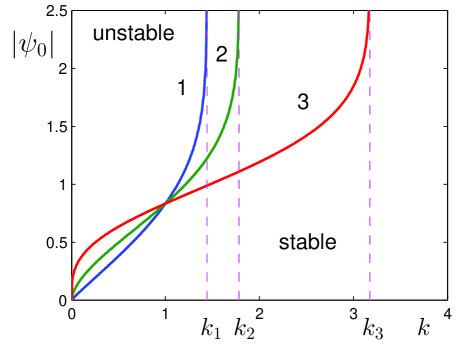
Figure 1: Modulational instability region on the plane $(|\psi_{0}|,k)$. The areas above the corresponding curves correspond to instability. The numbers above the curves correspond to different $\alpha$: 1 - $\alpha=1.9$, 2 - $\alpha=1.2$, and 3 - $\alpha=0.6$. The corresponding critical wave numbers $k_{1}=1.44$, $k_{2}=1.78$, and $k_{3}=3.17$ are indicated.

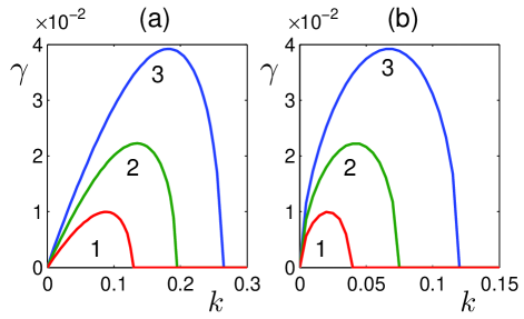
Figure 2: Dependence of the instability growth rate $\gamma$ on wave number $k$ for different amplitude values $\psi_{0}$; (a) $\alpha=1.9$; (b) $\alpha=1.2$. The numbers under the curves correspond to different amplitudes: 1 - $|\psi_{0}|=0.1$, 2 - $|\psi_{0}|=0.15$, and 3 - $|\psi_{0}|=0.2$.

For each fixed value of $\alpha$, instability occurs only for wave numbers $k$ exceeding the critical value $k_{\mathrm{cr}}=2^{1/\alpha}$, and at $k\rightarrow k_{\mathrm{cr}}$ the instability threshold tends to infinity. The region of instability determined by Eq. (14) on the plane $(k,|\psi_{0}|)$ is shown in Fig. 1 for different values of $\alpha$, namely $\alpha=1.9$, $\alpha=1.2$ and $\alpha=0.6$. The corresponding values of the critical wave number $k_{\mathrm{cr}}$ are equal to $k_{1}=1.44$, $k_{2}=1.78$ and $k_{3}=3.17$, respectively. The optimal wave number of perturbations, that is, corresponding to the maximum instability growth rate in Eq. (15) is $k_{\mathrm{opt}}=[1-\exp(-|\psi_{0}|^{2})]^{1/\alpha}$, and the corresponding instability growth rate is

$$\gamma_{m}=1-\exp(-2|\psi_{0}|^{2}),$$ (16)

and does not depend on $\alpha$. Dependence of the instability growth rate $\gamma$ on wave number $k$ for different amplitude values $\psi_{0}$ in the cases $\alpha=1.9$ and $\alpha=1.2$ is shown in Fig. 2.

In the opposite case of short-wave modulations with $\mathbf{k}\ll\mathbf{k}_{0}$, using

$$\omega_{\mathbf{k}_{0}\pm\mathbf{k}}\sim\omega_{\mathbf{k}_{0}}\pm\frac{\partial\omega_{\mathbf{k}_{0}}}{\partial\mathbf{k}_{0}}\cdot\mathbf{k}+\frac{1}{2}\frac{\partial^{2}\omega_{\mathbf{k}_{0}}}{\partial\mathbf{k}_{0}^{2}}k^{2},$$ (17)

from Eq. (11) we obtain

$$(\Omega-\mathbf{k}\cdot\mathbf{v}_{g})^{2}=\frac{1}{4}(\omega_{\mathbf{k}_{0}}^{\prime\prime})^{2}k^{4}-\omega_{\mathbf{k}_{0}}^{\prime\prime}k^{2}[1-\exp(-|\psi_{0}|^{2})],$$ (18)

where

$$\mathbf{v}_{g}=\frac{\partial\omega_{\mathbf{k}_{0}}}{\partial\mathbf{k}_{0}}=\frac{\partial(\mathbf{k}_{0}\cdot\mathbf{k}_{0})^{\alpha/2}}{\partial\mathbf{k}_{0}}=\alpha k_{0}^{\alpha-2}\mathbf{k}_{0}$$ (19)

is the group velocity, and $\omega_{\mathbf{k}_{0}}^{\prime\prime}=\alpha(\alpha-1)k_{0}^{\alpha-2}$. If the amplitude threshold $|\psi_{0}|$ determined by

$$4[1-\exp(-|\psi_{0}|^{2})]>\omega_{\mathbf{k}_{0}}^{\prime\prime}k^{2},$$ (20)

is exceeded, then Eq. (18) corresponds to convective instability when growing disturbances are carried away with the group velocity $\mathbf{v}_{g}$, and the instability growth rate is given by

$$\gamma=2k\sqrt{\omega_{\mathbf{k}_{0}}^{\prime\prime}[1-\exp(-|\psi_{0}|^{2})-\omega_{\mathbf{k}_{0}}^{\prime\prime}k^{2}/4]}.$$ (21)

IV Three-dimensional soliton

We look for stationary solutions of Eq. (3) of the form

$$\psi(\mathbf{r},t)=u(\mathbf{r})\exp(i\lambda t),$$ (22)

where $\lambda>0$ is a free parameter, and the function $u(\mathbf{r})$ is assumed to be real without loss of generality. Then from Eq. (3) we have

$$-\lambda u-(-\Delta)^{\alpha/2}u+\left[1-\exp(-u^{2})\right]u=0.$$ (23)

An analytical solution of Eq. (23) is impossible, but in addition, due to the exponential form of nonlinearity and the impossibility of analytical calculation of the corresponding integrals, the variational approach used for the fractional NLS equation with cubic nonlinearity Malomed2021 ; Chen2018 ; Qiu2020 , is also apparently inapplicable. Note that the solutions of the fractional NLS equation ($\alpha\neq 2$) with general nonlinearities decay algebraically at infinity as $\sim 1/|\mathbf{x}|^{D+\alpha}$ Frank2013 ; Frank2016 ; Li2024 , in contrast to the case $\alpha=2$, where the solutions are localized exponentially.

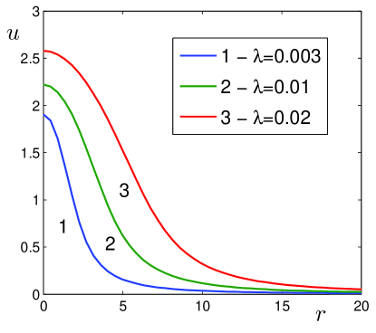
Figure 3: Radial profiles of a spherically symmetric soliton (ground state) for the case of the Lévi index $\alpha=1.2$ for different values of $\lambda$.

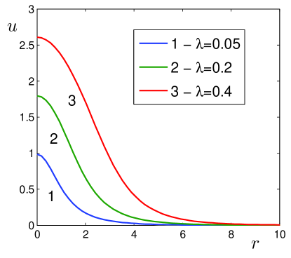
Figure 4: Radial profiles of a spherically symmetric soliton (ground state) for the case of the Lévi index $\alpha=1.9$ for different values of $\lambda$.

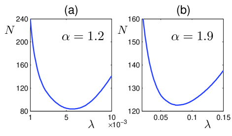
Figure 5: The 3D norm $N$ of the fundamental soliton as a function of the parameter $\lambda$: (a) Lévy index $\alpha=1.2$; (b) Lévy index $\alpha=1.9$.

We numerically find localized solutions of Eq. (23) using the Petviashvili method Petviashvili1976 ; Petviashvili_book1992 ; Lakoba2007 . Periodic boundary conditions are assumed and, due to the algebraic behavior at infinity, the box length is taken to be sufficiently large that the solution at the boundary is negligible small. The advantage of the Petviashvili method is that it is used in Fourier space (that is, the fractional Laplacian is introduced in a simple natural way) and, in combination with the Fast Fourier Transform (FFT), does not require much computational time even on very high resolution grids. Note that there is a modification of this method Lashkin2008_77 ; Lashkin2008_78 that uses only physical space and is therefore applicable to equations containing an explicit dependence on spatial variables, but in this case the method is slower (FFT is not used). After the Fourier transform, defined here for an arbitrary function $f(\mathbf{r})$ as

$$f_{\mathbf{k}}=\int f(\mathbf{r})\exp(-i\mathbf{k}\cdot\mathbf{r})d^{3}\mathbf{r},$$ (24)

equation (23) is written in the form

$$G_{\mathbf{k}}^{-1}u_{\mathbf{k}}=N_{\mathbf{k}},$$ (25)

where $G_{\mathbf{k}}=-1/(\lambda+k^{\alpha})$ and $N_{\mathbf{k}}$ accounts for the nonlinear term. Then the Petviashvili iteration procedure at the $n$-th iteration is

$$u_{\mathbf{k}}^{(n+1)}=sG_{\mathbf{k}}N_{\mathbf{k}}^{(n)},$$ (26)

where $s$ is the so-called stabilizing factor determined by

$$s=\left(\frac{\int|u_{\mathbf{k}}^{(n)}|^{2}d^{3}\mathbf{k}}{\int u_{\mathbf{k}}^{\ast,(n)}G_{\mathbf{k}}N_{\mathbf{k}}^{(n)}d^{3}\mathbf{k}}\right)^{\gamma},$$ (27)

and the parenthetic superscript denotes the iteration step index. The nonlinear term at each step was first calculated in physical space and then its Fourier transform $N_{\mathbf{k}}$ was used. For power-law nonlinearity $u^{p}$, the fastest convergence occurs for

$$\gamma=\frac{p}{p-1}.$$ (28)

Petviashvili formulated this in the form of a mnemonic rule, but the choice of the optimal value of $\gamma$ was rigorously justified in Ref. Pelinovsky2004 . The procedure always converges to the nonlinear ground state, i. e. fundamental soliton, regardless of the initial guess. Moreover, the rate of convergence is almost independent of the initial approximation. For nonlinearity other than power-law, the value of $\gamma$ corresponding to the fastest convergence is chosen empirically and $1<\gamma<p/(p-1)$, where $p$ is the smallest exponent in the Taylor series expansion of nonlinearity. For the exponential nonlinearity in Eq. (23), we chose $\gamma=1.3$. We used $u(\mathbf{r})=\lambda^{1/2}\exp(-\lambda^{1/2}r^{2})$ as the initial guess in all runs. The iterations rapidly converge to a three-dimensional spherically symmetric soliton solution. The progressive iterations were terminated when the value $|s-1|$ fell below $10^{-15}$. Radial profiles of the three-dimensional soliton solutions for Lévy index $\alpha=1.2$ and for Lévy index $\alpha=1.9$ at different values of $\lambda$ are shown in Fig. 3 and Fig. 4, respectively.

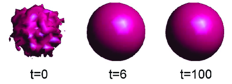
Figure 6: Self-cleaning and stable dynamics of the fundamental soliton for the Lévy index $\alpha=1.9$ and $\lambda=0.15$. The initial state is perturbed by the white noise with the parameter $\varepsilon=0.05$; the shape (isosurface $|\psi|=1.35$) of the perturbed soliton at the initial moment $t=0$, at $t=6$, and at $t=100$.

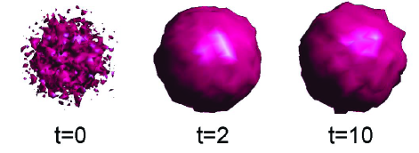
Figure 7: Evolution of the fundamental soliton for the Lévy index $\alpha=1.9$ and $\lambda=0.15$ with a sufficiently strong random initial perturbation ($\varepsilon=0.3$); the shape (isosurface $|\psi|=1.35$) of the perturbed soliton at the initial moment $t=0$, at $t=2$, and at $t=10$.

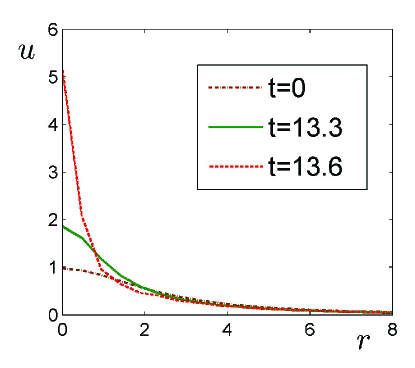
Figure 8: Unstable dynamics of the soliton for the Lévy index $\alpha=1.9$ and $\lambda=0.03$; radial profiles at the initial moment $t=0$, at $t=13.3$, and at $t=13.6$.

The dependences of the 3D norm $N$ of the fundamental soliton on the parameter $\lambda$ are shown in Fig. 5 for the cases of the Lévy index $\alpha=1.2$ and $\alpha=1.9$. It can be seen that these dependencies are nonmonotonic functions $N(\lambda)$ of the parameter $\lambda$. The minimum points are $\lambda_{\mathrm{cr},1}=0.057$ and $\lambda_{\mathrm{cr},2}=0.076$ for the cases $\alpha=1.2$ and $\alpha=1.9$, respectively. The corresponding 3D norms are $N_{\mathrm{min},1}=84$ and $N_{\mathrm{min},2}=123$. For the case of the Lévy index $\alpha=2$ (ordinary Laplacian), the critical value $\lambda=0.101$ was found in Laedke1984 . For an ordinary NLS equation ($\alpha=2$) in an arbitrary spatial dimension $D$ and with a rather arbitrary form of nonlinearity, the Vakhitov-Kolokolov criterion is valid. It was first formulated in Vakhitov1973 and later rigorously justified and generalized in Rypdal1986 ; Berge1998 (see also references therein). According to this criterion, a sufficient (but not necessary) condition for the stability of the ground state is

$$\frac{\partial N}{\partial\lambda}>0.$$ (29)

As far as we know, the applicability of the Vakhitov-Kolokolov criterion for a fractional NLS equation has not yet been studied. Nevertheless, from Fig. 5 it is clear that for the Lévy index $\alpha=1.2$ in the region $\lambda>\lambda_{\mathrm{cr},1}$, as well as for the Lévy index $\alpha=1.9$ in the region $\lambda>\lambda_{\mathrm{cr},2}$, the corresponding ground states satisfy the Vakhitov-Kolokolov criterion (29), and therefore one may expect that they are stable.

To verify the results predicted by the Vakhitov-Kolokolov criterion, we solved numerically the dynamical equation (3) initialized with our computed solutions of the form of fundamental soliton with added Gaussian noise. The initial condition was taken in the form $\psi(\mathbf{x},0)=\psi_{0}(\mathbf{r})[1+\varepsilon f(\mathbf{r})]$, where $\psi_{0}(\mathbf{r})$ is the numerically calculated solution, $f(\mathbf{r})$ is the white Gaussian noise with variance $\sigma^{2}=1$, and the parameter of perturbation $\varepsilon=0.05-0.3$. The time integration was performed by the Runge-Kutta-Merson method with the variable time step and local error control (we used the corresponding NAG (Numerical Algorithms Group) routine NAG ). The linear term (fractional Laplacian) was calculated in spectral space and then transformed into physical space. The 3D norm conserved with a relative accuracy $<10^{-5}$ during the simulations. In the case of the Lévy index $\alpha=1.9$, the evolution of soliton with $\lambda=0.15$, i. e. satisfying the stability condition $\lambda>\lambda_{\mathrm{cr},2}$, with an initial rather strong random perturbation with $\varepsilon=0.05$ is presented in Fig. 6. It can be seen that the soliton turns out to be robust and stable. During the evolution, the soliton undergoes self-cleaning from the initial random disturbance. At time $t=6$, the soliton completely restores its unperturbed shape, and then evolves without distortion ($t=100$). Simulations with other values of $\lambda$ in the stability region, as well as for the Lévy index $\alpha=1.2$, also result in self-cleaning of the soliton. If the intensity of the initial random disturbance is sufficiently large, the soliton self-cleanses itself from noise, simultaneously deforming, but does not undergo any significant shape distortions. An example of such an evolution of a soliton subjected at the initial moment of time to a strong random perturbation with $\varepsilon=0.3$ is shown in Fig. 7. Self-cleaning of stable localized structures in the form of multidimensional solitons and vortex solitons from initial noise within the framework of conventional NLS equation ($\alpha=2$) with different types of nonlinearity was observed numerically in a number of works Malomed2005 ; Malomed2006 ; Malomed2007PLA ; Lashkin2020 ; Lashkin2008_78 . Note that in our case, self-cleaning of the soliton from the initial noise occurs for a 3D soliton with algebraically decaying tails caused by the fractional Laplacian in the model under consideration. The time evolution of the soliton with the Lévy index $\alpha=1.9$ and $\lambda=0.03$, that is, corresponding to an unstable region $\lambda<\lambda_{\mathrm{cr},2}$ in accordance with the formal Vakhitov-Kolokolov criterion (29), is shown in Fig. 8. During the evolution, the 3D norm $N$ has been conserved with an accuracy $<10^{-7}$. Until time $t\lesssim 13$ the soliton shape remains unchanged. This time is equal in order of magnitude to the inverse modulation instability growth rate $\sim 1/\lambda$ ($\lambda$ corresponds to the square of amplitude of the plane wave) of the fastest growing mode in Eq. (16). At subsequent moments in time $t=13.3$ and $t=13.6$, the amplitude of the soliton rapidly increases, and at the same time soliton contracts in accordance with the preservation of the 3D norm. That is, the instability becomes explosive in a nonlinear regime, resulting in a singularity in a finite time (blow-up). Thus, as predicted by the criterion (29), in the unstable region the 3D soliton collapses.

V Conclusion

We have studied the fractional 3D nonlinear Schrödinger equation with exponential saturating nonlinearity. We have pointed out that in the special case of the Lévy index $\alpha=1.9$, this equation describes the dynamics of strong Langmuir turbulence of plasma waves. The modulation instability of a plane wave has been studied and a nonlinear dispersion equation has been derived. In particular cases of perturbations corresponding to small and large wavelengths compared to the length of plane wave, the modes of convective and absolute instability have been predicted, respectively. The regions of instability depending on the Lévy index, and the corresponding modulational instability growth rates have been obtained.

Numerical solutions in the form of 3D fundamental soliton (ground state) have been obtained for different values of the Lévy index. The obtained dependences of the 3D norm of the soliton on the free parameter $\lambda$ (for plasma turbulence it corresponds to a nonlinear frequency shift) turn out to be non-monotonic and correspond to two regions for which the Vakhitov-Kolokolov stability criterion is formally valid. Numerical simulation has shown that in a certain range of soliton parameters it is stable even in the presence of a sufficiently strong initial random disturbance, and self-cleaning of the soliton from such initial noise has been demonstrated.

In connection with the soliton self-cleaning effect, we would like to make a short comment. As is known, a one-dimensional NLS equation with $\alpha=2$ and cubic nonlinearity is completely integrable. In particular, any localized initial condition (including a random perturbation) with a sufficiently large 1D norm in the course of evolution results in the emergence of a pure soliton (or several solitons) while the non-soliton part is dispersed and carried to infinity. Therefore, in this context, the self-cleaning of a soliton in the presence of a random disturbance is a rigorously established fact. Multidimensional generalizations of the NLS equation are not completely integrable, and even in cases where the type of nonlinearity allows the existence of stable multidimensional solitons, direct analogy is not applicable here. Nevertheless, in our case, considering a random disturbance against the background of a pure soliton as a localized but dispersive wave packet, one can treat the self-cleaning as the spreading and disappearance at infinity of the non-soliton dispersive part in the course of evolution.

For the model under consideration, the question of the value of the Lévy index $\alpha$ at which 3D solitons become unstable remains open (recall that 1D solitons of the fractional NLS equation with cubic nonlinearity collapse if $\alpha<1$). In the case under consideration with saturating exponential nonlinearity (as apparently for other saturating nonlinearities) these values of the critical index depend on the parameter $\lambda$ in contrast to the conventional model with non-saturating nonlinearity. This problem is expected to be studied in the future.

Declaration of competing interest

The authors declare that they have no known competing financial interests or personal relationships that could have appeared to influence the work reported in this paper.

All authors have no conflicts of interest associated with this publication, and there has been no financial support for this work that could have influenced its outcome.

CRediT authorship contribution statement

V. M. Lashkin: Conceptualization, Methodology, Validation, Formal analysis, Investigation. O. K. Cheremnykh: Conceptualization, Methodology, Validation, Formal analysis, Investigation.

Data availability

No data was used for the research described in the article.

References

References

- (1) K. Oldham, J. Spanier, The fractional calculus (Academic Press, New York, 1974).
- (2) S. G. Samko, A. A. Kilbas, and O. I. Marichev, Fractional integrals and derivatives (Gordon and Breach, Yverdon, 1993).
- (3) K. S. Miller, B. Ross, An Introduction to the Fractional Calculus and Fractional Differential Equations (Wiley, New York, 1993).
- (4) I. Podlubny, Fractional Differential Equations (Academic Press, San Diego, 1999).
- (5) S. Das, Functional Fractional Calculus, 2nd edition (Springer-Verlag, Berlin, 2011).
- (6) O. P. Agrawal, J. A. Tenreiro-Machado, and I. Sabatier, Fractional Derivatives and Their Applications: Nonlinear Dynamics (Springer-Verlag, Berlin, 2004).
- (7) V. E. Tarasov, Fractional Dynamics: Applications of Fractional Calculus to Dynamics of Particles, Fields and Media (Springer, New York, 2010).
- (8) R. Herrmann, Fractional calculus: an introduction for physicists (World Scientific, Singapore, 2011).
- (9) V. V. Uchaikin, Fractional derivatives for physicists and engineers (Springer, Berlin, 2013).
- (10) B. A. Malomed, Optical solitons and vortices in fractional media: a mini-review of recent results, Photonics 8, 353 (2021).
- (11) B. A. Malomed, Basic fractional nonlinear-wave models and solitons, Chaos 34, 022102 (2024).
- (12) D. Mihalache, Localized structures in optical media and Bose-Einstein condensates: An overview of recent theoretical and experimental results, Rom. Rep. Phys. 76, 402 (2024).
- (13) Fractional Dispersive Models and Applications: Recent Developments and Future Perspectives, edited by P. G. Kevrekidis and Jesús Cuevas-Maraver (Springer, Berlin, 2024).
- (14) N. Laskin, Fractional quantum mechanics, Phys. Rev. E 62, 3135 (2000).
- (15) N. Laskin, Fractional Schrödinger equation, Phys. Rev. E 66, 056108 (2002).
- (16) N. Laskin, Fractional Quantum Mechanics (World Scientific Publishing, Singapore, 2018).
- (17) M. Kwaśnicki, Ten equivalent definitions of the fractional Laplace operator. Fract. Calc. Appl. Anal., 20, 7-51 (2017).
- (18) E. C. de Oliveira and J. A. Tenreiro-Machado, A review of definitions for fractional derivatives and integral, Mathematical Problems in Engineering 2014, 238459 (2014).
- (19) C. Obrecht, J.-C. Saut, Remarks on the full dispersion Davey-Stewartson equation systems, Communications on pure and applied analysis 14, 1547-1561 (2015).
- (20) C. Klein, C. Sparber, and P. Markowich, Numerical study of fractional nonlinear Schrödinger equations, Proc. R. Soc. A 470, 20140364 (2014).
- (21) M. Chen, S. Zeng, D. Lu, W. Hu, and Q. Guo, Optical solitons, self-focusing, and wave collapse in a space-fractional Schrödinger equation with a Kerr-type nonlinearity, Phys. Rev. E 98, 022211 (2018).
- (22) L. Zhang, Z. He, C. Conti, Z. Wang, Y. Hu, D. Lei, Y. Li, D. Fan, Modulational instability in fractional nonlinear Schrödinger equation, Commun. Nonlinear Sci. Numer. Simulat. 48, 531-540 (2017).
- (23) Y. Qiu, B. A. Malomed, D. Mihalache, X. Zhu, X. Peng, Y. He, Stabilization of single- and multi-peak solitons in the fractional nonlinear Schrödinger equation with a trapping potential, Chaos, Solitons & Fractals 140, 110222 (2020).
- (24) K. M. Owolabi and A. Atangana, Numerical solution of fractional-in-space nonlinear Schrödinger equation with the Riesz fractional derivative, Eur. Phys. J. Plus 131, 335 (2016).
- (25) M. J. Ablowitz, J. B. Been, and L. D. Carr, Fractional integrable nonlinear soliton equations, Phys. Rev. Lett. 128, 184101 (2022).
- (26) V. E. Zakharov, Collapse of Langmuir waves, Sov. Phys. JETP 35, 908-914 (1972).
- (27) S. G. Thornhill, D. ter Haar, Langmuir turbulence and modulational instability, Phys. Rep. 43, 43-99 (1978).
- (28) M. V. Goldman, Strong turbulence of plasma waves, Rev. Mod. Phys. 56, 709-735 (1984).
- (29) L. Ts. Adzhemyan, A. N. Vasil’ev, M. Gnatich, and Yu. M. Pis’mak, Quantum field renormalization group in the theory of stochastic Langmuir turbulence, Theor. Math. Phys. 78, 260-272 (1989).
- (30) C. Sulem, P.-L. Sulem, The nonlinear Schrödinger equation: self-focusing and wave collapse (Springer-Verlag, New York, 1999).
- (31) E. W. Laedke and K. H. Spatschek, Stable three-dimensional envelope solitons, Phys. Rev. Lett. 52, 279 (1984).
- (32) V. M. Lashkin, Stable three-dimensional Langmuir vortex soliton, Phys. Plasmas 27, 042106 (2020).
- (33) Y. S. Kivshar and G. P. Agrawal, Optical Solitons: From Fibers to Photonic Crystals (Academic Press, San Diego, 2003).
- (34) Y. Qiu, B. A. Malomed, D. Mihalache, X. Zhu, L. Zhang, Y. He, Soliton dynamics in a fractional complex Ginzburg-Landau model, Chaos Solitons Fractals 131, 109471 (2020).
- (35) R. L. Frank, E. Lenzmann, Uniqueness of nonlinear ground states for fractional Laplacians in , Acta Math. 210, 261-318 (2013).
- (36) R. L. Frank, E. Lenzmann, and L. Silvestre, Uniqueness of radial solutions for the fractional Laplacian, Comm. Pure Appl. Math. 69, 1671-1726 (2016).
- (37) X. Lia and L. Song, Uniqueness of positive solutions for fractional Schrödinger equations with general nonlinearities, arXiv:2401.02795 [math.AP].
- (38) V. I. Petviashvili, Equation of an extraordinary soliton, Sov. J. Plasma Phys. 2, 257-258 (1976).
- (39) O. A. Pokhotelov and V. I. Petviashvili, Solitary Waves in Plasmas and in the Atmosphere (Gordon and Breach, Reading, 1992).
- (40) T. I. Lakoba, J. Yang, A generalized Petviashvili iteration method for scalar and vector Hamiltonian equations with arbitrary form of nonlinearity, J. Comput. Phys. 226, 1668-1692 (2007).
- (41) V. M. Lashkin, Two-dimensional multisolitons and azimuthons in Bose-Einstein condensates, Phys. Rev. A 77, 025602 (2008).
- (42) V. M. Lashkin, Stable three-dimensional spatially modulated vortex solitons in Bose-Einstein condensates, Phys. Rev. A 78, 033603 (2008).
- (43) D. E. Pelinovsky, Yu. A. Stepanyants, Convergence of Petviashvili’s iteration method for numerical approximation of stationary solutions of nonlinear wave equations, SIAM J. Numer. Anal. 42 1110-1127 (2004).
- (44) M. G. Vakhitov and A. A. Kolokolov, Stationary solutions of the wave equation in the medium with nonlinearity saturation, Radiophys. Quantum Electron. 16, 783 (1973).
- (45) J. J. Rasmussen and K. Rypdal, Blow-up in nonlinear Schroedinger equations-I: A general review, Physica Scripta 33, 481-497 (1986).
- (46) L. Bergé, Wave collapse in physics: principles and applications to light and plasma waves, Phys. Rep. 303, 259-370 (1998).
- (47) NAG Fortran Library, Mark 18 (Numerical Algorithms Group, Oxford, 1999).
- (48) B. A. Malomed, D. Mihalache, F. Wise, and L. Torner, Spatiotemporal optical solitons, J. Opt. B: Quantum Semiclass. Opt. 7, R53-R72 (2005).
- (49) D. Mihalache, D. Mazilu, F. Lederer, Y. V. Kartashov, L.-C. Crasovan, L. Torner, and B. A. Malomed, Stable vortex tori in the three-dimensional cubic-quintic Ginzburg-Landau equation, Phys. Rev. Lett. 97, 073904 (2006).
- (50) B. A. Malomed, F. Lederer, D. Mazilu, D. Mihalache, On stability of vortices in three-dimensional self-attractive Bose-Einstein condensates, Phys. Lett. A 361, 336-340 (2007).