Fast Proxy Experiment Design for Causal Effect Identification
Abstract
Identifying causal effects is a key problem of interest across many disciplines. The two long-standing approaches to estimate causal effects are observational and experimental (randomized) studies. Observational studies can suffer from unmeasured confounding, which may render the causal effects unidentifiable. On the other hand, direct experiments on the target variable may be too costly or even infeasible to conduct. A middle ground between these two approaches is to estimate the causal effect of interest through proxy experiments, which are conducted on variables with a lower cost to intervene on compared to the main target. Akbari et al. [2022] studied this setting and demonstrated that the problem of designing the optimal (minimum-cost) experiment for causal effect identification is NP-complete and provided a naive algorithm that may require solving exponentially many NP-hard problems as a sub-routine in the worst case. In this work, we provide a few reformulations of the problem that allow for designing significantly more efficient algorithms to solve it as witnessed by our extensive simulations. Additionally, we study the closely-related problem of designing experiments that enable us to identify a given effect through valid adjustments sets.
1 Introduction
Identifying causal effects is a central problem of interest across many fields, ranging from epidemiology all the way to economics and social sciences. Conducting randomized (controlled) trials provides a framework to analyze and estimate the causal effects of interest, but such experiments are not always feasible. Even when they are, gathering sufficient data to draw statistically significant conclusions is often challenging because of the limited number of experiments often (but not solely) due to the high costs.
Observational data, which is usually more abundant and accessible, offers an alternative avenue. However, observational studies bring upon a new challenge: the causal effect may not be identifiable due to unmeasured confounding, making it impossible to draw inferences based on the observed data [Pearl, 2009, Hernán and Robins, 2006].
A middle ground between the two extremes of observational and experimental approaches was introduced by Akbari et al. [2022], where the authors suggested conducting proxy experiments to identify a causal effect that is not identifiable based on solely observational data. To illustrate the need for proxy experiments, consider the following drug-drug interaction example, based on the example in Lee et al. [2020a].
Example 1.
(Complex Drug Interactions and Cardiovascular Risk) Consider a simplified example of the interaction between antihypertensives (), anti-diabetics (), renal function modulators (), and their effects on blood pressure () and cardiovascular disease (). Blood pressure and cardiovascular health are closely linked. can influence the need for , and directly affects . reduces cardiovascular risk () by controlling blood sugar. directly impacts . Unmeasured factors confound these relationships: shared health conditions can influence the prescribing of both and ; lifestyle factors influence both and ; and common conditions like metabolic syndrome can affect both and . Fig. 2(a) illustrates the causal graph, where directed edges represent direct causal effects, and bidirected edges indicate unmeasured confounders. Suppose we are interested in estimating the intervention effect of and on , which is not identifiable from observational data; Moreover, we cannot directly intervene on these variables because and are essential for managing immediate, life-threatening conditions. Instead, we can intervene on , which is a feasible and safer approach due to the broader range of treatment options and more manageable risks associated with adjusting anti-diabetic medications. As we shall see, intervention on suffices for identifying the effect of and on .
Selecting the optimal set of proxy experiments is not straightforward in general. In particular, Akbari et al. [2022] proved that the problem of finding the minimum-cost intervention set to identify a given causal effect, hereon called the MCID problem, is NP-complete and provided a naive algorithm that requires solving exponentially many instances of the minimum hitting set problem in the worst case. As the minimum hitting set problem is NP-complete itself, this results in a doubly exponential runtime for the algorithm proposed by Akbari et al. [2022], which is computationally intractable even for graphs with a modest number of vertices. Moreover, Akbari et al. [2022]’s algorithm was tailored to a specific class of causal effects in which the effect of interest is a functional of an interventional distribution where the intervention is made on every variable except one district of the causal graph111See Section 2 the definition of a district.. For a general causal effect, their algorithm’s complexity includes an additional (super-)exponential multiplicative factor, where the exponent is the number of districts.
In this work, we revisit the MCID problem and develop tractable algorithms by reformulating the problem as instances of well-known problems, such as the weighted maximum satisfiability and integer linear programming problems. Furthermore, we analyze the problem of designing minimum cost interventions to obtain a valid adjustment set for a query. This problem not only merits attention in its own right, but also serves as a proxy for MCID. Our contributions are as follows:
-
•
We formulate the MCID problem in terms of a partially weighted maximum satisfiability, integer linear programming, submodular function maximization, and reinforcement learning problem. These reformulations allow us to propose new, and in practice, much faster algorithms for solving the problem optimally.
-
•
We formulate and study the problem of designing minimum-cost experiments for identifying a given effect through finding a valid adjustments set. Besides the practical advantages of valid adjustment, including ease of interpretability and tractable sample complexity, this approach enables us to design a polynomial-time heuristic algorithm for the MCID problem that outperforms the heuristic algorithms provided by Akbari et al. [2022].
-
•
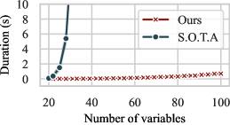
We present new numerical experiments that demonstrate the exceptional speed of our exact algorithms when compared to the current state-of-the-art, along with our heuristic algorithm showcasing superior performance over previous heuristic approaches.
2 Problem formulation
We begin by reviewing relevant graphical definitions. An acyclic directed mixed graph (ADMG) is a graph with directed () and bidirected () edges such that the directed edges form no cycles [Richardson, 2003]. We denote an ADMG by a tuple , where , , and represent the set of vertices, directed edges, and bidirected edges, respectively. Note that is a set of ordered pairs of vertices in , whereas is a set of unordered pairs of vertices.
Vertices of represent variables of the system under consideration, while the edges represent causal relations between them. We use the terms ‘variable’ and ‘vertex’ interchangeably. When , we say is a parent of and is a child of . The set of parents of denoted by . We denote by , the induced subgraph of over vertices . A subset of is said to form a district in if any pair of vertices are connected through a bidirected path in . In other words, is a connected component through its bidirected edges. We say is an ancestor of if there is a directed path for some . We denote the set of ancestors of in the subgraph by . Note that . When , we drop the subscript for ease of notation.
Let be two disjoint sets of variables. The probability distribution of under a (possibly hypothetical) intervention on setting its value to is often represented as either , using Rubin’s potential outcomes model [Rubin, 1974], or using Pearl’s operator [Pearl, 2009]. We will adopt the shorthand to denote this interventional distribution222This interventional distribution is often mistakenly referred to as the causal effect of on . However, a causal effect, such as an average treatment effect or a quantile treatment effect, is usually a specific functional of this probability distribution for different values of ..
Definition 1 (Identifiability).
An interventional distribution is identifiable given an ADMG and the intervention set family , with , over the variables corresponding to , if is uniquely computable as a functional of the members of .
Remark 1.
We will now define the important notion of a hedge, which, as we will see shortly after, is central to deciding the identifiability of an interventional distribution given the data at hand.
Definition 2 (Hedge).
Let be a district in . We say forms a hedge for if (i) is a district in , and (ii) every vertex is an ancestor of in (i.e., ). We denote by the set of hedges formed for in .
For example, in Fig. 2(b), has two hedges given by .
Remark 2.
Definition 2 is different from the original definition of Shpitser and Pearl [2006]. The original definition was found to not correspond one-to-one with non-identifiability, as pointed out by Shpitser [2023]. However, our modified definition above is a sound and complete characterization of non-identifiability, as it coincides with the criterion put forward by Huang and Valtorta [2006] as well as the ‘reachable closure’ of Shpitser [2023].
Definition 3 (Hedge hull Akbari et al., 2022).
Let be a district in ADMG . Also let be the set of all hedges formed for in . The union of all hedges in , denoted by is said to be the hedge hull of in .
For instance, in Fig. 2(d), the hedge hull of is and the hedge hull of is When a set consists of more than one district, we simply define the hedge hull of as the union of the hedge hulls of each district of . The hedge hull of a set can be found through a series of at most depth-first-searches. For the sake of completeness, we have included the algorithm for finding a hedge hull in Appendix B.1.
The following proposition from Lee et al. [2020a] and Kivva et al. [2022] establishes the graphical criterion for deciding the identifiability of a causal effect given a set family of interventions.
Proposition 1.
Let be an ADMG over the vertices . Also let be disjoint sets of variables. Define , and let be the (unique) set of maximal districts in . The interventional distribution is identifiable given and the intervention set family , if and only if for every , there exists an intervention set such that (i) , and (ii) there is no hedge formed for in .
Note that there is no hedge formed for in if and only if hits every hedge of (i.e., for any hedge , ). For ease of presentation, we will use to denote that and hits every hedge formed for . For example, given the graph in Fig. 2(d) and with an intervention set family that hits every hedge is
Minimum-cost intervention for causal effect identification (MCID) problem. Let be a known function333Although it only makes sense to assign non-negative costs to interventions, adopting non-negative costs is without loss of generality. If certain intervention costs are negative, one can shift all the costs equally so that the most negative cost becomes zero. This constant shift would not affect the minimization problem in any way. indicating the cost of intervening on each vertex . An infinite cost is assigned to variables where an intervention is not feasible. Given and disjoint sets , our objective is to find a set family with minimum cost such that is identifiable given ; that is, for every district of , there exists such that . Since every is a subset of , the space of such set families is the power set of the power set of .
To formalize the MCID problem, we first write the cost of a set family as where with a slight abuse of notation, we denoted the cost of by . The MCID problem then can be formalized as follows.
| (1) |
where is the set of maximal districts of , and represents the power set of the power set of . In the special case where comprises a single district, the MCID problem can be presented in a simpler way.
Proposition 2 (Akbari et al., 2022).
If comprises a single maximal district , then the optimization in (1) is equivalent to the following optimization:
| (2) |
That is, the problem reduces to finding the minimum-cost set that ‘hits’ every hedge formed for .
Recall example Example 1, we were interested in finding the least costly proxy experiment to identify the effect of and on . By Proposition 2, this problem is equivalent to finding an intervention set with the least cost (i.e., a set of proxy experiments) that hits every hedge of in the transformed graph (Fig. 2(b)). If , then the optimal solution would be .
In the remainder of the paper, we consider the problem of identification of for a given pair , and with defined as , unless otherwise stated. We will first consider the case where comprises a single district, and then generalize our findings to multiple districts.
3 Reformulations of the min-cost intervention problem
In the previous section, we delineated the MCID problem as a discrete optimization problem. This problem, cast as Eq. 1, necessitates search within a doubly exponential space, which is computationally intractable. Algorithm 2 of [Akbari et al., 2022] is an algorithm that conducts this search and eventually finds the optimal solution. However, even when comprises a single district, this algorithm requires, in the worst case, exponentially many calls to a subroutine which solves the NP-complete minimum hitting set problem on exponentially many input sets, hence resulting in a doubly exponential complexity. More specifically, their algorithm attempts to find a set of minimal hedges, where minimal indicates a hedge that contains no other hedges, and solves the minimum hitting set problem on them. However, there can be exponentially many minimal hedges, as shown for example in Fig. 2(c). Letting , then any set that contains one vertex from each level (i.e., directed distance from ) is a minimal hedge, of which there are
Furthermore, the computational complexity of Algorithm 2 of Akbari et al. [2022] grows super-exponentially in the number of districts of . This is due to the necessity of exhaustively enumerating every possible partitioning of these districts and executing their algorithm once for each partitioning.
In this section, we reformulate the MCID problem as a weighted partially maximum satisfiability (WPMAX-SAT) problem [Fu and Malik, 2006], and an integer linear programming (ILP) problem. In Appendix D, we also present reformulations as a submodular maximization problem and a reinforcement learning problem. The advantage of these new formulations is two-fold: (i) compared to Algorithm 2 of [Akbari et al., 2022], we state the problem as a single instance of another problem for which a range of well-studied solvers exist, and (ii) these formulations allow us to propose algorithms with computational complexity that is quadratic in the number of districts of . We will see how these advantages translate to drastic performance gains in Section 5.
3.1 Min-cost intervention as a WPMAX-SAT problem
We begin with constructing a 3-SAT formula that is satisfiable if and only if the given query is identifiable. To this end, we define variables for each vertex , where is the cardinality of the hedge hull of , excluding . Intuitively, is going to indicate whether or not vertex is reachable from after iterations of alternating depth-first-searches on directed and bidirected edges. This is in line with the workings of Algorithm 2 for finding the hedge hull of . In particular, if a vertex is reachable after iterations, that is, , then is a member of the hedge hull of . The query of interest is identifiable if and only if , that is, the hedge hull of contains no other vertices. Therefore, we ensure that the formula is satisfiable if and only if for every . The formal procedure for constructing this formula is as follows.
SAT Construction Procedure.
Suppose a causal ADMG and a set are given, where is a district in . Suppose is the hedge hull of in , where without loss of generality, , and . We will construct a corresponding boolean expression in conjunctive normal form (CNF) using variables for and . For ease of presentation, we also define for all , . The construction is carried out in steps, where in each step, we conjoin new clauses to the previous formula using ‘and’. The procedure is as follows:
-
•
For odd , for each directed edge , add to .
-
•
For even , for each bidirected edge , add both clauses and to .
-
•
Finally, at step , add clauses to the expression for every .
Theorem 1.
The 3-SAT formula constructed by the procedure above given and has a satisfying solution where for and for if and only if intersects every hedge formed for in ; i.e., is a feasible solution to the optimization in Eq. 2.
The proofs of all our results appear in Appendix C. The first corollary of Theorem 1 is that the SAT formula is always satisfiable, for instance by setting for every . The second (and more important) corollary is that the optimal solution to Eq. 2 corresponds to the satisfying assignment for the SAT formula that minimizes
| (3) |
This suggests that the problem in Eq. 2 can be reformulated as a weighted partial MAX-SAT (WPMAX-SAT) problem. WPMAX-SAT is a generalization of the MAX-SAT problem, where the clauses are partitioned into hard and soft clauses, and each soft clause is assigned a weight. The goal is to maximize the aggregate weight of the satisfied soft clauses while satisfying all of the hard ones.
To construct the WPMAX-SAT instance, we simply define all clauses in as hard constraints, and add a soft clause with weight for every . The former ensures that the assignment corresponds to a feasible solution of Eq. 2, while the latter ensures that the objective in Eq. 3 is minimized – which, consequently, minimizes the cost of the corresponding intervention.
Multiple districts.
The formulation above was presented for the case where is a single district. In the more general case where has multiple maximal districts, we can extend our formulation to solve the general problem of Eq. 1 instead. To this end, we will use the following lemma.
Lemma 1.
Let be the set of maximal districts of , where . There exists an intervention set family of size that is optimal for identifying .
Based on Lemma 1, we can assume w.l.o.g. that the optimizer of Eq. 1 contains exactly intervention sets . We will modify the SAT construction procedure described in the previous section to allow for multiple districts as follows. For any district , we will construct copies of the SAT expression, one corresponding to each intervention set , . Each copy is built on new sets of variables indexed by , except the variables with index , which are common across districts. We introduce variables , which will serve as indicators for whether hits all the hedges formed for . We relax every clause corresponding to the -th copy by conjoining a literal with an ‘or.’ Intuitively, this is because it suffices to hit the hedges formed for with some . Additionally, we add the clauses for any to ensure that for every district, there is at least one intervention set that hits every hedge. This modified procedure, detailed in Algorithm 3, appears in Section B.2. The following result generalizes Theorem 1.
Theorem 2.
Suppose , a set of its vertices with maximal districts , and an intervention set family are given. Define , i.e., the cardinality of the hedge hull of excluding itself. The SAT formula constructed by Algorithm 3 has a satisfying solution where for every , there exists such that (i) , (ii) for every , and (iii) for every , if and only if is a feasible solution to optimization of Eq. 1.
Constructing the corresponding WPMAX-SAT instance follows the same steps as the case for a single district, except that the soft clauses are of the form with weight for every and .
Remark 3.
The SAT construction of Algorithm 3 is advantageous because its complexity grows quadratically with the number of districts of in the worst case. In contrast, the runtime of algorithm proposed by Akbari et al. [2022], when consists of multiple districts, is super-exponential in the number of districts, because they need to execute their single-district algorithm at least as many times as the number of partitions of the set .
Min-cost intervention as an ILP problem.
The WPMAX-SAT formulation of Section 3.1 paves the way for a straightforward formulation of an integer linear program (ILP) for the MCID problem. ILP allows for straightforward integration of various constraints and objectives, enabling flexible modeling of potential extra constraints. Moreover, there exist efficient and scalable solvers for ILP [Gearhart et al., 2013, Gurobi Optimization, LLC, 2023]. To construct the ILP instance for the MCID problem, it suffices to represent every clause in the boolean expression of Algorithm 3 as a linear inequality. For example, clauses of the form is rewritten as . The soft constraints may be rewritten as a sum to maximize over, given by Eq. 3.
4 Minimum-cost intervention design for adjustment criterion
A special case of identifying interventional distributions is identification through adjusting for confounders. A set is a valid adjustment set for if is identified as
| (4) |
where the expectation w.r.t. . Adjustment sets have received extensive attention in the literature because of the straightforward form of the identification formula (Eq. 4) and the intuitive interpretation: is the set of confounders that we need to adjust for to identify the effect of interest. The simple form of Eq. (4) has the added desirable property that its sample efficiency and asymptotic behavior are easy to analyze [Witte et al., 2020, Rotnitzky and Smucler, 2020, Henckel et al., 2022]. A complete graphical criterion for adjustment sets was given by Shpitser et al. [2010]. As an example, when all parents of (i.e., ) are observable, they form a valid adjustment set. However, in the presence of unmeasured confounding, no valid adjustment sets may exist. Below, we generalize the notion of adjustment sets to the interventional setting.
Definition 4 (Generalized adjustment).
We say is a generalized adjustment set for under intervention if is identified as where represents the distribution after intervening on and the expectation is w.r.t. .
Note that unlike the classic adjustment, the generalized adjustment is always feasible – a trivial generalized adjustment can be formed by choosing and .
Equipped with Definition 4, we can define a problem closely linked to Eq. 2, but with a (possibly) narrower set of solutions, which can be defined as follows: find the minimum-cost intervention such that a generalized adjustment exists for under :
| (5) |
Observation. The existence of a valid (generalized) adjustment set ensures the identifiability of . As such, any feasible solution to the optimization above is also a feasible solution to Eq. 2. Eq. 5 is not only a problem that deserves attention in its own right, but also serves as a proxy for our initial problem (Eq. 2).
To proceed, we need the following definitions. Given an ADMG , let be the ADMG resulting from replacing every bidirected edge by a vertex and two directed edges . In particular, , and . Note that is a directed acyclic graph (DAG). The moralized graph of , denoted by , is the undirected graph constructed by moralizing as follows: The set of vertices of is . Each pair of vertices are connected by an (undirected) edge if either (i) , or (ii) such that .
Throughout this section, we assume without loss of generality that is minimal in the following sense: there exists no proper subset such that everywhere444This is to say, the third rule of do calculus does not apply to . More precisely, there is no such that is d-separated from given in .. Otherwise, we apply the third rule of do calculus [Pearl, 2009] as many times as possible to make minimal. We also assume w.l.o.g. that as other vertices are irrelevant for our purposes [Lee et al., 2020b]. We will utilize the following graphical criterion for generalized adjustment.
Lemma 2.
Let be two disjoint sets of vertices in such that is minimal as defined above. Set is a generalized adjustment set for under intervention if (i) , and (ii) is a vertex cut555This corresponds to blocking all the backdoor paths between and , in the modified graph . between and in , where , and is the ADMG resulting from omitting all edges incoming to and all edges outgoing of .
Based on the graphical criterion of Lemma 2, we present the following polynomial-time666The computational bottleneck of the algorithm is an instance of minimum vertex cut problem, which can be solved using any off-the-shelf max-flow algorithm. algorithm for finding an intervention set that allows for identification of the query of interest in the form of a (generalized) adjustment. This algorithm will find the intervention set and the corresponding generalized adjustment set simultaneously. We begin by making minimal in the sense of applicability of rule 3 of do calculus. Then we omit all edges going out of , and construct the graph as defined above – by replacing bidirected edges with vertices representing unobserved confounding. Finally, we construct an (undirected) vertex cut network as follows. Each vertex is represented by two connected vertices in . If , then has a cost of zero, and has cost . Otherwise, both and have infinite costs. Intuitively, choosing will correspond to including in the adjustment set, whereas choosing in the cut would imply intervention on . We connect to all vertices corresponding to with index , i.e., . This serves two purposes: (i) if is included in the cut (corresponding to an intervention on ), all connections between and its parents are broken, and (ii) when is not included in the cut (corresponding to no intervention on ), connects the parents of to each other, completing the necessary moralization process. We solve for the minimum vertex cut between vertices with index corresponding to and . Algorithm 1 summarizes this approach. In the solution set , the vertices with index represent the vertices where an intervention is required, while those with index represent the generalized adjustment set under this intervention.
Theorem 3.
Let be the output returned by Algorithm 1 for the query .
Then,
- is a generalized adjustment set for under intervention .
- is the minimum-cost intervention for which there exists a generalized adjustment set based on the graphical criterion of Lemma 2.
Remark 4.
Algorithm 1 enforces identification based on (generalized) adjustment for . As discussed above, this algorithm can be utilized as a heuristic approach to solve the MCID problem in (2). In this case, one can run the algorithm on the hedge hull of rather than the whole graph. We prove in Appendix C that the cost of this approach is always at most as high as heuristic algorithm 1 proposed by Akbari et al. [2022], and is often in practice lower, as verified by our experiments.
5 Experiments
In this section, we present numerical experiments that showcase the empirical performance and time efficiency of our proposed exact and heuristic algorithms. A comprehensive set of numerical experiments analyzing the impact of various problem parameters on the performance of these algorithms, along with the complete implementation details, is provided in Appendix A. We first compare the time efficiency of our exact algorithms: WPMAX-SAT and ILP, with the exact algorithm of Akbari et al. [2022]. Then, we present results pertaining to performance of our heuristic algorithm. All experiments, coded in Python, were conducted on a machine equipped two Intel Xeon E5-2680 v3 CPUs, 256GB of RAM, and running Ubuntu 20.04.3 LTS.
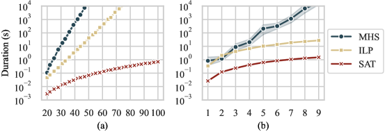
Results on exact algorithms. We compare the performance of the WPMAX-SAT formulation, the ILP formulation, and Algorithm 2 of Akbari et al. [2022], called Minimal Hedge Solver (MHS) from hereon. We used the RC2 algorithm [Ignatiev et al., 2019], and the Gurobi solver [Gurobi Optimization, LLC, 2023], to solve the WPMAX-SAT problem, and the ILP, respectively. We ran each algorithm for solving the MCID problem on randomly generated Erdos-Renyi [Erdos and Renyi, 1960] ADMG graphs with directed and bidirected edge probabilities ranging from to , in increments of . We performed two sets of simulations: for single-district and multiple-district settings, respectively. In the single-district case, we varied , the number of vertices, from to , while in the multiple-district case, we fixed and varied the number of districts from to .
We plot the average time taken to solve each graph versus the number of vertices (single-district) in Fig. 3(a) and versus the number of districts () in Fig. 3(b). The error bands in our figures represent 99% confidence intervals. Focusing on the single-district plot, we observe that both of our algorithms are faster than MHS of Akbari et al. [2022] for all graph sizes. More specifically, ILP is on average one to two orders of magnitude faster than MHS, while WPMAX-SAT is on average four to five orders of magnitude faster. All three algorithms exhibit exponential growth in time complexity with the number of vertices, which is expected as the problem is NP-hard, but WPMAX-SAT grows at a much slower rate than the other two algorithms. This is likely due to RC2’s ability of exploiting the structure of the WPMAX-SAT problem to reduce the search space efficiently. In the multiple-district case, we observe that the time complexity of both WPMAX-SAT and ILP grows polynomially with the number of districts, while the time complexity of MHS grows exponentially. This is consistent with theory, as MHS iterates over all partitions of the set of districts, which grows exponentially with the number of districts.
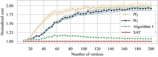
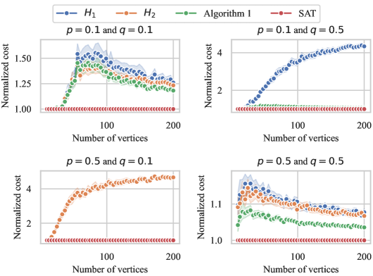
Results on inexact algorithms. We compared Algorithm 1, our proposed heuristic, with the two best performing heuristic algorithms in Akbari et al. [2022], and . We ran each algorithm on randomly generated Erdos-Renyi ADMG graphs with directed and bidirected edge probabilities in , with ranging from to . We randomly sampled the cost of each vertex from a discrete uniform distribution on . In Fig. 4, we plot the normalized cost of each algorithm, computed by dividing the cost of the algorithm by the cost of the optimal solution, provided by WPMAX-SAT. Observe that Algorithm 1 consistently outperforms and for all graph sizes.
6 Conclusion
We presented novel formulations and efficient algorithms for the MCID problem, offering substantial improvements over existing methods. Our work on designing minimum-cost experiments for obtaining valid adjustment sets demonstrates both practical and theoretical advancements. We highlighted the superior performance of our proposed methods through extensive numerical experiments. We envision designing efficient approximation algorithms for MCID as future work.
References
- Akbari et al. [2022] Sina Akbari, Jalal Etesami, and Negar Kiyavash. Minimum cost intervention design for causal effect identification. In Proceedings of the 39th International Conference on Machine Learning, volume 162 of Proceedings of Machine Learning Research, pages 258–289. PMLR, 17–23 Jul 2022. URL https://proceedings.mlr.press/v162/akbari22a.html.
- Pearl [2009] Judea Pearl. Causality. Cambridge university press, 2009.
- Hernán and Robins [2006] Miguel A Hernán and James M Robins. Estimating causal effects from epidemiological data. Journal of Epidemiology & Community Health, 60(7):578–586, 2006.
- Lee et al. [2020a] Sanghack Lee, Juan D Correa, and Elias Bareinboim. General identifiability with arbitrary surrogate experiments. In Uncertainty in artificial intelligence, pages 389–398. PMLR, 2020a.
- Richardson [2003] Thomas Richardson. Markov properties for acyclic directed mixed graphs. Scandinavian Journal of Statistics, 30(1):145–157, 2003.
- Rubin [1974] Donald B Rubin. Estimating causal effects of treatments in randomized and nonrandomized studies. Journal of educational Psychology, 66(5):688, 1974.
- Kivva et al. [2022] Yaroslav Kivva, Ehsan Mokhtarian, Jalal Etesami, and Negar Kiyavash. Revisiting the general identifiability problem. In Uncertainty in Artificial Intelligence, pages 1022–1030. PMLR, 2022.
- Shpitser and Pearl [2006] Ilya Shpitser and Judea Pearl. Identification of joint interventional distributions in recursive semi-markovian causal models. In AAAI, pages 1219–1226, 2006.
- Shpitser [2023] Ilya Shpitser. When does the id algorithm fail? arXiv preprint arXiv:2307.03750, 2023.
- Huang and Valtorta [2006] Yimin Huang and Marco Valtorta. Pearl’s calculus of intervention is complete. In Proceedings of the 22nd Conference on Uncertainty in Artificial Intelligence, 2006, pages 13–16, 2006.
- Fu and Malik [2006] Zhaohui Fu and Sharad Malik. On solving the partial max-sat problem. In Armin Biere and Carla P. Gomes, editors, Theory and Applications of Satisfiability Testing - SAT 2006, page 252–265, Berlin, Heidelberg, 2006. Springer. ISBN 978-3-540-37207-3. doi: 10.1007/11814948_25.
- Gearhart et al. [2013] Jared Lee Gearhart, Kristin Lynn Adair, Justin David Durfee, Katherine A Jones, Nathaniel Martin, and Richard Joseph Detry. Comparison of open-source linear programming solvers. Technical report, Sandia National Lab.(SNL-NM), Albuquerque, NM (United States), 2013.
- Gurobi Optimization, LLC [2023] Gurobi Optimization, LLC. Gurobi Optimizer Reference Manual, 2023. URL https://www.gurobi.com.
- Witte et al. [2020] Janine Witte, Leonard Henckel, Marloes H Maathuis, and Vanessa Didelez. On efficient adjustment in causal graphs. Journal of Machine Learning Research, 21(246):1–45, 2020.
- Rotnitzky and Smucler [2020] Andrea Rotnitzky and Ezequiel Smucler. Efficient adjustment sets for population average causal treatment effect estimation in graphical models. Journal of Machine Learning Research, 21(188):1–86, 2020.
- Henckel et al. [2022] Leonard Henckel, Emilija Perković, and Marloes H Maathuis. Graphical criteria for efficient total effect estimation via adjustment in causal linear models. Journal of the Royal Statistical Society Series B: Statistical Methodology, 84(2):579–599, 2022.
- Shpitser et al. [2010] Ilya Shpitser, Tyler VanderWeele, and James M Robins. On the validity of covariate adjustment for estimating causal effects. In Proceedings of the 26th Conference on Uncertainty in Artificial Intelligence, UAI 2010, pages 527–536. AUAI Press, 2010.
- Lee et al. [2020b] Sanghack Lee, Juan D. Correa, and Elias Bareinboim. General identifiability with arbitrary surrogate experiments. In Proceedings of The 35th Uncertainty in Artificial Intelligence Conference, page 389–398. PMLR, August 2020b. URL https://proceedings.mlr.press/v115/lee20b.html.
- Ignatiev et al. [2019] Alexey Ignatiev, Antonio Morgado, and Joao Marques-Silva. Rc2: an efficient maxsat solver. Journal on Satisfiability, Boolean Modeling and Computation, 11(1):53–64, September 2019. ISSN 15740617. doi: 10.3233/SAT190116.
- Erdos and Renyi [1960] Paul Erdos and Alfred Renyi. On the evolution of random graphs. Publ. Math. Inst. Hungary. Acad. Sci., 5:17–61, 1960.
- Morgado et al. [2014] Antonio Morgado, Carmine Dodaro, and Joao Marques-Silva. Core-guided maxsat with soft cardinality constraints. In Barry O’Sullivan, editor, Principles and Practice of Constraint Programming, page 564–573, Cham, 2014. Springer International Publishing. ISBN 978-3-319-10428-7. doi: 10.1007/978-3-319-10428-7_41.
- IBM Corporation [2023] IBM Corporation. IBM ILOG CPLEX Optimization Studio CPLEX User’s Manual, 2023. URL https://www.ibm.com/analytics/cplex-optimizer.
- Forrest and Lougee-Heimer [2023] J.J.H. Forrest and R. Lougee-Heimer. CBC User Guide. COIN-OR, 2023. URL https://github.com/coin-or/Cbc.
- Lauritzen et al. [1990] Steffen L Lauritzen, A Philip Dawid, Birgitte N Larsen, and H-G Leimer. Independence properties of directed markov fields. Networks, 20(5):491–505, 1990.
- Nemhauser et al. [1978] G. L. Nemhauser, L. A. Wolsey, and M. L. Fisher. An analysis of approximations for maximizing submodular set functions—i. Mathematical Programming, 14(1):265–294, December 1978. ISSN 1436-4646. doi: 10.1007/BF01588971.
Appendix
Appendix A Implementation details and further experimental results
A.1 Implementation details
Our codebase is implemented fully in Python. We use the PySAT library for formulating and solving the WPMAX-SAT problem, and the PuLP library for formulating and solving the ILP problem.
Solving the WPMAX-SAT problem.
There are several algorithms to solve the WPMAX-SAT instance to optimality. These algorithms include RC2 [Ignatiev et al., 2019] and OLL [Morgado et al., 2014], both of which are core-based algorithms that utilize unsatisfiable cores to iteratively refine the solution. In this context, a “core” refers to an unsatisfiable subset of clauses within the CNF formula that cannot be satisfied simultaneously under any assignment. These algorithms relax the unsatisfiable soft clauses in the core by adding relaxation variables and enforce cardinality constraints on these variables. By strategically increasing the bounds on these cardinality constraints or modifying the weights of soft clauses based on the cores identified, the algorithms efficiently reduce the search space and converge on the maximum weighted set of satisfiable clauses, thereby solving the WPMAX-SAT problem optimally.
Solving the ILP problem.
Similarly, with the ILP formulation of the MCID problem presented in Section 3, we can utilize exact algorithms designed for solving ILP problems to find an optimal solution. ILP solvers work by formulating the problem with linear inequalities as constraints and integer variables that need to be optimized. Popular ILP solvers include CPLEX [IBM Corporation, 2023], Gurobi [Gurobi Optimization, LLC, 2023], and the open-source solver CBC [Forrest and Lougee-Heimer, 2023]. The latter is a branch-and-cut-based solver, and cutting plane methods to explore feasible integer solutions systematically while pruning the search space based on bounds calculated during the solving process.
We use the Gurobi solver in our experiments.
A.2 Extended WPMAX-SAT simulations
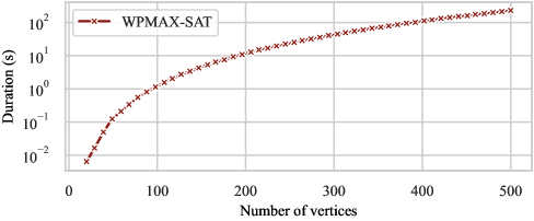
We extended the simulations in Section 5 for up to vertices, and the results are presented in Fig. 5. We observe that even at , WPMAX-SAT takes around the same time as Algorithm 2 of Akbari et al. [2022] does to solve ( s for both). Moreover, we can clearly see the exponential growth in time complexity, as expected, especially for .
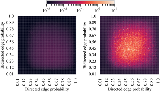
A.3 Investigating the effects of directed and bidirected edge probabilities on the performance of exact algorithms
We run experiments on varying the probabilities of directed and bidirected edges in the graph. We fix the number of vertices at and vary the probabilities of directed and bidirected edges from to in increments of . The results are presented in Fig. 6.
A.4 Investigating the effect of cost on the performance of the algorithms
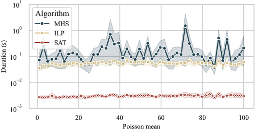
We run experiments with and costs sampled from a Poisson distributions with mean parameter ranging from to . The results are presented in Fig. 7. Interestingly, there appears to be no clear trend in the time complexity of the algorithms with respect to the mean parameter of the Poisson distribution. This suggests that the time complexity of the algorithms is not significantly affected by the cost of the vertices.
A.5 Investigating the effects of directed and bidirected edge probabilities on the performance of the heuristic algorithms
We run experiments on varying the probabilities of directed and bidirected edges in the graph. We vary from to and the probabilities of directed and bidirected edges in . The results are presented in Fig. 8. We see that our proposed heuristic algorithm consistently outperforms the heuristic algorithms of Akbari et al. [2022] for all graph sizes and edge probabilities.
Appendix B Algorithms
B.1 Pruning algorithm for finding the hedge hull
We include the algorithm for finding the hedge hull for the sake of completeness. This algorithm is adopted from Akbari et al. [2022].
B.2 SAT construction procedure for multiple districts
The procedure for constructing the SAT formula when comprises multiple districts was postponed to this section due to space limitations. This procedure is detailed below.
Appendix C Missing Proofs
C.1 Results of Section 3
See 1
Proof.
Proof of ‘if:’ Suppose hits every hedge formed for . We construct a satisfying solution for the SAT formula as follows. We begin with :
For every , define . Then for is chosen recursively as below.
-
•
Odd : if and has a directed path to in , and otherwise.
-
•
Even : if and has a bidirected path to in , and otherwise.
Next, we prove that as defined above satisfies . We consider the three types of clauses in separately:
-
•
For odd , the clause corresponds to the directed edge : if either or , then this clause is trivially satisfied. So suppose , and , which implies by construction that . Therefore, . Further, since , has a directed path to in . Then has a directed path to in because of the edge . By the construction above, , which satisfies the clause.
-
•
For even , the clause corresponds to the bidirected edge : if either or , then this clause is trivially satisfied. So suppose , and , which implies by construction that . Therefore, . Further, since , has a bidirected path to in . Then has a bidirected path to in because of the edge . By the construction above, , which satisfies the clause.
-
•
The clauses : First note that by construction, if for some , , then . That is, is a non-increasing binary-valued sequence for every . Therefore, for every , there exists at most one such that . We consider two cases separately:
-
–
There are exactly many for which there exists at least one such that . In this case, for every , there exists exactly one such that . Then for every , there exists such that , and following the argument above, . Hence, the clauses are all satisfied.
-
–
There are strictly less than many for which there exists at least one such that . Then there exist such that for every , and . Assume without loss of generality that and therefore, . If for every , then by similar arguments as the previous case, and the clauses are satisfied. So suppose for the sake of contradiction that there exists a non-empty set . Note that , since for every . Moreover, since for every and is non-increasing. Assume without loss of generality that is odd. The proof is identical in case is even. By definition, the set of vertices have a directed path to in . Moreover, the set of vertices are those vertices in that have a bidirected path to in (here we used for to be well-defined.) That is, is the connected component of in . The latter implies that every vertex in has a bidirected path to in . We proved that is a hedge formed for , and . This contradicts with intersecting with every hedge formed for .
-
–
Proof of ‘only if:’ Suppose is a satisfying solution, where for every . To prove intersects every hedge formed for , it suffices to show that there is no hedge formed for in . Assume, for the sake of contradiction, that this is not the case. That is, there exists a hedge formed for in . Suppose for some , it holds that for every . We show that for every . We consider the following two cases separately:
-
•
Even : for arbitrary such that , consider the clauses and that are in by construction for even . Since , the expression is satisfied; i.e., it evaluates to ‘true.’ The latter expression is equivalent to , which implies that . Note that were chosen arbitrarily. This implies that is equal for every , since is a connected component through bidirected edges by definition of a hedge. Finally, since by construction, for every , that equal value is . Therefore, for every such that .
-
•
Odd : the proof is analogous to the case where is even. For arbitrary such that , consider the clause . Since , the expression is satisfied; i.e., it evaluates to ‘true.’ The latter implies that if and has a directed edge to , then . Using the same argument recursively, if and has a directed ‘path’ to in , then . By construction, for every , and by definition of a hedge, every vertex has a directed path to . As a result, for every .
Since for every , , using the arguments above, by induction, for every . However, this contradicts the fact that satisfies , since includes the clauses for every . ∎
See 1
Proof.
Let be an optimizer of Eq. 1. By Proposition 1, for every , there exists that hits every hedge formed for . The set of such s is a subset of at most size of , which implies that since is optimal. If , the claim is trivial. If , then simply add empty intervention sets to to form an intervention set family with the same cost which is an optimal solution to Eq. 1. ∎
See 2
Proof.
The proof is identical to that of Theorem 1 with necessary adaptations.
Proof of ‘if:’ Suppose is a solution to Eq. 1. From Proposition 1, for every , there exists such that hits every hedge formed for . Assign and for every other , thereby satisfying every clause that includes , . So it suffices to assign values to other variables so that clauses including . Since , these clauses reduce to (see lines 16, 19, or 20.) These clauses are exactly in the form of 3-SAT clauses as in the single-district case procedure. An assignment exactly parallel to the proof of Theorem 1 satisfies these clauses.
Proof of ‘only if:’ Suppose is a satisfying solution, where for some , it holds that and for every . We show that hits every hedge formed for . Since such a exists for every , we will conclude that is feasible for Eq. 1 by Proposition 1. Finally, to show that hits every hedge formed for , note that satisfiability of all clauses containing the literal reduces to the satisfiability of (see lines 16, 19, or 20), and the same arguments as in the proof of Theorem 1 apply. ∎
C.2 Results of Section 4
See 2
Proof.
Define . First, we show that . Assume the contrary, i.e., there is a vertex . Clearly has a directed path to (a direct edge) that does not go through . This implies that , and since by definition, , . However, the latter contradicts with . Second, we note that from the third rule of do calculus [Pearl, 2009], for any . Combining the two arguments, we have the following:
| (6) |
To proceed, we will use the following proposition.
Proposition 3 (Lauritzen et al., 1990).
Let , and be disjoint subsets of vertices in a directed acyclic graph . Then d-separates from if and only if is a vertex cut between and in .
Choose in the proposition above. Since , we have that . From condition (ii) in the lemma, is a vertex cut between and in , which implies it is also a vertex cut in , as every path in the latter graph exists in . Using the proposition above, d-separates and in . This is to say, blocks all non-causal paths from to in , and it clearly has no elements that are descendants of . Therefore, satisfies the adjustment criterion of Shpitser et al. [2010] w.r.t. in . That is, the following holds:
where the expectation is w.r.t. . Choosing in Eq. 6, we get
Marginalizing out in both sides of the equation above, we have
The last step of the proof is to show that . We already showed that . For the other direction, we will use the minimality of . Suppose to the contrary that . We first show that every causal path from to goes through . Suppose not. Then take a causal path be a causal path from to . Note that has a causal path to that does not go through . By definition, , which implies , which is a contradiction. Therefore, every causal path from to goes through , and consequently, there is no causal path from to in . Clearly there is no backdoor path either. Every other path has a collider on it, and therefore is blocked by – note that none of these can be colliders in . Therefore, is d-separated from given in , which contradicts the minimality of w.r.t. the third rule of do calculus. This shows , completing the proof. ∎
See 3
Proof.
For the first part, using Lemma 2, it suffices to show that is a vertex cut between and in . Suppose not. That is, there exists a path from to in that does not pass through any member of . Let represent this path, where and . We construct a corresponding path in as follows. The first vertex on is , which corresponds to the first vertex on , . We then walk along and add a path to corresponding to each edge we traverse on as follows. Consider this edge to be – for instance, the first edge would be . By definition of , for every pair of adjacent vertices on the path , one of the following holds: (i) in , (ii) in , or (iii) and have a common child in . In case (i), we add . In case (ii), we add . Finally, in case (iii), we add to . We continue this procedure until we traverse all edges on . The last vertex on is , as x has no children in . Finally we add to this path, as and are always connected by construction. Note that by construction of , any vertex that appears with index has a parent in in , and therefore is not a member of . Hence, does not intersect with . Further, does not intersect with either, as none of the vertices appearing on correspond to . This is to say that , which is the solution obtained by Algorithm 1 in line 10, does not cut the path . This contradicts with being a vertex cut.
For the second part, let be so that is a vertex cut between and in , and induces a lower cost than ; that is, . Define . Clearly, the cost of is equal to , which is lower than the cost of minimum vertex cut found in line 10 of Algorithm 1. It suffices to show that is also a vertex cut between and in to arrive at a contradiction. Suppose not; that is, there is a path on that does not intersect. None of the vertices with index on belong to , and none of the vertices with index belong to . Analogous to the first part, we construct a corresponding path – this time in . The starting vertex on is , which corresponds to , the initial vertex on . Let us imagine a cursor on . We then sequentially build by traversing as follows. We always look at sequences starting with (where the cursor is located): when the sequence is of the form or , we add to , and move the cursor to ; however, when the sequence is of the form , we add to and move the cursor to . By construction of , no other sequence is possible – note that there are no edges between and or and where and are distinct. Since none of the vertices with index on belong to , in the first case, the corresponding edge or is present in and consequently, the edge is present in ; and in the latter case, both edges and are present in and consequently, the edge is present in . is therefore a path between and in . Notice that by construction, only those vertices appear on that their corresponding vertex with index appears on – the cursor always stays on vertices with index . As argued above, none of such vertices belong to , which means does not intersect with which is a path from to in . This contradicts with being a vertex cut. ∎
C.2.1 Proof of Remark 4
Proof.
Since the algorithms are run in the hedge hull of , assume without loss of generality that , i.e., is the hedge hull of . From Theorem 3, Algorithm 1 finds the optimal (minimum-cost) intervention such that there exists a set that is a vertex cut between and in . To prove that the cost of the solution returned by Algorithm 1 is always smaller than or equal to that of heuristic algorithm 1 proposed by Akbari et al. [2022], it suffices to show that the solution of their algorithm is a feasible point for the statement above. That is, denoting the output of heuristic algorithm 1 in Akbari et al. [2022] by , we will show that there exist sets such that it is a vertex cut between and in .
Heuristic algorithm 1: This algorithm returns an intervention set such that there is no bidirected path from to in . We claim satisfies the criterion above. To prove this, consider an arbitrary path between and in . If there is an observed vertex on , this vertex is included in and separates the path. So it suffices to show that there is no path between and in where all the intermediate vertices on correspond to unobserved confounders. Suppose there is. That is, , where and are unobserved. Since is not connected to in , it must be the case that any and have a common child in . This is to say, there is a path in , which corresponds to the bidirected path in . This contradicts with the fact that there is no bidirected path between and in . ∎
C.3 Results in the appendices
Lemma 3.
For any district , the function is submodular.
Proof.
Take two distinct vertices and an arbitrary set . It suffices to show that
By definition, the right hand side is the number of hedges formed for such that . Similarly, the left hand side counts the number of hedges formed for such that . The inequality holds because the set of hedges counted by the left hand side is a subset of that on the right hand side. ∎
Proposition 4.
The combinatorial optimization of Eq. 2 is equivalent to the following unconstrained submodular optimization problem.
| (7) |
Proof.
The submodularity of the objective function follows from Lemma 3. To show the equivalence of the two optimization problems, we show that a maximizer of Eq. 7 (i) hits every hedge formed for , and (ii) has the optimal cost among such sets.
Proof of ‘(i):’ Note that if and only if there are no hedges formed for in , or equivalently, hits every hedge formed for . So it suffices to show that for every maximizer of Eq. 7. To this end, first note that
which implies that
On the other hand, clearly , which combined with the inequality above implies . Since , it is only possible that .
Proof of ‘(ii):’ We showed that . So maximizes among all those such that . Since the denominator is a constant, this is equivalent to minimizing among all those that hit all the hedges formed for , which matches the optimization of Eq. 2. ∎
Appendix D Alternative Formulations
D.1 Min-cost intervention as a submodular function maximization problem
In this Section, we reformulate the minimum-cost intervention design as a submodular optimization problem. Submodular functions exhibit a property akin to diminishing returns: the incremental gain from adding an element to a set decreases as the set grows [Nemhauser et al., 1978].
Definition 5.
A function is submodular if for all and , we have that .
Given an ADMG a district in , and an arbitrary set , we define as the negative count of hedges formed for in . See 3 Note that , where , and is an arbitrary constant, is also submodular as the second component is a modular function (similar definition as in 5 only with equality instead of inequality.). See 4
D.2 Min-cost intervention as an RL problem
We model the MCID problem given a graph and , as a Markov decision process (MDP), where a vertex is removed in each step until there are no hedges left. The goal is to minimize the cost of the removed vertices (i.e., intervention set). Naturally, the action space is the set of vertices, and the state space is the set of all subsets of . More precisely, let and denote the state and the action of the MDP at iteration , respectively. Then, is the hedge hull for from the remaining vertices at time , and action is the vertex that will be removed from in that iteration. Consequently, the state transition due to action is . The immediate reward of selecting action at state will be the negative of the cost of removing (i.e., intervening on) , given by
The MDP terminates when there are no hedges left and the hedge hull of the remaining vertices is empty (i.e., ). The goal is to find a policy that maximizes sum of the rewards until the termination of the MDP. Formally, the goal is to solve
where and is the time step at which the MDP terminates (i.e., ).