Blind Bistatic Radar Parameter Estimation
in Doubly-Dispersive Channels

Abstract

We propose a novel method for blind bistatic radar parameter estimation (RPE), which enables integrated sensing and communications (ISAC) by allowing passive (receive) base stations (BSs) to extract radar parameters (ranges and velocities of targets), without requiring knowledge of the information sent by an active (transmit) BS to its users. The contributed method is formulated with basis on the covariance of received signals, and under a generalized doubly-dispersive channel model compatible with most of the waveforms typically considered for ISAC, such as orthogonal frequency division multiplexing (OFDM), orthogonal time frequency space (OTFS) and affine frequency division multiplexing (AFDM). The original non-convex problem, which includes an $\ell_{0}$-norm regularization term in order to mitigate clutter, is solved not by relaxation to an $\ell_{1}$-norm, but by introducing an arbitrarily-tight approximation then relaxed via fractional programming (FP). Simulation results show that the performance of the proposed method approaches that of an ideal system with perfect knowledge of the transmit signal covariance with an increasing number of transmit frames.

I Introduction

Within the recently explored paradigms of enabling technologies for B5G and 6G networks, integrated sensing and communications (ISAC) is one of the fundamental pillars which aims to combine and consolidate the presently separate areas of radar sensing and communications which is expected to significantly improve the performance and efficiency of the system [1, 2, 3]. One of the most commonly addressed ISAC approaches is the enabling of sensing functionalities via integration into wireless communications systems [4, 5, 6], referred to as communication-centric (CC)-ISAC.

There are many candidate digital modulation schemes investigated for CC-ISAC systems [7, 8], such as orthogonal frequency division multiplexing (OFDM) [9], orthogonal time frequency space (OTFS) [10] and affine frequency division multiplexing (AFDM) [11] waveforms in which the latter is currently considered to be the most promising, as it was shown to outperform OFDM and OTFS in high-mobility scenarios in terms of bit error rate (BER) and modulation complexity, respectively, while achieving an optimal diversity order in doubly-dispersive channels [12, 13].

Unfortunately, CC-ISAC systems typically consider the monostatic case of radar parameter estimation (RPE), whereby estimation occurs at the actively transmitting base station (BS), i.e., at the colocated transmitter and receiver, via the reflected echoes of the transmit signal, which implies: a) the need for costly full-duplex (FD) hardware [14] or sophisticated self-interference cancellation (SIC) mechanisms [15], and b) full knowledge of the transmit signal for RPE.

A bistatic CC-ISAC system, where the transmitter (henceforth referred to as the active BS) and receiver (henceforth referred to as the bistatic BS) are distributed in space, mitigates the latter problem, but introduces the challenge that the information embedded in the transmit signal is instantaneously unknown at the bistatic BS conducting RPE. While the fundamental idea of employing target sensing at a secondary (locally distinct) bistatic receiver resonates with passive radar [16, 17, 18], this technique is not subject to the blindness problem as the reference signal (pilots) is deterministically known and exploited.

To circumvent this issue, initial work on bistatic ISAC [19] utilizes a cooperative bistatic BS topology connected via a fronthaul for RPE. While the simulation results demonstrate effective ISAC performance, the method would in reality be subject to degradation due to imperfection in the fronthaul, which may introduce relative delays and distortion in the signals utilized by the bistatic BS. Another relevant state-of-the-art (SotA) work is a novel sensing-aided channel estimation method proposed for AFDM in [20], which can be interpreted as a variation of bistatic ISAC. However, this technique still makes use of a preamble (pilots) for sensing and the resulting non-blind framework considers a static scattering environment, where only range estimation is performed.

Motivated by the above, we consider an alternative blind bistatic CC-ISAC scenario, in which the bistatic BS has no knowledge of the information transmitted by the active BS. For such a scenario, we develop our solution under an AFDM setting, while offering straightforward generalization to the OFDM and OTFS waveforms, thanks to the doubly-dispersive channel model utilized [8]. In particular, we focus on bistatic RPE, where a bistatic BS receives both the line-of-sight (LoS) signal transmitted by an active BS, as well as non-LoS (NLoS) signals reflected by objects/targets in the surrounding. As will be shown, the a-priori knowledge of the effective channel structure is actually sufficient for the sensing operation, $i.e.,$ RPE can be performed by exploiting the channel structure without requiring the knowledge or seperate estimation of the transmit signal. Trivially, this bistatic ISAC approach requires no SIC, and can be considered an enabler of CC-ISAC.

$${\mathbf{\Phi}_{p}\triangleq\text{diag}\Big{(}[\overbrace{e^{-j2\pi\phi_{\mathrm{CP}}(\ell_{p})},e^{-j2\pi\phi_{\mathrm{CP}}(\ell_{p}-1)},\dots,e^{-j2\pi\phi_{\mathrm{CP}}(2)},e^{-j2\pi\phi_{\mathrm{CP}}(1)}}^{\ell_{p}\;\text{terms}},\overbrace{1,1,\dots,1,1}^{N-\ell_{p}\;\text{ones}}]\Big{)}\in\mathbb{C}^{N\times N}.\vspace{-5ex}}$$ (3)

$$\bm{\Omega}\triangleq\text{diag}\Big{(}[1,e^{-j2\pi/N},\dots,e^{-j2\pi(N-2)/N},e^{-j2\pi(N-1)/N}]\Big{)}\in\mathbb{C}^{N\times N}.$$ (4)

The proposed method leverages multiple frames (transmissions) from an active BS, and computes a sample covariance matrix at the bistatic BS from the received signals. A modified version of this sample covariance matrix, along with a purpose-built dictionary matrix only dependent on the channel grid structure, is then used to formulate a novel sparse recovery problem, which in turn is used to estimate target ranges and velocities via an $\ell_{0}$-norm regularization leveraging fractional programming (FP). The proposed bistatic RPE is performed with a fully blind assmption, with no instantaneous knowledge of the transmit signal at the receive bistatic BS or the total number of targets in the surrounding.

The rest of the paper is structured as follows:

• A concise system model of the doubly-dispersive scattering channel and the signal model of the AFDM waveform is provided in Section II.

• The proposed blind bistatic RPE method including relevant formulations and an original optimization problem is presented in Section III, with the solution of the formulated problem provided in Algorithm 1.

• Numerical simulations and analysis is provided in Section IV, which prove the effectiveness of the proposed blind bistatic CC-ISAC technique.

II System Model

Consider an ISAC scenario composed of one downlink transmitter (active BS), one passive receiver (bistatic BS) and $P$ significant scatterers in the environment. As illustrated in Figure 1, there is one LoS signal path between the active BS and the bistatic BS, in addition to the $P$ echo (scattered) NLoS signal paths from each target. Note that any number of the $P$ environment scatterers may be communications user equipments (UEs) receiving the downlink signal, but are still considered targets from the perspective of the bistatic BS.

II-A Doubly-Dispersive Channel Model

We consider the doubly-dispersive wireless channel [21, 8] to model the ISAC scenario with one LoS and $P$ NLoS propagation paths, whose time domain (TD) channel impulse response function $h(t,\tau)$ in the continuous time-delay domain is described by

$$h(t,\tau)\triangleq\sum_{p=0}^{P}h_{p}\cdot e^{j2\pi\nu_{p}t}\cdot\delta(\tau-\tau_{p}),\vspace{-0.5ex}$$ (1)

where $p=0$ corresponds to the LoS path and $p\in\{1,\cdots\!,P\}$ corresponds to the NLoS path from each $p$-th target; $h_{p}\in\mathbb{C}$ is the $p$-th channel fading coefficient; $\tau_{p}\in[0,\tau_{\text{max}}]$ is the $p$-th path delay bounded by the maximum delay $\tau_{\text{max}}$; $\nu_{p}\in[-\nu_{\text{max}},\nu_{\text{max}}]$ is the $p$-th Doppler shift bounded by the maximum Doppler shift $\nu_{\text{max}}$ and $\delta(\,\cdot\,)$ is the unit impulse function.

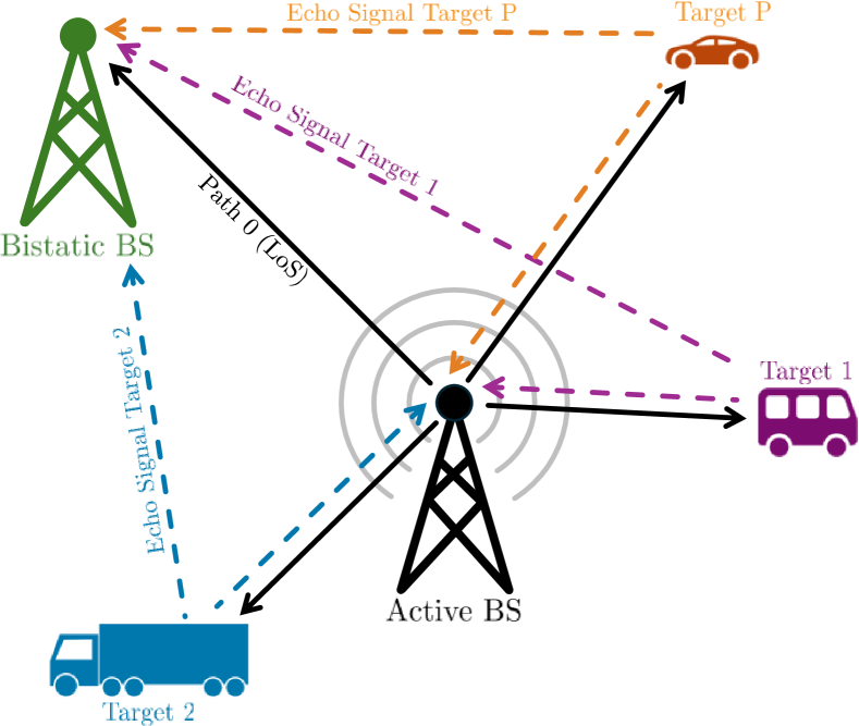
Figure 1: Illustration of an ISAC system showing the 1 LoS path and $P$ target echo paths between the active BS and the passive bistatic BS.

Given an arbitrary time-domain transmit signal $s(t)$, the received signal $r(t)\triangleq s(t)*h(t,\tau)+w(t)$ where $w(t)$ is the additive white Gaussian noise (AWGN), can be concisely described by a discrete circular convolutional form [8] by sampling at the frequency $f_{\mathrm{S}}$,

$$\mathbf{r}=\!\bigg{(}\sum_{p=0}^{P}h_{p}\!\cdot\mathbf{\Phi}_{p}\!\cdot\bm{\Omega}^{f_{p}}\!\cdot\!\mathbf{\Pi}^{\ell_{p}}\!\bigg{)}\!\cdot\mathbf{s}+\mathbf{w}=\bm{\Psi}\mathbf{s}+\mathbf{w}\;\in\mathbb{C}^{N\times 1},\vspace{-1ex}$$ (2)

where $\mathbf{r}\in\mathbb{C}^{N\times 1}$, $\mathbf{s}\in\mathbb{C}^{N\times 1}$ and $\mathbf{w}\in\mathbb{C}^{N\times 1}$ are the transmit, received and AWGN signal vectors consisting of $N$ samples, respectively; $\bm{\Psi}\in\mathbb{C}^{N\times N}$ is the effective circular convolutional channel matrix, $\mathbf{\Phi}_{p}\in\mathbb{C}^{N\times N}$ described in equation (3) is a diagonal matrix capturing the effect of the cyclic prefix (CP) phase with $\phi_{\mathrm{CP}}(n)$ denoting the waveform-dependent phase function [8] on the sample index $n\in\{0,\cdots,N-1\}$; $\bm{\Omega}\in\mathbb{C}^{N\times N}$ described in equation (4) is a diagonal matrix containing the $N$ complex roots of unity; and $\mathbf{\Pi}\in\{0,1\}^{N\times N}$ is the forward cyclic shift matrix, with elements given by

$$\pi_{i,j}=\delta_{i,j+1}+\delta_{i,j-(N-1)}\;\;\text{where}\;\;\delta_{ij}\triangleq\begin{cases}0&\text{if }i\neq j,\\ 1&\text{if }i=j.\end{cases}$$ (5)

$$\bm{\varPhi}_{p}\triangleq\text{diag}\Big{(}[\overbrace{e^{-j2\pi c_{1}(N^{2}-2N\ell_{p})},e^{-j2\pi c_{1}(N^{2}-2N(\ell_{p}-1))},\cdots,e^{-j2\pi c_{1}(N^{2}-2N)}}^{\ell_{p}\;\text{terms}},\overbrace{1,1,\dots,1,1}^{N-\ell_{p}\;\text{ones}}]\Big{)}\in\mathbb{C}^{N\times N}.\vspace{-1ex}$$ (10)

Furthermore, the roots-of-unity matrix $\bm{\Omega}$ and the forward cyclic shift matrix $\mathbf{\Pi}$ are respectively exponentiated to the power of $f_{p}\triangleq\frac{N\nu_{p}}{f_{\mathrm{S}}}$ and $\ell_{p}\triangleq\frac{\tau_{p}}{T_{\mathrm{S}}}$, which are the normalized digital Doppler frequency and the normalized delay of the $p$-th path, respectively, where $T_{\mathrm{S}}\triangleq\frac{1}{f_{\mathrm{S}}}$ is the delay resolution. The two matrix exponentiations capture the effect of the Doppler shift and the integer delay in the circular convolutional channel given in equation (2).

II-B AFDM Signal Input-Output Relationship

The doubly-dispersive channel model in equation (2) is derived for an arbitrary transmitter structure in $s(t)$, such that any waveform such as OFDM, OTFS, and AFDM can be used. Since a thorough comparison of the waveforms for ISAC is provided in [22], highlighting the superiority of the AFDM for ISAC in doubly-dispersive channels, the AFDM transmitter structure is elaborated below, and considered in this article henceforth without loss of generality (w.l.g.).

Let $\mathbf{x}\in\mathbb{C}^{N\times 1}$ denote the information vector with elements drawn from an arbitrary complex digital constellation $\mathcal{C}$, with cardinality $Q\triangleq|\mathcal{C}|$ and average symbol energy $\sigma^{2}_{X}$. The corresponding AFDM modulated transmit signal of $\mathbf{x}$ is given by its inverse discrete affine Fourier transform (IDAFT), $i.e.,$

$$\mathbf{s}_{\text{AFDM}}=(\mathbf{\Lambda}_{1}^{\mathsf{H}}\mathbf{F}_{N}^{\mathsf{H}}\mathbf{\Lambda}_{2}^{\mathsf{H}})\cdot\mathbf{x}\in\mathbb{C}^{N\times 1},$$ (6)

where $\mathbf{F}_{N}\in\mathbb{C}^{N\times N}$ denotes the $N$-point normalized discrete Fourier transform (DFT) matrix, and the two diagonal chirp matrices $\mathbf{\Lambda}_{i}$ are defined as

$$\!\!\!\!\mathbf{\Lambda}_{i}\!\triangleq\!\mathrm{diag}\Big{(}\big{[}1,\cdots\!,e^{-j2\pi c_{i}n^{2}}\!\!,\cdots\!,e^{-j2\pi c_{i}(N-1)^{2}}\big{]}\Big{)}\!\in\!\mathbb{C}^{N\times N}\!,\!\!\!$$ (7)

where the first central frequency $c_{1}$ can be selected for optimal robustness to doubly-dispersivity based on the channel statistics [13], and the second central frequency $c_{2}$ can be exploited for waveform design and applications [23, 24].

In addition, the AFDM modulated signal also requires the insertion of a chirp-periodic prefix (CPP) to mitigate the effects of multipath propagation [13] analogous to the CP in OFDM, whose multiplicative phase function for equation (3) is given by $\phi_{\mathrm{CPP}}(n)=c_{1}(N^{2}-2Nn)$ [8]. Correspondingly, the received AFDM signal vector is given by

$$\mathbf{r}_{\text{AFDM}}\triangleq\bm{\Psi}\cdot\mathbf{s}_{\text{AFDM}}+\mathbf{w}\in\mathbb{C}^{N\times 1}.$$ (8)

Then, the received signal in equation (8) is demodulated via the discrete affine Fourier transform (DAFT) to yield

$$\mathbf{y}_{\text{AFDM}}\! =\!(\mathbf{\Lambda}_{2}\mathbf{F}_{N}\mathbf{\Lambda}_{1})\cdot\mathbf{r}_{\text{AFDM}}\in\mathbb{C}^{N\times 1}$$ (9)

$$=\!(\mathbf{\Lambda}_{2}\mathbf{F}_{N}\mathbf{\Lambda}_{1})\!\cdot\!\bigg{(}\!\!~{}\!\sum_{p=0}^{P}h_{p}\!\!\cdot\!\bm{\varPhi}_{p}\!\!\cdot\!\bm{\Omega}^{f_{p}}\!\!\cdot\!\mathbf{\Pi}^{\ell_{p}}\!\!\bigg{)}\!\cdot\!(\mathbf{\Lambda}_{1}^{\mathsf{H}}\mathbf{F}_{N}^{\mathsf{H}}\mathbf{\Lambda}_{2}^{\mathsf{H}})\!\cdot\!\mathbf{x}$$

$$~{}~{}~{}+\!(\mathbf{\Lambda}_{2}\mathbf{F}_{N}\mathbf{\Lambda}_{1})\mathbf{w},$$

where $\bm{\varPhi}_{p}$ is the diagonal matrix as described in equation (10), which inherently incorporates the AFDM CPP phase function.

In light of the above, the final input-output relationship of AFDM over doubly-dispersive channels is given by

$$\mathbf{y}_{\text{AFDM}}=\mathbf{G}_{\text{AFDM}}\cdot\mathbf{x}+\tilde{\mathbf{w}}_{\text{AFDM}}\in\mathbb{C}^{N\times 1},$$ (11)

where $\tilde{\mathbf{w}}_{\text{AFDM}}\triangleq(\mathbf{\Lambda}_{2}\mathbf{F}_{N}\mathbf{\Lambda}_{1})\mathbf{w}\in\mathbb{C}^{N\times 1}$ is an equivalent AWGN vector with the same statistical properties as $\mathbf{w}$, and $\mathbf{G}_{\text{AFDM}}\in\mathbb{C}^{N\times N}$ is the effective AFDM channel defined by

$$\!\!\!\!\mathbf{G}_{\text{AFDM}}\!\triangleq\!\sum_{p=0}^{P}h_{p}\!\cdot\!(\mathbf{\Lambda}_{2}\mathbf{F}_{N}\mathbf{\Lambda}_{1})\!\!\cdot\!\!\big{(}\bm{\varPhi}_{p}\!\!\cdot\!\bm{\Omega}^{f_{p}}\!\!\cdot\!\mathbf{\Pi}^{\ell_{p}}\!\big{)}\!\!\cdot\!\!(\mathbf{\Lambda}_{1}^{\mathsf{H}}\mathbf{F}_{N}^{\mathsf{H}}\mathbf{\Lambda}_{2}^{\mathsf{H}}).\!\!\!\!$$ (12)

For the sake of completeness, the effective channels and equivalent noise of the OFDM and OTFS waveforms are provided below, which can be replaced in equation (11) w.l.g., as

$$\mathbf{G}_{\text{OFDM}}\triangleq\sum_{p=0}^{P}h_{p}\cdot\mathbf{F}_{N}\cdot(\bm{\Omega}^{f_{p}}\cdot\mathbf{\Pi}^{\ell_{p}})\cdot\mathbf{F}_{N}^{\mathsf{H}},\vspace{-1ex}$$ (13a)

$$\tilde{\mathbf{w}}_{\text{OFDM}}\triangleq\mathbf{F}_{N}\cdot\mathbf{w}\in\mathbb{C}^{N\times 1},$$ (13b)

and

$$\mathbf{G}_{\text{OTFS}}\triangleq\sum_{p=0}^{P}h_{p}\cdot(\mathbf{F}_{M}\otimes\mathbf{I}_{K})\cdot(\bm{\Omega}^{f_{p}}\cdot\mathbf{\Pi}^{\ell_{p}})\cdot(\mathbf{F}_{M}^{\mathsf{H}}\otimes\mathbf{I}_{K}),$$ (14a)

$$\tilde{\mathbf{w}}_{\text{OTFS}}\triangleq(\mathbf{F}_{M}\otimes\mathbf{I}_{K})\cdot\mathbf{w}\in\mathbb{C}^{N\times 1},$$ (14b)

where $\otimes$ denotes the Kronecker product, $M,K\in\mathbb{N}$ satisfying $N=MK$ are the two-dimensional (2D) grid dimensions of the OTFS waveform [5], and $\mathbf{I}_{M}$ is the $M\times M$ identity matrix.

III Blind Bistatic Radar Parameter Estimation

In this section, we first build a canonical sparse recovery problem by creating a sample covariance matrix leveraging a reformulation of the system model encapsulating multiple transmission frames with a discretized solution space by considering bounds on the maximum ranges/velocities of the potential targets in the surrounding. Finally, we offer two solutions for the problem: a) A naive least absolute shrinkage and selection operator (LASSO) formulation that is used to initialize the proposed regularization and b) a novel non-convex problem formulation which is solved via the introduction of an arbitrarily-tight approximation relaxed using FP.

III-A System Model Reformulation

First, let us express the effective input-output relationships given in equation (11) in the following form

$$\mathbf{y}=\Big{(}\underbrace{\sum_{p=0}^{P}h_{p}\cdot\mathbf{\Gamma}_{p}}_{\triangleq\mathbf{G}}\Big{)}\cdot\mathbf{x}+\tilde{\mathbf{w}}\in\mathbb{C}^{N\times 1},$$ (15)

where the matrices $\mathbf{\Gamma}_{p}$ capture the long-term DD statistics of the channel comprising of the coefficients with the delay and Doppler shifts, and the variables have been expressed for a general waveform in light of equations (12), (13) and (14).

The equivalent system in equation (15) without the extrinsic summation on the path index $p$ can be obtained as

$$\mathbf{y}=\mathbf{H}\cdot\mathbf{\Gamma}\cdot\mathbf{x}+\tilde{\mathbf{w}}\in\mathbb{C}^{N\times 1},$$ (16)

where the channel coefficient matrix $\mathbf{H}$ and the long-term DD matrix $\mathbf{\Gamma}$ are respectively defined as

$$\mathbf{H}\!\triangleq\!\left[\begin{array}[]{@{\,}c@{\,}c@{\,}c@{\,}c@{\,}c@{\,}c@{\,}c@{\,}c@{\,}c@{\,}c@{\,}c@{\,}}h_{0}&\cdots&0&h_{1}&\cdots&0&h_{P}&\cdots&0\\[-4.30554pt] \vdots&\ddots&\vdots&\vdots&\ddots&\vdots&\vdots&\ddots&\vdots\\[-1.07639pt] 0&\cdots&h_{0}&0&\cdots&h_{1}&0&\cdots&h_{P}\\ \end{array}\right]\in\mathbb{C}^{N\times N(P+1)},$$ (17)

and

$$\mathbf{\Gamma}\triangleq\begin{bmatrix}\mathbf{\Gamma}_{0}&\mathbf{\Gamma}_{1}&\cdots&\mathbf{\Gamma}_{P}\end{bmatrix}^{\mathsf{T}}\in\mathbb{C}^{N(P+1)\times N}.$$ (18)

Finally, considering a stream of $T$ transmitted frames, where each frame refers to a single vector $\mathbf{x}\in\mathbb{C}^{N\times 1}$, yields

$$\mathbf{Y}=\mathbf{H}\cdot\mathbf{\Gamma}\cdot\mathbf{X}+\tilde{\mathbf{W}}\in\mathbb{C}^{N\times T},$$ (19)

where

$$\mathbf{Y}\triangleq[\mathbf{y}_{1},\dots,\mathbf{y}_{2},\dots,\mathbf{y}_{T}]\in\mathbb{C}^{N\times T},$$ (20a)

$$\mathbf{X}\triangleq[\mathbf{x}_{1},\dots,\mathbf{x}_{2},\dots,\mathbf{x}_{T}]\in\mathbb{C}^{N\times T},$$ (20b)

$$\tilde{\mathbf{W}}\triangleq[\tilde{\mathbf{w}}_{1},\dots,\tilde{\mathbf{w}}_{2},\dots,\tilde{\mathbf{w}}_{T}]\in\mathbb{C}^{N\times T}.$$ (20c)

III-B Proposed Problem Formulation

To facilitate a completely blind estimation which implies the availability of only the received signals, we leverage the sample covariance matrix described by

$$\mathbf{Y}\cdot\mathbf{Y}^{\mathsf{H}}=\mathbf{H}\cdot\mathbf{\Gamma}\cdot\mathbf{X}\cdot\mathbf{X}^{\mathsf{H}}\cdot\mathbf{\Gamma}^{\mathsf{H}}\cdot\mathbf{H}^{\mathsf{H}}+\mathbf{H}\cdot\mathbf{\Gamma}\cdot\mathbf{X}\cdot\tilde{\mathbf{W}}^{\mathsf{H}}$$

$$~{}~{}\;\!+\tilde{\mathbf{W}}\cdot\mathbf{X}^{\mathsf{H}}\cdot\mathbf{\Gamma}^{\mathsf{H}}\cdot\mathbf{H}^{\mathsf{H}}+\tilde{\mathbf{W}}\cdot\tilde{\mathbf{W}}^{\mathsf{H}}\in\mathbb{C}^{N\times N}.$$

Provided that a normalized symbol constellation $\mathcal{C}$ and a sufficiently large $T$ is used, equation (III-B) can be rewritten as

$$\mathbf{Y}\!\cdot\!\mathbf{Y}^{\mathsf{H}}\approx T(\sigma^{2}_{X}\cdot\mathbf{H}\cdot\mathbf{\Gamma}\cdot\mathbf{\Gamma}^{\mathsf{H}}\cdot\mathbf{H}^{\mathsf{H}}+\sigma^{2}_{W}\cdot\mathbf{I}_{N})\in\mathbb{C}^{N\times N},$$ (22)

where $\sigma^{2}_{W}$ is the variance of an arbitrary column in $\tilde{\mathbf{W}}$.

Setting $\sigma^{2}_{X}=1$ w.l.g., equation (III-B) can also be exactly described as

$$\underset{T\rightarrow\infty}{\text{lim}}\underbrace{\frac{1}{T}\cdot\mathbf{Y}\!\cdot\!\mathbf{Y}^{\mathsf{H}}-\sigma^{2}_{W}\cdot\mathbf{I}_{N}}_{\triangleq\tilde{\mathbf{R}}_{Y}\in\mathbb{C}^{N\times N}}=\underbrace{\mathbf{H}\cdot\mathbf{\Gamma}\cdot\mathbf{\Gamma}^{\mathsf{H}}\cdot\mathbf{H}^{\mathsf{H}}}_{\text{perfect covariance matrix}}\in\mathbb{C}^{N\times N},$$ (23)

where we have implicitly defined the modified sample covariance matrix $\tilde{\mathbf{R}}_{Y}\in\mathbb{C}^{N\times N}$.

Next, using the definition for $\mathbf{H}\cdot\mathbf{\Gamma}$ and equation (15), equation (23) can be expressed in terms of two sums as

$$\tilde{\mathbf{R}}_{Y}=\bigg{(}\sum_{p=0}^{P}h_{p}\cdot\mathbf{\Gamma}_{p}\bigg{)}\!\cdot\!\bigg{(}\sum_{p=0}^{P}h_{p}\cdot\mathbf{\Gamma}_{p}\bigg{)}^{\!\!\mathsf{H}}\in\mathbb{C}^{N\times N}.$$ (24)

Defining $\mathbf{H}_{\mathrm{G}}\triangleq\mathbf{h}\cdot\mathbf{h}^{\mathsf{H}}$ with $\mathbf{h}\triangleq[h_{0},\dots,h_{p},\dots,h_{P}]^{\mathsf{T}}$, the $(p,q)$-th element can be represented by $\mathbf{H}_{\mathrm{G}}(p,q)$. Using this definition, simplifying equation (24) yields

$$\tilde{\mathbf{R}}_{Y}=\sum_{p=0}^{P}\sum_{q=0}^{P}\mathbf{H}_{\mathrm{G}}(p,q)\cdot\underbrace{\mathbf{\Gamma}_{p}\cdot\mathbf{\Gamma}_{q}^{\mathsf{H}}}_{\tilde{\mathbf{\Gamma}}_{p,q}}\in\mathbb{C}^{N\times N}.$$ (25)

Since each distinct matrix $\mathbf{\Gamma}_{p}$ is unitary, the matrices $\tilde{\mathbf{\Gamma}}_{p,q}$ in equation (25) amount to identity matrices of size $N\times N$ when $p\!=\!q$, resulting in uniqueness ($i.e.,$ useful distinct information for RPE) only for $p\!\neq\!q$. Since this uniqueness is preserved in mostly diagonal/off-diagonal elements in these sparse matrices and to alleviate the computational burden of using $N\times N$ matrices, we consider a summation of the rows of equation (25) as

$$\bar{\mathbf{r}}_{Y}\;\triangleq\tilde{\mathbf{R}}_{Y}\!\cdot\!\mathbf{1}_{N}=\!\sum_{p=0}^{P}\sum_{q=0}^{P}\mathbf{H}_{\mathrm{G}}(p,q)\cdot\!\!\!\underbrace{\tilde{\mathbf{\Gamma}}_{p,q}\!\cdot\!\mathbf{1}_{N}}_{\triangleq\mathbf{e}_{p,q}\in\mathbb{C}^{N\times 1}}\!\!\!=\mathbf{E}\!\cdot\!\text{vec}(\mathbf{H}_{\mathrm{G}}),$$

where $\mathbf{1}_{N}$ denotes an $N\times 1$ vector of ones, $\text{vec}(\mathbf{H}_{\mathrm{G}})$ denotes the column-wise vectorized form of $\mathbf{H}_{\mathrm{G}}$, and the dictionary matrix $\mathbf{E}\in\mathbb{C}^{N\times(P+1)^{2}}$ is defined as

$$\mathbf{E}\triangleq\big{[}\mathbf{e}_{0,0},\cdots\!,\mathbf{e}_{0,P},\cdots\!,\mathbf{e}_{P,0},\cdots\!,\mathbf{e}_{P,P}\big{]}\in\mathbb{C}^{N\times(P+1)^{2}}.$$ (27)

Next, we follow a similar strategy in [26, 22] to sparsify the system by decoupling and discretizing the path-wise doubly-dispersive channel model, i.e., reformulating the delay-Doppler representation of equation (1) given by [8]

$$h(\tau,\nu)=\sum_{p=0}^{P}h_{p}\!\cdot\!\delta(\tau-\tau_{p})\!\cdot\!\delta(\nu-\nu_{p}),$$ (28)

into

$$h(\tau,\nu)=\sum_{k=0}^{K_{\tau}-1}\sum_{d=0}^{D_{\nu}-1}h_{k,d}\!\cdot\!\delta(\tau-\tau_{k})\!\cdot\!\delta(\nu-\nu_{d}),$$ (29)

where $K_{\tau}\triangleq\mathrm{max}(\ell_{p})$ and $D_{\nu}\triangleq\mathrm{max}(f_{p})$ are respectively the maximum normalized delay spread and maximum digital normalized Doppler spread indices satisfying the underspread assumption $K_{\tau}<\!<N$ and $D_{\nu}<\!<N$.

Consequently, the normalized delay and Doppler shift parameters are decoupled from each $p$-th path and instead into a sparsified delay-Doppler grid, such that the auxiliary channel matrix is instead described by $\bar{\mathbf{H}}_{\mathrm{G}}\triangleq\bar{\mathbf{h}}\cdot\bar{\mathbf{h}}^{\mathsf{H}}$ with $\bar{\mathbf{h}}\triangleq[h_{0},\cdots\!,h_{k\cdot d},\cdots\!,h_{(K_{\tau}-1)\cdot(D_{\nu}-1)}]^{\mathsf{T}}$, consequently yielding

$$\bar{\mathbf{r}}_{Y}=\bar{\mathbf{E}}\cdot\text{vec}(\bar{\mathbf{H}}_{\mathrm{G}})\in\mathbb{C}^{N\times 1},$$ (30)

with the modified dictionary matrix $\bar{\mathbf{E}}\in\mathbb{C}^{N\times K_{\tau}^{2}D_{\nu}^{2}}$ adopting distinct values for the delay and Doppler indices given by

$$\bar{\mathbf{E}}\triangleq\big{[}\bar{\mathbf{e}}_{0,0},\cdots\!,\bar{\mathbf{e}}_{0,(K_{\tau}-1)\cdot(D_{\nu}-1)},\cdots$$

$$\cdots\!,\bar{\mathbf{e}}_{(K_{\tau}-1)\cdot(D_{\nu}-1),0},\cdots\!,\bar{\mathbf{e}}_{(K_{\tau}-1)\cdot(D_{\nu}-1),(K_{\tau}-1)\cdot(D_{\nu}-1)}\big{]},$$

with $\bar{\mathbf{e}}_{k\cdot d,k^{\prime}\cdot d^{\prime}}\in\mathbb{C}^{N\times 1}$ correspondingly defined as

$$\bar{\mathbf{e}}_{k\cdot d,k^{\prime}\cdot d^{\prime}}\triangleq (\mathbf{\Lambda}_{2}\mathbf{F}_{N}\mathbf{\Lambda}_{1})\cdot(\bar{\bm{\varPhi}}_{k}\cdot\bar{\bm{\Omega}}^{f_{d}}\cdot\bar{\mathbf{\Pi}}^{\ell_{k}})$$

$$\cdot(\bar{\bm{\varPhi}}_{k^{\prime}}\cdot\bar{\bm{\Omega}}^{f_{d^{\prime}}}\cdot\bar{\mathbf{\Pi}}^{\ell_{k^{\prime}}})^{\mathsf{H}}\cdot(\mathbf{\Lambda}_{1}^{\mathsf{H}}\mathbf{F}_{N}^{\mathsf{H}}\mathbf{\Lambda}_{2}^{\mathsf{H}})\cdot\mathbf{1}_{N},$$ (32)

where $\bar{\bm{\varPhi}}_{k}$, $\bar{\bm{\Omega}}^{f_{d}}$, and $\bar{\mathbf{\Pi}}^{\ell_{k}}$ are computed via equations (10), (4) and (5), respectively, with the indices $\ell_{p}$ and $f_{p}$ replaced by their corresponding location on the discrete grid as $\ell_{k}$ and $f_{d}$ for each corresponding normalized delay and Doppler index of the two corresponding grid points $(k,d)$ and $(k^{\prime},d^{\prime})$.

III-C Proposed Solution via the $\ell_{0}$-norm Approximation

Observing equation (30), it is most likely that $N<\!<K_{\tau}^{2}D_{\nu}^{2}$ for moderate grid resolutions and $\text{vec}(\bar{\mathbf{H}}_{\mathrm{G}})$ is sparse, such that the estimation of $\bar{\mathbf{H}}_{\mathrm{G}}$ becomes an underdetermined linear problem, resulting in an infeasible solution via a simple least squares formulation. Therefore, relaxed approaches such as the LASSO [27] can be leveraged to exploit the intrinsic sparsity of $\bar{\mathbf{H}}_{\mathrm{G}}$ and obtain a feasible solution via the optimization problem described by

$$\underset{\bar{\mathbf{H}}_{\mathrm{G}}\in\mathbb{C}^{K_{\tau}D_{\nu}\times K_{\tau}D_{\nu}}}{\text{minimize}}\lVert\bar{\mathbf{r}}_{Y}-\bar{\mathbf{E}}\cdot\text{vec}(\bar{\mathbf{H}}_{\mathrm{G}})\rVert^{2}_{2}\,+\,\beta\cdot\lVert\text{vec}(\bar{\mathbf{H}}_{\mathrm{G}})\rVert_{1},$$ (33)

where $\lVert\cdot\rVert_{q}$ denotes the $\ell_{q}$-norm, and $\beta\in\mathbb{R}^{+}$ is a sparsity-enforcing penalty parameter.

However, to complement the full structure of the problem in equation (30), the complete optimization to solve it without the $\ell_{1}$-norm relaxation of the LASSO can be formulated as

$$\underset{\bar{\mathbf{H}}_{\mathrm{G}}\in\mathbb{C}^{K_{\tau}D_{\nu}\times K_{\tau}D_{\nu}}}{\text{minimize}} \lVert\bar{\mathbf{r}}_{Y}-\bar{\mathbf{E}}\cdot\text{vec}(\bar{\mathbf{H}}_{\mathrm{G}})\rVert^{2}_{2},$$ (34a)

subject to $$\bar{\mathbf{H}}_{\mathrm{G}}\succcurlyeq 0,$$ (34b)

$$\lVert\text{vec}(\bar{\mathbf{H}}_{\mathrm{G}})\rVert_{0}=(P+1)^{2},$$ (34c)

$$\hskip 0.86108pt\mathrm{rank}(\bar{\mathbf{H}}_{\mathrm{G}})=1,$$ (34d)

where the first constraint intrinsically forces constructively coupled solutions, the second constraint enforces the sparsity of the solution, and the third constraint trivially results from the definition $\bar{\mathbf{H}}_{\mathrm{G}}\triangleq\bar{\mathbf{h}}\cdot\bar{\mathbf{h}}^{\mathsf{H}}$.

As a fully blind sensing scenario cannot assume prior knowledge of the actual number of paths in the estimation procedure, in addition to the non-convex third constraint, equation (34) is relaxed as

$$\underset{\bar{\mathbf{H}}_{\mathrm{G}}\in\mathbb{C}^{K_{\tau}D_{\nu}\times K_{\tau}D_{\nu}}}{\text{minimize}} \lVert\bar{\mathbf{r}}_{Y}\!-\!\bar{\mathbf{E}}\cdot\text{vec}(\bar{\mathbf{H}}_{\mathrm{G}})\rVert^{2}_{2}+\eta\lVert\text{vec}(\bar{\mathbf{H}}_{\mathrm{G}})\rVert_{0},\!\!\!\!\!$$ (35a)

subject to $$\bar{\mathbf{H}}_{\mathrm{G}}\succcurlyeq 0,$$ (35b)

where $\eta\in\mathbb{R}^{+}$ denotes the weight parameter of the $\ell_{0}$-norm regularization.

The above optimization problem in equation (35) is still non-convex due to the $\ell_{0}$-norm within the objective function, and is consequently convexized via the method proposed in [29], which approximates the $\ell_{0}$-norm of an arbitrary complex vector $\mathbf{b}=[b_{1},\dots,b_{N}]^{\mathsf{T}}\in\mathbb{C}^{N\times 1}$ as

$$\lVert\mathbf{b}\rVert_{0}\approx\sum_{n=1}^{N}\frac{\lvert b_{n}\rvert^{2}}{\lvert b_{n}\rvert^{2}+\alpha}=N-\sum_{N=1}^{M}\frac{\alpha}{\lvert b_{n}\rvert^{2}+\alpha},$$ (36)

with $\alpha\in\mathbb{R}^{+}$ denoting the hyperparameter that controls the tightness of the approximation.

Applying FP [30] to the $\ell_{0}$-norm approximation in equation (36) to convexize the affine-over-convex ratios, we obtain

$$\lVert\mathbf{b}\rVert_{0}\approx N-\Bigg{(}\sum_{n=1}^{N}2\tilde{\alpha}_{n}\sqrt{\alpha}-\tilde{\alpha}_{n}^{2}\cdot\lvert b_{n}\rvert^{2}+\tilde{\alpha}_{n}^{2}\cdot\alpha\Bigg{)},$$ (37)

where $\tilde{\alpha}_{n}$ is an auxiliary variable computed from a previously estimated $\tilde{\mathbf{b}}=[\tilde{b}_{1},\dots,\tilde{b}_{N}]^{\mathsf{T}}$, via

$$\tilde{\alpha}_{n}\triangleq\frac{\sqrt{\alpha}}{\lvert\tilde{b}_{n}\rvert^{2}+\alpha},\;\forall n.$$ (38)

Consequently, using the above iterative approximation of the $\ell_{0}$-norm, the optimization problem in equation (35) can be relaxed, resulting in

$$\underset{\bar{\mathbf{H}}_{\mathrm{G}}\in\mathbb{C}^{K_{\tau}D_{\nu}\times K_{\tau}D_{\nu}}}{\text{minimize}} \hskip 11.62494pt\lVert\bar{\mathbf{r}}_{Y}\!-\!\bar{\mathbf{E}}\cdot\text{vec}(\bar{\mathbf{H}}_{\mathrm{G}})\rVert^{2}_{2}$$ (39a)

$$\hskip 15.0694pt+\eta\cdot\text{vec}(\bar{\mathbf{H}}_{\mathrm{G}})^{\mathsf{H}}\cdot\tilde{\mathbf{A}}\cdot\text{vec}(\bar{\mathbf{H}}_{\mathrm{G}}),$$

subject to $$\hskip 12.91663pt\bar{\mathbf{H}}_{\mathrm{G}}\succcurlyeq 0,$$ (39b)

where $\tilde{\mathbf{A}}\triangleq\text{diag}([\tilde{\alpha}_{1}^{2},\dots,\tilde{\alpha}_{m}^{2},\dots,\tilde{\alpha}_{M}^{2}])$.

In summary, using the received signal matrix $\mathbf{Y}$ to compute the modified sample covariance vector according to equations (23) and (III-B) and constructing the modified dictionary matrix using equation (III-B) with all the possible values of $\ell_{k}$ and $f_{d}$, we first obtain an initial solution via the LASSO formulation in equation (33) to initialize the final optimization problem. Next, the final optimization problem in equation (39) is iteratively solved to obtain a final estimate for $\bar{\mathbf{H}}_{\mathrm{G}}$.

Algorithm 1 Blind Bistatic Radar Parameter Estimation

Input: Received signal matrix $\mathbf{Y}$, dictionary matrix $\bar{\mathbf{E}}$, noise power $\sigma_{w}^{2}$, number of transmit frames $T$, maximum number of iterations $i_{\text{max}}$, optimization hyperparameters $\beta$, $\eta$ and $\alpha$.
Output: Estimated delay and Doppler shifts $\hat{\tau}_{p}$ and $\hat{\nu}_{p}$.  

1:Compute $\bar{\mathbf{r}}_{Y}$ using eqs. (23) and (III-B).

2:Obtain an initial estimate for $\bar{\mathbf{H}}_{\mathrm{G}}$ by solving the LASSO problem in eq. (33).

3:for $i=1$ to $i_{\text{max}}$ do

4:Compute the FP auxiliary matrix $\tilde{\mathbf{A}}$ via eq. (38).

5:Obtain $\bar{\mathbf{H}}_{\mathrm{G}}$ by solving the final problem in eq. (39).

6:end for

7:Compute the estimates $\hat{\tau}_{p}$ and $\hat{\nu}_{p}$ corresponding to the $(P+1)^{2}$ non-zero entries of $\bar{\mathbf{H}}_{\mathrm{G}}$ in accordance to the dictionary matrix given in eq. (III-B); $i.e.,$ match the computed indices to the dictionary matrix to find the final estimates for $\hat{\tau}_{p}$ and $\hat{\nu}_{p}$.

Finally, since the dictionary matrix built via equation (III-B) is constructed using all the possible values of $\ell_{k}$ and $f_{d}$, by associating the non-zero entries in $\bar{\mathbf{H}}_{\mathrm{G}}$ to the columns of $\bar{\mathbf{E}}$, the final estimates for $\hat{\tau}_{p}$ and $\hat{\nu}_{p}$ can be obtained.

An overview of the proposed scheme is provided in the form of a pseudo-code in Algorithm 1.

IV Performance Analysis

To evaluate the performance of the proposed blind bistatic RPE scheme, we first consider the illustration detailed in Figure 1. In such a scenario with a passive bistatic BS receiving AFDM-modulated signals from an active BS, we consider blind RPE at the bistatic BS.

The chosen performance metric is the classical root mean square error (RMSE), which is defined as

$$\Upsilon\triangleq||\hat{\vartheta}_{p}-\vartheta_{p}||^{2}_{2},\vspace{-0.5ex}$$ (40)

where $\vartheta_{p}$ denotes a given radar parameter (range or velocity) and $\hat{\vartheta}_{p}$ its estimate.

In addition, the signal-to-noise ratio (SNR) for RPE is defined similarly to [11] as

$$\text{SNR}\triangleq\frac{(P+1)\cdot\sigma_{h}^{2}}{\sigma_{W}^{2}},\vspace{-0.5ex}$$ (41)

where $\sigma_{h}^{2}$ denotes the power of the channel coefficient $h_{p}$ associated with a given $p$-th target, as defined in equation (1), already incorporating the LoS path.

We show, in Figure 2 and Figure 3, results for a situation with one LoS signal from the transmitting active BS which is assumed to be static and situated at a distance of $3.75$ m from the bistatic BS and one NLoS reflected signal from a target ($i.e.,P=1$) at a range of $15$ m moving with a velocity of $37$ m/s towards the bistatic BS.

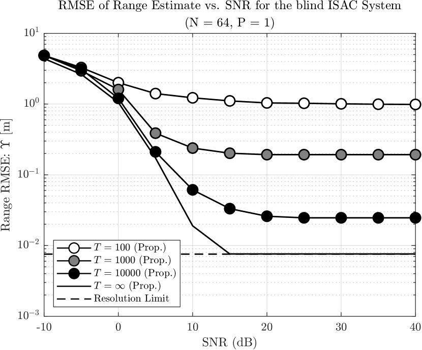
Figure 2: Range RMSE versus SNR performance of the proposed blind bistatic RPE scheme over the AFDM waveform with a single LoS signal from the active (static) BS and one NLoS echo signal from a target in the surrounding.

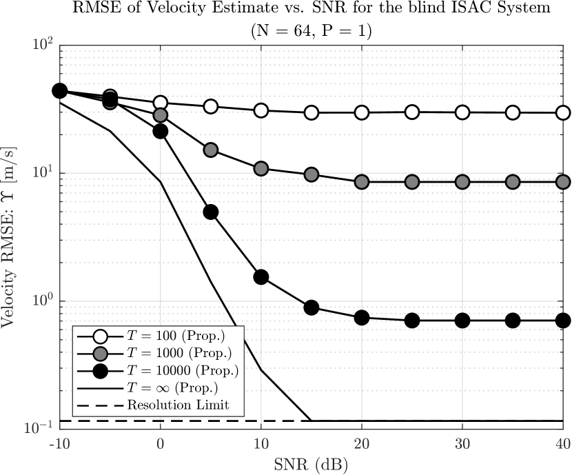
Figure 3: Velocity RMSE versus SNR performance of the proposed blind bistatic RPE scheme over the AFDM waveform with a single LoS signal from the active (static) BS and one NLoS echo signal from a target in the surrounding.

We remark here that since a LoS path always exists in the surrounding defining the active BS, there will always be more that one target to be detected by the estimation algorithm, which concurrently fits with the positive semidefinite constraint in use in the final optimization problem.

The remaining system parameters for the results shown in Figures 2 and 3 are as follows: $70\,\text{GHz}$ central carrier frequency, with a bandwidth of $20\,\text{MHz}$, quadrature amplitude modulation (QAM) modulation and maximum normalized delay and digital Doppler shift indices $\ell_{\text{max}}=4$ and $f_{\text{max}}=0.1$, respectively. In order to reduce complexity, we also set $N=64$ for AFDM.

Consequently, the proposed blind RPE algorithm employs the optimization hyperparameters $\beta=1$, $\eta=0.1$, $\alpha=0.001$ and is run up to $i_{\text{max}}=3$ iterations.

As seen from Figures 2 and 3, the RMSE performance increases significantly when an increasing amount of received frames are utilized during the construction of the sample covariance matrix, with the case for an infinite number of transmit frames converging with the resolution limit [31] obtained when the true $\bar{\mathbf{H}}_{\mathrm{G}}$ is estimated under AFDM waveforms. However, due to the constraints that were dropped from the original optimization problem given in equation (34), there is an error floor for the resulting estimation which will be addressed in a follow-up journal version of this article.

V Conclusion

In this paper, we contributed a new CC-ISAC scheme, namely, a blind bistatic RPE technique for any arbitrary communications waveform. This was achieved by formulating a novel covariance-based problem, then solved completely by introducing an arbitrarily-tight approximation for the $\ell_{0}$-norm term in the optimization problem via FP. Finally, we proved the efficacy of the the proposed method with computer simulations, which demonstrated the performance by the way of the RMSE for both range and velocity.

References

- [1] T. Wild, V. Braun, and H. Viswanathan, “Joint Design of Communication and Sensing for Beyond 5G and 6G Systems,” IEEE Access, vol. 9, pp. 30 845–30 857, 2021.
- [2] C.-X. Wang, X. You, X. Gao, X. Zhu, Z. Li, C. Zhang, H. Wang, Y. Huang, Y. Chen, H. Haas, J. S. Thompson, E. G. Larsson, M. D. Renzo, W. Tong, P. Zhu, X. Shen, H. V. Poor, and L. Hanzo, “On the Road to 6G: Visions, Requirements, Key Technologies, and Testbeds,” IEEE Communications Surveys & Tutorials, vol. 25, no. 2, pp. 905–974, 2023.
- [3] N. González-Prelcic, M. F. Keskin, O. Kaltiokallio, M. Valkama, D. Dardari, X. Shen, Y. Shen, M. Bayraktar, and H. Wymeersch, “The Integrated Sensing and Communication Revolution for 6G: Vision, Techniques, and Applications,” Proceedings of the IEEE, pp. 1–0, 2024.
- [4] S. D. Liyanaarachchi, T. Riihonen, C. B. Barneto, and M. Valkama, “Optimized Waveforms for 5G–6G Communication with Sensing: Theory, Simulations and Experiments,” IEEE Transactions on Wireless Communications, vol. 20, no. 12, pp. 8301–8315, 2021.
- [5] S. K. Mohammed, R. Hadani, A. Chockalingam, and R. Calderbank, “OTFS—A Mathematical Foundation for Communication and Radar Sensing in the Delay-Doppler Domain,” IEEE BITS the Information Theory Magazine, vol. 2, no. 2, pp. 36–55, 2022.
- [6] Z. Gao, Z. Wan, D. Zheng, S. Tan, C. Masouros, D. W. K. Ng, and S. Chen, “Integrated Sensing and Communication with mmWave Massive MIMO: A Compressed Sampling Perspective,” IEEE Transactions on Wireless Communications, vol. 22, no. 3, pp. 1745–1762, 2023.
- [7] W. Zhou, R. Zhang, G. Chen, and W. Wu, “Integrated Sensing and Communication Waveform Design: A Survey,” IEEE Open Journal of the Communications Society, vol. 3, pp. 1930–1949, 2022.
- [8] H. S. Rou, G. T. F. de Abreu, J. Choi, D. G. G., M. Kountouris, Y. L. Guan, and O. Gonsa, “From OTFS to AFDM: A Comparative Study of Next-Generation Waveforms for ISAC in Doubly-Dispersive Channels,” https://arxiv.org/abs/2401.07700, 2024.
- [9] C. Baquero Barneto, T. Riihonen, M. Turunen, L. Anttila, M. Fleischer, K. Stadius, J. Ryynänen, and M. Valkama, “Full-Duplex OFDM Radar with LTE and 5G NR Waveforms: Challenges, Solutions, and Measurements,” IEEE Transactions on Microwave Theory and Techniques, vol. 67, no. 10, pp. 4042–4054, 2019.
- [10] L. Gaudio, M. Kobayashi, G. Caire, and G. Colavolpe, “On the Effectiveness of OTFS for Joint Radar Parameter Estimation and Communication,” IEEE Transactions on Wireless Communications, vol. 19, no. 9, pp. 5951–5965, 2020.
- [11] A. Bemani, N. Ksairi, and M. Kountouris, “Integrated Sensing and Communications with Affine Frequency Division Multiplexing,” IEEE Wireless Communications Letters, pp. 1–1, 2024.
- [12] ——, “AFDM: A Full Diversity Next Generation Waveform for High Mobility Communications,” in IEEE International Conference on Communications Workshops (ICC Workshops), 2021, pp. 1–6.
- [13] ——, “Affine Frequency Division Multiplexing for Next Generation Wireless Communications,” IEEE Transactions on Wireless Communications, vol. 22, no. 11, pp. 8214–8229, 2023.
- [14] S. Khaledian, F. Farzami, B. Smida, and D. Erricolo, “Inherent Self-Interference Cancellation for In-Band Full-Duplex Single-Antenna Systems,” IEEE Transactions on Microwave Theory and Techniques, vol. 66, no. 6, pp. 2842–2850, 2018.
- [15] J. A. Zhang, Y. J. Guo, and K. Wu, Joint Communications and Sensing: From Fundamentals to Advanced Techniques. Wiley-IEEE Press, 2023.
- [16] H. Kuschel, D. Cristallini, and K. E. Olsen, “Tutorial: Passive Radar Tutorial,” IEEE Aerospace and Electronic Systems Magazine, vol. 34, no. 2, pp. 2–19, 2019.
- [17] M. Malanowski, Signal Processing for Passive Bistatic Radar. Artech, 2006.
- [18] H. Griffiths and C. Baker, An Introduction to Passive Radar, Second Edition. Artech, 2022.
- [19] L. Leyva, D. Castanheira, A. Silva, and A. Gameiro, “Two-stage estimation algorithm based on interleaved OFDM for a cooperative bistatic ISAC scenario,” in 2022 IEEE 95th Vehicular Technology Conference: (VTC2022-Spring), 2022, pp. 1–6.
- [20] J. Zhu, Y. Tang, F. Liu, X. Zhang, H. Yin, and Y. Zhou, “AFDM-Based Bistatic Integrated Sensing and Communication in Static Scatterer Environments,” IEEE Wireless Communications Letters, pp. 1–1, 2024.
- [21] D. W. Bliss and S. Govindasamy, Dispersive and doubly dispersive channels. Cambridge University Press, 2013, pp. 341–364.
- [22] K. R. R. Ranasinghe, H. S. Rou, G. T. F. de Abreu, T. Takahashi, and K. Ito, “Joint Channel, Data and Radar Parameter Estimation for AFDM Systems in Doubly-Dispersive Channels,” https://arxiv.org/pdf/2405.16945, 2024.
- [23] J. Zhu, Y. Tang, X. Wei, H. Yin, J. Du, Z. Wang, and Y. Liu, “A low-complexity radar system based on affine frequency division multiplexing modulation,” arXiv preprint arXiv:2312.11125, 2023.
- [24] H. S. Rou, K. Yukiyoshi, T. Mikuriya, G. T. F. de Abreu, and N. Ishikawa, “AFDM Chirp-Permutation-Index Modulation with Quantum-Accelerated Codebook Design,” arXiv preprint arXiv:2405.02085, 2024.
- [25] O. K. Rasheed, G. D. Surabhi, and A. Chockalingam, “Sparse delay-doppler channel estimation in rapidly time-varying channels for multiuser otfs on the uplink,” in 2020 IEEE 91st Vehicular Technology Conference (VTC2020-Spring), 2020, pp. 1–5.
- [26] A. Mehrotra, S. Srivastava, A. K. Jagannatham, and L. Hanzo, “Data-Aided CSI Estimation Using Affine-Precoded Superimposed Pilots in Orthogonal Time Frequency Space Modulated MIMO Systems,” IEEE Transactions on Communications, vol. 71, no. 8, pp. 4482–4498, 2023.
- [27] J. Tropp, “Just relax: convex programming methods for identifying sparse signals in noise,” IEEE Transactions on Information Theory, vol. 52, no. 3, pp. 1030–1051, 2006.
- [28] P. Cao, J. Thompson, and H. V. Poor, “A sequential constraint relaxation algorithm for rank-one constrained problems,” in 2017 25th European Signal Processing Conference (EUSIPCO), 2017, pp. 1060–1064.
- [29] H. Iimori, G. T. F. De Abreu, T. Hara, K. Ishibashi, R.-A. Stoica, D. González G., and O. Gonsa, “Robust Symbol Detection in Large-Scale Overloaded NOMA Systems,” IEEE Open Journal of the Communications Society, vol. 2, pp. 512–533, 2021.
- [30] K. Shen and W. Yu, “Fractional Programming for Communication Systems—Part I: Power Control and Beamforming,” IEEE Transactions on Signal Processing, vol. 66, no. 10, pp. 2616–2630, 2018.
- [31] K. R. R. Ranasinghe, H. S. Rou, and G. T. F. de Abreu, “Fast and Efficient Sequential Radar Parameter Estimation in MIMO-OTFS Systems,” in ICASSP 2024 - 2024 IEEE International Conference on Acoustics, Speech and Signal Processing (ICASSP), 2024, pp. 8661–8665.