Thermodynamic topology of topological charged dilatonic black holes

Abstract

The aim of this paper is to explore the thermodynamic topology of topological charged dilatonic black holes. To achieve this, our study will begin by examining the characteristics of topological charged black holes in dilaton gravity. Specifically, we will concentrate on the impact of the topological constant on the event horizon of these black holes. Subsequently, we will analyze these black holes, considering their thermodynamic and conserved quantities, in order to assess the validity of the first law of thermodynamics. We explore the thermodynamic topology of these black holes by treating them as thermodynamic defects. For our study, we examine two types of thermodynamic ensembles: the fixed $q$ ensemble and the fixed $\phi$ ensemble. To study the impact of the topological constant ($k$) on thermodynamic topology, we consider all possible types of curvature hypersurfaces that can form in these black holes. By calculating the topological charges at the defects within their thermodynamic spaces, we analyze both the local and global topology of these black holes. We also investigate how the parameters of dilaton gravity affect the thermodynamic topology of black holes and highlight the differences compared to charged black holes in the General Relativity.

I Introduction

Despite many successes in agreement with observations, General Relativity (GR) cannot explain some phenomena such as the cosmological constant problem [1], the origin of acceleration of our universe [2, 3], cosmic microwave background (CMB) radiation [4, 5], and the existence of dark energy and dark matter. So we need to modify this theory of gravity. On the other hand, dark energy and especially dark matter have received much attention recently. In theoretical physics, non-baryonic dark matter has been classified into three models: cold, warm, and hot [6]. The dilaton field is one of the most fascinating candidates for cold dark matter because the cold dark matter model agrees well with experimental observations [7]. In addition, considering a new scalar field is one of the best ways to find the nature of dark energy [8, 9]. It is notable that, the low energy limit of string theory contains a dilaton field that is coupled to gravity. The dilaton coupling with other gauge fields profoundly affects the resulting solutions [10, 11, 12, 13, 14, 15]. For example, it was indicated that a dilaton field can change the asymptotic behavior of the spacetime. In particular, in the presence of one or two Liouville-type dilaton potentials, black hole spacetimes are neither asymptotically flat nor (anti)-de Sitter ((A)dS) [16, 17, 18, 19, 20]. This is because the dilaton field does not vanish for $r\rightarrow\infty$. Furthermore, it was shown that the combination of three Liouville-type dilaton potentials allows the construction of dilaton black hole solutions on the (A)dS spacetime background [21, 22]. It was also shown that the dilaton charges are expressed as black hole masses and the scalar dilaton field acts as a secondary hair. Furthermore, the dilaton field could change the causal structure of the black hole and lead to the curvature singularities at finite radii [16, 17, 18, 19]. Therefore, adding a dilaton field to GR to investigate the physical properties of black holes has been getting more attention [23, 24, 25, 26, 27, 28, 29, 30, 31, 32, 33, 34, 35, 36, 37, 38, 39, 40].

From a quantum perspective, black holes are capable of emitting energy, a phenomenon known as Hawking radiation. This leads us to consider black holes as thermal objects with a specific temperature [41, 42]. Furthermore, black holes possess a measurable entropy, referred to as the Hawking-Bekenstein entropy, which can be derived from their surface area [43, 44]. Building upon these concepts, Bardeen et al. introduced the thermodynamics of black holes [45]. In this regard, researchers have dedicated numerous years to studying the thermodynamics of various types of black holes. Some investigations have focused on the extended phase space using the anti-de Sitter/Conformal Field Theory (AdS/CFT) correspondence [46, 47]. In this approach, the cosmological constant is treated as pressure [48], offering valuable insights into black hole phase transitions [49, 50, 51, 52, 53, 54, 55, 56, 57, 58, 59].

The study of black hole thermodynamics has generated significant interest in the field of topology. Two topological approaches have been developed to investigate the thermodynamic properties of various black hole systems. A topological concept was introduced in Ref. [60], which involves a vector with zero points that correspond to the critical point. According to Duan’s pioneering $\phi$-mapping topological current theory [61, 62], these zero points represent defects of the vector, as the direction of the vector is undefined at these points. From a topological standpoint, each defect can be assigned a winding number, which is an integer value. By summing all the winding numbers, a topological number is obtained, allowing for the classification of the systems into different topological classes. Within each class, the systems share similar thermodynamic properties. Specifically, based on the value of the winding number, the critical point is divided into two classes: the conventional class and the novel class. These classes exhibit opposite properties in terms of the generation and annihilation of the black hole branches. Furthermore, the black hole systems are grouped into different classes based on the structures of the critical points. In this regard, the thermodynamic topology of black holes has been studied by considering various black holes in much literature [63, 64, 65, 66, 67, 68, 69, 70, 71, 72, 73, 74, 75, 76, 77, 78, 79, 80, 81]. In this paper, we follow the topological approach proposed in Ref. [64], and study the thermodynamic topology by treating the charged dilatonic black holes as topological defects.

This paper is organized as follows. In Section II, we derive the solution for topological charged black holes in dilaton gravity. Section III discusses the thermodynamic properties and conserved quantities associated with this solution. Section IV explores the concept of thermodynamic topology and outlines the mathematical procedures needed for its investigation. Subsections IV.1 and IV.2 focus on two statistical ensembles: the fixed charge ($q$) ensemble and the fixed potential ($\phi$) ensemble. Within these subsections, we examine various types of curvature hypersurfaces to understand how the topological constant ($k$) impacts thermodynamic topology. Finally, section V provides our conclusions and closing remarks on the study.

II Black hole solution

The action of charged dilaton gravity is [82]

$$\mathcal{I}=\frac{1}{16\pi}\int d^{4}x\sqrt{-g}\left[\mathcal{R}-2\left(\nabla\Phi\right)^{2}-V\left(\Phi\right)-e^{-2\alpha\Phi}F_{\mu\nu}F^{\mu\nu}\right],$$ (1)

in the above action, $\mathcal{R}$ represents the Ricci scalar curvature, $\Phi$ represents the dilaton field, and $V\left(\Phi\right)$ represents the potential for $\Phi$. The electromagnetic field is denoted by $F_{\mu\nu}=\partial_{\mu}A_{\nu}-\partial_{\nu}A_{\mu}$, with $A_{\mu}$ representing the electromagnetic potential. It is important to note that $\alpha$ is a constant that determines the strength of the coupling between the scalar and electromagnetic fields. For our purposes of finding a black hole with a radial electric field ($F_{tr}(r)=-F_{rt}(r)\neq 0$), the form of the electromagnetic potential will be as follows

$$A_{\mu}=\delta_{\mu}^{0}h\left(r\right).$$ (2)

By utilizing the variational principle and by varying Eq. (1) with respect to the gravitational field $g_{\mu\nu}$, the dilaton field $\Phi$, and the gauge field $A_{\mu}$, we are able to obtain the subsequent field equations [82].

$$R_{\mu\nu} = 2\left(\partial_{\mu}\Phi\partial_{\nu}\Phi+\frac{1}{4}g_{\mu\nu}V(\Phi)\right)+2e^{-2\alpha\Phi}\left(F_{\mu\eta}F_{\nu}^{\eta}-\frac{1}{4}g_{\mu\nu}F_{\lambda\eta}F^{\lambda\eta}\right),$$ (3)

$$\nabla^{2}\Phi = \frac{1}{4}\frac{\partial V}{\partial\Phi}-\frac{\alpha}{2}e^{-2\alpha\Phi}F_{\lambda\eta}F^{\lambda\eta},$$ (4)

$$\nabla_{\mu}\left(e^{-2\alpha\Phi}F^{\mu\nu}\right) = 0.$$ (5)

The objective of this paper is to obtain topological charged black hole solutions from Einstein-Maxwell-dilaton gravity. To accomplish this, we will employ the following static metric ansatz

$$ds^{2}=-f(r)dt^{2}+\frac{dr^{2}}{f(r)}+r^{2}R^{2}(r)d\Omega_{k}^{2},$$ (6)

where the functions $f(r)$ and $R(r)$ must be determined, while $d\Omega_{k}^{2}$ represents the line element of a $2-$dimensional hypersurface with a constant curvature of $2k$ and volume $\mathcal{V}$. It is important to note that the constant $k$ indicates that the boundary of $t=constant$ and $r=constant$ can be a positive (elliptic), zero (flat), or negative (hyperbolic) constant curvature hypersurface, expressed explicitly as follows

$$d\Omega_{k}^{2}=\left\{\begin{array}[]{cc}d\theta^{2}+\sin^{2}\theta d\varphi^{2},&k=1\\ d\theta^{2}+\sinh^{2}\theta d\varphi^{2},&k=-1\\ d\theta^{2}+d\varphi^{2},&k=0\end{array}\right..$$ (7)

by utilizing Eqs. (2), (5) and (6), it is possible to derive the electromagnetic tensor

$$F_{tr}=\frac{qe^{2\alpha\Phi\left(r\right)}}{r^{2}R^{2}(r)},$$ (8)

where $q$ is an integration constant that is associated with the electric charge of the black hole.

Here, we employ an adjusted form of a Liouville-type dilation potential to discover metric functions that are consistent. The modified version of the potential has the following form [28]

$$V(\Phi)=\frac{2k\alpha^{2}}{b^{2}\mathcal{K}_{1,-1}}e^{\frac{2\Phi\left(r\right)}{\alpha}}+2\Lambda e^{2\alpha\Phi\left(r\right)},$$ (9)

where $\Lambda$ is a free parameter which plays the role of the cosmological constant. Also, we define $\mathcal{K}_{ij}$ as $\mathcal{K}_{i,j}=i\alpha^{2}+j$, for example, $\mathcal{K}_{1,-1}=\alpha^{2}-1$. It is notable that, the Liouville-type dilation potential, denoted as $V(\Phi)$, is utilized in the study of Einstein-Maxwell-dilaton black holes [25], and Friedman-Robertson-Walker scalar field cosmologies [83].

Next, by applying the ansatz $R(r)=e^{\alpha\Phi(r)}$ and substituting Eq. (8) into the field equations (Eqs. (3) and (4)), we can obtain the following solutions in Einstein-Maxwell-dilaton gravity [84, 85]

$$f(r) = -\frac{\mathcal{K}_{1,1}}{\mathcal{K}_{1,-1}}k\left(\frac{b}{r}\right)^{\frac{-2\alpha^{2}}{\mathcal{K}_{1,1}}}-\frac{m}{r^{\frac{\mathcal{K}_{-1,1}}{\mathcal{K}_{1,1}}}}+\frac{\mathcal{K}_{1,-1}^{2}\Lambda r^{2}}{\mathcal{K}_{1,-3}}\left(\frac{b}{r}\right)^{\frac{2\alpha^{2}}{\mathcal{K}_{1,1}}}+\frac{q^{2}\mathcal{K}_{1,1}}{r^{2}}\left(\frac{b}{r}\right)^{\frac{-2\alpha^{2}}{\mathcal{K}_{1,1}}},$$ (10)

$$\Phi(r) = \frac{\alpha}{\mathcal{K}_{1,1}}\ln\left(\frac{b}{r}\right),$$ (11)

where $b$ is an arbitrary constant. Additionally, in the above expression, $m$ is an integration constant that is associated with the geometrical mass of the black hole. It is worth noting that when the parameters of dilaton gravity, i.e. $\alpha=0$, are absent, the solution (10) becomes a $4$-dimensional asymptotically AdS topological charged black hole in GR with a positive, zero, or negative constant curvature hypersurface, as

$$f(r)=k-\frac{m}{r}-\frac{\Lambda}{3}r^{2}+\frac{q^{2}}{r^{2}}.$$ (12)

We are searching for the curvature singularity to validate the interpretation of the solutions as black holes. Therefore, we calculate the Kretschmann scalar. The calculations indicate that the Kretschmann scalar is finite for finite values of the radial coordinates. However, for extremely small and large values of $r$, we obtain the following results

$$\lim_{r\rightarrow 0}R_{\alpha\beta\mu\nu}R^{\alpha\beta\mu\nu} \propto r^{-\frac{4\mathcal{K}_{1,2}}{\mathcal{K}_{1,1}}},$$ (13)

$$\lim_{r\rightarrow\infty}R_{\alpha\beta\mu\nu}R^{\alpha\beta\mu\nu} = \frac{12(\alpha^{4}-2\alpha^{2}+2)\Lambda}{\mathcal{K}_{-1,3}^{2}}\left(\frac{b}{r}\right)^{\frac{4\alpha^{2}}{\mathcal{K}_{1,1}}},$$ (14)

Equation (13) confirms the presence of an essential singularity at $r=0$, while Eq. (14) demonstrates that, for nonzero $\alpha$, the solutions do not exhibit asymptotically flat or (A)dS behavior.

Here, we plot the metric function $f(r)$ versus $r$ in Figs. 1 and 2 to demonstrate that the singularity at $r=0$ is indeed concealed by an event horizon. Additionally, this visualization allows us to observe the impact of dilaton gravity and the constant $k$ on the event horizon.

The effect of the constant $k$ on the root of the metric function is illustrated in Fig. 1. It is evident from the figure that there are two roots. It is important to note that the outer root is associated with the event horizon. Furthermore, our findings suggest that the larger black holes correspond to $k=-1$, $k=0$, and $k=+1$, respectively, meaning that $r_{{+}_{k=-1}}>r_{{+}_{k=0}}>r_{{+}_{k=+1}}$ (where $r_{{+}_{k}}$ represents the event horizon for different values of $k$).

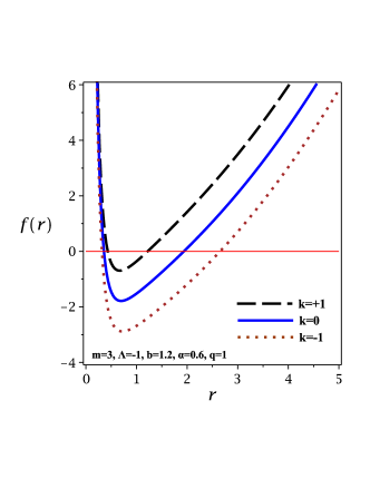
Figure 1: $f(r)$ versus $r$ for different values of $k$.

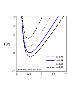
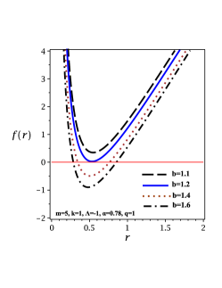
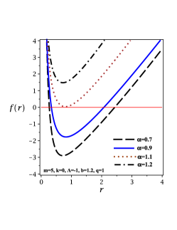
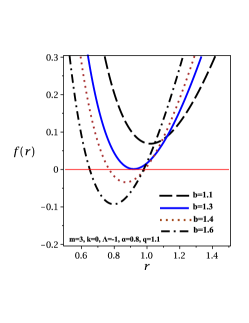
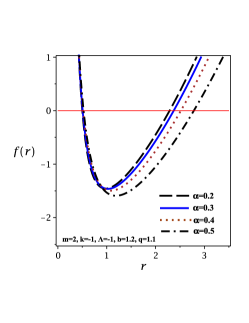
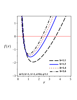
Figure 2: $f(r)$ versus $r$ for different values of $k$, $\alpha$, and $b$. The up panels are for $k=+1$. The middle panels are for $k=0$. The down panels are for $k=-1$.

Now, we are studying the effects of dilaton gravity ($\alpha$ and $b$) on the event horizon of black holes for different values of $k$. Our findings indicate the following:

1) The metric function ($f(r)$) plotted against $r$ for $k=1$ is shown in the up panels of Fig. 2. The results show that as we increase $\alpha$, the root of the metric function decreases, and eventually there is no root for the metric function (up left panel in Fig. 2). In other words, increasing $\alpha$ leads to the existence of a naked singularity. However, there is a different behavior for $b$. In fact, as we increase $b$, the root of the metric function increases, and we encounter large black holes when $b$ is large.

2) For $k=0$, the middle panels of Fig. 2 show the plot of $f(r)$. Similar to the previous case, the roots of the metric function increase (decrease) as $b$ ($\alpha$) increases (decreases). Therefore, when we consider small and large values of $\alpha$ and $b$ respectively, we find large charged dilatonic black holes.

3) The metric function ($f(r)$) plotted against $r$ for $k=-1$ is shown in the down panels of Fig. 2. The results reveal that the behavior of the root of the metric function is opposite to that of the two previous cases. Indeed, for $k=-1$, large black holes have large values of $\alpha$ and small values of $b$.

III Thermodynamical Quantities

Now, we can calculate the thermodynamic and conserved quantities of the obtained solutions and determine whether these quantities satisfy the first law of thermodynamics.

To analyze temperature, we employ the concept of surface gravity. The temperature of these solutions is obtained as follows [84, 85]

$$T=\frac{\mathcal{K}_{1,1}\left(\frac{b}{r_{+}}\right)^{\frac{-2\alpha^{2}}{\mathcal{K}_{1,1}}}}{4\pi}\left[\frac{k}{\mathcal{K}_{-1,1}r_{+}}-\frac{q^{2}}{r_{+}^{3}}-\Lambda r_{+}\left(\frac{b}{r_{+}}\right)^{\frac{4\alpha^{2}}{\mathcal{K}_{1,1}}}\right],$$ (15)

where $r_{+}$ is related to the event horizon and satisfies $f(r=r_{+})=0$.

The entropy of a black hole is determined using the area law. For these black holes we get

$$S=\frac{\widetilde{S}}{\mathcal{V}}=\frac{r_{+}^{2}}{4}\left(\frac{b}{r_{+}}\right)^{\frac{2\alpha^{2}}{\mathcal{K}_{1,1}}},$$ (16)

in which by setting $\alpha=0$, the entropy of dilatonic black holes reduces to the entropy of black holes in Einstein-Maxwell’s theory.

To determine the total electric charge of the solutions, Gauss’s law can be utilized. By calculating the flux of the electric field, we can determine the total electric charge which is [84, 85]

$$Q=\frac{\widetilde{Q}}{\mathcal{V}}=\frac{q}{4\pi}.$$ (17)

Next, our goal is to calculate the electric potential. We can achieve this by analyzing the equation $F_{\mu\nu}=\partial{\mu}A{\nu}-\partial{\nu}A{\mu}$. By doing so, we can identify the non-zero component of the gauge potential, which is denoted as $A_{t}=-\int{F_{tr}dr}$. Consequently, we can determine the electric potential at the event horizon ($U$) in relation to the reference point ($r\rightarrow\infty$) as follows

$$U\left(r\right)=-\int_{r_{+}}^{+\infty}F_{tr}dr=\frac{q}{r_{+}}.$$ (18)

Finally, the total mass of the solution is determined based on the definition of mass provided by Abbott and Deser [86, 87, 88] (see Refs. [84, 85], for more details)

$$M=\frac{\widetilde{M}}{\mathcal{V}}=\frac{A}{8\pi\mathcal{K}_{-1,1}},$$ (19)

where

$$A=\left(\frac{b}{r_{+}}\right)^{\frac{4\alpha^{2}}{\mathcal{K}_{1,1}}}\left[kr_{+}-\frac{q^{2}\mathcal{K}_{1,-1}}{r_{+}}+\frac{\mathcal{K}_{1,1}\mathcal{K}_{-1,1}\Lambda r_{+}^{3}\left(\frac{b}{r_{+}}\right)^{\frac{4\alpha^{2}}{\mathcal{K}_{1,1}}}}{\mathcal{K}_{1,-3}}\right].$$ (20)

It is worth mentioning that when $\alpha=0$, Eq. (19) simplifies to the mass of the Einstein-Maxwell black holes [84].

To determine if the quantities obtained, temperature (Eq. (15)), entropy (Eq. (16)), electric charge (Eq. (17)), electric potential (Eq. (18)), and total mass of black holes (Eq. (19), satisfy the first law of thermodynamics, we show that

$$\left(\frac{\partial M}{\partial S}\right)_{Q}=T\text{ \ \ \ \ }\&\text{\ \ \ \ \ }\left(\frac{\partial M}{\partial Q}\right)_{S}=U,$$ (21)

so, these quantities be able to satisfy the first law of thermodynamics, which is

$$dM=\left(\frac{\partial M}{\partial S}\right)_{Q}dS+\left(\frac{\partial M}{\partial Q}\right)_{S}dQ.$$ (22)

IV Thermodynamic Topology

To explore thermodynamic topology, we employ the off-shell free energy method, which views black hole solutions as topological defects within their thermodynamic context. This approach involves analyzing both local and global topology by calculating winding numbers associated with these defects. These winding numbers categorize black holes based on their overall topological charge. Importantly, a black hole’s thermal stability correlates with the sign of its winding number. The fundamental idea behind thermodynamic topology revolves around understanding these topological defects and their associated charges. Below, we discuss the essential mathematical procedures involved in investigating thermodynamic topology.

In black hole thermodynamics, a vector field is derived from the generalized off-shell free energy. The expression for the off-shell free energy of a black hole with arbitrary mass, given by [64]

$$\mathcal{F}=E-\frac{S}{\tau},$$ (23)

where $E$ represents the energy (equivalent to the mass $M$) and $S$ denotes the entropy of the black hole. The parameter $\tau$, representing the timescale, is allowed to vary freely. To leverage this generalized free energy, a vector field $\phi$ is defined as [64]

$$\phi=\left(\phi^{r},\phi^{\Theta}\right)=\left(\frac{\partial\mathcal{F}}{\partial r_{+}},-\cot\Theta~{}\csc\Theta\right).$$ (24)

The zero points of this vector field are always obtained to be $(\tau,\Theta)=(\frac{1}{T},\frac{\pi}{2})$ where $T$ is the equilibrium temperature of the cavity that encloses the black hole (on shell temperature). At the points where a vector field either diverges or is not defined, these locations carry significant physical implications. Specifically, in our context, these points correspond to the zero points or defects of the vector field, which represent black hole solutions. In essence, we can interpret black holes as topological defects of the constructed vector field. Consequently, each black hole solution possesses a topological charge. We use Duan’s $\phi$ mapping technique to determine the associated topological charge. We calculate the unit vector $n$ of the field in Eq. (24), which are

$$n^{1} = \frac{\phi^{r}}{\sqrt{(\phi^{r})^{2}+(\phi^{\Theta})^{2}}},$$

$$n^{2} = \frac{\phi^{\Theta}}{\sqrt{(\phi^{r})^{2}+(\phi^{\Theta})^{2}}},$$

The vector $n^{a}$ must satisfy two key conditions

$$n^{a}n^{a}=1\quad\text{and}\quad n^{a}\partial_{\nu}n^{a}=0,$$

where $\partial_{\nu}=\frac{\partial}{\partial x^{\nu}}$ and $\mu,\nu,\rho=0,1,2$.

We construct a topological current $j^{\mu}$ in the coordinate space $x^{\nu}=\{t,r_{+},\theta\}$ defined by

$$j^{\mu}=\frac{1}{2\pi}\epsilon^{\mu\nu\rho}\epsilon_{ab}\partial_{\nu}n^{a}\partial_{\rho}n^{b},$$ (26)

the current $j^{\mu}$ is conserved, meaning

$$\partial_{\mu}j^{\mu}=0.$$ (27)

The current in equation (26) can be written as

$$j^{\mu}=\delta^{2}(\phi)J^{\mu}\left(\frac{\phi}{x}\right),$$ (28)

where $J^{\mu}$ relates to the Jacobi tensor $\epsilon^{ab}J^{\mu}\left(\frac{\phi}{x}\right)=\epsilon^{\mu\nu\rho}\partial_{\nu}\phi^{a}\partial_{\rho}\phi^{b}$. We use the Laplacian Green function $\triangle_{\phi^{a}}ln||\phi||=2\pi\delta^{2}(\phi)$ to get the equation (28).

The topological charge $W$ relates to the zeroth component of the current density as

$$W=\int_{\Sigma}j^{0}d^{2}x=\sum_{i=1}^{N}w_{i},$$ (29)

where $w_{i}$ denotes the winding number around each zero point of the vector field $\phi$. $\Sigma$ is the parameter region in which we calculate the winding number $w_{i}$. Contours with appropriate dimensions are constructed to define the parameter region, as follows

$$\begin{cases}r_{+}=r_{1}\cos\nu+r_{0},\\ \\ \theta=r_{2}\sin\nu+\frac{\pi}{2},\end{cases}$$ (30)

where $\nu\in(0,2\pi)$. Also, $r_{1}$ and $r_{2}$ are parameters that define the dimensions of the contour to be formed and $r_{0}$ represents the center point around which the contour is created. The winding numbers $w_{i}$ quantify how the vector field $n$ deflects along contours enclosing each zero point. The mathematical relation between deflection angle $\Omega$ and winding number is given by

$$w_{i}=\frac{\Omega(2\pi)}{2\pi},$$ (31)

where $\Omega$ is obtained by employing the following contour integration

$$\Omega(\nu)=\int_{0}^{\nu}\epsilon_{12}n^{1}\partial_{\nu}n^{2}d\nu.$$ (32)

From Eq. (31), the topological charge is calculated by taking the sum of the winding numbers calculated around all zero points of the vector field $\phi$ or $W=\sum_{i=1}w_{i}$. This topological charge $W$ provides insight into the structural properties of black hole solutions within the framework of thermodynamic topology. It is important to highlight that $j^{\mu}$ is only non-zero at the zero points of the vector field $\phi$. Thus, the total topological charge is considered zero if there are no zero points within the parameter region.

In the next two subsections, we explore the thermodynamic topology of topological charged dilatonic black holes. Our study focuses on two types of thermodynamic setups: one where the charge ($q$) is fixed, and another where the potential ($\phi$) is fixed. By calculating the topological properties of these thermodynamic entities, we analyze both the local and global structure of these black holes. We investigate how the topological constant ($k$) influences the thermodynamic characteristics. Additionally, we examine how the parameters of dilaton gravity impact the thermodynamic characteristics of these black holes, emphasizing differences from charged black holes described by GR.

IV.1 Fixed charge ($q$) ensemble

IV.1.1 For elliptic ($k=1$) curvature hypersurface

In fixed charge ensemble, charge $q$ is a constant quantity. The off-shell free energy is calculated using equations (16) and (19), which leads to

$$\mathcal{F}=M-\frac{S}{\tau}=\frac{\left(\frac{b}{r_{+}}\right){}^{\frac{4\alpha^{2}}{\mathcal{K}_{1,1}}}\left(\frac{\mathcal{K}_{1,1}\Lambda r_{+}^{4}\left(\frac{b}{r_{+}}\right){}^{\frac{4\alpha^{2}}{\mathcal{K}_{1,1}}}}{\mathcal{K}_{1,-3}}-\frac{kr_{+}^{2}}{\mathcal{K}_{1,-1}}+q^{2}\right)}{8\pi r_{+}}-\frac{r_{+}^{2}}{4\tau}\left(\frac{b}{r_{+}}\right){}^{\frac{2\alpha^{2}}{\mathcal{K}_{1,1}}}.$$ (33)

Taking the first order derivative of the off-shell free energy, the $\phi^{r}$ component is found to be

$$\phi^{r}=\frac{\left(\frac{b}{r_{+}}\right)^{\frac{4\alpha^{2}}{\mathcal{K}_{1,1}}}}{8\pi\mathcal{K}_{1,1}r_{+}^{2}}\left(\frac{\mathcal{K}_{3,-1}kr_{+}^{2}}{\mathcal{K}_{1,-1}}-\frac{\mathcal{K}_{1,1}\mathcal{K}_{5,-3}\Lambda r_{+}^{4}\left(\frac{b}{r_{+}}\right)^{\frac{4\alpha^{2}}{\mathcal{K}_{1,1}}}}{\mathcal{K}_{1,-3}}-\frac{4\pi r_{+}^{3}}{\tau\left(\frac{b}{r_{+}}\right)^{\frac{2\alpha^{2}}{\mathcal{K}_{1,1}}}}-q^{2}\mathcal{K}_{5,1}\right).$$ (34)

Solving $\phi^{r}=0$, $\tau$ can be obtained in the following form

$$\tau=\frac{4\pi r_{+}^{3}\left(\frac{b}{r_{+}}\right)^{\frac{-2\alpha^{2}}{\mathcal{K}_{1,1}}}}{\frac{\mathcal{K}_{3,-1}kr_{+}^{2}}{\mathcal{K}_{1,-1}}-\frac{\mathcal{K}_{1,1}\mathcal{K}_{5,-3}\Lambda r_{+}^{4}\left(\frac{b}{r_{+}}\right){}^{\frac{4\alpha^{2}}{\mathcal{K}_{1,1}}}}{\mathcal{K}_{1,-3}}-q^{2}\mathcal{K}_{5,1}}.$$ (35)

(a)

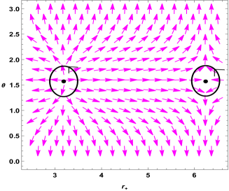
(b)

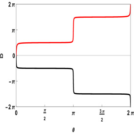
(c)

Figure 3: Topological charge of topological charged dilatonic black holes $(k=1)$ in fixed charge ensemble when positive values of $\Lambda$ is considered. Here we have considered $q=1$, $\alpha=0.5$, $b=1$, $k=1$, $\Lambda=0.01$.

Next, $\tau$ vs $r_{+}$ is plotted in Fig. 3(a) for $q=1$, $\alpha=0.5$, $b=1$, $\Lambda=0.01$ and $k=1$. This plot reveals two black hole branches: a small black hole branch for the range $r_{+}<4.0867$ and a large black hole branch for $r_{+}>4.0867$. To calculate topological charge of the black hole we choose a random value of $\tau=\tau_{1}=800$ and calculate the zero point of the vector field. In Fig. 3(b), the vectors represent a part of the ($n^{1}$,$~{}n^{2}$) field in the $r_{+}-\theta$ plane, where the zero points for $\tau=\tau_{1}=800$ are observed at $r_{+}=3.1842$ and $r_{+}=6.24193$. The topological charge is calculated in Fig. 3(c), where the winding number corresponding to $r_{+}=3.1842$ is $+1$ represented by the red solid line and the winding number corresponding to $r_{+}=6.24193$ is $-1$, represented by the black solid line. By adding the winding number the topological charge $W$ is obtained as $W=1-1=0.$
We solve the equation $\frac{\partial\tau}{\partial r_{+}}=0$ to obtain the exact point at which the phase transition takes place i.e., $(\tau_{c}$, $r_{c})=(579.841$, $4.0867)$ represented by the blue dot in Fig. 3(a).It is important to mention that positive winding number represent a stable black hole branch and negative winding number represents the opposite.In Fig. 3(a),the small black hole branch is the stable branch and large black hole branch is the unstable branch.Hence the phase transitioning point $(\tau_{c}$, $r_{c})$ is called an annihilation point as we make a transition from a stable black hole branch to an unstable black hole branch.

Moreover,the topological charge remains invariant with variation of thermodynamic parameters as illustrated in Figure. 4, the topological charge is found to be $0$ across all cases.

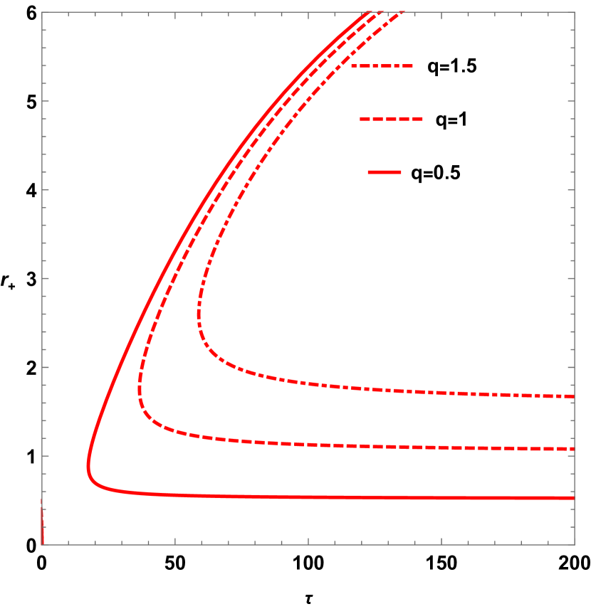
(a) $\alpha=0.1$, $b=1$, $k=1$, and $\Lambda=0.01$.

(b) $q=0.5$, $b=1$, $k=1$, and $\Lambda=0.01$.

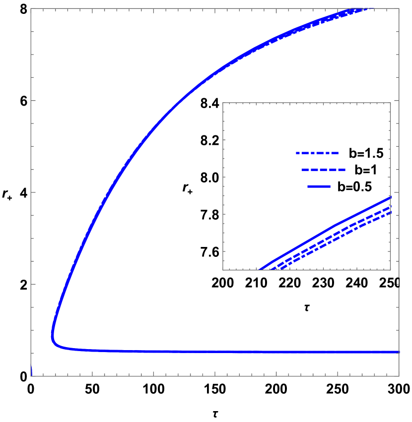
(c) $q=0.5$, $\alpha=0.1$, $k=1$, and $\Lambda=0.01$.

Figure 4: Variation of $\tau$ vs $r_{+}$ plots for topological charged dilaton black holes $(k=1)$ with different thermodynamic parameters.

When considering a negative value of $\Lambda$ (AdS spacetime), we observe that these black holes can be categorized into two topological classes with topological charges of either $0$ or $1$, depending on the value of $\alpha$. Interestingly, the phase transition properties vary with changes in $\alpha$. For smaller values of $\alpha$ (close to zero), these black holes exhibit van der Waals-like phase transition. At $\alpha=0$, the black holes mimic the characteristics of Reissner-Nordstrom (RN) charged AdS black holes. As the value of $\alpha$ increases, only the Davies-type phase transition is observed. Consequently, the thermodynamic topology of these black holes changes with the increasing value of $\alpha$. In Fig. 5 and Fig. 6, we plot $\tau$ vs $r_{+}$ for two values of $\alpha$ for example, while keeping $q=2$, $b=1$, $\Lambda=-0.01$, and $k=1$. In Fig. 5(a) for $\alpha=0.15$, we can clearly see three black hole branches. Vector plots in Fig. 5(b), Fig. 5(c) and Fig. 5(d), represent the zero point in the $(r,\theta)$ plane for $\tau=75$. There are three zero points: $(2.9375,\frac{\pi}{2})$ in the small black hole branch (SBH), $(6.2419,\frac{\pi}{2})$ in the intermediate black hole branch (IBH) and $(17.9060,\frac{\pi}{2})$ in the large black hole branch (LBH). Next, we will calculate the winding number for all three branches at the zero points mentioned above and by adding them we will obtain the total topological charge. It is found that the small black hole (SBH) branch, depicted by the black solid line in the range $0\leq r_{+}\leq 3.9272$, has a winding number of $+1$. The intermediate black hole branch, shown by the blue dashed line for $3.9272<r_{+}\leq 11.3159$, has a winding number of $-1$. The large black hole branch, represented by the red solid line for $r_{+}>11.3159$, also has a winding number of $+1$. These winding numbers are illustrated in Fig. 5(e). The winding numbers indicate that both the large and small black hole branches are stable (with a winding number of $+1$), while the intermediate black hole branch is unstable (with a winding number of $-1$). Consequently, the total topological charge is $W=1-1+1=1$. Moreover, for this value of $\alpha$, we observe an annihilation point at $r_{+}=3.9272$ and a generation point at $r_{+}=11.3159$. Then, we consider $\alpha=0.49$ and keep the rest of the value the same as the above scenario.

In Fig. 6(a), we observe two black hole branches: a stable small black hole branch with winding number $+1$ and an unstable large black hole branch with winding number $-1$. An annihilation point is observed at $r_{+}=7.5278$ The total topological charge is found to be $W=-1+1=0.$. Thus, it can be inferred that the topological charge changes with variations in the value of $\alpha$. However, other thermodynamic parameters are found to have no impact on the topological charge.

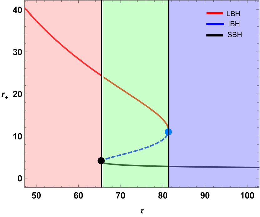
(a)

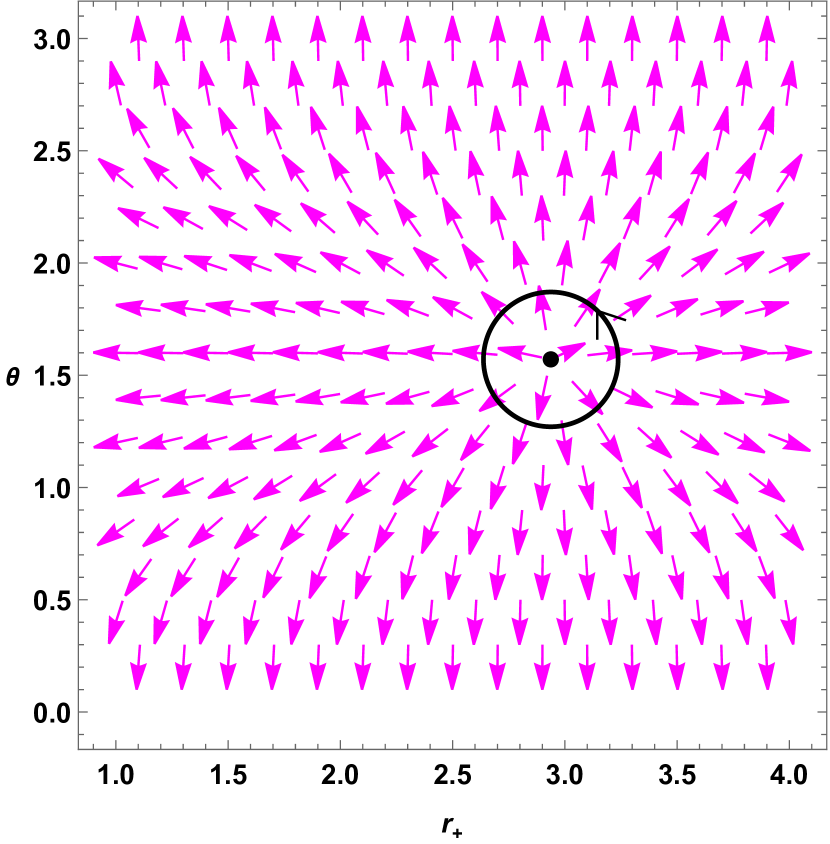
(b)

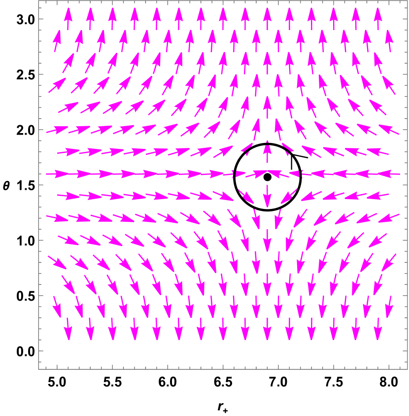
(c)

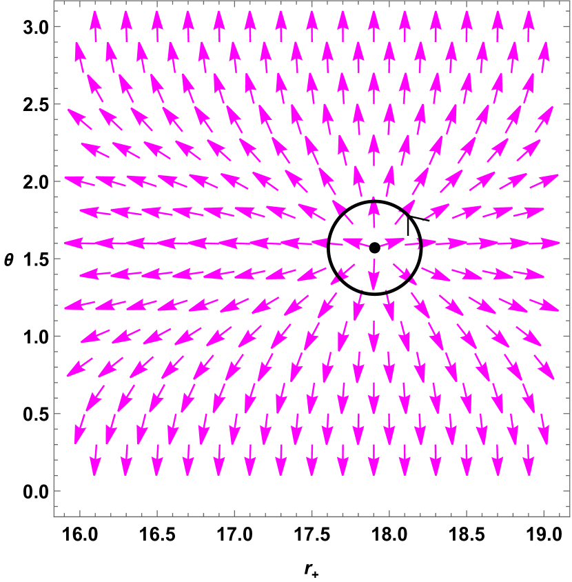
(d)

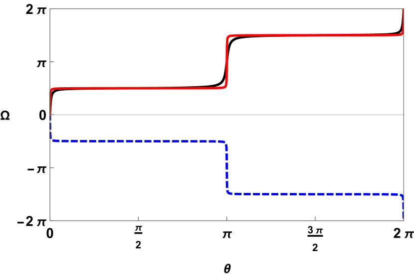
(e)

Figure 5: Fig. 5(a), represents $\tau$ vs $r_{+}$ plot for $q=2$, $b=1$, $\Lambda=-0.01$, $k=1$, and $\alpha=0.15$. Fig. 5(b), Fig. 5(c), and Fig. 5(d) shows vector plot for zero points $r_{+}=2.9375$, $r_{+}=6.2419$, $r_{+}=17.9060$, respectively. The winding number calculations for zero points $r_{+}=2.9375$, $r_{+}=6.2419$, $r_{+}=17.9060$ are represented by black solid line, blue dashed line, red solid line respectively in Fig. 5(e).

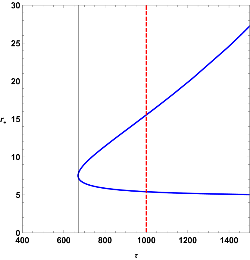
(a)

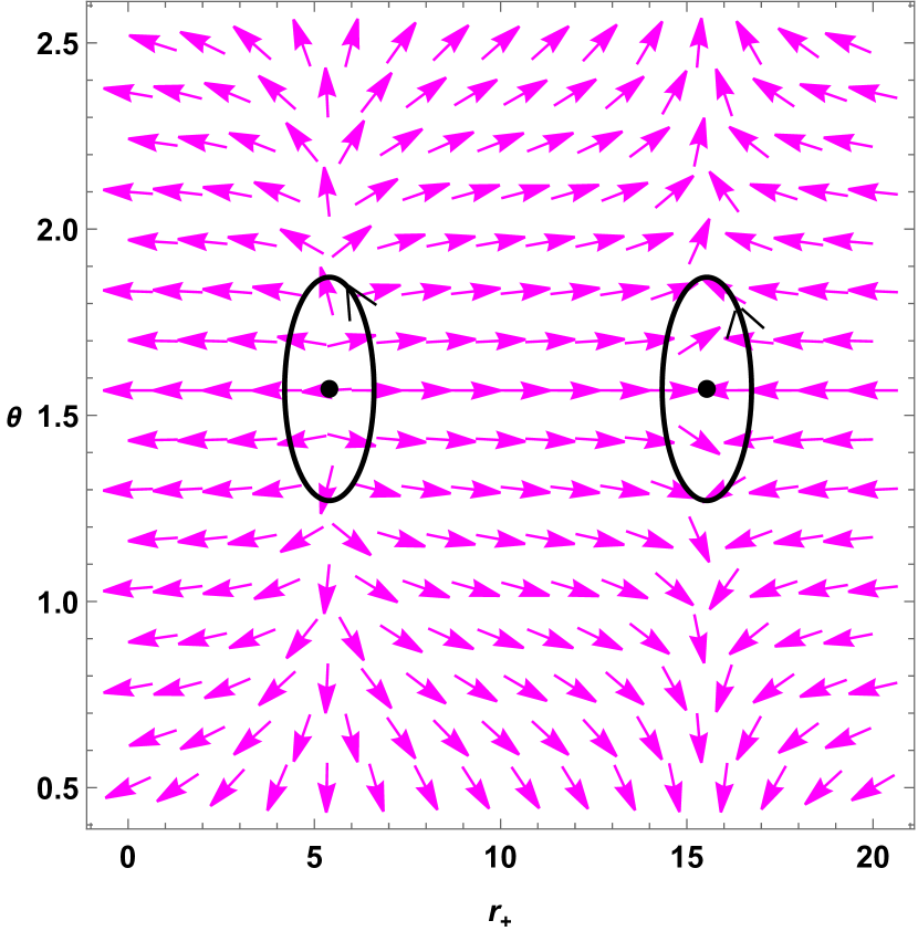
(b)

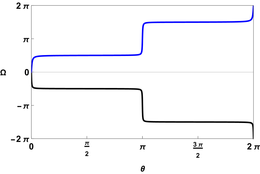
(c)

Figure 6: Fig. 6(a) is the $\tau$ vs $r_{+}$ plot for $\alpha=0.49$ and $q=2$, $b=1$, $\Lambda=-0.01$, $k=1$. Fig. 6(b) is the vector plot in the $r-\theta$ plane for $\tau=1000$. As it is clear from the vector plot, the zero point is found to be at $(5.4030,\frac{\pi}{2})$ in the small black hole branch and $(15.5381,\frac{\pi}{2})$ in the large black hole branch. In Fig. 6(c), the blue contour represents winding number for large black hole branch and black contour represents the same for small black hole branch.

In Fig. 7, the impact of $\alpha$ on topological charge is shown. It is observed that, apart from $\alpha$ and sign of $\Lambda$, the topological charge is independent of other thermodynamic parameters. In conclusion, for topological charged dilatonic black holes with $k=1$ in the fixed charge ensemble, the topological charge is $0$ in dS spacetime and $0$ or $1$ in AdS spacetime depending on the value of $\alpha$.

b!

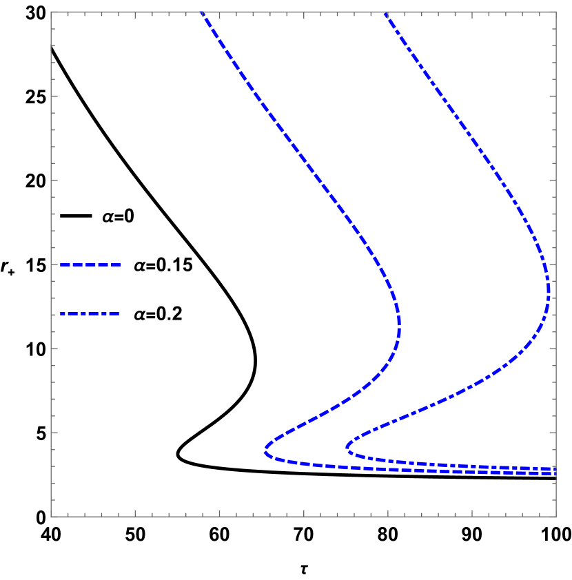
(a) W=1

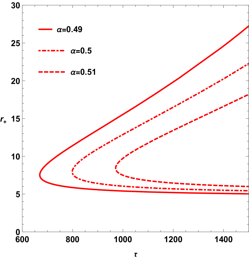
(b) W=0

Figure 7: $\tau$ vs $r_{+}$ plot for different values $\alpha$ while keeping $q=2$, $b=1$, $\Lambda=-0.01$, and $k=1$ fixed. $W$ denotes the winding number for the plots.

IV.1.2 For hyperbolic ($k=-1$) curvature hypersurface

For topological charged dilatonic black holes with constant $t$ and $r$ boundaries, characterized by a hypersurface with hyperbolic curvature, the equation for $\tau$ can be derived by substituting $k=-1$ into Eq. (35), which is

$$\tau_{k=-1}=\frac{4\pi r_{+}^{3}\left(\frac{b}{r_{+}}\right)^{\frac{-2\alpha^{2}}{\mathcal{K}_{1,1}}}}{\frac{\mathcal{K}_{3,-1}r_{+}^{2}}{\mathcal{K}_{-1,1}}-\frac{\mathcal{K}_{1,1}\mathcal{K}_{5,-3}\Lambda r_{+}^{4}\left(\frac{b}{r_{+}}\right){}^{\frac{4\alpha^{2}}{\mathcal{K}_{1,1}}}}{\mathcal{K}_{1,-3}}-q^{2}\mathcal{K}_{5,1}},$$ (36)

From the above equation, it is clear that, because of the requirement for a positive temperature, $\Lambda$ must be negative. We found two topological classes for these kinds of black holes. One with topological charge $+1$ which has a single branch in $\tau$ vs $r_{+}$ plot and another topological class with charge $0$ which contains one stable small black hole branch (winding number$=1$) and an unstable black hole branch (winding number$=-1$). Figs. 8 and 9 demonstrate the different topological class exhibited by these black holes.

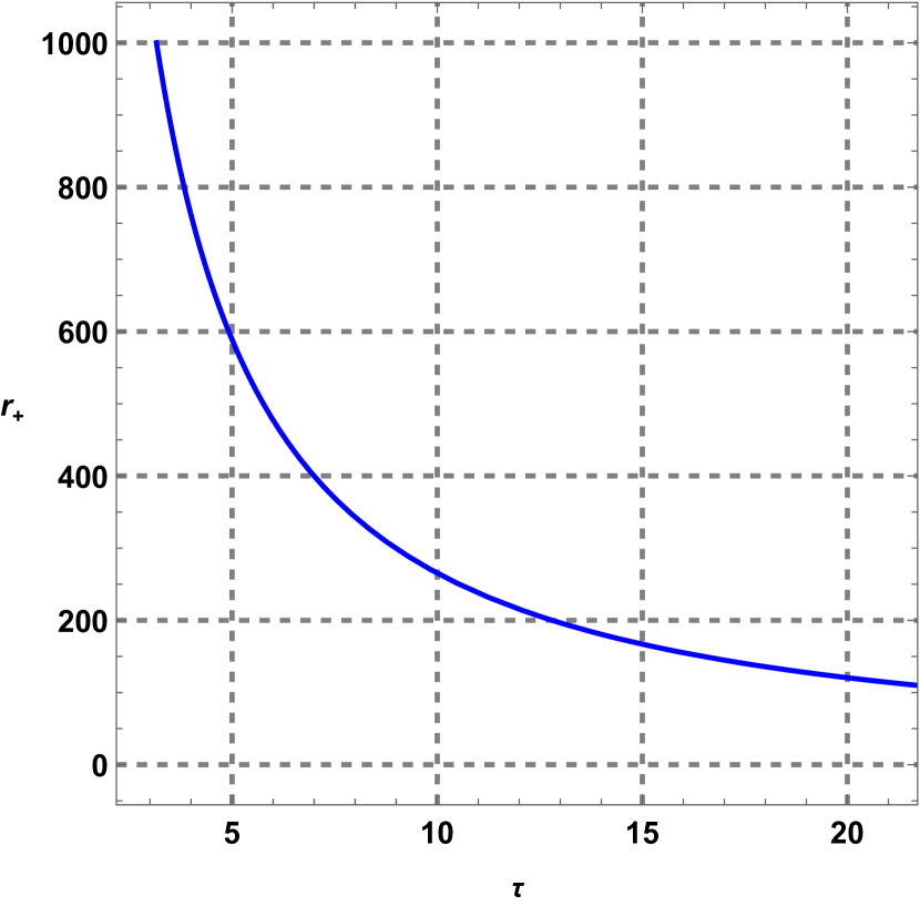
(a)

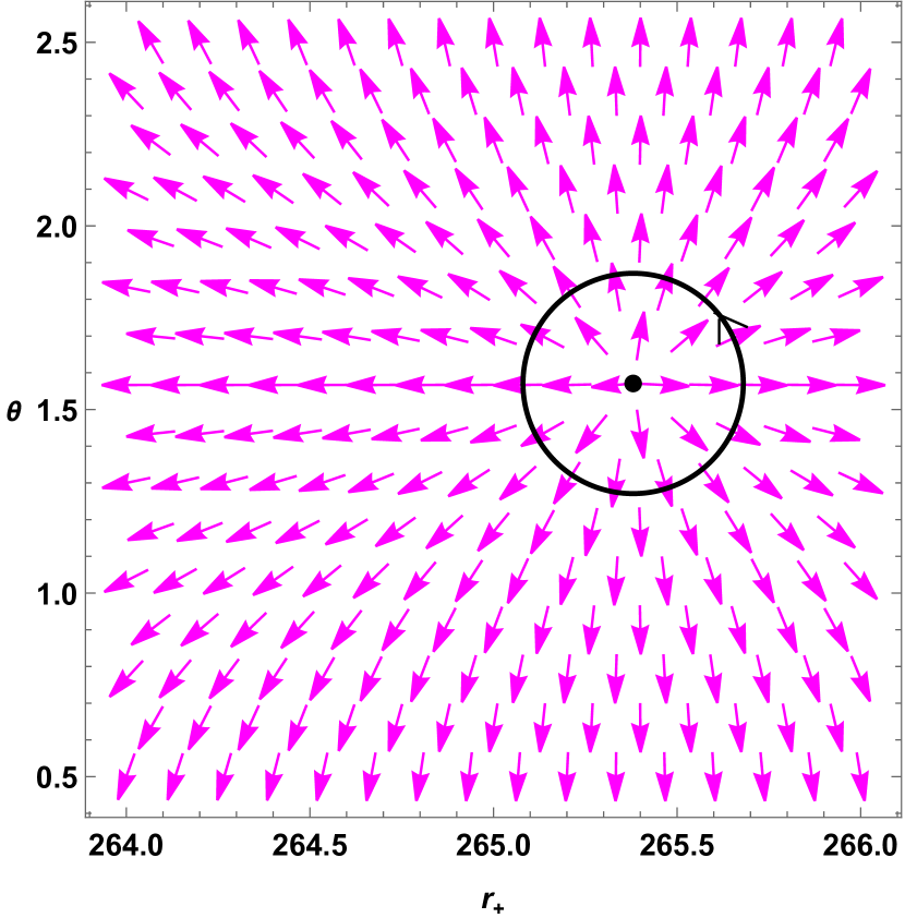
(b)

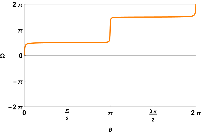
(c)

Figure 8: Fig. 8(a) is the $\tau$ vs $r_{+}$ plot for $\alpha=0.15$ and $q=2$, $b=1$, $\Lambda=-0.01$, $k=-1$. Fig. 8(b) is the vector plot in the $r_{+}-\theta$ plane for $\tau=10$. As it is clear from the vector plot, the zero point is found to be at $(265.3804,\frac{\pi}{2})$. In Fig. 8(c), the orange contour represents the winding number for the black hole, which equals $1$.

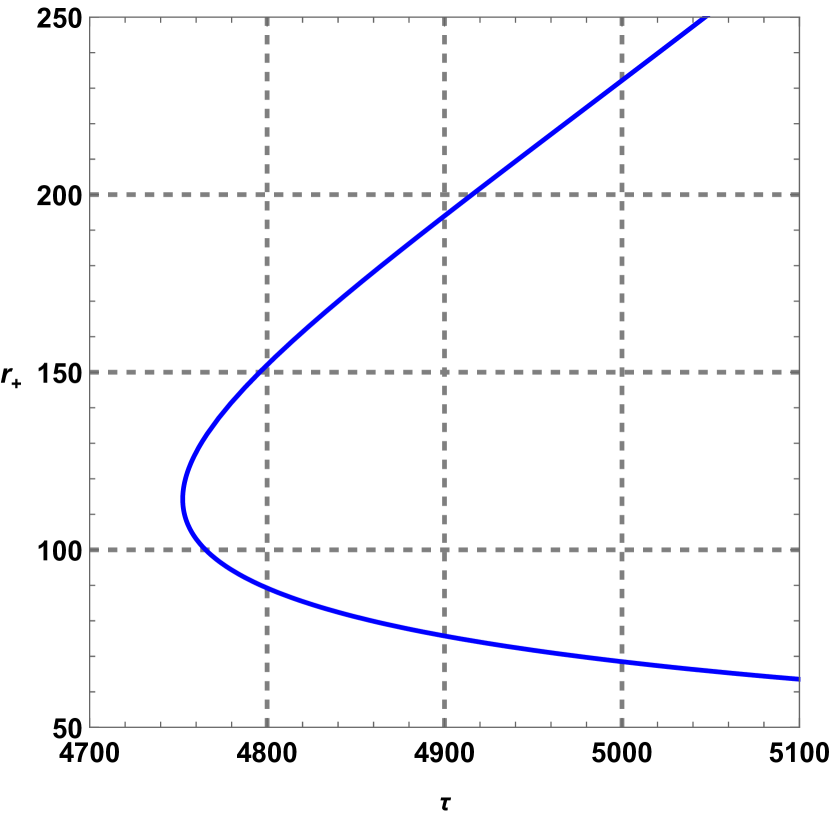
(a)

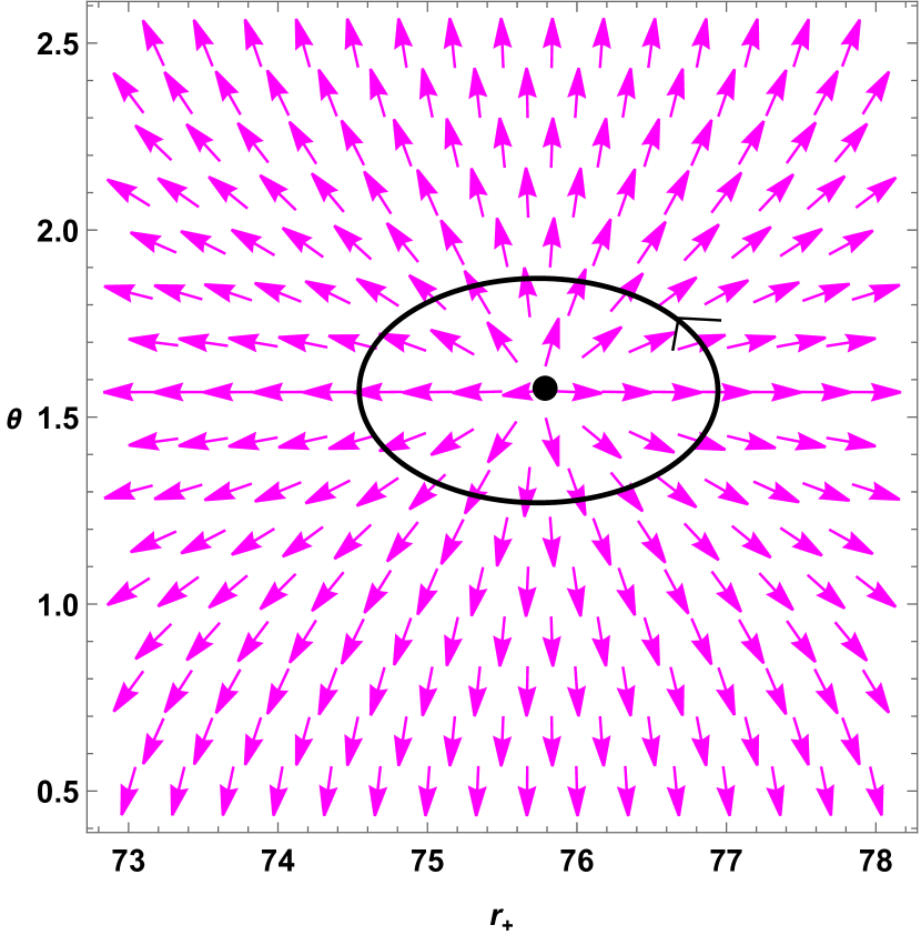
(b)

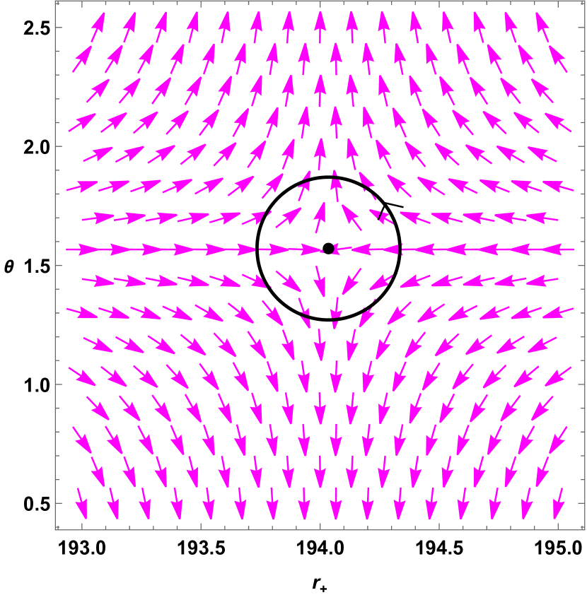
(c)

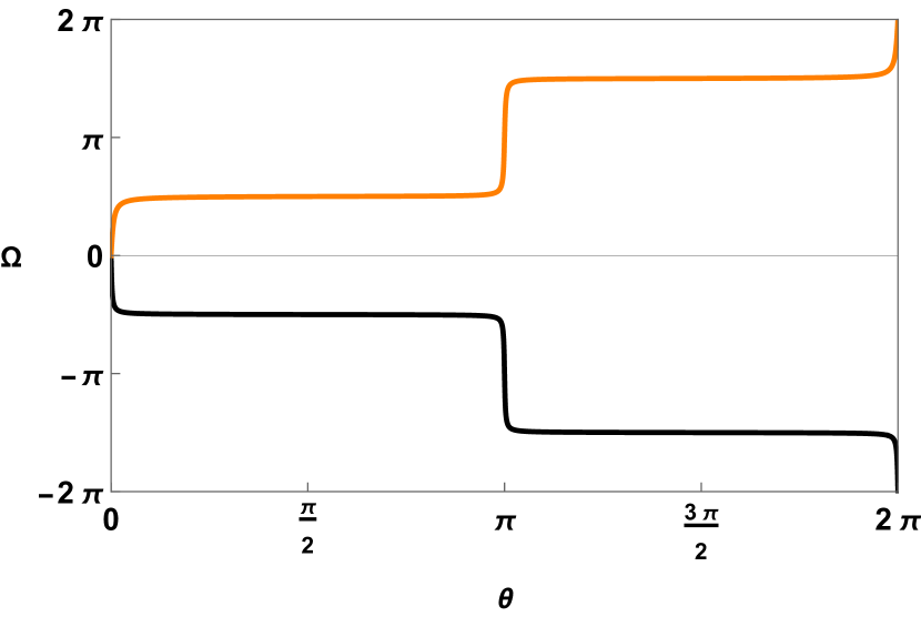
(d)

Figure 9: Fig. 9(a) is the $\tau$ vs $r_{+}$ plot for $\alpha=0.5$ and $q=2$, $b=1$, $\Lambda=-0.01$, $k=-1$. Fig. 9(b) and Fig. 9(c) are the vector plot in the $r_{+}-\theta$ plane for $\tau=4900$. As it is clear from the vector plots, the zero points are found to be at $(75.7431,\frac{\pi}{2})$ in the small black hole branch and $(194.0352,\frac{\pi}{2})$ in the large black hole branch. In Fig. 9(d), the orange contour represents the winding number for the small black hole branch and the black contour represents the same for the large black hole branch.

IV.1.3 For flat ($k=0$) curvature hypersurface

Substituting $k=0$ in Eq. (35), the expression of $\tau$, for topological charged dilatonic black holes with the boundary of $t=$ constant and $r=$constant becomes

$$\tau_{k=0}=\frac{4\pi r_{+}^{3}\left(\frac{b}{r_{+}}\right)^{\frac{-2\alpha^{2}}{\mathcal{K}_{1,1}}}}{-\frac{\mathcal{K}_{1,1}\mathcal{K}_{5,-3}\Lambda r_{+}^{4}\left(\frac{b}{r_{+}}\right){}^{\frac{4\alpha^{2}}{\mathcal{K}_{1,1}}}}{\mathcal{K}_{1,-3}}-q^{2}\mathcal{K}_{5,1}}.$$ (37)

Here also two topological classes of black holes with topological charge $0$ and $+1$ are found depending on the value of $\alpha$. It is important to note that for $k=0$ case also, only negative values of $\Lambda$ are allowed due to positive temperature conditions. Figs. 10 and 11 demonstrate that the different topological classes exhibited by these black holes.

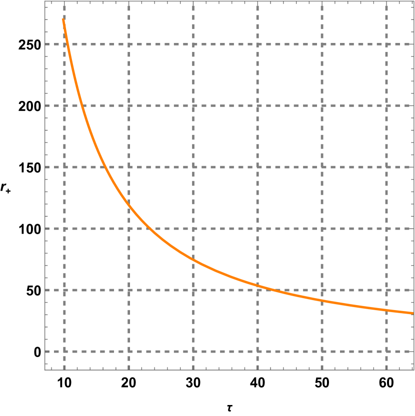
(a)

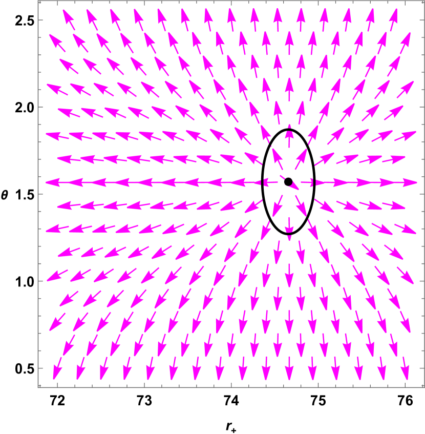
(b)

(c)

Figure 10: Fig. 8(a) is the $\tau$ vs $r_{+}$ plot for $\alpha=0.15$, $q=2$, $b=1$, $\Lambda=-0.01$, and $k=0$. Fig. 8(b) is the vector plot in the $r-\theta$ plane for $\tau=30$. As it is clear from the vector plot, the zero point is found to be at $(74.6558,\frac{\pi}{2})$. In Fig. 8(c), the green contour represents the winding number for the black hole, which equals $1$.

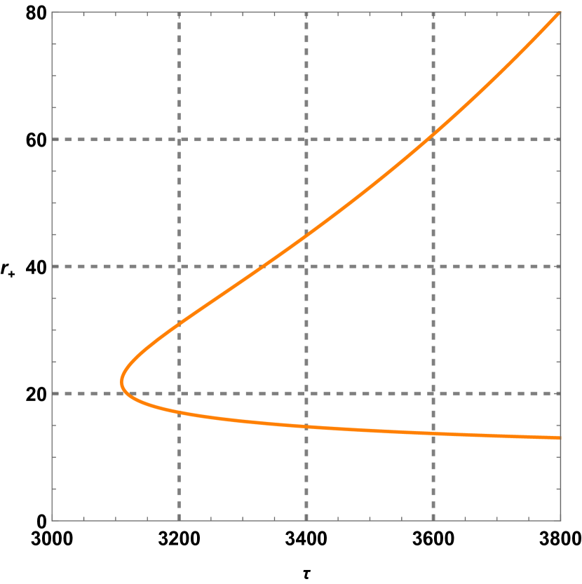
(a)

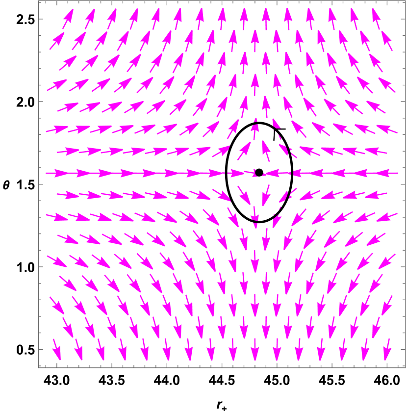
(b)

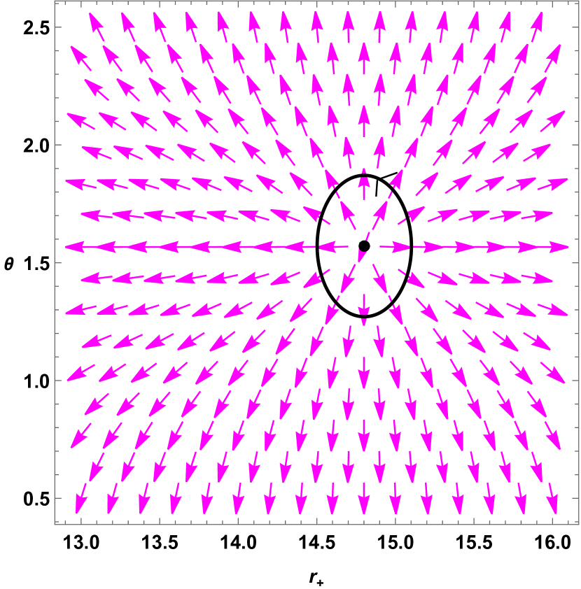
(c)

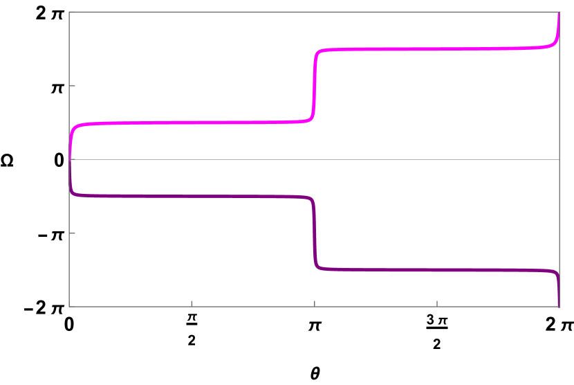
(d)

Figure 11: Fig. 9(a) is the $\tau$ vs $r_{+}$ plot for $\alpha=0.5$, $q=2$, $b=1$, $\Lambda=-0.01$, and $k=0$. Fig. 9(b) and Fig. 9(c) are the vector plot in the $r-\theta$ plane for $\tau=3400$. As it is clear from the vector plots, the zero points are found to be at $(14.8022,\frac{\pi}{2})$ in the small black hole branch and $(44.838,\frac{\pi}{2})$ in the large black hole branch. In Fig. 9(d), the purple contour represents the winding number for a large black hole branch and the magenta contour represents the same for a small black hole branch.

IV.2 Fixed potential ($\phi$) ensemble

In the fixed potential $\phi$ ensemble, the potential $\phi$ is held constant, serving as the conjugate to the charge $q$. The expression for $\phi$ is derived in the following form

$$\phi=\frac{\partial M}{\partial q}=\frac{q\left(\frac{b}{r_{+}}\right){}^{\frac{4\alpha^{2}}{\mathcal{K}_{1,1}}}}{4\pi r_{+}},$$ (38)

where $q$ can be extracted from the Eq. (38) as

$$q=4\pi\phi\left(\frac{b}{r_{+}}\right){}^{-\frac{4\alpha^{2}}{\mathcal{K}_{1,1}}}r_{+}.$$ (39)

Substituting $q$ from Eq. (39) in the expression of mass in Eq. (19), new mass in this ensemble is obtained as

$$\tilde{M}=\frac{\left(\frac{b}{r_{+}}\right){}^{\frac{4\alpha^{2}}{\mathcal{K}_{1,1}}}}{8\pi}\left(16\pi^{2}\phi^{2}r_{+}+\frac{\mathcal{K}_{1,1}\Lambda r_{+}^{3}\left(\frac{b}{r_{+}}\right){}^{\frac{4\alpha^{2}}{\mathcal{K}_{1,1}}}}{\mathcal{K}_{1,-3}}-\frac{kr_{+}}{\mathcal{K}_{1,-1}}\right).$$ (40)

The free energy formula in this ensemble is modified as follows

$$\mathcal{F}=\tilde{M}-\frac{S}{\tau}-q\phi,$$ (41)

using Eqs. (16), (39), (40), and (41) the free energy is obtained as

$$\mathcal{F}=-\frac{\left(\frac{b}{r_{+}}\right){}^{\frac{2\alpha^{2}}{\mathcal{K}_{1,1}}}r_{+}^{2}}{4\tau}+\frac{\left(-\frac{k\left(\frac{b}{r_{+}}\right){}^{\frac{4\alpha^{2}}{\mathcal{K}_{1,1}}}}{\mathcal{K}_{1,-1}}+\frac{\mathcal{K}_{1,1}\mathcal{K}_{1,-1}\Lambda r_{+}^{2}}{\mathcal{K}_{1,-1}\mathcal{K}_{1,-3}}\left(\frac{b}{r_{+}}\right){}^{\frac{8\alpha^{2}}{\mathcal{K}_{1,1}}}-\frac{16\pi^{2}\phi^{2}}{\left(\frac{b}{r_{+}}\right){}^{\frac{4\alpha^{2}}{\mathcal{K}_{1,1}}}}\right)r_{+}}{8\pi}.$$ (42)

Following the same prescription shown in the previous sections, the zero points of the $\phi^{r}$ component are obtained as

$$\tau=\frac{4\pi r_{+}}{\frac{\mathcal{K}_{3,-1}k\left(\frac{b}{r_{+}}\right){}^{\frac{2\alpha^{2}}{\mathcal{K}_{1,1}}}}{\mathcal{K}_{1,-1}}-\frac{\mathcal{K}_{1,1}\mathcal{K}_{5,-3}\Lambda r_{+}^{2}\left(\frac{b}{r_{+}}\right){}^{\frac{6\alpha^{2}}{\mathcal{K}_{1,1}}}}{\mathcal{K}_{1,-3}}-\frac{16\pi^{2}\mathcal{K}_{5,1}\phi^{2}}{\left(\frac{b}{r_{+}}\right){}^{\frac{6\alpha^{2}}{\mathcal{K}_{1,1}}}}}.$$ (43)

IV.2.1 For elliptic ($k=1$) curvature hypersurface

For elliptic curvature hypersurface case, we substitute $k=1$ in the expression Eq. (43). In the dS spacetime where $\Lambda$ is positive, we found a new topological class of topological charge $W=-1$ in this ensemble. The graph in Fig. 12(a) depicts the relationship between $\tau$ and $r_{+}$. The parameters used for this plot are: $\phi=0.02$, $\alpha=0.25$, $b=0.2$, $\Lambda=0.01$, and $k=1$. Only a single branch of the black hole is visible. In Fig. 12(b), a vector plot is presented for the components $\phi^{r}$ and $\phi^{\theta}$ with $\tau=40$. The zero points of the vector field are at $r_{+}=1.6390$. Fig. 12(c) shows that the topological charge for $r_{+}=1.6390$ is $-1$, as indicated by the red line.

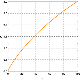
(a)

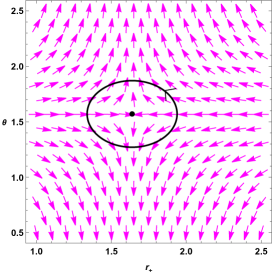
(b)

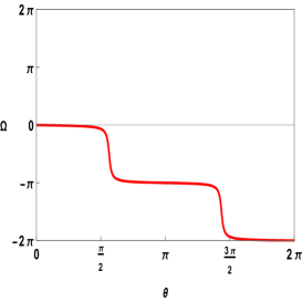
(c)

Figure 12: Topological charge of charged dilatonic black holes ($k=1$) in fixed potential ensemble when positive values of $\Lambda$ are considered.

Next, we consider the negative values of $\Lambda$. In this scenario, although the topological charge is still zero, the stability pattern of black hole branches changes. In previous cases with a topological charge of zero, the small black hole branch was stable with a winding number of $+1$, while the large black hole branch was unstable with a winding number of $-1$. However, as depicted in Fig. 13(a), despite the presence of two branches in the $\tau$ vs $r_{+}$ plot, the smaller black hole now has a winding number of $-1$, and the large black hole branch has a winding number of $+1$, represented by the pink and brown solid lines in Fig. 13(d). These plots were generated using the parameters $\phi=0.02$, $\alpha=0.25$, $b=0.2$, $k=1$, $\Lambda=-0.01$, and $\tau=260$. Unlike the fixed charge ensemble, here we get a generation point which is located at $r_{+}=15.6359$ for the plot Fig. 13(a) represented by the blue dot. In Fig. 13(e), we explicitly demonstrate the change in the stability pattern of the black hole branches by plotting the specific heat $C$ against $r_{+}$. To evaluate $C$ we have used the following formula

$$C=\frac{dM}{dT},$$ (44)

where $T=\frac{1}{\tau}$ for thermodynamically stable black hole branch $C$ is positive, and it is negative for thermodynamically unstable black hole branch. As Fig. 13(e) depicts, the small black hole branch has a negative specific heat and the large black hole branch has a positive specific heat, which explains their stability. The Davies point is located at $r_{+}=15.6359$.

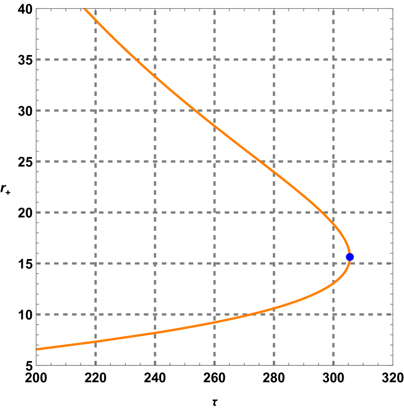
(a)

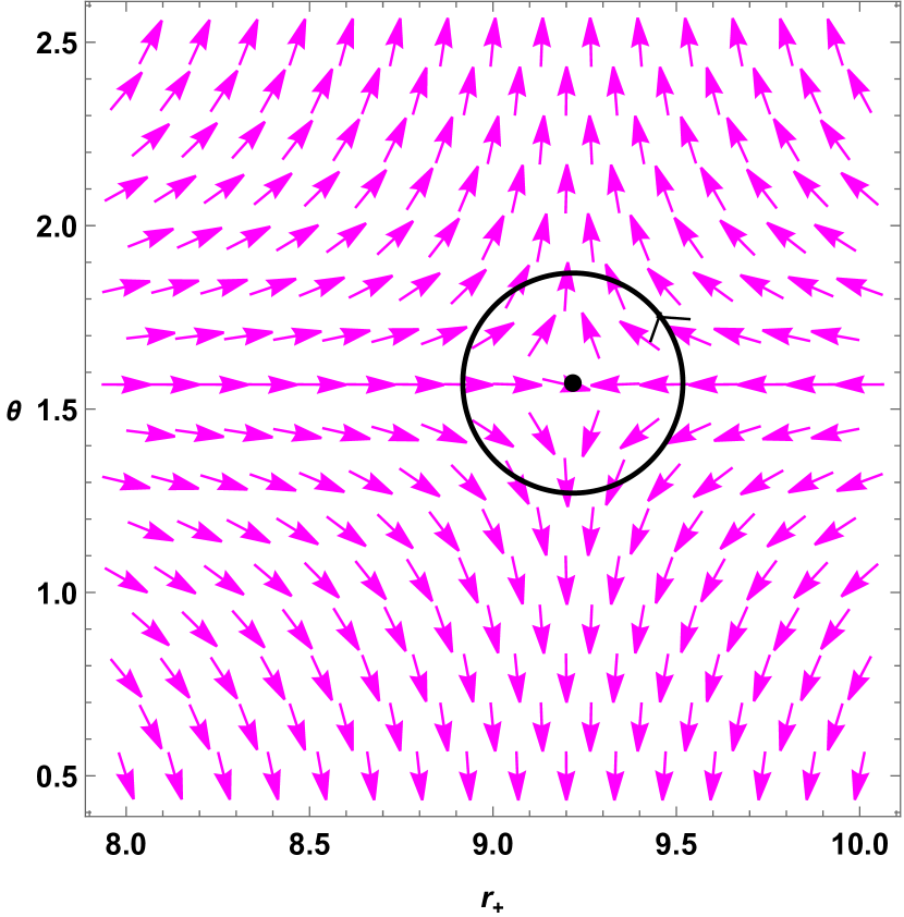
(b)

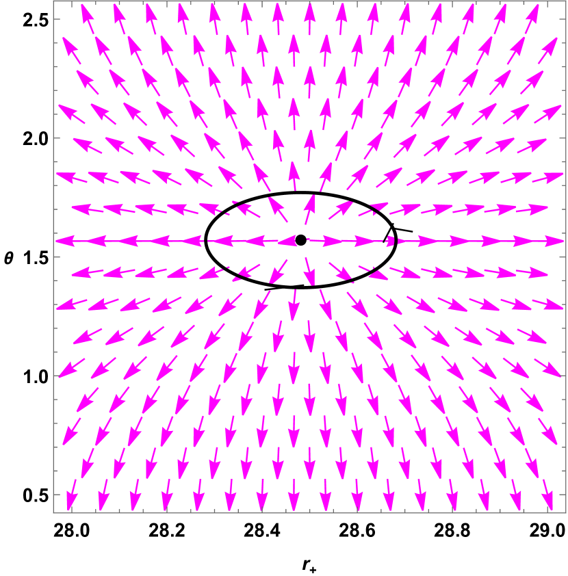
(c)

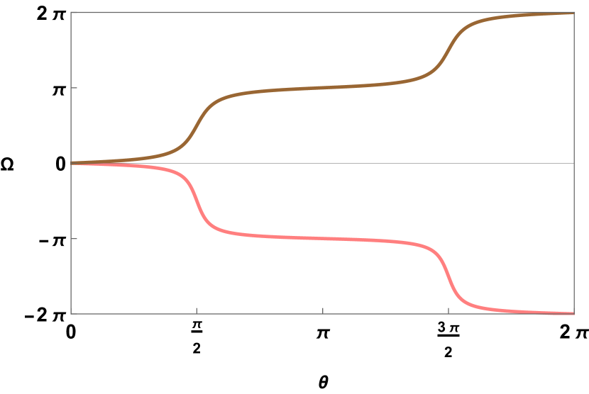
(d)

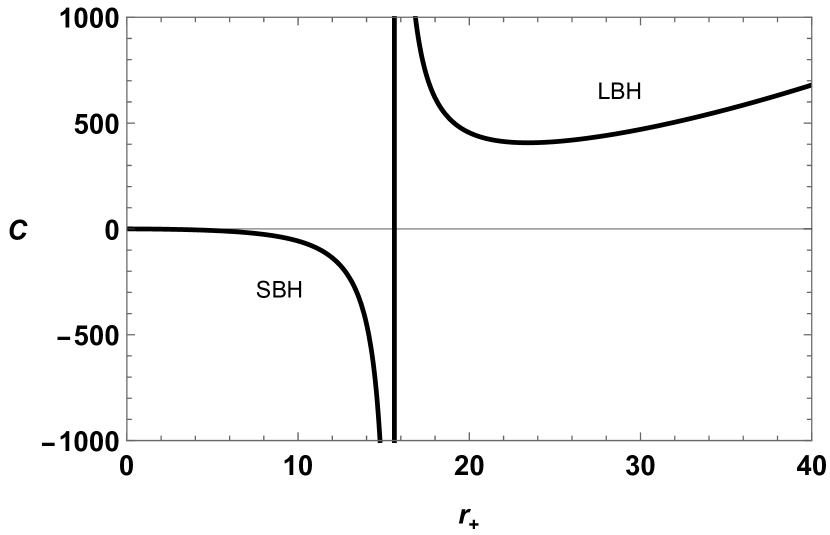
(e)

Figure 13: Fig. 13(a) is the $\tau$ vs $r_{+}$ of topological charged dilatonic black holes with elliptical curvature hypersurface $(k=1)$ in the fixed potential ensemble when the negative value of $\Lambda$ is considered. We have used $\phi=0.02$, $\alpha=0.25$, $b=0.2$, $k=1$, and $\Lambda=-0.01$ for this plot. Fig. 13(b) and Fig. 13(c) are the vector plot in the $r_{+}-\theta$ plane for $\tau=260$. As it is clear from the vector plots, the zero points are found to be at $(9.2178,\frac{\pi}{2})$ in the small black hole branch and $(28.4815,\frac{\pi}{2})$ in the large black hole branch. In Fig. 9(d), the brown contour represents the winding number for the large black hole branch, and the pink contour represents the same for the small black hole branch. As Fig. 13(e) depicts, the small black holes are unstable, whereas the large black holes are stable. In addition, the Davies point is located at $r_{+}=15.6359$.

Another interesting scenario is observed when we increase the value of $\alpha$ while keeping the other parameters constant at $\phi=0.02$, $b=0.2$, $k=1$, and $\Lambda=-0.01$. For example, when we set $\alpha=0.3$, we observe two discontinuous black hole branches, as shown in Fig. 14(a). Besides these two black hole branches, the other branches fall into the negative temperature zone and have therefore been omitted. For the small black hole branch, the winding number is $-1$, while for the large black hole branch, the winding number is $+1$. Consequently, the topological charge is $W=-1+1=0$.

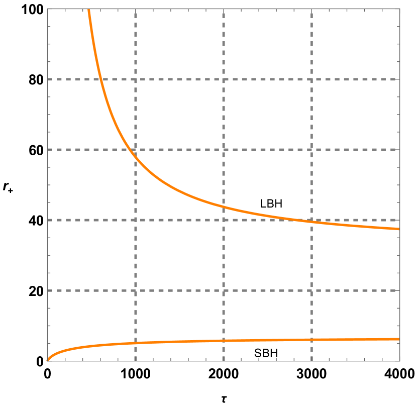
(a)

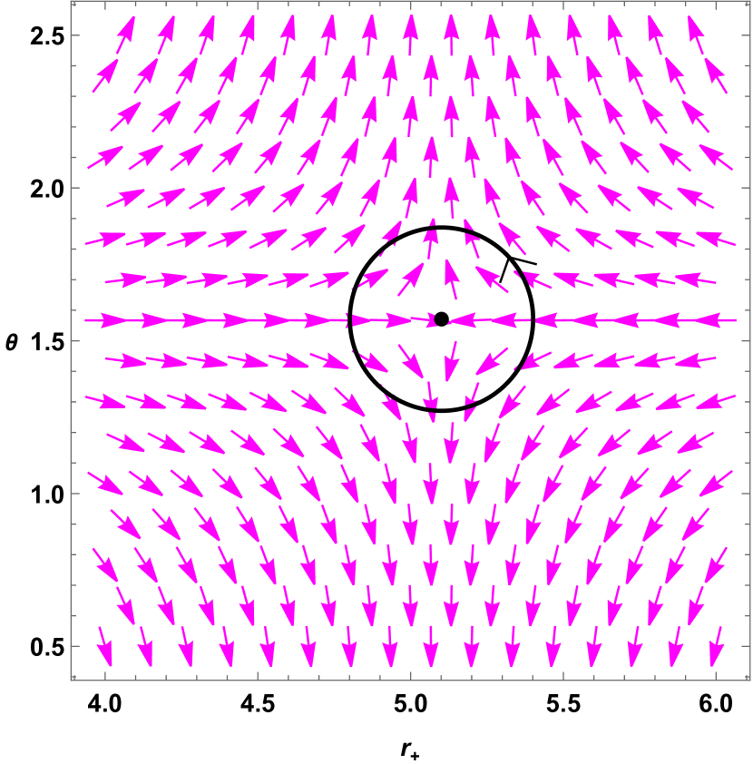
(b)

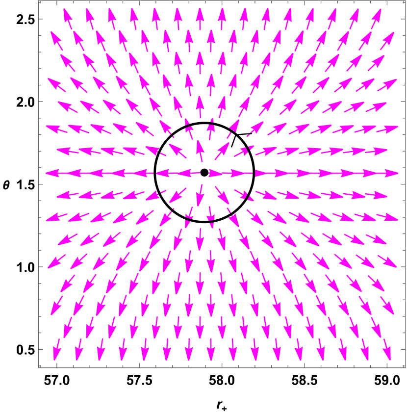
(c)

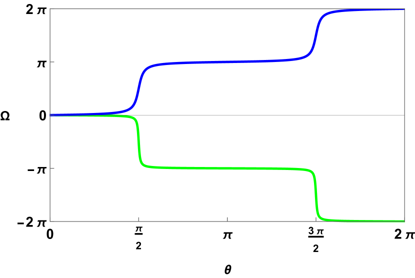
(d)

Figure 14: Fig. 14(a) is the $\tau$ vs $r_{+}$ of charged dilatonic black holes with elliptical curvature hypersurface $(k=1)$ in fixed potential ensemble for $\phi=0.02$, $\alpha=0.25$, $b=0.2$, $k=1$, and $\Lambda=-0.01$. Two black hole branches are observed: a large black hole branch (LBH) and a small black hole branch (SBH). Fig. 14(b) and Fig. 14(c) are the vector plot in the $r_{+}-\theta$ plane for $\tau=1000$. As it is clear from the vector plots, the zero points are found to be at $(5.1010,\frac{\pi}{2})$ in the small black hole branch and $(57.8935,\frac{\pi}{2})$ in the large black hole branch. In Fig. 14(d), the blue contour represents the winding number for the large black hole branch and the green contour represents the same for the small black hole branch.

For this analysis, our concluding remark is as follows: the charged dilatonic black hole with an elliptic ($k=1$) curvature hypersurface has two topological classes, $W=-1$ and $W=0$, in the fixed potential ensemble, depending on the sign of $\Lambda$. Previously, we also identified a topological class with a topological charge of $0$ in the fixed charge ensemble. However, this class is distinct from the $W=0$ class found in the fixed potential ensemble, as the local topology of these classes differs. Although both classes share the same global topology with a topological charge of $W=0$, the stability pattern and the local winding number of the black hole branches differ. Interestingly, in this ensemble, apart from the sign of $\Lambda$, none of the thermodynamic parameters significantly influence the topological charge.

IV.2.2 For hyperbolic ($k=-1$) curvature hypersurface

To evaluate the effect of hyperbolic curvature on the under-studying system, we substitute $k=-1$ in Eq. (43). We find only a single black hole branch (see Fig. 15(a)). The topological charge is $+1$. In this ensemble, we do not get the topological class with topological charge $W=0$ as we have found in the fixed charge ensemble for the black hole with hyperbolic ($k=-1$) curvature hypersurface. Here also, the topological charge is invariant with thermodynamic parameters.

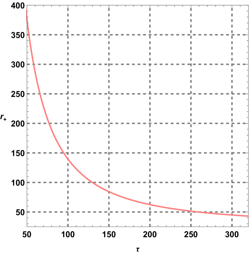
(a)

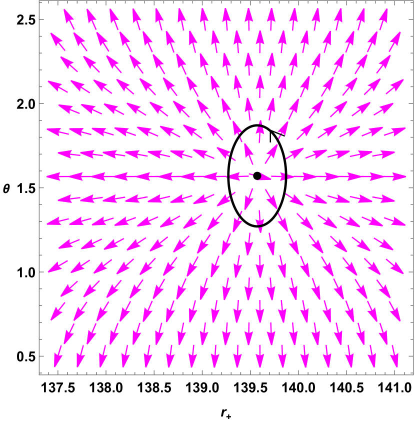
(b)

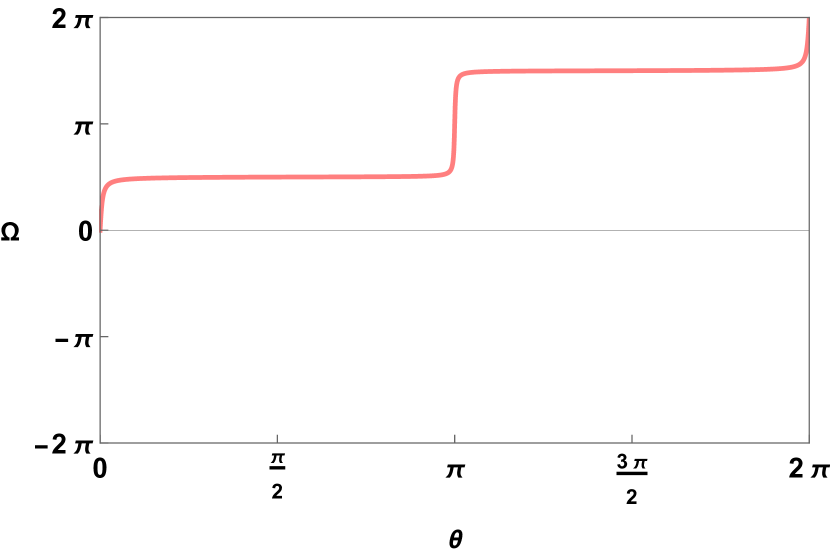
(c)

Figure 15: Fig. 15(a) is the $\tau$ vs $r_{+}$ of the charged dilatonic black holes with hyperbolic curvature hypersurface $(k=-1)$ in fixed potential ensemble for $\phi=0.02$, $\alpha=0.25$, $b=0.2$, $k=-1$, and $\Lambda=-0.01$, where a single black hole branch is observed. Fig. 15(b) is the vector plot in the $r_{+}-\theta$ plane for $\tau=100$. As it is clear from the vector plot, the zero point is found to be at $(139.5713,\frac{\pi}{2})$. In Fig. 15(c), the pink contour represents the winding number for the black hole, which is found to be $W=+1$.

IV.2.3 For flat ($k=0$) curvature hypersurface

We substitute $k=0$ in Eq. (43). In this case, we find only a single black hole branch, as shown in Fig. 16(a). The topological charge is again determined to be $+1$. For these types of black holes also, we do not encounter the topological class with a topological charge of $W=0$, as we found in the fixed charge ensemble. Additionally, the topological charge remains invariant with respect to the thermodynamic parameters.

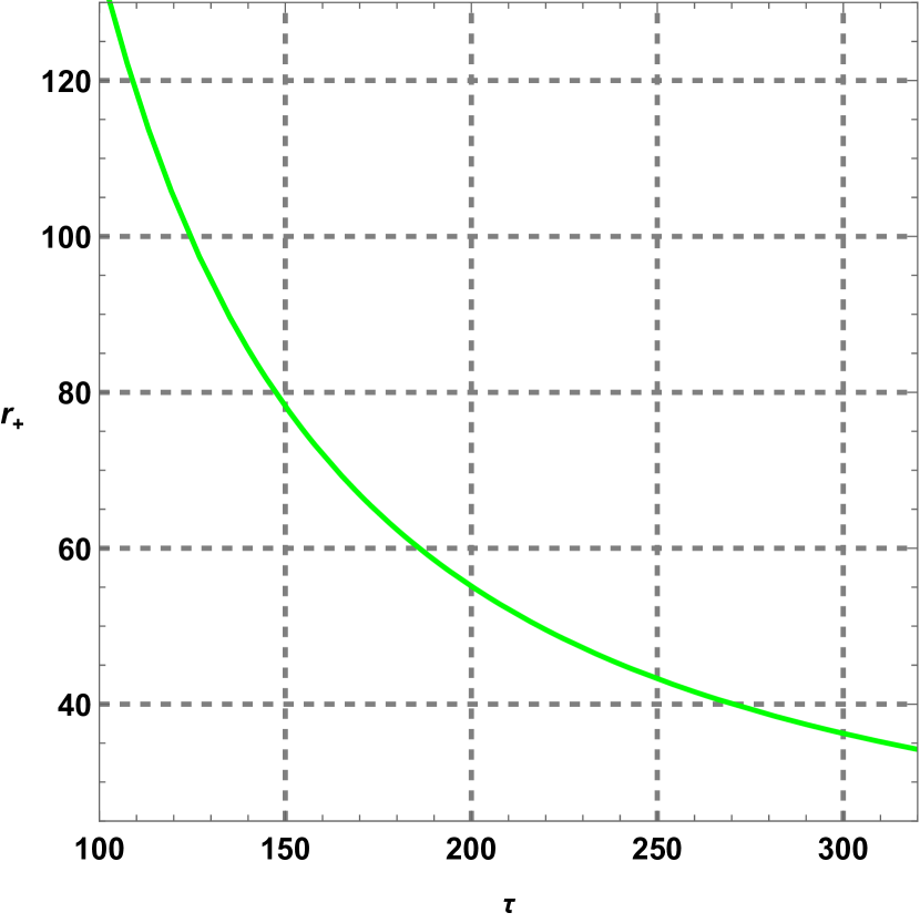
(a)

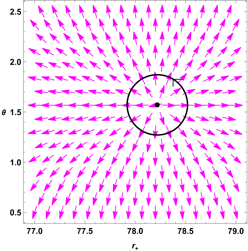
(b)

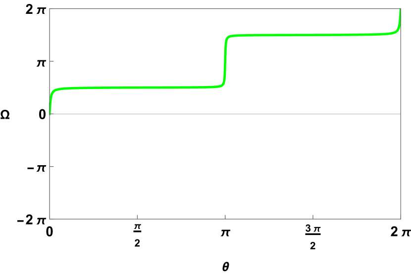
(c)

Figure 16: Fig. 16(a) is the $\tau$ vs $r_{+}$ of charged dilatonic black holes with flat curvature hypersurface ($k=0$) in fixed potential ensemble for $\phi=0.02$, $\alpha=0.25$, $b=0.2$, $k=0$, $\Lambda=-0.01$ where a single black hole branch is observed. Fig. 15(b) is the vector plot in the $r_{+}-\theta$ plane for $\tau=150$. As it is clear from the vector plot, the zero point is found to be at $(78.2196,\frac{\pi}{2})$. In Fig. 15(c), the green contour represents the winding number for the black hole, which is found to be $W=+1$.

Our findings are reported in Table. 1, based on the effect of the topological constant $k$. In other words, the Table. 1 categorizes the results for elliptical ($k=1$), flat ($k=0$), and hyperbolic ($k=-1$) curvature hypersurfaces.

Table 1:

ensembles	$k$	(A)dS spacetime	topological charge	generation point	annihilation point
	$k=1$	dS	$0$	$1$	$0$
fixed $q$ ensemble		AdS	$1$ or $0$	$1$ or $0$	$1$ or $0$
	$k=-1$	AdS	$0$ or $1$	$1$ or $0$	$0$
	$k=0$	AdS	$0$ or $1$	$0$ or $1$	$0$
	$k=1$	dS	$-1$	$0$	$0$
fixed $\phi$ ensemble		AdS	$0$	$0$	$1$
	$k=-1$	AdS	$1$	$0$	$0$
	$k=0$	AdS	$1$	$0$	$0$

V Conclusion

In this paper, we first explored the concept of topological charged dilatonic black holes, which were black holes in dilaton gravity with the presence of the Maxwell field. We calculated the Kretschmann scalar and found that in the presence of the dilaton field, the asymptotic behavior of the spacetime changed. Indeed, black hole spacetimes were neither asymptotically flat nor (A)dS. We then examined the impact of the topological constant ($k$) on the event horizon. Our findings indicated that black holes with a large size corresponded to a negative value of the topological constant, i.e., $k=-1$. Our analysis is presented in Figure. 2, which revealed that for $k=+1$ and $k=0$, the large black holes had a small value of $\alpha$ and a large value of $b$. However, in the case of $k=-1$, the large black holes exhibited large values of $\alpha$ and small values of $b$, which was different from the previous two cases.

In section III, we calculated the thermodynamic and conserved quantities for topological charged dilatonic black holes to study their thermodynamic properties. Additionally, the extracted thermodynamic quantities satisfied the first law of thermodynamics.

In Section IV, we explored the thermodynamic topology of these black holes using the off-shell free energy method. We studied two types of thermodynamic ensembles: the fixed $q$ ensemble and the fixed $\phi$ ensemble. In the fixed $q$ ensemble, we first considered the case of elliptic curvature ($k=+1$) hypersurfaces, taking both de Sitter (dS) and anti-de Sitter (AdS) spacetimes into consideration. For a positive value of $\Lambda$, we identified a single topological class $W=0$ with one annihilation point. The topological charge remained invariant despite variations in all thermodynamic parameters of dilaton gravity. Upon shifting $\Lambda$ to negative values, we discovered two topological classes $W=+1$ and $W=0$. Notably, the topological class of the black hole was dependent on the parameter $\alpha$ of dilaton gravity. Additionally, we found one annihilation point and either one or zero generation points in this scenario. For the cases of flat ($k=0$) and hyperbolic ($k=-1$) curvature hypersurfaces, we identified two topological classes, $W=+1$ and $W=0$, with either one or zero annihilation points. Here, the topological charge also showed dependence on the parameter $\alpha$ of dilaton gravity for topological constants $k=0$ and $k=-1$.

In the fixed potential $\phi$ ensemble, we observed a topological class $W=-1$ in dS spacetime, characterized by a positive cosmological constant ($\Lambda$), and a topological class $W=0$ with a generation point in AdS spacetime, associated with a negative $\Lambda$. Notably, the local thermodynamic topology changes significantly in the fixed $\phi$ ensemble. Previously, in the fixed charge ($q$) ensemble, we also identified a $W=0$ topological class, but its local thermodynamic topology contrasts with that found in the fixed $\phi$ ensemble’s $W=0$ class. Despite having the same topological charge, their winding numbers revealed opposite local topologies.

Similarly, in the fixed charge ensemble for flat ($k=0$) and hyperbolic ($k=-1$) curvature hypersurfaces, we found only one topological class, $W=+1$, which lacked annihilation and generation points. Conversely, in the fixed $\phi$ ensemble, the topological charge remained invariant despite variations in all thermodynamic parameters of dilaton gravity.

In summary, we identified three distinct topological classes, $W=+1$, $0$, $-1$, for charged topological (A)dS black holes in dilaton gravity across different ensembles, contingent upon the values of the topological constant $k$, parameter $\alpha$, and the sign of the cosmological constant $\Lambda$. These findings are synthesized in Table. 2, which also includes thermodynamic topological properties of Reissner-Nordstrom (RN) black holes for comparison (Ref. [64]).

Table 2:

Ensembles	Topological Properties	topological charged dilatonic black holes	RN black holes
	Topological Charge	$0$ or $1$	$0$ or $1$
Fixed charge $(q)$ ensemble	Generation Point	$0$ or $1$	$0$ or $1$
	Annihilation Point	$0$ or $1$	$0$ or $1$
	Topological Charge	$-1$, $0$ or $1$	$-1$, $0$
Fixed potential $(\phi)$ ensemble	Generation Point	$1$ or $0$	$1$ or $0$
	Annihilation Point	$1$ or $0$	$0$

- [1] S. Weinberg, Rev. Mod. Phys. 61, 1 (1989).
- [2] A. G. Riess, et al. (Supernova Search Team), Astron. J 116, 1009 (1998).
- [3] S. Perlmutter, et al. (Surpernova Cosmoly Project), Astrophys. J 517, 565 (1999).
- [4] D. N. Spergel et al. [WMAP], Astrophys. J. Suppl. 148, 175 (2003).
- [5] P. A. R. Ade, et al. [Planck], Astron. Astrophys. 594, A13 (2016).
- [6] R. Dick, [arXiv:hep-th/9609190 (1996)].
- [7] Y. M. Cho, Phys. Rev. D 41, 2462 (1990).
- [8] Z. G. Huang, H. Q. Lu, and W. Fang, Int. J. Mod. Phys. D 16, 1109 (2007)
- [9] Z. G. Huang, and X. M. Song, Astrophys. Space Sci. 315, 175 (2008).
- [10] T. Koikawa, and M. Yoshimura, Phys. Lett. B 189, 29 (1987).
- [11] G.W. Gibbons, and K. Maeda, Nucl. Phys. B 298, 741 (1988).
- [12] D. Brill, and J. Horowitz, Phys. Lett. B 262, 437 (1991).
- [13] D. Garfinkle, G.T. Horowitz, and A. Strominger, Phys. Rev. D 43, 3140 (1991).
- [14] G. T. Horowitz, and A. Strominger, Nucl. Phys. B 360, 197 (1991).
- [15] R. Gregory, and J. A. Harvey, Phys. Rev. D 47, 2411 (1993).
- [16] S. Mignemi, and D. L. Wiltshire, Phys. Rev. D 46, 1475 (1992).
- [17] S. J. Poletti, J. Twamley, and D. L. Wiltshire, Phys. Rev. D 51, 5720 (1995).
- [18] R. G. Cai, J. Y. Ji, and K. S. Soh, Phys. Rev. D 57, 6547 (1998).
- [19] G. Clement, D. Galtsov, and C. Leygnac, Phys. Rev. D 67, 024012 (2003).
- [20] S. H. Hendi, J. Math. Phys. 49, 082501 (2008).
- [21] C. J. Gao, and S. N. Zhang, Phys. Lett. B 605, 185 (2005).
- [22] S. H. Hendi, A. Sheykhi, and M. H. Dehghani, Eur. Phys. J. C 70, 703 (2010).
- [23] T. Tamaki, and T. Torii, Phys. Rev. D 62, 061501R (2000).
- [24] R. Yamazaki, and D. Ida, Phys. Rev. D 64, 024009 (2001).
- [25] S. S. Yazadjiev, Phys. Rev. D 72, 044006 (2005).
- [26] M. H. Dehghani, A. Sheykhi, and S. H. Hendi, Phys. Lett. B 659, 476 (2008).
- [27] H. S. Liu, H. Lu, and C. N. Pope, Phys. Rev. D 92, 064014 (2015).
- [28] S. H. Hendi, M. Faizal, B. Eslam Panah, and S. Panahiyan, Eur. Phys. J. C 76, 296 (2016).
- [29] J. X. Mo, G. Q. Li, and X. B. Xu, Phys. Rev. D 93, 084041 (2016).
- [30] H. Quevedo, M. N. Quevedo, and A. Sanchez, Phys. Rev. D 94, 024057 (2016).
- [31] A. C. Li, H. Q. Shi, and D. F. Zeng, Phys. Rev. D 97, 026014 (2018)
- [32] B. Eslam Panah, S. H. Hendi, S. Panahiyan, and M. Hassaine, Phys. Rev. D 98, 084006 (2018).
- [33] M. Azreg-Ainou, S. Haroon, M. Jamil, and M. Rizwan, Int. J. Mod. Phys. D 28, 1950063 (2019).
- [34] R. Brito, and C. Pacilio, Phys. Rev. D 98, 104042 (2018).
- [35] M. M. Stetsko, Eur. Phys. J. C 79, 244 (2019).
- [36] J. L. Blazquez-Salcedo, S. Kahlen, and J. Kunz, Eur. Phys. J. C 79, 1021 (2019).
- [37] A. Dehyadegari, and A. Sheykhi, Phys. Rev. D 102, 064021 (2020).
- [38] H. C. D. Lima Junior, et al., [arXiv:2112.10802].
- [39] M. Y. Zhang, H. Chen, H. Hassanabadi, Z. W. Long, and H. Yang, Chin. Phys. C 47 045101 (2023).
- [40] K. Boshkayev, G. Suliyeva, V. Ivashchuk, and A. Urazalina, Eur. Phys. J. C 84, 19 (2024).
- [41] S. W. Hawking, Nature. 248, 30 (1974).
- [42] S. W. Hawking, Commun. Math. Phys. 43, 199 (1975).
- [43] J. D. Bekenstein, Phys. Rev. D 7, 2333 (1973).
- [44] J. D. Bekenstein, Phys. Rev. D 9, 3292 (1974).
- [45] J. M. Bardeen, B. Carter and S. W. Hawking, Commun. Math. Phys. 31 (1973) 161.
- [46] E. Witten, Adv. Theor. Math. Phys. 2, 253 (1998).
- [47] S. Ryu, and T. Takayanagi, Phys. Rev. Lett. 96, 181602 (2006).
- [48] D. Kastor, S. Ray, and J. Traschen, Class. Quantum Grav. 26, 195011 (2009).
- [49] D. Kubiznak, and R. B. Mann, J. High Energy Phys. 07, 033 (2012).
- [50] N. Altamirano, D. Kubiznak, and R. B. Mann, Phys. Rev. D 88, 101502 (2013).
- [51] A. M. Frassino, D. Kubiznak, R. B. Mann, and F. Simovic, J. High Energy Phys. 09, 080 (2014).
- [52] R. G. Cai, L. M. Cao, L. Li, and R. Q. Yang, J. High Energy Phys. 09, 005 (2013).
- [53] C. V. Johnson, Class. Quantum Grav. 31, 205002 (2014).
- [54] H. Xu, W. Xu, and L. Zhao, Eur. Phys. J. C 74, 3074 (2014).
- [55] R. A. Hennigar, R. B. Mann, and E. Tjoa, Phys. Rev. Lett. 118, 021301 (2017).
- [56] S. H. Hendi, R. B. Mann, S. Panahiyan, and B. Eslam Panah, Phys. Rev. D 95, 021501(R) (2017).
- [57] M. R. Visser, Phys. Rev. D 105, 106014 (2022).
- [58] T. F. Gong, J. Jiang, and M. Zhang, J. High Energy Phys. 06, 105 (2023)
- [59] Kh. Jafarzade, B. Eslam Panah, and M. E. Rodrigues, Class. Quantum Grav. 41, 065007 (2024).
- [60] S. W. Wei, and Y. X. Liu, Phys. Rev. D 105, 104003 (2022).
- [61] Y. S. Duan, and M. L. Ge, Sci. Sin. 9, 1072 (1979).
- [62] Y. S. Duan, The structure of the topological current, SLAC-PUB-3301/84 (1984).
- [63] P. K. Yerra, and C. Bhamidipati, Phys. Rev. D 105, 104053 (2022).
- [64] S. W. Wei, Y. X. Liu, and R. B. Mann, Phys. Rev. Lett. 129, 191101 (2022).
- [65] M. B. Ahmed, D. Kubiznak, and R. B. Mann, Phys. Rev. D 107, 046013 (2023).
- [66] M. R. Alipour, M. A. S. Afshar, S. N. Gashti, and J. Sadeghi, Phys. Dark Univ. 42, 101361 (2023).
- [67] N. J. Gogoi, and P. Phukon, Phys. Rev. D 107, 106009 (2023).
- [68] N. C. Bai, L. Li, and J. Tao, Phys. Rev. D 107, 064015 (2023).
- [69] D. Wu, and S. Q. Wu, Phys. Rev. D 107, 084002 (2023).
- [70] M.-Y. Zhang, H. Chen, H. Hassanabadi, Z. W. Long, and H. Yang, Eur. Phys. J. C 83, 773 (2023).
- [71] Z. Q. Chen, and S. W. Wei, Nucl. Phys. B 996, 116369 (2023).
- [72] M. Rizwan, and K. Jusufi, Eur. Phys. J. C 83, 944 (2023).
- [73] F. Barzi, H. El Moumni, and K. Masmar, J. High Energy Phys. 42, 63 (2024).
- [74] B. Hazarika, and P. Phukon, Prog. Theor. Exp. Phys. 2024, 043E01 (2024).
- [75] J. Sadeghi, M. A. S. Afshar, S. N. Gashti, and M. R. Alipour, Astropart. Phys. 156, 102920 (2024).
- [76] H. Chen, M. Y. Zhang, H. Hassanabadi, B. C. Lutfuoglu, and Z. W. Long, [arXiv:2403.14730].
- [77] A. Mehmood, and M. U. Shahzad, [arXiv:2310.09907].
- [78] B. Eslam Panah, B. Hazarika, and P. Phukon, [arXiv:2405.20022].
- [79] Z. Q. Chen, and S. W. Wei, [arXiv:2405.07525].
- [80] X. D. Zhu, D. Wu, and D. Wen, [arXiv:2402.15531].
- [81] D. Wu, et al., J. High Energy Phys. 06, 213 (2024).
- [82] K. C. K. Chan, J. H. Horne and R. B. Mann, Nucl. Phys. B 447, 441 (1995).
- [83] M. Ozer, and M. O. Taha, Phys. Rev. D 45, 997 (1992).
- [84] A. Sheykhi, Phys. Rev. D 76, 124025 (2007).
- [85] S. H. Hendi, A. Sheykhi, S. Panahiyan, and B. Eslam Panah, Phys. Rev. D 92, 064028 (2015).
- [86] L. F. Abbott and S. Deser, Nucl. Phys. B 195, 76 (1982).
- [87] R. Olea, J. High Energy Phys. 06, 023 (2005).
- [88] G. Kofinas and R. Olea, Phys. Rev. D 74, 084035 (2006).