Probing axion-like particles in leptonic decays of heavy mesons

Abstract

We study the possibility to find the axion-like particles (ALPs) through the leptonic decays of heavy mesons. There are some deviations between the Standard Model (SM) predictions of the branching ratios of the leptonic decays of mesons and the experimental data. This provides some space for the existence of decay channels where the ALP is one of the products. Three scenarios are considered: first, the ALP is only coupled to one single charged fermion, namely, the quark, the antiquark, or the charged lepton; second, the ALP is only coupled to quark and antiquark with the same strength; third, the ALP is coupled to all the charged fermions with the same strength. The constraints of the coupling strength in different scenarios are obtained by comparing the experimental data of the branching ratios of leptonic decays of $B^{-}$, $D^{+}$, and $D_{s}^{+}$ mesons with the theoretical predictions which are achieved by using the Bethe-Salpeter (BS) method. These constraints are further applied to predict the upper limits of the leptonic decay processes of the $B_{c}^{-}$ meson in which the ALP participates.

I Introduction

In 1977, Peccei and Quinn introduced a new global chiral symmetry Peccei and Quinn (1977a), known as $U(1)_{\rm PQ}$ symmetry, to address the strong CP problem in QCD, that is, the absence of CP violation in the strong interactions and the neutron’s electric dipole moment (EDM) being forbidden. At a energy scale $f_{a}$, such a symmetry is assumed to be spontaneously broken, which results in the appearance of a pseudo-Nambu-Goldstone boson, namely the axion  Peccei and Quinn (1977a, b); Wilczek (1978); Weinberg (1978); Di Luzio et al. (2020), whose mass $m_{a}$ is constrained by the relation $m_{a}\sim\frac{m_{\pi}f_{\pi}}{f_{a}}$, where $m_{\pi}$ and $f_{\pi}$ are the mass and decay constant of pion, respectively. This means that if the energy scale $f_{a}$ is very high, the axion should be extremely light. The condition can be relaxed if we are not just limited to such QCD axion, but consider more general Axion-Like Particles (ALPs) Bauer et al. (2017a); Brivio et al. (2017); Martin Camalich et al. (2020). In such cases, both the PQ symmetry breaking scale $f_{a}$ and the ALP mass $m_{a}$ can be considered as independent parameters.

People are interested in ALPs in many aspects. Theoretically, a large number of ALPs are predicted by string theories Arvanitaki et al. (2010); Cicoli et al. (2012). These particles may play an important role in the evolution of cosmology, most importantly, as a candidate of dark matter Marsh (2016). The cosmological and astronomical observations can set strict constraints on the very light ALPs Irastorza et al. (2011); Adrian et al. (2014); Vinyoles et al. (2015); Gao et al. (2024); Budker et al. (2014); Akerib et al. (2017); Agashe et al. (2023). The phenomenology of ALPs have also been extensively studied at the Large Hadron Collider (LHC) Alonso-Álvarez et al. (2023); Biekötter et al. (2022); Bauer et al. (2017b); Jaeckel and Spannowsky (2016); Aad et al. (2024); Buonocore et al. (2024); Ghebretinsaea et al. (2022); Feng et al. (2018); Biswas (2024). For example, they can be produced by the decays of on-shell Higgs/$Z$ boson Biswas (2024); Bauer et al. (2017a), or participate as off shell mediators in the scattering processes Gavela et al. (2020). At high-luminosity electron-positron colliders, ALPs with mass in the MeV-GeV range can also be explored non-resonantly or resonantly Acanfora (2024); Zhang et al. (2024); Ferber et al. (2023); Abudinén et al. (2020); Merlo et al. (2019); Bonilla et al. (2022), which means they can be produced directly by coupling to the charged leptons or the gauge bosons, or produced through the decays of final mesons. For example, in Ref. Merlo et al. (2019) the production of ALPs at $B$ factories is considered, including the contributions of $e^{+}e^{-}\to\gamma a$ and $e^{+}e^{-}\to\Upsilon\to\gamma a$. Recently, the BESIII experiment Ablikim et al. (2023a) use a data sample of $\psi(3686)$ to get the upper limits of the branching fraction of the decay $J/\psi\to\gamma a$ and set constrains on the coupling $g_{a\gamma\gamma}$ in the mass range of $0.165~{}{\rm GeV}\leq m_{a}\leq 2.84~{}{\rm GeV}$. The fixed target experiments are also promising methods in searching ALPs Ema et al. (2024); Afik et al. (2023); Gil et al. (2024); Coloma et al. (2022); Döbrich (2018); Harland-Lang et al. (2019), as the detectors can extend tens of meters and suitable for the detection of long-lived particles. The ALP productions though $K$ meson decays are usually investigated in such cases  Ema et al. (2024); Afik et al. (2023); Gil et al. (2024).

Except the methods mentioned above, the decays of heavy-flavored mesons also provide a way to probe ALPs. On the one hand, a large number of bottomed and charmed mesons have been produced at $B$ factories and $\tau$-charm factory, respectively, and on the other hand, a larger range of $m_{a}$ can be looked into in the decays of heavy mesons compared with that of $K$ meson. We will focus on the decay processes $h^{-}\to\ell^{-}\not{E}$, where $h^{-}=D^{-},~{}D_{s}^{-},~{}B^{-}$, or $B_{c}^{-}$; $\ell^{-}=e^{-},~{}\mu^{-}$, or $\tau^{-}$; $\not{E}$ represents the missing energy. In the Standard Model, $\not{E}$ is carried away by the antineutrino (see Fig. 1), and the corresponding partial width is

$$\Gamma\left(h^{-}\rightarrow\ell^{-}\bar{\nu}_{\ell}\right)=\frac{G_{F}^{2}}{8\pi}\left|V_{Qq}\right|^{2}f_{h}^{2}M^{3}\frac{m_{\ell}^{2}}{M^{2}}\left(1-\frac{m_{\ell}^{2}}{M^{2}}\right)^{2},$$ (1)

where $G_{F}$ is the Fermi coupling constant, $f_{h}$ is the decay constant of $h$ meson, $V_{Qq}$ is the CKM matrix element, $M$ and $m_{\ell}$ are the masses of the meson and the lepton, respectively, and the neutrino mass is assumed to be zero. If an ALP can also be produced and has long enough lifetime to escape the detector, we will have $\Gamma(h^{-}\to\ell^{-}\not{E})=\Gamma(h^{-}\to\ell^{-}\bar{\nu}_{\ell})+\Gamma(h^{-}\to\ell^{-}\bar{\nu}_{\ell}a)$. Then the experimental results of $h^{-}\to\ell^{-}\not{E}$, which are presented in Table 1, can be used to constrain the coupling between the ALP and SM particles.

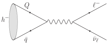
Figure 1: The diagram of two-body leptonic decays of charged heavy meson.

Table 1: Experiment results of ${\mathcal{B}}(B^{-}\to\ell^{-}\not{E})$, ${\mathcal{B}}(D^{-}\to\ell^{-}\not{E})$, and ${\mathcal{B}}(D_{s}^{-}\to\ell^{-}\not{E})$.

Channel	Experiment values
${\mathcal{B}}(B^{-}\to e^{-}\not{E})$	$\leq 9.8\times 10^{-7}$ Satoyama et al. (2007)
${\mathcal{B}}(B^{-}\to\mu^{-}\not{E})$	$(5.3\pm 2.0\pm 0.9)\times 10^{-7}$  Prim et al. (2020)
${\mathcal{B}}(B^{-}\to\tau^{-}\not{E})$	$(7.2\pm 2.7\pm 1.1)\times 10^{-5}$ Hara et al. (2013)
${\mathcal{B}}(D_{s}^{-}\to e^{-}\not{E})$	$\leq 0.83\times 10^{-4}$  Zupanc et al. (2013)
${\mathcal{B}}(D_{s}^{-}\to\mu^{-}\not{E})$	$(0.5294\pm 0.0108\pm 0.0085)\times 10^{-2}$ Ablikim et al. (2023b)
${\mathcal{B}}(D_{s}^{-}\to\tau^{-}\not{E})$	$(5.44\pm 0.17\pm 0.13)\times 10^{-2}$ Ablikim et al. (2023c)
${\mathcal{B}}(D^{-}\to e^{-}\not{E})$	$\leq 8.8\times 10^{-6}$ Eisenstein et al. (2008)
${\mathcal{B}}(D^{-}\to\mu^{-}\not{E})$	$(3.71\pm 2.7\pm 1.1)\times 10^{-3}$  Ablikim et al. (2014)
${\mathcal{B}}(D^{-}\to\tau^{-}\not{E})$	$(1.20\pm 0.24\pm 0.12)\times 10^{-5}$ Medina et al. (2019)

What we will do in this article is inspired by Refs. Aditya et al. (2012); Guerrera and Rigolin (2022, 2023); Gallo et al. (2022) where the processes $h^{-}\to\ell^{-}\bar{\nu}_{\ell}a$ with $a$ being an ALP were studied. Except the pseudoscalar attribution, Ref. Aditya et al. (2012) also considered the possibility that $a$ being a vector particle. Here we will also probe such processes, but with three main differences. First, the hadron transition matrix elements will be calculated by using the Bethe-Salpeter (BS) method which is suitable to the description of heavy mesons. Second, for the coupling of ALP with quarks, we consider the interference effects of different diagrams, and extract the allowed range of parameters in a more general way. Third, we will explore the ALP production from the decays of double heavy meson $B_{c}$, that is $B_{c}^{-}\to\ell^{-}\bar{\nu}_{\ell}a$, which could give the constraint in a more large mass range of ALP.

The paper is organized as follows. In Section II, we write the effective Lagrangian which describes the interaction between ALPs and charged fermions. Then we calculate the hadronic transition matrix elements of the $h^{-}\to\ell^{-}\nu_{\ell}a$ processes by using the BS method. In Section III, we apply the experimental results to extract the allowed regions of the parameters which are then used to calculate the upper limits of the branching fractions of the $B_{c}$ decay processes. Finally, we present the summary in Section IV.

II Theoretical Formalism

Generally, the ALPs can interact both with the fermions and gauge bosons. Here in the case of leptonic decays of heavy mesons, we only consider the tree level diagrams shown in Fig. 2 which represent the interaction of the ALP with SM fermions. The contributions of gauge bosons are of higher order and assumed to be neglected. The effective Lagrangian, which describes flavor conserving processes, consists of dimension-five operators Aditya et al. (2012); Guerrera and Rigolin (2022, 2023); Gallo et al. (2022)

$$\mathcal{L}_{eff}\supset-\frac{\partial_{\mu}a}{2f_{a}}\sum_{i}c_{i}\bar{\psi_{i}}\gamma^{\mu}\gamma_{5}\psi_{i}\Rightarrow i\frac{a}{f_{a}}\sum_{i}c_{i}m_{i}\bar{\psi_{i}}\gamma_{5}\psi_{i},$$ (2)

where $c_{i}$ is the effective coupling constant with the index $i$ extending over all the fermions. As Refs. Guerrera and Rigolin (2022, 2023); Gallo et al. (2022) did, in the last step we have used the equation of motion to rewrite the expression. This corresponds to the use of another operator basis, which will lead to the different upper limits of $c_{i}$. However, when we calculate the decay channels of $B_{c}$ meson, two methods give quite close results. The dependence of the fermion mass $m_{i}$ indicates that the ALP does not couple directly with the neutrinos and Fig. 2(d) needs not to be taken into account, which will simplify the calculation.

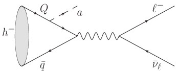
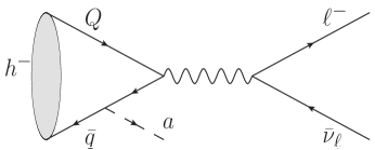
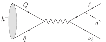
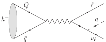
Figure 2: Feynman diagrams of $h\rightarrow\ell\bar{\nu}_{\ell}a$. $(a)$, $(b)$ , $(c)$ and $(d)$ represent the ALP couples with the quark, antiquark, charged lepton and antineutrino, respectively.

The Feynman amplitude corresponding to each diagram can be written by using the meson wave function. Here, as we are considering the heavy flavored meson, which can be seen as a two-body bound state including at least one heavy quark (or antiquark), the instantaneous BS wave function is appropriate for the calculation. This kind of wave functions have been extensively used to study the decay processes of heavy mesons. For the pseudoscalar meson, its wave function has the form Kim and Wang (2004)

$$\varphi\left(q_{\perp}\right)=M\left[\frac{\not{P}}{M}f_{1}(q_{\perp})+f_{2}(q_{\perp})+\frac{\not{q}_{\perp}}{M}f_{3}(q_{\perp})+\frac{\not{P}\not{q}_{\perp}}{M^{2}}f_{4}(q_{\perp})\right]\gamma^{5},$$ (3)

where $P$ is the meson momentum, and $q$ is the relative momentum between the quark and antiquark; $q^{\mu}_{\perp}\equiv q^{\mu}-\frac{P\cdot q}{M^{2}}P^{\mu}=(0,~{}\vec{q})$; $f_{i}$ is the radial wave function which can be achieved by solving the eigenvalue equations numerically (e.g. the detailed results for $B_{c}$ meson can be found in Ref. Wang et al. (2022)).

The amplitude corresponding to Fig. 2(a) can be written as

$$\mathcal{M}_{a} =-i\frac{G_{F}}{\sqrt{2}}\frac{c_{Q}m_{Q}}{f_{\text{a}}}V_{qQ}\sqrt{N_{c}}\int\frac{d^{3}q_{\perp}}{{\left(2\pi\right)}^{3}}\text{Tr}\left[\gamma_{\mu}\left(1-\gamma^{5}\right)\frac{1}{\not{p}_{Q}-\not{k}_{a}-m_{Q}}\gamma^{5}\varphi\left(q_{\perp}\right)\right]$$ (4)

$$\times\bar{u}_{\ell}(k_{\ell})\gamma^{\mu}\left(1-\gamma^{5}\right)v_{\bar{\nu}}(k_{\bar{\nu}}),$$

where $c_{Q}$ is coupling constant; $m_{Q}$ is the mass of quark Q; $N_{c}=3$ is the color factor; $k_{a}$, $k_{\ell}$, and $k_{\bar{\nu}}$ are the momenta of ALP, charged lepton, and antineutrino, respectively; $p_{Q}$ is the momentum of quark Q, which is related to $P$ and $q$ as $p_{Q}=\frac{m_{Q}}{m_{Q}+m_{q}}P+q$ with $m_{q}$ being the mass of the antiquark. To get Eq. (4), we have made an approximation, namely $p_{Q}\approx\frac{m_{Q}}{m_{Q}+m_{q}}P+q_{\perp}$, so that the denominator is independent of the time component of the relative momentum $q$. After integrating out $q_{\perp}$, $\mathcal{M}_{a}$ becomes

$$\begin{split}\mathcal{M}_{a}=-iA_{Q}\left(F_{1}P^{\mu}+F_{2}k_{a}^{\mu}\right)\bar{u}_{\ell}(k_{\ell})\gamma^{\mu}\left(1-\gamma^{5}\right)v_{\bar{\nu}}(k_{\bar{\nu}}),\end{split}$$ (5)

where we have used $A_{Q}=\frac{c_{Q}m_{Q}G_{F}V_{qQ}}{f_{a}\sqrt{2}}$ for short; $F_{1}$ and $F_{2}$ are the form factors of the hadronic transition matrix element, which are functions of the squared momentum transition $(P-k_{a})^{2}$.

Similarly, the Feynman amplitude corresponding to Fig. 2(b) can be written as

$$\mathcal{M}_{b} =i\frac{G_{F}}{\sqrt{2}}\frac{c_{q}m_{q}}{f_{a}}V_{qQ}\sqrt{N_{c}}\int\frac{d^{3}q_{\perp}}{{\left(2\pi\right)}^{3}}\text{Tr}\left[\gamma_{5}\frac{1}{\not{p}_{q}-\not{k}_{a}+m_{q}}\gamma^{\mu}\left(1-\gamma^{5}\right)\varphi\left(q_{\perp}\right)\right]$$ (6)

$$\times\bar{u}_{\ell}(k_{\ell})\gamma_{\mu}\left(1-\gamma^{5}\right)v_{\bar{\nu}}(k_{\bar{\nu}}),$$

where $c_{q}$ is the coupling constant; $m_{q}$ and $p_{q}$ are the mass and momentum of the antiquark, respectively; $p_{q}$ has the form $p_{q}\approx\frac{m_{q}}{m_{Q}+m_{q}}P-q_{\perp}$. After integrating out $q_{\perp}$, we get

$$\mathcal{M}_{b}=iA_{q}(G_{1}P^{\mu}+G_{2}k^{\mu})\bar{u}_{\ell}(k_{\ell})\gamma_{\mu}\left(1-\gamma^{5}\right)v_{\bar{\nu}}(k_{\bar{\nu}}),$$ (7)

where $A_{q}=\frac{c_{q}m_{q}G_{F}V_{qQ}}{f_{a}\sqrt{2}}$; $G_{1}$ and $G_{2}$ are form factors.

When calculating the integral, one must be careful, since as the relative momentum $\vec{q}$ changes, the denominator of the propagator may be zero, which will lead to a nonvanishing imaginary part of the form factors. Specifically, we can write the propagator as

$$\begin{split}\frac{\text{1}}{\not{p}_{Q/q}-\not{k}_{a}+m_{Q/q}-i\epsilon}=\frac{\not{p}_{Q/q}-\not{k}_{a}-m_{Q/q}}{a+b\cos\theta+i\epsilon},\end{split}$$ (8)

where $\theta$ is the angle between $\vec{q}$ and $\vec{k}_{a}$. $a$ and $b$ are expressed as

$$\begin{split}&a=\left(\frac{m_{Q/q}}{m_{Q}+m_{q}}M-E_{a}\right)^{2}-m_{Q/q}^{2}-\vec{q}^{2}-\vec{k}_{a}^{2},\\ &b=\pm 2|\vec{q}||\vec{k}|,\end{split}$$

where $E_{a}$ is the energy of the ALP. We will first integrate out $\cos\theta$ analytically, and then integrate out $|\vec{q}|$ numerically. As $\vec{q}$ changes, $a+b$ and $a-b$ may have opposite signs, which means with a specific value of $\theta$ the pole can exist.

The Feynman amplitude corresponding to Fig. 2(c) can be written as

$$\begin{split}\mathcal{M}_{c}&=-i\frac{G_{F}}{\sqrt{2}}\frac{c_{\ell}m_{\ell}}{f_{a}}V_{qQ}\sqrt{N_{c}}\int\frac{d^{3}q_{\bot}}{{\left(2\pi\right)}^{3}}\text{Tr}\left[\gamma^{\mu}\left(1-\gamma^{5}\right)\varphi\left(q_{\perp}\right)\right]\\ &\times\bar{u}_{\ell}(k_{\ell})\gamma_{5}\frac{1}{\not{k}_{\ell}+\not{k}_{a}-m_{\ell}}\gamma_{\mu}\left(1-\gamma^{5}\right)v_{\bar{\nu}}(k_{\bar{\nu}}).\end{split}$$ (9)

where $c_{\ell}$ is the coupling constant. The hadronic part of the amplitude is proportional to the meson momentum Cvetic et al. (2004), with the proportionality being the decay constant $f_{h}$

$$\sqrt{N_{c}}\int\frac{d^{3}q_{\perp}}{(2\pi)^{3}}\mathrm{Tr}\left[\gamma^{\mu}\left(1-\gamma_{5}\right)\varphi(q_{\perp})\right]=f_{h}P^{\mu}.$$ (10)

Using Eq. (10) and defining $A_{\ell}=\frac{c_{\ell}m_{\ell}G_{F}V_{qQ}}{f_{a}\sqrt{2}}$ for short, $\mathcal{M}_{c}$ is simplified as

$$\begin{split}\mathcal{M}_{c}=-iA_{\ell}f_{h}\bar{u}_{\ell}(k_{\ell})\gamma_{5}\frac{\not{p}_{\ell}+\not{k}_{a}+m_{\ell}}{m^{2}_{a}+2p_{\ell}\cdot k}\not{P}\left(1-\gamma^{5}\right)v_{\bar{\nu}}(k_{\bar{\nu}}).\end{split}$$ (11)

The total Feynman amplitude is $\mathcal{M}=\mathcal{M}_{a}+\mathcal{M}_{b}+\mathcal{M}_{c}$. And the partial width of such a decay channel is achieved by finishing the three-body phase space integral

$$\Gamma=\frac{1}{64\pi^{3}M}\int_{m_{\ell}}^{E_{\ell max}}dE_{\ell}\int_{E_{\bar{\nu}min}(E_{\ell})}^{E_{\bar{\nu}max}(E_{\ell})}dE_{\bar{\nu}}\overline{|\mathcal{M}|^{2}},$$ (12)

where the upper and lower limits have the following forms

$$E_{\ell max} =\sqrt{\left(\frac{M^{2}+m_{\ell}^{2}-m_{a}^{2}}{2M}\right)^{2}-m_{\ell}^{2}},$$

$$E_{\bar{\nu}max/min}(E_{\ell}) =\frac{M^{2}-2ME_{\ell}+m_{\ell}^{2}-m_{a}^{2}}{2(M-E_{\ell}\mp\sqrt{E_{\ell}^{2}-m_{\ell}^{2}})}.$$

III Numerical Results

In this section, we will first use the formulas obtained above to calculate the limits of the coupling constants, and then the results will be applied to investigate the similar decays of the $B_{c}$ meson. We will focus on three different scenarios: first, the ALP couples only with a single fermion, namely the quark, the antiquark, or the charged lepton; second, the ALP couples with quarks and antiquarks, but not with leptons; third, the ALP couples with all the charged fermions with the same coupling constant.

During the calculation process, the following numerical values of three groups of physical quantities are adopted. (1) The masses of constituent quarks are from Ref. Li et al. (2017): $m_{u}=0.305$ GeV, $m_{d}=0.311$ GeV, $m_{s}=0.5$ GeV, $m_{c}=1.62$ GeV, and $m_{b}=4.96$ GeV. (2) The relevant CKM matrix elements are from Particle Data Group (PDG) Workman et al. (2022): $|V_{ub}|=3.82\times 10^{-3}$, $|V_{cd}|=0.211$, $|V_{cs}|=0.975$, and $|V_{cb}|=41.1\times 10^{-3}$. (3) The decay constant of $D$, $D_{s}$, and $B$ mesons are the Lattice QCD results Aoki et al. (2022): $f_{D}=212.6$ MeV, $f_{D_{s}}=249.9$ MeV, and $f_{B}=188$ MeV.

III.1 Scenario 1

We consider separately the coupling between the ALP and each charged fermion. For example, by setting $c_{q}$ and $c_{\ell}$ to zero, we get the branching fraction of $h^{-}\to\ell^{-}\bar{\nu}a$ with $c_{Q}/f_{a}$ and $m_{a}$ being unknown parameters. Then using the experimental results in Table I, we get the upper limits of $c_{Q}/f_{a}$ as functions of $m_{a}$. The same is true for the other two cases. The results are shown in Fig. 3. One notices that the curves raise rapidly when $m_{a}$ is large enough, which is mainly because the decreasing of phase space. The most stringent upper limits for different coupling constants come from different decay channels. For example, Fig. 3(a) shows that the most strict constraints of $c_{b}/f_{a}$ and $c_{c}/f_{a}$, which are of the order of $10^{2}~{}{\rm TeV}^{-1}$ when $m_{a}$ is less than $1$ GeV, come from $B^{-}\to\mu^{-}\bar{\nu}_{\mu}a$ and $D_{s}^{+}\to e^{+}\nu_{e}a$, respectively. One can also notice that the upper limit of $c_{e}/f_{a}$ in Fig. 3(c) is much higher than those of $c_{Q(q)}/f_{a}$ set up by the same channels, which is because of the small $m_{e}$.

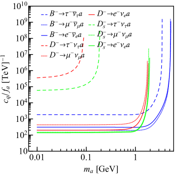
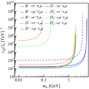
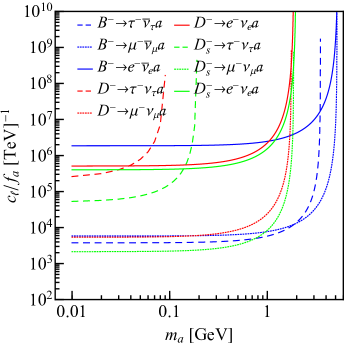
Figure 3: The upper limits of the coupling constants (a) $c_{Q}/f_{a}$ , (b) $c_{q}/f_{a}$ and (c) $c_{\ell}/f_{a}$ derived from the leptonic decays of $D$, $D_{s}$, and $B$ mesons.

Using above results, we can impose restrictions on $\mathcal{B}(B_{c}^{-}\to\ell^{-}\bar{\nu}_{\ell}a)$, which are presented in Fig. 4. We can see that when $m_{a}$ is less than 1 GeV, the branching ratios upper limits for ALP-quark coupling cases are of the order of $10^{-4}$, while for the ALP-tau coupling case, the order of magnitudes is $10^{-2}$, which is much larger than those of the ALP-$e/\mu$ coupling cases. We also notice that all the curves, except the one corresponding to $B_{c}^{-}\to\tau^{-}\bar{\nu}_{\tau}a$ in Fig. 4(a), show an ascending trend. This is because the maximum value of $m_{a}$ permitted in the $B_{c}$ decay is larger than that in the same decays of $B$ and $D_{(s)}$ mesons. For example, when we use $c_{b}/f_{a}$ from $B^{-}\to\mu^{-}\bar{\nu}_{\mu}a$ to constrain the branching ratios of $B_{c}^{-}\to\mu^{-}\bar{\nu}_{\mu}a$, the result blows up before $m_{a}$ reaches its maximum. The appearance of kinks in Fig. 4(c) is because we have used $c_{e/\mu}/f_{a}$ from different channels when $m_{a}$ takes different values.

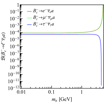
(a)  ALP couples with $b$ quark

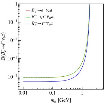
(b)  ALP couples with $c$ quark

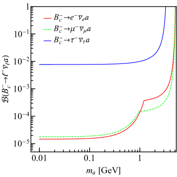
(c)  ALP couples with $\ell^{-}$

Figure 4: The upper limits of $\mathcal{B}(B_{c}^{-}\to\ell^{-}\bar{\nu}_{\ell}a)$ in scenario 1.

III.2 Scenario 2

In this scenario, we consider the case that the ALP couples with quarks but not with leptons. Two assumptions are made. First, all the coupling constants are assumed to be real numbers, and no additional relative phase is introduced. Second, the coupling constants of the ALP and light quarks, denoted by $c_{q}$, are assumed to be equal, while for those of heavy quarks, $c_{Q}$ ($Q=c,~{}b$) may have different values. We let $c_{q}$ be a free parameter, then use the experimental results of $B$ and $D_{(s)}$ mesons to provide constraints on $c_{b}$ and $c_{c}$. Specifically, we first write the following expression,

$$\delta\Gamma \equiv\Gamma(h^{-}\to\ell^{-}\not{E})-\Gamma(h^{-}\to\ell^{-}\bar{\nu}_{\ell})$$ (13)

$$\geq\Gamma(h^{-}\to\ell^{-}\bar{\nu}_{\ell}a)=\frac{c^{2}_{Q}}{f_{a}^{2}}\tilde{\Gamma}_{Q}+\frac{c^{2}_{q}}{f_{a}^{2}}\tilde{\Gamma}_{q}+\frac{c_{Q}c_{q}}{f_{a}^{2}}\tilde{\Gamma}_{Qq},$$

where the three terms on the right side of the last equation represent the contributions of Fig. 2(a), 2(b) and their interference, respectively; $\tilde{\Gamma}$ denotes the decay width devided by the coupling constant sqaured, which can be calculated theoretically.

The experimental allowed region for $c_{Q}$ and $c_{q}$ is determined by Eq. (13). We investigate all the decay channels, and find that the decays of $B^{-}$ and $D^{-}$ mesons give the most stringent constraint. The area of the parameter space depends on $m_{a}$. In Fig. 5, as two examples, we show the results when $m_{a}$=0, and 1.6 GeV, respectively.

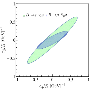
(a)  $m_{a}=0$ GeV

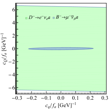
(b)  $m_{a}=1.6$ GeV

Figure 5: The experimental allowed region (inside the ellipse) of the coupling constants. The green and blue areas correspond to $Q=c$ and $Q=b$, respectively.

One can see that when $m=0$ GeV, the two areas are comparable, while when $m=1.6$ GeV, the area for $Q=c$ (just partially plotted) is more larger than that of $Q=b$.

Next, we scan the experimental allowed parameter area in Fig. 5, and calculate the limits of $\mathcal{B}(B_{c}^{-}\to\ell^{-}\bar{\nu}_{\ell}a)$. Because both $c_{Q}$ and $c_{q}$ changing the sign does not affect the results, we only need to consider the region with $c_{q}\geq 0$. Our strategy is as follows. First, by solving Eq. (13), we obtain the boundary values of $c_{Q}$ for a fixed $c_{q}$,

$$\begin{split}C_{Q(max)}&=\frac{-C_{q}\tilde{\Gamma}_{Qq}+\sqrt{(C_{q}\tilde{\Gamma}_{Qq})^{2}-4\tilde{\Gamma}_{Q}(C_{q}^{2}\tilde{\Gamma}_{q}-\delta\Gamma)}}{2\tilde{\Gamma}_{Q}},\\ C_{Q(min)}&=\frac{-C_{q}\tilde{\Gamma}_{Qq}-\sqrt{(C_{q}\tilde{\Gamma}_{Qq})^{2}-4\tilde{\Gamma}_{Q}(C_{q}^{2}\tilde{\Gamma}_{q}-\delta\Gamma)}}{2\tilde{\Gamma}_{Q}},\end{split}$$ (14)

where we have defined $C_{Q(q)}=c_{Q(q)}/f_{a}$. The condition $C_{q}^{2}\leq\frac{4\tilde{\Gamma}_{Q}\delta\Gamma}{4\tilde{\Gamma}_{Q}\tilde{\Gamma}_{q}-\tilde{\Gamma}_{Qq}^{2}}$ should be satisfied to make sure the quantity under the square root nonnegative. Second, we scan $C_{b}$ and $C_{c}$ together for a fixed $C_{q}$ whose allowed region is determined by the small ellipse in Fig. 5.

Finally, we calculate the upper limits of $\mathcal{B}(B_{c}^{-}\to\ell^{-}\bar{\nu}_{\ell}a)$ as functions of $C_{q}$ with a specific $m_{a}$. The results are shown in Fig. 6(a) and (c). Here we only present the result for the positive $C_{q}$, and that of the negative $C_{q}$ is symmetrical with it about the vertical axis. It can be seen that as $m_{a}$ increases, the experimental allowed region of $C_{q}$ shrinks, and the upper limit of $\mathcal{B}(B_{c}^{-}\to\ell^{-}\bar{\nu}_{\ell}a)$ roughly increases with $m_{a}$. This can be understood from Fig. (5), where as $m_{a}$ changes from 0 GeV to 1.6 GeV, the allowed range of $c_{c}/f_{a}$ becomes quite large, which leads to a larger upper limit. The interesting thing is that for some range of $c_{q}$, there is also a nonvanishing lower limit of the branching fraction (see Fig. 6(b) and (d)). From Fig. 5 we can see the two ellipses are tilted, so at some $c_{q}$, $c_{b}$ and $c_{c}$ cannot be zero at the same time, which leads to the nonvanishing $\mathcal{B}(B_{c}^{-}\to\ell^{-}\bar{\nu}_{\ell}a)$.

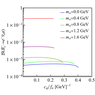
(a)  upper limit with $\ell=e$

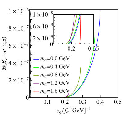
(b)  lower limit with $\ell=e$

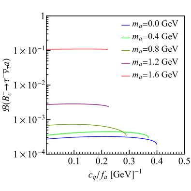
(c)  upper limit with $\ell=\tau$

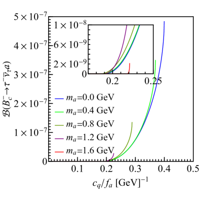
(d)  lower limit with $\ell=\tau$

Figure 6: The upper and lower limits of $\mathcal{B}(B_{c}\rightarrow\ell\bar{\nu}_{\ell}a)$ in scenario 2.

III.3 Scenario 3

In this scenario, we assume that the ALP couples with all the charged fermions with the same coupling constant $c_{q}=c_{Q}=c_{l}=c$, the upper limits of which as functions of $m_{a}$ are shown in Fig. 7(a). We can see the $B^{-}\to\mu\bar{\nu}_{\mu}a$ channel gives the most stringent restriction. We also notice that the curves have undulation around 1 GeV. To see why this happened, we take the $B^{-}\to\mu\bar{\nu}_{\mu}a$ channel as an example, and plot the contributions of three Feynman diagrams in Fig. 2 and the corresponding interference terms. It can be seen that the effect of the lepton can be neglected because of its small mass, while the coupling between the ALP and quarks provides the main contribution, especially the interference term, which has sizable negative value when $m_{a}<2$ GeV. This causes the total result to be undulant around $m_{a}=1$ GeV, which is also transferred to the coupling constant.

Using the upper limit of the coupling constant given by the $B^{-}\to\mu\bar{\nu}_{\mu}a$ channel, we obtain the constraints of the branching fraction of $B_{c}^{-}\to\ell^{-}\bar{\nu}_{\ell}a$, which are shown in Fig. 8(a). We can see, for $\mathcal{B}(B_{c}^{-}\to e^{-}\bar{\nu}_{e}a)$ and $\mathcal{B}(B_{c}^{-}\to\mu^{-}\bar{\nu}_{\mu}a)$, the upper limit is about $10^{-6}$ when $m_{a}$ is less than 1 GeV, and then it keeps increasing until being larger than one. The reason for this is that the phase space of the $B$ decay is small compared with that of the $B_{c}^{-}$ decay when $\ell=e$ or $\mu$. For $\mathcal{B}(B_{c}^{-}\to\tau^{-}\bar{\nu}_{e}a)$, the upper limit is around $10^{-5}$ when $m_{a}<1$ GeV, and then there is a fluctuation with the peak value of $5.4\times 10^{-4}$ at $m_{a}=3.4$ GeV, and finally the branching fraction goes to zero because of the vanishing phase space. It is worth to compare these results with the branching fractions of $B_{c}^{-}\to\ell^{-}\bar{\nu}_{\ell}$ in SM. Using Eq. (1) and (10) we get $\mathcal{B}(B_{c}^{-}\to\ell\bar{\nu}_{\ell})=2.2\times 10^{-9},~{}9.5\times 10^{-5}$, and $2.2\times 10^{-2}$ for $\ell=e,~{}\mu$, and $\tau$, respectively. One can see that $\mathcal{B}(B_{c}^{-}\to e^{-}\bar{\nu}_{e})$ is much smaller than the upper limit of $\mathcal{B}(B_{c}^{-}\to e^{-}\bar{\nu}_{e}a)$ for the chiral suppression; on the contrary, $\mathcal{B}(B_{c}^{-}\to\tau^{-}\bar{\nu}_{\tau})$ is much larger than the upper limit of $\mathcal{B}(B_{c}^{-}\to\tau^{-}\bar{\nu}_{\tau}a)$.

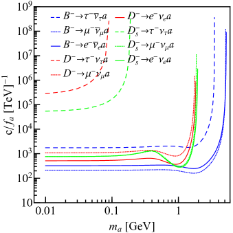
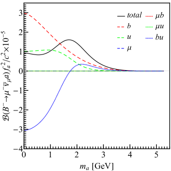
Figure 7: (a) shows the upper limits of the coupling constants in scenario 3. (b) shows the contributions to $\mathcal{B}(B^{-}\to e^{-}\bar{\nu}_{e}a)f_{a}^{2}/c_{i}^{2}$ by each Feynman diagram and the interference terms.

In Fig. 8(b), (c), and (d), we present the upper limits of the differential branching fractions as functions of the lepton energy. For $\ell$ being $e$ or $\mu$, the results are similar because of the small lepton mass, while for $\ell=\tau$, the distribution shape is quite different. We can see that as $m_{a}$ gets larger, the peak moves left. Experimentally, the detection of the unmonoenergetic charged lepton in the decay $h^{-}\to\ell^{-}\not{E}$ may indicate the existence of ALP. Around the peak, it has the largest experimental allowed probability to find the charged lepton.

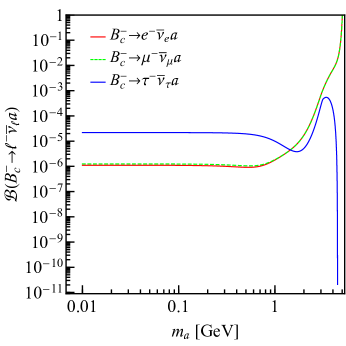
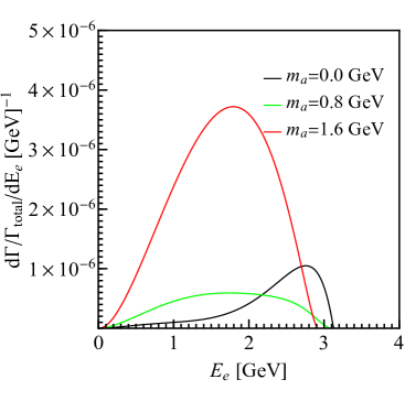
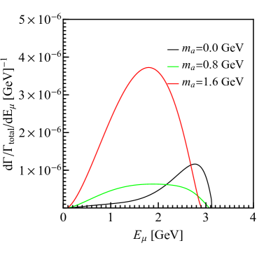
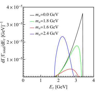
Figure 8: (a) shows the upper limit of $\mathcal{B}(B_{c}^{-}\to\ell^{-}\bar{\nu}_{\ell}a)$ in scenario 3. (b), (c), and (d) shows the upper limits of the differential branching fraction with $\ell=e$, $\mu$, and $\tau$, respectively.

IV Summary

To conclude, we have studied the ALP production through the processes $h^{-}\to\ell^{-}\bar{\nu}_{\ell}a$. The instantaneous BS wave functions of the heavy mesons are applied to compute the branching fractions of such decay channels. We adopt three scenarios, that is the ALP coupling only to one charged fermion, the ALP coupling only to quarks, and the ALP coupling to all the charged fermions with the same coupling constant. In each scenario, by comparing the theoretical and experimental results, we get the upper limits of the coupling constants, which are then used to calculate the upper limits of the branching fractions of the $B_{c}^{-}\to\ell^{-}\bar{\nu}_{\ell}a$ channel. For the second scenario, we also get the nonzero lower limit of the branching fraction at some range of $c_{q}$. We hope this work could be helpful for the future detection of the ALP through heavy meson decays.