Efficient Bayesian dynamic closed skew-normal model preserving mean and covariance for spatio-temporal data

Abstract

Although Bayesian skew-normal models are useful for flexibly modeling spatio-temporal processes, they still have difficulty in computation cost and interpretability in their mean and variance parameters, including regression coefficients. To address these problems, this study proposes a spatio-temporal model that incorporates skewness while maintaining mean and variance, by applying the flexible subclass of the closed skew-normal distribution. An efficient sampling method is introduced, leveraging the autoregressive representation of the model. Additionally, the model’s symmetry concerning spatial order is demonstrated, and Mardia’s skewness and kurtosis are derived, showing independence from the mean and variance. Simulation studies compare the estimation performance of the proposed model with that of the Gaussian model. The result confirms its superiority in high skewness and low observation noise scenarios. The identification of Cobb-Douglas production functions across US states is examined as an application to real data, revealing that the proposed model excels in both goodness-of-fit and predictive performance.

[label1] organization=The Graduate University for Advanced Studies,addressline=Shonan Village, city=Hayama, postcode=240-0193, state=Kanagawa, country=Japan

[label2] organization=BrainPad inc.,addressline=3-1-1 Roppongi, city=Minato-ku, postcode=108-0071, state=Tokyo, country=Japan

[label3] organization=Institute of Statistical Mathematics,addressline=10-3 Midori-cho, city=Tachikawa, postcode=190-8562, state=Tokyo, country=Japan

Developed a skew spatio-temporal model while preserving mean and covariance

Introduced efficient Bayesian inference via autoregressive model representation

Proved spatial symmetry and derived Mardia’s skewness and kurtosis

Outperformed the Gaussian model in scenario with high skewness and low noise

Excelled in fit and prediction over the Gaussian model for real data applications

1 Introduction

An increasing variety of spatial and spatio-temporal data are becoming available owing to the development of sensing and positioning technologies. Alongside this, spatial statistical models have been developed to describe spatio-temporal processes underlying potentially noisy observations. These models are applied in various fields, including disease mapping (e.g., Best et al., 2005), species distribution modeling (e.g., Dormann et al., 2007), and socio-econometric analysis (e.g., Anselin, 2022).

It is common to assume that the spatio-temporal process follows a Gaussian distribution, with its covariance parameterized to model spatial correlations. Conditional autoregressive (CAR) and Gaussian process models are among such specifications (see Gelfand et al., 2010). With this Gaussian assumption, the posterior mean and variance of the spatio-temporal process are available in closed form; this property greatly simplifies the resulting inference and prediction. However, Gaussianity may not hold in many real-world cases (Tagle et al., 2019). Consequently, there has been growing interest in developing models that can represent spatio-temporal structures accommodating skewness (Schmidt et al., 2017; Tagle et al., 2019).

Among the wide variety of non-Gaussian spatial processes (see Yan et al., 2020, for review), the skew-normal process (Kim and Mallick, 2004) is a straightforward extension that combines the Gaussian process and the skew-normal distribution (Azzalini, 1985; Azzalini and Capitanio, 1999). Allard and Naveau (2007) developed another skewed process based on a closed skew-normal (CSN) distribution, which is a variant of the skew-normal distribution. However, both skew-normal and CSN distributions suffer from an over-parameterization, leading to an identification problem (Arellano-Valle and Azzalini, 2006). Genton and Zhang (2012) suggested a similar problem in the context of spatial modeling. Although Arellano-Valle and Azzalini (2006) proposed the unified skew normal (SUN) distribution to unify several types of skew-normal distributions and address the identification problem, it is still non-identifiable in some cases (Wang et al., 2023).

To ensure identifiability, skew-normal processes have been simplified. Márquez-Urbina and González-Farías (2022) proposed a flexible subclass of the CSN (FS-CSN) that makes the CSN identifiable, while Wang et al. (2023) proposed several sub-classes that make the SUN identifiable. Interestingly, FS-CSN coincides with one of these SUN’s sub-classes. FS-CSN is distinctive among alternatives in that it accounts for skewness while preserving mean and variance. In other words, the first two moments represent the mean and variance of the target variables, just like the Gaussian process models (Márquez-Urbina and González-Farías, 2022; Khaledi et al., 2023). This property greatly improves the interpretability of model parameters. For example, if the mean is specified by a regression function, the coefficients can be interpreted in the same manner as in a conventional Gaussian regression model. The variance, the strength of the spatial dependence, and other parameters are also directly interpretable. Such a interpretability does not hold for most skew-normal regression models (Márquez-Urbina and González-Farías, 2022).

Still, FS-CSN faces difficulties in terms of spatio-temporal modeling. First, to the best of the author’s knowledge, temporal dynamics have never been introduced; it is unclear how to apply FS-CSN to spatio-temporal data. Second, despite Bayesian inference is commonly used for in modern spatio-temporal statistics, fully Bayesian estimation has never been tackled for FS-CSN models. In addition, the Bayesian inference for the spatio-temporal FS-CSN model is computationally demanding, which constitutes the third difficulty.

Building upon these considerations, this study proposes a spatio-temporal FS-CSN model that incorporates skewness while preserving mean and variance. Subsequently, we develop an efficient Bayesian estimation method for this model.

The structure of this paper is as follows. In Section 2, we describe the dynamic CAR model, a conventional spatio-temporal model, and the FS-CSN model, a multivariate spatial model capable of handling skewness while preserving mean and variance. Then, in Section 3, we extend the FS-CSN model to the spatio-temporal model and develop the efficient estimation method. In Section 4, we investigate the inverse estimation performance of this model, particularly comparing it with models ignoring skewness. In Section 5, the proposed model is applied to identify the Cobb-Douglas production functions for each state in the United States, again comparing it with the performance of the conventional model.

2 Preliminaries

2.1 Dynamic CAR model

In this paper, we primarily consider extensions that incorporate skewness into a dynamic CAR (D-CAR) model (Lee et al., 2018). The model follows a first-order autoregressive (AR) model in the temporal dimension and a CAR model in the spatial dimension. It is formulated as follows:

$$\theta_{t} =\rho_{T}\theta_{t-1}+w_{t},\ w_{t}\sim N_{K}(0_{K},\Omega),$$ (1)

$$y_{t} =X_{t}\beta+\theta_{t}+v_{t},\ v_{t}\sim N_{K}(0_{K},\sigma^{2}I_{K}),$$ (2)

where $t=1,\ldots,T$, $\rho_{T}\in\mathbb{R}$, $\theta_{t}\in\mathbb{R}^{K}$, $y_{t}\in\mathbb{R}^{K}$, $X_{t}\in\mathbb{R}^{K\times r}$, $0_{K}=(0,\ldots,0)^{\prime}\in\mathbb{R}^{K}$, $I_{K}$ is a $K$-dimensional identity matrix, $K$ is the number of areas, $T$ is time length, and $r$ is the dimension of features. $\Omega$ is specified to describe spatial dependence, based on the Leroux model, the BYM model, or any other suitable model (see Gelfand et al., 2010). In the case of the Leroux model, the covariance matrix is given by:

$$\Omega =\tau^{2}Q^{-1},$$

$$Q =\rho_{S}({\rm diag}(W1_{K})-W)+(1-\rho_{S})I_{K},$$

where $\rho_{T}\in\mathbb{R}$, $\tau^{2}\in\mathbb{R}^{+}$, $1_{K}=(1,\ldots,1)^{\prime}\in\mathbb{R}^{K}$, and $W$ is an adjacency matrix with zero diagonals. In the D-CAR model, the distribution of $\theta_{1:T}=(\theta_{1}^{\prime},\ldots,\theta_{T}^{\prime})^{\prime}$ is expressed as follows:

$$\theta_{1:T}\sim\mathrm{N}_{TK}\left(0_{TK},R\otimes\Omega\right),$$ (3)

where $\otimes$ denotes a Kroneker product. Let $R_{t_{1},t_{2}}$ be the element in the $t_{1}$th row and $t_{2}$th column of $R$,

$$R_{t,t}=\sum_{i=1}^{t}\rho_{T}^{2(i-1)}, \text{ for }t=1,\ldots,T,$$

$$R_{t_{1},t_{2}}=R_{t_{2},t_{1}}=\rho_{T}^{t_{2}-t_{1}}\sum_{i=1}^{t_{1}}\rho_{T}^{2(i-1)}, \text{ for }1\leq t_{1}<t_{2}\leq T.$$

2.2 CSN and FS-CSN distribution

CSN is an extension of the normal distribution that incorporates skewness. Its probability density function, denoted by $\textrm{CSN}_{p,q}(\mu,\Sigma,D,\nu,\Delta)$, is expressed as follows:

$$f(z)=\phi_{p}(z;\mu,\Sigma)\frac{\Phi_{q}(D(z-\mu);\nu,\Delta)}{\Phi_{q}\left(0;\nu,\Delta+D\Sigma D^{\prime}\right)},$$

where $\mu\in\mathbb{R}^{p},\nu\in\mathbb{R}^{q},D\in\mathbb{R}^{q\times p}$, $\Sigma$ is a $p\times p$ covariance matrix, $\Delta$ is a $q\times q$ covariance matrix, and $\phi_{p}(z;\mu,\Sigma)$ and $\Phi_{p}(z;\mu,\Sigma)$ are the probability distribution function and the cumulative distribution function of the $p$-dimensional normal distribution with mean vector $\mu$ and covariance matrix $\Sigma$.

Additionally, FS-CSN is a modified version of the CSN distribution that ensures the mean and variance remain consistent with those of a multivariate normal distribution, while also making parameters identifiable. When a random variable $z$ follows $\textrm{FS-CSN}_{p}(\mu,\Omega,\lambda,\Omega^{c})$, it means that $z$ adheres to the following distribution:

$$z\sim\textrm{CSN}_{p,p}\left(\mu-b\delta\gamma\Omega^{c}1_{p},\gamma^{2}\Omega,\frac{\lambda}{\gamma}\Omega^{-c},0_{p},I_{p}\right),$$ (4)

where $b=\sqrt{2/\pi}$, $\delta=\lambda/\sqrt{1+\lambda^{2}}$, $\gamma=1/\sqrt{1-b^{2}\delta^{2}}$, and $\Omega^{c}$ and $\Omega^{-c}$ are the Cholesky decomposition of $\Omega$ and its inverse, respectively. In Márquez-Urbina and González-Farías (2022), the variance is formulated as a constant multiple of the correlation matrix. However, in this paper, $\Omega$ is assumed to be the unconstrained covariance matrix for the purposes of subsequent discussions. Similarly, for the purposes of the following discussion, it is explicitly stated that matrix decomposition employs the Cholesky decomposition, with $\Omega^{c}$ being specifically delineated.

Figure 1 illustrates the probability density function of the $\textrm{FS-CSN}_{1}(0,1,\lambda,1)$ distribution for each $\lambda$. At $\lambda=0$, it coincides with the normal distribution, and as $\lambda$ increases, it approaches a half-normal distribution truncated at $-b\delta\gamma$, with a mean of $-b\delta\gamma$, converging to a half-normal distribution when $\lambda\rightarrow\infty$.

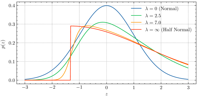
Figure 1: The probability density function of the FS-CSN distribution for each $\lambda$

3 Proposed method

3.1 Proposed model

As observed in equation (4), the original paper on FS-CSN considers Cholesky decomposition (Márquez-Urbina and González-Farías, 2022). However, if the sole objective is to maintain mean and variance, any decomposition that results in the product of the decomposed matrix and its transpose equating to the original matrix is acceptable. A quintessential example of such a decomposition is the matrix square root. Unlike FS-CSN that employs Cholesky decomposition, FS-CSN utilizing the matrix square root is symmetric under permutation, as we will see in the following proposition.

Proposition 3.1.

$\textrm{FS-CSN}_{p}(\mu,\Omega,\lambda,\Omega^{s})$ is symmetric under permutation, where $\Omega^{s}$ denotes the square root of $\Omega$. The proof is provided in the Appendix.

If the symmetry does not hold under permutation, a change in the order of the samples can alter the estimation results. Therefore, it is fundamentally preferable to use the square root of a matrix to decompose the spatial correlation matrix. However, as seen below, there are cases where use of Cholesky decomposition is advantageous, as well as scenarios where combining Cholesky decomposition and the square root of a matrix yields better results.

In this study, we propose the dynamic FS-CSN model (D-FS-CSN), which includes the D-CAR model as a subclass, to account for the skewness of $\theta_{1:T}$. This model adheres to the following distribution:

$$\theta_{1:T} \sim\textrm{FS-CSN}_{TK}(0_{TK},R\otimes\Omega,\lambda,R^{c}\otimes\Omega^{s}),$$ (5)

$$y_{1:T} \sim N_{TK}(X_{1:T}\beta+\theta_{1:T},\sigma^{2}I_{TK}),$$ (6)

where $X_{1:T}=(X_{1}^{\prime},\ldots,X_{T}^{\prime})^{\prime}$ and $y_{1:T}=(y_{1}^{\prime},\ldots,y_{T}^{\prime})^{\prime}$. Based on equation (3), (5) utilizes the square root of the spatial covariance matrix $\Omega$, and employs Cholesky decomposition for the temporal covariance matrix $R$. The matrix square root of $\Omega$ is used to ensure symmetry under permutation (see Proposition 3.1). On the other hand, the rationale for using Cholesky decomposition for $R$ is that equation (5) is naturally expressed as an AR model in that case, as demonstrated in the following proposition. Given the Cholesky decomposition for $R$ as assumed, the model is not symmetric with respect to permutations in the temporal direction. However, it does not pose a problem. This is explained by the fact that spatial adjacency is undirected, whereas temporal adjacency is directed.

Proposition 3.2.

The model represented by equations (5) and (6) is equivalent to the model expressed below:

$$\theta_{t} =\rho_{T}\theta_{t-1}+w_{t},\ w_{t}\sim\textrm{FS-CSN}_{K}(0,\Omega,\lambda,\Omega^{s}),$$

$$y_{t} =X_{t}\beta+\theta_{t}+v_{t},\ v_{t}\sim N_{K}(0,\sigma^{2}I_{K}),$$

where $\theta_{1}\sim\textrm{FS-CSN}_{K}(0,\Omega,\lambda,\Omega^{s})$. The proof is provided in the Appendix.

Conversely, this proposition demonstrates that by assuming the FS-CSN distribution for the noise term in the AR model, the joint distribution also becomes an FS-CSN distribution. The fact that the joint distribution is closed under the FS-CSN distribution means that the mean and variance coincide with those of the D-CAR model. Additionaly, this implies that $\theta_{1:T}$ has properties as demonstrated by Márquez-Urbina and González-Farías (2022).

While Márquez-Urbina and González-Farías (2022) derived properties of skewness and kurtosis in the univariate case, it is essential to consider these measures from a multivariate perspective. The multivariate equivalents of skewness and kurtosis are known as Mardia’s skewness $\mathrm{MS}(z)$ and kurtosis $\mathrm{MK}(z)$, respectively. For a multivariate variable $z$ with mean $\mu_{z}$ and covariance matix $\Sigma_{z}$, $\mathrm{MS}(z)$ and $\mathrm{MK}(z)$ follow the expressions given below.

$$\mathrm{MS}(z) =\mathbb{E}[((z-\mu_{z})^{\prime}\Sigma_{z}^{-1}(z-\mu_{z}))^{3}],$$

$$\mathrm{MK}(z) =\mathbb{E}[((z-\mu_{z})^{\prime}\Sigma_{z}^{-1}(z-\mu_{z}))^{2}].$$

Within the context of the FS-CSN and D-FS-CSN distributions, Mardia’s skewness and kurtosis exhibit the following properties:

Proposition 3.3.

When $z$ follows $\textrm{FS-CSN}_{p}(0_{p},\Omega,\lambda,\Omega^{1/2})$, Mardia’s skewness and kurtosis for $z$ are given by:

$$\mathrm{MS}(z) =pb^{2}(2b^{2}-1)^{2}\delta^{6}\gamma^{6},$$ (7)

$$\mathrm{MK}(z) =p\left(p+2+2b^{2}(2-3b^{2})\delta^{4}\gamma^{4}\right),$$ (8)

where $\Omega^{1/2}$ represents any matrix decomposition satisfying $\Omega=\Omega^{1/2}(\Omega^{1/2})^{\prime}$. Furthermore, when $\lambda=0$, $\mathrm{MS}(z)=0$ and $\mathrm{MK}(z)=p(p+2)$. Additionaly, the following properties naturally emerge.

$$\lim_{\lambda\rightarrow\infty}\mathrm{MS}(z) =p\left(\frac{b(2b^{2}-1)}{(1-b^{2})^{3/2}}\right)^{2},$$

$$\lim_{\lambda\rightarrow\infty}\mathrm{MK}(z) =p\left(p+2+\frac{2b^{2}(2-3b^{2})}{(1-b^{2})^{2}}\right).$$

The proof is provided in the Appendix.

From the above equation, it can be discerned that Mardia’s skewness and kurtosis of the FS-CSN distribution are determined solely by the dimension $p$ and $\lambda$. This implies that within the FS-CSN distribution, the mean, variance, and Mardia’s skewness can be independently specified. Moreover, the results of equation (7) are consistent with those of Márquez-Urbina and González-Farías (2022). Specifically, if the Mardia’s skewness of the $p$-dimensional random variables whose elements each follow an independent univariate FS-CSN distribution, according to Márquez-Urbina and González-Farías (2022), the value equals equation (7). Mardia’s skewness and kurtosis are $0$ and $p(p+2)$ for a $p$-dimensional normal distribution while they are $p\left(b(2b^{2}-1)/(1-b^{2})^{3/2})\right)^{2}$ and $p\left(p+2+2b^{2}(2-3b^{2})/(1-b^{2})^{2}\right)$ for $p$ independent half-normal distribution. Based on the skewness and kurtosis of the three distributions, it can be inferred that the FS-CSN distribution lies between the multivariate normal distribution and the multivariate half-normal distribution. This result is readily applicable to D-FS-CSN distribution; the Mardia’s skewness and kurtosis of $\theta_{1:T}$ under the D-FS-CSN distribution are determined by setting $p=TK$ in equations (7) and (8).

3.2 Sampling method from posterior distribution

Sampling from the posterior distribution under D-FS-CSN model presents a significant challenge, particularly when sampling from the posterior distribution of $\theta_{1:T}$. This posterior distribution of $\theta_{1:T}$ can be analytically expressed as a CSN distribution:

$$\theta_{1:T}|y_{1:T},\beta,\sigma^{2},\Omega,\rho_{T},\lambda$$

$$\qquad\sim\textrm{CSN}_{TK,TK}(\mu_{post},\Sigma_{post},D_{post},\nu_{post},\Delta_{post}),$$ (9)

$$\qquad\mu_{post}=\mu_{pre}+\Sigma_{pre}(\Sigma_{pre}+\sigma^{2}I_{TK})^{-1}(y_{1:T}-\mu_{pre}-X_{1:T}\beta),$$

$$\qquad\Sigma_{post}=\Sigma_{pre}-\Sigma_{pre}(\Sigma_{pre}+\sigma^{2}I_{TK})^{-1}\Sigma_{pre},$$

$$\qquad D_{post}=\sigma^{2}\lambda(\Sigma_{pre}^{1/2})^{\prime}(\Sigma_{pre}+\sigma^{2}I_{TK})^{-1}\Sigma_{post}^{-1},$$

$$\qquad\nu_{post}=\lambda\Sigma^{1/2}(\Sigma_{pre}+\sigma^{2}I_{TK})^{-1}(y_{1:T}-\mu_{pre}-X_{1:T}\beta),$$

$$\qquad\Delta_{post}=(1+\lambda^{2})I_{TK}-\lambda^{2}(\Sigma_{pre}+\sigma^{2}I_{TK})^{-1}\Sigma_{pre}-D_{post}\Sigma_{post}D_{post}^{\prime},$$

where $\mu_{pre}=-b\delta\Sigma_{pre}^{1/2}1_{TK}$, $\Sigma_{pre}=\gamma^{2}R\otimes\Omega$, and $\Sigma_{pre}^{1/2}=\gamma R^{c}\otimes\Omega^{s}$. While it is possible to sample using this formula, it requires computing the inverse of a $TK\times TK$ matrix and the sampling from a $TK$-dimensional multivariate truncated normal distribution. Sampling from such a distribution is computationally demanding (Botev, 2017).

Therefore, this study proposes an efficient sampling method utilizing data augmentation techniques and leveraging the representation of the AR model as demonstrated in Proposition 2.2. Initially, $\theta_{t}$ is decomposed into a sum of random variables as follows:

$$\theta_{t} \sim N_{K}\left(-b\delta\gamma\Omega^{s}1_{K}+\frac{\gamma\lambda}{1+\lambda^{2}}\Omega^{s}\alpha_{t},\frac{\gamma^{2}}{1+\lambda^{2}}\Omega\right),$$

$$\alpha_{t} \sim TN_{K}(0_{K},(1+\lambda^{2})I_{K}),$$

where $TN_{K}(\mu,\Sigma)$ denote $N_{K}(\mu,\Sigma)$ truncated below $0_{K}$. Consequently, we consider sampling $\theta_{t}$ and $\alpha_{t}$ separately. Regarding the posterior distribution of $\theta_{1:T}$, conditioned on $\alpha_{1:T}$, it becomes a normal distribution allowing the use of the forward filtering backward sampling (FFBS) method (Carter and Kohn, 1994; Frühwirth-Schnatter, 1994). The specific filtering approach can be described as follows. Let $\theta_{t_{1}|t_{2}}$ be $\theta_{t_{1}}|y_{1:t_{2}},\alpha_{1:T},\beta,\sigma^{2},\Omega,\rho_{T},\lambda$ with mean and covariace matrix of $\theta_{t_{1}|t_{2}}$ be $\mu_{t_{1}|t_{2}}$ and $\Sigma_{t_{1}|t_{2}}$, then

$$\mu_{t|t-1} =\rho_{T}\mu_{t-1|t-1}-b\delta\gamma\Omega^{s}1_{K}+\frac{\gamma\lambda}{1+\lambda^{2}}\Omega^{s}\alpha_{t},$$

$$\Sigma_{t|t-1} =\rho_{T}^{2}\Sigma_{t-1|t-1}+\frac{\gamma^{2}}{1+\lambda^{2}}\Omega,$$

$$\mu_{t|t} =\mu_{t|t-1}+\Sigma_{t|t-1}(\Sigma_{t|t-1}+\sigma^{2}I)^{-1}(y_{t}-X_{t}\beta-\mu_{t|t-1}),$$

$$\Sigma_{t|t} =\sigma^{2}\Sigma_{t|t-1}(\Sigma_{t|t-1}+\sigma^{2}I)^{-1},$$

where $\mu_{1|0}$ is $-b\delta\gamma\Omega^{s}1_{K}+\gamma\lambda/(1+\lambda^{2})\Omega^{s}\alpha_{1}$, and variance is $\Sigma_{1|0}=\gamma^{2}/(1+\lambda^{2})\Omega$. It is possible to calculate $p(\theta_{t}|y_{1:t},\alpha_{1:T},\beta,\sigma^{2},\Omega,\rho_{T},\lambda)$ iteratively for $t=1,\ldots,T$. $\theta_{t|T}$ can be sequentially sampled by iteratively using the following formula:

$$\mu_{t|T} =\mu_{t|t}+\rho_{T}\Sigma_{t|t}\Sigma_{t+1|t}^{-1}(\theta_{t+1|T}^{(i)}-\mu_{t+1|t}),$$

$$\Sigma_{t|T} =\Sigma_{t|t}-\Sigma_{t|t}\Sigma_{t+1|t}^{-1}\Sigma_{t|t},$$

where $\theta_{t+1|T}^{(i)}$ is a sample of $\theta_{t+1|T}$. Additionally, an important computational technique involves computing the eigenvalue matrix of $\Omega$ as $\rho_{S}E_{W}+(1-\rho_{S})I_{K}$, where $E_{W}$ is the eigendecomposition of the adjacency matrix $W$. By pre-computing the eigendecomposition $E_{W}$, the square root and inverse of $\Omega$ can be efficiently calculated. Next, $\alpha_{t}|\theta_{1:T},\Omega,\rho_{T},\lambda$ is distributed as $TN_{K}(\lambda/\gamma\Omega^{-s}(\theta_{t}-\rho_{T}\theta_{t-1}+b\delta\gamma\Omega^{s}1_{K}),I_{K})$, which is a multivariate truncated normal distribution with independent univariate truncated normal distributions in each dimension, simplifying the sampling process.

Sampling using the equation (9) requires a computational complexity of $O(T^{3}K^{3})$ both for calculating the inverse of a $TK\times TK$ matrix and for sampling from a $TK$-dimensional multivariate truncated normal distribution (Botev, 2017). In contrast, the sampling method described above only necessitates computing the inverse of a $K\times K$ matrix and sampling $\alpha_{t}$ from independently distributed truncated normal distributions, resulting in a computational complexity of $O(TK^{3})$. This is particularly efficient when $T$ is large.

Moreover, $p(\beta|y_{1:T},\theta_{1:T},\sigma^{2}),p(\sigma^{2}|y_{1:T},\theta_{1:T},\beta),p(\rho_{T}|\theta_{1:T},\tau^{2},\rho_{S})$ can be calculated analytically. However, the parameters of $\Omega$ cannot be sampled analytically. Therefore, the parameters of $\Omega$ are sampled using Metropolis-Hasting or Hamiltonian Monte Carlo. The overall workflow of the MCMC is detailed in the Appendix.

4 Simulation Studies

In the simulation study, the inverse estimation performance is investigated by inferring parameters from the results of simulating the D-FS-CSN model. Specifically, estimation is also conducted using a model that does not account for skewness, and changes in estimation accuracy are examined. In the following discussion, the model proposed in this paper, represented by equations (5) and (6), is referred to as the D-FS-CSN model, while the conventional model, represented by equations (1) and (2), is termed the D-CAR model.

Prior distributions are set as follows, based on Lee et al. (2018),

$$\beta \sim N_{r}(0,\sigma_{\beta}^{2}I),$$

$$\sigma^{2} \sim{\rm InverseGamma}(a_{\sigma^{2}},b_{\sigma^{2}}),$$

$$\tau^{2} \sim{\rm InverseGamma}(a_{\tau^{2}},b_{\tau^{2}}),$$

$$\rho_{S} \sim{\rm Uniform}(0,1),$$

$$\rho_{T} \sim{\rm Uniform}(0,1),$$

$$\lambda \sim N(0,\sigma_{\lambda}^{2}).$$

The prior distributions used for the D-CAR model are identical to those mentioned above, except for $\lambda$. In the simulation study, we set $\sigma^{2}_{\beta}=100$, $\alpha_{\sigma^{2}}=1$, $\beta_{\sigma^{2}}=0.01$, $\alpha_{\tau^{2}}=1$, $\beta_{\tau^{2}}=0.01$, and $\sigma^{2}_{\lambda}=9$. The time length is set to 10, and the location was represented by a $5\times 5$ grid. Furthermore, the adjacency matrix is defined by assigning 1 for the neighboring pairs sharing the border separating grids, and 0 for the other pairs.

In this simulation study, our primary interest lies in understanding how $\lambda$, the parameter determining skewness, affects the estimation results. Consequently, we conduct simulation studies under $\lambda$ values of $2.50$ and $7.00$, which are values previously used in Márquez-Urbina and González-Farías (2022). Additionally, since high observation noise $\sigma^{2}$ can obscure differences between the Normal model and others, we examine the changes in estimation accuracy under conditions of low and moderate observation noise. Since the strength of spatial correlation $\rho_{S}$ is crucial for evaluating estimation performance, we investigate three cases: $0.25$, $0.5$, and $0.75$. The simulation study organizes the parameters $\lambda$ and $\sigma^{2}$, $\rho_{S}$ for each case in Table 1. The true values for other parameters are set as follows: $\beta_{0}=1.00$, $\beta_{1}=0.50$, $\tau^{2}=1.00$ and $\rho_{T}=0.50$. For each case, simulation data were generated randomly 50 times, and 1,000 effective samples were drawn from the posterior distribution to evaluate the accuracy of parameter estimation.

Case	$\sigma^{2}$	$\lambda$	$\rho_{S}$
1	0.01	2.50	0.25
			0.50
			0.75
2	0.25	2.50	0.25
			0.50
			0.75
3	0.01	7.00	0.25
			0.50
			0.75
4	0.25	7.00	0.25
			0.50
			0.75

Table 1: Parameters for simulation studies

Figure 2 presents the differences in the root mean squared error (RMSE) between using the D-FS-CSN model and the D-CAR model, illustrated as box plots for each case. Overall, there is a trend towards improvement across all cases. However, the greatest improvement is observed in Case 3, while Case 2 exhibits the smallest improvement. This suggests that the effect of skewness becomes more pronounced with larger values of $\lambda$ and smaller values of $\sigma^{2}$. It was found that $\rho_{S}$, which determines the strength of spatial correlation, does not significantly impact the estimation accuracy.

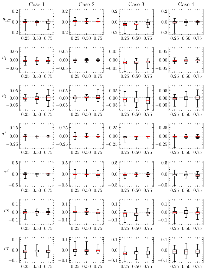
Figure 2: Difference of RMSE between D-FS-CSN and D-CAR for each case (x-axis denotes the values of $\rho_{S}$)

Simirarly, figure 3 displays the differences in predictive accuracy. Predictive accuracy is evaluated using log margianl predictive likelihood (LMPL), log margianl predictive likelihood in the future data (FLMPL), energy score in the future data (FES), and RMSE of $y$ in the future data (FRMSE). The calculation method for LMPL follows that used in the CarBayesST package (Lee et al., 2018). FLMPL is an estimator of LMPL for the future data $y_{T+1:T+T_{future}}$ conditioned on the learning data $y_{1:T}$, specifically $\log p(y_{T:T+T_{future}}|y_{1:T})$. Here, $T_{future}$ represents the length of the future data. FLMPL is calculated from samples of the posterior distribution as follows:

$$\mathrm{FLMPL}=\frac{1}{S}\sum_{i=1}^{S}\log p(y_{T+1:T+T_{future}}|\Theta^{(i)}),$$

where $\Theta^{(i)}$ is a sample of parameters from the posterior distribution conditioned on $y_{1:T}$ and $S$ is the number of samples. Energy Score is a generalization of the continuous ranked probability score, used to evaluate the accuracy of predictions for multivariate distributions (Gneiting and Raftery, 2007). FES, which assesses the energy score on future data, is numerically calculated as follows:

$$\mathrm{FES} =\frac{1}{S}\sum_{i=1}^{S}||y_{T+1:T+T_{future}}-\hat{y}_{T+1:T+T_{future}}^{(i)}||$$

$$\quad-\frac{1}{2S^{2}}\sum_{i=1}^{S}\sum_{j=1}^{S}||\hat{y}_{T+1:T+T_{future}}^{(i)}-\hat{y}_{T+1:T+T_{future}}^{(j)}||,$$

where $\hat{y}_{T+1:T+T_{future}}^{(i)}$ is a sample drawn from $p(y_{T+1:T+T_{future}}|y_{1:T})$ and $||\cdot||$ is the euclidean norm. Similarly, FRMSE is the RMSE of $y_{T+1:T+T_{future}}$ and is numerically calculated as follows:

$$\mathrm{FRMSE} =\sqrt{\frac{1}{S}\sum_{i=1}^{S}||y_{T+1:T+T_{future}}-\hat{y}_{T+1:T+T_{future}}^{(i)}||^{2}}.$$

In the simulation studies, $T_{future}$ is set to $2$.

The LMPL values are nearly the same for Case 2 and Case 4, but show a significant improvement in Case 1 and Case 3, where observational noise is smaller. The FLMPL metric exhibits a clear improvement across all cases. The FES metric shows a slight but consistent improvement in all cases. Similarly, the FRMSE metric indicates an overall improvement in all cases, with a particularly notable improvement in Case 3 and Case 4, where $\lambda$ is larger.

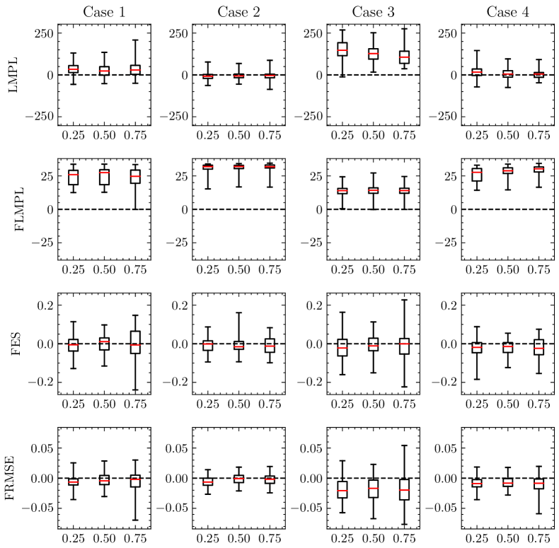
Figure 3: Difference of estimation accuracy between D-FS-CSN and D-CAR for each case (x-axis denotes the values of $\rho_{S}$)

5 Application

In the application section, we undertake the identification of Cobb-Douglas production functions for 48 states in the United States spanning the period 1970-1986, following the data outlined in Baltagi (2021). The model is specified as:

$$y_{tk} =\beta_{intercept}+\beta_{\mathrm{KP}}\log\mathrm{KP}_{tk}+\beta_{\mathrm{KH}}\log\mathrm{KH}_{tk}+\beta_{\mathrm{KW}}\log\mathrm{KW}_{tk}$$

$$\qquad+\beta_{\mathrm{KO}}\log\mathrm{KO}_{tk}+\beta_{\mathrm{L}}\log\mathrm{L}_{tk}+\beta_{\mathrm{Unemp}}\mathrm{Unemp}_{tk}+\theta_{tk}+\epsilon_{tk},$$

Here, $y$ is the logarithm of the gross state product, and the features include the private capital stock ($\mathrm{KP}$), highways and streets ($\mathrm{KH}$), water and sewer facilities ($\mathrm{KW}$), other public buildings and structures ($\mathrm{KO}$), the nonagricultural payroll employment ($\mathrm{L}$), and the state unemployment rate ($\mathrm{Unemp}$). All features except the unemployment rate are expressed in natural logarithms. Figure 4 displays the values of $y$, namely, the logarithm of the gross state product for each state in 1970, 1977, and 1984. The data spanning from 1970 to 1984 is utilized as the training dataset, while the data from 1985 to 1986 is employed to validate the predictive accuracy of the models.

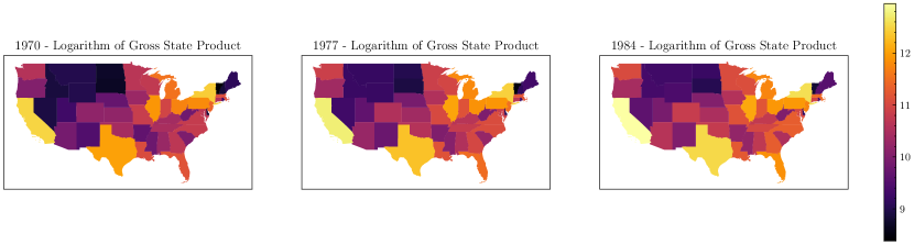
Figure 4: Logarithm of gross state product in 1970, 1977, 1984

In the D-FS-CSN model, $\theta$ follows equation (5), whereas in the D-CAR model, it adheres to equation (1). The prior distribution used for both models is consistent with that utilized in the simulation studies.

Table 2 displays the 5%, 50%, and 95% percentile of samples drawn from the posterior distributions of parameters for both the D-FS-CSN and D-CAR models. Notably, the estimated results for $\lambda$ are around 1.5, suggensting that even after taking the logarithm of the raw data, a significant skewness persists. The quantiles of the posterior distributions for other parameters are generally exhibit similar patterns, although there is a slightly variation observed in the estimates of the regression coefficients.

	D-FS-CSN			D-CAR
Parameter	5%	50%	95%	5%	50%	95%
$\beta_{intercept}$	1.1467	1.3248	1.5009	1.0373	1.1912	1.3602
$\beta_{\mathrm{KP}}$	0.3522	0.3867	0.4185	0.3709	0.4042	0.4363
$\beta_{\mathrm{KH}}$	0.0754	0.1178	0.1601	0.1017	0.1438	0.1867
$\beta_{\mathrm{KW}}$	0.0543	0.0808	0.1084	0.0529	0.0794	0.1048
$\beta_{\mathrm{KO}}$	-0.0489	-0.0179	0.0127	-0.0374	-0.0075	0.0220
$\beta_{\mathrm{L}}$	0.4714	0.5136	0.5591	0.4291	0.4705	0.5098
$\beta_{\mathrm{Unemp}}$	-0.0087	-0.0062	-0.0036	-0.0097	-0.0071	-0.0046
$\sigma^{2}(\times 10^{-2})$	0.0191	0.0228	0.0272	0.0195	0.0234	0.0278
$\tau^{2}(\times 10^{-2})$	0.2129	0.2405	0.2706	0.2211	0.2505	0.2813
$\rho_{S}$	0.6172	0.7390	0.8364	0.6461	0.7551	0.8517
$\rho_{T}$	0.9284	0.9528	0.9773	0.9285	0.9541	0.9781
$\lambda$	1.0709	1.4746	1.9199

Table 2: Estimation results of parameters

Figure 5 displays the 5%, 50%, and 95% percentile points of the posterior distribution of $\theta$ for each state in 1970, 1977, and 1984 under the D-FS-CSN model and the D-CAR model. The figures reveal that while it is evident that although the trends in the estimates of $\theta$ are similar between the two models, the actual values differ significantly. For example, the posterior median of $\theta$ for Wyoming in 1970 under the D-CAR model is approximately $0.15$, whereas it is about $0.25$ under the D-FS-CSN model. Moreover, certain states are dipicted in much brighter colors under the D-FS-CSN model. For instance, Wyoming around 1970 is depicted in a brighter color, indicating higher productivity than expected based on its capital and infrastructure. In 1970, Wyoming was the second least populous state (United States Census Bureau, 1973). It generally exhibited low feature values, with $L$ being the smallest. However, due to its abundant resources such as coal, crude oil, and natural gas (U.S. Energy Information Administration, 2023), Wyoming demonstrated a total production that surpassed predictions based on its features. The states appearing in brighter colors under the D-FS-CSN model suggest that this model assigns greater probability to positive values compared to the D-CAR model, due to $\lambda$ being positive.

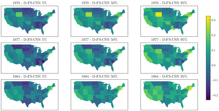
(a) Estimation results of D-FS-CSN model

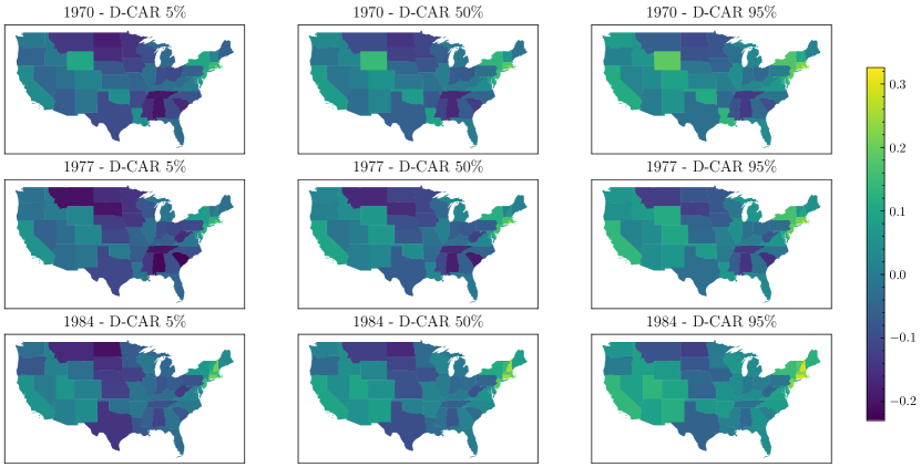
(b) Estimation results of D-CAR model

Figure 5: 5%, 50% and 95% percentile points of $\theta$ for each state in 1970, 1977 and 1984

Finally, Table 3 presents the evaluation of predictive accuracy. Improvements are observed across all metrics. Due to the small observational noise, the improvement margins for FES and FRMSE are modest, but FLPML shows a particularly significant improvement. This suggests that the D-FS-CSN model is superior both in terms of fit to the training data and predictive accuracy.

	LMPL	FLMPL	FES	FRMSE$(\times 10^{-2})$
D-FS-CSN	1910.492	349.609	0.231	5.822
D-CAR	1906.128	292.199	0.233	5.921

Table 3: Prediction accuracy in application

6 Conclusion

In this study, we propose the D-FS-CSN model by combining the D-CAR model and the FS-CSN distribution, enabling the treatment of spatio-temporal structure and skewness while preserving mean and variance, crucial for maintaining parameters interpretable (see Section 1). Moreover, due to its natural representation as an AR model, we proposed an efficient sampling method from the posterior distribution. Additionallly, we adopted the spatial covariance matrix decomposition to use the matrix square root instead of the Cholesky decomposition, accommodating variations in the spatial ordering. We also derived the measures of multivariate skewness and kurtosis for FS-CSN, emphasizing that Mardia’s skewness and kurtosis are independent of the mean and variance, depending solely on $\lambda$.

In simulation studies, we investigated the parameter estimation performance of the proposed D-FS-CSN model for each case and compared it with the performance of the D-CAR model. The results revealed that the advantages of using the D-FS-CSN model are more pronounced when the observational noise $\sigma^{2}$ is small, and the skewness-determining $\lambda$ is large.

For the application to real data, we applied the D-FS-CSN model to estimate Cobb-Douglas production functions for each state in the United States. We compared the estimation results and performance with those of the D-CAR model. Despite employing logarithmic transformations, the results indicated some degree of skewness. Both LMPL and FLPML demonstrated a better fit with the D-FS-CSN model, suggesting its superiority in terms of both fit and prediction. Considering that the D-FS-CSN model includes the D-CAR model as a subclass, it can be a viable option even when logarithmic transformations are used.

Future development could include adapting the proposed model to allow the skewness parameter $\lambda$ by vary by location and time. Additionally, since the D-CAR model is often applied to observations of count data or binary data, its applicability to such cases could also be considered.

The implementation in Julia is available on GitHub (https://github.com/Kuno3/DFsCsn).

Appendix A Proof of proposition 3.1

Consider a random variable $z=(z_{1},\ldots,z_{p})^{\prime}$ following the $\textrm{FS-CSN}_{p}(\mu,\Omega,\lambda,\Omega^{s})$. Let the permuted random variable of $z$ be $\tilde{z}=(z_{\xi(1)},\ldots,z_{\xi(p)})^{\prime}$, where $P$ is a permutation matrix such that $Pz=\tilde{z}$. $z$ can also be expressed as follows:

$$z =\mu-b\delta\gamma\Omega^{s}1_{p}+\psi+\frac{\gamma\lambda}{1+\lambda^{2}}\Omega^{s}\alpha$$

$$\psi \sim N_{p}\left(0_{p},\frac{\gamma^{2}}{1+\lambda^{2}}\Omega\right)$$

$$\alpha \sim TN_{p}\left(0_{p},(1+\lambda^{2})I_{p}\right).$$

Considering that $PP^{\prime}=P^{\prime}P=I_{p}$,

$$Pz =P\mu-b\delta\gamma P\Omega^{s}1_{p}+Pv+\frac{\gamma\lambda}{1+\lambda^{2}}P\Omega^{s}\alpha$$

$$=P\mu-b\delta\gamma P\Omega^{s}P^{\prime}P1_{p}+Pv+\frac{\gamma\lambda}{1+\lambda^{2}}P\Omega^{s}P^{\prime}P\alpha.$$

Let $\tilde{\mu}=P\mu$, $\tilde{\alpha}=Pu$, $\tilde{\psi}=Pv$, and $\tilde{\Omega}=P\Omega P^{\prime}$. Given that $P1_{p}=1_{p}$ and $\tilde{\Omega}^{s}=P\Omega^{s}P^{\prime}$,

$$Pz =\tilde{\mu}-b\delta\gamma\tilde{\Omega}^{s}1_{p}+\tilde{\psi}+\frac{\gamma\lambda}{1+\lambda^{2}}\tilde{\Omega}^{s}\tilde{\alpha}$$

$$\tilde{\psi} \sim N_{p}\left(0_{p},\frac{\gamma^{2}}{1+\lambda^{2}}\tilde{\Omega}\right)$$

$$\tilde{\alpha} \sim TN_{p}\left(0_{p},(1+\lambda^{2})I_{p}\right).$$

From the above decomposition, $Pz$ is identical to the random variable $\tilde{z}$. However, when employing the Cholesky decomposition, $\tilde{\Omega}^{c}$ does not equal $P\Omega^{c}P^{\prime}$, and therefore they are not identical.

Appendix B Proof of proposition 3.2

Let $R_{t,1:T}$ and $R_{t,1:T}^{c}$ be the $t$th row of $R$ and $R$. When $\theta_{1:T}$ follows $\textrm{FS-CSN}_{TK}(0_{TK},R\otimes\Omega,\lambda,R^{c}\otimes\Omega^{s})$, $\theta_{t}$ is

$$\theta_{t} =-b\delta\gamma R_{t,1:T}^{c}\otimes\Omega^{s}1_{TK}+\psi_{t}+\frac{\gamma\lambda}{1+\lambda^{2}}R_{t,1:T}^{c}\otimes\Omega^{s}\alpha_{1:T}$$

$$\psi_{t} \sim N_{K}\left(0_{K},\frac{\gamma^{2}}{1+\lambda^{2}}R_{t,t}\otimes\Omega\right)$$

$$\alpha_{1:T} \sim TN_{TK}\left(0_{TK},(1+\lambda^{2})I_{TK}\right).$$

The elements of $R^{c}$ are

$$R^{c}_{t,t}=1 \text{ for }t=1,\ldots,T,$$

$$R^{c}_{t_{1},t_{2}}=\rho_{T}^{t_{2}-t_{1}} \text{ for }1\leq t_{1}<t_{2}\leq T,$$

$$R^{c}_{t_{2},t_{1}}=0 \text{ for }1\leq t_{1}<t_{2}\leq T.$$

Then,

$$-b\delta\gamma R_{t,1:T}^{c}\otimes\Omega^{s}1_{TK} =\rho_{T}\left(-b\delta\gamma R_{t-1,1:T}^{c}\otimes\Omega^{s}1_{TK}\right)-b\delta\gamma\Omega^{s}1_{K}$$

$$\frac{\gamma\lambda}{1+\lambda^{2}}R_{t,1:T}^{c}\otimes\Omega^{s}\alpha_{1:T} =\rho_{T}\left(\frac{\gamma\lambda}{1+\lambda^{2}}R_{t-1,1:T}^{c}\otimes\Omega^{s}\alpha_{1:T}\right)+\frac{\gamma\lambda}{1+\lambda^{2}}\Omega^{s}u_{t}$$

Furthermore, $\psi_{t}=\rho_{T}\psi_{t-1}+\psi$, where $\psi_{t-1}\sim N_{K}\left(0_{K},\gamma^{2}/(1+\lambda^{2})R_{t-1,t-1}\otimes\Omega\right)$ and $\psi\sim N_{K}\left(0_{K},\gamma^{2}/(1+\lambda^{2})\Omega\right)$. Therefore,

$$\theta_{t} =\rho_{T}(-b\delta\gamma R_{t-1,1:T}^{c}\otimes\Omega^{s}1_{TK}+\psi_{t-1}+\frac{\gamma\lambda}{1+\lambda^{2}}R_{t-1,1:T}^{c}\otimes\Omega^{s}\alpha_{1:T})$$

$$\quad-b\delta\gamma\Omega^{s}1_{K}+\psi+\frac{\gamma\lambda}{1+\lambda^{2}}\Omega^{s}u_{t}.$$

This means

$$\theta_{t} =\rho_{T}\theta_{t-1}+w_{t}$$

$$w_{t} \sim\textrm{FS-CSN}_{K}(0_{K},\Omega,\lambda,\Omega^{s}).$$

Appendix C Proof of proposition 3.3

Let $m_{i}(x)$ be the $i$th moment of a random variabble $x$. That is

$$m_{1}(x) =\mathbb{E}\left[x\right],$$

$$m_{2}(x) =\mathbb{E}\left[xx^{\prime}\right],$$

$$m_{3}(x) =\mathbb{E}\left[x\otimes x^{\prime}\otimes x\right],$$

$$m_{4}(x) =\mathbb{E}\left[x\otimes x^{\prime}\otimes x\otimes x^{\prime}\right].$$

When $z$ follows $\textrm{FS-CSN}_{p}(\mu,\Omega,\lambda,\Omega^{1/2})$, $z$ can be expressed as

$$z =\mu+\psi+\Lambda\left(\alpha-\frac{b\lambda}{\delta}1_{p}\right),$$

$$\psi \sim N_{p}\left(0_{p},\Psi\right)$$

$$\alpha \sim TN_{p}\left(0_{p},(1+\lambda^{2})I_{p}\right)$$

where $\Lambda=(\gamma\delta^{2}/\lambda)\Omega^{1/2}$ and $\Psi=(\gamma^{2}\delta^{2}/\lambda^{2})\Omega$. Let $\alpha_{0}$ be $\alpha-(b\lambda/\delta)1_{p}$, according to Arellano-Valle and Azzalini (2022), then

$$\mathrm{MS}(z) =\mathrm{tr}\left((M_{00}\otimes M_{00})m_{3}(\alpha_{0})M_{00}m_{3}(\alpha_{0})^{\prime}\right),$$

where $M_{00}=\Lambda^{\prime}\Omega^{-1}\Lambda=\gamma^{2}\delta^{4}/\lambda^{2}I_{p}$. Since $\alpha_{0}$ follows a truncated normal distribution independently across dimensions, the elements of $m_{3}(\alpha_{0})$ are as follows:

$$m_{3}(\alpha_{0})_{i,p(i-1)+i}=b^{2}(2b^{2}-1)^{2}\frac{\lambda^{3}}{\delta^{3}} \text{ for }i=1,\ldots,p,$$

$$m_{3}(\alpha_{0})_{i,j}=0 \text{ others }.$$

Therefore,

$$\mathrm{MS}(z) =pb^{2}(2b^{2}-1)^{2}\delta^{6}\gamma^{6}.$$

Similarly,

$$\mathrm{MK}(z) =\mathrm{tr}\left(m_{4}(\alpha_{0})(M_{00}\otimes M_{00})\right)+4\mathrm{tr}\left(m_{2}(\alpha_{0})M_{01}M_{01}^{\prime}\right)$$

$$\quad+2\mathrm{tr}\left(m_{2}(\alpha_{0})M_{00}\right)\mathrm{tr}(M_{11})+\mathrm{tr}(M_{11})^{2}+2\mathrm{tr}(M_{11}^{2}),$$

where $M_{01}M_{01}^{\prime}=\Lambda^{\prime}\Omega^{-1}\Psi\Omega^{-1}\Lambda=\gamma^{4}\delta^{6}/\lambda^{4}I_{p}$, $\mathrm{tr}(M_{11})=\mathrm{tr}(\Psi\Omega^{-1})=p\gamma^{2}\delta^{2}/\lambda^{2}$, $\mathrm{tr}(M_{11}^{2})=\mathrm{tr}(\Psi\Omega^{-1}\Psi\Omega^{-1})=p\gamma^{4}\delta^{4}/\lambda^{4}$,

$$m_{4}(\alpha_{0})_{p(i-1)+i,p(i-1)+i}=\frac{\lambda^{4}}{\delta^{4}}\left(3-2b^{2}-3b^{4}\right) \text{ for }i=1,\ldots,p,$$

$$m_{4}(\alpha_{0})_{p(i-1)+j,p(i-1)+j}=\frac{(1-b^{2})^{2}\lambda^{4}}{\delta^{4}} \text{ for }i,j=1,\ldots,p,\text{ and }i\neq j,$$

$$m_{4}(\alpha_{0})_{i,j}=0 \text{ others },$$

and $m_{2}(\alpha_{0})=(1-b^{2})\lambda^{2}/\delta^{2}I_{p}$. Therefore,

$$\mathrm{MK}(z) =p\frac{\gamma^{4}\delta^{8}}{\lambda^{4}}\frac{\lambda^{4}}{\delta^{4}}\left(3-2b^{2}-3b^{4}\right)+p(p-1)\frac{\gamma^{4}\delta^{8}}{\lambda^{4}}\frac{(1-b^{2})^{2}\lambda^{4}}{\delta^{4}}$$

$$\quad+4p\frac{\gamma^{4}\delta^{6}}{\lambda^{4}}\frac{(1-b^{2})\lambda^{2}}{\delta^{2}}+2p^{2}\frac{(1-b^{2})\lambda^{2}}{\delta^{2}}\frac{\gamma^{2}\delta^{4}}{\lambda^{2}}\frac{\gamma^{2}\delta^{2}}{\lambda^{2}}+p^{2}\frac{\gamma^{4}\delta^{4}}{\lambda^{4}}+2p\frac{\gamma^{4}\delta^{4}}{\lambda^{4}},$$

$$=p\left(p+2+2b^{2}(2-3b^{2})\delta^{4}\gamma^{4}\right).$$

From here, when $\lambda=0$, $\mathrm{MS}(z)=0$ and $\mathrm{MK}(z)=p(p+2)$. Additionaly, the following properties naturally emerge.

$$\lim_{\lambda\rightarrow\infty}\mathrm{MS}(z) =p\left(\frac{b(2b^{2}-1)}{(1-b^{2})^{3/2}}\right)^{2},$$

$$\lim_{\lambda\rightarrow\infty}\mathrm{MK}(z) =p\left(p+2+\frac{2b^{2}(2-3b^{2})}{(1-b^{2})^{2}}\right).$$

Appendix D Full process of MCMC

To achieve efficient sampling, this paper utilizes block Gibbs sampling. The sampling method of $\theta_{1:T}|y_{1:T},\beta,\sigma,\Omega,\rho_{T},\lambda$ and $\alpha_{t}|\theta_{1:T},\Omega,\rho_{T},\lambda$ is described in section 3. Moreover, $p(\beta|y_{1:T},\theta_{1:T},\sigma^{2})$, $p(\sigma^{2}|y_{1:T},\theta_{1:T},\beta)$, $p(\rho_{T}|\theta_{1:T},\tau^{2},\rho_{S})$ can be calculated analytically. $\beta|y_{1:T},\theta_{1:T},\sigma^{2}$ is distributed with $N(\mu_{\beta},\Sigma_{\beta})$, where

$$\Sigma_{\beta} =\left(\frac{1}{\sigma^{2}}X_{1:T}^{T}X_{1:T}+\frac{1}{\sigma_{\beta}^{2}}I_{r}\right)^{-1},$$

$$\mu_{\beta} =\frac{1}{\sigma^{2}}\Sigma_{\beta}X_{1:T}^{T}(y_{1:T}-\theta_{1:T}).$$

$\sigma^{2}|y_{1:T},\theta_{1:T},\beta$ is distributed with $\mathrm{InverseGamma}(a_{\sigma^{2}}+KT/2,b_{\sigma^{2}}+(y_{1:T}-\theta_{1:T}-X_{1:T}\beta)^{\prime}(y_{1:T}-\theta_{1:T}-X_{1:T}\beta)/2)$. $\rho_{T}|\theta_{1:T},\alpha_{1:T},\tau^{2},\Omega$ follows a normal distribution truncated between $0$ and $1$, with mean $\mu_{\rho_{T}}$ and variance $\sigma_{\rho_{T}}^{2}$, where

$$\sigma_{\rho_{T}}^{2} =\left(\frac{1+\lambda^{2}}{\gamma^{2}}\sum_{t=2}^{T}\theta_{t-1}^{\prime}\Sigma^{-1}\theta_{t-1}\right)^{-1},$$

$$\mu_{\rho_{T}} =\frac{1+\lambda^{2}}{\gamma^{2}}\sigma_{\rho_{T}}^{2}\sum_{t=2}^{T}\theta_{t-1}^{\prime}\Sigma^{-1}\left(\theta_{t}+b\delta\gamma\Omega^{s}1_{K}-\frac{c\lambda}{1+\lambda^{2}}\Sigma^{1/2}\alpha_{t}\right).$$

The parameters of $\Omega$ are sampled by Metropolis-Hasting or Hamiltonian Monte Carlo.

References

• Allard and Naveau (2007) Allard, D., Naveau, P., 2007. A new spatial skew-normal random field model. Commun. Stat.—Theory and Methods 36, 1821–1834.
• Anselin (2022) Anselin, L., 2022. Spatial econometrics, in: Rey, S.J., Franklin, R.S. (Eds.), Handbook of Spatial Analysis in the Social Sciences. Edward Elgar Publishing, Cheltenham, pp. 101–122.
• Arellano-Valle and Azzalini (2006) Arellano-Valle, R.B., Azzalini, A., 2006. On the unification of families of skew-normal distributions. Scand. J. Stat. 33, 561–574.
• Arellano-Valle and Azzalini (2022) Arellano-Valle, R.B., Azzalini, A., 2022. Some properties of the unified skew-normal distribution. Stat. Pap. 63, 461–487.
• Azzalini (1985) Azzalini, A., 1985. A class of distributions which includes the normal ones. Scand. J. Stat. 12, 171–178.
• Azzalini and Capitanio (1999) Azzalini, A., Capitanio, A., 1999. Statistical applications of the multivariate skew normal distribution. J. R. Stat. Soc. Ser. B Stat. Methodol. 61, 579–602.
• Baltagi (2021) Baltagi, B.H., 2021. Econometric Analysis of Panel Data. 6th ed., Springer, Berlin.
• Best et al. (2005) Best, N., Richardson, S., Thomson, A., 2005. A comparison of bayesian spatial models for disease mapping. Stat. Methods Med. Res. 14, 35–59.
• Botev (2017) Botev, Z.I., 2017. The normal law under linear restrictions: Simulation and estimation via minimax tilting. J. R. Stat. Soc. Ser. B Stat. Methodol. 79, 125–148.
• Carter and Kohn (1994) Carter, C.K., Kohn, R., 1994. On gibbs sampling for state space models. Biometrika 81, 541–553.
• Dormann et al. (2007) Dormann, C.F., McPherson, J.M., Araújo, M.B., Bivand, R., Bolliger, J., Carl, G., Davies, R.G., Hirzel, A., Jetz, W., Daniel Kissling, W., et al., 2007. Methods to account for spatial autocorrelation in the analysis of species distributional data: a review. Ecography 30, 609–628.
• Frühwirth-Schnatter (1994) Frühwirth-Schnatter, S., 1994. Data augmentation and dynamic linear models. J. Time Ser. Anal. 15, 183–202.
• Gelfand et al. (2010) Gelfand, A.E., Diggle, P., Guttorp, P., Fuentes, M., 2010. Handbook of Spatial Statistics. CRC press.
• Genton and Zhang (2012) Genton, M.G., Zhang, H., 2012. Identifiability problems in some non-gaussian spatial random fields. Chil. J. Stat. 3, 171–179.
• Gneiting and Raftery (2007) Gneiting, T., Raftery, A.E., 2007. Strictly proper scoring rules, prediction, and estimation. J. Amer. Statist. Assoc. 102, 359–378.
• Khaledi et al. (2023) Khaledi, M.J., Zareifard, H., Boojari, H., 2023. A spatial skew-gaussian process with a specified covariance function. Stat. Probab. Lett. 192, 109681.
• Kim and Mallick (2004) Kim, H.M., Mallick, B.K., 2004. A bayesian prediction using the skew gaussian distribution. J. Stat. Plan. Inference 120, 85–101.
• Lee et al. (2018) Lee, D., Rushworth, A., Napier, G., 2018. Spatio-temporal areal unit modeling in r with conditional autoregressive priors using the carbayesst package. J. Stat. Softw. 84, 1–39.
• Márquez-Urbina and González-Farías (2022) Márquez-Urbina, J.U., González-Farías, G., 2022. A flexible special case of the csn for spatial modeling and prediction. Spatial Stat. 47, 100556.
• Schmidt et al. (2017) Schmidt, A.M., Gonçalves, K.C.M., Velozo, P.L., 2017. Spatiotemporal models for skewed processes. Environmetrics 28, e2411.
• Tagle et al. (2019) Tagle, F., Castruccio, S., Crippa, P., Genton, M.G., 2019. A non-gaussian spatio-temporal model for daily wind speeds based on a multi-variate skew-t distribution. J. Time Ser. Anal. 40, 312–326.
• United States Census Bureau (1973) United States Census Bureau, 1973. 1970 census of population: Characteristics of the population. https://www.census.gov/library/publications/1973/dec/population-volume-1.html. (accessed 25 May 2024).
• U.S. Energy Information Administration (2023) U.S. Energy Information Administration, 2023. Production - state energy data system (seds). https://www.eia.gov/state/seds/seds-data-complete.php. (accessed 25 May 2024).
• Wang et al. (2023) Wang, K., Arellano-Valle, R.B., Azzalini, A., Genton, M.G., 2023. On the non-identifiability of unified skew-normal distributions. Stat 12, e597.
• Yan et al. (2020) Yan, Y., Jeong, J., Genton, M.G., 2020. Multivariate transformed gaussian processes. Jpn. J. Stat. Data Sci. 3, 129–152.