Set Estimation from Projected Multidimensional Random Variables with Application to a Discrete-Time Skorokhod Problem

Abstract.

This paper deals with sufficient conditions on the distribution of the random variable $H$, in the model $X=\Pi_{C}(H)$, for the convex hull $\widehat{C}_{N}$ of $N$ independent copies of $X$ to be a consistent estimator of the convex body $C$ with a rate of convergence. The convergence of $\widehat{C}_{N}$ is established for the Hausdorff distance under a uniform condition on the distribution of $H$, but also in a pointwise sense under a less demanding condition. Some of these convergence results on $\widehat{C}_{N}$ are applied to the estimation of the time-dependent constraint set involved in a discrete-time Skorokhod problem.

^†Université Paris Nanterre, CNRS, Modal’X, 92001 Nanterre, France.

1. Introduction

Consider $m\in\mathbb{N}^{*}$, a convex body $C$ of $\mathbb{R}^{m}$, a $\mathbb{R}^{m}$-valued random variable $H$, and

(1) $$X=\Pi_{C}(H).$$

The random variable $X$ may be interpreted as $H$ censored by $C$. For instance, $X$ could model the location recorded by a sensor of range $\rho>0$, of a target which exact location in $\mathbb{R}^{3}$ is modeled by $H$, by taking $C=\overline{B}_{d}(0,\rho)$. A natural estimator of $C$ is given by

$$\widehat{C}_{N}:={\rm conv}\{X_{1},\dots,X_{N}\},$$

where $X_{1},\dots,X_{N}$ are $N\in\mathbb{N}^{*}$ independent copies of the random variable $X$. First, our paper deals with sufficient conditions on the distribution of $H$ for $\widehat{C}_{N}$ to be consistent with a rate of convergence. In the literature on set estimation, the convergence of sequences of random convex bodies is established for the Hausdorff (or the Nikodym) distance (see Dümbgen and Walther [9], Casal [4], Cuevas [7], Brunel [3], or Brunel [2] for a nice survey). Following this line, our paper deals with the consistency of $\widehat{C}_{N}$, with a rate of convergence, for the Hausdorff distance (see Sections 2 and 3). Consider two convex bodies $K$ and $L$ of $\mathbb{R}^{m}$ such that $L\subset K$. If

$$d(\mathbf{x},L)=0\textrm{ $;$ }\forall\mathbf{x}\in{\rm int}(K),$$

then ${\rm int}(K)\subset L$, leading to $K=L$ because $K$ and $L$ are closed subsets of $\mathbb{R}^{m}$. For this reason, it makes sense to say that a sequence $(L_{n})_{n\in\mathbb{N}}$ of random convex-compact subsets of $K$ converges pointwise (in probability) to $K$ if and only if,

$$d(\mathbf{x},L_{n})\xrightarrow[n\rightarrow\infty]{\mathbb{P}}0\textrm{ $;$ }\forall\mathbf{x}\in{\rm int}(K).$$

So, Section 3 also deals with a sufficient condition on the distribution of $H$ for $\widehat{C}_{N}$ to be a pointwise converging estimator of $C$ with an explicit rate. As for the estimation of a probability measure’s support (see Brunel [3], Assumption 1 and Proposition 1), the condition on $\mathbb{P}_{H}(\overline{B}_{d}(\mathbf{x},\cdot)\cap{\rm int}(C))$, sufficient to establish the convergence of $\widehat{C}_{N}$ for the Hausdorff distance, is uniform in $\mathbf{x}\in C$, and then harder to check in applications than that sufficient to establish its pointwise convergence. For $C=C_{1}\times\dots\times C_{m}$, where $C_{1},\dots,C_{m}$ are convex bodies of $\mathbb{R}$, Section 3 finally deals with convergence results (for the Hausdorff distance) on the alternative estimator $\widetilde{C}_{N}=\widehat{C}_{1,N}\times\dots\times\widehat{C}_{m,N}$, inherited from those established on $\widehat{C}_{N}$ when $m=1$ (see Section 2). Now, consider the discrete-time Skorokhod problem

(2) $$\left\{\begin{array}[]{rcl}\overline{\tt X}_{j+1}&=&\Pi_{\texttt{C}(t_{j+1})}(\overline{\tt X}_{j}+b(\overline{\tt X}_{j})\Delta_{n}+\sigma(\overline{\tt X}_{j})(\texttt{W}_{t_{j+1}}-\texttt{W}_{t_{j}}))\\ \overline{\tt X}_{0}&\equiv&\mathbf{x}_{0}\in\texttt{C}(0)\end{array}\right.\textrm{$;$ }j\in J_{n}\backslash\{n\},$$

where $b$ (resp. $\sigma$) is a Lipschitz continuous map from $\mathbb{R}^{m}$ into itself (resp. ${\rm GL}_{m}(\mathbb{R})$), W is a $m$-dimensional Brownian motion, $\texttt{C}:\mathbb{R}_{+}\rightrightarrows\mathbb{R}^{m}$ is a convex-body-valued multifunction, $J_{n}:=\{0,\dots,n\}$ with $n\in\mathbb{N}^{*}$, $\Delta_{n}:=T/n$ with $T>0$, and $t_{j}:=j\Delta_{n}$ for every $j\in J_{n}$. Thanks to the properties of $\widehat{C}_{N}$ established in Sections 2 and 3, Section 4 deals with pointwise convergence results on the estimator

$$\widehat{\tt C}_{N,j}:={\rm conv}\{\overline{\tt X}_{j}^{1},\dots,\overline{\tt X}_{j}^{N}\}\textrm{ $;$ }j\in J_{n}\backslash\{0\}$$

of $\texttt{C}(t_{j})$, where $\overline{\tt X}^{1},\dots,\overline{\tt X}^{N}$ are $N$ independent copies of $\overline{\tt X}$. Under appropriate regularity conditions on C (see Bernicot and Venel [1], Theorems 3.9 and 4.6), when $n\rightarrow\infty$, the solution of Problem (2) converges uniformly to the solution of the following continuous-time Skorokhod reflection problem:

$$\texttt{X}_{t} = \int_{0}^{t}b(\texttt{X}_{s})ds+\int_{0}^{t}\sigma(\texttt{X}_{s})d\texttt{W}_{s}+\texttt{Y}_{t}$$

$$\hskip 56.9055pt{\rm with}\quad\left\{\begin{array}[]{rcl}-\dot{\tt Y}_{t}&\in&\mathcal{N}_{\texttt{C}(t)}(\texttt{X}_{t})\quad|\textrm{D}\texttt{Y}|\textrm{-a.e.}\\ \texttt{Y}_{0}(\cdot)&\equiv&\mathbf{x}_{0}\end{array}\right.\textrm{$;$ }t\in[0,T]$$

where, for every convex body $K$ of $\mathbb{R}^{m}$, $\mathcal{N}_{K}(\mathbf{x})$ is the normal cone of $K$ at point $\mathbf{x}\in\mathbb{R}^{m}$, and for every continuous function of bounded variation $\varphi:[0,T]\rightarrow\mathbb{R}^{m}$,

$$\dot{\varphi}:=\frac{d\textrm{D}\varphi}{d|\textrm{D}\varphi|}$$

with $\textrm{D}\varphi$ the differential measure of $\varphi$ and $|\textrm{D}\varphi|$ its variation measure. For this reason, our paper is also part of the intensively investigated research field of the copies-based statistical inference for diffusion processes (see Comte and Genon-Catalot [6], Marie and Rosier [11], Denis et al. [8], etc.). For another example of estimator in a reflected diffusion model computed from observations of the corresponding approximation scheme, the reader may refer to Cattiaux et al. [5].

Some proofs, especially the longest ones, are postponed to Appendix A.

Notations:

• The space of the $m\times m$ invertible matrices with real entries is denoted by ${\rm GL}_{m}(\mathbb{R})$.

• The orthogonal projection from $\mathbb{R}^{m}$ onto a convex body $K$ of $\mathbb{R}^{m}$ is denoted by $\Pi_{K}(\cdot)$.

• The Hausdorff distance on $\mathcal{P}(\mathbb{R}^{m})$, associated to the Euclidean distance $d$ on $\mathbb{R}^{m}$, is denoted by $d_{\rm H}$:

  $$d_{\rm H}(A,B)=\max\left\{\sup_{\mathbf{x}\in A}d(\mathbf{x},B)\textrm{ $;$ }\sup_{\mathbf{x}\in B}d(\mathbf{x},A)\right\}\textrm{ $;$ }\forall A,B\in\mathcal{P}(\mathbb{R}^{m}).$$

• The Tchebychev distance on $\mathbb{R}^{m}$ is denoted by $d_{\infty}$:

  $$d_{\infty}(\mathbf{x},\mathbf{y})=\max_{j=1}^{m}|\mathbf{y}_{j}-\mathbf{x}_{j}|\textrm{ $;$ }\forall\mathbf{x},\mathbf{y}\in\mathbb{R}^{m}.$$

• The Lebesgue measure on $\mathbb{R}^{m}$ is denoted by $\lambda_{m}$, and $\lambda:=\lambda_{1}$.

2. The case $m=1$

Throughout this section, let us assume that $m=1$. Then, $C=[I,S]$ with $I,S\in\mathbb{R}$ satisfying $I<S$, and

$$\widehat{C}_{N} = [\widehat{I}_{N},\widehat{S}_{N}]\quad{\rm with}\quad\widehat{I}_{N}=\min\{X_{1},\dots,X_{N}\}$$

$$\hskip 142.26378pt{\rm and}\quad\widehat{S}_{N}=\max\{X_{1},\dots,X_{N}\}.$$

So, here, $X$ is a censored random variable in the usual sense. In order to prove convergence results on $\widehat{C}_{N}$ in Proposition 2.2 and Corollary 2.3, let us first establish a suitable relationship between the distribution function of $H$ and that of $X$.

Lemma 2.1.

Let $F$ (resp. $\Phi$) be the distribution function of $X$ (resp. $H$). For every $x\in\mathbb{R}$,

$$F(x)=\Phi(x)\mathbb{1}_{I\leqslant x<S}+\mathbb{1}_{x\geqslant S}.$$

Proof.

First, for any $x\in\mathbb{R}$, since $\{I<H<S\}\subset\{X=H\}$,

$$F(x) = \mathbb{P}(X\leqslant x,H\in(I,S))+\mathbb{P}(X\leqslant x,H\not\in(I,S))$$

$$= \mathbb{P}(H\leqslant x,I<H<S)+\mathbb{P}(X\leqslant x,H\leqslant I)+\mathbb{P}(X\leqslant x,H\geqslant S).$$

Moreover,

$$\mathbb{P}(H\leqslant x,I<H<S)=\mathbb{P}(I<H\leqslant x)\mathbb{1}_{I<x<S}+\mathbb{P}(I<H<S)\mathbb{1}_{x\geqslant S}$$

and, since $\{H\leqslant I\}=\{X=I\}$ and $\{H\geqslant S\}=\{X=S\}$,

$$\mathbb{P}(X\leqslant x,H\leqslant I)+\mathbb{P}(X\leqslant x,H\geqslant S)=\mathbb{P}(H\leqslant I)\mathbb{1}_{x\geqslant I}+\mathbb{P}(H\geqslant S)\mathbb{1}_{x\geqslant S}.$$

Thus,

$$F(x) = \mathbb{P}(I<H\leqslant x)\mathbb{1}_{I<x<S}+\mathbb{P}(H\leqslant I)\mathbb{1}_{x\geqslant I}$$

$$\hskip 71.13188pt+(\mathbb{P}(I<H<S)+\mathbb{P}(H\geqslant S))\mathbb{1}_{x\geqslant S}$$

$$= (\mathbb{P}(H\leqslant x)-\mathbb{P}(H\leqslant I))\mathbb{1}_{I<x<S}$$

$$\hskip 71.13188pt+\mathbb{P}(H\leqslant I)(\mathbb{1}_{x=I}+\mathbb{1}_{x>I})+\mathbb{P}(H>I)\mathbb{1}_{x\geqslant S}$$

$$= \mathbb{P}(H\leqslant x)\mathbb{1}_{I\leqslant x<S}+\underbrace{(\mathbb{P}(H\leqslant I)+\mathbb{P}(H>I))}_{=1}\mathbb{1}_{x\geqslant S}.$$

In conclusion,

$$F(x)=\Phi(x)\mathbb{1}_{I\leqslant x<S}+\mathbb{1}_{x\geqslant S}.$$

∎

Now, the following proposition provides a sufficient condition on the distribution function of $H$ for $\widehat{C}_{N}$ to be consistent.

Proposition 2.2.

Assume that

(4) $$\Phi((I,S))\subset(0,1).$$

Then,

$$d_{\rm H}(\widehat{C}_{N},C)\xrightarrow[N\rightarrow\infty]{\mathbb{P}}0.$$

The reader may refer to Section A.1 for a proof of Proposition 2.2. Finally, Proposition 2.3 (resp. Corollary 2.4) provides a sufficient condition on the distribution function of $H$ for $\widehat{S}_{N}$ (resp. $\widehat{C}_{N}$) to converge to $S$ (resp. $C$) with rate $N$.

Proposition 2.3.

Assume that $\Phi$ is continuous and left-differentiable at point $S$, and consider $\delta:=\Phi^{\prime}(S^{-})$.

1. If $\Phi(S)<1$, then

   $$N(\widehat{S}_{N}-S)\xrightarrow[N\rightarrow\infty]{\mathbb{P}}0.$$

2. If $\Phi(S)=1$ and $\delta\neq 0$, then

   $$N\delta(\widehat{S}_{N}-S)\xrightarrow[N\rightarrow\infty]{\mathcal{D}}{\rm Weibull}(1).$$

The reader may refer to Section A.2 for a proof of Proposition 2.3.

Corollary 2.4.

Assume that $\Phi$ is continuous and right-differentiable (resp. left-differentiable) at point $I$ (resp. $S$), and that $\Phi(I)>0$ and $\Phi(S)<1$. Then,

$$Nd_{\rm H}(\widehat{C}_{N},C)\xrightarrow[N\rightarrow\infty]{\mathbb{P}}0.$$

Proof.

First, by Proposition 2.3,

$$N(\widehat{S}_{N}-S)\xrightarrow[N\rightarrow\infty]{\mathbb{P}}0.$$

The same way, since $\Phi$ is continuous and right-differentiable at point $I$, and since $\Phi(I)>0$,

$$N(\widehat{I}_{N}-I)\xrightarrow[N\rightarrow\infty]{\mathbb{P}}0.$$

Thus,

$$Nd_{\rm H}(\widehat{C}_{N},C)=\max\{N|\widehat{S}_{N}-S|,N|\widehat{I}_{N}-I|\}\xrightarrow[N\rightarrow\infty]{\mathbb{P}}0.$$

∎

Remark. If $\Phi(\mathbb{R})\subset(0,1)$, then $H$ fulfills the condition (4) in Proposition 2.2. Moreover, if

(5) $$\Phi\in C^{1}(\mathbb{R})\quad{\rm and}\quad\Phi(\mathbb{R})\subset(0,1),$$

then $H$ fulfills the conditions of Corollary 2.4. For instance, if $H$ is a Gaussian random variable, then it fulfills the sufficient condition (5).

3. The case $m>1$

This section deals with convergence results on an estimator $\widetilde{C}_{N}$ of $C$, simpler than $\widehat{C}_{N}$, when $C$ is a hyper-rectangle (see Section 3.1), and on $\widehat{C}_{N}$ when $C$ is an arbitrary convex body of $\mathbb{R}^{m}$ (see Section 3.2). The results on $\widetilde{C}_{N}$, but not those on $\widehat{C}_{N}$, are consequences of Propositions 2.2 and Corollary 2.4.

3.1. From $m=1$ to hyper-rectangles

Throughout this section,

$$C=\prod_{j=1}^{m}C_{j}$$

where, for every $j\in\{1,\dots,m\}$, $C_{j}:=[I_{j},S_{j}]$ with $I_{j},S_{j}\in\mathbb{R}$ satisfying $I_{j}<S_{j}$.

Notation. In the sequel, for every $j\in\{1,\dots,m\}$, the distribution function of $X_{j}$ (resp. $H_{j}$) is denoted by $F_{j}$ (resp. $\Phi_{j}$).

The following proposition deals with extensions of Proposition 2.2 and Corollary 2.4 to a natural estimator of $C$, simpler than $\widehat{C}_{N}={\rm conv}\{X_{1},\dots,X_{N}\}$.

Proposition 3.1.

Consider

$$\widetilde{C}_{N}:=\prod_{j=1}^{m}\widehat{C}_{N,j}$$

where, for every $j\in\{1,\dots,m\}$,

$$\widehat{C}_{N,j} := [\widehat{I}_{N,j},\widehat{S}_{N,j}]\quad\textrm{with}\quad\widehat{I}_{N,j}=\min\{[X_{1}]_{j},\dots,[X_{N}]_{j}\}$$

$$\hskip 128.0374pt\textrm{and}\quad\widehat{S}_{N,j}=\max\{[X_{1}]_{j},\dots,[X_{N}]_{j}\}.$$

1. If, for every $j\in\{1,\dots,m\}$,

   (6) $$\Phi_{j}((I,S))\subset(0,1),$$

   then

   $$d_{\rm H}(\widetilde{C}_{N},C)\xrightarrow[N\rightarrow\infty]{\mathbb{P}}0.$$

2. Assume that, for every $j\in\{1,\dots,m\}$, $\Phi_{j}$ is continuous and right-differen-tiable (resp. left-differentiable) at point $I_{j}$ (resp. $S_{j}$), and that

   (7) $$\Phi_{j}(I_{j})>0\quad\textrm{and}\quad\Phi_{j}(S_{j})<1.$$

   Then,

   $$Nd_{\rm H}(\widetilde{C}_{N},C)\xrightarrow[N\rightarrow\infty]{\mathbb{P}}0.$$

Proof.

Since $d(\cdot)\leqslant\sqrt{m}d_{\infty}(\cdot)$,

$$\frac{1}{\sqrt{m}}d_{\rm H}(\widetilde{C}_{N},C) = \frac{1}{\sqrt{m}}\sup_{\mathbf{x}\in C}d(\mathbf{x},\widetilde{C}_{N})$$

$$\hskip 56.9055pt{\rm because}\quad\widetilde{C}_{N}\subset C$$

$$= \frac{1}{\sqrt{m}}\sup_{\mathbf{x}\in C}\inf_{\mathbf{y}\in\widetilde{C}_{N}}d(\mathbf{x},\mathbf{y})$$

$$\leqslant \sup_{\mathbf{x}\in C}\left\{\inf_{\mathbf{y}\in\widetilde{C}_{N}}\max_{j=1}^{m}|\mathbf{y}_{j}-\mathbf{x}_{j}|\right\}$$

$$= \sup_{\mathbf{x}\in C}\left\{\max_{j=1}^{m}\inf_{y\in\widehat{C}_{N,j}}|y-\mathbf{x}_{j}|\right\}$$

$$= \max_{j=1}^{m}\left\{\sup_{x\in C_{j}}\inf_{y\in\widehat{C}_{N,j}}|y-x|\right\}=\max_{j=1}^{m}d_{\rm H}(\widehat{C}_{N,j},C_{j}).$$

Thus,

$$d_{\rm H}(\widetilde{C}_{N},C)\xrightarrow[N\rightarrow\infty]{\mathbb{P}}0\quad(\textrm{resp. }Nd_{\rm H}(\widetilde{C}_{N},C)\xrightarrow[N\rightarrow\infty]{\mathbb{P}}0)$$

by applying Proposition 2.2 (resp. Corollary 2.4) to $\widehat{C}_{N,1},\dots,\widehat{C}_{N,m}$ under the condition (6) (resp. (7)). ∎

3.2. Convergence results for an arbitrary convex body

In order to prove pointwise convergence results (resp. convergence results for the Hausdorff distance) on $\widehat{C}_{N}$ in Section 3.2.1 (resp. Section 3.2.2), let us first establish a suitable control of the survival function of

$$d(\mathbf{x},\widehat{C}_{N})\textrm{ $;$ }\mathbf{x}\in C.$$

Lemma 3.2.

For every $\mathbf{x}\in C$ and $\varepsilon>0$,

$$\mathbb{P}(d(\mathbf{x},\widehat{C}_{N})>\varepsilon)\leqslant(1-\mathbb{P}_{H}(\overline{B}_{d}(\mathbf{x},\varepsilon)\cap{\rm int}(C)))^{N}.$$

Proof.

Consider $\mathbf{x}\in C$ and

$$\delta_{N}(\mathbf{x}):=\min_{i=1}^{N}d(\mathbf{x},X_{i}).$$

Since $\{X_{1},\dots,X_{N}\}\subset\widehat{C}_{N}$ by the definition of $\widehat{C}_{N}$,

$$d(\mathbf{x},\widehat{C}_{N}) = \inf_{\mathbf{y}\in\widehat{C}_{N}}d(\mathbf{x},\mathbf{y})$$

$$\leqslant \min_{\mathbf{y}\in\{X_{1},\dots,X_{N}\}}d(\mathbf{x},\mathbf{y})=\delta_{N}(\mathbf{x}).$$

Moreover, for any $\varepsilon>0$,

$$\mathbb{P}(\delta_{N}(\mathbf{x})>\varepsilon) = \mathbb{P}\left(\bigcap_{i=1}^{N}\{d(\mathbf{x},X_{i})>\varepsilon\}\right)$$

$$= \mathbb{P}(d(\mathbf{x},X)>\varepsilon)^{N}=(1-F_{\bf x}(\varepsilon))^{N},$$

where $F_{\bf x}$ is the distribution function of $d(\mathbf{x},X)$, and

$$F_{\bf x}(\varepsilon) = \mathbb{P}(d(\mathbf{x},X)\leqslant\varepsilon,H\in{\rm int}(C))+\mathbb{P}(d(\mathbf{x},X)\leqslant\varepsilon,H\not\in{\rm int}(C))$$

$$\geqslant \mathbb{P}(d(\mathbf{x},H)\leqslant\varepsilon,H\in{\rm int}(C))$$

$$\hskip 85.35826pt{\rm because}\quad\{H\in{\rm int}(C)\}\subset\{X=H\}.$$

Therefore,

$$\mathbb{P}(d(\mathbf{x},\widehat{C}_{N})>\varepsilon)\leqslant(1-\mathbb{P}_{H}(\overline{B}_{d}(\mathbf{x},\varepsilon)\cap{\rm int}(C)))^{N}.$$

∎

3.2.1. Pointwise convergence results

Let us recall that a sequence $(C_{n})_{n\in\mathbb{N}}$ of random convex-compact subsets of $C$ converges pointwise (in probability) to $C$ if and only if,

$$d(\mathbf{x},C_{n})\xrightarrow[n\rightarrow\infty]{\mathbb{P}}0\textrm{ $;$ }\forall\mathbf{x}\in{\rm int}(C).$$

This section deals with pointwise convergence results on $\widehat{C}_{N}$. First, the following proposition provides a sufficient condition on the distribution of $H$ for $\widehat{C}_{N}$ to be pointwise consistent.

Proposition 3.3.

Assume that, for every $\mathbf{x}\in{\rm int}(C)$ and $\varepsilon>0$,

(8) $$\mathbb{P}_{H}(\overline{B}_{d}(\mathbf{x},\varepsilon)\cap{\rm int}(C))>0.$$

Then,

$$d(\mathbf{x},\widehat{C}_{N})\xrightarrow[N\rightarrow\infty]{\mathbb{P}}0\textrm{ $;$ }\forall\mathbf{x}\in{\rm int}(C).$$

Proof.

For any $\mathbf{x}\in{\rm int}(C)$ and $\varepsilon>0$, by Lemma 3.2,

$$\mathbb{P}(d(\mathbf{x},\widehat{C}_{N})>\varepsilon)\leqslant(1-\mathbb{P}_{H}(\overline{B}_{d}(\mathbf{x},\varepsilon)\cap{\rm int}(C)))^{N}.$$

Thus, by Inequality (8),

$$d(\mathbf{x},\widehat{C}_{N})\xrightarrow[N\rightarrow\infty]{\mathbb{P}}0.$$

∎

Let us show (see Section 3.4) that, when $m=1$, the conditions (8) in Proposition 3.3 and (4) in Proposition 2.2 are almost equivalent.

Proposition 3.4.

Assume that $m=1$.

1. If $H$ satisfies (8), then it satisfies (4).

2. If $H$ satisfies (4), and if $\Phi$ is strictly increasing on $(I,S)$, then $H$ satisfies (8).

Now, the following proposition provides a sufficient condition on the distribution of $H$ for $\widehat{C}_{N}$ to converge pointwise to $C$ with an explicit rate.

Proposition 3.5.

Consider $r>0$, and assume that for every $\mathbf{x}\in{\rm int}(C)$ and $\varepsilon>0$,

(9) $$\mathbb{P}_{H}(\overline{B}_{d}(\mathbf{x},\varepsilon)\cap{\rm int}(C))\geqslant\varphi_{\bf x}(\varepsilon)>0$$

$$\hskip 71.13188pt\textrm{with}\quad\varphi_{\bf x}(\eta)\underset{\eta\downarrow 0}{\sim}\mathfrak{c}_{\bf x}\eta^{r}\quad\textrm{and}\quad\mathfrak{c}_{\bf x}>0.$$

Then, for every $\kappa\in(0,1/r)$ and $\mathbf{x}\in{\rm int}(C)$,

$$N^{\frac{1}{r}-\kappa}d(\mathbf{x},\widehat{C}_{N})\xrightarrow[N\rightarrow\infty]{\mathbb{P}}0.$$

Proof.

For any $\kappa\in(0,1/r)$, $\mathbf{x}\in{\rm int}(C)$ and $\varepsilon>0$, by Lemma 3.2 and Inequality (9),

$$\mathbb{P}(N^{\frac{1}{r}-\kappa}d(\mathbf{x},\widehat{C}_{N})>\varepsilon) \leqslant (1-\mathbb{P}_{H}(\overline{B}_{d}(\mathbf{x},\varepsilon N^{\kappa-\frac{1}{r}})\cap{\rm int}(C)))^{N}$$

$$\leqslant (1-\varphi_{\bf x}(\varepsilon N^{\kappa-\frac{1}{r}}))^{N}$$

$$\hskip 42.67912pt\underset{N\rightarrow\infty}{\sim}\exp(-\mathfrak{c}_{\bf x}\varepsilon^{r}N^{\kappa r})\xrightarrow[N\rightarrow\infty]{}0.$$

Thus,

$$N^{\frac{1}{r}-\kappa}d(\mathbf{x},\widehat{C}_{N})\xrightarrow[N\rightarrow\infty]{\mathbb{P}}0.$$

∎

Remark. First, assume that for every $\mathbf{x}\in\mathbb{R}^{m}$ and $\varepsilon>0$,

(10) $$\mathbb{P}(\|H-\mathbf{x}\|\leqslant\varepsilon)>0.$$

For any $\mathbf{x}\in{\rm int}(C)$, there exists $\varepsilon_{\bf x}>0$ such that

$$\overline{B}_{d}(\mathbf{x},\varepsilon_{\bf x})\subset{\rm int}(C).$$

Then, for every $\varepsilon>0$,

$$\overline{B}_{d}(\mathbf{x},\varepsilon\wedge\varepsilon_{\bf x})\subset\overline{B}_{d}(\mathbf{x},\varepsilon)\cap{\rm int}(C),$$

leading to

$$\mathbb{P}_{H}(\overline{B}_{d}(\mathbf{x},\varepsilon)\cap{\rm int}(C)) \geqslant \mathbb{P}(\|H-\mathbf{x}\|\leqslant\varepsilon\wedge\varepsilon_{\bf x})$$

$$> 0\quad{\rm by}\quad(\ref{sufficient_condition_convergence_main_estimator_multidimensional_1}).$$

Therefore, $H$ fulfills the condition (8) in Proposition 3.3. Now, consider $r>0$, and assume that for every $\mathbf{x}\in\mathbb{R}^{m}$ and $\varepsilon>0$,

(11) $$\mathbb{P}(\|H-\mathbf{x}\|\leqslant\varepsilon)\geqslant\psi_{\bf x}(\varepsilon)>0$$

$$\hskip 71.13188pt\textrm{with}\quad\psi_{\bf x}(\eta)\underset{\eta\downarrow 0}{\sim}\mathfrak{c}_{\bf x}\eta^{r}\quad\textrm{and}\quad\mathfrak{c}_{\bf x}>0.$$

As previously, for every $\mathbf{x}\in{\rm int}(C)$, there exists $\varepsilon_{\bf x}>0$ such that, for every $\varepsilon>0$,

$$\mathbb{P}_{H}(\overline{B}_{d}(\mathbf{x},\varepsilon)\cap{\rm int}(C)) \geqslant \mathbb{P}(\|H-\mathbf{x}\|\leqslant\varepsilon\wedge\varepsilon_{\bf x})$$

$$\geqslant \psi_{\bf x}(\varepsilon\wedge\varepsilon_{\bf x})\underset{\varepsilon\downarrow 0}{\sim}\mathfrak{c}_{\bf x}\varepsilon^{r}.$$

Thus, $H$ fulfills the condition (9) in Proposition 3.5.

Example. Assume that $H=\sigma Z$, where $\sigma\in{\rm GL}_{m}(\mathbb{R})$ and $Z$ is a random vector with independent components of common distribution $\mu$ satisfying

$$\mu([a,b])>0\textrm{ $;$ }\forall a<b.$$

First, for any $\mathbf{x}\in\mathbb{R}^{m}$ and $\varepsilon>0$,

(12) $$\mathbb{P}(\|H-\mathbf{x}\|\leqslant\varepsilon) \geqslant \mathbb{P}(m^{\frac{1}{2}}\|\sigma\|_{\rm op}\|Z-\sigma^{-1}\mathbf{x}\|_{\infty}\leqslant\varepsilon)$$

$$= \prod_{j=1}^{m}\mu([[\sigma^{-1}\mathbf{x}]_{j}\pm m^{-\frac{1}{2}}\|\sigma\|_{\rm op}^{-1}\varepsilon])>0.$$

So, $H$ fulfills (10), and then the condition (8) in Proposition 3.3. Now, assume that $d\mu=fd\lambda$ with $f(\cdot)>0$. By Inequality (12),

$$\mathbb{P}(\|H-\mathbf{x}\|\leqslant\varepsilon) \geqslant \prod_{j=1}^{m}\int_{-\mathfrak{s}(\varepsilon\wedge 1)}^{\mathfrak{s}(\varepsilon\wedge 1)}f([\sigma^{-1}\mathbf{x}]_{j}+x)dx\quad{\rm with}\quad\mathfrak{s}=m^{-\frac{1}{2}}\|\sigma\|_{\rm op}^{-1}$$

$$= (\varepsilon\wedge 1)^{m}\prod_{j=1}^{m}\int_{-\mathfrak{s}}^{\mathfrak{s}}f([\sigma^{-1}\mathbf{x}]_{j}+(\varepsilon\wedge 1)y)dy$$

$$\geqslant \psi_{\bf x}(\varepsilon):=(\varepsilon\wedge 1)^{m}\underbrace{(2\mathfrak{s})^{m}\prod_{j=1}^{m}\min\{f(y)\textrm{ $;$ }y\in[[\sigma^{-1}\mathbf{x}]_{j}\pm\mathfrak{s}]\}}_{=:\mathfrak{c}_{\bf x}}.$$

So, since

$$\psi_{\bf x}(\varepsilon)\underset{\varepsilon\downarrow 0}{\sim}\mathfrak{c}_{\bf x}\varepsilon^{m},$$

the random variable $H$ fulfills (11), and then the condition (9) in Proposition 3.5 with $r=m$.

Finally, the following corollary provides a simple sufficient condition on the distribution of $H$ for both (8) and (9) (with $r=m$) to be satisfied.

Corollary 3.6.

Assume that

(13) $$d\mathbb{P}_{H}=f_{H}d\lambda_{m}\quad{\rm with}\quad\textrm{$\inf_{\mathbf{y}\in C}f_{H}(\mathbf{y})>0$}.$$

Then, $H$ fulfills both (8) and (9).

Proof.

For any $\mathbf{x}\in{\rm int}(C)$ and $\varepsilon>0$, consider

$$A(\mathbf{x},\varepsilon):=\overline{B}_{d}(\mathbf{x},\varepsilon)\cap{\rm int}(C).$$

First, since $\lambda_{m}(A(\mathbf{x},\varepsilon))>0$ and $A(\mathbf{x},\varepsilon)\subset{\rm int}(C)$, by (13),

$$\mathbb{P}_{H}(A(\mathbf{x},\varepsilon)) = \int_{A(\mathbf{x},\varepsilon)}f_{H}(\mathbf{y})\lambda_{m}(d\mathbf{y})$$

$$\geqslant \lambda_{m}(A(\mathbf{x},\varepsilon))\inf_{\mathbf{y}\in C}f_{H}(\mathbf{y})>0.$$

Thus, $H$ fulfills the condition (8) in Proposition 3.3. Now, since $\mathbf{x}\in{\rm int}(C)$, there exists $\varepsilon_{\bf x}>0$ such that

$$\overline{B}_{d}(\mathbf{x},\varepsilon_{\bf x})\subset{\rm int}(C).$$

Then, $\overline{B}_{d}(\mathbf{x},\varepsilon\wedge\varepsilon_{\bf x})\subset A(\mathbf{x},\varepsilon)$, and by (13),

$$\mathbb{P}_{H}(A(\mathbf{x},\varepsilon)) \geqslant \int_{\overline{B}_{d}(\mathbf{x},\varepsilon\wedge\varepsilon_{\bf x})}f_{H}(\mathbf{y})\lambda_{m}(d\mathbf{y})$$

$$\geqslant \lambda_{m}(\overline{B}_{d}(\mathbf{x},\varepsilon\wedge\varepsilon_{\bf x}))$$

$$\hskip 56.9055pt\times\inf_{\mathbf{y}\in C}f_{H}(\mathbf{y})\underset{\varepsilon\downarrow 0}{\sim}\mathfrak{c}\varepsilon^{m}>0$$

with

$$\mathfrak{c}=\frac{\pi^{\frac{m}{2}}}{\Gamma(\frac{m}{2}+1)}\inf_{\mathbf{y}\in C}f_{H}(\mathbf{y}).$$

Thus, $H$ fulfills the condition (9) in Proposition 3.5 with $r=m$. ∎

3.2.2. Convergence results for the Hausdorff distance

Under more restrictive conditions on the distribution of $H$ than (8) and (9), this section deals with convergence results with respect to the Hausdorff distance when $m\geqslant 2$. First, the following proposition provides a sufficient condition on the distribution of $H$ for $\widehat{C}_{N}$ to be consistent.

Proposition 3.7.

Assume that for every $\varepsilon>0$, there exists $\varphi(\varepsilon)\in(0,1)$ such that

(14) $$\inf_{\mathbf{x}\in C}\mathbb{P}_{H}(\overline{B}_{d}(\mathbf{x},\varepsilon)\cap{\rm int}(C))\geqslant\varphi(\varepsilon).$$

Then,

$$d_{\rm H}(\widehat{C}_{N},C)\xrightarrow[N\rightarrow\infty]{\mathbb{P}}0.$$

Proof.

Let $(C_{n})_{n\in\mathbb{N}^{*}}$ be a sequence of non-empty convex-compact polyhedra of $\mathbb{R}^{m}$, such that the set $\mathcal{V}_{n}$ of the vertices of $C_{n}$ satisfies $\mathcal{V}_{n}\subset C$ for every $n\in\mathbb{N}^{*}$, and such that

$$\lim_{n\rightarrow\infty}d_{\rm H}(C_{n},C)=0.$$

Such a sequence exists by Kamenev [10] (see Section 1). For any $n\in\mathbb{N}^{*}$, since $C_{n}$ is a non-empty convex-compact polyhedron, and since $\mathbf{x}\in\mathbb{R}^{m}\mapsto d(\mathbf{x},\widehat{C}_{N})$ is a convex (random) function, by Rockafellar [12], Corollary 32.3.4,

$$\sup_{\mathbf{x}\in C_{n}}d(\mathbf{x},\widehat{C}_{N})=\sup_{\mathbf{v}\in\mathcal{V}_{n}}d(\mathbf{v},\widehat{C}_{N}).$$

Then, for any $\varepsilon>0$,

$$\left\{d_{\rm H}(\widehat{C}_{N},C_{n})>\frac{\varepsilon}{2}\right\}$$

$$\hskip 42.67912pt=\left\{\sup\{d(\mathbf{x},\widehat{C}_{N})\textrm{ $;$ }\mathbf{x}\in C_{n}\}>\frac{\varepsilon}{2}\right\}$$

$$\hskip 85.35826pt\cup\left\{\sup\{d(\mathbf{x},C_{n})\textrm{ $;$ }\mathbf{x}\in\widehat{C}_{N}\}>\frac{\varepsilon}{2}\right\}$$

$$\hskip 42.67912pt\subset\left\{\sup\{d(\mathbf{v},\widehat{C}_{N})\textrm{ $;$ }\mathbf{v}\in\mathcal{V}_{n}\}>\frac{\varepsilon}{2}\right\}$$

$$\hskip 85.35826pt\cup\left\{d_{\rm H}(C_{n},C)=\sup\{d(\mathbf{x},C_{n})\textrm{ $;$ }\mathbf{x}\in C\}>\frac{\varepsilon}{2}\right\}$$

because $$C_{n}\subset C \widehat{C}_{N}\subset C$$ and .

So,

$$\mathbb{P}(d_{\rm H}(\widehat{C}_{N},C)>\varepsilon) \leqslant \mathbb{P}\left(d_{\rm H}(\widehat{C}_{N},C_{n})>\frac{\varepsilon}{2}\right)+\mathbb{P}\left(d_{\rm H}(C_{n},C)>\frac{\varepsilon}{2}\right)$$

$$\leqslant \sum_{\mathbf{v}\in\mathcal{V}_{n}}\mathbb{P}\left(d(\mathbf{v},\widehat{C}_{N})>\frac{\varepsilon}{2}\right)+2\mathbb{1}_{d_{\rm H}(C_{n},C)>\frac{\varepsilon}{2}}.$$

Moreover, for every $\mathbf{v}\in\mathcal{V}_{n}\subset C$, by Lemma 3.2 and Inequality (14),

$$\mathbb{P}\left(d(\mathbf{v},\widehat{C}_{N})>\frac{\varepsilon}{2}\right) \leqslant \left(1-\mathbb{P}_{H}\left(\overline{B}_{d}\left(\mathbf{v},\frac{\varepsilon}{2}\right)\cap{\rm int}(C)\right)\right)^{N}$$

$$\leqslant \left(1-\varphi\left(\frac{\varepsilon}{2}\right)\right)^{N}.$$

Therefore, for any strictly increasing and continuous function $\psi:[1,\infty)\rightarrow[1,\infty)$ such that $\psi(k)\geqslant|\mathcal{V}_{k}|$ for every $k\in\mathbb{N}^{*}$,

$$\mathbb{P}(d_{\rm H}(\widehat{C}_{N},C)>\varepsilon)\leqslant\psi(n)\left(1-\varphi\left(\frac{\varepsilon}{2}\right)\right)^{N}+2\mathbb{1}_{d_{\rm H}(C_{n},C)>\frac{\varepsilon}{2}}.$$

In conclusion, for $n=[\psi^{-1}(N)]$,

$$\lim_{N\rightarrow\infty}\mathbb{P}(d_{\rm H}(\widehat{C}_{N},C)>\varepsilon)=0.$$

∎

Now, the following proposition provides a sufficient condition on the distribution of $H$ for $\widehat{C}_{N}$ to converge to $C$ with an explicit rate.

Proposition 3.8.

Consider $r>m-1$, and assume that for every $\varepsilon>0$,

(15) $$\inf_{\mathbf{x}\in C}\mathbb{P}_{H}(\overline{B}_{d}(\mathbf{x},\varepsilon)\cap{\rm int}(C))\geqslant\varphi(\varepsilon)>0$$

$$\hskip 71.13188pt\textrm{with}\quad\varphi(\eta)\underset{\eta\downarrow 0}{\sim}\mathfrak{c}\eta^{r}\quad\textrm{and}\quad\mathfrak{c}>0.$$

Then, for every $\kappa\in(0,1/r)$,

$$N^{\frac{1}{r}-\kappa}d_{\rm H}(\widehat{C}_{N},C)\xrightarrow[N\rightarrow\infty]{\mathbb{P}}0.$$

The proof of Proposition 3.8, which is close to that of Proposition 3.7, is postponed to Section A.4.

Remarks:

1. The condition (15) in Proposition 3.8 is similar to Assumption 1 in Brunel [3] for the estimation of a probability measure’s support (see [3], Proposition 1).

2. Assume that $H$ fulfills (13), and consider

   $$A(\mathbf{x},\varepsilon):=\overline{B}_{d}(\mathbf{x},\varepsilon)\cap{\rm int}(C)\textrm{ $;$ }\forall\varepsilon>0\textrm{, }\forall\mathbf{x}\in C.$$

   Since $C$ is a convex body, there exist $\delta>0$ and $\varepsilon_{\delta}>0$ such that, for every $\varepsilon\in(0,\varepsilon_{\delta}]$ and $\mathbf{x}\in C$,

   (16) $$\lambda_{m}(A(\mathbf{x},\varepsilon))\geqslant\delta\varepsilon^{m}.$$

   In other words, $C$ is a $\lambda_{m}$-standard subset of $\mathbb{R}^{m}$ (see Cuevas [7], Section 3.2). For every $\varepsilon>0$, by (13) and (16),

   $$\inf_{\mathbf{x}\in C}\mathbb{P}_{H}(A(\mathbf{x},\varepsilon)) \geqslant \inf_{\mathbf{x}\in C}\int_{A(\mathbf{x},\varepsilon\wedge\varepsilon_{\delta})}f_{H}(\mathbf{y})\lambda_{m}(d\mathbf{y})$$

   $$\geqslant \left(\inf_{\mathbf{x}\in C}\lambda_{m}(A(\mathbf{x},\varepsilon\wedge\varepsilon_{\delta}))\right)\left(\inf_{\mathbf{y}\in C}f_{H}(\mathbf{y})\right)\geqslant\mathfrak{c}(\varepsilon\wedge\varepsilon_{\delta})^{m}$$

   with

   $$\mathfrak{c}=\delta\inf_{\mathbf{y}\in C}f_{H}(\mathbf{y}).$$

   Thus, $H$ fulfills the condition (15) in Proposition 3.8 (and then the condition (14) in Proposition 3.7).

4. Application to the discrete-time Skorokhod problem

Recall that the discrete-time Skorokhod problem (2) is defined by

$$\left\{\begin{array}[]{rcl}\overline{\tt X}_{j+1}&=&\Pi_{\texttt{C}(t_{j+1})}(\overline{\tt X}_{j}+b(\overline{\tt X}_{j})\Delta_{n}+\sigma(\overline{\tt X}_{j})(\texttt{W}_{t_{j+1}}-\texttt{W}_{t_{j}}))\\ \overline{\tt X}_{0}&\equiv&\mathbf{x}_{0}\in\texttt{C}(0)\end{array}\right.\textrm{$;$ }j\in J_{n}\backslash\{n\},$$

where $b$ (resp. $\sigma$) is a Lipschitz continuous map from $\mathbb{R}^{m}$ into itself (resp. ${\rm GL}_{m}(\mathbb{R})$), W is a $m$-dimensional Brownian motion, $\texttt{C}:\mathbb{R}_{+}\rightrightarrows\mathbb{R}^{m}$ is a convex-body-valued multifunction, $J_{n}=\{0,\dots,n\}$ with $n\in\mathbb{N}^{*}$, $\Delta_{n}=T/n$ with $T>0$, and $t_{j}=j\Delta_{n}$ for every $j\in J_{n}$. This section deals with convergence results on the estimator

$$\widehat{\tt C}_{N,j}={\rm conv}\{\overline{\tt X}_{j}^{1},\dots,\overline{\tt X}_{j}^{N}\}\textrm{ $;$ }j\in J_{n}\backslash\{0\}$$

of $\texttt{C}(t_{j})$, where $\overline{\tt X}^{1},\dots,\overline{\tt X}^{N}$ are $N$ independent copies of Problem (2). First, the following proposition says that $\widehat{\tt C}_{N,j}$ is consistent (with respect to the Hausdorff distance), for every $j\in J_{n}\backslash\{0\}$, when $m=1$.

Proposition 4.1.

Assume that there exists a constant $\mathfrak{m}_{\tt C}>0$ such that, for every $t\in[0,T]$ and $x\in{\tt C}(t)$, $|x|\leqslant\mathfrak{m}_{\tt C}$. Then,

$$d_{\rm H}(\widehat{\tt C}_{N,j},{\tt C}(t_{j}))\xrightarrow[N\rightarrow\infty]{\mathbb{P}}0\textrm{ $;$ }\forall j\in J_{n}\backslash\{0\}.$$

Proof.

In order to apply Proposition 2.2 to $\widehat{\tt C}_{N,1},\dots,\widehat{\tt C}_{N,n}$, let us show that for any $j\in J_{n}\backslash\{n\}$, the distribution function $\Phi_{j+1}$ of

$$\texttt{H}_{j+1}:=\overline{\tt X}_{j}+b(\overline{\tt X}_{j})\Delta_{n}+\sigma(\overline{\tt X}_{j})\texttt{Z}_{j+1}\quad{\rm with}\quad\texttt{Z}_{j+1}=\texttt{W}_{t_{j+1}}-\texttt{W}_{t_{j}}$$

satisfies $\Phi_{j+1}(\mathbb{R})\subset(0,1)$. Since $\overline{\tt X}_{j}\in\texttt{C}(t_{j})$, $|\overline{\tt X}_{j}|\leqslant\mathfrak{m}_{\tt C}$, and then

$$\underbrace{-\mathfrak{m}_{\tt C}+\Delta_{n}\min_{|v|\leqslant\mathfrak{m}_{\tt C}}b(v)}_{=:m_{n}}+\sigma(\overline{\tt X}_{j})\texttt{Z}_{j+1}\leqslant\texttt{H}_{j+1}\leqslant\underbrace{\mathfrak{m}_{\tt C}+\Delta_{n}\max_{|v|\leqslant\mathfrak{m}_{\tt C}}b(v)}_{=:M_{n}}+\sigma(\overline{\tt X}_{j})\texttt{Z}_{j+1}.$$

So, by assuming that $\sigma(\cdot)>0$ without loss of generality, for any $x\in\mathbb{R}$,

$$\mathbb{P}\left(\texttt{Z}_{j+1}\leqslant-\frac{|x-M_{n}|}{m_{\sigma}}\right) \leqslant \mathbb{P}(\sigma(\overline{\tt X}_{j})\texttt{Z}_{j+1}\leqslant x-M_{n})$$

$$\leqslant \Phi_{j+1}(x)$$

$$\leqslant \mathbb{P}(\sigma(\overline{\tt X}_{j})\texttt{Z}_{j+1}\leqslant x-m_{n})\leqslant\mathbb{P}\left(\texttt{Z}_{j+1}\leqslant\frac{|x-m_{n}|}{m_{\sigma}}\right)$$

with

$$m_{\sigma}=\min_{|x|\leqslant\mathfrak{m}_{\tt C}}\sigma(x).$$

In conclusion, since $\texttt{Z}_{j+1}$ is a Gaussian random variable, $\Phi_{j+1}(x)\in(0,1)$. ∎

Now, the following proposition says that $\widehat{\tt C}_{N,j}$ is pointwise consistent, for every $j\in J_{n}\backslash\{0\}$, when the multifunction C is decreasing (possibly constant).

Proposition 4.2.

Assume that ${\tt C}(t)\subset{\tt C}(s)$ for every $s,t\in[0,T]$ satisfying $t\geqslant s$. Then, for every $j\in J_{n}\backslash\{0\}$, $\widehat{\tt C}_{N,j}$ converges pointwise to ${\tt C}(t_{j})$:

$$d(\mathbf{x},\widehat{\tt C}_{N,j})\xrightarrow[N\rightarrow\infty]{\mathbb{P}}0\textrm{ $;$ }\forall\mathbf{x}\in{\rm int}({\tt C}(t_{j})).$$

The reader may refer to Section A.5 for a proof of Proposition 4.2. Finally, when the multifunction C is constant, $\texttt{C}(\cdot)$ may be estimated by $\widehat{\tt C}_{N,1}$ only. The following proposition provides an explicit rate of convergence for $\widehat{\tt C}_{N,1}$.

Proposition 4.3.

Assume that ${\tt C}(\cdot)\equiv{\tt K}$, where ${\tt K}$ is a convex body of $\mathbb{R}^{m}$. For every $\kappa\in(0,1/m)$ and $\mathbf{x}\in{\rm int}({\tt K})$,

$$N^{\frac{1}{m}-\kappa}d(\mathbf{x},\widehat{\tt C}_{N,1})\xrightarrow[N\rightarrow\infty]{\mathbb{P}}0.$$

The reader may refer to Section A.6 for a proof of Proposition 4.3.

5. Numerical experiments

This section deals with three numerical experiments for our estimation method of $C$ in Model (1). The first experiment evaluates the quality of the estimation of $C$ by $\widehat{C}_{N}$, and shows why the condition (8) in Proposition 3.3 is important. The second experiment compares the estimators $\widehat{C}_{N}$ and $\widetilde{C}_{N}$ when $C$ is a hyper-rectangle. Finally, in the discrete-time Skorokhod problem (2) with $m=1$, the third experiment evaluates the quality of the estimation of $\texttt{C}(\cdot)$ by $\widehat{\tt C}_{N,1},\dots,\widehat{\tt C}_{N,n}$.

First, assume that $C=\overline{B}_{d}(0,1)$ with $m=2$, and let us consider the two following models of type (1):

1. $X^{1}=\Pi_{C}(H^{1})$ with $H^{1}=(\xi^{1}+\zeta^{1},\xi^{1}-\zeta^{1})$, where $\xi^{1}$ and $\zeta^{1}$ are independent random variables of common distribution $\mathcal{N}(0,0.5)$.

2. $X^{2}=\Pi_{C}(H^{2})$ with $H^{2}=(\xi^{2},\zeta^{2})$, where $\xi^{2}$ and $\zeta^{2}$ are independent random variables such that $\xi^{2}\rightsquigarrow\mathcal{N}(0,0.5)$ and $\zeta^{2}\rightsquigarrow\mathcal{E}(1)$.

Clearly, $H^{1}$ fulfills the condition (8) (resp. (9) with $r=m=2$) in Proposition 3.3 (resp. Proposition 3.5), but not $H^{2}$. In fact, $H^{1}$ even fulfills the condition (14) (resp. (15) with $r=2$) in Proposition 3.7 (resp. Proposition 3.8). On the one hand, Figure 1 illustrates the convergence (resp. non-convergence) of $\widehat{C}_{N}$ for $N=10$, $50$ and $200$ observations of $X^{1}$ (resp. $X^{2}$).

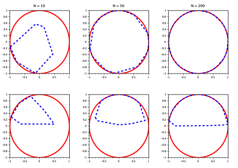
Figure 1. Row 1 (resp. 2): plots of $\widehat{C}_{N}$ computed from $N=10$, $50$ and $200$ observations of $X^{1}$ (resp. $X^{2}$).

On the other hand, $\widehat{C}_{N}$ has been computed from $100$ datasets of $N=200$ observations of $X^{1}$. The $100$-mean Hausdorff distance between $\widehat{C}_{200}$ and $C$ is small: 0.002 (with StD. 0.007).

Now, let us consider the previous model $X^{1}=\Pi_{C}(H^{1})$, but here with $C=[0,1]^{2}$. Again, $H^{1}$ fulfills the conditions (8) and (9) (with $r=m=2$), but also the conditions (6) and (7) in Proposition 3.1. Figure 2 illustrates the convergence of both $\widehat{C}_{N}$ and $\widetilde{C}_{N}$ for $N=10$, $50$ and $100$ observations of $X^{1}$. Clearly, $\widetilde{C}_{N}$ seems to converge faster to $C$ than $\widehat{C}_{N}$ as suggested by the theoretical results (see Propositions 3.1.(2) and 3.5).

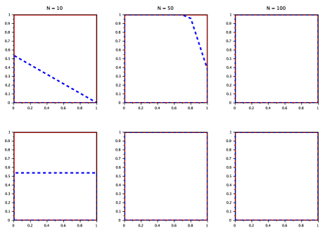
Figure 2. Row 1 (resp. 2): plots of $\widehat{C}_{N}$ (resp. $\widetilde{C}_{N}$) computed from $N=10$, $50$ and $100$ observations of $X$.

Finally, let us consider the following discrete-time Skorokhod problem

(17) $$\left\{\begin{array}[]{rcl}\overline{\tt X}_{j+1}&=&\Pi_{\texttt{C}(t_{j+1})}(\overline{\tt X}_{j}-\overline{\tt X}_{j}\Delta_{n}+10(\texttt{W}_{t_{j+1}}-\texttt{W}_{t_{j}}))\\ \overline{\tt X}_{0}&\equiv&1\in\texttt{C}(0)\end{array}\right.\textrm{$;$ }j\in J_{n}\backslash\{n\},$$

where $\Delta_{n}:=T/n$ with $T=5$ and $n=1000$, W is a $1$-dimensional Brownian motion, $\texttt{C}:[0,T]\rightrightarrows\mathbb{R}$ is the multifunction defined by

$$\texttt{C}(t):=\left[-(t-1)^{2}-\frac{1}{2},(t-1)^{2}+\frac{1}{2}\right]\textrm{ $;$ }\forall t\in[0,T],$$

$J_{n}:=\{0,\dots,n\}$, and $t_{j}:=j\Delta_{n}$ for every $j\in J_{n}$. The solution $\overline{\tt X}$ of Problem (17) approximates a (dynamically) reflected Ornstein-Uhlenbeck process. On the one hand, Figure 3 illustrates the convergence of $\widehat{\tt C}_{N,1},\dots,\widehat{\tt C}_{N,n}$ for $N=10$, $50$, $200$ and $500$ observations of $\overline{\tt X}$.

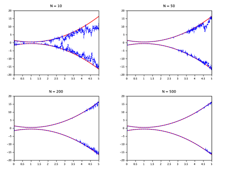
Figure 3. Plots of $j\mapsto\widehat{\tt C}_{N,j}$ for $N=10$, $50$, $200$ and $500$ observations of $\overline{\tt X}$.

On the other hand, $j\mapsto\widehat{\tt C}_{N,j}$ has been computed from $K=100$ datasets of $N=100$, $200$ and $300$ observations of $\overline{\tt X}$. For each value of $N$, the quality of the estimation of $\texttt{C}(\cdot)$ by $\widehat{\tt C}_{N,.}$ has been evaluated by computing the mean and the standard deviation of the observations of $d_{\rm H}(\widehat{\tt C}_{N,j}^{k},\texttt{C}(t_{j}))$ where, for every $k\in\{1,\dots,K\}$ and $j\in J_{n}\backslash\{0\}$, $\widehat{\tt C}_{N,j}^{k}$ is our estimator of $\texttt{C}(t_{j})$ computed from the $k$-th dataset. Table 1 shows that, as expected, the error of our estimator decreases (in mean and standard deviation) when $N$ grows.

$N$	Mean error	Error StD.
100	0.272	0.723
200	0.125	0.410
300	0.069	0.274

Table 1. Means and StD. of the error of $\widehat{\tt C}_{N,1},\dots,\widehat{\tt C}_{N,n}$ for $N=100$, $200$ and $300$ ($100$ repetitions).

Appendix A Proofs

A.1. Proof of Proposition 2.2

First, let us show that $H$ satisfies (4) if and only if

(18) $$\Phi((-\infty,S))\subset[0,1)\quad{\rm and}\quad\Phi((I,\infty))\subset(0,1].$$

On the one hand, if $H$ satisfies (18), then

$$\Phi((I,S)) = \Phi((-\infty,S)\cap(I,\infty))$$

$$\subset \Phi((-\infty,S))\cap\Phi((I,\infty))\subset[0,1)\cap(0,1]=(0,1).$$

On the other hand, (4) implies (18) because $\Phi$ is increasing. Now, let us prove that if

(19) $$\Phi((-\infty,S))\subset[0,1),$$

then $\widehat{S}_{N}$ is a converging estimator of $S$. By (19) and Lemma 2.1,

(20) $$\sup\{x\in\mathbb{R}:F(x)<1\}=S.$$

Let $F_{N}$ be the distribution function of $\widehat{S}_{N}$. Since $X_{1},\dots,X_{N}$ are independent copies of $X$, for any $x\in\mathbb{R}$,

$$F_{N}(x)=\mathbb{P}\left(\bigcap_{i=1}^{N}\{X_{i}\leqslant x\}\right)=F(x)^{N}.$$

On the one hand, for $x<S$, $F(x)\in[0,1)$ by (20), and then

$$\lim_{N\rightarrow\infty}F_{N}(x)=\lim_{N\rightarrow\infty}F(x)^{N}=0.$$

On the other hand, for $x\geqslant S$, $F(x)=1$ by (20), and then

$$\lim_{N\rightarrow\infty}F_{N}(x)=\lim_{N\rightarrow\infty}F(x)^{N}=1.$$

So, $F_{N}$ converges pointwise to $\mathbb{1}_{[S,\infty)}$ (the distribution function of $\omega\mapsto S$), leading to

$$\widehat{S}_{N}\xrightarrow[N\rightarrow\infty]{\mathbb{P}}S.$$

Finally, by assuming that $H$ satisfies (4) (or equivalently (18)),

$$\widehat{I}_{N}\xrightarrow[N\rightarrow\infty]{\mathbb{P}}I,$$

and thus

$$d_{\rm H}(\widehat{C}_{N},C) = \sup_{x\in C}d(x,\widehat{C}_{N})\quad{\rm because}\quad\widehat{C}_{N}\subset C$$

$$= \max\{|\widehat{S}_{N}-S|,|\widehat{I}_{N}-I|\}\xrightarrow[N\rightarrow\infty]{\mathbb{P}}0.$$

A.2. Proof of Proposition 2.3

First, since $X$ is a $[I,S]$-valued random variable, for every $x\in\mathbb{R}_{+}$,

$$\mathbb{P}(N(\widehat{S}_{N}-S)\leqslant x)=\mathbb{P}\left(X\leqslant S+\frac{x}{N}\right)^{N}=1.$$

Now, by Lemma 2.1, and by the definition of the left-sided derivative of $\Phi$ at point $S$, for every $y\in[I,S)$,

$$\mathbb{P}(X>y) = 1-F(y)$$

$$= 1-\Phi(y)\underset{y\uparrow S}{\sim}1-\Phi(S)-\Phi^{\prime}(S^{-})(y-S).$$

Then, for any $x<0$,

$$\mathbb{P}\left(X>S+\frac{x}{N}\right)\underset{N\rightarrow\infty}{\sim}1-\Phi(S)-\Phi^{\prime}(S^{-})\frac{x}{N},$$

leading to

$$\mathbb{P}(N(\widehat{S}_{N}-S)\leqslant x) = \left(1-\mathbb{P}\left(X>S+\frac{x}{N}\right)\right)^{N}$$

$$\underset{N\rightarrow\infty}{\sim} \left(\Phi(S)+\Phi^{\prime}(S^{-})\frac{x}{N}\right)^{N}\underset{N\rightarrow\infty}{\sim}\Phi(S)^{N}\exp\left(-\left|\frac{\delta x}{\Phi(S)}\right|\right).$$

Therefore,

1. If $\Phi(S)<1$, then the distribution function of $N(\widehat{S}_{N}-S)$ converges pointwise to $\mathbb{1}_{\mathbb{R}_{+}}$. In other words,

   $$N(\widehat{S}_{N}-S)\xrightarrow[N\rightarrow\infty]{\mathbb{P}}0.$$

2. If $\Phi(S)=1$ and $\delta\neq 0$, then the distribution function of $N\delta(\widehat{S}_{N}-S)$ converges pointwise to $e^{-|\cdot|}\mathbb{1}_{(-\infty,0)}(\cdot)+\mathbb{1}_{\mathbb{R}_{+}}(\cdot)$. In other words,

   $$N\delta(\widehat{S}_{N}-S)\xrightarrow[N\rightarrow\infty]{\mathcal{D}}{\rm Weibull}(1).$$

A.3. Proof of Proposition 3.4

First, assume that $H$ satisfies (8). On the one hand, for any $y\in(I,S)={\rm int}(C)$,

$$\Phi(y) = \mathbb{P}_{H}((-\infty,y])$$

$$= \mathbb{P}_{H}((-\infty,I])$$

$$\hskip 28.45274pt+\mathbb{P}_{H}((I,y-\eta])$$

$$\hskip 56.9055pt+\mathbb{P}_{H}((y-\eta,y])\quad{\rm with}\quad\eta\in(0,y-I)$$

$$= R(y,\eta)+\mathbb{P}_{H}([x-\varepsilon,x+\varepsilon]\cap(I,S)),$$

where

$$R(y,\eta):=\mathbb{P}_{H}((-\infty,I])+\mathbb{P}_{H}((y-\eta,y]),$$

$$\hskip 42.67912ptx:=\frac{I+y-\eta}{2}\in(I,y-\eta)\subset{\rm int}(C)\quad{\rm and}\quad\varepsilon:=\frac{y-\eta-I}{2}>0.$$

Then, $\Phi(y)>0$ by (8), and since $y$ has been arbitrarily chosen in $(I,S)$,

$$\Phi((I,S))\subset(0,1].$$

On the other hand, for any $y\in(I,S)={\rm int}(C)$,

$$\Phi(y) = 1-\mathbb{P}_{H}((y,\infty))$$

$$= 1-\mathbb{P}_{H}((y,y+\eta))$$

$$\hskip 28.45274pt-\mathbb{P}_{H}([y+\eta,S))$$

$$\hskip 56.9055pt-\mathbb{P}_{H}([S,\infty))\quad{\rm with}\quad\eta\in(0,S-y)$$

$$= 1-R(y,\eta)-\mathbb{P}_{H}([x-\varepsilon,x+\varepsilon]\cap(I,S)),$$

where

$$R(y,\eta):=\mathbb{P}_{H}((y,y+\eta))+\mathbb{P}_{H}([S,\infty)),$$

$$\hskip 42.67912ptx:=\frac{y+\eta+S}{2}\in(y+\eta,S)\subset{\rm int}(C)\quad{\rm and}\quad\varepsilon:=\frac{S-y-\eta}{2}>0.$$

Then, $\Phi(y)<1$ by (8), and since $y$ has been arbitrarily chosen in $(I,S)$,

$$\Phi((I,S))\subset[0,1).$$

Therefore, $H$ satisfies (4) as expected. Now, assume that $H$ satisfies (4), and that $\Phi$ is strictly increasing on $(I,S)$. For every $x\in{\rm int}(C)=(I,S)$ and $\varepsilon>0$,

$$\mathbb{P}_{H}([x-\varepsilon,x+\varepsilon]\cap(I,S)) \geqslant \mathbb{P}(I\vee(x-\varepsilon)<H<S\wedge(x+\varepsilon))$$

$$= \Phi((S\wedge(x+\varepsilon))^{-})-\Phi(I\vee(x-\varepsilon))>0.$$

Therefore, $H$ satisfies (8).

A.4. Proof of Proposition 3.8

Let $(C_{n})_{n\in\mathbb{N}^{*}}$ be a sequence of convex-compact polyhedra of $\mathbb{R}^{m}$, such that the set $\mathcal{V}_{n}$ of the vertices of $C_{n}$ satisfies $|\mathcal{V}_{n}|=n$ and $\mathcal{V}_{n}\subset C$ for every $n\in\mathbb{N}^{*}$, and such that

(21) $$\lim_{n\rightarrow\infty}n^{\frac{1}{r}}d_{\rm H}(C_{n},C)=0.$$

Such a sequence exists by Kamenev [10], Theorem 2. For any $\kappa\in(0,1/r)$, $\varepsilon>0$ and $n\in\mathbb{N}^{*}$, as in the proof of Proposition 3.7,

$$\left\{N^{\frac{1}{r}-\kappa}d_{\rm H}(\widehat{C}_{N},C_{n})>\frac{\varepsilon}{2}\right\}$$

$$\hskip 56.9055pt\subset\left\{\sup\{d(\mathbf{v},\widehat{C}_{N})\textrm{ $;$ }\mathbf{v}\in\mathcal{V}_{n}\}>\frac{\varepsilon}{2}N^{\kappa-\frac{1}{r}}\right\}$$

$$\hskip 113.81102pt\cup\left\{d_{\rm H}(C_{n},C)=\sup\{d(\mathbf{x},C_{n})\textrm{ $;$ }\mathbf{x}\in C\}>\frac{\varepsilon}{2}N^{\kappa-\frac{1}{r}}\right\}$$

and then, by (15),

$$\mathbb{P}(N^{\frac{1}{r}-\kappa}d_{\rm H}(\widehat{C}_{N},C)>\varepsilon) \leqslant \sum_{\mathbf{v}\in\mathcal{V}_{n}}\mathbb{P}\left(d(\mathbf{v},\widehat{C}_{N})>\frac{\varepsilon}{2}N^{\kappa-\frac{1}{r}}\right)+2\mathbb{1}_{d_{\rm H}(C_{n},C)>\frac{\varepsilon}{2}N^{\kappa-\frac{1}{r}}}$$

$$\leqslant n\left(1-\varphi\left(\frac{\varepsilon}{2}N^{\kappa-\frac{1}{r}}\right)\right)^{N}+2\mathbb{1}_{n^{\frac{1}{r}}d_{\rm H}(C_{n},C)>\frac{\varepsilon}{2}n^{\frac{1}{r}}N^{\kappa-\frac{1}{r}}}.$$

Moreover, by (15),

$$N\left(1-\varphi\left(\frac{\varepsilon}{2}N^{\kappa-\frac{1}{r}}\right)\right)^{N}\underset{N\rightarrow\infty}{\sim}N\exp\left(-\mathfrak{c}\left(\frac{\varepsilon}{2}\right)^{r}N^{\kappa r}\right)\xrightarrow[N\rightarrow\infty]{}0,$$

and by (21),

$$\lim_{N\rightarrow\infty}\mathbb{1}_{N^{\frac{1}{r}-\kappa}d_{\rm H}(C_{N},C)>\frac{\varepsilon}{2}}=0.$$

Therefore, for $n=N$,

$$\mathbb{P}(N^{\frac{1}{r}-\kappa}d_{\rm H}(\widehat{C}_{N},C)>\varepsilon)$$

$$\hskip 42.67912pt\leqslant N\left(1-\varphi\left(\frac{\varepsilon}{2}N^{\kappa-\frac{1}{r}}\right)\right)^{N}+2\mathbb{1}_{N^{\frac{1}{r}-\kappa}d_{\rm H}(C_{N},C)>\frac{\varepsilon}{2}}\xrightarrow[N\rightarrow\infty]{}0.$$

A.5. Proof of Proposition 4.2

For every $j\in J_{n}\backslash\{n\}$, consider

$$\texttt{H}_{j+1}:=\overline{\tt X}_{j}+b(\overline{\tt X}_{j})\Delta_{n}+\sigma(\overline{\tt X}_{j})\texttt{Z}_{j+1}\quad{\rm with}\quad\texttt{Z}_{j+1}=\texttt{W}_{t_{j+1}}-\texttt{W}_{t_{j}}.$$

The proof of Proposition 4.2 is dissected in three steps. Step 1 deals with a suitable control of $\|\texttt{H}_{j+1}-\mathbf{x}\|$, depending on $\texttt{Z}_{j+1}$ and $\|\overline{\tt X}_{j}-\mathbf{x}\|$, for every $j\in J_{n}\backslash\{n\}$ and $\mathbf{x}\in\texttt{C}(t_{j+1})$. In Step 2, the condition

$$\mathbb{P}_{\texttt{H}_{j}}(\overline{B}_{d}(\mathbf{x},\varepsilon)\cap{\rm int}(\texttt{C}(t_{j})))>0\textrm{ $;$}$$

$$\hskip 85.35826pt\forall j\in J_{n}\backslash\{0\}\textrm{, }\forall\varepsilon>0\textrm{, }\forall\mathbf{x}\in{\rm int}(\texttt{C}(t_{j}))$$

is checked in order to apply Proposition 3.3 to $\widehat{\tt C}_{N,1},\dots,\widehat{\tt C}_{N,n}$ in Step 3.

Step 1. For any $j\in J_{n}\backslash\{n\}$ and $\mathbf{x}\in\texttt{C}(t_{j+1})$, since $b$ and $\sigma$ are Lipschitz continuous maps,

$$\|\texttt{H}_{j+1}-\mathbf{x}\| = \|\overline{\tt X}_{j}-\mathbf{x}+(b(\overline{\tt X}_{j})-b(\mathbf{x}))\Delta_{n}$$

$$\hskip 56.9055pt+(\sigma(\overline{\tt X}_{j})-\sigma(\mathbf{x}))\texttt{Z}_{j+1}+b(\mathbf{x})\Delta_{n}+\sigma(\mathbf{x})\texttt{Z}_{j+1}\|$$

$$\leqslant (1+\|b\|_{\rm Lip}\Delta_{n}+\|\sigma\|_{\rm Lip}\|\texttt{Z}_{j+1}\|)\|\overline{\tt X}_{j}-\mathbf{x}\|+\texttt{R}_{j+1}(\mathbf{x})$$

$$\hskip 113.81102pt{\rm with}\quad\texttt{R}_{j+1}(\mathbf{x})=\|\sigma(\mathbf{x})\texttt{Z}_{j+1}+b(\mathbf{x})\Delta_{n}\|.$$

On the one hand, since $\sigma(\mathbf{x})\in{\rm GL}_{m}(\mathbb{R})$,

$$\|\texttt{Z}_{j+1}\| = \|\sigma(\mathbf{x})^{-1}(\sigma(\mathbf{x})\texttt{Z}_{j+1}+b(\mathbf{x})\Delta_{n}-b(\mathbf{x})\Delta_{n})\|$$

$$\leqslant \|\sigma(\mathbf{x})^{-1}\|_{\rm op}(\texttt{R}_{j+1}(\mathbf{x})+\|b(\mathbf{x})\|\Delta_{n}).$$

On the other hand, since $\texttt{C}(t_{0}),\dots,\texttt{C}(t_{n})\subset\texttt{C}(0)$, and since $\texttt{C}(0)$ is a compact subset of $\mathbb{R}^{m}$, there exists a constant $\mathfrak{m}_{\tt C}>0$ such that, for every $k\in J_{n}$ and $\mathbf{v}\in\texttt{C}(t_{k})$, $\|\mathbf{v}\|\leqslant\mathfrak{m}_{\tt C}$. Thus,

(22) $$\|\texttt{H}_{j+1}-\mathbf{x}\|\leqslant\mathfrak{c}_{1}\|\overline{\tt X}_{j}-\mathbf{x}\|+\mathfrak{c}_{2}\texttt{R}_{j+1}(\mathbf{x})$$

with

$$\mathfrak{c}_{1} = 1+\left(\|b\|_{\rm Lip}+\|\sigma\|_{\rm Lip}\sup_{\|\mathbf{v}\|\leqslant\mathfrak{m}_{\tt C}}\{\|\sigma(\mathbf{v})^{-1}\|_{\rm op}\|b(\mathbf{v})\|\}\right)\Delta_{n}$$

$$\hskip 113.81102pt{\rm and}\quad\mathfrak{c}_{2}=1+2\mathfrak{m}_{\tt C}\|\sigma\|_{\rm Lip}\sup_{\|\mathbf{v}\|\leqslant\mathfrak{m}_{\tt C}}\|\sigma(\mathbf{v})^{-1}\|_{\rm op}.$$

Step 2. For every $j\in J_{n}\backslash\{0\}$ and $\mathbf{x}\in{\rm int}(\texttt{C}(t_{j}))$, there exists $\varepsilon_{j,\mathbf{x}}>0$ such that

(23) $$\overline{B}_{d}(\mathbf{x},\varepsilon_{j,\mathbf{x}})\subset{\rm int}(\texttt{C}(t_{j})).$$

First, for every $\varepsilon>0$ and $\mathbf{x}\in{\rm int}(\texttt{C}(t_{1}))$, by (23), since $\sigma(\mathbf{x}_{0})\in{\rm GL}_{m}(\mathbb{R})$, and since $[\texttt{W}_{t_{1}}]_{1},\dots,[\texttt{W}_{t_{1}}]_{m}$ are i.i.d. Gaussian random variables,

$$\mathbb{P}_{\texttt{H}_{1}}(\overline{B}_{d}(\mathbf{x},\varepsilon)\cap{\rm int}(\texttt{C}(t_{1})))$$

$$\hskip 28.45274pt\geqslant\mathbb{P}(\|\mathbf{x}_{0}-\mathbf{x}+b(\mathbf{x}_{0})\Delta_{n}+\sigma(\mathbf{x}_{0})\texttt{W}_{t_{1}}\|\leqslant\varepsilon\wedge\varepsilon_{1,\mathbf{x}})$$

$$\hskip 28.45274pt\geqslant\mathbb{P}(\|\texttt{W}_{t_{1}}+\sigma(\mathbf{x}_{0})^{-1}(\mathbf{x}_{0}-\mathbf{x}+b(\mathbf{x}_{0})\Delta_{n})\|\leqslant\|\sigma(\mathbf{x}_{0})\|_{\rm op}^{-1}(\varepsilon\wedge\varepsilon_{1,\mathbf{x}}))\geqslant\mu_{1,\mathbf{x}}(\varepsilon)$$

with

$$\mu_{1,\mathbf{x}}(\varepsilon) = \prod_{k=1}^{m}\mathbb{P}(|[\texttt{W}_{t_{1}}]_{k}+[\sigma(\mathbf{x}_{0})^{-1}(\mathbf{x}_{0}-\mathbf{x}+b(\mathbf{x}_{0})\Delta_{n})]_{k}|$$

$$\hskip 142.26378pt\leqslant(\sqrt{m}\|\sigma(\mathbf{x}_{0})\|_{\rm op})^{-1}(\varepsilon\wedge\varepsilon_{1,\mathbf{x}}))>0.$$

Now, consider $j\in J_{n}\backslash\{0,n\}$, and assume that for every $\varepsilon>0$ and $\mathbf{x}\in{\rm int}(\texttt{C}(t_{j}))$,

(24) $$\mathbb{P}_{\texttt{H}_{j}}(\overline{B}_{d}(\mathbf{x},\varepsilon)\cap{\rm int}(\texttt{C}(t_{j})))>0.$$

For any $\varepsilon>0$ and $\mathbf{x}\in{\rm int}(\texttt{C}(t_{j+1}))$, by Inequality (22), by (23), since $\texttt{Z}_{j+1}$ (and then $\texttt{R}_{j+1}$) is independent of $\mathcal{F}_{j}=\sigma(\texttt{W}_{t_{0}},\dots,\texttt{W}_{t_{j}})$, and since $\overline{\tt X}_{j}$ is $\mathcal{F}_{j}$-measurable,

$$\mathbb{P}_{\texttt{H}_{j+1}}(\overline{B}_{d}(\mathbf{x},\varepsilon)\cap{\rm int}(\texttt{C}(t_{j+1})))$$

$$\hskip 42.67912pt\geqslant\mathbb{P}(\|\texttt{H}_{j+1}-\mathbf{x}\|\leqslant\varepsilon\wedge\varepsilon_{j+1,\mathbf{x}})$$

$$\hskip 42.67912pt\geqslant\mathbb{P}(\mathfrak{c}_{1}\|\overline{\tt X}_{j}-\mathbf{x}\|\leqslant 2^{-1}(\varepsilon\wedge\varepsilon_{j+1,\mathbf{x}}),\mathfrak{c}_{2}\texttt{R}_{j+1}(\mathbf{x})\leqslant 2^{-1}(\varepsilon\wedge\varepsilon_{j+1,\mathbf{x}}))$$

$$\hskip 42.67912pt\geqslant\mathbb{P}(\|\overline{\tt X}_{j}-\mathbf{x}\|\leqslant(2\mathfrak{c}_{1})^{-1}(\varepsilon\wedge\varepsilon_{j+1,\mathbf{x}}),\texttt{H}_{j}\in{\rm int}(\texttt{C}(t_{j})))$$

$$\hskip 184.9429pt\times\mathbb{P}(\texttt{R}_{j+1}(\mathbf{x})\leqslant(2\mathfrak{c}_{2})^{-1}(\varepsilon\wedge\varepsilon_{j+1,\mathbf{x}})).$$

On the one hand, since $\overline{\tt X}_{j}=\texttt{H}_{j}$ on $\{\texttt{H}_{j}\in{\rm int}(\texttt{C}(t_{j}))\}$, and since $\texttt{C}(t_{j+1})\subset\texttt{C}(t_{j})$, by (24),

$$\mathbb{P}(\|\overline{\tt X}_{j}-\mathbf{x}\|\leqslant(2\mathfrak{c}_{1})^{-1}(\varepsilon\wedge\varepsilon_{j+1,\mathbf{x}}),\texttt{H}_{j}\in{\rm int}(\texttt{C}(t_{j})))$$

$$\hskip 113.81102pt=\mathbb{P}_{\texttt{H}_{j}}(\overline{B}_{d}(\mathbf{x},(2\mathfrak{c}_{1})^{-1}(\varepsilon\wedge\varepsilon_{j+1,\mathbf{x}}))\cap{\rm int}(\texttt{C}(t_{j})))>0.$$

On the other hand, since $\sigma(\mathbf{x})\in{\rm GL}_{m}(\mathbb{R})$, and since $[\texttt{Z}_{j+1}]_{1},\dots,[\texttt{Z}_{j+1}]_{m}$ are i.i.d. Gaussian random variables,

$$\mathbb{P}(\texttt{R}_{j+1}(\mathbf{x})\leqslant(2\mathfrak{c}_{2})^{-1}(\varepsilon\wedge\varepsilon_{j+1,\mathbf{x}}))$$

$$\hskip 28.45274pt\geqslant\mathbb{P}(\|\sigma(\mathbf{x})\|_{\rm op}\|\texttt{Z}_{j+1}+\sigma(\mathbf{x})^{-1}b(\mathbf{x})\Delta_{n}\|\leqslant(2\mathfrak{c}_{2})^{-1}(\varepsilon\wedge\varepsilon_{j+1,\mathbf{x}}))\geqslant\mu_{j+1,\mathbf{x}}(\varepsilon)$$

with

$$\mu_{j+1,\mathbf{x}}(\varepsilon) = \prod_{k=1}^{m}\mathbb{P}(|[\texttt{Z}_{j+1}]_{k}+[\sigma(\mathbf{x})^{-1}b(\mathbf{x})]_{k}\Delta_{n}|$$

$$\hskip 99.58464pt\leqslant(2\mathfrak{c}_{2}\sqrt{m}\|\sigma(\mathbf{x})\|_{\rm op})^{-1}(\varepsilon\wedge\varepsilon_{j+1,\mathbf{x}}))>0.$$

Step 3 (conclusion). By Step 2, for any $j\in J_{n}\backslash\{0\}$,

$$\mathbb{P}_{\texttt{H}_{j}}(\overline{B}_{d}(\mathbf{x},\varepsilon)\cap{\rm int}(\texttt{C}(t_{j})))>0\textrm{ $;$ }\forall\varepsilon>0\textrm{, }\forall\mathbf{x}\in{\rm int}(\texttt{C}(t_{j})).$$

Thus, by Proposition 3.3, $\widehat{\tt C}_{N,j}$ converges pointwise to $\texttt{C}(t_{j})$:

$$d(\mathbf{x},\widehat{\tt C}_{N,j})\xrightarrow[N\rightarrow\infty]{\mathbb{P}}0\textrm{ $;$ }\forall\mathbf{x}\in{\rm int}(\texttt{C}(t_{j})).$$

A.6. Proof of Proposition 4.3

For any $\mathbf{x}\in{\rm int}(\texttt{K})$, there exists $\varepsilon_{\mathbf{x}}>0$ such that

$$\overline{B}_{d}(\mathbf{x},\varepsilon_{\bf x})\subset{\rm int}(\texttt{K}).$$

Then, since $\sigma(\mathbf{x}_{0})\in{\rm GL}_{m}(\mathbb{R})$, and since $[\texttt{W}_{t_{1}}]_{1},\dots,[\texttt{W}_{t_{1}}]_{m}$ are independent random variables,

$$\mathbb{P}_{\texttt{H}_{1}}(\overline{B}_{d}(\mathbf{x},\varepsilon)\cap{\rm int}(\texttt{K}))$$

$$\hskip 28.45274pt\geqslant\mathbb{P}(\|\mathbf{x}_{0}-\mathbf{x}+b(\mathbf{x}_{0})\Delta_{n}+\sigma(\mathbf{x}_{0})\texttt{W}_{t_{1}}\|\leqslant\varepsilon\wedge\varepsilon_{\bf x})$$

$$\hskip 28.45274pt\geqslant\mathbb{P}(\|\texttt{W}_{t_{1}}+\sigma(\mathbf{x}_{0})^{-1}(\mathbf{x}_{0}-\mathbf{x}+b(\mathbf{x}_{0})\Delta_{n})\|\leqslant\|\sigma(\mathbf{x}_{0})\|_{\rm op}^{-1}(\varepsilon\wedge\varepsilon_{1,\mathbf{x}}))\geqslant\mu_{\bf x}(\varepsilon),$$

where

$$\mu_{\bf x}(\varepsilon) := \prod_{k=1}^{m}\mathbb{P}(|[\texttt{W}_{t_{1}}]_{k}+[\sigma(\mathbf{x}_{0})^{-1}(\mathbf{x}_{0}-\mathbf{x}+b(\mathbf{x}_{0})\Delta_{n})]_{k}|$$

$$\hskip 142.26378pt\leqslant(\sqrt{m}\|\sigma(\mathbf{x}_{0})\|_{\rm op})^{-1}(\varepsilon\wedge\varepsilon_{\bf x}))$$

$$= \prod_{k=1}^{m}\mathbb{P}([\texttt{W}_{t_{1}}]_{k}\in[\mathfrak{c}_{\mathbf{x},k}\pm\mathfrak{s}(\varepsilon\wedge\varepsilon_{\bf x})])$$

with

$$\mathfrak{c}_{\mathbf{x},.}=-\sigma(\mathbf{x}_{0})^{-1}(\mathbf{x}_{0}-\mathbf{x}+b(\mathbf{x}_{0})\Delta_{n})\quad{\rm and}\quad\mathfrak{s}=(\sqrt{m}\|\sigma(\mathbf{x}_{0})\|_{\rm op})^{-1}.$$

Let $f$ be the common Gaussian density function of $[\texttt{W}_{t_{1}}]_{1},\dots,[\texttt{W}_{t_{1}}]_{m}$. Since $f(\cdot)>0$ on $\mathbb{R}$,

$$\mathbb{P}_{\texttt{H}_{1}}(\overline{B}_{d}(\mathbf{x},\varepsilon)\cap{\rm int}(\texttt{K})) \geqslant \prod_{k=1}^{m}\int_{-\mathfrak{s}(\varepsilon\wedge\varepsilon_{\bf x})}^{\mathfrak{s}(\varepsilon\wedge\varepsilon_{\bf x})}f(\mathfrak{c}_{\mathbf{x},k}+x)dx$$

$$= (\varepsilon\wedge\varepsilon_{\mathbf{x}})^{m}\prod_{k=1}^{m}\int_{-\mathfrak{s}}^{\mathfrak{s}}f(\mathfrak{c}_{\mathbf{x},k}+(\varepsilon\wedge\varepsilon_{\mathbf{x}})y)dy$$

$$\geqslant \varphi_{\bf x}(\varepsilon):=(\varepsilon\wedge\varepsilon_{\mathbf{x}})^{m}\underbrace{(2\mathfrak{s})^{m}\prod_{k=1}^{m}\min\{f(y)\textrm{ $;$ }y\in[\mathfrak{c}_{\mathbf{x},k}\pm\varepsilon_{\bf x}\mathfrak{s}]\}}_{=:\mathfrak{c}_{\bf x}}.$$

So, since

$$\varphi_{\bf x}(\varepsilon)\underset{\varepsilon\downarrow 0}{\sim}\mathfrak{c}_{\bf x}\varepsilon^{m},$$

the random variable $\texttt{H}_{1}$ fulfills the condition (9) in Proposition 3.5 with $r=m$. In conclusion, for every $\kappa\in(0,1/m)$ and $\mathbf{x}\in{\rm int}({\tt K})$,

$$N^{\frac{1}{m}-\kappa}d(\mathbf{x},\widehat{\tt C}_{N,1})\xrightarrow[N\rightarrow\infty]{\mathbb{P}}0.$$

References

- [1] Bernicot, F. and Venel, J. (2011). Stochastic Perturbation of Sweeping Process and a Convergence Result for an Associated Numerical Scheme. Journal of Differential Equations 251, 1195-1224.
- [2] Brunel, V-E. (2018). Methods for Estimation of Convex Sets. Statistical Science 33(4), 615-632.
- [3] Brunel, V-E. (2019). Uniform Behaviors of Random Polytopes Under the Hausdorff Metric. Bernoulli 25(3), 1770-1793.
- [4] Casal, A.R. (2007). Set Estimation Under Convexity Type Assumptions. Annales de l’IHP B 43(6), 763-774.
- [5] Cattiaux, P., León, J.R. and Prieur, C. (2017). Invariant Density Estimation for Reflected Diffusion Using An Euler Scheme. Monte Carlo Methods and Applications 23(2), 71-88.
- [6] Comte, F. and Genon-Catalot, V. (2020). Nonparametric Drift Estimation for I.I.D. Paths of Stochastic Differential Equations. The Annals of Statistics 48, 6, 3336-3365.
- [7] Cuevas, A. (2009). Set Estimation: Another Bridge Between Statistics and Geometry. Boletín de Estadística e Investigación Operativa 25(2), 71-85.
- [8] Denis, C., Dion-Blanc, C. and Martinez, M. (2021). A Ridge Estimator of the Drift from Discrete Repeated Observations of the Solution of a Stochastic Differential Equation. Bernoulli 27, 2675-2713.
- [9] Dümbgen, L. and Walther, G. (1996). Rates of Convergence for Random Approximations of Convex Sets. Advances in Applied Probability 28(2), 384-393.
- [10] Kamenev, G.K. (1992). A Class of Adaptive Algorithms for Approximating Convex Bodies by Polyhedra. Computational Mathematics and Mathematical Physics 32(1), 114-127.
- [11] Marie, N. and Rosier, A. (2023). Nadaraya-Watson Estimator for I.I.D. Paths of Diffusion Processes. Scandinavian Journal of Statistics 50, 2, 589-637.
- [12] Rockafellar, R.T. (1997). Convex Analysis. Princeton University Press.