Cost and Power-Consumption Analysis for Power Profile Monitoring with Multiple Monitors per Link in Optical Networks

Abstract

Network monitoring is essential to collect comprehensive data on signal quality in optical networks. As deploying large amounts of monitoring equipment results in elevated cost and power consumption, novel low-cost monitoring methods are continuously being investigated. A new technique called Power Profile Monitoring (PPM) has recently gained traction thanks to its ability to monitor an entire lightpath using a single post-processing unit at the lightpath receiver. PPM does not require to deploy an individual monitor for each span, as in the traditional monitoring technique using Optical Time-Domain Reflectometer (OTDR). PPM and OTDR have different monitoring applications, which will be elaborated in our discussion, hence they can be considered either alternative or complementary techniques according to the targeted monitoring capabilities to be implemented in the network. In this work, we aim to quantify the cost and power consumption of PPM (using OTDR as a baseline reference), as this analysis can provide guidelines for the implementation and deployment of PPM. First, we discuss how PPM and OTDR monitors are deployed, and we formally state a new Optimized Monitoring Placement (OMP) problem for PPM. Solving the OMP problem allows to identify the minimum number of PPM monitors that guarantees that all links in the networks are monitored by at least $n$ PPM monitors (note that using $n>1$ allows for increased monitoring accuracy). We prove the NP-hardness of the OMP problem and formulate it using an Integer Linear Programming (ILP) model. Finally, we also devise a heuristic algorithm for the OMP problem to scale to larger topologies. Our numerical results, obtained on realistic topologies, suggest that the cost (power) of one PPM module should be lower than 2.6 times and 10.2 times that of one OTDR for nation-wide and continental-wide topology, respectively.

I Introduction

For several critical management tasks in optical networks, monitoring equipment is essential to collect comprehensive data on impairments affecting optical transmissions and components. Leveraging data collected by monitors, we can reduce optical margins, detect anomalies for troubleshooting, and ultimately optimize the system performance [1, 2]. Among all the monitored parameters, power has the most significant impact, as it can be used for identifying and localizing power losses, for tracking changes/splices, for fiber characterization, etc. Traditional monitoring techniques mainly retrieve the power using Optical Channel Monitors (OCMs) [1, 2] and Optical Time-Domain Reflectometers (OTDRs) [3]. OCM is typically used to measure the power after amplification in amplifiers, but it cannot be used to obtain the power at each point of the optical line [1]. Instead, OTDR injects an out-of-band signal to the optical line and is able to estimate the power of the injected signal at each point of the optical line to detect the anomalies in the optical line [4]. OTDR’s fine power monitoring capability is achieved at the expense of a considerable cost and power consumption, as one OTDR per amplifier is required to monitor the optical line unless additional optical components (such as Loop-Back Line Monitoring System) [5] are deployed. Hence, research is ongoing to devise novel low-cost monitoring methods [6, 7, 8]. One of these novel and potentially low-cost methods is the Power Profile Monitoring (PPM), which is currently attracting increasing attention [9, 10, 8]. PPM monitors the entire lightpath (LP) by using only an additional post-processing monitoring component at the receiver and, hence, it does not require monitoring each amplifier along the optical line as in traditional monitoring with OTDR [3].

The performance of PPM has been significantly improved in the last few years. First, the maximum error on loss has been reduced to 0.25 dB [11], which is comparable to that of OTDR (less than 0.5 dB) [12]. Second, the spatial resolution (i.e., minimum distance over which two consecutive power events can be distinguished) of PPM has been reduced to 500 meters with measurement distance up to 1200 km [13], while the spatial resolution of OTDR is hundreds of meters with a measurement distance of only 80 km [12]. The spatial resolution of OTDR can be reduced with a smaller pulse width, but this may result in decreased measurement distance [14]. In addition, the measurement distance of PPM has been extended to 10,000 kilometers [8], while the state-of-the-art record of measurement distance of OTDR is up to 28,000 kilometers [5]. Moreover, to address performance concerns of PPM related to insufficient performance of an LP (due to accumulated noise, such as amplified spontaneous emission or self-phase modulation noises) and an inaccurate transmission distance, Ref. [15] experimentally demonstrated improving monitoring accuracy by combining estimation from several LPs.

Following recent PPM experimental trials [8, 11, 13], PPM has confirmed its potential for several monitoring applications, especially considering the limited deployments of OTDR that are often installed only on selected links (especially in backbone networks). Hence, PPM is emerging as a cost-effective and power-efficient monitoring solution supporting various monitoring applications. Since PPM and OTDR have both shared and distinct monitoring applications, they can be considered either alternative or complementary techniques according to the targeted monitoring capabilities and budgetary constraints. Given this dual role of PPM, it becomes important to quantify the cost and power consumption of PPM on the network scale, which can be compared to that of OTDR as a baseline reference.

PPM technology is still evolving, and its implementation (and hence its cost and power consumption) is not yet defined. Thus, in this study, we provide a sensitivity analysis of its cost and power consumption to be used as a guideline for incoming implementations. Considering the ongoing debate on whether PPM should be integrated as a separate module or as a submodule within the receiver, we further evaluate the additional costs and power consumption added to the receiver when integrating PPM into the receiver. Our analysis compares the impact of different network architectures, namely, opaque vs. transparent “IP over Wavelength Division Multiplexing” (IPoWDM) network architectures [16]. Specifically, in transparent architecture, one LP may traverse several links instead of only one link, as in opaque architecture, leading to less required PPMs. Moreover, we evaluate the cost and power consumption required to improve monitoring accuracy using PPM on several LPs.

This is an extended version of our previous work in [17]. The main contributions and the difference of this work compared to [17] are as follows.

• We are the first, to the best of our knowledge, to investigate the problem of optimized monitoring placement (OMP) and quantitatively compare the cost and power consumption of PPM and OTDR. Compared to [17], we extend the OMP problem from only one monitor per link to multiple monitors per link.

• We prove the NP-hardness of the OMP problem and formulated an Integer Linear Programming (ILP) model for it. Moreover, to address the scalability issue of ILP, we propose an efficient heuristic algorithm that can optimize the placement of monitoring components.

• We provide extensive illustrative numerical evaluations to compare the cost and power consumption of PPM to OTDR. This evaluation provides guidelines for a network-wide deployment of PPM that is more cost-effective and energy-efficient than OTDR. These results of PPM are compared to a more resource-efficient deployment approach for OTDR compared to [17], to provide a more compelling baseline.

The remainder of the paper is organized as follows: Sec. II first illustrates the deployment of PPM and OTDR for network monitoring and then provides a formal problem statement for optimized monitoring placement. Sec. III describes our proposed optimized monitoring placement algorithm. Sec. IV presents and discusses the numerical results, comparing PPM to OTDR. Finally, Sec. V concludes the paper and indicates future work.

II System Model for Network Monitoring using PPM and OTDR

II-A Application Scenarios of PPM and OTDR

A comparison of the application scenarios for OTDR and PPM can be found in Table I. Both OTDR and PPM share some critical applications, such as optical loss detection and fiber characterization, owing to some foundational similarities in their working principles. Specifically, the applications of OTDR and PPM are both based on analyzing the power profile of monitoring signals (i.e., the injected signal and existing signal in LPs for OTDR and PPM, respectively).

TABLE I: Application Comparison between OTDR and PPM.

Application scenarios	OTDR	PPM
Monitoring of change in optical loss	Available	Available
Monitoring of fiber aging/splices	Available	Available
Monitoring of connecter loss	Available	Available
Fiber characterization	Available	Available
Monitoring of amplifiers (gain and possible anomalies)	Not available	Available
Monitoring of anomaly filters with a detuned center frequency	Not available	Available
Distributed optical power monitoring per wavelength	Not available	Available
Span-wise chromatic dispersion (CD) map estimation	Not available	Available
Monitoring of polarization-dependent loss	Not available	Available
Multi-path interference	Not available	Available
Localization of fiber cut	Available	Not available
Fiber quality assessment before the system is up	Available	Not available

Despite these similarities, PPM and OTDR also cater to distinct application scenarios. Specifically, as PPM can estimate the power in the entire LP, PPM can be used to monitor network devices (for example, monitoring the anomaly of amplifiers and the anomaly of filters with a detuned center frequency) [18]. Moreover, since PPM can estimate the power of the LP rather than the injected out-of-band signal as in OTDR, PPM can monitor LP such as span-wise chromatic dispersion (CD) map estimation [18], distributed optical power monitoring per wavelength [19], monitoring of polarization-dependent loss [20], multi-path interference [21], etc.

Conversely, OTDR supports applications not supported by PPM. Specifically, OTDR can localize fiber cut, while PPM cannot, since no signal is received in the receiver in case of fiber cut. Similarly, OTDR can diagnose fiber quality before the system is up and running by injecting signal, while PPM cannot unless generating test traffic through transponders.

This work does not aim to replace OTDR with PPM in those application scenarios that can not be covered by PPM (e.g., localization of fiber cut). Instead, if the operators want other monitoring capabilities not covered by OTDR using PPM, our work provides a baseline for evaluating the cost and power consumption of deploying PPM as a complementary monitoring technique. In addition, as a secondary scenario, for networks without OTDR (less likely scenario), when real-time fiber cut localization is not mandatory (note that the localization of links with fiber cut can be determined without deploying OTDR as in Ref. [22]), PPM can still offer an alternative to OTDR based on the applications (such as detecting change in optical loss, fiber aging, connector loss, etc.) that are most in the interest of the operator, and that can be provided by PPM.

II-B Implementation Options of PPM

The three main options for PPM implementation are (i) as a separate module outside the receiver, (ii) as a submodule inside the receiver, or (iii) through offline processing in servers. While offline server processing eliminates the need for additional hardware and hence has the lowest management cost, it does not support real-time processing and is typically implemented by sending data samples in batches over specified time intervals. Moreover, it incurs high telemetry costs for continuously transmitting data to the server. This study focuses on analyzing the extra cost and power consumption associated with enabling real-time monitoring with PPM, which is relevant to the first two implementation options. For the case of a separate module outside the receiver, the key advantage is its flexibility, as this approach does not impact the transponder’s design and allows for easier updates or replacements. In contrast, for the case of implementing PPM as a submodule, the key advantages are related to saving space and weight by integrating the module with the transponder. Besides, this approach could be more power-efficient as it utilizes the transponder’s existing resources.

Operators can choose the most suitable implementation option by weighing these advantages and disadvantages. However, not all the receivers need to be equipped with PPM because we only need to monitor some LPs among all the LPs traversing a link. Hence, this work aims to optimize the deployment of the PPM modules (either implemented as a separate module or as a submodule of a receiver).

II-C Deployment of PPM for Network Monitoring

Fig. 1 shows how PPM modules can be deployed for both opaque and transparent IPoWDM network architectures [16], where we consider a bidirectional network with two fibers per degree. Fig. 1(a) depicts the opaque case, where one monitoring module can be placed at each traversed node (except the source node) as opto-electronic conversion is performed at each intermediate node. The optical layer uses Arrayed Waveguide Grating (AWG) for muxing and demuxing. In this case, four PPM modules are placed at the receiver of four LPs (i.e., LPs 1-4) to monitor the network. Fig. 1(b) depicts the transparent case, where nodes are equipped with Reconfigurable Optical Add/Drop Multiplexer (ROADMs) to enable transparent optical bypass. This architecture allows electrical grooming and traffic regeneration at intermediate nodes with IP routers [16]. In this case, PPM modules can be deployed in each intermediate node with electrical regeneration or at the destination node. As shown in Fig. 1(b), since all the two LPs (LPs 5 and 6) bypass the intermediate nodes, only two PPM modules instead of four PPM modules (opaque case) are required.

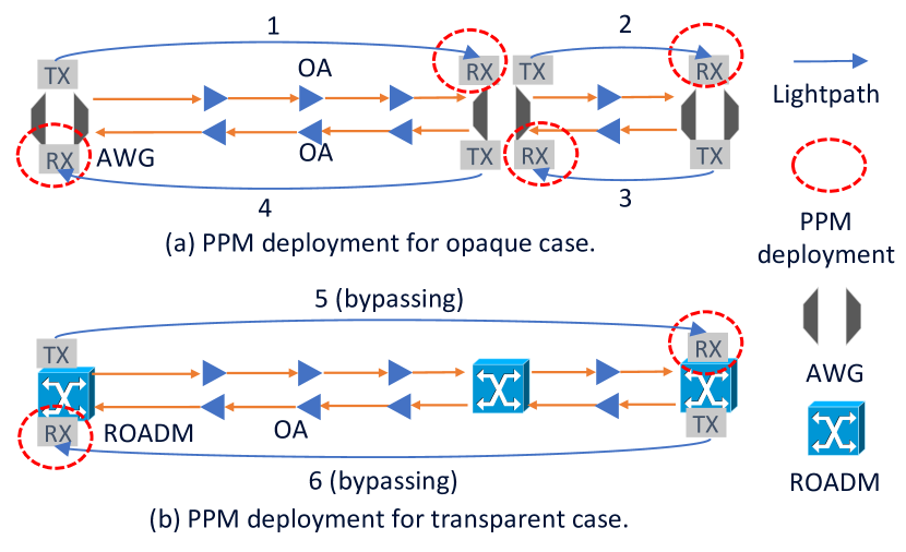
Figure 1: Network-wide PPM deployment.

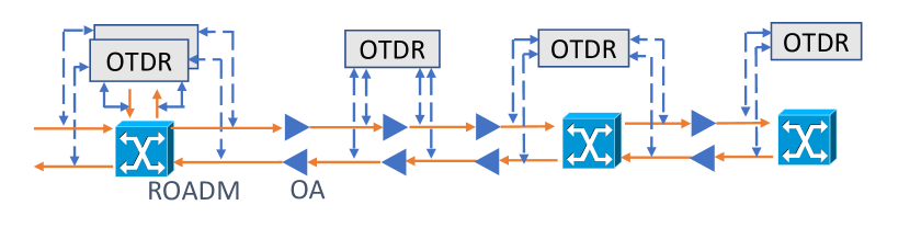
Figure 2: Network-wide OTDR deployment.

II-D Deployment of OTDR for Network Monitoring

A possible network-wide OTDR deployment for transparent network architecture is shown in Fig. 2, which can also be applied to opaque architecture. Let us assume the network is denoted by $G=(N,E)$, where $N$ is the set of physical nodes and $E$ is the set of physical links. The number of spans in link $(i,j)$ and the degrees of node $i$ are denoted with $s_{(i,j)}$ and $d_{i}$, respectively. One OTDR card serves 4 fiber links. We assume that no additional optical components except OTDR are used for monitoring, hence OTDRs are needed in every degree of nodes and every inline amplifier (one OTDR can cover both directions as in Fig. 2). Since we assume a bidirectional network with two fibers per degree, the number of OTDRs for node $i$ is $\lceil\frac{2d_{i}}{4}\rceil$. The number of inline amplifiers that need to be monitored in link $(i,j)$ is $max(0,\lceil\frac{s_{(i,j)}-2}{2}\rceil)$ as the two spans close to both end nodes are monitored with the OTDR for nodes. Hence, the number of OTDRs required in a network can be calculated using the equation below, which applies to both opaque and transparent architectures:

$$\small P=\sum\limits_{(i,j)\in E}max(0,\lceil\frac{s_{(i,j)}-2}{2}\rceil)+\sum\limits_{i\in N}\lceil\frac{2d_{i}}{4}\rceil$$ (1)

II-E Related Work on Monitoring Placement

The study of monitoring placement problems in optical networks dates back to the early 2000’s, but it has been revamped more recently following the growing importance of monitoring for network automation [23, 24, 25, 2]. Existing studies focus primarily on reducing the cost of monitors in two scenarios. In the first scenario, the objective is to minimize the number of monitors required to determine the faulty (or suspected faulty) network elements [23, 2, 26]. These works are based on machine learning algorithms [2] or heuristic algorithms [23, 26], and work under the assumption that, when an abnormal signal is detected on a monitor, at least one network element before the monitor in the corresponding LP is a faulty element. In the second scenario, the objective is again to minimize the number of placed monitors, but in this case, the constraint is to guarantee accurate assessment of some physical metrics (e.g., OSNR, power, etc.) for continuous network optimization (e.g., reduce the network margin) [24, 25]. For instance, Ref. [24] minimizes the number of monitors in the network to assess the quality of transmission (QoT) of all the established connections. Unlike previous optical network monitors , which obtain physical metrics at specific locations, PPM monitors power at each point along the optical line, reducing the number of necessary monitors in an optical line to just one. Thus, monitoring placement of PPM is different from previous works on optical network monitoring, and has not been investigated before. Although problems similar to PPM monitoring placement have also been solved in other communication networks (e.g., wireless sensor networks) [27] where one monitor monitors multiple devices/locations, our work still has several key distinctions. Specifically, unlike works for other communication networks [27], where the potential monitoring placement locations are fixed, our study investigated the monitoring placement of PPM when LPs (i.e., potential monitoring placement locations) vary with traffic loads. Furthermore, we do not only optimize the number of monitors as in Ref. [27], but also perform a sensitivity analysis to compare the cost and power consumption of PPM to that of OTDR, providing guidelines for future implementations.

III Optimized Monitoring Placement

In this section, we first formally define the OMP problem. To solve the problem, we formulate an ILP model and propose a scalable heuristic algorithm.

III-A Problem Statement

This study considers placing PPMs on an initial set of LPs obtained from an existing heuristic algorithm in Ref [16] that minimizes the number of transponders used to serve requests. The reach table of the considered transponder is shown in Table II, which is based on Ref. [28] and subject to slight modification during internal verification of Nokia. To evaluate improving the monitoring accuracy of PPM with several LPs, we defined a new metric called Number of PPMs per Link (NPL, defined as the number of monitored LPs that traverse the link). When the network is in low load, some links may not be monitored with the required NPL, as these links are not traversed by enough LPs.

TABLE II: Reach table for long-haul transponders.

Data rate (Gb/s)	Modulation format	Spacing (GHz)	Reach (km)
800	PCS 64 QAM	100	150
700	PCS 64 QAM	100	400
600	16 QAM	100	700
500	PCS 16 QAM	100	1300
400	PCS 16 QAM	100	2500
300	PCS 16 QAM	100	4700
200	PCS 16 QAM	100	5700

The problem of optimized monitoring placement (OMP) of PPM can be stated as follows: Given a network topology and a set of LPs, Decide the placement of PPM modules, Constrained by placing PPMs over the existing LPs, with the Objective of minimizing the unsatisfied NPL (defined as the additional number of monitors required to achieve the required NPL) in all links as the first objective and minimizing the number of PPM modules as the second objective.

III-B NP-hardness of the OMP Problem

We prove that the OMP problem is NP-hard when all the links can achieve the required NPL with Theorem 1 as follows.

Theorem 1: The OMP problem is NP-hard when all the links can achieve the required NPL (i.e., there are enough LPs such that all the links can be monitored with the required number of monitors, denoted with $\gamma$).

Proof: First, we show that a simplified version of OMP, where the number of LPs that exclusively traverse all edges in each physical path $l\in L$ is at most 1, is NP-hard. Since all links can achieve the required NPL, all links are monitored with $\gamma$ PPMs after satisfying the primary objective. Then, the simplified OMP problem (i.e., OMP problem of satisfying the second objective) can be stated as follows: Given a set of links and a set of LPs, Decide the placement of PPM modules, Constrained by satisfying the required NPL of all links, with the Objective of minimizing the number PPM modules. We show as follows that the set k-cover problem [29], a known NP-hard problem, can be reduced to the decision version of the simplified OMP problem.

The set k-cover problem can be stated as follows: Given a set $E$ of $|E|$ elements, a collection $S={S_{1},S_{2},...,S_{m}}$ of $m$ subsets of $E$, parameter $\delta_{l}^{e}$ of whether subset $S_{l}$ contains element $e$, an integer $\gamma$, and an integer $v$, does there exist a set of no more than $v$ subsets (defined as $I=\{S_{1},...,S_{v}\}\subseteq S$) such that $\sum\limits_{S_{l}\in I}\delta_{l}^{e}\geq\gamma$ for all $e\in E$. Given an instance of the set k-cover problem, an instance of the decision version of the simplified version of the OMP problem can be constructed as follows. Assume that the set of edges is denoted with $E$, and the set of traversed edges of physical path $l$ is denoted with $S_{l}$. The parameter $\delta_{l}^{e}$ corresponds to whether a physical path $l$ traverses edge $e$. The integer $\gamma$ denotes the required NPL. The corresponding question becomes whether a solution to the simplified OMP problem exists, such that the number of selected physical paths to monitor with PPMs is no more than $v$. The simplified OMP problem reaches the optimum if and only if the set k-cover problem reaches the optimum. In conclusion, the OMP problem is NP-hard when all links can achieve the required NPL.

III-C Integer Linear Programming Model for OMP Problem

The sets and parameters for the ILP model are shown in Table III, and the variables are shown in Table IV.

TABLE III: Sets and parameters for the ILP Model

Notation	Description
$E$	Set of physical links
$L$	Set of physical paths
$c_{l}$	Number of LPs that exclusively traverse all edges
	in physical path $l\in L$
$\delta_{l}^{e}$	Equals to 1 if physical path $l\in L$ traverses $e\in E$
$\gamma$	Required NPL
$\alpha$	Weight of number of unsatisfied of PPMs

TABLE IV: Variables for the ILP Model

Notation	Description
$p_{l}$	Integer, number of monitored LPs exclusively
	traversing all edges in physical path $l\in L$
$x_{e}$	Integer, number of PPMs for $e\in E$

The objective function of the ILP model is shown in Eqn. (2), where $\sum\nolimits_{e\in E}x_{e}$ denotes the sum of unsatisfied NPL in all links and $\sum\nolimits_{l\in L}p_{l}$ denotes the number of PPMs used. The weight $\alpha$ is set to be greater than the maximum number of hops of all physical paths in the network to prioritize minimizing unsatisfied NPL rather than reducing the PPM modules used.

The constraints of the ILP model are listed in Eqn. (3)-Eqn. (5). Eqn. (3) ensures the upper bound of the achieved NPLs for all links. Eqn. (4) ensures that the number of PPMs for link $e\in E$ is less or equal to the number of monitored LPs that traverse link $e$. Eqn. (5) ensures that the number of monitored LPs exclusively traversing all edges in physical path $l\in L$ should be smaller or equal to the number of available LPs.

$$\min\hskip 10.0pt\alpha\sum\limits_{e\in E}(\gamma-x_{e})+\sum\limits_{l\in L}p_{l}$$ (2)

$$x_{e}\leq\gamma\quad\forall e\in E$$ (3)

$$x_{e}\leq\sum\limits_{l\in L}\delta_{l}^{e}p_{l}\quad\forall e\in E$$ (4)

$$p_{l}\leq c_{l}\quad\forall l\in L$$ (5)

III-D Optimized Monitoring Placement Algorithm

We developed a new OMP algorithm to reduce the number of PPMs for monitoring. The OMP algorithm is designed leveraging existing effective heuristic algorithms for the set covering problem as in Ref. [30]. Note that this problem is different from the failure localization problem, as the OMP problem aims to deploy monitoring modules, while the failure localization problem [22, 31] aims to localize the soft/hard failure in the network based on the monitoring data.

Algorithm 1 Optimized monitoring placement algorithm.

1:Input: Network topology $G=(N,E)$, $L$, $c_{l}$, NPL $\gamma$, $d_{max}$

2:Output: Placement of PPM

3:Initialize $L_{m}\leftarrow L$, $E_{m}\leftarrow E$

4:Initialize covering matrix $M$ with $|E|$ rows and $|L|$ columns

5:for $e\in E$ do

6:    $x_{e}\leftarrow 0,z_{e}=\sum\limits_{l\in L}c_{l}M_{(e,l)}$

7:if architecture is opaque then

8:    for each $l\in L$ do

9:         $x_{e}\leftarrow min(c_{l},\gamma)$    

10:    Return

11:while $|E_{m}|>0$ do

12:    if All elements in $M$ is empty then

13:         Break     

14:    Obtain set $L_{s}$ such that $v_{l^{*}}\geq max\{v_{l}|l\in L_{m}\},\forall l^{*}\in L_{s}$

15:    $l_{s}\leftarrow-1,cost_{l_{s}}\leftarrow Inf$

16:    for $l\in L_{s}$ do

17:         Obtain $cost_{l}$ for LP $l$

18:         if $cost_{l}<cost_{l_{s}}$ then

19:             $l_{s}\leftarrow l,cost_{l_{s}}\leftarrow cost_{l}$              

20:    for $e$ in traversed edges of LP $l_{s}$ do

21:         $x_{e}\leftarrow x_{e}+1$, $z_{e}\leftarrow z_{e}-1$

22:         if $x_{e}\geq\gamma$ then

23:             Let $M_{(e,l_{s})}\leftarrow 0,\forall l_{s}\in L_{m}$

24:             Let $E_{m}\leftarrow E_{m}\setminus\{e\}$, $z_{e}\leftarrow 0$              

25:    if $p_{l_{s}}\geq c_{l_{s}}$ then

26:         Let $L_{m}\leftarrow L_{m}\setminus\{{l_{s}}\}$

27:         Let $M_{(e,l_{s})}\leftarrow 0,\forall e\in E$     

In the following, we illustrate the details of the proposed OMP algorithm through Algorithm. 1. The input $L$ denotes the set of physical paths, and the input $c_{l}$ denotes the number of LPs that traverse a path $l\in L$. The inputs $\gamma$ denote the required NPL.

The algorithm first initializes the sets and variables. Specifically, set $L_{m}$ denotes the set of physical paths that have unmonitored LPs exclusively traversing it, and set $E_{m}$ denotes the set of links that do not satisfy the required NPL. Then, the algorithm initializes the covering matrix $M$, where each column corresponds to a physical path and has $|E|$ elements (line 4). An element in the matrix $M$ equals one when the corresponding column represents a physical path containing the corresponding edge, and there are unmonitored LPs traversing this physical path. Assume that $z_{e}$ denotes the number of unmonitored LPs that traverse $e$ when $e$ does not satisfy the required NPL. Otherwise, $z_{e}$ equals to 0. After initializing $M$, the algorithm sets the initial value of the achieved NPL for each link (denoted as $x_{e}$) and $z_{e}$ (lines 5-6).

Then, the algorithm decides the PPM placement according to the network architecture (line 7-27). If the network architecture is opaque, all the LPs have only one hop, and the placement of PPM on LPs that exclusively traverse a physical path does not affect the placement of PPM on LPs that exclusively traverse any other physical path. Thus, the algorithm can simply loop over all path $l\in L$ and decide the number of PPMs placed on the LPs that exclusively traverse $l$ (line 7-10). Instead, for transparent architecture, since different physical paths may have overlapping links, the algorithm decides the placement of PPM until all the links are monitored as follows (line 11-27). If no LP can monitor more edges, the algorithm stops monitoring links (line 12-13). Assume that the number of links that can be monitored with LP exclusively traversing physical path $l$ is defined as $v_{l}$ as in Eqn. (6). The algorithm first greedily finds the set of paths that can be used to monitor the maximum number of links (line 14). Specifically, the algorithm first obtains the set $L_{s}$ where each path $l^{*}\in L_{s}$ has the maximum $v_{l}$ among all the paths that can be monitored. Then, the algorithm tries to break the ties of the paths in $L_{s}$ with the cost of monitoring the LP (15-19). The cost of monitoring an LP is defined as $cost_{l}$ and can be calculated with Eqn. (7) and Eqn. (8). Specifically, as in Ref. [30], our algorithm gives priority to monitoring the edges that are covered by less LPs. The number of unmonitored LPs that can be used to monitor an edge $e$ is defined as in Eqn. (7), and the cost of placing a PPM in an LP is defined to be positively correlated to the number of unmonitored LPs that can be used to monitor all edges in LP as in Eqn. (8). After selecting the LP that traverses path $l_{s}$ to monitor, the algorithm updates NPL for the link (i.e., $x_{e}$) and $z_{e}$ (line 21). If the NPL of a link achieves the required NPL, the corresponding row of the link in $M$ is set to 0, indicating that the link does not need more monitors (line 23). In addition, link $e$ is removed from the set of links that need to be monitored, and $z_{e}$ will be set to 0 (line 24). At last, if all the LPs that exclusively traverse path $l_{s}$ are monitored, path $l_{s}$ will be removed from the set of paths that can be placed with monitors (line 26), and the corresponding column of the path in $M$ is set to 0 (line 27).

$$v_{l}=\sum\limits_{e\in E_{l}}M_{(e,l)}\quad\forall l\in L$$ (6)

$$z_{e}=\sum\limits_{l\in L}(c_{l}-p_{l})M_{(e,l)}\quad\forall e\in E$$ (7)

$$cost_{l}=\frac{1}{\sum\limits_{e\in E_{l}}1/z_{e}}$$ (8)

The OMP algorithm is illustrated in Fig. 3, where we consider only one direction, for the sake of simplicity. Fig. 3(a) shows a simple physical network and seven candidate LPs. No LP is longer than two hops, e.g., due to the limited reach of transponders. Assume that the required NPL is 1. The covering matrix $M$ is shown in Fig. 3(b), representing whether additional edges can be monitored when selecting a path. The algorithm iteratively selects new LPs to monitor until all the links are monitored. At each iteration, the algorithm requires two stages. In stage 1, the algorithm identifies the LPs that allow to cover (monitor) the maximum number of edges, i.e., it selects the columns with the maximum $v_{l}$ as defined in Eqn. (6) (listed in the last row of the table in Fig. 3(b)). In stage 2, the algorithm selects, among the columns identified in stage 1, the column (i.e., the physical path) that has a minimum value of $cost_{l}$ as in Eqn. (8). In case of ties, OMP randomly selects a column. In Fig. 3(b), after selecting LPs 1, 2, and 3 in phase 1, stage 2 calculates the cost of selecting LPs. Specifically, LP 1 and LP 3 have the smallest cost of 6/5 by calculating the cost with all the traversed edges (marked with red rows for LP 1 in Fig. 3)(b) using Eqn. (8). In the current iteration, the algorithm selects LP1. In the next iteration, the algorithm will select LP 3, and all the edges will be monitored. In summary, OMP reduces the PPM modules from 7 (one for each LP) to 2.

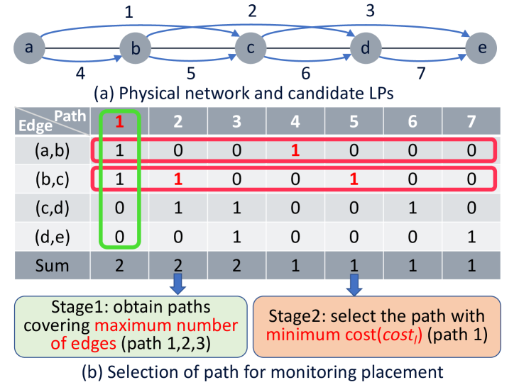
Figure 3: Illustration of the OMP algorithm.

Complexity of the algorithm: For opaque architecture, the algorithm iterates all physical paths (at most $|L|$) and decides the number of PPMs with the $min(c_{l},\gamma)$ operation, the complexity is $O(|L|)$. Instead, for transparent architectures, the complexity of the algorithm is mainly determined by the process of selecting the LPs to monitor (line 11-27). The number of iterations of selecting the LPs is at most $O(\gamma|E|$). Assume that the maximum number of hops of LPs is $H$. The complexity of selecting the set $L_{s}$ is $O(H|L|)$. The complexity of calculating $cost_{l}$ is $H$, and hence the complexity of breaking ties of the paths in $L_{s}$ is $O(H|L_{s}|)$. The complexity of updating the matrix $M$ after selecting the LP to monitor is $O(H|L|)$. Hence, the overall complexity is $O(\gamma|E|H|L|)$.

IV Illustrative Numerical Results

IV-A Simulation Settings

We implemented both the ILP formulation and the OMP algorithm using Python. The ILP formulation was solved with a state-of-the-art non-commercial solver, namely Solving Constraint Integer Programs (SCIP) solver [32]. The simulations are performed on a workstation with Intel(R) Core(TM) i5-13400F CPU processor and 32 GB of memory.

We first compare the ILP and the OMP algorithm in terms of the unsatisfied NPL and execution time over Gabriel graph topologies [33] with nodes ranging from 100 to 300 (Gabriel graphs have been shown to accurately characteristics of optical networks [34]). Then, we perform our numerical evaluations on both a national-scale and a continental-scale real network topology, the 14-node Japan (J14) [35] and the 14-node NSF (N14), respectively [36]. Specifically, we first evaluate the number of monitors under different loads, and then compare the cost and power consumption of PPM and OTDR. Note that, since ILP is scalable on both J14 and N14, all the evaluations on J14 and N14 are based on the optimal solutions of ILP. In addition, each fiber operates on a 6-THz C-band.

We consider PPM deployment in two network architectures, i.e., opaque (the cases with and without OMP are named as Op-O and Op, respectively) and transparent (the cases with and without OMP are named as Tr-O, Tr, respectively) architectures, which are compared to the OTDR deployment. When evaluating the number of monitors under different loads, some links are not crossed by any LP when network traffic is exceptionally low (less than 30 Tb/s). In this case, we do not deploy OTDR on links not traversed by any LPs. Since the LPs may vary between opaque and transparent architectures, the links not traversed by any LPs could also differ, potentially leading to a variation in the number of OTDRs deployed in different architectures. Note that the difference in the number of OTDRs for opaque and transparent architectures is less than 3% for all the tested cases only under very low traffic. Moreover, when comparing the cost and power consumption under 1% rejection rate, all the links are traversed by at least one LP due to higher traffic, leading to the same number of OTDRs deployed for both opaque and transparent architectures. Thus, we only show the results of OTDR with transparent network architectures for simplicity. When considering multiple NPLs, the cases with OMP and links with $\gamma$ monitors are named as Op-O-$\gamma$ and Tr-O-$\gamma$, for opaque and transparent architectures, respectively. Note that, without OMP, since we place one PPM in each receiver, the number of placed PPMs is a constant value regardless of the required NPL, and hence we do not need to add suffix -k for the cases without OMP (i.e., Op and Tr). For comparison between ILP and the OMP algorithm, we assume the transmission distance of long-haul transponders can be up to six hops in the network. Instead, for cost and power consumption analysis with N14 and J14, we use the distance in the real network. The requested data rate is randomly generated from 100Gb/s to 400Gb/s among all node pairs. We first increase the number of requests and evaluate the number of monitors under different loads. Then, we increase the number of requests until 1% of requests are blocked in transparent architecture, and we use the corresponding carried traffic to evaluate the cost and power consumption for both opaque and transparent architectures (note that opaque architecture can carry more traffic than transparent architecture). The normalized cost (energy) of a transponder and an OTDR module is 4 (8) and 0.2 (0.25), respectively. All the reported results are averaged over 10 instances.

IV-B Comparison of ILP and Heuristic Algorithm

In this section, we first compare the number of monitors and the execution time using ILP and the heuristic algorithm. The suffix OMP and ILP denote the method to solve the scenario. Fig. 4(a) shows the number of monitors under different numbers of network nodes. First, in the transparent architecture, the number of monitors is reduced up to 74% with respect to the opaque architecture, since LPs in transparent architecture have a larger number of hops due to bypassing. Regarding the gap between the OMP algorithm and the ILP, for opaque architecture, the optimality gap is 0% for all the tested cases. Instead, for transparent architecture, the optimality gap can be up to around 14.9%, because different LPs may partially overlap, and it is much more difficult to place PPMs for transparent architecture compared to that for opaque architecture. The performance of the OMP algorithm is achieved with a significant reduction of execution time, e.g., the execution time of transparent architecture reduces from about 4345 seconds to 1 second, as shown in Fig. 4(b).

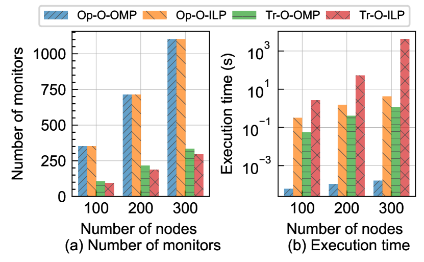
Figure 4: Comparison of the OMP algorithm and ILP.

IV-C Evaluation of Number of Monitors under Different Loads

In the following, we first evaluate the average unsatisfied NPL when increasing the traffic, and then we compare the number of monitors used.

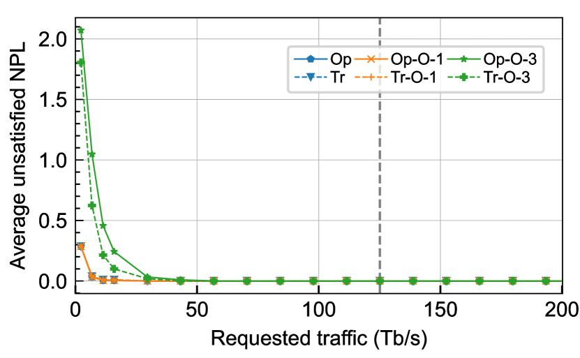
Figure 5: Average unsatisfied NPL vs. load in N14.

The unsatisfied NPL is reported in Fig. 5 where the solid dotted line represents the requested traffic under 1% rejection rate. When the requested traffic is less than 43Tb/s, the average unsatisfied NPL reduces when the requested traffic increases. This is because, with higher traffic, more LPs can be established, which can be placed with PPMs for monitoring. Note that for Op and Tr, since we do not optimize the achieved NPL, we consider that a link satisfies the required NPL if it is monitored by one PPM. Specifically, for Op and Tr, the unsatisfied NPL of a link equals 0 if the link has at least one monitor. Otherwise, the unsatisfied NPL of a link equals 1. Thus, the unsatisfied NPL of Op is the same as Op-O-1, and the unsatisfied NPL of Tr is the same as Tr-O-1. In addition, the lines representing Op-O-1 and Tr-O-1 almost overlap because the maximum difference between the unsatisfied NPL of Op-O-1 and Tr-O-1 is less than 0.005, indicating the number of links that are monitored with at least one PPM for opaque and transparent architectures are almost the same. Instead, with a low load, Tr-O-3 reduces up to around 100% of unsatisfied NPL of Op-O-3 because transparent architectures have a larger number of LPs due to smaller grooming capabilities. When the requested traffic is larger than 43Tb/s, the average unsatisfied NPL is 0 for all cases, indicating that the required NPL of all links in the network is satisfied.

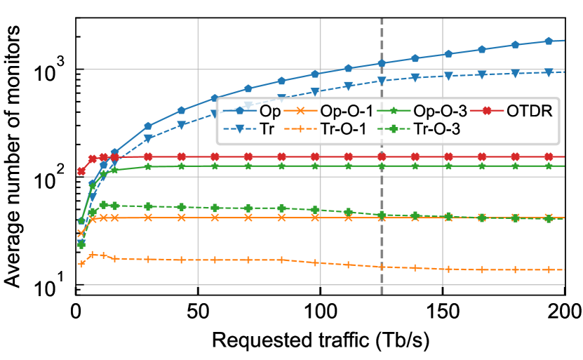
Figure 6: Average number of monitors vs. load in N14.

Let us now evaluate the number of monitors under different loads in N14 as in Fig. 6. The number of PPMs for Op and Tr always increases with the growing traffic due to the higher number of established LPs, and all LPs are equipped with PPMs. Note that OTDR modules are only placed to monitor the links that are monitored with PPM to have a fair comparison of OTDR and PPM. Therefore, as the traffic approaches 30Tb/s, the number of OTDRs increases to 154 and then remains constant, given that all links are already monitored by at least one PPM. With OMP, for Tr-O-1, the number of monitors increases up to 19 when the traffic grows to 7Tb/s because more links are monitored. Then, the number of monitors decreases from 19 to 15 when the traffic grows because more LPs with a larger number of hops can be used. Instead, for Op-O-1, the number of monitors never decreases since all LPs have only one hop. When NPL equals 3, the number of monitors of Op-O-3 and Tr-O-3 follows the consistent trend as in Op-O-1 and Tr-O-1. After all the links satisfy the required NPL, the number of required OTDRs is greater than all the tested cases that place PPM with OMP. For instance, the number of OTDRs required is around 7x to 11x the number of PPMs in Tr-O-1 when increasing the network traffic.

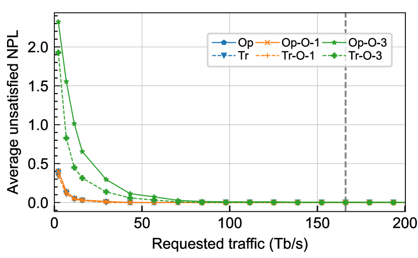
Figure 7: Average unsatisfied NPL vs. load in J14.

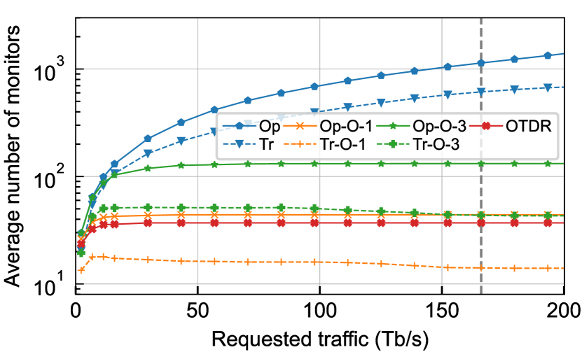
Figure 8: Average number of monitors vs. load in J14.

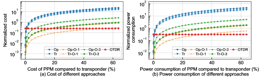
Figure 9: Cost of and power consumption of different approaches in N14.

The unsatisfied NPL in J14 is shown in Fig. 7. All the different approaches perform similarly to the unsatisfied NPL as in N14. Different from the results in N14, now there are no more unsatisfied NPL for all approaches when traffic reaches 99Tb/s (instead of 43Tb/s), because in J14, LPs can operate on higher modulation formats due to shorter link length, and hence fewer LPs are established to serve the same amount of traffic. Regarding the number of monitors, as shown in Fig. 8, all the approaches with PPM remain consistent trends as that in N14. The difference is that, in J14, the number of OTDRs required to monitor the whole network reduces from 154 in N14 to 37 in J14, since J14 has a much shorter link length. Consequently, the number of OTDR required is smaller than all the cases with PPM except Tr-O-1, as shown in Fig. 8.

TABLE V: Number of monitoring components

Scenarios	Op	Tr	Op-O-1	Tr-O-1	Op-O-3	Tr-O-3	OTDR
J14	1167	624	44	14	132	43	37
N14	1135	782	42	15	126	44	154

The analysis of the trends in the number of monitors indicates that, with optimized monitoring placement, the number of PPMs required has only a small variation with requested traffic unless under low-load traffic (e.g., less than 50 Tb/s, which corresponds to less than 30% of spectrum occupation for transparent architecture). Hence, in the following analysis, we compare the number of monitors under fixed traffic (i.e., traffic with 1% rejection probability for transparent architecture, which corresponds to around 60% and 70% of spectrum occupation of J14 and N14, respectively). Note that, for the traffic with 1% rejection probability, all the links can satisfy the required NPL for the tested cases. The number of monitoring components (i.e., either PPM or OTDR modules) used in J14 and N14 topologies are reported in Table V. First, without OMP, the number of PPM modules for Op is about 30x the number of OTDR in J14, while this value is reduced to 7.4x in N14, as OTDR now experiences an about 300% increase in N14 compared to J14 due to the fact that N14 has a much larger geographical dimension and hence much larger number of spans. With OMP, the number of PPM modules for Op-O is reduced to the number of edges in the network, as each edge is monitored with only one PPM module. Note that, in N14, for Op-O-1, the number of PPM modules even decreased to only 27% of OTDRs. Moreover, Tr-O-1 can further reduce up to 65% PPM modules by bypassing nodes. Specifically, the number of OTDR is about 10x the number of PPM, suggesting that the cost (power) of one PPM should be 10x lower than that of OTDR to be a competing technology. For J14, the number of OTDR is 2.6x the number of PPM due to the shorter link length, suggesting that the cost (power) of one PPM should be 2.6x lower than that of OTDR. When the required NPL is 3, the number of required monitors is around 3 times that of cases when the required NPL is equal to 1.

IV-D Evaluation of Cost and Power Consumption

We now evaluate the cost and power consumption of PPM compared to OTDR in N14 and J14.

Normalized cost in N14. Fig. 9(a) illustrates the normalized cost of monitoring per Tb/s for N14. We define the x-axis value of the point where PPM’s cost/power consumption is equal to OTDR as crossing value, which is also reported in Table VI. The cases with OMP have much smaller crossing values than the cases without OMP, showing that OMP is fundamental to lower PPM monitoring costs. Without OMP, the cost of one PPM must be less than 0.7% and 1.0% of one transponder for Op and Tr, respectively, to compete with OTDR. However, with OMP, the cost of PPM should be below 18.3% and 52.7% of the cost of transponder for Op-O-1 and Tr-O-1, respectively, to compete with OTDR. Note that the cost difference between Op-O-1 and Tr-O-1 is due to the bypassing of nodes in the transparent architecture. Moreover, when the required NPL is 3, the crossing value of cost is reduced to around 1/3 of that of the cases with the required NPL equal to 1. Specifically, the crossing value of Op-O-3 and Tr-O-3 is 6.1% and 17.4%, respectively.

TABLE VI: Crossing values of PPM with OTDR in N14

Scenarios	Op	Tr	Op-O-1	Tr-O-1	Op-O-3	Tr-O-3
Cost	0.7	1.0	18.3	52.7	6.1	17.4
Power consumption	0.4	0.6	11.5	33.0	3.8	10.9

Normalized power consumption in N14. Fig. 9(b) plots the power consumption of PPM compared to OTDR. Without OMP, the power consumption of PPM relative to one transponder must be less than 0.4% and 0.6% of the transponder’s power consumption. With OMP, the power consumption of PPM can be up to 11.5% and 33.0% of the transponder’s power consumption for Op-O-1 and Tr-O-1, respectively. When the required NPL is 3, the crossing value of power consumption is reduced to around 1/3 that of the cases when the required NPL is 1.

Normalized cost and power consumption in J14. The overall trends of cost and power consumption in J14 are similar to N14. Table VII reports the crossing values for J14. Different from N14, PPM can perform better than OTDR only with a much lower cost and power consumption than one transponder. This is because less OTDRs are deployed in links in a smaller topology. Specifically, PPM’s cost and power consumption are reduced to approximately 0.2% and 0.1% for Op, and 0.3% and 0.2% for Tr, respectively. Moreover, with OMP, the crossing values of cost and power consumption are also significantly reduced. For instance, the crossing values of cost and power consumption for Tr-O-1 are reduced from 52.7% to 13.2% and 33.0% to 8.3% for transparent architecture.

TABLE VII: Crossing values of PPM with OTDR in J14

Scenarios	Op	Tr	Op-O-1	Tr-O-1	Op-O-3	Tr-O-3
Cost	0.2	0.3	4.2	13.2	1.4	4.3
Power consumption	0.1	0.2	2.6	8.3	0.9	2.7

V Conclusion

Following the recent experimentation of PPM as a novel monitoring solution, in this work, we investigated the problem of optimized monitoring placement for PPM, and we quantified the cost and power consumption of PPM compared to OTDR to provide guidelines for deployment of PPM modules. Results show that, for a nation-wide topology as J14, cost (power consumption) of the PPM should be below 2.6 times that of OTDR, which corresponds to 13% (8%) of that of a transponder. Instead, in a larger continental-wide topology as N14, PPM’s cost (power consumption) should be below 10.2 times that of OTDR, which corresponds to 53% (33%) of that of a transponder. This means that the cost and power consumption of PPM are not limiting factors for PPM deployments, as PPM is not expected to have such a high cost and power consumption. In the future, we plan to deploy PPMs in the field to evaluate their cost and power consumption further.

References

- [1] Y. He, Z. Zhai, L. Dou, L. Wang, Y. Yan, C. Xie, C. Lu, and A. P. T. Lau, “Improved qot estimations through refined signal power measurements and data-driven parameter optimizations in a disaggregated and partially loaded live production network,” IEEE/OSA Journal of Optical Communications and Networking, vol. 15, no. 9, pp. 638–648, 2023.
- [2] R. Wang, J. Zhang, S. Yan, C. Zeng, H. Yu, Z. Gu, B. Zhang, T. Taleb, and Y. Ji, “Suspect fault screen assisted graph aggregation network for intra-/inter-node failure localization in roadm-based optical networks,” IEEE/OSA Journal of Optical Communications and Networking, vol. 15, no. 7, pp. C88–C99, 2023.
- [3] Y. R. Zhou, K. Smith, P. Weir, A. Lord, J. Chen, W. Pan, N. Zhou, and Z. Xiao, “Field trial demonstration of novel optical superchannel capacity protection for 400g using dp–16qam and dp–qpsk with in-service otdr fault localization,” in Optical Fiber Communication Conference (OFC), 2016.
- [4] D. R. Anderson, L. M. Johnson, and F. G. Bell, Troubleshooting optical fiber networks: understanding and using optical time-domain reflectometers. Elsevier, 2004.
- [5] B. Jander, L. Garrett, R. Kram, L. Richardson, Y. Xu, M. Rodriguez, D. Pappas, Y. Jiang, Y. Chai, T. Verdi, J. Giotis, and F. Ayadi, “Enhanced undersea line monitoring technology for coherent open cable systems,” in SubOptic Conference, 2019.
- [6] C. Hahn, J. Chang, and Z. Jiang, “Monitoring of generalized optical signal-to-noise ratio using in-band spectral correlation method,” in European Conference on Optical Communication (ECOC), 2022.
- [7] T. Sasai, Y. Sone, E. Yamazaki, M. Nakamura, and Y. Kisaka, “A generalized method for fiber-longitudinal power profile estimation,” in European Conference on Optical Communication (ECOC), 2023.
- [8] A. May, F. Boitier, A. C. Meseguer, J. U. Esparza, P. Plantady, A. Calsat, and P. Layec, “Longitudinal power monitoring over a deployed 10,000-km link for submarine systems,” in Optical Fiber Communication Conference (OFC), 2023.
- [9] T. Tanimura, S. Yoshida, K. Tajima, S. Oda, and T. Hoshida, “Fiber-longitudinal anomaly position identification over multi-span transmission link out of receiver-end signals,” IEEE/OSA Journal of Lightwave Technology, vol. 38, no. 9, pp. 2726–2733, 2020.
- [10] A. May, F. Boitier, E. Awwad, P. Ramantanis, M. Lonardi, and P. Ciblat, “Receiver-based experimental estimation of power losses in optical networks,” IEEE Photonics Technology Letters, vol. 33, no. 22, pp. 1238–1241, 2021.
- [11] I. Kim, O. Vassilieva, R. Shinzaki, M. Eto, S. Oda, and P. Palacharla, “Multi-channel longitudinal power profile estimation,” in European Conference on Optical Communication (ECOC), 2023.
- [12] Cisco. Cisco Network Convergence System 1001 OTDR Line Card Data Sheet. https://www.cisco.com/c/en/us/products/collateral/optical-networking/network-convergence-system-1000-series/datasheet-c78-742294.html/, accessed on 18/02/2024.
- [13] T. Sasai, M. Takahashi, M. Nakamura, E. Yamazaki, and Y. Kisaka, “Linear least squares estimation of fiber-longitudinal optical power profile,” Journal of Lightwave Technology, vol. 42, no. 6, pp. 1955–1965, 2024.
- [14] Kingfisherfiber. Specifications for OTDR Handheld Optical Time Domain Reflectometer. https://kingfisherfiber.com/media/2246/6700-otdr.pdf, accessed on 18/02/2024.
- [15] A. May, F. Boitier, A. Courilleau, B. Al Ayoubi, and P. Layec, “Demonstration of enhanced power losses characterization in optical networks,” in Optical Fiber Communication Conference (OFC), 2022, pp. Th1C–6.
- [16] Q. Zhang, A. Morea, and M. Tornatore, “A pragmatic power-consumption analysis for ipowdm networks with zr/zr modules,” in European Conference on Optical Communication (ECOC), 2022.
- [17] Q. Zhang, P. Layec, A. Morea, and M. Tornatore, “Cost and power-consumption analysis for power profile monitoring in optical networks,” in European Conference on Optical Communication (ECOC), 2023.
- [18] T. Sasai, M. Nakamura, E. Yamazaki, S. Yamamoto, H. Nishizawa, and Y. Kisaka, “Digital longitudinal monitoring of optical fiber communication link,” IEEE/OSA Journal of Lightwave Technology, vol. 40, no. 8, pp. 2390–2408, 2022.
- [19] T. Sasai, E. Yamazaki, and Y. Kisaka, “Performance limit of fiber-longitudinal power profile estimation methods,” IEEE/OSA Journal of Lightwave Technology, vol. 41, no. 11, pp. 3278–3289, 2023.
- [20] L. Andrenacci, G. Bosco, and D. Pilori, “Pdl localization and estimation through linear least squares-based longitudinal power monitoring,” IEEE Photonics Technology Letters, vol. 35, no. 24, pp. 1431–1434, 2023.
- [21] C. Hahn, J. Chang, and Z. Jiang, “Localization of reflection induced multi-path-interference over multi-span transmission link by receiver-side digital signal processing,” in Optical Fiber Communication Conference, 2022.
- [22] C. Delezoide, P. Ramantanis, L. Gifre, F. Boitier, and P. Layec, “Field trial of failure localization in a backbone optical network,” in European Conference on Optical Communication (ECOC), 2021.
- [23] C. M. Machuca and I. Tomkos, “Optimal monitoring equipment placement for fault and attack location in transparent optical networks,” in International Conference on Research in Networking. Springer, 2004, pp. 1395–1400.
- [24] M. Angelou, Y. Pointurier, D. Careglio, S. Spadaro, and I. Tomkos, “Optimized monitor placement for accurate qot assessment in core optical networks,” IEEE/OSA Journal of Optical Communications and Networking, vol. 4, no. 1, pp. 15–24, 2012.
- [25] P. K. Thiruvasagam, A. Chakraborty, A. Mathew, and C. S. R. Murthy, “Reliable placement of service function chains and virtual monitoring functions with minimal cost in softwarized 5g networks,” IEEE Transactions on Network and Service Management, vol. 18, no. 2, pp. 1491–1507, 2021.
- [26] C. M. Machuca and M. Kiese, “Optimal placement of monitoring equipment in transparent optical networks,” in 2007 6th International Workshop on Design and Reliable Communication Networks. IEEE, 2007, pp. 1–6.
- [27] Z. Abrams, A. Goel, and S. Plotkin, “Set k-cover algorithms for energy efficient monitoring in wireless sensor networks,” in Proceedings of the 3rd international symposium on Information processing in sensor networks, 2004, pp. 424–432.
- [28] T. Zami, B. Lavigne, and M. Lefrançois, “Added value of 90 gbaud transponders for wdm networks,” in Optical Fiber Communications Conference and Exhibition (OFC), 2020.
- [29] S. Slijepcevic and M. Potkonjak, “Power efficient organization of wireless sensor networks,” in IEEE International Conference on Communications (ICC), 2001.
- [30] F. J. Vasko, Y. Lu, and K. Zyma, “What is the best greedy-like heuristic for the weighted set covering problem?” Operations Research Letters, vol. 44, no. 3, pp. 366–369, 2016.
- [31] K. Christodoulopoulos, N. Sambo, and E. Varvarigos, “Exploiting network kriging for fault localization,” in Optical fiber communication conference (OFC), 2016.
- [32] K. Bestuzheva, M. Besançon, W.-K. Chen, A. Chmiela, T. Donkiewicz, J. van Doornmalen, L. Eifler, O. Gaul, G. Gamrath, A. Gleixner et al., “Enabling research through the scip optimization suite 8.0,” ACM Transactions on Mathematical Software, vol. 49, no. 2, pp. 1–21, 2023.
- [33] K. R. Gabriel and R. R. Sokal, “A new statistical approach to geographic variation analysis,” Systematic zoology, vol. 18, no. 3, pp. 259–278, 1969.
- [34] J. Velinska, M. Mirchev, and I. Mishkovski, “Optical networks’ topologies: costs, routing and wavelength assignment,” Optical Networks, p. 10, 2017.
- [35] M. Ibrahimi, H. Abdollahi, C. Rottondi, A. Giusti, A. Ferrari, V. Curri, and M. Tornatore, “Machine learning regression for qot estimation of unestablished lightpaths,” IEEE/OSA Journal of Optical Communications and Networking, vol. 13, no. 4, pp. B92–B101, 2021.
- [36] B. G. Bathula and J. M. Elmirghani, “Constraint-based anycasting over optical burst switched networks,” IEEE/OSA Journal of Optical Communications and Networking, vol. 1, no. 2, pp. A35–A43, 2009.