Entropy-Informed Weighting Channel Normalizing Flow

Abstract

Normalizing Flows (NFs) have gained popularity among deep generative models due to their ability to provide exact likelihood estimation and efficient sampling. However, a crucial limitation of NFs is their substantial memory requirements, arising from maintaining the dimension of the latent space equal to that of the input space. Multi-scale architectures bypass this limitation by progressively reducing the dimension of latent variables while ensuring reversibility. Existing multi-scale architectures split the latent variables in a simple, static manner at the channel level, compromising NFs’ expressive power. To address this issue, we propose a regularized and feature-dependent $\mathtt{Shuffle}$ operation and integrate it into vanilla multi-scale architecture. This operation heuristically generates channel-wise weights and adaptively shuffles latent variables before splitting them with these weights. We observe that such operation guides the variables to evolve in the direction of entropy increase, hence we refer to NFs with the $\mathtt{Shuffle}$ operation as Entropy-Informed Weighting Channel Normalizing Flow (EIW-Flow). Experimental results indicate that the EIW-Flow achieves state-of-the-art density estimation results and comparable sample quality on CIFAR-10, CelebA and ImageNet datasets, with negligible additional computational overhead.

Keywords Normalizing Flows $\cdot$ Multi-Scale Architecture $\cdot$ Shuffle Operation $\cdot$ EIW-Flow $\cdot$ Entropy

1 Introduction

Deep generative models are a type of machine learning paradigm that revolves around learning the probability distribution of data. These models are designed to generate new samples based on the learned data distribution, especially when there is a lack of data available for training. Although it can be challenging to learn the true distribution of data due to practical factors, deep generative models have been proven to approximate it effectively[62]. This has made them very useful in a variety of downstream pattern recognition tasks, such as image synthesis[52], image re-scaling[91], 3D point cloud upsampling[90], and abstract automatic speaker verification[81]. In recent years, deep generative models have gained widespread attention and research[6, 77, 94], which has led to significant advances in the field.

Popular deep generative models like Generative Adversarial Networks (GANs) [5] model the underlying true data distribution implicitly, but do not employ the maximum likelihood criterion for analysis. Variational autoencoders (VAEs) [52] map data into a low-dimensional latent space for efficient training, resulting in optimizing a lower bound of the log-likelihood of data. Different from GANs and VAEs, Autoregressive Flows [60] and Normalizing Flows are both inference models that directly learn the log-likelihood of data. Although Autoregressive Flows excel at capturing complex and long-term dependencies within data dimensions, their sequential synthesis process makes parallel processing difficult, leading to limited sampling speed.

Normalizing Flows (NFs) define a series of reversible transformations between the true data distribution and a known base distribution (e.g., a standard normal distribution). These transformations are elucidated in works like NICE [2], Real NVP [3] and GLOW [6]. NFs have the advantage of exact estimation for the likelihood of data. Additionally, the sampling process of NFs is considerably easier to parallelize than Autoregressive Flows and can be optimized directly compared to GANs. However, a significant challenge for NFs lies in efficiently achieving a high level of expressive power in the high-dimensional latent space. This challenge arises because data typically lies in a high-dimensional manifold, and it is essential for NFs to maintain the dimension across the inference or sampling process to ensure its reversibility.

In order to mitigate this problem, Real NVP introduced a multi-scale architecture that progressively reduces the dimension of latent variables while ensuring its reversibility. This architecture aids in accelerating training and save memory resources [65]. However, the $\mathtt{Split}$ operation employed in the multi-scale architecture compromises NFs’ expressive power as it simply splits the high-dimensional variable into two lower-dimensional variables of equal size. As a result, it does not take into account the interdependencies between different channel feature maps of the variable, which can restrict the NFs’ overall expressive power.

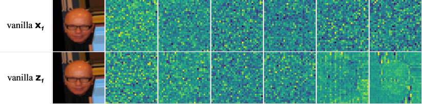
Figure 1: Some channel feature maps before the $\mathtt{Split}$ operation in multi-scale architecture, without applying our proposed $\mathtt{Shuffle}$ operation. The first column shows facial images from the CelebA dataset, while the remaining columns display the corresponding channel feature maps of these faces. Specifically, the top row and the bottom row depict channel feature maps of $\mathbf{x}_{1}$ and $\mathbf{z}_{1}$, respectively, which are the outputs of the first scale of NFs.

As illustrated in Fig. 1, it can be observed that some channel feature maps of $\mathbf{z}_{1}$ contain facial contour information. However, $\mathbf{z}_{1}$ is assumed to follow a Gaussian distribution within the framework of NFs, implying that traditional NFs with multi-scale architecture cannot capture such salient information, consequently compromising their efficacy and expressive power.

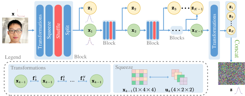
Figure 2: Schematic diagram of improved inference process with multi-scale architecture. Compared to vanilla architecture, an additional $\mathtt{Shuffle}$ operation is introduced to adaptively shuffle and propagate relatively information-rich channel feature maps to the next scale. For some latent variable, there are red and blue dashed lines, where the former denotes the true distribution of the variable, and the latter represents the standard Gaussian distribution.

To enhance the efficacy and expressive power of NFs with multi-scale architecture, we propose a regularized $\mathtt{Shuffle}$ operation applied before the $\mathtt{Split}$ operation in the inference process. This operation involves assigning weights to each channel feature map based on the feature information it contains. The input data is then shuffled across channel dimensions according to these weights, while still maintaining the reversibility of NFs. More importantly, we demonstrate that channel feature maps with higher entropy, which are more likely to follow a Gaussian distribution, will be used to form the final latent variable through our proposed $\mathtt{Shuffle}$ operation. Based on this operation, we improve the conventional multi-scale architecture and propose a novel normalizing flow model called “Entropy-Informed Weighting Channel Normalizing Flow" (EIW-Flow). The schematic diagram of our improved multi-scale architecture is shown in Fig. 2.

The main contributions in this paper are as follows:

1. We design a regularized $\mathtt{Shuffle}$ operation to adaptively shuffle the channel feature maps of its input based on the feature information contained in each map, while maintaining the reversibility of NFs.

2. We propose to divide the $\mathtt{Shuffle}$ operation into three distinct components: the solver-$\mathcal{S}$, the guider-$\mathcal{G}$ and the shuffler-$\mathcal{S}_{\mathcal{F}}$ (see 3.1 for details).

3. We demonstrate the efficacy of the $\mathtt{Shuffle}$ operation from the perspective of entropy using the principles of information theory and statistics, such as the Central Limit Theorem and the Maximum Entropy Principle.

4. Our experiments show state-of-the-art results on density estimation and comparable sampling quality with a negligible additional computational overhead.

2 Background

In this section, we review the basics of deep generative models and Normalizing Flows. We then discuss the multi-scale architecture and its bottleneck problem.

2.1 Deep Generative Models

Let $\mathbf{x}$ be a random variable with complex unknown distribution $p(\mathbf{x})$ and i.i.d. dataset $\mathcal{X}$. The main goal of generative models is to define a parametric distribution $q_{\boldsymbol{\theta}}(\mathbf{x})$ and learn its optimal parameters $\boldsymbol{\theta}^{*}$ to approximate the true but unknown data distribution $p(\mathbf{x})$ [84].

An efficient and tractable criterion is Maximum Likelihood (ML):

$$\boldsymbol{\theta}^{*}=\mathop{\arg\max}\limits_{\boldsymbol{\theta}\in\boldsymbol{\Theta}}\mathbb{E}_{\mathbf{x}\sim p(\mathbf{x})}[\log q_{\boldsymbol{\theta}}(\mathbf{x})].$$ (1)

In this case, the optimal parameters $\boldsymbol{\theta}^{*}$ can be learned iteratively using optimizers based on gradient descent methods such as SGD [1].

2.2 Normalizing Flows

Normalizing Flows (NFs) define an isomorphism $\mathbf{f}$ with parameters $\boldsymbol{\theta}$ that transform the observed data $\mathbf{x}$ in $\mathcal{X}$ to a corresponding latent variable $\mathbf{z}$ in a latent space $\mathcal{Z}$,

$$\mathbf{z}=\mathbf{f}(\mathbf{x})\quad\text{and}\quad\mathbf{x}=\mathbf{f}^{-1}(\mathbf{z}).$$ (2)

In practice, $\mathbf{f}$ is usually composed of a series of isomorphisms $\{\mathbf{f}_{k}\}_{k=1}^{K}$, i.e. $\mathbf{f}=\mathbf{f}_{K}\circ\mathbf{f}_{K-1}\circ\cdots\circ\mathbf{f}_{1}$. And each $\mathbf{f}_{k}$ transforms intermediate variable $\mathbf{x}_{k-1}$ to $\mathbf{x}_{k}$, where $\mathbf{x}_{0}\triangleq\mathbf{x}$ and $\mathbf{x}_{K}\triangleq\mathbf{z}$. Consequently, NFs can be summarized as:

$$\mathbf{z}\stackrel{{\scriptstyle\mathbf{f}_{K}}}{{\longleftrightarrow}}\cdots\stackrel{{\scriptstyle\mathbf{f}_{3}}}{{\longleftrightarrow}}\mathbf{x}_{2}\stackrel{{\scriptstyle\mathbf{f}_{2}}}{{\longleftrightarrow}}\mathbf{x}_{1}\stackrel{{\scriptstyle\mathbf{f}_{1}}}{{\longleftrightarrow}}\mathbf{x},$$ (3)

where $\mathbf{z}$ follows a tractable and simple distribution such as isotropic Gaussian distribution $N(\boldsymbol{\mu},\sigma^{2}\mathbf{I})$.

Given that we can compute the log-likelihood $q_{\mathbf{z}}(\mathbf{z})$ of $\mathbf{z}$, the unknown likelihood $q_{\boldsymbol{\theta}}(\mathbf{x})$ of $\mathbf{x}$ under the transformations $\{\mathbf{f}_{k}\}_{k=1}^{K}$ can be computed by using the change of variables formula,

$$\log q_{\mathbf{\boldsymbol{\theta}}}(\mathbf{x}) =\log q_{\mathbf{z}}(\mathbf{z})+\log\left|\det\left(\frac{\partial\mathbf{f}_{K}\circ\cdots\circ\mathbf{f}_{1}(\mathbf{x})}{\partial\mathbf{x}}\right)\right|$$ (4)

$$=\log q_{\mathbf{z}}(\mathbf{z})+\sum_{k=1}^{K}\log\left|\det(\mathbf{J}_{k})\right|,$$

where $\mathbf{J}_{k}=\partial\mathbf{f}_{k}(\mathbf{x}_{k-1})/\partial\mathbf{x}_{k-1}$ denotes the Jacobian of isomorphism $\mathbf{f}_{k}$ and any two Jacobians follow the fact that $\det(A\cdot B)=\det(A)\cdot\det(B)$.

NFs allow for a uniquely reversible encoding and exact likelihood computation. They are much more stable than other deep generative models like GANs. However, there still exist some limitations which hamper their expressive power. First, to ensure the reversibility of the model, the class of transformations $\{\mathbf{f}_{k}\}_{k=1}^{K}$ is constrained and therefore sacrifices their expressive power [11]. Second, the dimension of the variables must remain the same during the transformation in order to ensure that the log-det term in Eq. (4) can be computed. For high-dimensional image data, unnaturally forcing the width of neural network to be the same as the data dimension greatly hinders further development of NFs and also reduces the flexibility to a certain extent.

In order to approximate the true data distribution $p(\mathbf{x})$, NFs are usually stacked very deep, which requires significantly more training time than other generative models. To speed up training and save the memory, a simple yet effective architecture named Multi-Scale Architecture was proposed in [3] and can be combined with most NFs.

2.3 Multi-Scale Architecture

Multi-scale architecture contains a number of scales, each with different spatial and channel sizes for the variable propagating through it.

Assuming our model consists of $K$ scales and each scale has $N$ steps of transformation. At $k$-th scale ($k=1,2,\ldots,K-1$), there are several operations combined into a sequence. Firstly, several transformations $\{\mathbf{f}^{i}_{k}\}_{i=1}^{N}$ with $\mathbf{f}_{k}=\mathbf{f}_{k}^{N}\circ\cdots\circ\mathbf{f}_{k}^{2}\circ\mathbf{f}_{k}^{1}$ are applied $\mathbf{x}_{k-1}$ while keeping its shape $[C_{k},H_{k},W_{k}]$, where $C_{k}$ and $[H_{k},W_{k}]$ denote the channel and spatial size at $k$-th scale, respectively (see Eq. (5)).

Then a $\mathtt{Squeeze}$ operation is performed to reshape the variable $\mathbf{x}_{k-1}$ with shape $[C_{k},H_{k},W_{k}]$ to $\mathbf{u}_{k}$ with shape $[4C_{k},H_{k}/2,W_{k}/2]$ by reshaping $2\times 2$ neighborhoods into $4$ channels[3], which effectively trades spatial size for numbers of channels. Unless otherwise specified, $\mathbf{u}_{k}$ is the variable after $\mathtt{Squeeze}$ operation for the inference process.

Finally, the variable $\mathbf{u}_{k}$ with shape $[4C_{k},H_{k}/2,W_{k}/2]$ is split into two equal parts $\mathbf{x}_{k}$ and $\mathbf{z}_{k}$ at channel level, both of which share the same shape $[2C_{k},H_{k}/2,W_{k}/2]$. Moreover, $\mathbf{x}_{k}$ is propagated to the next scale so that its more abstract spatial and channel features can be further extracted, while the other half $\mathbf{z}_{k}$ is left unchanged to form $\mathbf{z}$.

The complete process at the $k$-th scale is shown as follows:

$$\mathbf{u}_{k} =\mathtt{Squeeze}(\mathbf{f}_{k}^{N}\circ\cdots\circ\mathbf{f}_{k}^{2}\circ\mathbf{f}_{k}^{1}(\mathbf{x}_{k-1})),$$ (5)

$$[\mathbf{x}_{k},\mathbf{z}_{k}] =\mathtt{Split}(\mathbf{u}_{k}).$$ (6)

Note that for the final scale, the $\mathtt{Squeeze}$ and $\mathtt{Split}$ operations are not performed on $\mathbf{u}_{K}$, hence the output of the final scale is $\mathbf{z}_{K}=\mathbf{f}_{K}^{N}\circ\cdots\circ\mathbf{f}_{K}^{2}\circ\mathbf{f}_{K}^{1}(\mathbf{x}_{K-1})$.

After all scales, the unchanged half $\{\mathbf{z}_{k}\}_{k=1}^{K}$ at each scale are collected and reshaped appropriately, and then concatenated at channel level to form the final latent variable $\mathbf{z}$:

$$\mathbf{z}=\mathtt{Concat}(\mathbf{z}_{1},\mathbf{z}_{2},...,\mathbf{z}_{K}).$$ (7)

3 Method

In this section, a regularized $\mathtt{Shuffle}$ operation is introduced, which is used to adaptively shuffle the channel feature maps of its input, i.e., latent variables. Those with relatively rich and important feature information will be propagated to the next scale, while others are used to form the final latent variable $\mathbf{z}\sim\mathcal{N}(\mathbf{0},\mathbf{I})$. A $\mathtt{Shuffle}$ operation is composed of three distinct components: a solver-$\mathcal{S}$ (see 3.2), a guider-$\mathcal{G}$ (see 3.3) and a shuffler-$\mathcal{S}_{\mathcal{F}}$ (see 3.4). Besides, a penalty term is added to the vanilla objective function (see 3.5) to regularize the $\mathtt{Shuffle}$ operation. The schematic diagram of the $\mathtt{Shuffle}$ operation is shown in Fig. 3.

3.1 Necessity Analysis of Solver and Guider

Our goal is to propagate relatively information-rich channel feature maps of latent variables to next scale. However, it is challenging to achieve both reversibility and expressiveness for the $\mathtt{Shuffle}$ operation solely through one network (see 3.2 for details). To tackle this challenge, we propose to construct two separate networks to approximate this operation. One network, called solver-$\mathcal{S}$, is reversible and has the ability to generate and assign weights to all channel feature maps without absorbing any feature information. The other, called guider-$\mathcal{G}$, is only available in the inference process and has the ability to extract feature information from each channel feature map of latent variables. This encoded information acts as a teacher and can guide solver-$\mathcal{S}$ to efficiently utilizing the feature information to optimize the $\mathtt{Shuffle}$ operation.

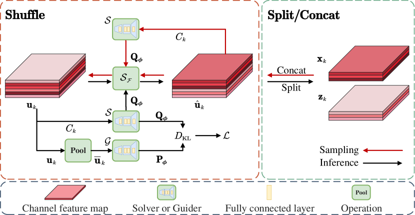
Figure 3: Schematic diagram of the inference and sampling process of the $\mathtt{Shuffle}$ and $\mathtt{Split}$ operations. $\mathcal{S}$, $\mathcal{G}$ and $\mathcal{S}_{\mathcal{F}}$ are our designed solver , guider and shuffler, respectively. For the channel feature maps of $\mathbf{u}_{k}$ and $\hat{\mathbf{u}}_{k}$, the darker the color, the greater the corresponding element in $\mathbf{Q}_{\boldsymbol{\phi}}$.

3.2 Entropy-informed Channel Weight Solver

The solver-$\mathcal{S}$ is designed to generate and assign channel-wise weights to each channel feature map of latent variables. In the inference process, weights are assigned to $\{\mathbf{u}_{k}\}_{k=1}^{K-1}$ before the $\mathtt{Split}$ operation. While in the sampling process, weights are assigned to $\{\hat{\mathbf{u}}_{k}\}_{k=1}^{K-1}$ after the $\mathtt{Concat}$ operation. This assignment is based on the evaluation of the richness and importance of feature information contained in each channel feature map of $\{\mathbf{u}_{k}\}_{k=1}^{K-1}$ or $\{\hat{\mathbf{u}}_{k}\}_{k=1}^{K-1}$. Such evaluation can be quantified by entropy according to the principles of information theory (see Section 4). In addition, $\mathcal{S}$ is initialized to assign equal weights to all channel feature maps.

However, if $\mathcal{S}$ takes $\{\mathbf{u}_{k}\}_{k=1}^{K-1}$ as input in the inference process, it cannot be reverted in the sampling process. This is due to the $\mathtt{Concat}$ operation being executed before the $\mathtt{Shuffle}$ operation in the sampling process, resulting in a shift of input from $\{\mathbf{u}_{k}\}_{k=1}^{K-1}$ to $\{\hat{\mathbf{u}}_{k}\}_{k=1}^{K-1}$ (see Fig. 3 for an explanatory overview). To cope with this problem, we find that simply taking the channel number of $\mathbf{u}_{k}$, i.e., $4C_{k}$, as input is an effective and flexible approach. Besides, this approach is naturally reversible at any scale. Note that the reversibility described here means that the input and output of $\mathcal{S}$ remain the same in both the inference and sampling processes.

Taking the $k$-th scale in the inference process as an example, $\mathcal{S}$ takes as input the latent variable $\mathbf{u}_{k}$, specifically focusing on the channel number $4C_{k}$ of $\mathbf{u}_{k}$. For ease of notation, we denote the input of $\mathcal{S}$ as $\mathbf{u}_{k}$, with the understanding that it is primarily the channel number $4C_{k}$ that is being utilized. With this in mind, the network structure of $\mathcal{S}$ is constructed as follows:

$$\begin{split}\mathbf{Q}_{\boldsymbol{\phi},\mathbf{u}_{k}}&=\mathcal{S}(\mathbf{u}_{k},\boldsymbol{W}_{\mathcal{S}})=\mathtt{Softmax}(\boldsymbol{W}_{\mathcal{S}}^{L_{\mathcal{S}}}\mathbf{h}_{L_{\mathcal{S}}-1}(\cdots\mathbf{h}_{1}(\boldsymbol{W}_{\mathcal{S}}^{1}\mathbf{u}_{k})))\end{split}$$ (8)

where $\mathbf{Q}_{\boldsymbol{\phi},\mathbf{u}_{k}}$ denotes the importance and richness quantification vector outputted by $\mathcal{S}$ given the input $\mathbf{u}_{k}$, $\boldsymbol{\phi}$ denotes the trainable parameters of the $\mathtt{Shuffle}$ operation. Note that $\mathbf{Q}_{\boldsymbol{\phi},\mathbf{u}_{k}}$ is at times compactly referred to as $\mathbf{Q}_{\boldsymbol{\phi}}$ for the sake of brevity throughout the paper. $\boldsymbol{W}_{\mathcal{S}}=\{\boldsymbol{W}_{\mathcal{S}}^{1},\boldsymbol{W}_{\mathcal{S}}^{2},\ldots,\boldsymbol{W}_{\mathcal{S}}^{L_{\mathcal{S}}}\}$ are parameters of $L_{\mathcal{S}}$ fully connected layers in $\mathcal{S}$. Here $\boldsymbol{W}_{\mathcal{S}}^{1}\in\mathbb{R}^{2C_{k}\times 1}$, $\boldsymbol{W}_{\mathcal{S}}^{l}\in\mathbb{R}^{2C_{k}\times 2C_{k}}$ ($l=2,3,\ldots,L_{\mathcal{S}}-1$) and $\boldsymbol{W}_{\mathcal{S}}^{L_{\mathcal{S}}}\in\mathbb{R}^{4C_{k}\times 2C_{k}}$. $\{\mathbf{h}_{l}\}_{l=1}^{L_{\mathcal{S}}-1}$ are activation functions. Note that the length of $\mathbf{Q}_{\boldsymbol{\phi},\mathbf{u}_{k}}$ and $\mathbf{Q}_{\boldsymbol{\phi},\hat{\mathbf{u}}_{k}}$ is $4C_{k}$, which is consistent with the channel number of $\mathbf{u}_{k}$ and $\hat{\mathbf{u}}_{k}$. In the inference process, $\hat{\mathbf{u}}_{k}$ is then split into two equal parts, $\mathbf{x}_{k}$ and $\mathbf{z}_{k}$.

However, a bottleneck problem lies in ensuring that $\mathcal{S}$ reasonably generates channel-wise weights to accurately imply the richness and importance of feature information contained in each channel feature map of $\mathbf{u}_{k}$ or $\hat{\mathbf{u}}_{k}$. In other words, the elements in $\mathbf{Q}_{\boldsymbol{\phi},\mathbf{u}_{k}}$ and $\mathbf{Q}_{\boldsymbol{\phi},\hat{\mathbf{u}}_{k}}$ corresponding to $\mathbf{x}_{k}$ should have greater values compared to those corresponding to $\mathbf{z}_{k}$. This indicates that $\mathbf{x}_{k}$ contains the more important channel feature maps of $\mathbf{u}_{k}$, while $\mathbf{z}_{k}$ contains the less important ones. It is still unclear since solver-$\mathcal{S}$ just takes the channel number of $\mathbf{u}_{k}$ and $\hat{\mathbf{u}}_{k}$ as input, which does not contain any feature information of $\mathbf{u}_{k}$ or $\hat{\mathbf{u}}_{k}$. Inspired by knowledge distillation[87], we introduce a feature information extraction network as the teacher to guide $\mathcal{S}$ to learn feature information in a proper way. We term the teacher network as Supervisory Weight Guider.

3.3 Supervisory Weight Guider

The guider-$\mathcal{G}$ is responsible for generating channel-wise weights by extracting feature information from each channel feature map of latent variables. Unlike $\mathcal{S}$, it is irreversible and is only available in the inference process.

In this paper, we construct the feature information extractor, i.e., the guider-$\mathcal{G}$, by refining global information by performing feature compression at the spatial level, which involves converting each two-dimensional channel feature map into a single real number. The widely adopted method for this is global average pooling [69]. While applied in $\mathcal{G}$, this method brings several advantages. Firstly, it is more robust to spatial transformations on the input data since it aggregates spatial information of the input data. Secondly, it does not introduce any trainable parameters, thus minimizing the risk of overfitting.

Formally, taking the $k$-th scale as an example, the supervisory weight guider-$\mathcal{G}$ takes $\mathbf{u}_{k}=[\mathbf{u}_{k}^{1},\mathbf{u}_{k}^{2},\ldots,\mathbf{u}_{k}^{4C_{k}}]^{T}$ with shape $[4C_{k},H_{k}/2,W_{k}/2]$ as input, where $\mathbf{u}_{k}^{c}\in\mathbb{R}^{\frac{H_{k}}{2}\times\frac{W_{k}}{2}}$ $(c=1,2,\ldots,4C_{k})$ is the $c$-th channel feature map of $\mathbf{u}_{k}$. Then the global average pooling process for each channel feature map can be described as:

$$\bar{u}_{k}^{c}=\mathtt{Pool}(\mathbf{u}_{k}^{c})=\frac{4}{H_{k}\times W_{k}}\sum_{a=1}^{H_{k}/2}\sum_{b=1}^{W_{k}/2}\mathbf{u}_{k}^{c}(a,b),$$ (9)

where $\mathtt{Pool}$ generates channel-wise feature $\bar{u}_{k}^{c}$. For ease of notation, $\mathbf{u}_{k}^{c}(a,b)$ is the value at $(a,b)$ of $\mathbf{u}_{k}^{c}$, $\bar{u}_{k}^{c}\in\mathbb{R}^{1\times 1}$ contains the global feature information of $\mathbf{u}_{k}^{c}$ and $\bar{\mathbf{u}}_{k}=[\bar{u}_{k}^{1},\bar{u}_{k}^{2},\ldots,\bar{u}_{k}^{4C_{k}}]^{T}\in\mathbb{R}^{4C_{k}\times 1\times 1}$ is the output of $\mathtt{Pool}(\mathbf{u}_{k})$.

After extracting the global information of all channel feature maps, $\mathcal{G}$ intermingles them with each other and outputs the weight vector $\mathbf{P}_{\boldsymbol{\phi},\mathbf{u}_{k}}$, which reveals the importance and richness of feature information among all channel feature maps. As defined above, the network structure of $\mathcal{G}$ can be constructed as follows:

$$\begin{split}\mathbf{P}_{\boldsymbol{\phi},\mathbf{u}_{k}}&=\mathcal{G}\left(\mathbf{u}_{k},\mathbf{W}_{\mathcal{G}}\right)=\mathtt{Softmax}(\mathbf{W}_{\mathcal{G}}^{L_{\mathcal{G}}}\mathbf{h}_{L_{\mathcal{G}}-1}(\cdots\mathbf{h}_{1}(\mathbf{W}_{\mathcal{G}}^{1}\mathtt{Pool}(\mathbf{u}_{k})))),\end{split}$$ (10)

where $\mathbf{P}_{\boldsymbol{\phi},\mathbf{u}_{k}}$ denotes the importance and richness quantification vector outputted by $\mathcal{G}$ given the input $\mathbf{u}_{k}$. Note that $\mathbf{P}_{\boldsymbol{\phi},\mathbf{u}_{k}}$ is at times compactly referred to as $\mathbf{P}_{\boldsymbol{\phi}}$ for the sake of brevity throughout the paper. $\boldsymbol{W}_{\mathcal{G}}=\{\boldsymbol{W}_{\mathcal{G}}^{1},\boldsymbol{W}_{\mathcal{G}}^{2},\ldots,\boldsymbol{W}_{\mathcal{G}}^{L_{\mathcal{G}}}\}$ are parameters of $L_{\mathcal{G}}$ fully connected layers in $\mathcal{G}$. Here $\boldsymbol{W}_{\mathcal{G}}^{1}\in\mathbb{R}^{\lfloor\frac{4C_{k}}{r}\rfloor\times 4C_{k}}$, $\boldsymbol{W}_{\mathcal{G}}^{l}\in\mathbb{R}^{\lfloor\frac{4C_{k}}{r}\rfloor\times\lfloor\frac{4C_{k}}{r}\rfloor}(l=2,3,\ldots,L_{\mathcal{G}}-1)$ and $\boldsymbol{W}_{\mathcal{G}}^{L_{\mathcal{G}}}\in\mathbb{R}^{4C_{k}\times\lfloor\frac{4C_{k}}{r}\rfloor}$. $r$ is the hyperparameter representing the reduction ratio of the first fully connected layer which is set to improve the efficiency. $\{\mathbf{h}_{l}\}_{l=1}^{L_{\mathcal{G}}-1}$ are activation functions.

3.4 Reversible and Entropy-informed Shuffle Operation

After the solver-$\mathcal{S}$ outputs channel-wise weights, the shuffler-$\mathcal{S}_{\mathcal{F}}$ shuffles the latent variables, such as $\mathbf{u}_{k}$ or $\hat{\mathbf{u}}_{k}$, across channel dimensions based on these weights. In the following part, we will summarize the $\mathtt{Shuffle}$ operation at $k$-th scale used in both the inference and sampling process.

In the inference process, $\mathcal{S}$ takes the channel number of $\mathbf{u}_{k}$, i.e., $C_{k}$, as input and outputs a $C_{k}$-dimensional vector $\mathbf{Q}_{\boldsymbol{\phi},\mathbf{u}_{k}}$. This vector serves as a directive for the $\mathtt{Shuffle}$ operation, yielding $\hat{\mathbf{u}}_{k}$. After shuffling, $\hat{\mathbf{u}}_{k}$ is split into two parts, $\mathbf{x}_{k}$ and $\mathbf{z}_{k}$, along the channel dimension.

In the sampling process, $\mathcal{S}$ inversely participates by again taking the channel number of $\hat{\mathbf{u}}_{k}$, i.e., $C_{k}$, as input but operates inversely in spirit. The output is the corresponding importance vector $\mathbf{Q}_{\boldsymbol{\phi},\hat{\mathbf{u}}_{k}}$. With the shuffled variable $\hat{\mathbf{u}}_{k}$, $\mathcal{S}$ reproduces the importance of each channel feature map of $\hat{\mathbf{u}}_{k}$, facilitating the reproduction of the original unshuffled variable $\mathbf{u}_{k}$. Notably, although the $\mathtt{Shuffle}$ operation does not reverse the transformation mathematically, it effectively allows for information restoration based on $\mathbf{Q}_{\boldsymbol{\phi},\hat{\mathbf{u}}_{k}}$.

3.5 Objective Function

As described above, $\mathbf{P}_{\boldsymbol{\phi},\mathbf{u}_{k}}$ is utilized to guide $\mathbf{Q}_{\boldsymbol{\phi},\mathbf{u}_{k}}$ to more effectively extract feature information contained in $\mathbf{u}_{k}$. And the sum of the components of $\mathbf{P}_{\boldsymbol{\phi},\mathbf{u}_{k}}$ and $\mathbf{Q}_{\boldsymbol{\phi},\mathbf{u}_{k}}$ is 1, which can be seen as the distribution of channel feature information. In this case, a generic way for letting $\mathbf{Q}_{\boldsymbol{\phi},\mathbf{u}_{k}}$ approach $\mathbf{P}_{\boldsymbol{\phi},\mathbf{u}_{k}}$ is to minimize the Kullback-Leibler (KL) divergence between these two weight vectors. Such KL divergence is defined as follows:

$$\text{KL}(\mathbf{P}_{\boldsymbol{\phi},\mathbf{u}_{k}}\|\mathbf{Q}_{\boldsymbol{\phi},\mathbf{u}_{k}};k)=\sum_{c=1}^{4C_{k}}\mathbf{P}_{\boldsymbol{\phi},\mathbf{u}_{k}}\left(c\right)\ln\frac{\mathbf{P}_{\boldsymbol{\phi},\mathbf{u}_{k}}\left(c\right)}{\mathbf{Q}_{\boldsymbol{\phi},\mathbf{u}_{k}}\left(c\right)},$$ (11)

where $\mathbf{P}_{\boldsymbol{\phi},\mathbf{u}_{k}}\left(c\right)$ and $\mathbf{Q}_{\boldsymbol{\phi},\mathbf{u}_{k}}\left(c\right)$ represent the $c$-th value of $\mathbf{P}_{\boldsymbol{\phi},\mathbf{u}_{k}}$ and $\mathbf{Q}_{\boldsymbol{\phi},\mathbf{u}_{k}}$, respectively.

In fact, our model training incorporates Eq. (11) to prevent $\mathbf{Q}_{\boldsymbol{\phi},\mathbf{u}_{k}}$ from becoming uniform over the channels. By focusing the $\mathcal{G}$’s training on maximizing the dataset’s likelihood, i.e., $-\log q_{\mathbf{\boldsymbol{\theta}}}(\mathbf{x})$, without the influence of the KL loss, each element in $\mathbf{P}_{\boldsymbol{\phi},\mathbf{u}_{k}}$ can reflect the richness and importance of the corresponding channel feature map’s feature information. Given the varying informational content across different channel feature maps, the elements within $\mathbf{P}_{\boldsymbol{\phi},\mathbf{u}_{k}}$ are intentionally non-uniform. Finally, under the effect of Eq. (11), the distribution $\mathbf{Q}_{\boldsymbol{\phi},\mathbf{u}_{k}}$ maintains a non-uniform distribution across channels.

This approach is strategic because an adept $\mathcal{G}$ is essential for guiding the $\mathcal{S}$ effectively. This guidance is crucial for the $\mathtt{Shuffle}$ operation to efficiently flow channel feature maps with incompletely extracted information to the next scale in our multi-scale architecture. Consequently, this process refines the final latent variables to better approximate a normal distribution. This alignment significantly improves the precision of the likelihood calculation for these latent variables, leading to a higher dataset likelihood. Furthermore, we also rigorously demonstrate the rationality and efficacy of the aforementioned approach from an information theory standpoint, as detailed in Section 4.

In practice, the Monte Carlo method is usually performed to estimate the KL divergence by sampling $\mathbf{u}_{k}$, which is realized by sampling $\mathbf{x}$ from $\mathcal{X}$. The total cumulative KL divergence is added to the vanilla loss function as in Eq. (4) to form the final objective function:

$$\mathcal{L}(\mathbf{x};\boldsymbol{\theta},\boldsymbol{\phi}) =\mathbb{E}_{\mathbf{x}\sim p(\mathbf{x})}\left[-\log q_{\mathbf{\boldsymbol{\theta}}}(\mathbf{x})+\lambda\sum_{k=1}^{K-1}\text{KL}(\mathbf{P}_{\boldsymbol{\phi},\mathbf{u}_{k}}\|\mathbf{Q}_{\boldsymbol{\phi},\mathbf{u}_{k}};k)\right]$$ (12)

$$\approx\frac{1}{|\mathcal{X}|}\sum_{\mathbf{x}\in\mathcal{X}}\left[-\log q_{\mathbf{\boldsymbol{\theta}}}(\mathbf{x})+\lambda\sum_{k=1}^{K-1}\sum_{c=1}^{4C_{k}}\mathbf{P}_{\boldsymbol{\phi},\mathbf{u}_{k}}\left(c\right)\ln\frac{\mathbf{P}_{\boldsymbol{\phi},\mathbf{u}_{k}}\left(c\right)}{\mathbf{Q}_{\boldsymbol{\phi},\mathbf{u}_{k}}\left(c\right)}\right],$$

where $\boldsymbol{\theta}$ and $\boldsymbol{\phi}$ denote the parameters of the vanilla flow-based model and the parameters of $\mathcal{S}$ along with $\mathcal{G}$ introduced by our method, respectively. $\lambda$ is a hyperparameter trading off between the two losses. $|\mathcal{X}|$ denotes the set size of $\mathcal{X}$.

The proposed training process is shown in Algorithm 1.

Algorithm 1 The training process for EIW-Flow

0:  datapoint $\mathbf{x}_{0}$ from dataset $\mathcal{X}$, epoch number $J$, scale number $K$, steps of flow $N$, hyperparameter $\lambda$.

  Initialize: the parameters $\boldsymbol{\theta}$ of vanilla model, the parameters $\boldsymbol{\phi}$ of solver-$\mathcal{S}$ and guider-$\mathcal{G}$ , total loss $\mathcal{L}=0$.

  for $j=1$ to $J$ do

     for $k=1$ to $K$ do

        %% Step 1: Shuffle and Split latent variables

        $\mathbf{u}_{k}=\mathtt{Squeeze}(\mathbf{f}_{k}^{N}\circ\cdots\circ\mathbf{f}_{k}^{2}\circ\mathbf{f}_{k}^{1}(\mathbf{x}_{k-1}))$

        $\mathbf{Q}_{\boldsymbol{\phi},\mathbf{u}_{k}}\leftarrow\mathcal{S}(\mathbf{u}_{k},\boldsymbol{W}_{\mathcal{S}})$  

        $\hat{\mathbf{u}}_{k}\leftarrow\mathcal{S}_{\mathcal{F}}(\mathbf{u}_{k},\mathbf{Q}_{\boldsymbol{\phi},\mathbf{u}_{k}})$

        $[\mathbf{x}_{k},\mathbf{z}_{k}]\leftarrow\mathtt{Split}(\hat{\mathbf{u}}_{k})$

        %% Step 2: Calculate the KL divergence

        $\mathbf{P}_{\boldsymbol{\phi},\mathbf{u}_{k}}\leftarrow\mathcal{G}\left(\mathbf{u}_{k},\mathbf{W}_{\mathcal{G}}\right)$

        $\mathcal{L}(\mathbf{x}_{0};\boldsymbol{\theta},\boldsymbol{\phi})\leftarrow\mathcal{L}(\mathbf{x}_{0};\boldsymbol{\theta},\boldsymbol{\phi})+\lambda\cdot\text{KL}(\mathbf{P}_{\boldsymbol{\phi},\mathbf{u}_{k}}\|\mathbf{Q}_{\boldsymbol{\phi},\mathbf{u}_{k}};k)$  

     end for

     $\mathcal{L}(\mathbf{x}_{0};\boldsymbol{\theta},\boldsymbol{\phi})\leftarrow\mathcal{L}(\mathbf{x}_{0};\boldsymbol{\theta},\boldsymbol{\phi})-\log q_{\boldsymbol{\theta}}(\mathbf{x}_{0})$  

     $[\boldsymbol{\theta},\boldsymbol{\phi}]\leftarrow\text{Adam}(\nabla_{\boldsymbol{\theta}}\mathcal{L}(\mathbf{x}_{0};\boldsymbol{\theta},\boldsymbol{\phi}),\nabla_{\boldsymbol{\phi}}\mathcal{L}(\mathbf{x}_{0};\boldsymbol{\theta},\boldsymbol{\phi}),\boldsymbol{\theta},\boldsymbol{\phi})$  

  end for

  the trained parameters $\boldsymbol{\theta}$ and $\boldsymbol{\phi}$.

4 Theorem Analysis

In Section 3, we have already detailed the mechanism of the $\mathtt{Shuffle}$ operation, and in Section 6 and 7, we will experimentally demonstrate its effectiveness. However, the reasons behind the effectiveness of the $\mathtt{Shuffle}$ operation remain unclear. Therefore, in this section, we will theoretically investigate the reasons behind the efficacy of $\mathtt{Shuffle}$ from an information theory perspective.

In this section, we qualitatively and quantitatively demonstrate that our proposed $\mathtt{Shuffle}$ operation actually ensures that the difference between the entropy of $\{\mathbf{x}_{k}\}_{k=1}^{K-1}$ and $\{\mathbf{z}_{k}\}_{k=1}^{K-1}$ within the EIW-Flow framework is greater than that in the vanilla model. We initiate with a qualitative exploration of the $\mathtt{Shuffle}$ operation through the lens of information theory, supported by Theorem 2 and Proposition 1, which provide insights into its entropy-increasing mechanisms. Building upon this theoretical foundation, we then quantitatively validate our claims through an extensive ablation study conducted across three benchmark datasets: CIFAR-10, CelebA, and MNIST.

NFs transform an observed variable in the data space with intractable complex distribution to a latent variable in the latent space with tractable simple distribution, such as the standard Gaussian distribution. This is guaranteed by the Central Limit Theorem (CLT). The CLT [78] states that under certain conditions, the distribution of sample means will converge to a Gaussian distribution as the sample size increases.

Besides, the Maximum Entropy Principle (MEP) [75] states that a random variable with a certain correlation matrix has maximum entropy when it follows a normal distribution. These two principles ensure that well-trained NFs usually tend to greater entropy in the inference process. While greater entropy means greater uncertainty, NFs can also be seen as a process which disrupts the structure of $\mathbf{x}$.

Theorem 1 (Maximum Entropy Principle, MEP[75])

Let $\mathbf{x}$ be a random variable with probability density distribution $p(\mathbf{x})$. If constraining the mean and variance of $\mathbf{x}$, the optimal probability distribution that maximizes the entropy $H(p)$ is the standard Gaussian distribution.

To analyze the nature of our $\mathtt{Shuffle}$ operation from the perspective of entropy theory, we design an ablation experiment on CIFAR-10, CelebA and MNIST datasets. We firstly approximate the entropy of each element of $\mathbf{x}_{k}$ and $\mathbf{z}_{k}$ $(k=1,2,\ldots,K-1)$ with Monte Carlo Estimation, namely:

$$H(p) =-\int_{\mathbb{R}}p(\mathbf{x})\log p(\mathbf{x})d\mathbf{x}\approx-\frac{1}{|\mathcal{X}|}\sum_{\mathbf{x}\in\mathcal{X}}\log p(\mathbf{x}).$$ (13)

Then we calculate the mathematical expectation of the entropy for each element of $\mathbf{x}_{k}$ and $\mathbf{z}_{k}$, which we term as the expected entropy of $\mathbf{x}_{k}$ and $\mathbf{z}_{k}$.

Definition 1 (Expected Entropy, E2)

Consider a random variable $\mathbf{x}$, its expected entropy is defined as follows:

$$\mathrm{E2}(\mathbf{x})\triangleq\frac{2}{C\times H\times W}\sum_{c=1}^{C/2}\sum_{a=1}^{H}\sum_{b=1}^{W}H(p(x^{c}(a,b))),$$ (14)

where $C$ and $[H,W]$ are the channel and spatial size of $\mathbf{x}$, $p(x^{c}(a,b))$ is the probability density distribution of $x^{c}(a,b)$, $x^{c}(a,b)$ denotes the value at $(a,b)$ of the $c$-th channel feature map of $\mathbf{x}$. A greater value of $\mathrm{E2}$ indicates that $\mathbf{x}$ is more likely to follow a standard Gaussian distribution.

Furthermore, to better compare vanilla architecture with our model, we define a new indicator named Relative Ratio of Expected Entropy ($\mathrm{R2E2}$).

Definition 2 (Relative Ratio of Expected Entropy, $\mathrm{R2E2}$)

Consider two random variables $\mathbf{x}$ and $\mathbf{z}$, their Relative Ratio of Expected Entropy is defined as follows:

$$\mathrm{R2E2}(\mathbf{x},\mathbf{z})\triangleq\frac{\mathrm{E2}(\mathbf{z})-\mathrm{E2}(\mathbf{x})}{\mathrm{E2}(\mathbf{x})}.$$ (15)

where $\mathrm{E2}(\cdot)$ is the expected entropy function as defined in Eq. 14. A greater value of $\mathrm{R2E2}$ indicates that the expected entropy of $\mathbf{z}$ is more greater than that of $\mathbf{x}$ without considering the magnitude, which also means $\mathbf{z}$ has less information.

According to MEP, if $\mathbf{z}_{k}$ truly follows a standard Gaussian distribution as assumed in NFs, $\mathrm{E2}(\mathbf{z}_{k})$ ought to be relatively greater, while the opposite is true for $\mathbf{x}_{k}$. In this case, the value of $\mathrm{R2E2}(\mathbf{x}_{k},\mathbf{z}_{k})$ should also be greater.

Theorem 2

The expected entropy of latent variable increases during the inference process of EIW-Flow.

Proof. EIW-Flow serves as a feature information extractor, progressively extracting feature information from input data. This results in the final latent variable follows a standard Gaussian distribution. Moreover, this also leads to an increase in the entropy value of latent variables in accordance with MEP. Specifically, the entropy of each element of the latent variables, such as $H(p(x^{c}(a,b)))$, also grows with the increase in scale number until they follow standard Gaussian distribution. Consequently, each term of the right hand side of Eq. (14) increases during the inference process. As a result, the expected entropy of latent variables naturally increases throughout the inference process according to the definition of expected entropy. $\Box$

Proposition 1

For $\forall k\in\{1,2,\ldots,K-1\}$, the $\mathrm{R2E2}$ between $\mathbf{x}_{k}$ and $\mathbf{z}_{k}$ for EIW-Flow is greater than that for vanilla normalizing flows.

Proof. As described in 3.2, the $\mathtt{Shuffle}$ operation propagates relatively information-rich channel feature maps of latent variables like $\mathbf{x}_{k}$ to the next scale. These channel feature maps have smaller entropy value based on MEP, indicating that $H(p(\mathbf{x}_{k}))$ is smaller than $H(p(\mathbf{z}_{k}))$ for all $k\in\{1,2,\ldots,K-1\}$. Additionally, some channel feature maps of $\mathbf{z}_{k}$ may contain more feature information of input data than that of $\mathbf{x}_{k}$ as shown in Fig. 1 when the $\mathtt{Shuffle}$ operation is not applied. This implies the difference between $\mathrm{E2}(\mathbf{z}_{k})$ and $\mathrm{E2}(\mathbf{x}_{k})$ is greater for EIW-Flow compared to the vanilla model, resulting in a greater $\mathrm{R2E2}(\mathbf{x}_{k},\mathbf{z}_{k})$. $\Box$

Proposition 1 states that channels with higher expected entropy will be used to form the final latent variable in EIW-Flow, i.e., $\mathrm{E2}(\mathbf{z}_{k})>\mathrm{E2}(\mathbf{x}_{k}),\forall k\in\{1,2,\ldots,K-1\}$. Specifically, according to the Maximum Entropy Principle described by Theorem 1, it can be inferred that under certain conditions, a random variable usually has lower information entropy when it contains richer and more important feature information. Specifically, the value of each element in $\mathbf{P}_{\boldsymbol{\phi}}$ is positively related to the richness and importance of the corresponding channel feature map’s feature information. Therefore, as the value of each element in $\mathbf{P}_{\boldsymbol{\phi}}$ increases, its information entropy decreases. By using Eq. (11) to train our model, the output $\mathbf{Q}_{\boldsymbol{\phi}}$ from solver-$\mathcal{S}$ can be progressively aligned with $\mathbf{P}_{\boldsymbol{\phi}}$ , thereby naturally identifying the elements with smaller values, i.e., higher entropy, along with their corresponding channel feature maps to form the final latent variable. The experimental results placed in Table 1 also demonstrate this proposition.

Our experimental results are presented in Table 1. We can observe that: 1) regardless of the dataset, the R2E2 after the $\mathtt{Shuffle}$ operation is much greater than that before the $\mathtt{Shuffle}$ operation; 2) for our model, the expected entropy of $\mathbf{z}_{k}$ is greater than that of $\mathbf{x}_{k}$, while for vanilla model there are some outliers; 3) the expected entropy of all $\mathbf{x}_{k}$ and $\mathbf{z}_{k}$ increase with increasing $k$. Combining (1) and (2), we know that our $\mathtt{Shuffle}$ operation actually leaves the channel feature maps, which have greater entropy and are more likely to follow a Gaussian distribution, to form the final latent variable. As for (3), in the assumptions of NFs, $\mathbf{z}_{k}$ follows a normal distribution while $\mathbf{x}_{k}$ follows a complicated unknown distribution. Hence the expected entropy of the former is greater than that of the latter. This shows that the experimental results are consistent with the assumptions of NFs.

Table 1: Expected Shannon information entropy before (vanilla) and after (our) our $\mathtt{Shuffle}$ operation on three image datasets.

dataset	stage	vanilla $\mathbf{x}_{k}$	vanilla $\mathbf{z}_{k}$	R2E2↑	our $\mathbf{x}_{k}$	our $\mathbf{z}_{k}$	R2E2↑	improvement rate
CIFAR-10 ($K=3$)	$k=1$ (training)	126.686	95.716	-0.244	91.616	253.140	1.763	82.25% ↑
	$k=2$ (training)	160.136	198.423	0.239	145.897	257.104	0.762	21.88% ↑
	$k=1$ (test)	112.938	122.165	0.082	103.350	205.970	0.993	111.1% ↑
	$k=2$ (test)	154.229	183.434	0.189	139.671	209.362	0.499	16.40% ↑
CelebA ($K=3$)	$k=1$ (training)	82.785	68.522	-0.172	62.996	184.765	1.933	122.4% ↑
	$k=2$ (training)	140.938	188.675	0.339	123.909	219.719	0.773	12.80% ↑
	$k=1$ (test)	80.844	63.133	-0.219	59.192	193.134	2.263	113.3% ↑
	$k=2$ (test)	144.818	175.831	0.214	127.732	208.120	0.629	19.39% ↑
MNIST ($K=2$)	$k=1$ (training)	159.195	163.357	0.026	155.329	162.525	0.046	7.692% ↑
	$k=1$ (test)	135.019	144.364	0.069	129.791	166.534	0.283	31.01% ↑

As a matter of fact, our $\mathtt{Shuffle}$ operation leaves the channel feature maps, whose corresponding elements in $\mathbf{Q}_{\boldsymbol{\phi}}$ are smaller, to form the final latent variable $\mathbf{z}$. Besides, a smaller value of $\mathbf{Q}_{\boldsymbol{\phi}}$ means containing less feature information of input data $\mathbf{x}$. Furthermore, less feature information leads to a greater Shannon information entropy, which is shown in our experimental results.

5 Related Works

Multi-scale architectures have been extensively investigated in deep generative models for latent space dimension reduction. Some initial works suggested splitting latent variables at earlier scales to distribute the loss function throughout flow models, leading to a substantial reduction in computation and memory [3, 88, 89]. However, the $\mathtt{Split}$ operation employed in the multi-scale architecture compromises the expressive power of NFs as it simply splits the high-dimensional variable into two lower-dimensional variables of equal size without considering the feature information of its input. [35] proposed to replace the $\mathtt{Split}$ operation with the wavelet transformation, which splits high-resolution variables into low-resolution variables and corresponding wavelet coefficients. This paper proposes to consider feature information contained in each channel feature map of high-dimensional variable during the $\mathtt{Split}$ operation. The schematic diagrams of the sampling process of our model and Wavelet Flow are shown in Fig. 4. In the sampling process, Wavelet Flow progressively transforms an image from low-resolution to high-resolution by predicting corresponding wavelet coefficients and applying wavelet transformation. Nevertheless, EIW-Flow (ours) progressively concatenates low-dimensional noisy variable with Gaussian noise to get high-dimensional variable and removes Gaussian noise from noisy variable with flow steps.

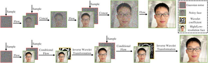
Figure 4: The sampling process of the multi-scale architectures used in EIW-Flow (top) and Wavelet Flow (bottom). The terms “conditional flow" and “inverse wavelet transformation" are introduced in [35]. “Sample" means sampling Gaussian noise from $\mathcal{N}(\mathbf{0},\mathbf{I})$. “Flow" represents flow steps in NFs.

6 Quantitative Evaluation

6.1 Density Estimation

In this section, we evaluate our model on three benchmark datasets: CIFAR-10 [12], CelebA [13] and ImageNet [14] (resized to $32\times 32$ and $64\times 64$ pixels) compared with several advanced generative models.

Since natural images are discretized, we apply a variational dequantization method [39] to obtain continuous data necessary for Normalizing Flows. We set the hyperparameter $\lambda=0.001$ to balance the optimization of the neural network $q_{\boldsymbol{\theta}}$ with the solver-$\mathcal{S}$. A too large $\lambda$ will result in neglecting the optimization of backbone neural network $q_{\boldsymbol{\theta}}$, while a too small $\lambda$ will prevent the solver-$\mathcal{S}$ from adequately approximating the guider-$\mathcal{G}$ we introduced, thus degrading the model to the original architecture as described in Section 2.3. We set the number of scales $K=3$ and the number of transformations $N=6$ in each scale so that the model is expressive enough and does not take too long to train. The learning rate is set to $0.001$ so that the model can converge well. We choose to use the optimizer of [42] to make a fair comparison with other models. We take advantage of the warm-up procedure described in [38]. All our experiments are conducted on a single Tesla-V100 GPU with $32$ GB memory.

Table 2 compares the generative performance of different NFs models. On these four datasets, i.e., CIFAR-10, CelebA, Imagenet32 and Imagenet64, our model achieves the best performance among NFs, which are $2.97$, $1.96$, $3.62$, $3.35$, respectively. The reported results are averaged over five runs with different random seeds.

Table 2: Negative log-likelihood (bits/dim) evaluation on image datasets. Asterisks (*) indicate that the model is best among all Normalizing Flows models. A short horizontal line (-) indicates that the corresponding paper did not experiment with this dataset.

Category	Model	CIFAR-10	CelebA	ImageNet32	ImageNet64
Normalizing Flows	REAL NVP [3]	3.49	3.02	4.28	3.98
	GLOW [6]	3.35	-	4.09	3.81
	Residual Flow [36]	3.28	-	4.01	3.78
	DenseFlow [38]	2.98	1.99	3.63	3.35
	Flow++ [39]	3.08	-	3.86	3.69
	Wavelet Flow [35]	-	-	4.08	3.78
	EIW-Flow (ours)	2.97∗	1.96∗	3.62∗	3.35∗

6.2 Experiments on MNIST dataset

Additionally, we conduct quantitative and qualitative experiments with the MNIST dataset, which is a simple yet meaningful dataset. Different from other datasets, we set the number of scale $K=2$ and the number of transformations $N=6$. The other hyperparameters and settings are the same as other three datasets.

We first compare our model with other NFs according to bits/dim and FID metrics. Results are presented in Table 3. Our model achieves the best performance among NFs for both bits/dim and FID, which are $0.89$ and $2.4$, respectively. This shows that our model is more suitable for generating high-fidelity handwritten digital images than other NFs.

Table 3: Evaluation of bits/dim and FID score on MNIST dataset. The “*" indicates that the model is optimal for all models compared. The “-" indicates that this model was not experimented on this dataset in the corresponding paper.

Model	bits/dim$\downarrow$	FID$\downarrow$
Residual Flow [36]	0.97	-
RNODE [72]	0.97	-
i-ResNet [50]	1.06	-
Sliced Iterative Generator [73]	1.34	4.5
GLF+perceptual loss [74]	-	5.8
EIW-Flow (ours)	0.89∗	2.4∗

We also generate handwritten digital images from our trained model by sampling $\mathbf{z}\sim N(\mathbf{0},\mathbf{I})$ in the latent space and reversing $\mathbf{z}$ according to the sampling process of EIW-Flow. The sampling process is described in Section 7.1 and the results are shown in Fig. 5. We can observe that the images in Fig. 5 have clear structures.

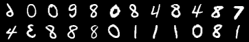
Figure 5: Random samples generated by EIW-Flow on MNIST dataset with temperature factor 0.5.

6.3 Computational Complexity

Since we have introduced a solver-$\mathcal{S}$ to automatically assign weights to channels at each scale, additional computational overhead will be inevitably added and thus limit the inference speed. Therefore, we use frames per second (FPS) on all four datasets to compare our trained model with vanilla model using the original architecture. For CIFAR-10 and ImageNet32, we set the batch size to $64$, while in other two cases it is set to $16$ due to memory limitations. The detailed results are shown in Table 4. The reported results are obtained on a single Tesla V-100 GPU. For CelebA and ImageNet64 datasets, our improved model adds less than $0.03$ seconds to vanilla one, which is insignificant in relation to the total elapsed time. As for the other two cases, we can observe that the increase in total elapsed time for EIW-Flow is negligible compared to the vanilla model. Moreover, the number of parameters of our model and vanilla model are 130.92 million and 130.65 million, respectively. Only $270$k parameters are added by solver-$\mathcal{S}$, indicating that the improvement in expressive power does not come from the deepening of our model.

Table 4: Comparison of Frames Per Second (FPS) and parameter size. The reported results are obtained on a single Tesla V-100 GPU with batch size 16 and are averaged over five runs.

Dataset	FPS$\uparrow$				Param Size (M)$\downarrow$
	Training set		Test set		our	vanilla
	our	vanilla	our	vanilla
CIFAR-10	1103	1088	1103	1088	130.92	130.65
CelebA	24	25	22	23	130.92	130.65
ImageNet32	102	105	88	90	130.92	130.65
ImageNet64	24	25	24	25	130.92	130.65

7 Qualitative Evaluation

7.1 Visual Quality

The analysis of visual quality is important as it is well-known that calculating log-likelihood is not necessarily indicative of visual fidelity [55]. In this part, we use the FID metric [54] to evaluate the visual quality of the samples generated by EIW-Flow. The FID score requires a large corpus of generated samples in order to provide an unbiased estimation. Hence, due to the memory limitation of our platform, we generate $50$k samples for all two datasets, which is also the default number in the calculation of FID score. Corresponding results can be seen in Table 5.

Table 5: Evaluation of FID score on two image datasets. Lower is better. Asterisks (*) indicate that the model is best among all Normalizing Flows models. A short horizontal line (-) indicates that the corresponding paper did not experiment with this dataset. We did not test it on ImageNet64 since the number of images needed to be stored exceed the memory limit.

Category	Model	CIFAR-10	CelebA	ImageNet32
Normalizing Flows	GLOW [6]	46.90	23.32	-
	DenseFlow [38]	34.90	17.1∗	38.5
	FCE [51]	37.30	12.21	-
	EIW-Flow (ours)	31.60∗	18.0	36.5∗

The generated ImageNet32 samples achieve a FID score of $36.5$, the CelebA samples achieve $18.0$ and when using the training dataset. When using the validation dataset, we achieve $34.3$ on CIFAR-10, $18.0$ on CelebA and $37.5$ on ImageNet32. Our model outperforms the majority of Normalizing Flows.

We also generate samples with our trained model. The sampling process is performed in an iteration of four steps: At $k$-th scale, we first sample $\mathbf{z}_{k}$ from the standard Gaussian distribution $\mathcal{N}(\boldsymbol{0},\mathbf{I})$. The shape of $\mathbf{z}_{k}$ is equal to $\mathbf{x}_{k}$ determined by scale number. Then we concatenate $\mathbf{z}_{k}$ with the input $\mathbf{x}_{k}$ to get the corresponding latent variable $\hat{\mathbf{u}}_{k}$. Next, we apply the inverse operation of our defined $\mathtt{Shuffle}$ operation followed by an $\mathtt{Unsqueeze}$ operation, which is the inversion of the $\mathtt{Squeeze}$ operation. Finally, the variable $\mathbf{u}_{k}$ is transformed by the inverse of flow steps $\{\mathbf{f}_{k}^{n}\}_{n=1}^{N}$ to get $\mathbf{x}_{k-1}$. The complete sampling process at the $k$-th scale is as follows:

$$\mathbf{z}_{k} \sim\mathcal{N}(\mathbf{0},\mathbf{I})$$ (16)

$$\hat{\mathbf{u}}_{k} =\mathtt{Concat}(\mathbf{x}_{k},\mathbf{z}_{k})$$ (17)

$$\mathbf{u}_{k} =\mathtt{Shuffle}^{-1}(\hat{\mathbf{u}}_{k})$$ (18)

$$\mathbf{x}_{k-1} =\mathbf{g}_{k}^{1}\circ\mathbf{g}_{k}^{2}\circ\cdots\circ\mathbf{g}_{k}^{N}(\mathtt{Unsqueeze}(\mathbf{u}_{k}))$$ (19)

where $\mathtt{Concat}$ and $\mathtt{Unsqueeze}$ are the inversion of the $\mathtt{Split}$ and $\mathtt{Squeeze}$ operations as described in Section 2.3. $\mathtt{Shuffle}^{-1}$ and $\mathbf{g}_{k}^{n}\triangleq(\mathbf{f}_{k}^{n})^{-1}$ denote the inverse process of the $\mathtt{Shuffle}$ operation and $\mathbf{f}_{k}^{n}$ as described in Fig. 3 and Section 2.3, respectively. Fig. 6a and Fig. 6b show images generated by the model trained on CelebA and ImageNet dataset respectively. For CelebA dataset, we take advantage of the reduced-temperature method [6] and set the factor $T=0.8$ to generate higher-quality samples.

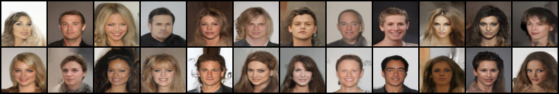
(a) CelebA ($64\times 64$ pixels).

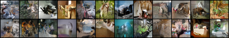
(b) ImageNet ($64\times 64$ pixels).

(c) CIFAR-10 ($32\times 32$ pixels).

Figure 6: Random samples generated by EIW-Flow on three image datasets, CelebA, ImageNet64 and CIFAR-10. The temperature factor of CelebA and CIFAR-10 are set to 0.8 and 0.95, respectively.

7.2 Interpolation Experiments

7.2.1 Comparison of Interpolation

We compare the effect of interpolation in data space and latent space. We first sample two points $\mathbf{x}_{0}$ and $\mathbf{x}_{1}$ from dataset, and interpolate them to obtain middle points $\mathbf{x}_{\alpha}$ as described in Section 7.2.2. Then we map $\mathbf{x}_{0}$ and $\mathbf{x}_{1}$ into the latent space to obtain $\mathbf{z}_{0}$ and $\mathbf{z}_{1}$. $\mathbf{z}_{\alpha}$ is obtained using the same interpolation method as $\mathbf{x}_{\alpha}$. Finally, we back-propagate them together to the data space and make a comparison with $\mathbf{x}_{\alpha}$. We test it using our model trained on the CelebA and CIFAR-10 datasets. Corresponding results are shown in Fig. 7a and Fig. 7b, respectively.

It can be seen that, in both CelebA and CIFAR-10 datasets, interpolation in the latent space tends to produce realistic images in the data space, whereas interpolation in the data space alone may cause unnatural effects (e.g., phantoms, overlaps, etc.). More importantly, this results demonstrates that our model learns a meaningful transformation between the latent space and the data space. In Fig. 7a, the model learns a transformation that manipulates the orientation of the head. While in Fig. 7b , the model has the ability to gradually turn a brown horse into a vibrant red car. It demonstrates that the latent space we have explored can be utilized in tasks that require more local face features such as 3D point clouds generation [93].

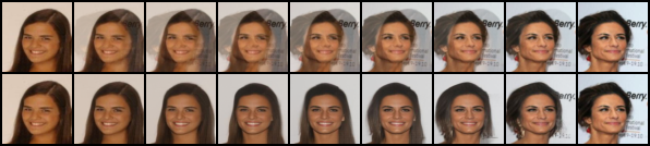
(a) CelebA ($64\times 64$ pixels).

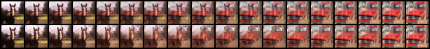
(b) CIFAR10 ($32\times 32$ pixels).

Figure 7: Comparison of interpolation on CelebA and CIFAR-10 datasets. The first row represents the results of interpolation in data space, i.e., $\mathbf{x}_{\alpha}$. While the second row represents the images that are transformed from $\mathbf{z}_{\alpha}$, corresponding to the results of interpolation in latent space.

7.2.2 Two-points Interpolation

We first randomly sample two datapoints $\mathbf{z}_{0}$ and $\mathbf{z}_{1}$ from the last scale. We then generate middle points $\mathbf{z}_{\alpha}$ by $\mathbf{z}_{\alpha}=(1-\alpha)\mathbf{z}_{1}+\alpha\mathbf{z}_{0}$. We back-propagate these variables together and interpolate at each scale using the same interpolation method. The CelebA and CIFAR-10 images are shown in Fig. 8a and Fig. 8b. We observe smooth interpolation between images belonging to distinct classes. This shows that the latent space we have explored can be potentially utilized for downstream tasks like image editing.

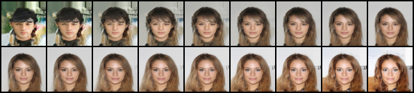
(a) CelebA ($64\times 64$ pixels).

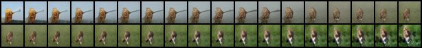
(b) CIFAR-10 ($32\times 32$ pixels).

Figure 8: Results of two-points interpolation on CelebA and CIFAR-10 datasets. The top left and bottom right images are endpoints $\mathbf{z}_{0}$ and $\mathbf{z}_{1}$. The other images corresponds to the middle points $\mathbf{z}_{\alpha}(0<\alpha<1)$. $\alpha$ increases gradually from the left to right and top to bottom.

7.3 Reconstruction

We first sample several datapoints $\mathbf{x}$ from the corresponding dataset, then reconstruct these points by $\hat{\mathbf{x}}=\mathbf{f}^{-1}(\mathbf{f}(\mathbf{x}))$ where $\mathbf{f}$ denotes the forward transformation of our model. We sample from the traning and test sets of CelebA and CIFAR-10. The results are shown in Fig. 9a and Fig. 9b. The top and bottom rows represent $\mathbf{x}$ and $\hat{\mathbf{x}}$, respectively. We observe that the reconstructed images $\hat{\mathbf{x}}$ are almost identical to the original images $\mathbf{x}$, which indicates the high reversibility of our model. Moreover, the results on the test set also indirectly demonstrate the comparable generalization performance of our model.

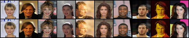
(a) CelebA ($64\times 64$ pixels).

(b) CIFAR-10 ($32\times 32$ pixels).

Figure 9: Reconstruction on CelebA and CIFAR-10. The first and second rows represent the original and the reconstructed images, respectively.

7.4 Semantic Manipulation

The semantic manipulation approach can be summarized as finding the path in the latent space that connects the two extremes of the same attribute [70]. In practice, the dataset is split into two subsets according to the value of pre-specified attribute. Then, the two subsets are mapped into the latent space and their corresponding average latent vectors can be calculated: $\mathbf{z}_{\mathrm{+}}$ and $\mathbf{z}_{\mathrm{-}}$. The resulting manipulation of a target image $\mathbf{x}_{\mathrm{target}}$ is obtained by adding a scaled manipulation vector $\mathbf{z}_{\mathrm{manipulation}}$ to its corresponding latent variable $\mathbf{z}_{\mathrm{target}}$:

$$\mathbf{z}_{\mathrm{final}}=\mathbf{z}_{\mathrm{target}}+\alpha\cdot\mathbf{z}_{\mathrm{manipulation}},$$ (20)

where $\mathbf{z}_{\mathrm{manipulation}}=\mathbf{z}_{\mathrm{+}}-\mathbf{z}_{\mathrm{-}}$ and $\alpha$ is the hyperparameter to control the manipulation effect.

We conduct experiments on CelebA dataset and present results on Fig. 10. Each row is made by interpolating the latent code of the target image along the vector corresponding to the attribute, with the middle image being the original image. For each row, the $\alpha$ increases by an equal difference from left to right, ranging from -2 to 2 for this experiment. Results show that EIW-Flow can make smooth and practically meaningful transformations of the features of the facial image.

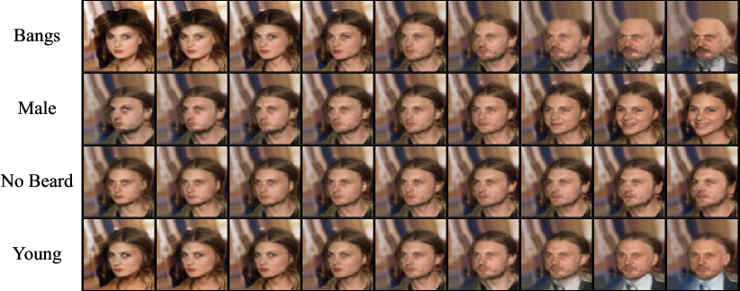
Figure 10: Semantic manipulation of attributes of a face image. Each row is made by interpolating the latent code of the target image along the vector corresponding to the attribute, with the middle image being the original image.

8 Ablation study

8.1 Effect of Temperature

We further conduct experiments to illustrate the effect of temperature annealing. A datapoint $\mathbf{z}$ in the latent space, with a given annealing parameter $T\in[0,1]$, can be formulated as $\mathbf{z}*T$. Specifically, there is no temperature annealing applied to $\mathbf{z}$ if $T=1$. We then back-propagate it to the data space to get the generated image. Results are shown in Fig. 11. It can be seen that taking value of annealing parameter $T$ from $0.8$ to $1$, i.e., four images on the right, can obtain realistic images and preserve face details from the original image. However, when $T<0.8$, the background and hair gradually becomes void as $T$ decreases.

Figure 11: Effect of temperature annealing on CelebA dataset. The images from left to right show the uniform increase of annealing parameter $T$ from $0.5$ to $1$. While $T=1$, there is no temperature annealing on latent variable.

8.2 Effect of $\mathtt{Shuffle}$ operation

To demonstrate the effectiveness and necessity of the $\mathtt{Shuffle}$ operation, we conduct an ablation experiment to compare the channel feature maps of latent variables before and after the $\mathtt{Shuffle}$ operation.

In Section 2.3, we state that $\mathbf{x}_{k}$ is propagated to the next scale, while the other half, $\mathbf{z}_{k}$, is left unchanged to form $\mathbf{z}$. However, the difference of channel feature maps between $\mathbf{x}_{k}$ and $\mathbf{z}_{k}$ has not yet been evaluated visually. Neither has the difference before and after the $\mathtt{Shuffle}$ operation. To explore these two questions, we conduct an ablation experiment according to the following procedure. For ease of notation, we continue to use $\mathbf{x}_{k}$ and $\mathbf{z}_{k}$ to indicate the first and second halves of both latent variables $\mathbf{u}_{k}$ and $\hat{\mathbf{u}}_{k}$, regargless of whether it is before or after the $\mathtt{Shuffle}$ operation.

Both before and after the $\mathtt{Shuffle}$ operation, we choose $l<C_{k}$ channel feature maps of $\mathbf{x}_{k}$ and $\mathbf{z}_{k}$, whose corresponding values in $\mathbf{Q}_{\boldsymbol{\phi}}$ are greater than others. Similarly, we can also choose $l$ channels with lower values in $\mathbf{Q}_{\boldsymbol{\phi}}$. In this experiment, we set $l=10$ for a better visualization. Results are shown in Fig. 12. In this figure, the terms “vanilla" and “ours" are used to refer to the results before and after the $\mathtt{Shuffle}$ operation, respectively. These two terms also corresponds to the results without and with the $\mathtt{Shuffle}$ operation, respectively.

We can observe that the channel feature maps of $\mathbf{z}_{k}$ before the $\mathtt{Shuffle}$ operation (i.e. vanilla $\mathbf{z}_{k}$) still contain some face structure information, while corresponding channel feature maps of $\mathbf{x}_{k}$ (i.e. vanilla $\mathbf{x}_{k}$) seem more like Gaussian noise. This result contradicts with the purpose of a multi-scale architecture, i.e. $\mathbf{z}_{k}$ ought to follow a multivariate Gaussian distribution and $\mathbf{x}_{k}$ should contain some feature information. However, the results after the $\mathtt{Shuffle}$ operation are contrary to the previous ones. This implies the channel feature maps of $\mathbf{x}_{k}$ contain more face structure information and $\mathbf{z}_{k}$ are more likely to follow a multivariate Gaussian distribution. This provides evidence to demonstrate the effectiveness of our designed $\mathtt{Shuffle}$ operation.

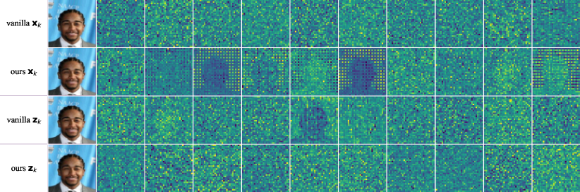
Figure 12: Effectiveness of $\mathtt{Shuffle}$ operation on CelebA dataset. The first and third rows represent the channel feature maps before the $\mathtt{Shuffle}$ operation, and the other two rows represent the channel feature maps after the $\mathtt{Shuffle}$ operation. The terms $\mathbf{x}_{k}$ and $\mathbf{z}_{k}$ indicate the first and second halves of both latent variables $\mathbf{u}_{k}$ and $\hat{\mathbf{u}}_{k}$, see Section 8.2 for details.

8.3 Effect of hyperparameter $\lambda$

In Eq. (LABEL:eq:final-loss), we introduce a hyperparameter, $\lambda$, to trade off between vanilla and our introduced loss. If $\lambda$ is too small, the solver-$\mathcal{S}$ may not approximate guider-$\mathcal{G}$. Specifically, $\mathcal{G}$ stops working when $\lambda=0$. This can lead to disorganised and chaotic shuffling of latent variables by the $\mathtt{Shuffle}$ operation. On the other hand, if $\lambda$ is relatively large, the effect of the likelihood loss function on EIW-Flow may be limited, resulting in decreased expressive power. Therefore, choosing an appropriate $\lambda$ is essential for training EIW-Flow. To find a better $\lambda$, we perform an ablation experiment on the CIFAR-10 dataset for NFs like EIW-Flow. Additionally, we have also applied the $\mathtt{Shuffle}$ operation to Continous Normalizing Flows like FFJORD [86] on CIFAR-10 dataset. This extended ablation experiment is conducted with different $\lambda$ to explore the effect of $\lambda$ for various types of NFs. The corresponding results are presented in Table 6. Note that the results of CNFs were derived after training for 50 epochs, which took approximately seven days to complete on a single Titan V GPU. For NFs, an appropriate $\lambda=1e-3$ gets the best performance 2.97, while a larger or smaller $\lambda$ may compromise performance. For CNFs, $\lambda=1e-4$ is the best choice to get a better performance.

Table 6: Ablation experiment for hyperparameter $\lambda$ on CIFAR-10 dataset for various types of NFs, i.e., Normalizing Flows and Continuous Normalizing Flows.

Normalizing Flows		Continuous Normalizing Flows
hyperparameter $\lambda$	bits/dim$\downarrow$	hyperparameter $\lambda$	bits/dim$\downarrow$
$1e-1$	3.092	$1e-1$	3.5025
$1e-2$	3.021	$1e-2$	3.5097
$1e-3$	2.97	$1e-3$	3.5024
$1e-4$	3.015	$1e-4$	3.4981

9 Limitations and Future Work

While our study has yielded valuable insights, it’s important to acknowledge its limitations. The dataset used lacks diversity and size, potentially limiting the generalizability of our findings. Additionally, the computational complexity of our model may impede real-time application, necessitating further optimization efforts for efficiency. Moving forward, it’s essential for future research to address these limitations. This entails leveraging larger and more diverse datasets to validate the efficacy of the $\mathtt{Shuffle}$ operation and optimizing the model for real-time applications. Moreover, conducting comprehensive comparative studies with alternative techniques, such as direct association of logits with model parameters for $\mathbf{Q}_{\phi}$, will be essential to validate our approach’s distinctiveness.

10 Conclusion

In this paper, we introduce a reversible and regularized $\mathtt{Shuffle}$ operation and integrate it into vanilla multi-scale architecture. The resulting flow-based generative model is called Entropy-informed Weighting Channel Normalizing Flow (EIW-Flow). The $\mathtt{Shuffle}$ operation is composed of three distinct components: solver, guider and shuffler. We demonstrate the efficacy of the $\mathtt{Shuffle}$ operation from the perspective of entropy using Central Limit Theorem and the Maximum Entropy Principle. The quantitative and qualitative experiments show that EIW-Flow results in better density estimation and generates high-quality images compared with previous state-of-the-art deep generative models. Besides, we compare the computational complexity with the vanilla architecture and observe that only negligible additional computational overhead is added by our model. Furthermore, we also conduct different types of ablation experiments to explore the effect of hyperparameters and the $\mathtt{Shuffle}$ operation.

References

- [1] S. Ruder, An overview of gradient descent optimization algorithms, arXiv preprint arXiv:1609.04747 (2016).
- [2] L. Dinh, D. Krueger, Y. Bengio, Nice: Non-linear independent components estimation, arXiv preprint arXiv:1410.8516 (2014).
- [3] L. Dinh, J. Sohl-Dickstein, S. Bengio, Density estimation using real nvp, arXiv preprint arXiv:1605.08803 (2016).
- [4] J. Hu, L. Shen, G. Sun, Squeeze-and-excitation networks, in: Proceedings of the IEEE conference on computer vision and pattern recognition, 2018, pp. 7132–7141.
- [5] I. Goodfellow, J. Pouget-Abadie, M. Mirza, B. Xu, D. Warde-Farley, S. Ozair, A. Courville, Y. Bengio, Generative adversarial nets, Advances in neural information processing systems 27 (2014).
- [6] D. P. Kingma, P. Dhariwal, Glow: Generative flow with invertible 1x1 convolutions, Advances in neural information processing systems 31 (2018).
- [7] D. P. Kingma, M. Welling, An introduction to variational autoencoders, arXiv preprint arXiv:1906.02691 (2019).
- [8] Y. Zhang, K. Li, K. Li, L. Wang, B. Zhong, Y. Fu, Image super-resolution using very deep residual channel attention networks, in: Proceedings of the European conference on computer vision (ECCV), 2018, pp. 286–301.
- [9] S. Woo, J. Park, J.-Y. Lee, I. S. Kweon, Cbam: Convolutional block attention module, in: Proceedings of the European conference on computer vision (ECCV), 2018, pp. 3–19.
- [10] S. Liu, L. Qi, H. Qin, J. Shi, J. Jia, Path aggregation network for instance segmentation, in: Proceedings of the IEEE conference on computer vision and pattern recognition, 2018, pp. 8759–8768.
- [11] A. Bhattacharyya, S. Mahajan, M. Fritz, B. Schiele, S. Roth, Normalizing flows with multi-scale autoregressive priors, in: Proceedings of the IEEE/CVF Conference on Computer Vision and Pattern Recognition, 2020, pp. 8415–8424.
- [12] A. Krizhevsky, G. Hinton, et al., Learning multiple layers of features from tiny images (2009).
- [13] Z. Liu, P. Luo, X. Wang, X. Tang, Deep learning face attributes in the wild, in: Proceedings of the IEEE international conference on computer vision, 2015, pp. 3730–3738.
- [14] O. Russakovsky, J. Deng, H. Su, J. Krause, S. Satheesh, S. Ma, Z. Huang, A. Karpathy, A. Khosla, M. Bernstein, et al., Imagenet large scale visual recognition challenge, International journal of computer vision 115 (3) (2015) 211–252.
- [15] J. Ho, A. Jain, P. Abbeel, Denoising diffusion probabilistic models, Advances in Neural Information Processing Systems 33 (2020) 6840–6851.
- [16] D. Kim, S. Shin, K. Song, W. Kang, I.-C. Moon, Score matching model for unbounded data score, arXiv preprint arXiv:2106.05527 (2021).
- [17] A. Q. Nichol, P. Dhariwal, Improved denoising diffusion probabilistic models, in: International Conference on Machine Learning, PMLR, 2021, pp. 8162–8171.
- [18] D. P. Kingma, T. Salimans, B. Poole, J. Ho, Variational diffusion models, arXiv preprint arXiv:2107.00630 (2021).
- [19] A. Van den Oord, N. Kalchbrenner, L. Espeholt, O. Vinyals, A. Graves, et al., Conditional image generation with pixelcnn decoders, Advances in neural information processing systems 29 (2016).
- [20] A. Van Oord, N. Kalchbrenner, K. Kavukcuoglu, Pixel recurrent neural networks, in: International conference on machine learning, PMLR, 2016, pp. 1747–1756.
- [21] T. Salimans, A. Karpathy, X. Chen, D. P. Kingma, Pixelcnn++: Improving the pixelcnn with discretized logistic mixture likelihood and other modifications, arXiv preprint arXiv:1701.05517 (2017).
- [22] N. Parmar, A. Vaswani, J. Uszkoreit, L. Kaiser, N. Shazeer, A. Ku, D. Tran, Image transformer, in: International Conference on Machine Learning, PMLR, 2018, pp. 4055–4064.
- [23] X. Chen, N. Mishra, M. Rohaninejad, P. Abbeel, Pixelsnail: An improved autoregressive generative model, in: International Conference on Machine Learning, PMLR, 2018, pp. 864–872.
- [24] J. Menick, N. Kalchbrenner, Generating high fidelity images with subscale pixel networks and multidimensional upscaling, arXiv preprint arXiv:1812.01608 (2018).
- [25] A. Roy, M. Saffar, A. Vaswani, D. Grangier, Efficient content-based sparse attention with routing transformers, Transactions of the Association for Computational Linguistics 9 (2021) 53–68.
- [26] K. Gregor, F. Besse, D. Jimenez Rezende, I. Danihelka, D. Wierstra, Towards conceptual compression, Advances In Neural Information Processing Systems 29 (2016).
- [27] A. Vahdat, W. Macready, Z. Bian, A. Khoshaman, E. Andriyash, Dvae++: Discrete variational autoencoders with overlapping transformations, in: International Conference on Machine Learning, PMLR, 2018, pp. 5035–5044.
- [28] L. Maaløe, M. Fraccaro, V. Liévin, O. Winther, Biva: A very deep hierarchy of latent variables for generative modeling, Advances in neural information processing systems 32 (2019).
- [29] S. Sinha, A. B. Dieng, Consistency regularization for variational auto-encoders, Advances in Neural Information Processing Systems 34 (2021).
- [30] X. Ma, X. Kong, S. Zhang, E. Hovy, Macow: Masked convolutional generative flow, Advances in Neural Information Processing Systems 32 (2019).
- [31] D. Nielsen, P. Jaini, E. Hoogeboom, O. Winther, M. Welling, Survae flows: Surjections to bridge the gap between vaes and flows, Advances in Neural Information Processing Systems 33 (2020) 12685–12696.
- [32] A. Vahdat, J. Kautz, Nvae: A deep hierarchical variational autoencoder, Advances in Neural Information Processing Systems 33 (2020) 19667–19679.
- [33] H. Sadeghi, E. Andriyash, W. Vinci, L. Buffoni, M. H. Amin, Pixelvae++: Improved pixelvae with discrete prior, arXiv preprint arXiv:1908.09948 (2019).
- [34] A. Razavi, A. v. d. Oord, B. Poole, O. Vinyals, Preventing posterior collapse with delta-vaes, arXiv preprint arXiv:1901.03416 (2019).
- [35] J. J. Yu, K. G. Derpanis, M. A. Brubaker, Wavelet flow: Fast training of high resolution normalizing flows, Advances in Neural Information Processing Systems 33 (2020) 6184–6196.
- [36] R. T. Chen, J. Behrmann, D. K. Duvenaud, J.-H. Jacobsen, Residual flows for invertible generative modeling, Advances in Neural Information Processing Systems 32 (2019).
- [37] Y. Perugachi-Diaz, J. Tomczak, S. Bhulai, Invertible densenets with concatenated lipswish, Advances in Neural Information Processing Systems 34 (2021).
- [38] M. Grcić, I. Grubišić, S. Šegvić, Densely connected normalizing flows, Advances in Neural Information Processing Systems 34 (2021).
- [39] J. Ho, X. Chen, A. Srinivas, Y. Duan, P. Abbeel, Flow++: Improving flow-based generative models with variational dequantization and architecture design, in: International Conference on Machine Learning, PMLR, 2019, pp. 2722–2730.
- [40] C.-W. Huang, L. Dinh, A. Courville, Augmented normalizing flows: Bridging the gap between generative flows and latent variable models, arXiv preprint arXiv:2002.07101 (2020).
- [41] J. Chen, C. Lu, B. Chenli, J. Zhu, T. Tian, Vflow: More expressive generative flows with variational data augmentation, in: International Conference on Machine Learning, PMLR, 2020, pp. 1660–1669.
- [42] D. P. Kingma, J. Ba, Adam: A method for stochastic optimization, arXiv preprint arXiv:1412.6980 (2014).
- [43] G. Ostrovski, W. Dabney, R. Munos, Autoregressive quantile networks for generative modeling, in: International Conference on Machine Learning, PMLR, 2018, pp. 3936–3945.
- [44] Z. Xiao, K. Kreis, J. Kautz, A. Vahdat, Vaebm: A symbiosis between variational autoencoders and energy-based models, arXiv preprint arXiv:2010.00654 (2020).
- [45] G. Parmar, D. Li, K. Lee, Z. Tu, Dual contradistinctive generative autoencoder, in: Proceedings of the IEEE/CVF Conference on Computer Vision and Pattern Recognition, 2021, pp. 823–832.
- [46] J. Aneja, A. Schwing, J. Kautz, A. Vahdat, A contrastive learning approach for training variational autoencoder priors, arXiv preprint arXiv:2010.02917 (2020).
- [47] A. Radford, L. Metz, S. Chintala, Unsupervised representation learning with deep convolutional generative adversarial networks, arXiv preprint arXiv:1511.06434 (2015).
- [48] I. Gulrajani, F. Ahmed, M. Arjovsky, V. Dumoulin, A. C. Courville, Improved training of wasserstein gans, Advances in neural information processing systems 30 (2017).
- [49] S. Zhao, Z. Liu, J. Lin, J.-Y. Zhu, S. Han, Differentiable augmentation for data-efficient gan training, Advances in Neural Information Processing Systems 33 (2020) 7559–7570.
- [50] J. Behrmann, W. Grathwohl, R. T. Chen, D. Duvenaud, J.-H. Jacobsen, Invertible residual networks, in: International Conference on Machine Learning, PMLR, 2019, pp. 573–582.
- [51] R. Gao, E. Nijkamp, D. P. Kingma, Z. Xu, A. M. Dai, Y. N. Wu, Flow contrastive estimation of energy-based models, in: Proceedings of the IEEE/CVF Conference on Computer Vision and Pattern Recognition, 2020, pp. 7518–7528.
- [52] D. P. Kingma, M. Welling, Auto-encoding variational bayes, arXiv preprint arXiv:1312.6114 (2013).
- [53] P. Ghosh, M. S. Sajjadi, A. Vergari, M. Black, B. Schölkopf, From variational to deterministic autoencoders, arXiv preprint arXiv:1903.12436 (2019).
- [54] M. Heusel, H. Ramsauer, T. Unterthiner, B. Nessler, S. Hochreiter, Gans trained by a two time-scale update rule converge to a local nash equilibrium, Advances in neural information processing systems 30 (2017).
- [55] L. Theis, A. v. d. Oord, M. Bethge, A note on the evaluation of generative models, arXiv preprint arXiv:1511.01844 (2015).
- [56] S. Dieleman, A. van den Oord, K. Simonyan, The challenge of realistic music generation: modelling raw audio at scale, Advances in Neural Information Processing Systems 31 (2018).
- [57] R. Prenger, R. Valle, B. Catanzaro, Waveglow: A flow-based generative network for speech synthesis, in: ICASSP 2019-2019 IEEE International Conference on Acoustics, Speech and Signal Processing (ICASSP), IEEE, 2019, pp. 3617–3621.
- [58] G. Yang, X. Huang, Z. Hao, M.-Y. Liu, S. Belongie, B. Hariharan, Pointflow: 3d point cloud generation with continuous normalizing flows, in: Proceedings of the IEEE/CVF International Conference on Computer Vision, 2019, pp. 4541–4550.
- [59] E. Nalisnick, A. Matsukawa, Y. W. Teh, D. Gorur, B. Lakshminarayanan, Hybrid models with deep and invertible features, in: International Conference on Machine Learning, PMLR, 2019, pp. 4723–4732.
- [60] D. P. Kingma, T. Salimans, R. Jozefowicz, X. Chen, I. Sutskever, M. Welling, Improved variational inference with inverse autoregressive flow, Advances in neural information processing systems 29 (2016).
- [61] X. Ma, X. Kong, S. Zhang, E. Hovy, Decoupling global and local representations via invertible generative flows, arXiv preprint arXiv:2004.11820 (2020).
- [62] R. Salakhutdinov, Learning deep generative models, Annual Review of Statistics and Its Application 2 (2015) 361–385.
- [63] J. Xu, H. Li, S. Zhou, An overview of deep generative models, IETE Technical Review 32 (2) (2015) 131–139.
- [64] M. Ranzato, J. Susskind, V. Mnih, G. Hinton, On deep generative models with applications to recognition, in: CVPR 2011, IEEE, 2011, pp. 2857–2864.
- [65] G. Papamakarios, E. Nalisnick, D. J. Rezende, S. Mohamed, B. Lakshminarayanan, Normalizing flows for probabilistic modeling and inference, Journal of Machine Learning Research 22 (57) (2021) 1–64.
- [66] A. F. Agarap, Deep learning using rectified linear units (relu), arXiv preprint arXiv:1803.08375 (2018).
- [67] Y. Lu, N. Kasabov, G. Lu, Multi-view geometry consistency network for facial micro-expression recognition from various perspectives, in: 2021 International Joint Conference on Neural Networks (IJCNN), IEEE, 2021, pp. 1–8.
- [68] P. Terhörst, M. Ihlefeld, M. Huber, N. Damer, F. Kirchbuchner, K. Raja, A. Kuijper, Qmagface: Simple and accurate quality-aware face recognition, arXiv preprint arXiv:2111.13475 (2021).
- [69] T.-Y. Hsiao, Y.-C. Chang, H.-H. Chou, C.-T. Chiu, Filter-based deep-compression with global average pooling for convolutional networks, Journal of Systems Architecture 95 (2019) 9–18.
- [70] A. Valenzuela, C. Segura, F. Diego, V. Gómez, Expression transfer using flow-based generative models, in: Proceedings of the IEEE/CVF Conference on Computer Vision and Pattern Recognition, 2021, pp. 1023–1031.
- [71] J. Gou, B. Yu, S. J. Maybank, D. Tao, Knowledge distillation: A survey, International Journal of Computer Vision 129 (6) (2021) 1789–1819.
- [72] C. Finlay, J.-H. Jacobsen, L. Nurbekyan, A. Oberman, How to train your neural ode: the world of jacobian and kinetic regularization, in: International conference on machine learning, PMLR, 2020, pp. 3154–3164.
- [73] B. Dai, U. Seljak, Sliced iterative normalizing flows, arXiv preprint arXiv:2007.00674 (2020).
- [74] Z. Xiao, Q. Yan, Y. Amit, Generative latent flow, arXiv preprint arXiv:1905.10485 (2019).
- [75] J. Shore, R. Johnson, Axiomatic derivation of the principle of maximum entropy and the principle of minimum cross-entropy, IEEE Transactions on information theory 26 (1) (1980) 26–37.
- [76] K. He, X. Zhang, S. Ren, J. Sun, Deep residual learning for image recognition, in: Proceedings of the IEEE conference on computer vision and pattern recognition, 2016, pp. 770–778.
- [77] S. Du, Y. Luo, W. Chen, J. Xu, D. Zeng, To-flow: Efficient continuous normalizing flows with temporal optimization adjoint with moving speed, in: Proceedings of the IEEE/CVF Conference on Computer Vision and Pattern Recognition, 2022, pp. 12570–12580.
- [78] M. Rosenblatt, A central limit theorem and a strong mixing condition, Proceedings of the national Academy of Sciences 42 (1) (1956) 43–47.
- [79] H. P. Das, P. Abbeel, C. J. Spanos, Likelihood contribution based multi-scale architecture for generative flows, arXiv preprint arXiv:1908.01686 (2019).
- [80] L. Yang, G. Karniadakis, Potential flow generator with l2; optimal transport regularity for generative models., IEEE Transactions on Neural Networks and Learning Systems 33 (2) (2022) 528–538.
- [81] R. Liang, Y. Li, J. Zhou, X. Li, Stglow: a flow-based generative framework with dual-graphormer for pedestrian trajectory prediction, IEEE transactions on neural networks and learning systems (2023).
- [82] S. T. Radev, U. K. Mertens, A. Voss, L. Ardizzone, U. Kothe, Bayesflow: Learning complex stochastic models with invertible neural networks, IEEE transactions on neural networks and learning systems 33 (4) (2022) 1452–1466.
- [83] H. Tu, Z. Yang, J. Yang, L. Zhou, Y. Huang, Fet-lm: Flow-enhanced variational autoencoder for topic-guided language modeling, IEEE Transactions on Neural Networks and Learning Systems (2023).
- [84] J.-T. Chien, S.-J. Huang, Learning flow-based disentanglement, IEEE Transactions on Neural Networks and Learning Systems (2022).
- [85] Y.-J. Yeo, Y.-G. Shin, S. Park, S.-J. Ko, Simple yet effective way for improving the performance of gan, IEEE Transactions on Neural Networks and Learning Systems 33 (4) (2021) 1811–1818.
- [86] W. Grathwohl, R. T. Chen, J. Bettencourt, I. Sutskever, D. Duvenaud, Ffjord: Free-form continuous dynamics for scalable reversible generative models, arXiv preprint arXiv:1810.01367 (2018).
- [87] C. Tan, J. Liu, Improving knowledge distillation with a customized teacher, IEEE Transactions on Neural Networks and Learning Systems (2022).
- [88] K. Jiang, Z. Wang, P. Yi, C. Chen, G. Wang, Z. Han, J. Jiang, Z. Xiong, Multi-scale hybrid fusion network for single image deraining, IEEE Transactions on Neural Networks and Learning Systems (2021).
- [89] Y. Hong, H. Pan, Y. Jia, W. Sun, H. Gao, Resdnet: Efficient dense multi-scale representations with residual learning for high-level vision tasks, IEEE Transactions on Neural Networks and Learning Systems (2022).
- [90] X. Hu, X. Wei, J. Sun, A noising-denoising framework for point cloud upsampling via normalizing flows, Pattern Recognition 140 (2023) 109569.
- [91] Y. Zha, F. Li, P. Zhang, W. Huang, Conditional invertible image re-scaling, Pattern Recognition 139 (2023) 109459.
- [92] Y. Cai, L. Li, A. Abel, X. Zhu, D. Wang, Maximum gaussianality training for deep speaker vector normalization, Pattern Recognition 145 (2024) 109977.
- [93] P. Li, X. Liu, J. Huang, D. Xia, J. Yang, Z. Lu, Progressive generation of 3d point clouds with hierarchical consistency, Pattern Recognition 136 (2023) 109200.
- [94] D. Gammelli, F. Rodrigues, Recurrent flow networks: A recurrent latent variable model for density estimation of urban mobility, Pattern Recognition 129 (2022) 108752.