In this section, we setup the framework for dealing with signatures of semimartingales. We not only collect some (well-known) properties of finite linear combinations of signature elements, refer also to the first sections in [5 , 12 , 26 ] , but we also introduce and study the resolvent object in Section 2.2
2.1 Tensor algebra
Let d ∈ ℕ 𝑑 ℕ d\in\mathbb{N} ⊗ tensor-product \otimes ℝ d superscript ℝ 𝑑 \mathbb{R}^{d} ( x ⊗ y ⊗ z ) i j k = x i y j z k subscript tensor-product 𝑥 𝑦 𝑧 𝑖 𝑗 𝑘 subscript 𝑥 𝑖 subscript 𝑦 𝑗 subscript 𝑧 𝑘 (x\otimes y\otimes z)_{ijk}=x_{i}y_{j}z_{k} i , j , k = 1 , … , d formulae-sequence 𝑖 𝑗 𝑘
1 … 𝑑
i,j,k=1,\dots,d x , y , z ∈ ℝ d 𝑥 𝑦 𝑧
superscript ℝ 𝑑 x,y,z\in\mathbb{R}^{d} n ≥ 1 𝑛 1 n\geq 1 ( ℝ d ) ⊗ n superscript superscript ℝ 𝑑 tensor-product absent 𝑛 (\mathbb{R}^{d})^{\otimes n} n 𝑛 n ( ℝ d ) ⊗ 0 = ℝ superscript superscript ℝ 𝑑 tensor-product absent 0 ℝ (\mathbb{R}^{d})^{\otimes 0}=\mathbb{R} T ( ( ℝ d ) ) 𝑇 superscript ℝ 𝑑 T((\mathbb{R}^{d})) ℝ d superscript ℝ 𝑑 \mathbb{R}^{d}
T ( ( ℝ d ) ) := { ℓ = ( ℓ n ) n = 0 ∞ : ℓ n ∈ ( ℝ d ) ⊗ n } . assign 𝑇 superscript ℝ 𝑑 conditional-set bold-ℓ superscript subscript superscript bold-ℓ 𝑛 𝑛 0 superscript bold-ℓ 𝑛 superscript superscript ℝ 𝑑 tensor-product absent 𝑛 T((\mathbb{R}^{d})):=\left\{\bm{\ell}=(\bm{\ell}^{n})_{n=0}^{\infty}:\bm{\ell}^{n}\in(\mathbb{R}^{d})^{\otimes n}\right\}.
Similarly, for M ≥ 0 𝑀 0 M\geq 0 T M ( ℝ d ) superscript 𝑇 𝑀 superscript ℝ 𝑑 T^{M}(\mathbb{R}^{d}) M 𝑀 M
T M ( ℝ d ) := { ℓ ∈ T ( ( ℝ d ) ) : ℓ n = 0 , ∀ n > M } , assign superscript 𝑇 𝑀 superscript ℝ 𝑑 conditional-set bold-ℓ 𝑇 superscript ℝ 𝑑 formulae-sequence superscript bold-ℓ 𝑛 0 for-all 𝑛 𝑀 T^{M}(\mathbb{R}^{d}):=\left\{\bm{\ell}\in T((\mathbb{R}^{d})):\bm{\ell}^{n}=0,\quad\forall n>M\right\},
and the tensor algebra T ( ℝ d ) 𝑇 superscript ℝ 𝑑 T(\mathbb{R}^{d})
T ( ℝ d ) := ⋃ M ∈ ℕ T M ( ℝ d ) . assign 𝑇 superscript ℝ 𝑑 subscript 𝑀 ℕ superscript 𝑇 𝑀 superscript ℝ 𝑑 T(\mathbb{R}^{d}):=\bigcup_{M\in\mathbb{N}}T^{M}(\mathbb{R}^{d}).
We clearly have T ( ℝ d ) ⊂ T ( ( ℝ d ) ) 𝑇 superscript ℝ 𝑑 𝑇 superscript ℝ 𝑑 T(\mathbb{R}^{d})\subset T((\mathbb{R}^{d})) ℓ = ( ℓ n ) n ∈ ℕ , 𝒑 = ( 𝒑 n ) n ∈ ℕ ∈ T ( ( ℝ d ) ) formulae-sequence bold-ℓ subscript superscript bold-ℓ 𝑛 𝑛 ℕ 𝒑 subscript superscript 𝒑 𝑛 𝑛 ℕ 𝑇 superscript ℝ 𝑑 \bm{\ell}=(\bm{\ell}^{n})_{n\in\mathbb{N}},\bm{p}=(\bm{p}^{n})_{n\in\mathbb{N}}\in T((\mathbb{R}^{d})) λ ∈ ℝ 𝜆 ℝ \lambda\in\mathbb{R}
ℓ + 𝒑 : : bold-ℓ 𝒑 absent \displaystyle\bm{\ell}+\bm{p}: = ( ℓ n + 𝒑 n ) n ∈ ℕ , ℓ ⊗ 𝒑 := ( ∑ k = 0 n ℓ k ⊗ 𝒑 n − k ) n ∈ ℕ , λ ℓ := ( λ ℓ n ) n ∈ ℕ . formulae-sequence absent subscript superscript bold-ℓ 𝑛 superscript 𝒑 𝑛 𝑛 ℕ formulae-sequence assign tensor-product bold-ℓ 𝒑 subscript superscript subscript 𝑘 0 𝑛 tensor-product superscript bold-ℓ 𝑘 superscript 𝒑 𝑛 𝑘 𝑛 ℕ assign 𝜆 bold-ℓ subscript 𝜆 superscript bold-ℓ 𝑛 𝑛 ℕ \displaystyle=(\bm{\ell}^{n}+\bm{p}^{n})_{n\in\mathbb{N}},\quad\bm{\ell}\otimes\bm{p}:=\left(\sum_{k=0}^{n}\bm{\ell}^{k}\otimes\bm{p}^{n-k}\right)_{n\in\mathbb{N}},\quad\lambda\bm{\ell}:=(\lambda\bm{\ell}^{n})_{n\in\mathbb{N}}.
For the rest of the paper, we will use ℓ 𝒑 bold-ℓ 𝒑 \bm{\ell}\bm{p} ℓ ⊗ 𝒑 tensor-product bold-ℓ 𝒑 \bm{\ell}\otimes\bm{p} T M ( ℝ d ) superscript 𝑇 𝑀 superscript ℝ 𝑑 T^{M}(\mathbb{R}^{d}) T ( ℝ d ) 𝑇 superscript ℝ 𝑑 T(\mathbb{R}^{d})
Important notations. Let { e 1 , … , e d } ⊂ ℝ d subscript 𝑒 1 … subscript 𝑒 𝑑 superscript ℝ 𝑑 \left\{e_{1},\dots,e_{d}\right\}\subset\mathbb{R}^{d} ℝ d superscript ℝ 𝑑 \mathbb{R}^{d} A d = { \mathcolor N a v y B l u e 𝟏 , \mathcolor N a v y B l u e 𝟐 , … , \mathcolor N a v y B l u e 𝐝 } subscript 𝐴 𝑑 \mathcolor 𝑁 𝑎 𝑣 𝑦 𝐵 𝑙 𝑢 𝑒 1 \mathcolor 𝑁 𝑎 𝑣 𝑦 𝐵 𝑙 𝑢 𝑒 2 … \mathcolor 𝑁 𝑎 𝑣 𝑦 𝐵 𝑙 𝑢 𝑒 𝐝 A_{d}=\left\{{\mathcolor{NavyBlue}{\mathbf{1}}},{\mathcolor{NavyBlue}{\mathbf{2}}},\dots,{\mathcolor{NavyBlue}{\mathbf{d}}}\right\} i ∈ { 1 , … , d } 𝑖 1 … 𝑑 i\in\left\{1,\dots,d\right\} e i subscript 𝑒 𝑖 e_{i} \mathcolor N a v y B l u e 𝐢 \mathcolor 𝑁 𝑎 𝑣 𝑦 𝐵 𝑙 𝑢 𝑒 𝐢 {\mathcolor{NavyBlue}{\mathbf{i}}} n ≥ 1 , 𝑛 1 n\geq 1, i 1 , … , i n ∈ { 1 , … , d } subscript 𝑖 1 … subscript 𝑖 𝑛
1 … 𝑑 i_{1},\dots,i_{n}\in\left\{1,\dots,d\right\} e i 1 ⊗ ⋯ ⊗ e i n tensor-product subscript 𝑒 subscript 𝑖 1 ⋯ subscript 𝑒 subscript 𝑖 𝑛 e_{i_{1}}\otimes\cdots\otimes e_{i_{n}} \mathcolor N a v y B l u e 𝐢 𝟏 ⋯ 𝐢 𝐧 \mathcolor 𝑁 𝑎 𝑣 𝑦 𝐵 𝑙 𝑢 𝑒 subscript 𝐢 1 ⋯ subscript 𝐢 𝐧 {\mathcolor{NavyBlue}{\mathbf{i_{1}\cdots i_{n}}}} n 𝑛 n ( e i 1 ⊗ ⋯ ⊗ e i n ) ( i 1 , … , i n ) ∈ { 1 , … , d } n subscript tensor-product subscript 𝑒 subscript 𝑖 1 ⋯ subscript 𝑒 subscript 𝑖 𝑛 subscript 𝑖 1 … subscript 𝑖 𝑛 superscript 1 … 𝑑 𝑛 (e_{i_{1}}\otimes\cdots\otimes e_{i_{n}})_{(i_{1},\dots,i_{n})\in\left\{1,\dots,d\right\}^{n}} ( ℝ d ) ⊗ n superscript superscript ℝ 𝑑 tensor-product absent 𝑛 (\mathbb{R}^{d})^{\otimes n} n 𝑛 n
V n := { \mathcolor N a v y B l u e 𝐢 𝟏 ⋯ 𝐢 𝐧 : \mathcolor N a v y B l u e 𝐢 𝐤 ∈ A d for k = 1 , 2 , … , n } . assign subscript 𝑉 𝑛 conditional-set \mathcolor 𝑁 𝑎 𝑣 𝑦 𝐵 𝑙 𝑢 𝑒 subscript 𝐢 1 ⋯ subscript 𝐢 𝐧 formulae-sequence \mathcolor 𝑁 𝑎 𝑣 𝑦 𝐵 𝑙 𝑢 𝑒 subscript 𝐢 𝐤 subscript 𝐴 𝑑 for 𝑘 1 2 … 𝑛
V_{n}:=\left\{{\mathcolor{NavyBlue}{\mathbf{i_{1}\cdots i_{n}}}}:{\mathcolor{NavyBlue}{\mathbf{i_{k}}}}\in A_{d}\text{ for }k=1,2,\dots,n\right\}. (2.1)
Moreover, we denote by ø the empty word and we set V 0 = { ø } subscript 𝑉 0 ø V_{0}=\left\{{\color[rgb]{0.0600000000000001,0.46,1}\textup{{\o{}}}}\right\} ( ℝ d ) ⊗ 0 = ℝ superscript superscript ℝ 𝑑 tensor-product absent 0 ℝ (\mathbb{R}^{d})^{\otimes 0}=\mathbb{R} V := ∪ n ≥ 0 V n assign 𝑉 subscript 𝑛 0 subscript 𝑉 𝑛 V:=\cup_{n\geq 0}V_{n} T ( ( ℝ d ) ) 𝑇 superscript ℝ 𝑑 T((\mathbb{R}^{d})) ℓ ∈ T ( ( ℝ d ) ) bold-ℓ 𝑇 superscript ℝ 𝑑 \bm{\ell}\in T((\mathbb{R}^{d}))
ℓ = ∑ n = 0 ∞ ∑ \mathcolor N a v y B l u e 𝐯 ∈ V n ℓ \mathcolor N a v y B l u e 𝐯 \mathcolor N a v y B l u e 𝐯 , bold-ℓ superscript subscript 𝑛 0 subscript \mathcolor 𝑁 𝑎 𝑣 𝑦 𝐵 𝑙 𝑢 𝑒 𝐯 subscript 𝑉 𝑛 superscript bold-ℓ \mathcolor 𝑁 𝑎 𝑣 𝑦 𝐵 𝑙 𝑢 𝑒 𝐯 \mathcolor 𝑁 𝑎 𝑣 𝑦 𝐵 𝑙 𝑢 𝑒 𝐯 \bm{\ell}=\sum_{n=0}^{\infty}\sum_{{\mathcolor{NavyBlue}{\mathbf{v}}}\in V_{n}}\bm{\ell}^{{\mathcolor{NavyBlue}{\mathbf{v}}}}{\mathcolor{NavyBlue}{\mathbf{v}}}, (2.2)
where ℓ \mathcolor N a v y B l u e 𝐯 ∈ ℝ superscript bold-ℓ \mathcolor 𝑁 𝑎 𝑣 𝑦 𝐵 𝑙 𝑢 𝑒 𝐯 ℝ \bm{\ell}^{{\mathcolor{NavyBlue}{\mathbf{v}}}}\in\mathbb{R} ℓ bold-ℓ \bm{\ell} \mathcolor N a v y B l u e 𝐯 \mathcolor 𝑁 𝑎 𝑣 𝑦 𝐵 𝑙 𝑢 𝑒 𝐯 {\mathcolor{NavyBlue}{\mathbf{v}}} 2.2 \mathcolor N a v y B l u e 𝐯 ∈ V \mathcolor 𝑁 𝑎 𝑣 𝑦 𝐵 𝑙 𝑢 𝑒 𝐯 𝑉 {\mathcolor{NavyBlue}{\mathbf{v}}}\in V T ( ( ℝ d ) ) 𝑇 superscript ℝ 𝑑 T((\mathbb{R}^{d})) n ≥ 0 𝑛 0 n\geq 0 \mathcolor N a v y B l u e 𝐯 \mathcolor 𝑁 𝑎 𝑣 𝑦 𝐵 𝑙 𝑢 𝑒 𝐯 {\mathcolor{NavyBlue}{\mathbf{v}}} \mathcolor N a v y B l u e 𝐯 = \mathcolor N a v y B l u e 𝐢 𝟏 ⋯ 𝐢 𝐧 \mathcolor 𝑁 𝑎 𝑣 𝑦 𝐵 𝑙 𝑢 𝑒 𝐯 \mathcolor 𝑁 𝑎 𝑣 𝑦 𝐵 𝑙 𝑢 𝑒 subscript 𝐢 1 ⋯ subscript 𝐢 𝐧 {\mathcolor{NavyBlue}{\mathbf{v}}}={\mathcolor{NavyBlue}{\mathbf{i_{1}\cdots i_{n}}}} e i 1 ⊗ ⋯ ⊗ e i n tensor-product subscript 𝑒 subscript 𝑖 1 ⋯ subscript 𝑒 subscript 𝑖 𝑛 e_{i_{1}}\otimes\cdots\otimes e_{i_{n}} ℓ \mathcolor N a v y B l u e 𝐯 bold-ℓ \mathcolor 𝑁 𝑎 𝑣 𝑦 𝐵 𝑙 𝑢 𝑒 𝐯 \bm{\ell}{\mathcolor{NavyBlue}{\mathbf{v}}} ℓ ∈ T ( ( ℝ d ) ) bold-ℓ 𝑇 superscript ℝ 𝑑 \bm{\ell}\in T((\mathbb{R}^{d})) \mathcolor N a v y B l u e 𝐯 = \mathcolor N a v y B l u e 𝐢 𝟏 ⋯ 𝐢 𝐧 \mathcolor 𝑁 𝑎 𝑣 𝑦 𝐵 𝑙 𝑢 𝑒 𝐯 \mathcolor 𝑁 𝑎 𝑣 𝑦 𝐵 𝑙 𝑢 𝑒 subscript 𝐢 1 ⋯ subscript 𝐢 𝐧 {\mathcolor{NavyBlue}{\mathbf{v}}}={\mathcolor{NavyBlue}{\mathbf{i_{1}\cdots i_{n}}}} ℓ ⊗ e i 1 ⊗ ⋯ ⊗ e i n tensor-product bold-ℓ subscript 𝑒 subscript 𝑖 1 ⋯ subscript 𝑒 subscript 𝑖 𝑛 \bm{\ell}\otimes e_{i_{1}}\otimes\cdots\otimes e_{i_{n}}
In addition to the decomposition (2.2 ℓ ∈ T ( ( ℝ d ) ) bold-ℓ 𝑇 superscript ℝ 𝑑 \bm{\ell}\in T((\mathbb{R}^{d})) ℓ | \mathcolor N a v y B l u e 𝐮 ∈ T ( ( ℝ d ) ) evaluated-at bold-ℓ \mathcolor 𝑁 𝑎 𝑣 𝑦 𝐵 𝑙 𝑢 𝑒 𝐮 𝑇 superscript ℝ 𝑑 \bm{\ell}|_{{\mathcolor{NavyBlue}{\mathbf{u}}}}\in T((\mathbb{R}^{d}))
ℓ | \mathcolor N a v y B l u e 𝐮 := ∑ n = 0 ∞ ∑ \mathcolor N a v y B l u e 𝐯 ∈ V n ℓ \mathcolor N a v y B l u e 𝐯𝐮 \mathcolor N a v y B l u e 𝐯 assign evaluated-at bold-ℓ \mathcolor 𝑁 𝑎 𝑣 𝑦 𝐵 𝑙 𝑢 𝑒 𝐮 superscript subscript 𝑛 0 subscript \mathcolor 𝑁 𝑎 𝑣 𝑦 𝐵 𝑙 𝑢 𝑒 𝐯 subscript 𝑉 𝑛 superscript bold-ℓ \mathcolor 𝑁 𝑎 𝑣 𝑦 𝐵 𝑙 𝑢 𝑒 𝐯𝐮 \mathcolor 𝑁 𝑎 𝑣 𝑦 𝐵 𝑙 𝑢 𝑒 𝐯 \bm{\ell}|_{{\mathcolor{NavyBlue}{\mathbf{u}}}}:=\sum_{n=0}^{\infty}\sum_{{\mathcolor{NavyBlue}{\mathbf{v}}}\in V_{n}}\bm{\ell}^{{\mathcolor{NavyBlue}{\mathbf{vu}}}}{\mathcolor{NavyBlue}{\mathbf{v}}} (2.3)
for all \mathcolor N a v y B l u e 𝐮 ∈ V \mathcolor 𝑁 𝑎 𝑣 𝑦 𝐵 𝑙 𝑢 𝑒 𝐮 𝑉 {\mathcolor{NavyBlue}{\mathbf{u}}}\in V
We define the bracket between ℓ ∈ T ( ℝ d ) bold-ℓ 𝑇 superscript ℝ 𝑑 \bm{\ell}\in T(\mathbb{R}^{d}) 𝒑 ∈ T ( ( ℝ d ) ) 𝒑 𝑇 superscript ℝ 𝑑 \bm{p}\in T((\mathbb{R}^{d}))
⟨ ℓ , 𝒑 ⟩ = ∑ n = 0 ∞ ∑ \mathcolor N a v y B l u e 𝐯 ∈ V n ℓ \mathcolor N a v y B l u e 𝐯 𝒑 \mathcolor N a v y B l u e 𝐯 . bold-ℓ 𝒑
superscript subscript 𝑛 0 subscript \mathcolor 𝑁 𝑎 𝑣 𝑦 𝐵 𝑙 𝑢 𝑒 𝐯 subscript 𝑉 𝑛 superscript bold-ℓ \mathcolor 𝑁 𝑎 𝑣 𝑦 𝐵 𝑙 𝑢 𝑒 𝐯 superscript 𝒑 \mathcolor 𝑁 𝑎 𝑣 𝑦 𝐵 𝑙 𝑢 𝑒 𝐯 \displaystyle\langle\bm{\ell},\bm{p}\rangle=\sum_{n=0}^{\infty}\sum_{{\mathcolor{NavyBlue}{\mathbf{v}}}\in V_{n}}\bm{\ell}^{\mathcolor{NavyBlue}{\mathbf{v}}}\bm{p}^{\mathcolor{NavyBlue}{\mathbf{v}}}. (2.5)
Notice that it is well defined as ℓ bold-ℓ \bm{\ell} ℓ ∈ T ( ( ℝ d ) ) bold-ℓ 𝑇 superscript ℝ 𝑑 \bm{\ell}\in T((\mathbb{R}^{d})) 2.5 3
We will also consider another operation on the space of words V 𝑉 V 2.5
Definition 2.1 (Shuffle product).
The shuffle product ⊔ ⊔ : V × V → T ( ℝ d ) \mathrel{\sqcup\mkern-3.0mu\sqcup}:V\times V\to T(\mathbb{R}^{d}) \mathcolor N a v y B l u e 𝐯 \mathcolor 𝑁 𝑎 𝑣 𝑦 𝐵 𝑙 𝑢 𝑒 𝐯 {\mathcolor{NavyBlue}{\mathbf{v}}} \mathcolor N a v y B l u e 𝐰 \mathcolor 𝑁 𝑎 𝑣 𝑦 𝐵 𝑙 𝑢 𝑒 𝐰 {\mathcolor{NavyBlue}{\mathbf{w}}} \mathcolor N a v y B l u e 𝐢 \mathcolor 𝑁 𝑎 𝑣 𝑦 𝐵 𝑙 𝑢 𝑒 𝐢 {\mathcolor{NavyBlue}{\mathbf{i}}} \mathcolor N a v y B l u e 𝐣 \mathcolor 𝑁 𝑎 𝑣 𝑦 𝐵 𝑙 𝑢 𝑒 𝐣 {\mathcolor{NavyBlue}{\mathbf{j}}} A d subscript 𝐴 𝑑 A_{d}
( \mathcolor N a v y B l u e 𝐯 \mathcolor N a v y B l u e 𝐢 ) ⊔ ⊔ ( \mathcolor N a v y B l u e 𝐰 \mathcolor N a v y B l u e 𝐣 ) square-union square-union
\mathcolor 𝑁 𝑎 𝑣 𝑦 𝐵 𝑙 𝑢 𝑒 𝐯 \mathcolor 𝑁 𝑎 𝑣 𝑦 𝐵 𝑙 𝑢 𝑒 𝐢 \mathcolor 𝑁 𝑎 𝑣 𝑦 𝐵 𝑙 𝑢 𝑒 𝐰 \mathcolor 𝑁 𝑎 𝑣 𝑦 𝐵 𝑙 𝑢 𝑒 𝐣 \displaystyle({\mathcolor{NavyBlue}{\mathbf{v}}}{\mathcolor{NavyBlue}{\mathbf{i}}})\mathrel{\sqcup\mkern-3.0mu\sqcup}({\mathcolor{NavyBlue}{\mathbf{w}}}{\mathcolor{NavyBlue}{\mathbf{j}}}) = ( \mathcolor N a v y B l u e 𝐯 ⊔ ⊔ ( \mathcolor N a v y B l u e 𝐰 \mathcolor N a v y B l u e 𝐣 ) ) \mathcolor N a v y B l u e 𝐢 + ( ( \mathcolor N a v y B l u e 𝐯 \mathcolor N a v y B l u e 𝐢 ) ⊔ ⊔ \mathcolor N a v y B l u e 𝐰 ) \mathcolor N a v y B l u e 𝐣 absent square-union square-union
\mathcolor 𝑁 𝑎 𝑣 𝑦 𝐵 𝑙 𝑢 𝑒 𝐯 \mathcolor 𝑁 𝑎 𝑣 𝑦 𝐵 𝑙 𝑢 𝑒 𝐰 \mathcolor 𝑁 𝑎 𝑣 𝑦 𝐵 𝑙 𝑢 𝑒 𝐣 \mathcolor 𝑁 𝑎 𝑣 𝑦 𝐵 𝑙 𝑢 𝑒 𝐢 square-union square-union
\mathcolor 𝑁 𝑎 𝑣 𝑦 𝐵 𝑙 𝑢 𝑒 𝐯 \mathcolor 𝑁 𝑎 𝑣 𝑦 𝐵 𝑙 𝑢 𝑒 𝐢 \mathcolor 𝑁 𝑎 𝑣 𝑦 𝐵 𝑙 𝑢 𝑒 𝐰 \mathcolor 𝑁 𝑎 𝑣 𝑦 𝐵 𝑙 𝑢 𝑒 𝐣 \displaystyle=({\mathcolor{NavyBlue}{\mathbf{v}}}\mathrel{\sqcup\mkern-3.0mu\sqcup}({\mathcolor{NavyBlue}{\mathbf{w}}}{\mathcolor{NavyBlue}{\mathbf{j}}})){\mathcolor{NavyBlue}{\mathbf{i}}}+(({\mathcolor{NavyBlue}{\mathbf{v}}}{\mathcolor{NavyBlue}{\mathbf{i}}})\mathrel{\sqcup\mkern-3.0mu\sqcup}{\mathcolor{NavyBlue}{\mathbf{w}}}){\mathcolor{NavyBlue}{\mathbf{j}}}
\mathcolor N a v y B l u e 𝐰 ⊔ ⊔ ø square-union square-union
\mathcolor 𝑁 𝑎 𝑣 𝑦 𝐵 𝑙 𝑢 𝑒 𝐰 ø \displaystyle{\mathcolor{NavyBlue}{\mathbf{w}}}\mathrel{\sqcup\mkern-3.0mu\sqcup}{\color[rgb]{0.0600000000000001,0.46,1}\textup{{\o{}}}} = ø ⊔ ⊔ \mathcolor N a v y B l u e 𝐰 = \mathcolor N a v y B l u e 𝐰 . absent ø square-union square-union
\mathcolor 𝑁 𝑎 𝑣 𝑦 𝐵 𝑙 𝑢 𝑒 𝐰 \mathcolor 𝑁 𝑎 𝑣 𝑦 𝐵 𝑙 𝑢 𝑒 𝐰 \displaystyle={\color[rgb]{0.0600000000000001,0.46,1}\textup{{\o{}}}}\mathrel{\sqcup\mkern-3.0mu\sqcup}{\mathcolor{NavyBlue}{\mathbf{w}}}={\mathcolor{NavyBlue}{\mathbf{w}}}.
With some abuse of notation, the shuffle product on T ( ( ℝ d ) ) 𝑇 superscript ℝ 𝑑 T((\mathbb{R}^{d})) V 𝑉 V ⊔ ⊔ square-union square-union
\mathrel{\sqcup\mkern-3.0mu\sqcup} [19 , 29 ] for more information on the shuffle product.
The shuffle product corresponds to the shuffling of two decks of cards together, while keeping the order of each single deck as illustrated on the following example: \mathcolor N a v y B l u e 𝟏 \shuffle \mathcolor N a v y B l u e 𝟐𝟑 = \mathcolor N a v y B l u e 𝟏𝟐𝟑 + \mathcolor N a v y B l u e 𝟐𝟏𝟑 + \mathcolor N a v y B l u e 𝟐𝟑𝟏 \mathcolor 𝑁 𝑎 𝑣 𝑦 𝐵 𝑙 𝑢 𝑒 1 \shuffle \mathcolor 𝑁 𝑎 𝑣 𝑦 𝐵 𝑙 𝑢 𝑒 23 \mathcolor 𝑁 𝑎 𝑣 𝑦 𝐵 𝑙 𝑢 𝑒 123 \mathcolor 𝑁 𝑎 𝑣 𝑦 𝐵 𝑙 𝑢 𝑒 213 \mathcolor 𝑁 𝑎 𝑣 𝑦 𝐵 𝑙 𝑢 𝑒 231 {\mathcolor{NavyBlue}{\mathbf{1}}}\shuffle{\mathcolor{NavyBlue}{\mathbf{23}}}={\mathcolor{NavyBlue}{\mathbf{123}}}+{\mathcolor{NavyBlue}{\mathbf{213}}}+{\mathcolor{NavyBlue}{\mathbf{231}}}
2.2 Resolvent and linear equation
For n ∈ ℕ 𝑛 ℕ n\in\mathbb{N} ℓ ∈ T ( ( ℝ d ) ) bold-ℓ 𝑇 superscript ℝ 𝑑 \bm{\ell}\in T((\mathbb{R}^{d})) ℓ bold-ℓ \bm{\ell}
ℓ ⊗ n := ℓ ⊗ ℓ ⊗ ⋯ ⊗ ℓ ⏞ n times , assign superscript bold-ℓ tensor-product absent 𝑛 superscript ⏞ tensor-product bold-ℓ bold-ℓ ⋯ bold-ℓ n times \bm{\ell}^{\otimes n}:=\overbrace{\bm{\ell}\otimes\bm{\ell}\otimes\cdots\otimes\bm{\ell}}^{\text{$n$ times}},
with the convention ℓ ⊗ 0 = ø superscript bold-ℓ tensor-product absent 0 ø \bm{\ell}^{\otimes 0}={\color[rgb]{0.0600000000000001,0.46,1}\textup{{\o{}}}}
For every ℓ ∈ T ( ( ℝ d ) ) bold-ℓ 𝑇 superscript ℝ 𝑑 \bm{\ell}\in T((\mathbb{R}^{d})) | ℓ ø | < 1 superscript bold-ℓ ø 1 \left|\bm{\ell}^{\color[rgb]{0.0600000000000001,0.46,1}\textup{{\o{}}}}\right|<1 resolvent by
( ø − ℓ ) − 1 = ∑ n = 0 ∞ ℓ ⊗ n . superscript ø bold-ℓ 1 superscript subscript 𝑛 0 superscript bold-ℓ tensor-product absent 𝑛 {\left({\color[rgb]{0.0600000000000001,0.46,1}\textup{{\o{}}}}-\bm{\ell}\right)}^{-1}=\sum_{n=0}^{\infty}\bm{\ell}^{\otimes n}. (2.6)
The assumption | ℓ ø | < 1 superscript bold-ℓ ø 1 \left|\bm{\ell}^{\color[rgb]{0.0600000000000001,0.46,1}\textup{{\o{}}}}\right|<1 ( ø − ℓ ) − 1 superscript ø bold-ℓ 1 {\left({\color[rgb]{0.0600000000000001,0.46,1}\textup{{\o{}}}}-\bm{\ell}\right)}^{-1} A.1
Proposition 2.2 .
Let 𝐩 , 𝐪 ∈ T ( ( ℝ d ) ) 𝐩 𝐪
𝑇 superscript ℝ 𝑑 \bm{p},\bm{q}\in T((\mathbb{R}^{d})) | 𝐪 ø | < 1 superscript 𝐪 ø 1 \left|\bm{q}^{\color[rgb]{0.0600000000000001,0.46,1}\textup{{\o{}}}}\right|<1 ℓ ∈ T ( ( ℝ d ) ) bold-ℓ 𝑇 superscript ℝ 𝑑 \bm{\ell}\in T((\mathbb{R}^{d}))
ℓ = 𝒑 + ℓ 𝒒 bold-ℓ 𝒑 bold-ℓ 𝒒 \displaystyle\bm{\ell}=\bm{p}+\bm{\ell}\bm{q} (2.7)
is given by
ℓ = 𝒑 ( ø − 𝒒 ) − 1 . bold-ℓ 𝒑 superscript ø 𝒒 1 \displaystyle\bm{\ell}=\bm{p}{\left({\color[rgb]{0.0600000000000001,0.46,1}\textup{{\o{}}}}-\bm{q}\right)}^{-1}. (2.8)
Proof.
It is easy to verify that ℓ = 𝒑 ( ø − 𝒒 ) − 1 bold-ℓ 𝒑 superscript ø 𝒒 1 \bm{\ell}=\bm{p}{\left({\color[rgb]{0.0600000000000001,0.46,1}\textup{{\o{}}}}-\bm{q}\right)}^{-1} 2.7 ℓ ~ ∈ T ( ( ℝ d ) ) ~ bold-ℓ 𝑇 superscript ℝ 𝑑 \tilde{\bm{\ell}}\in T((\mathbb{R}^{d})) ℓ ~ = 𝒑 + ℓ ~ 𝒒 ~ bold-ℓ 𝒑 ~ bold-ℓ 𝒒 \tilde{\bm{\ell}}=\bm{p}+\tilde{\bm{\ell}}\bm{q} ℓ ~ ( ø − 𝒒 ) = 𝒑 ~ bold-ℓ ø 𝒒 𝒑 \tilde{\bm{\ell}}({\color[rgb]{0.0600000000000001,0.46,1}\textup{{\o{}}}}-\bm{q})=\bm{p} 2.2 ℓ ~ = 𝒑 ( ø − 𝒒 ) − 1 ~ bold-ℓ 𝒑 superscript ø 𝒒 1 \tilde{\bm{\ell}}=\bm{p}{\left({\color[rgb]{0.0600000000000001,0.46,1}\textup{{\o{}}}}-\bm{q}\right)}^{-1}
Interestingly, whenever ℓ bold-ℓ \bm{\ell} ℓ bold-ℓ \bm{\ell} e ⊔ ⊔ ℓ superscript 𝑒 square-union square-union
absent bold-ℓ e^{\mathrel{\sqcup\mkern-3.0mu\sqcup}\bm{\ell}}
e ⊔ ⊔ ℓ := ∑ n = 0 ∞ ℓ ⊔ ⊔ n n ! assign superscript 𝑒 square-union square-union
absent bold-ℓ superscript subscript 𝑛 0 superscript bold-ℓ square-union square-union
absent 𝑛 𝑛 e^{\mathrel{\sqcup\mkern-3.0mu\sqcup}\bm{\ell}}:=\sum_{n=0}^{\infty}\frac{\bm{\ell}^{\mathrel{\sqcup\mkern-3.0mu\sqcup}n}}{n!} (2.9)
with
ℓ ⊔ ⊔ n := ℓ ⊔ ⊔ ℓ ⊔ ⊔ ⋯ ⊔ ⊔ ℓ ⏞ n times , n ≥ 1 , ℓ ⊔ ⊔ 0 = ø . formulae-sequence assign superscript bold-ℓ square-union square-union
absent 𝑛 superscript ⏞ square-union square-union
bold-ℓ bold-ℓ square-union square-union
⋯ square-union square-union
bold-ℓ n times formulae-sequence 𝑛 1 superscript bold-ℓ square-union square-union
absent 0 ø \bm{\ell}^{\mathrel{\sqcup\mkern-3.0mu\sqcup}n}:=\overbrace{\bm{\ell}\mathrel{\sqcup\mkern-3.0mu\sqcup}\bm{\ell}\mathrel{\sqcup\mkern-3.0mu\sqcup}\cdots\mathrel{\sqcup\mkern-3.0mu\sqcup}\bm{\ell}}^{\text{$n$ times}},\quad n\geq 1,\quad\bm{\ell}^{\mathrel{\sqcup\mkern-3.0mu\sqcup}0}={\color[rgb]{0.0600000000000001,0.46,1}\textup{{\o{}}}}.
Proposition 2.3 .
Let ℓ = ∑ \mathcolor N a v y B l u e 𝐢 ∈ A d ℓ \mathcolor N a v y B l u e 𝐢 \mathcolor N a v y B l u e 𝐢 bold-ℓ subscript \mathcolor 𝑁 𝑎 𝑣 𝑦 𝐵 𝑙 𝑢 𝑒 𝐢 subscript 𝐴 𝑑 superscript bold-ℓ \mathcolor 𝑁 𝑎 𝑣 𝑦 𝐵 𝑙 𝑢 𝑒 𝐢 \mathcolor 𝑁 𝑎 𝑣 𝑦 𝐵 𝑙 𝑢 𝑒 𝐢 \bm{\ell}=\sum_{{\mathcolor{NavyBlue}{\mathbf{i}}}\in A_{d}}\bm{\ell}^{\mathcolor{NavyBlue}{\mathbf{i}}}{\mathcolor{NavyBlue}{\mathbf{i}}} ℓ \mathcolor N a v y B l u e 𝐢 ∈ ℝ superscript bold-ℓ \mathcolor 𝑁 𝑎 𝑣 𝑦 𝐵 𝑙 𝑢 𝑒 𝐢 ℝ \bm{\ell}^{\mathcolor{NavyBlue}{\mathbf{i}}}\in\mathbb{R}
( ø − ℓ ) − 1 = e ⊔ ⊔ ℓ . superscript ø bold-ℓ 1 superscript 𝑒 square-union square-union
absent bold-ℓ {\left({\color[rgb]{0.0600000000000001,0.46,1}\textup{{\o{}}}}-\bm{\ell}\right)}^{-1}=e^{\mathrel{\sqcup\mkern-3.0mu\sqcup}\bm{\ell}}. (2.10)
In particular, this implies
e ⊔ ⊔ ℓ = ø + e ⊔ ⊔ ℓ ℓ = ø + ℓ e ⊔ ⊔ ℓ . superscript 𝑒 square-union square-union
absent bold-ℓ ø superscript 𝑒 square-union square-union
absent bold-ℓ bold-ℓ ø bold-ℓ superscript 𝑒 square-union square-union
absent bold-ℓ e^{\mathrel{\sqcup\mkern-3.0mu\sqcup}\bm{\ell}}={\color[rgb]{0.0600000000000001,0.46,1}\textup{{\o{}}}}+e^{\mathrel{\sqcup\mkern-3.0mu\sqcup}\bm{\ell}}\bm{\ell}={\color[rgb]{0.0600000000000001,0.46,1}\textup{{\o{}}}}+\bm{\ell}e^{\mathrel{\sqcup\mkern-3.0mu\sqcup}\bm{\ell}}. (2.11)
Proof.
We first observe that ℓ ø = 0 superscript bold-ℓ ø 0 \bm{\ell}^{{\color[rgb]{0.0600000000000001,0.46,1}\textup{{\o{}}}}}=0 ( ø − ℓ ) − 1 superscript ø bold-ℓ 1 {\left({\color[rgb]{0.0600000000000001,0.46,1}\textup{{\o{}}}}-\bm{\ell}\right)}^{-1} A.1 1 k ! ℓ ⊔ ⊔ k = ℓ ⊗ k 1 𝑘 superscript bold-ℓ square-union square-union
absent 𝑘 superscript bold-ℓ tensor-product absent 𝑘 \frac{1}{k!}\bm{\ell}^{\mathrel{\sqcup\mkern-3.0mu\sqcup}k}=\bm{\ell}^{\otimes k} k ∈ ℕ + 𝑘 subscript ℕ k\in\mathbb{N}_{+}
ℓ ⊗ k − 1 \shuffle ℓ = k ℓ ⊗ k . superscript bold-ℓ tensor-product absent 𝑘 1 \shuffle bold-ℓ 𝑘 superscript bold-ℓ tensor-product absent 𝑘 \bm{\ell}^{\otimes k-1}\shuffle\bm{\ell}=k\bm{\ell}^{\otimes k}. (2.12)
It is easy to check that (2.12 k = 1 , 2 𝑘 1 2
k=1,2 k − 1 ≥ 1 𝑘 1 1 k-1\geq 1
ℓ ⊗ k − 1 \shuffle ℓ superscript bold-ℓ tensor-product absent 𝑘 1 \shuffle bold-ℓ \displaystyle\bm{\ell}^{\otimes k-1}\shuffle\bm{\ell} = ∑ \mathcolor N a v y B l u e 𝐢 ∈ A d ℓ ⊗ ( k − 1 ) ℓ \mathcolor N a v y B l u e 𝐢 \mathcolor N a v y B l u e 𝐢 + ∑ \mathcolor N a v y B l u e 𝐢 ∈ 𝒜 d ( ℓ ⊗ ( k − 1 ) | \mathcolor N a v y B l u e 𝐢 \shuffle ℓ ) \mathcolor N a v y B l u e 𝐢 absent subscript \mathcolor 𝑁 𝑎 𝑣 𝑦 𝐵 𝑙 𝑢 𝑒 𝐢 subscript 𝐴 𝑑 superscript bold-ℓ tensor-product absent 𝑘 1 superscript bold-ℓ \mathcolor 𝑁 𝑎 𝑣 𝑦 𝐵 𝑙 𝑢 𝑒 𝐢 \mathcolor 𝑁 𝑎 𝑣 𝑦 𝐵 𝑙 𝑢 𝑒 𝐢 subscript \mathcolor 𝑁 𝑎 𝑣 𝑦 𝐵 𝑙 𝑢 𝑒 𝐢 subscript 𝒜 𝑑 evaluated-at superscript bold-ℓ tensor-product absent 𝑘 1 \mathcolor 𝑁 𝑎 𝑣 𝑦 𝐵 𝑙 𝑢 𝑒 𝐢 \shuffle bold-ℓ \mathcolor 𝑁 𝑎 𝑣 𝑦 𝐵 𝑙 𝑢 𝑒 𝐢 \displaystyle=\sum_{{\mathcolor{NavyBlue}{\mathbf{i}}}\in A_{d}}\bm{\ell}^{\otimes(k-1)}\bm{\ell}^{{\mathcolor{NavyBlue}{\mathbf{i}}}}{\mathcolor{NavyBlue}{\mathbf{i}}}+\sum_{{\mathcolor{NavyBlue}{\mathbf{i}}}\in\mathcal{A}_{d}}\left(\bm{\ell}^{\otimes(k-1)}|_{{\mathcolor{NavyBlue}{\mathbf{i}}}}\shuffle\bm{\ell}\right){\mathcolor{NavyBlue}{\mathbf{i}}} (2.13)
= ℓ ⊗ k + ∑ \mathcolor N a v y B l u e 𝐢 ∈ 𝒜 d ( ℓ ⊗ ( k − 2 ) \shuffle ℓ ) ℓ \mathcolor N a v y B l u e 𝐢 \mathcolor N a v y B l u e 𝐢 absent superscript bold-ℓ tensor-product absent 𝑘 subscript \mathcolor 𝑁 𝑎 𝑣 𝑦 𝐵 𝑙 𝑢 𝑒 𝐢 subscript 𝒜 𝑑 superscript bold-ℓ tensor-product absent 𝑘 2 \shuffle bold-ℓ superscript bold-ℓ \mathcolor 𝑁 𝑎 𝑣 𝑦 𝐵 𝑙 𝑢 𝑒 𝐢 \mathcolor 𝑁 𝑎 𝑣 𝑦 𝐵 𝑙 𝑢 𝑒 𝐢 \displaystyle=\bm{\ell}^{\otimes k}+\sum_{{\mathcolor{NavyBlue}{\mathbf{i}}}\in\mathcal{A}_{d}}\left(\bm{\ell}^{\otimes(k-2)}\shuffle\bm{\ell}\right)\bm{\ell}^{{\mathcolor{NavyBlue}{\mathbf{i}}}}{\mathcolor{NavyBlue}{\mathbf{i}}} (2.14)
= ℓ ⊗ k + ( ℓ ⊗ ( k − 2 ) \shuffle ℓ ) ℓ absent superscript bold-ℓ tensor-product absent 𝑘 superscript bold-ℓ tensor-product absent 𝑘 2 \shuffle bold-ℓ bold-ℓ \displaystyle=\bm{\ell}^{\otimes k}+\left(\bm{\ell}^{\otimes(k-2)}\shuffle\bm{\ell}\right)\bm{\ell} (2.15)
= ℓ ⊗ k + ( k − 1 ) ℓ ⊗ ( k − 1 ) ℓ absent superscript bold-ℓ tensor-product absent 𝑘 𝑘 1 superscript bold-ℓ tensor-product absent 𝑘 1 bold-ℓ \displaystyle=\bm{\ell}^{\otimes k}+(k-1)\bm{\ell}^{\otimes(k-1)}\bm{\ell} (2.16)
= k ℓ ⊗ k , absent 𝑘 superscript bold-ℓ tensor-product absent 𝑘 \displaystyle=k\bm{\ell}^{\otimes k}, (2.17)
which proves
(2.12 2.10 ( ø − ℓ ) − 1 = ø + ℓ ( ø − ℓ ) − 1 = ø + ( ø − ℓ ) − 1 ℓ superscript ø bold-ℓ 1 ø bold-ℓ superscript ø bold-ℓ 1 ø superscript ø bold-ℓ 1 bold-ℓ {\left({\color[rgb]{0.0600000000000001,0.46,1}\textup{{\o{}}}}-\bm{\ell}\right)}^{-1}={\color[rgb]{0.0600000000000001,0.46,1}\textup{{\o{}}}}+\bm{\ell}{\left({\color[rgb]{0.0600000000000001,0.46,1}\textup{{\o{}}}}-\bm{\ell}\right)}^{-1}={\color[rgb]{0.0600000000000001,0.46,1}\textup{{\o{}}}}+{\left({\color[rgb]{0.0600000000000001,0.46,1}\textup{{\o{}}}}-\bm{\ell}\right)}^{-1}\bm{\ell} 2.11
2.4 Finite linear combinations of signature elements
In this section, we fix X 𝑋 X ℝ d superscript ℝ 𝑑 \mathbb{R}^{d} 𝕏 𝕏 \mathbb{X} ⟨ ℓ , 𝕏 t ⟩ bold-ℓ subscript 𝕏 𝑡
\left\langle\bm{\ell},\mathbb{X}_{t}\right\rangle ℓ ∈ T ( ℝ d ) bold-ℓ 𝑇 superscript ℝ 𝑑 \bm{\ell}\in T(\mathbb{R}^{d}) 2.5
The first one highlights a crucial linearization property of the signature, the product of two linear combinations of the signature is again a linear combination of the signature where the coefficients are given by the shuffle product, recall Definition 2.1 3.1
Lemma 2.5 (Shuffle product property).
For ℓ , 𝐩 ∈ T ( ℝ d ) bold-ℓ 𝐩
𝑇 superscript ℝ 𝑑 \bm{\ell},\bm{p}\in T(\mathbb{R}^{d})
⟨ ℓ , 𝕏 t ⟩ ⟨ 𝒑 , 𝕏 t ⟩ = ⟨ ℓ ⊔ ⊔ 𝒑 , 𝕏 t ⟩ . bold-ℓ subscript 𝕏 𝑡
𝒑 subscript 𝕏 𝑡
delimited-⟨⟩ square-union square-union
bold-ℓ 𝒑 subscript 𝕏 𝑡
\left\langle\bm{\ell},\mathbb{X}_{t}\right\rangle\left\langle\bm{p},\mathbb{X}_{t}\right\rangle=\left\langle\bm{\ell}\mathrel{\sqcup\mkern-3.0mu\sqcup}\bm{p},\mathbb{X}_{t}\right\rangle.
Proof.
This follows from the standard chain rule of Stratonovich integrals, see Gaines [19 , Proposition 2.2] .
∎
The shuffle product can be seen as an extension of the Cauchy product to the space of signatures. For example, set d = 1 𝑑 1 d=1 X 0 = 0 subscript 𝑋 0 0 X_{0}=0 ℓ ∈ T M ( ℝ ) , 𝒑 ∈ T N ( ℝ ) formulae-sequence bold-ℓ superscript 𝑇 𝑀 ℝ 𝒑 superscript 𝑇 𝑁 ℝ \bm{\ell}\in T^{M}(\mathbb{R}),\bm{p}\in T^{N}(\mathbb{R}) N , M ∈ ℕ 𝑁 𝑀
ℕ N,M\in\mathbb{N} ( a m ) m ≤ M , ( b n ) n ≤ N ∈ ℝ subscript subscript 𝑎 𝑚 𝑚 𝑀 subscript subscript 𝑏 𝑛 𝑛 𝑁
ℝ (a_{m})_{m\leq M},(b_{n})_{n\leq N}\in\mathbb{R} ℓ = ∑ m = 0 M a m \mathcolor N a v y B l u e 𝟏 ⊗ m bold-ℓ superscript subscript 𝑚 0 𝑀 subscript 𝑎 𝑚 \mathcolor 𝑁 𝑎 𝑣 𝑦 𝐵 𝑙 𝑢 𝑒 superscript 1 tensor-product absent 𝑚 \bm{\ell}=\sum_{m=0}^{M}a_{m}{\mathcolor{NavyBlue}{\mathbf{1}}}^{\otimes m} 𝒑 = ∑ n = 0 N b n \mathcolor N a v y B l u e 𝟏 ⊗ n 𝒑 superscript subscript 𝑛 0 𝑁 subscript 𝑏 𝑛 \mathcolor 𝑁 𝑎 𝑣 𝑦 𝐵 𝑙 𝑢 𝑒 superscript 1 tensor-product absent 𝑛 \bm{p}=\sum_{n=0}^{N}b_{n}{\mathcolor{NavyBlue}{\mathbf{1}}}^{\otimes n}
⟨ ℓ , 𝕏 t ⟩ ⟨ 𝒑 , 𝕏 t ⟩ bold-ℓ subscript 𝕏 𝑡
𝒑 subscript 𝕏 𝑡
\displaystyle\left\langle\bm{\ell},\mathbb{X}_{t}\right\rangle\left\langle\bm{p},\mathbb{X}_{t}\right\rangle = ∑ m = 0 M a m ( X t ) m m ! ∑ n = 0 N b n ( X t ) n n ! = ∑ k = 0 M + N c k ( X t ) k k ! absent superscript subscript 𝑚 0 𝑀 subscript 𝑎 𝑚 superscript subscript 𝑋 𝑡 𝑚 𝑚 superscript subscript 𝑛 0 𝑁 subscript 𝑏 𝑛 superscript subscript 𝑋 𝑡 𝑛 𝑛 superscript subscript 𝑘 0 𝑀 𝑁 subscript 𝑐 𝑘 superscript subscript 𝑋 𝑡 𝑘 𝑘 \displaystyle=\sum_{m=0}^{M}a_{m}\frac{(X_{t})^{m}}{m!}\sum_{n=0}^{N}b_{n}\frac{(X_{t})^{n}}{n!}=\sum_{k=0}^{M+N}c_{k}\frac{(X_{t})^{k}}{k!}
with c k = ∑ i = 0 k ( k i ) a i b k − i subscript 𝑐 𝑘 superscript subscript 𝑖 0 𝑘 binomial 𝑘 𝑖 subscript 𝑎 𝑖 subscript 𝑏 𝑘 𝑖 c_{k}=\sum_{i=0}^{k}\binom{k}{i}a_{i}b_{k-i} ℓ ⊔ ⊔ 𝒑 = ∑ k = 0 M + N c k \mathcolor N a v y B l u e 𝟏 ⊗ k square-union square-union
bold-ℓ 𝒑 superscript subscript 𝑘 0 𝑀 𝑁 subscript 𝑐 𝑘 \mathcolor 𝑁 𝑎 𝑣 𝑦 𝐵 𝑙 𝑢 𝑒 superscript 1 tensor-product absent 𝑘 \bm{\ell}\mathrel{\sqcup\mkern-3.0mu\sqcup}\bm{p}=\sum_{k=0}^{M+N}c_{k}{\mathcolor{NavyBlue}{\mathbf{1}}}^{\otimes k}
The second property shows that any finite linear combination of signature elements is a semi-martingale with an explicit decomposition given in terms of the projection elements, recall (2.3 3.3
Lemma 2.6 .
Let ℓ ∈ T ( ℝ d ) bold-ℓ 𝑇 superscript ℝ 𝑑 \bm{\ell}\in T(\mathbb{R}^{d}) ( ⟨ ℓ , 𝕏 t ⟩ ) t ≥ 0 subscript bold-ℓ subscript 𝕏 𝑡
𝑡 0 (\left\langle\bm{\ell},\mathbb{X}_{t}\right\rangle)_{t\geq 0}
d ⟨ ℓ , 𝕏 t ⟩ = ∑ \mathcolor N a v y B l u e 𝐢 ∈ A d ⟨ ℓ | \mathcolor N a v y B l u e 𝐢 , 𝕏 t ⟩ ∘ d X t \mathcolor N a v y B l u e 𝐢 . 𝑑 bold-ℓ subscript 𝕏 𝑡
subscript \mathcolor 𝑁 𝑎 𝑣 𝑦 𝐵 𝑙 𝑢 𝑒 𝐢 subscript 𝐴 𝑑 evaluated-at bold-ℓ \mathcolor 𝑁 𝑎 𝑣 𝑦 𝐵 𝑙 𝑢 𝑒 𝐢 subscript 𝕏 𝑡
𝑑 superscript subscript 𝑋 𝑡 \mathcolor 𝑁 𝑎 𝑣 𝑦 𝐵 𝑙 𝑢 𝑒 𝐢 \displaystyle d\left\langle\bm{\ell},\mathbb{X}_{t}\right\rangle=\sum_{{\mathcolor{NavyBlue}{\mathbf{i}}}\in A_{d}}\left\langle\bm{\ell}|_{{\mathcolor{NavyBlue}{\mathbf{i}}}},\mathbb{X}_{t}\right\rangle\circ dX_{t}^{{\mathcolor{NavyBlue}{\mathbf{i}}}}. (2.21)
Proof.
It follows from the equivalent definition of the signature (2.20
⟨ ℓ | \mathcolor N a v y B l u e 𝐢 \mathcolor N a v y B l u e 𝐢 , 𝕏 t ⟩ = ∫ 0 t ⟨ ℓ | \mathcolor N a v y B l u e 𝐢 , 𝕏 s ⟩ ∘ 𝑑 X s \mathcolor N a v y B l u e 𝐢 , \mathcolor N a v y B l u e 𝐢 ∈ A d . formulae-sequence evaluated-at bold-ℓ \mathcolor 𝑁 𝑎 𝑣 𝑦 𝐵 𝑙 𝑢 𝑒 𝐢 \mathcolor 𝑁 𝑎 𝑣 𝑦 𝐵 𝑙 𝑢 𝑒 𝐢 subscript 𝕏 𝑡
superscript subscript 0 𝑡 evaluated-at bold-ℓ \mathcolor 𝑁 𝑎 𝑣 𝑦 𝐵 𝑙 𝑢 𝑒 𝐢 subscript 𝕏 𝑠
differential-d superscript subscript 𝑋 𝑠 \mathcolor 𝑁 𝑎 𝑣 𝑦 𝐵 𝑙 𝑢 𝑒 𝐢 \mathcolor 𝑁 𝑎 𝑣 𝑦 𝐵 𝑙 𝑢 𝑒 𝐢 subscript 𝐴 𝑑 \left\langle\bm{\ell}|_{{\mathcolor{NavyBlue}{\mathbf{i}}}}{\mathcolor{NavyBlue}{\mathbf{i}}},\mathbb{X}_{t}\right\rangle=\int_{0}^{t}\left\langle\bm{\ell}|_{{\mathcolor{NavyBlue}{\mathbf{i}}}},\mathbb{X}_{s}\right\rangle\circ dX_{s}^{{\mathcolor{NavyBlue}{\mathbf{i}}}},\quad{\mathcolor{NavyBlue}{\mathbf{i}}}\in A_{d}.
Then, using the projection relation (2.3
⟨ ℓ , 𝕏 t ⟩ = ⟨ ℓ ø ø + ∑ \mathcolor N a v y B l u e 𝐢 ∈ A d ℓ | \mathcolor N a v y B l u e 𝐢 \mathcolor N a v y B l u e 𝐢 , 𝕏 t ⟩ = ℓ ø + ∑ \mathcolor N a v y B l u e 𝐢 ∈ A d ∫ 0 t ⟨ ℓ | \mathcolor N a v y B l u e 𝐢 , 𝕏 s ⟩ ∘ 𝑑 X s \mathcolor N a v y B l u e 𝐢 . bold-ℓ subscript 𝕏 𝑡
superscript bold-ℓ ø ø evaluated-at subscript \mathcolor 𝑁 𝑎 𝑣 𝑦 𝐵 𝑙 𝑢 𝑒 𝐢 subscript 𝐴 𝑑 bold-ℓ \mathcolor 𝑁 𝑎 𝑣 𝑦 𝐵 𝑙 𝑢 𝑒 𝐢 \mathcolor 𝑁 𝑎 𝑣 𝑦 𝐵 𝑙 𝑢 𝑒 𝐢 subscript 𝕏 𝑡
superscript bold-ℓ ø subscript \mathcolor 𝑁 𝑎 𝑣 𝑦 𝐵 𝑙 𝑢 𝑒 𝐢 subscript 𝐴 𝑑 superscript subscript 0 𝑡 evaluated-at bold-ℓ \mathcolor 𝑁 𝑎 𝑣 𝑦 𝐵 𝑙 𝑢 𝑒 𝐢 subscript 𝕏 𝑠
differential-d superscript subscript 𝑋 𝑠 \mathcolor 𝑁 𝑎 𝑣 𝑦 𝐵 𝑙 𝑢 𝑒 𝐢 \displaystyle\left\langle\bm{\ell},\mathbb{X}_{t}\right\rangle=\left\langle\bm{\ell}^{\color[rgb]{0.0600000000000001,0.46,1}\textup{{\o{}}}}{\color[rgb]{0.0600000000000001,0.46,1}\textup{{\o{}}}}+\sum_{{\mathcolor{NavyBlue}{\mathbf{i}}}\in A_{d}}\bm{\ell}|_{{\mathcolor{NavyBlue}{\mathbf{i}}}}{\mathcolor{NavyBlue}{\mathbf{i}}},\mathbb{X}_{t}\right\rangle=\bm{\ell}^{\color[rgb]{0.0600000000000001,0.46,1}\textup{{\o{}}}}+\sum_{{\mathcolor{NavyBlue}{\mathbf{i}}}\in A_{d}}\int_{0}^{t}\left\langle\bm{\ell}|_{{\mathcolor{NavyBlue}{\mathbf{i}}}},\mathbb{X}_{s}\right\rangle\circ dX_{s}^{{\mathcolor{NavyBlue}{\mathbf{i}}}}.
∎
Finally, we show how to transform the Stratonovich integral into the Itô integral in the context of finite linear combination of the signature.
Lemma 2.7 .
Let ℓ ∈ T ( ℝ d ) bold-ℓ 𝑇 superscript ℝ 𝑑 \bm{\ell}\in T(\mathbb{R}^{d}) \mathcolor N a v y B l u e 𝐢 ∈ A d \mathcolor 𝑁 𝑎 𝑣 𝑦 𝐵 𝑙 𝑢 𝑒 𝐢 subscript 𝐴 𝑑 {\mathcolor{NavyBlue}{\mathbf{i}}}\in A_{d}
⟨ ℓ , 𝕏 t ⟩ ∘ d X t \mathcolor N a v y B l u e 𝐢 = ⟨ ℓ , 𝕏 t ⟩ d X t \mathcolor N a v y B l u e 𝐢 + 1 2 ∑ \mathcolor N a v y B l u e 𝐣 ∈ A d ⟨ ℓ | \mathcolor N a v y B l u e 𝐣 , 𝕏 t ⟩ d [ X \mathcolor N a v y B l u e 𝐣 , X \mathcolor N a v y B l u e 𝐢 ] t . bold-ℓ subscript 𝕏 𝑡
𝑑 superscript subscript 𝑋 𝑡 \mathcolor 𝑁 𝑎 𝑣 𝑦 𝐵 𝑙 𝑢 𝑒 𝐢 bold-ℓ subscript 𝕏 𝑡
𝑑 superscript subscript 𝑋 𝑡 \mathcolor 𝑁 𝑎 𝑣 𝑦 𝐵 𝑙 𝑢 𝑒 𝐢 1 2 subscript \mathcolor 𝑁 𝑎 𝑣 𝑦 𝐵 𝑙 𝑢 𝑒 𝐣 subscript 𝐴 𝑑 evaluated-at bold-ℓ \mathcolor 𝑁 𝑎 𝑣 𝑦 𝐵 𝑙 𝑢 𝑒 𝐣 subscript 𝕏 𝑡
𝑑 subscript superscript 𝑋 \mathcolor 𝑁 𝑎 𝑣 𝑦 𝐵 𝑙 𝑢 𝑒 𝐣 superscript 𝑋 \mathcolor 𝑁 𝑎 𝑣 𝑦 𝐵 𝑙 𝑢 𝑒 𝐢 𝑡 \left\langle\bm{\ell},\mathbb{X}_{t}\right\rangle\circ dX_{t}^{{\mathcolor{NavyBlue}{\mathbf{i}}}}=\left\langle\bm{\ell},\mathbb{X}_{t}\right\rangle dX_{t}^{{\mathcolor{NavyBlue}{\mathbf{i}}}}+\frac{1}{2}\sum_{{\mathcolor{NavyBlue}{\mathbf{j}}}\in A_{d}}\left\langle\bm{\ell}|_{{\mathcolor{NavyBlue}{\mathbf{j}}}},\mathbb{X}_{t}\right\rangle d[X^{{\mathcolor{NavyBlue}{\mathbf{j}}}},X^{{\mathcolor{NavyBlue}{\mathbf{i}}}}]_{t}.
Proof.
Denote by Y t = ⟨ ℓ , 𝕏 t ⟩ subscript 𝑌 𝑡 bold-ℓ subscript 𝕏 𝑡
Y_{t}=\left\langle\bm{\ell},\mathbb{X}_{t}\right\rangle \mathcolor N a v y B l u e 𝐢 ∈ A d \mathcolor 𝑁 𝑎 𝑣 𝑦 𝐵 𝑙 𝑢 𝑒 𝐢 subscript 𝐴 𝑑 {\mathcolor{NavyBlue}{\mathbf{i}}}\in A_{d} 2.6 Y 𝑌 Y
d Y t = ∑ \mathcolor N a v y B l u e 𝐣 ∈ A d ⟨ ℓ | \mathcolor N a v y B l u e 𝐣 , 𝕏 t ⟩ ∘ d X t \mathcolor N a v y B l u e 𝐣 . 𝑑 subscript 𝑌 𝑡 subscript \mathcolor 𝑁 𝑎 𝑣 𝑦 𝐵 𝑙 𝑢 𝑒 𝐣 subscript 𝐴 𝑑 evaluated-at bold-ℓ \mathcolor 𝑁 𝑎 𝑣 𝑦 𝐵 𝑙 𝑢 𝑒 𝐣 subscript 𝕏 𝑡
𝑑 superscript subscript 𝑋 𝑡 \mathcolor 𝑁 𝑎 𝑣 𝑦 𝐵 𝑙 𝑢 𝑒 𝐣 \displaystyle dY_{t}=\sum_{{\mathcolor{NavyBlue}{\mathbf{j}}}\in A_{d}}\left\langle\bm{\ell}|_{{\mathcolor{NavyBlue}{\mathbf{j}}}},\mathbb{X}_{t}\right\rangle\circ dX_{t}^{\mathcolor{NavyBlue}{\mathbf{j}}}.
Therefore, by the definition of the Stratonovich integral:
Y t ∘ d X t \mathcolor N a v y B l u e 𝐢 = Y t d X t \mathcolor N a v y B l u e 𝐢 + 1 2 d [ Y , X \mathcolor N a v y B l u e 𝐢 ] t = Y t d X t \mathcolor N a v y B l u e 𝐢 + 1 2 ∑ \mathcolor N a v y B l u e 𝐣 ∈ A d ⟨ ℓ | \mathcolor N a v y B l u e 𝐣 , 𝕏 t ⟩ d [ X \mathcolor N a v y B l u e 𝐣 , X \mathcolor N a v y B l u e 𝐢 ] t . subscript 𝑌 𝑡 𝑑 superscript subscript 𝑋 𝑡 \mathcolor 𝑁 𝑎 𝑣 𝑦 𝐵 𝑙 𝑢 𝑒 𝐢 subscript 𝑌 𝑡 𝑑 superscript subscript 𝑋 𝑡 \mathcolor 𝑁 𝑎 𝑣 𝑦 𝐵 𝑙 𝑢 𝑒 𝐢 1 2 𝑑 subscript 𝑌 superscript 𝑋 \mathcolor 𝑁 𝑎 𝑣 𝑦 𝐵 𝑙 𝑢 𝑒 𝐢 𝑡 subscript 𝑌 𝑡 𝑑 superscript subscript 𝑋 𝑡 \mathcolor 𝑁 𝑎 𝑣 𝑦 𝐵 𝑙 𝑢 𝑒 𝐢 1 2 subscript \mathcolor 𝑁 𝑎 𝑣 𝑦 𝐵 𝑙 𝑢 𝑒 𝐣 subscript 𝐴 𝑑 evaluated-at bold-ℓ \mathcolor 𝑁 𝑎 𝑣 𝑦 𝐵 𝑙 𝑢 𝑒 𝐣 subscript 𝕏 𝑡
𝑑 subscript superscript 𝑋 \mathcolor 𝑁 𝑎 𝑣 𝑦 𝐵 𝑙 𝑢 𝑒 𝐣 superscript 𝑋 \mathcolor 𝑁 𝑎 𝑣 𝑦 𝐵 𝑙 𝑢 𝑒 𝐢 𝑡 \displaystyle Y_{t}\circ dX_{t}^{\mathcolor{NavyBlue}{\mathbf{i}}}=Y_{t}dX_{t}^{{\mathcolor{NavyBlue}{\mathbf{i}}}}+\frac{1}{2}d[Y,X^{\mathcolor{NavyBlue}{\mathbf{i}}}]_{t}=Y_{t}dX_{t}^{\mathcolor{NavyBlue}{\mathbf{i}}}+\frac{1}{2}\sum_{{\mathcolor{NavyBlue}{\mathbf{j}}}\in A_{d}}\left\langle\bm{\ell}|_{{\mathcolor{NavyBlue}{\mathbf{j}}}},\mathbb{X}_{t}\right\rangle d[X^{{\mathcolor{NavyBlue}{\mathbf{j}}}},X^{{\mathcolor{NavyBlue}{\mathbf{i}}}}]_{t}.
∎
3 Infinite linear combinations of signature elements
From now on, we fix a complete filtered probability space (Ω , ℱ , 𝔽 := ( ℱ t ) t ∈ [ 0 , T ] , ℙ formulae-sequence assign Ω ℱ 𝔽
subscript subscript ℱ 𝑡 𝑡 0 𝑇 ℙ \Omega,\mathcal{F},\mathbb{F}:=(\mathcal{F}_{t})_{t\in[0,T]},\mathbb{P} ( X t ) 0 ≤ t ≤ T subscript subscript 𝑋 𝑡 0 𝑡 𝑇 \left(X_{t}\right)_{0\leq t\leq T} 𝔽 𝔽 \mathbb{F} ℝ d superscript ℝ 𝑑 \mathbb{R}^{d} 𝕏 𝕏 \mathbb{X} 2.3 ⟨ ℓ , 𝕏 t ⟩ bold-ℓ subscript 𝕏 𝑡
\left\langle\bm{\ell},\mathbb{X}_{t}\right\rangle ℓ ∈ T ( ℝ d ) bold-ℓ 𝑇 superscript ℝ 𝑑 \bm{\ell}\in T(\mathbb{R}^{d}) ⟨ ℓ , 𝕏 t ⟩ bold-ℓ subscript 𝕏 𝑡
\left\langle\bm{\ell},\mathbb{X}_{t}\right\rangle ℓ ∈ T ( ( ℝ d ) ) bold-ℓ 𝑇 superscript ℝ 𝑑 \bm{\ell}\in T((\mathbb{R}^{d})) 3.3 3.5 3.6 3.9
For this, we consider the space 𝒜 ( 𝕏 ) 𝒜 𝕏 \mathcal{A}(\mathbb{X}) ℓ bold-ℓ \bm{\ell}
‖ ℓ ‖ t 𝒜 ( 𝕏 ) := ∑ n = 0 ∞ | ∑ \mathcolor N a v y B l u e 𝐯 ∈ V n ℓ \mathcolor N a v y B l u e 𝐯 𝕏 t \mathcolor N a v y B l u e 𝐯 | , t ≥ 0 , formulae-sequence assign superscript subscript norm bold-ℓ 𝑡 𝒜 𝕏 superscript subscript 𝑛 0 subscript \mathcolor 𝑁 𝑎 𝑣 𝑦 𝐵 𝑙 𝑢 𝑒 𝐯 subscript 𝑉 𝑛 superscript bold-ℓ \mathcolor 𝑁 𝑎 𝑣 𝑦 𝐵 𝑙 𝑢 𝑒 𝐯 superscript subscript 𝕏 𝑡 \mathcolor 𝑁 𝑎 𝑣 𝑦 𝐵 𝑙 𝑢 𝑒 𝐯 𝑡 0 \left|\left|\bm{\ell}\right|\right|_{t}^{\mathcal{A}(\mathbb{X})}:=\sum_{n=0}^{\infty}\left|\sum_{{\mathcolor{NavyBlue}{\mathbf{v}}}\in V_{n}}\bm{\ell}^{\mathcolor{NavyBlue}{\mathbf{v}}}\mathbb{X}_{t}^{\mathcolor{NavyBlue}{\mathbf{v}}}\right|,\quad t\geq 0,
recall the definition of V n subscript 𝑉 𝑛 V_{n} 2.1 2.2 ‖ ℓ ‖ t 𝒜 ( 𝕏 ) superscript subscript norm bold-ℓ 𝑡 𝒜 𝕏 \left|\left|\bm{\ell}\right|\right|_{t}^{\mathcal{A}(\mathbb{X})} ‖ ℓ ‖ t 𝒜 ( 𝕏 ) < ∞ superscript subscript norm bold-ℓ 𝑡 𝒜 𝕏 \left|\left|\bm{\ell}\right|\right|_{t}^{\mathcal{A}(\mathbb{X})}<\infty
⟨ ℓ , 𝕏 t ⟩ := ∑ n = 0 ∞ ∑ \mathcolor N a v y B l u e 𝐯 ∈ V n ℓ \mathcolor N a v y B l u e 𝐯 𝕏 t \mathcolor N a v y B l u e 𝐯 assign bold-ℓ subscript 𝕏 𝑡
superscript subscript 𝑛 0 subscript \mathcolor 𝑁 𝑎 𝑣 𝑦 𝐵 𝑙 𝑢 𝑒 𝐯 subscript 𝑉 𝑛 superscript bold-ℓ \mathcolor 𝑁 𝑎 𝑣 𝑦 𝐵 𝑙 𝑢 𝑒 𝐯 superscript subscript 𝕏 𝑡 \mathcolor 𝑁 𝑎 𝑣 𝑦 𝐵 𝑙 𝑢 𝑒 𝐯 \left\langle\bm{\ell},\mathbb{X}_{t}\right\rangle:=\sum_{n=0}^{\infty}\sum_{{\mathcolor{NavyBlue}{\mathbf{v}}}\in V_{n}}\bm{\ell}^{\mathcolor{NavyBlue}{\mathbf{v}}}\mathbb{X}_{t}^{\mathcolor{NavyBlue}{\mathbf{v}}}
is well-defined. This leads to the following definition for the admissible set 𝒜 ( 𝕏 ) : : 𝒜 𝕏 absent \mathcal{A}(\mathbb{X}):
𝒜 ( 𝕏 ) := { ℓ ∈ T ( ( ℝ d ) ) : ‖ ℓ ‖ t 𝒜 ( 𝕏 ) < ∞ for all t ∈ [ 0 , T ] a.s. } . assign 𝒜 𝕏 conditional-set bold-ℓ 𝑇 superscript ℝ 𝑑 superscript subscript norm bold-ℓ 𝑡 𝒜 𝕏 for all 𝑡 0 𝑇 a.s. \mathcal{A}(\mathbb{X}):=\left\{\bm{\ell}\in T((\mathbb{R}^{d})):\left|\left|\bm{\ell}\right|\right|_{t}^{\mathcal{A}(\mathbb{X})}<\infty\text{ for all }t\in[0,T]\text{ a.s.}\right\}.
For simplicity, we write 𝒜 𝒜 \mathcal{A} | | ⋅ | | t 𝒜 \left|\left|\cdot\right|\right|_{t}^{\mathcal{A}} 𝒜 ( 𝕏 ) 𝒜 𝕏 \mathcal{A}(\mathbb{X}) | | ⋅ | | t 𝒜 ( 𝕏 ) \left|\left|\cdot\right|\right|_{t}^{\mathcal{A}(\mathbb{X})} T ( ℝ d ) ⊂ 𝒜 𝑇 superscript ℝ 𝑑 𝒜 T(\mathbb{R}^{d})\subset\mathcal{A} ⟨ ℓ , 𝕏 t ⟩ bold-ℓ subscript 𝕏 𝑡
\left\langle\bm{\ell},\mathbb{X}_{t}\right\rangle 2.5 ⟨ ⋅ , ⋅ ⟩ ⋅ ⋅
\langle\cdot,\cdot\rangle ℓ ∈ T ( ℝ d ) bold-ℓ 𝑇 superscript ℝ 𝑑 \bm{\ell}\in T(\mathbb{R}^{d})
3.1 Closed operations
It is straightforward to see that the sets 𝒜 𝒜 \mathcal{A} a , b ∈ ℝ 𝑎 𝑏
ℝ a,b\in\mathbb{R} ℓ , 𝒑 ∈ 𝒜 bold-ℓ 𝒑
𝒜 \bm{\ell},\bm{p}\in\mathcal{A} a ℓ + b 𝒑 ∈ 𝒜 𝑎 bold-ℓ 𝑏 𝒑 𝒜 a\bm{\ell}+b\bm{p}\in\mathcal{A} 𝒜 𝒜 \mathcal{A} 2.5 [12 , Lemma 4.4] dealing with so-called shuffle compatible partitions. For completeness we provide a proof for our specific setting in Appendix C
Proposition 3.1 (Extended Shuffle property).
If ℓ , 𝐩 ∈ 𝒜 bold-ℓ 𝐩
𝒜 \bm{\ell},\bm{p}\in\mathcal{A} ℓ ⊔ ⊔ 𝐩 ∈ 𝒜 square-union square-union
bold-ℓ 𝐩 𝒜 \bm{\ell}\mathrel{\sqcup\mkern-3.0mu\sqcup}\bm{p}\in\mathcal{A}
⟨ ℓ , 𝕏 t ⟩ ⟨ 𝒑 , 𝕏 t ⟩ = ⟨ ℓ ⊔ ⊔ 𝒑 , 𝕏 t ⟩ . bold-ℓ subscript 𝕏 𝑡
𝒑 subscript 𝕏 𝑡
delimited-⟨⟩ square-union square-union
bold-ℓ 𝒑 subscript 𝕏 𝑡
\left\langle\bm{\ell},\mathbb{X}_{t}\right\rangle\left\langle\bm{p},\mathbb{X}_{t}\right\rangle=\left\langle\bm{\ell}\mathrel{\sqcup\mkern-3.0mu\sqcup}\bm{p},\mathbb{X}_{t}\right\rangle.
Proof.
The proof is provided in Appendix C
3.2 Itô’s formula
The aim of this subsection is the derivation of an Itô’s formula in Theorem 3.3 𝒬 \mathcolor N a v y B l u e 𝐢 ( X ) subscript 𝒬 \mathcolor 𝑁 𝑎 𝑣 𝑦 𝐵 𝑙 𝑢 𝑒 𝐢 𝑋 \mathcal{Q}_{\mathcolor{NavyBlue}{\mathbf{i}}}(X) X 𝑋 X X \mathcolor N a v y B l u e 𝐢 superscript 𝑋 \mathcolor 𝑁 𝑎 𝑣 𝑦 𝐵 𝑙 𝑢 𝑒 𝐢 X^{\mathcolor{NavyBlue}{\mathbf{i}}}
𝒬 \mathcolor N a v y B l u e 𝐢 ( X ) := { \mathcolor N a v y B l u e 𝐣 ∈ A d : [ X \mathcolor N a v y B l u e 𝐣 , X \mathcolor N a v y B l u e 𝐢 ] t ≠ 0 , on a set of non-zero d t ⊗ d ℙ measure } , \mathcolor N a v y B l u e 𝐢 ∈ A d . formulae-sequence assign subscript 𝒬 \mathcolor 𝑁 𝑎 𝑣 𝑦 𝐵 𝑙 𝑢 𝑒 𝐢 𝑋 conditional-set \mathcolor 𝑁 𝑎 𝑣 𝑦 𝐵 𝑙 𝑢 𝑒 𝐣 subscript 𝐴 𝑑 subscript superscript 𝑋 \mathcolor 𝑁 𝑎 𝑣 𝑦 𝐵 𝑙 𝑢 𝑒 𝐣 superscript 𝑋 \mathcolor 𝑁 𝑎 𝑣 𝑦 𝐵 𝑙 𝑢 𝑒 𝐢 𝑡 0 on a set of non-zero d t ⊗ d ℙ measure
\mathcolor 𝑁 𝑎 𝑣 𝑦 𝐵 𝑙 𝑢 𝑒 𝐢 subscript 𝐴 𝑑 \mathcal{Q}_{\mathcolor{NavyBlue}{\mathbf{i}}}(X):=\left\{{\mathcolor{NavyBlue}{\mathbf{j}}}\in A_{d}:[X^{\mathcolor{NavyBlue}{\mathbf{j}}},X^{\mathcolor{NavyBlue}{\mathbf{i}}}]_{t}\neq 0,\,\text{on a set of non-zero $dt\otimes d\mathbb{P}$ measure}\right\},\quad{\mathcolor{NavyBlue}{\mathbf{i}}}\in A_{d}.
Lemma 3.2 .
Fix \mathcolor N a v y B l u e 𝐢 ∈ A d \mathcolor 𝑁 𝑎 𝑣 𝑦 𝐵 𝑙 𝑢 𝑒 𝐢 subscript 𝐴 𝑑 {\mathcolor{NavyBlue}{\mathbf{i}}}\in A_{d} ℓ ∈ 𝒜 bold-ℓ 𝒜 \bm{\ell}\in\mathcal{A}
ℓ \mathcolor N a v y B l u e 𝐢 ∈ 𝒜 , ∫ 0 T ( ‖ ℓ ‖ t 𝒜 ) 2 d [ X \mathcolor N a v y B l u e 𝐢 , X \mathcolor N a v y B l u e 𝐢 ] t < ∞ and ∫ 0 T | | ℓ | | t 𝒜 d | F t \mathcolor N a v y B l u e 𝐢 | < ∞ , formulae-sequence bold-ℓ \mathcolor 𝑁 𝑎 𝑣 𝑦 𝐵 𝑙 𝑢 𝑒 𝐢 𝒜 evaluated-at superscript subscript 0 𝑇 superscript superscript subscript norm bold-ℓ 𝑡 𝒜 2 𝑑 subscript superscript 𝑋 \mathcolor 𝑁 𝑎 𝑣 𝑦 𝐵 𝑙 𝑢 𝑒 𝐢 superscript 𝑋 \mathcolor 𝑁 𝑎 𝑣 𝑦 𝐵 𝑙 𝑢 𝑒 𝐢 𝑡 bra and superscript subscript 0 𝑇 bold-ℓ 𝑡 𝒜 𝑑 superscript subscript 𝐹 𝑡 \mathcolor 𝑁 𝑎 𝑣 𝑦 𝐵 𝑙 𝑢 𝑒 𝐢 \bm{\ell}{\mathcolor{NavyBlue}{\mathbf{i}}}\in\mathcal{A},\quad\int_{0}^{T}\left(\left|\left|\bm{\ell}\right|\right|_{t}^{\mathcal{A}}\right)^{2}d[X^{\mathcolor{NavyBlue}{\mathbf{i}}},X^{\mathcolor{NavyBlue}{\mathbf{i}}}]_{t}<\infty\text{ and }\int_{0}^{T}\left|\left|\bm{\ell}\right|\right|_{t}^{\mathcal{A}}d\left|F_{t}^{\mathcolor{NavyBlue}{\mathbf{i}}}\right|<\infty, (3.1)
where F \mathcolor N a v y B l u e 𝐢 superscript 𝐹 \mathcolor 𝑁 𝑎 𝑣 𝑦 𝐵 𝑙 𝑢 𝑒 𝐢 F^{{\mathcolor{NavyBlue}{\mathbf{i}}}} X \mathcolor N a v y B l u e 𝐢 superscript 𝑋 \mathcolor 𝑁 𝑎 𝑣 𝑦 𝐵 𝑙 𝑢 𝑒 𝐢 X^{{\mathcolor{NavyBlue}{\mathbf{i}}}} \mathcolor N a v y B l u e 𝐣 ∈ 𝒬 \mathcolor N a v y B l u e 𝐢 ( X ) \mathcolor 𝑁 𝑎 𝑣 𝑦 𝐵 𝑙 𝑢 𝑒 𝐣 subscript 𝒬 \mathcolor 𝑁 𝑎 𝑣 𝑦 𝐵 𝑙 𝑢 𝑒 𝐢 𝑋 {\mathcolor{NavyBlue}{\mathbf{j}}}\in\mathcal{Q}_{\mathcolor{NavyBlue}{\mathbf{i}}}(X)
ℓ | \mathcolor N a v y B l u e 𝐣 ∈ 𝒜 and ∫ 0 T | | ℓ | \mathcolor N a v y B l u e 𝐣 | | t 𝒜 d [ X \mathcolor N a v y B l u e 𝐣 , X \mathcolor N a v y B l u e 𝐢 ] t < ∞ . formulae-sequence evaluated-at bold-ℓ \mathcolor 𝑁 𝑎 𝑣 𝑦 𝐵 𝑙 𝑢 𝑒 𝐣 𝒜 and
evaluated-at subscript superscript 𝑇 0 subscript bold-ℓ \mathcolor 𝑁 𝑎 𝑣 𝑦 𝐵 𝑙 𝑢 𝑒 𝐣 𝑡 𝒜 𝑑 subscript superscript 𝑋 \mathcolor 𝑁 𝑎 𝑣 𝑦 𝐵 𝑙 𝑢 𝑒 𝐣 superscript 𝑋 \mathcolor 𝑁 𝑎 𝑣 𝑦 𝐵 𝑙 𝑢 𝑒 𝐢 𝑡 \bm{\ell}|_{{\mathcolor{NavyBlue}{\mathbf{j}}}}\in\mathcal{A}\quad\text{and}\quad\int^{T}_{0}\left|\left|\bm{\ell}|_{{\mathcolor{NavyBlue}{\mathbf{j}}}}\right|\right|_{t}^{\mathcal{A}}d[X^{\mathcolor{NavyBlue}{\mathbf{j}}},X^{\mathcolor{NavyBlue}{\mathbf{i}}}]_{t}<\infty. (3.2)
Then,
⟨ ℓ \mathcolor N a v y B l u e 𝐢 , 𝕏 t ⟩ = ∫ 0 t ⟨ ℓ , 𝕏 s ⟩ 𝑑 X s \mathcolor N a v y B l u e 𝐢 + 1 2 ∑ \mathcolor N a v y B l u e 𝐣 ∈ A d ∫ 0 t ⟨ ℓ | \mathcolor N a v y B l u e 𝐣 , 𝕏 s ⟩ d [ X \mathcolor N a v y B l u e 𝐣 , X \mathcolor N a v y B l u e 𝐢 ] s , a.s. bold-ℓ \mathcolor 𝑁 𝑎 𝑣 𝑦 𝐵 𝑙 𝑢 𝑒 𝐢 subscript 𝕏 𝑡
superscript subscript 0 𝑡 bold-ℓ subscript 𝕏 𝑠
differential-d superscript subscript 𝑋 𝑠 \mathcolor 𝑁 𝑎 𝑣 𝑦 𝐵 𝑙 𝑢 𝑒 𝐢 1 2 subscript \mathcolor 𝑁 𝑎 𝑣 𝑦 𝐵 𝑙 𝑢 𝑒 𝐣 subscript 𝐴 𝑑 subscript superscript 𝑡 0 evaluated-at bold-ℓ \mathcolor 𝑁 𝑎 𝑣 𝑦 𝐵 𝑙 𝑢 𝑒 𝐣 subscript 𝕏 𝑠
𝑑 subscript superscript 𝑋 \mathcolor 𝑁 𝑎 𝑣 𝑦 𝐵 𝑙 𝑢 𝑒 𝐣 superscript 𝑋 \mathcolor 𝑁 𝑎 𝑣 𝑦 𝐵 𝑙 𝑢 𝑒 𝐢 𝑠 a.s.
\displaystyle\left\langle\bm{\ell}{\mathcolor{NavyBlue}{\mathbf{i}}},\mathbb{X}_{t}\right\rangle=\int_{0}^{t}\left\langle\bm{\ell},\mathbb{X}_{s}\right\rangle dX_{s}^{\mathcolor{NavyBlue}{\mathbf{i}}}+\frac{1}{2}\sum_{{\mathcolor{NavyBlue}{\mathbf{j}}}\in A_{d}}\int^{t}_{0}\left\langle\bm{\ell}|_{{\mathcolor{NavyBlue}{\mathbf{j}}}},\mathbb{X}_{s}\right\rangle d[X^{\mathcolor{NavyBlue}{\mathbf{j}}},X^{\mathcolor{NavyBlue}{\mathbf{i}}}]_{s},\quad\text{a.s.} (3.3)
for every t ∈ [ 0 , T ] 𝑡 0 𝑇 t\in[0,T]
Proof.
Fix t ∈ [ 0 , T ] 𝑡 0 𝑇 t\in[0,T] 3.1 3.2 ℓ bold-ℓ \bm{\ell} 3.3 \mathcolor N a v y B l u e 𝐯 ∈ V \mathcolor 𝑁 𝑎 𝑣 𝑦 𝐵 𝑙 𝑢 𝑒 𝐯 𝑉 {\mathcolor{NavyBlue}{\mathbf{v}}}\in V \mathcolor N a v y B l u e 𝐯 = ∑ \mathcolor N a v y B l u e 𝐣 ∈ A d \mathcolor N a v y B l u e 𝐯 | \mathcolor N a v y B l u e 𝐣 \mathcolor N a v y B l u e 𝐣 \mathcolor 𝑁 𝑎 𝑣 𝑦 𝐵 𝑙 𝑢 𝑒 𝐯 evaluated-at subscript \mathcolor 𝑁 𝑎 𝑣 𝑦 𝐵 𝑙 𝑢 𝑒 𝐣 subscript 𝐴 𝑑 \mathcolor 𝑁 𝑎 𝑣 𝑦 𝐵 𝑙 𝑢 𝑒 𝐯 \mathcolor 𝑁 𝑎 𝑣 𝑦 𝐵 𝑙 𝑢 𝑒 𝐣 \mathcolor 𝑁 𝑎 𝑣 𝑦 𝐵 𝑙 𝑢 𝑒 𝐣 {\mathcolor{NavyBlue}{\mathbf{v}}}=\sum_{{\mathcolor{NavyBlue}{\mathbf{j}}}\in A_{d}}{\mathcolor{NavyBlue}{\mathbf{v}}}|_{{\mathcolor{NavyBlue}{\mathbf{j}}}}{\mathcolor{NavyBlue}{\mathbf{j}}} 2.7
⟨ \mathcolor N a v y B l u e 𝐯𝐢 , 𝕏 t ⟩ = ∫ 0 t ⟨ \mathcolor N a v y B l u e 𝐯 , 𝕏 t ⟩ ∘ 𝑑 X t \mathcolor N a v y B l u e 𝐢 = 1 2 ∑ \mathcolor N a v y B l u e 𝐣 ∈ A d ∫ 0 t ⟨ \mathcolor N a v y B l u e 𝐯 | \mathcolor N a v y B l u e 𝐣 , 𝕏 s ⟩ d [ X \mathcolor N a v y B l u e 𝐣 , X \mathcolor N a v y B l u e 𝐢 ] s + ∫ 0 t ⟨ \mathcolor N a v y B l u e 𝐯 , 𝕏 s ⟩ 𝑑 X s \mathcolor N a v y B l u e 𝐢 . \mathcolor 𝑁 𝑎 𝑣 𝑦 𝐵 𝑙 𝑢 𝑒 𝐯𝐢 subscript 𝕏 𝑡
superscript subscript 0 𝑡 \mathcolor 𝑁 𝑎 𝑣 𝑦 𝐵 𝑙 𝑢 𝑒 𝐯 subscript 𝕏 𝑡
differential-d subscript superscript 𝑋 \mathcolor 𝑁 𝑎 𝑣 𝑦 𝐵 𝑙 𝑢 𝑒 𝐢 𝑡 1 2 subscript \mathcolor 𝑁 𝑎 𝑣 𝑦 𝐵 𝑙 𝑢 𝑒 𝐣 subscript 𝐴 𝑑 superscript subscript 0 𝑡 evaluated-at \mathcolor 𝑁 𝑎 𝑣 𝑦 𝐵 𝑙 𝑢 𝑒 𝐯 \mathcolor 𝑁 𝑎 𝑣 𝑦 𝐵 𝑙 𝑢 𝑒 𝐣 subscript 𝕏 𝑠
𝑑 subscript superscript 𝑋 \mathcolor 𝑁 𝑎 𝑣 𝑦 𝐵 𝑙 𝑢 𝑒 𝐣 superscript 𝑋 \mathcolor 𝑁 𝑎 𝑣 𝑦 𝐵 𝑙 𝑢 𝑒 𝐢 𝑠 superscript subscript 0 𝑡 \mathcolor 𝑁 𝑎 𝑣 𝑦 𝐵 𝑙 𝑢 𝑒 𝐯 subscript 𝕏 𝑠
differential-d superscript subscript 𝑋 𝑠 \mathcolor 𝑁 𝑎 𝑣 𝑦 𝐵 𝑙 𝑢 𝑒 𝐢 \displaystyle\left\langle{\mathcolor{NavyBlue}{\mathbf{vi}}},\mathbb{X}_{t}\right\rangle=\int_{0}^{t}\left\langle{\mathcolor{NavyBlue}{\mathbf{v}}},\mathbb{X}_{t}\right\rangle\circ dX^{{\mathcolor{NavyBlue}{\mathbf{i}}}}_{t}=\frac{1}{2}\sum_{{\mathcolor{NavyBlue}{\mathbf{j}}}\in A_{d}}\int_{0}^{t}\left\langle{\mathcolor{NavyBlue}{\mathbf{v}}}|_{{\mathcolor{NavyBlue}{\mathbf{j}}}},\mathbb{X}_{s}\right\rangle d[X^{\mathcolor{NavyBlue}{\mathbf{j}}},X^{\mathcolor{NavyBlue}{\mathbf{i}}}]_{s}+\int_{0}^{t}\left\langle{\mathcolor{NavyBlue}{\mathbf{v}}},\mathbb{X}_{s}\right\rangle dX_{s}^{\mathcolor{NavyBlue}{\mathbf{i}}}. (3.4)
Combined with the decomposition (2.2
⟨ ℓ \mathcolor N a v y B l u e 𝐢 , 𝕏 t ⟩ bold-ℓ \mathcolor 𝑁 𝑎 𝑣 𝑦 𝐵 𝑙 𝑢 𝑒 𝐢 subscript 𝕏 𝑡
\displaystyle\left\langle\bm{\ell}{\mathcolor{NavyBlue}{\mathbf{i}}},\mathbb{X}_{t}\right\rangle = ∑ n = 0 ∞ ∑ \mathcolor N a v y B l u e 𝐯 ∈ V n ℓ \mathcolor N a v y B l u e 𝐯 ⟨ \mathcolor N a v y B l u e 𝐯𝐢 , 𝕏 t ⟩ = ∑ n = 0 ∞ ∑ \mathcolor N a v y B l u e 𝐯 ∈ V n ℓ \mathcolor N a v y B l u e 𝐯 ∫ 0 t ( 1 2 ∑ \mathcolor N a v y B l u e 𝐣 ∈ A d ⟨ \mathcolor N a v y B l u e 𝐯 | \mathcolor N a v y B l u e 𝐣 , 𝕏 s ⟩ d [ X \mathcolor N a v y B l u e 𝐣 , X \mathcolor N a v y B l u e 𝐢 ] s + ⟨ \mathcolor N a v y B l u e 𝐯 , 𝕏 s ⟩ d X s \mathcolor N a v y B l u e 𝐢 ) . absent superscript subscript 𝑛 0 subscript \mathcolor 𝑁 𝑎 𝑣 𝑦 𝐵 𝑙 𝑢 𝑒 𝐯 subscript 𝑉 𝑛 superscript bold-ℓ \mathcolor 𝑁 𝑎 𝑣 𝑦 𝐵 𝑙 𝑢 𝑒 𝐯 \mathcolor 𝑁 𝑎 𝑣 𝑦 𝐵 𝑙 𝑢 𝑒 𝐯𝐢 subscript 𝕏 𝑡
superscript subscript 𝑛 0 subscript \mathcolor 𝑁 𝑎 𝑣 𝑦 𝐵 𝑙 𝑢 𝑒 𝐯 subscript 𝑉 𝑛 superscript bold-ℓ \mathcolor 𝑁 𝑎 𝑣 𝑦 𝐵 𝑙 𝑢 𝑒 𝐯 superscript subscript 0 𝑡 1 2 subscript \mathcolor 𝑁 𝑎 𝑣 𝑦 𝐵 𝑙 𝑢 𝑒 𝐣 subscript 𝐴 𝑑 evaluated-at \mathcolor 𝑁 𝑎 𝑣 𝑦 𝐵 𝑙 𝑢 𝑒 𝐯 \mathcolor 𝑁 𝑎 𝑣 𝑦 𝐵 𝑙 𝑢 𝑒 𝐣 subscript 𝕏 𝑠
𝑑 subscript superscript 𝑋 \mathcolor 𝑁 𝑎 𝑣 𝑦 𝐵 𝑙 𝑢 𝑒 𝐣 superscript 𝑋 \mathcolor 𝑁 𝑎 𝑣 𝑦 𝐵 𝑙 𝑢 𝑒 𝐢 𝑠 \mathcolor 𝑁 𝑎 𝑣 𝑦 𝐵 𝑙 𝑢 𝑒 𝐯 subscript 𝕏 𝑠
𝑑 superscript subscript 𝑋 𝑠 \mathcolor 𝑁 𝑎 𝑣 𝑦 𝐵 𝑙 𝑢 𝑒 𝐢 \displaystyle=\sum_{n=0}^{\infty}\sum_{{\mathcolor{NavyBlue}{\mathbf{v}}}\in V_{n}}\bm{\ell}^{\mathcolor{NavyBlue}{\mathbf{v}}}\left\langle{\mathcolor{NavyBlue}{\mathbf{vi}}},\mathbb{X}_{t}\right\rangle=\sum_{n=0}^{\infty}\sum_{{\mathcolor{NavyBlue}{\mathbf{v}}}\in V_{n}}\bm{\ell}^{\mathcolor{NavyBlue}{\mathbf{v}}}\int_{0}^{t}\left(\frac{1}{2}\sum_{{\mathcolor{NavyBlue}{\mathbf{j}}}\in A_{d}}\left\langle{\mathcolor{NavyBlue}{\mathbf{v}}}|_{{\mathcolor{NavyBlue}{\mathbf{j}}}},\mathbb{X}_{s}\right\rangle d[X^{\mathcolor{NavyBlue}{\mathbf{j}}},X^{\mathcolor{NavyBlue}{\mathbf{i}}}]_{s}+\left\langle{\mathcolor{NavyBlue}{\mathbf{v}}},\mathbb{X}_{s}\right\rangle dX_{s}^{\mathcolor{NavyBlue}{\mathbf{i}}}\right). (3.5)
It remains to argue, using dominated convergence, that both terms appearing on the right-hand side of (3.5 3.3
(i )
For the first term, if \mathcolor N a v y B l u e 𝐣 ∉ 𝒬 \mathcolor N a v y B l u e 𝐢 ( X ) \mathcolor 𝑁 𝑎 𝑣 𝑦 𝐵 𝑙 𝑢 𝑒 𝐣 subscript 𝒬 \mathcolor 𝑁 𝑎 𝑣 𝑦 𝐵 𝑙 𝑢 𝑒 𝐢 𝑋 {\mathcolor{NavyBlue}{\mathbf{j}}}\notin\mathcal{Q}_{\mathcolor{NavyBlue}{\mathbf{i}}}(X) [ X \mathcolor N a v y B l u e 𝐣 , X \mathcolor N a v y B l u e 𝐢 ] t = 0 subscript superscript 𝑋 \mathcolor 𝑁 𝑎 𝑣 𝑦 𝐵 𝑙 𝑢 𝑒 𝐣 superscript 𝑋 \mathcolor 𝑁 𝑎 𝑣 𝑦 𝐵 𝑙 𝑢 𝑒 𝐢 𝑡 0 [X^{\mathcolor{NavyBlue}{\mathbf{j}}},X^{\mathcolor{NavyBlue}{\mathbf{i}}}]_{t}=0 t 𝑡 t \mathcolor N a v y B l u e 𝐣 ∈ 𝒬 \mathcolor N a v y B l u e 𝐢 ( X ) \mathcolor 𝑁 𝑎 𝑣 𝑦 𝐵 𝑙 𝑢 𝑒 𝐣 subscript 𝒬 \mathcolor 𝑁 𝑎 𝑣 𝑦 𝐵 𝑙 𝑢 𝑒 𝐢 𝑋 {\mathcolor{NavyBlue}{\mathbf{j}}}\in\mathcal{Q}_{\mathcolor{NavyBlue}{\mathbf{i}}}(X) ℓ | \mathcolor N a v y B l u e 𝐣 = ∑ n = 0 ∞ ∑ \mathcolor N a v y B l u e 𝐯 ∈ V n ℓ \mathcolor N a v y B l u e 𝐯 \mathcolor N a v y B l u e 𝐯 | \mathcolor N a v y B l u e 𝐣 ∈ 𝒜 evaluated-at bold-ℓ \mathcolor 𝑁 𝑎 𝑣 𝑦 𝐵 𝑙 𝑢 𝑒 𝐣 evaluated-at superscript subscript 𝑛 0 subscript \mathcolor 𝑁 𝑎 𝑣 𝑦 𝐵 𝑙 𝑢 𝑒 𝐯 subscript 𝑉 𝑛 superscript bold-ℓ \mathcolor 𝑁 𝑎 𝑣 𝑦 𝐵 𝑙 𝑢 𝑒 𝐯 \mathcolor 𝑁 𝑎 𝑣 𝑦 𝐵 𝑙 𝑢 𝑒 𝐯 \mathcolor 𝑁 𝑎 𝑣 𝑦 𝐵 𝑙 𝑢 𝑒 𝐣 𝒜 \bm{\ell}|_{{\mathcolor{NavyBlue}{\mathbf{j}}}}=\sum_{n=0}^{\infty}\sum_{{\mathcolor{NavyBlue}{\mathbf{v}}}\in V_{n}}\bm{\ell}^{\mathcolor{NavyBlue}{\mathbf{v}}}{\mathcolor{NavyBlue}{\mathbf{v}}}|_{{\mathcolor{NavyBlue}{\mathbf{j}}}}\in\mathcal{A} 3.2 | | ℓ | \mathcolor N a v y B l u e 𝐣 | | t 𝒜 evaluated-at subscript bold-ℓ \mathcolor 𝑁 𝑎 𝑣 𝑦 𝐵 𝑙 𝑢 𝑒 𝐣 𝑡 𝒜 \left|\left|\bm{\ell}|_{{\mathcolor{NavyBlue}{\mathbf{j}}}}\right|\right|_{t}^{\mathcal{A}}
∑ n = 0 ∞ ∑ \mathcolor N a v y B l u e 𝐯 ∈ V n ℓ \mathcolor N a v y B l u e 𝐯 ∫ 0 t ⟨ \mathcolor N a v y B l u e 𝐯 | \mathcolor N a v y B l u e 𝐣 , 𝕏 s ⟩ d [ X \mathcolor N a v y B l u e 𝐣 , X \mathcolor N a v y B l u e 𝐢 ] s superscript subscript 𝑛 0 subscript \mathcolor 𝑁 𝑎 𝑣 𝑦 𝐵 𝑙 𝑢 𝑒 𝐯 subscript 𝑉 𝑛 superscript bold-ℓ \mathcolor 𝑁 𝑎 𝑣 𝑦 𝐵 𝑙 𝑢 𝑒 𝐯 superscript subscript 0 𝑡 evaluated-at \mathcolor 𝑁 𝑎 𝑣 𝑦 𝐵 𝑙 𝑢 𝑒 𝐯 \mathcolor 𝑁 𝑎 𝑣 𝑦 𝐵 𝑙 𝑢 𝑒 𝐣 subscript 𝕏 𝑠
𝑑 subscript superscript 𝑋 \mathcolor 𝑁 𝑎 𝑣 𝑦 𝐵 𝑙 𝑢 𝑒 𝐣 superscript 𝑋 \mathcolor 𝑁 𝑎 𝑣 𝑦 𝐵 𝑙 𝑢 𝑒 𝐢 𝑠 \displaystyle\sum_{n=0}^{\infty}\sum_{{\mathcolor{NavyBlue}{\mathbf{v}}}\in V_{n}}\bm{\ell}^{\mathcolor{NavyBlue}{\mathbf{v}}}\int_{0}^{t}\left\langle{\mathcolor{NavyBlue}{\mathbf{v}}}|_{{\mathcolor{NavyBlue}{\mathbf{j}}}},\mathbb{X}_{s}\right\rangle d[X^{\mathcolor{NavyBlue}{\mathbf{j}}},X^{\mathcolor{NavyBlue}{\mathbf{i}}}]_{s} = ∫ 0 t ( ∑ n = 0 ∞ ∑ \mathcolor N a v y B l u e 𝐯 ∈ V n ℓ \mathcolor N a v y B l u e 𝐯 ⟨ \mathcolor N a v y B l u e 𝐯 | \mathcolor N a v y B l u e 𝐣 , 𝕏 s ⟩ ) d [ X \mathcolor N a v y B l u e 𝐣 , X \mathcolor N a v y B l u e 𝐢 ] s absent superscript subscript 0 𝑡 superscript subscript 𝑛 0 subscript \mathcolor 𝑁 𝑎 𝑣 𝑦 𝐵 𝑙 𝑢 𝑒 𝐯 subscript 𝑉 𝑛 superscript bold-ℓ \mathcolor 𝑁 𝑎 𝑣 𝑦 𝐵 𝑙 𝑢 𝑒 𝐯 evaluated-at \mathcolor 𝑁 𝑎 𝑣 𝑦 𝐵 𝑙 𝑢 𝑒 𝐯 \mathcolor 𝑁 𝑎 𝑣 𝑦 𝐵 𝑙 𝑢 𝑒 𝐣 subscript 𝕏 𝑠
𝑑 subscript superscript 𝑋 \mathcolor 𝑁 𝑎 𝑣 𝑦 𝐵 𝑙 𝑢 𝑒 𝐣 superscript 𝑋 \mathcolor 𝑁 𝑎 𝑣 𝑦 𝐵 𝑙 𝑢 𝑒 𝐢 𝑠 \displaystyle=\int_{0}^{t}\left(\sum_{n=0}^{\infty}\sum_{{\mathcolor{NavyBlue}{\mathbf{v}}}\in V_{n}}\bm{\ell}^{\mathcolor{NavyBlue}{\mathbf{v}}}\left\langle{\mathcolor{NavyBlue}{\mathbf{v}}}|_{{\mathcolor{NavyBlue}{\mathbf{j}}}},\mathbb{X}_{s}\right\rangle\right)d[X^{\mathcolor{NavyBlue}{\mathbf{j}}},X^{\mathcolor{NavyBlue}{\mathbf{i}}}]_{s} (3.6)
= ∫ 0 t ⟨ ℓ | \mathcolor N a v y B l u e 𝐣 , 𝕏 s ⟩ d [ X \mathcolor N a v y B l u e 𝐣 , X \mathcolor N a v y B l u e 𝐢 ] s absent superscript subscript 0 𝑡 evaluated-at bold-ℓ \mathcolor 𝑁 𝑎 𝑣 𝑦 𝐵 𝑙 𝑢 𝑒 𝐣 subscript 𝕏 𝑠
𝑑 subscript superscript 𝑋 \mathcolor 𝑁 𝑎 𝑣 𝑦 𝐵 𝑙 𝑢 𝑒 𝐣 superscript 𝑋 \mathcolor 𝑁 𝑎 𝑣 𝑦 𝐵 𝑙 𝑢 𝑒 𝐢 𝑠 \displaystyle=\int_{0}^{t}\left\langle\bm{\ell}|_{{\mathcolor{NavyBlue}{\mathbf{j}}}},\mathbb{X}_{s}\right\rangle d[X^{\mathcolor{NavyBlue}{\mathbf{j}}},X^{\mathcolor{NavyBlue}{\mathbf{i}}}]_{s} (3.7)
(ii )
For the second term, let us define
Y t N := ∑ n = 0 N ∑ \mathcolor N a v y B l u e 𝐯 ∈ V n ℓ \mathcolor N a v y B l u e 𝐯 ∫ 0 t ⟨ \mathcolor N a v y B l u e 𝐯 , 𝕏 s ⟩ 𝑑 X s \mathcolor N a v y B l u e 𝐢 . assign superscript subscript 𝑌 𝑡 𝑁 superscript subscript 𝑛 0 𝑁 subscript \mathcolor 𝑁 𝑎 𝑣 𝑦 𝐵 𝑙 𝑢 𝑒 𝐯 subscript 𝑉 𝑛 superscript bold-ℓ \mathcolor 𝑁 𝑎 𝑣 𝑦 𝐵 𝑙 𝑢 𝑒 𝐯 superscript subscript 0 𝑡 \mathcolor 𝑁 𝑎 𝑣 𝑦 𝐵 𝑙 𝑢 𝑒 𝐯 subscript 𝕏 𝑠
differential-d superscript subscript 𝑋 𝑠 \mathcolor 𝑁 𝑎 𝑣 𝑦 𝐵 𝑙 𝑢 𝑒 𝐢 Y_{t}^{N}:=\sum_{n=0}^{N}\sum_{{\mathcolor{NavyBlue}{\mathbf{v}}}\in V_{n}}\bm{\ell}^{\mathcolor{NavyBlue}{\mathbf{v}}}\int_{0}^{t}\left\langle{\mathcolor{NavyBlue}{\mathbf{v}}},\mathbb{X}_{s}\right\rangle dX_{s}^{\mathcolor{NavyBlue}{\mathbf{i}}}.
On the one hand, as ∫ 0 T ( ‖ ℓ ‖ t 𝒜 ) 2 d [ X \mathcolor N a v y B l u e 𝐢 , X \mathcolor N a v y B l u e 𝐢 ] t < ∞ superscript subscript 0 𝑇 superscript superscript subscript norm bold-ℓ 𝑡 𝒜 2 𝑑 subscript superscript 𝑋 \mathcolor 𝑁 𝑎 𝑣 𝑦 𝐵 𝑙 𝑢 𝑒 𝐢 superscript 𝑋 \mathcolor 𝑁 𝑎 𝑣 𝑦 𝐵 𝑙 𝑢 𝑒 𝐢 𝑡 \int_{0}^{T}\left(\left|\left|\bm{\ell}\right|\right|_{t}^{\mathcal{A}}\right)^{2}d[X^{\mathcolor{NavyBlue}{\mathbf{i}}},X^{\mathcolor{NavyBlue}{\mathbf{i}}}]_{t}<\infty ∑ n = 0 N ∑ \mathcolor N a v y B l u e 𝐯 ∈ V n ℓ \mathcolor N a v y B l u e 𝐯 ⟨ \mathcolor N a v y B l u e 𝐯 , 𝕏 t ⟩ ≤ ‖ ℓ ‖ t 𝒜 superscript subscript 𝑛 0 𝑁 subscript \mathcolor 𝑁 𝑎 𝑣 𝑦 𝐵 𝑙 𝑢 𝑒 𝐯 subscript 𝑉 𝑛 superscript bold-ℓ \mathcolor 𝑁 𝑎 𝑣 𝑦 𝐵 𝑙 𝑢 𝑒 𝐯 \mathcolor 𝑁 𝑎 𝑣 𝑦 𝐵 𝑙 𝑢 𝑒 𝐯 subscript 𝕏 𝑡
superscript subscript norm bold-ℓ 𝑡 𝒜 \sum_{n=0}^{N}\sum_{{\mathcolor{NavyBlue}{\mathbf{v}}}\in V_{n}}\bm{\ell}^{\mathcolor{NavyBlue}{\mathbf{v}}}\left\langle{\mathcolor{NavyBlue}{\mathbf{v}}},\mathbb{X}_{t}\right\rangle\leq\left|\left|\bm{\ell}\right|\right|_{t}^{\mathcal{A}} N 𝑁 N 3.1 Y N superscript 𝑌 𝑁 Y^{N}
Y t ∞ := ∫ 0 t ∑ n = 0 ∞ ∑ \mathcolor N a v y B l u e 𝐯 ∈ V n ℓ \mathcolor N a v y B l u e 𝐯 ⟨ \mathcolor N a v y B l u e 𝐯 , 𝕏 s ⟩ d X s \mathcolor N a v y B l u e 𝐢 assign superscript subscript 𝑌 𝑡 superscript subscript 0 𝑡 superscript subscript 𝑛 0 subscript \mathcolor 𝑁 𝑎 𝑣 𝑦 𝐵 𝑙 𝑢 𝑒 𝐯 subscript 𝑉 𝑛 superscript bold-ℓ \mathcolor 𝑁 𝑎 𝑣 𝑦 𝐵 𝑙 𝑢 𝑒 𝐯 \mathcolor 𝑁 𝑎 𝑣 𝑦 𝐵 𝑙 𝑢 𝑒 𝐯 subscript 𝕏 𝑠
𝑑 superscript subscript 𝑋 𝑠 \mathcolor 𝑁 𝑎 𝑣 𝑦 𝐵 𝑙 𝑢 𝑒 𝐢 Y_{t}^{\infty}:=\int_{0}^{t}\sum_{n=0}^{\infty}\sum_{{\mathcolor{NavyBlue}{\mathbf{v}}}\in V_{n}}\bm{\ell}^{\mathcolor{NavyBlue}{\mathbf{v}}}\left\langle{\mathcolor{NavyBlue}{\mathbf{v}}},\mathbb{X}_{s}\right\rangle dX_{s}^{\mathcolor{NavyBlue}{\mathbf{i}}}
as N → ∞ → 𝑁 N\to\infty
On the other hand, since ℓ \mathcolor N a v y B l u e 𝐢 ∈ 𝒜 bold-ℓ \mathcolor 𝑁 𝑎 𝑣 𝑦 𝐵 𝑙 𝑢 𝑒 𝐢 𝒜 \bm{\ell}{\mathcolor{NavyBlue}{\mathbf{i}}}\in\mathcal{A} 3.5 ∑ n = 0 ∞ ∑ \mathcolor N a v y B l u e 𝐯 ∈ V n ℓ \mathcolor N a v y B l u e 𝐯 ∫ 0 t ⟨ \mathcolor N a v y B l u e 𝐯 , 𝕏 s ⟩ 𝑑 X s \mathcolor N a v y B l u e 𝐢 superscript subscript 𝑛 0 subscript \mathcolor 𝑁 𝑎 𝑣 𝑦 𝐵 𝑙 𝑢 𝑒 𝐯 subscript 𝑉 𝑛 superscript bold-ℓ \mathcolor 𝑁 𝑎 𝑣 𝑦 𝐵 𝑙 𝑢 𝑒 𝐯 superscript subscript 0 𝑡 \mathcolor 𝑁 𝑎 𝑣 𝑦 𝐵 𝑙 𝑢 𝑒 𝐯 subscript 𝕏 𝑠
differential-d superscript subscript 𝑋 𝑠 \mathcolor 𝑁 𝑎 𝑣 𝑦 𝐵 𝑙 𝑢 𝑒 𝐢 \sum_{n=0}^{\infty}\sum_{{\mathcolor{NavyBlue}{\mathbf{v}}}\in V_{n}}\bm{\ell}^{\mathcolor{NavyBlue}{\mathbf{v}}}\int_{0}^{t}\left\langle{\mathcolor{NavyBlue}{\mathbf{v}}},\mathbb{X}_{s}\right\rangle dX_{s}^{\mathcolor{NavyBlue}{\mathbf{i}}} Y N superscript 𝑌 𝑁 Y^{N} N → ∞ → 𝑁 N\to\infty
∑ n = 0 ∞ ∑ \mathcolor N a v y B l u e 𝐯 ∈ V n ℓ \mathcolor N a v y B l u e 𝐯 ∫ 0 t ⟨ \mathcolor N a v y B l u e 𝐯 , 𝕏 s ⟩ 𝑑 X s \mathcolor N a v y B l u e 𝐢 = Y t ∞ = ∫ 0 t ⟨ ℓ , 𝕏 s ⟩ 𝑑 X s \mathcolor N a v y B l u e 𝐢 a . s . formulae-sequence superscript subscript 𝑛 0 subscript \mathcolor 𝑁 𝑎 𝑣 𝑦 𝐵 𝑙 𝑢 𝑒 𝐯 subscript 𝑉 𝑛 superscript bold-ℓ \mathcolor 𝑁 𝑎 𝑣 𝑦 𝐵 𝑙 𝑢 𝑒 𝐯 superscript subscript 0 𝑡 \mathcolor 𝑁 𝑎 𝑣 𝑦 𝐵 𝑙 𝑢 𝑒 𝐯 subscript 𝕏 𝑠
differential-d superscript subscript 𝑋 𝑠 \mathcolor 𝑁 𝑎 𝑣 𝑦 𝐵 𝑙 𝑢 𝑒 𝐢 subscript superscript 𝑌 𝑡 superscript subscript 0 𝑡 bold-ℓ subscript 𝕏 𝑠
differential-d superscript subscript 𝑋 𝑠 \mathcolor 𝑁 𝑎 𝑣 𝑦 𝐵 𝑙 𝑢 𝑒 𝐢 𝑎 𝑠 \sum_{n=0}^{\infty}\sum_{{\mathcolor{NavyBlue}{\mathbf{v}}}\in V_{n}}\bm{\ell}^{\mathcolor{NavyBlue}{\mathbf{v}}}\int_{0}^{t}\left\langle{\mathcolor{NavyBlue}{\mathbf{v}}},\mathbb{X}_{s}\right\rangle dX_{s}^{\mathcolor{NavyBlue}{\mathbf{i}}}=Y^{\infty}_{t}=\int_{0}^{t}\left\langle\bm{\ell},\mathbb{X}_{s}\right\rangle dX_{s}^{\mathcolor{NavyBlue}{\mathbf{i}}}\quad{a.s.} (3.8)
Combining (3.5 3.7 3.8 3.3
We are now in place to state the main result of this section which is an Itô’s formula for infinite linear combinations of signature elements. For this, we need to define the following set
ℐ ( X ) := { ℓ ∈ 𝒜 : for every \mathcolor N a v y B l u e 𝐢 ∈ A d and \mathcolor N a v y B l u e 𝐣 ∈ 𝒬 \mathcolor N a v y B l u e 𝐢 ( X ) , ℓ | \mathcolor N a v y B l u e 𝐢 , ℓ | \mathcolor N a v y B l u e 𝐣𝐢 ∈ 𝒜 and ∫ 0 T ( | | ℓ | \mathcolor N a v y B l u e 𝐢 | | t 𝒜 d | F t \mathcolor N a v y B l u e 𝐢 | + | | ℓ | \mathcolor N a v y B l u e 𝐣𝐢 | | t 𝒜 d [ X \mathcolor N a v y B l u e 𝐣 , X \mathcolor N a v y B l u e 𝐢 ] t + ( | | ℓ | \mathcolor N a v y B l u e 𝐢 | | t 𝒜 ) 2 d [ X \mathcolor N a v y B l u e 𝐢 , X \mathcolor N a v y B l u e 𝐢 ] t ) < ∞ , a.s. } , assign ℐ 𝑋 conditional-set bold-ℓ 𝒜 matrix formulae-sequence for every \mathcolor 𝑁 𝑎 𝑣 𝑦 𝐵 𝑙 𝑢 𝑒 𝐢 subscript 𝐴 𝑑 and \mathcolor 𝑁 𝑎 𝑣 𝑦 𝐵 𝑙 𝑢 𝑒 𝐣 subscript 𝒬 \mathcolor 𝑁 𝑎 𝑣 𝑦 𝐵 𝑙 𝑢 𝑒 𝐢 𝑋 evaluated-at bold-ℓ \mathcolor 𝑁 𝑎 𝑣 𝑦 𝐵 𝑙 𝑢 𝑒 𝐢 evaluated-at bold-ℓ \mathcolor 𝑁 𝑎 𝑣 𝑦 𝐵 𝑙 𝑢 𝑒 𝐣𝐢
𝒜 and superscript subscript 0 𝑇 evaluated-at subscript bold-ℓ \mathcolor 𝑁 𝑎 𝑣 𝑦 𝐵 𝑙 𝑢 𝑒 𝐢 𝑡 𝒜 𝑑 superscript subscript 𝐹 𝑡 \mathcolor 𝑁 𝑎 𝑣 𝑦 𝐵 𝑙 𝑢 𝑒 𝐢 evaluated-at subscript bold-ℓ \mathcolor 𝑁 𝑎 𝑣 𝑦 𝐵 𝑙 𝑢 𝑒 𝐣𝐢 𝑡 𝒜 𝑑 subscript superscript 𝑋 \mathcolor 𝑁 𝑎 𝑣 𝑦 𝐵 𝑙 𝑢 𝑒 𝐣 superscript 𝑋 \mathcolor 𝑁 𝑎 𝑣 𝑦 𝐵 𝑙 𝑢 𝑒 𝐢 𝑡 superscript evaluated-at subscript bold-ℓ \mathcolor 𝑁 𝑎 𝑣 𝑦 𝐵 𝑙 𝑢 𝑒 𝐢 𝑡 𝒜 2 𝑑 subscript superscript 𝑋 \mathcolor 𝑁 𝑎 𝑣 𝑦 𝐵 𝑙 𝑢 𝑒 𝐢 superscript 𝑋 \mathcolor 𝑁 𝑎 𝑣 𝑦 𝐵 𝑙 𝑢 𝑒 𝐢 𝑡 a.s.
\mathcal{I}(X):=\left\{\bm{\ell}\in\mathcal{A}:\begin{matrix}\text{for every }{\mathcolor{NavyBlue}{\mathbf{i}}}\in A_{d}\text{ and }{\mathcolor{NavyBlue}{\mathbf{j}}}\in\mathcal{Q}_{\mathcolor{NavyBlue}{\mathbf{i}}}(X),\;\bm{\ell}|_{{\mathcolor{NavyBlue}{\mathbf{i}}}},\bm{\ell}|_{{\mathcolor{NavyBlue}{\mathbf{ji}}}}\in\mathcal{A}\text{ and }\hfill\\
\int_{0}^{T}\left(\left|\left|\bm{\ell}|_{{\mathcolor{NavyBlue}{\mathbf{i}}}}\right|\right|_{t}^{\mathcal{A}}d\left|F_{t}^{\mathcolor{NavyBlue}{\mathbf{i}}}\right|+\left|\left|\bm{\ell}|_{{\mathcolor{NavyBlue}{\mathbf{ji}}}}\right|\right|_{t}^{\mathcal{A}}d[X^{\mathcolor{NavyBlue}{\mathbf{j}}},X^{\mathcolor{NavyBlue}{\mathbf{i}}}]_{t}+\left(\left|\left|\bm{\ell}|_{{\mathcolor{NavyBlue}{\mathbf{i}}}}\right|\right|_{t}^{\mathcal{A}}\right)^{2}d[X^{\mathcolor{NavyBlue}{\mathbf{i}}},X^{\mathcolor{NavyBlue}{\mathbf{i}}}]_{t}\right)<\infty,\;\text{a.s.}\hfill\end{matrix}\right\}, (3.9)
which can be seen as the analog of the space C 2 ( ℝ ) superscript 𝐶 2 ℝ C^{2}(\mathbb{R}) f ( W ) 𝑓 𝑊 f(W) 3.5
Theorem 3.3 (Itô’s formula).
Let ℓ ∈ ℐ ( X ) bold-ℓ ℐ 𝑋 \bm{\ell}\in\mathcal{I}(X) ( ⟨ ℓ , 𝕏 t ⟩ ) t ≤ T subscript bold-ℓ subscript 𝕏 𝑡
𝑡 𝑇 (\left\langle\bm{\ell},\mathbb{X}_{t}\right\rangle)_{t\leq T}
⟨ ℓ , 𝕏 t ⟩ = ℓ ø + ∑ \mathcolor N a v y B l u e 𝐢 ∈ A d ∫ 0 t ⟨ ℓ | \mathcolor N a v y B l u e 𝐢 , 𝕏 s ⟩ 𝑑 X s \mathcolor N a v y B l u e 𝐢 + 1 2 ∑ \mathcolor N a v y B l u e 𝐢 ∈ A d ∑ \mathcolor N a v y B l u e 𝐣 ∈ A d ∫ 0 t ⟨ ℓ | \mathcolor N a v y B l u e 𝐣𝐢 , 𝕏 s ⟩ d [ X \mathcolor N a v y B l u e 𝐣 , X \mathcolor N a v y B l u e 𝐢 ] s , bold-ℓ subscript 𝕏 𝑡
superscript bold-ℓ ø subscript \mathcolor 𝑁 𝑎 𝑣 𝑦 𝐵 𝑙 𝑢 𝑒 𝐢 subscript 𝐴 𝑑 superscript subscript 0 𝑡 evaluated-at bold-ℓ \mathcolor 𝑁 𝑎 𝑣 𝑦 𝐵 𝑙 𝑢 𝑒 𝐢 subscript 𝕏 𝑠
differential-d superscript subscript 𝑋 𝑠 \mathcolor 𝑁 𝑎 𝑣 𝑦 𝐵 𝑙 𝑢 𝑒 𝐢 1 2 subscript \mathcolor 𝑁 𝑎 𝑣 𝑦 𝐵 𝑙 𝑢 𝑒 𝐢 subscript 𝐴 𝑑 subscript \mathcolor 𝑁 𝑎 𝑣 𝑦 𝐵 𝑙 𝑢 𝑒 𝐣 subscript 𝐴 𝑑 superscript subscript 0 𝑡 evaluated-at bold-ℓ \mathcolor 𝑁 𝑎 𝑣 𝑦 𝐵 𝑙 𝑢 𝑒 𝐣𝐢 subscript 𝕏 𝑠
𝑑 subscript superscript 𝑋 \mathcolor 𝑁 𝑎 𝑣 𝑦 𝐵 𝑙 𝑢 𝑒 𝐣 superscript 𝑋 \mathcolor 𝑁 𝑎 𝑣 𝑦 𝐵 𝑙 𝑢 𝑒 𝐢 𝑠 \left\langle\bm{\ell},\mathbb{X}_{t}\right\rangle=\bm{\ell}^{\color[rgb]{0.0600000000000001,0.46,1}\textup{{\o{}}}}+\sum_{{\mathcolor{NavyBlue}{\mathbf{i}}}\in A_{d}}\int_{0}^{t}\left\langle\bm{\ell}|_{{\mathcolor{NavyBlue}{\mathbf{i}}}},\mathbb{X}_{s}\right\rangle dX_{s}^{\mathcolor{NavyBlue}{\mathbf{i}}}+\frac{1}{2}\sum_{{\mathcolor{NavyBlue}{\mathbf{i}}}\in A_{d}}\sum_{{\mathcolor{NavyBlue}{\mathbf{j}}}\in A_{d}}\int_{0}^{t}\left\langle\bm{\ell}|_{{\mathcolor{NavyBlue}{\mathbf{ji}}}},\mathbb{X}_{s}\right\rangle d[X^{\mathcolor{NavyBlue}{\mathbf{j}}},X^{\mathcolor{NavyBlue}{\mathbf{i}}}]_{s}, (3.10)
for all t ≤ T 𝑡 𝑇 t\leq T X t subscript 𝑋 𝑡 X_{t} W ^ t = ( t , W t 2 , … , W t d ) subscript ^ 𝑊 𝑡 𝑡 subscript superscript 𝑊 2 𝑡 … subscript superscript 𝑊 𝑑 𝑡 \widehat{W}_{t}=(t,W^{2}_{t},\ldots,W^{d}_{t}) W 𝑊 W ( d − 1 ) 𝑑 1 (d-1) ℐ ℐ \mathcal{I}
ℐ ( W ^ ) = { ℓ ∈ 𝒜 : ℓ | \mathcolor N a v y B l u e 𝟏 , ℓ | \mathcolor N a v y B l u e 𝐣 , ℓ | \mathcolor N a v y B l u e 𝐣𝐣 ∈ 𝒜 , \mathcolor N a v y B l u e 𝐣 ∈ { \mathcolor N a v y B l u e 𝟐 , … , \mathcolor N a v y B l u e 𝐝 } , and ∫ 0 T | | ℓ | \mathcolor N a v y B l u e 𝟏 | | t 𝒜 d t + ∑ \mathcolor N a v y B l u e 𝐣 ∈ { \mathcolor N a v y B l u e 𝟐 , … , \mathcolor N a v y B l u e 𝐝 } ∫ 0 T ( | | ℓ | \mathcolor N a v y B l u e 𝐣𝐣 | | t 𝒜 + ( | | ℓ | \mathcolor N a v y B l u e 𝐣 | | t 𝒜 ) 2 ) 𝑑 t < ∞ , a.s. } , ℐ ^ 𝑊 conditional-set bold-ℓ 𝒜 matrix formulae-sequence evaluated-at bold-ℓ \mathcolor 𝑁 𝑎 𝑣 𝑦 𝐵 𝑙 𝑢 𝑒 1 evaluated-at bold-ℓ \mathcolor 𝑁 𝑎 𝑣 𝑦 𝐵 𝑙 𝑢 𝑒 𝐣 evaluated-at bold-ℓ \mathcolor 𝑁 𝑎 𝑣 𝑦 𝐵 𝑙 𝑢 𝑒 𝐣𝐣
𝒜 \mathcolor 𝑁 𝑎 𝑣 𝑦 𝐵 𝑙 𝑢 𝑒 𝐣 \mathcolor 𝑁 𝑎 𝑣 𝑦 𝐵 𝑙 𝑢 𝑒 2 … \mathcolor 𝑁 𝑎 𝑣 𝑦 𝐵 𝑙 𝑢 𝑒 𝐝 and
evaluated-at superscript subscript 0 𝑇 subscript bold-ℓ \mathcolor 𝑁 𝑎 𝑣 𝑦 𝐵 𝑙 𝑢 𝑒 1 𝑡 𝒜 𝑑 𝑡 subscript \mathcolor 𝑁 𝑎 𝑣 𝑦 𝐵 𝑙 𝑢 𝑒 𝐣 \mathcolor 𝑁 𝑎 𝑣 𝑦 𝐵 𝑙 𝑢 𝑒 2 … \mathcolor 𝑁 𝑎 𝑣 𝑦 𝐵 𝑙 𝑢 𝑒 𝐝 superscript subscript 0 𝑇 evaluated-at subscript bold-ℓ \mathcolor 𝑁 𝑎 𝑣 𝑦 𝐵 𝑙 𝑢 𝑒 𝐣𝐣 𝑡 𝒜 superscript evaluated-at subscript bold-ℓ \mathcolor 𝑁 𝑎 𝑣 𝑦 𝐵 𝑙 𝑢 𝑒 𝐣 𝑡 𝒜 2 differential-d 𝑡 a.s.
\mathcal{I}(\widehat{W})=\left\{\bm{\ell}\in\mathcal{A}:\begin{matrix}\bm{\ell}|_{{\mathcolor{NavyBlue}{\mathbf{1}}}},\bm{\ell}|_{{\mathcolor{NavyBlue}{\mathbf{j}}}},\bm{\ell}|_{{\mathcolor{NavyBlue}{\mathbf{jj}}}}\in\mathcal{A},\;{\mathcolor{NavyBlue}{\mathbf{j}}}\in\left\{{\mathcolor{NavyBlue}{\mathbf{2}}},\dots,{\mathcolor{NavyBlue}{\mathbf{d}}}\right\},\text{ and }\hfill\\
\int_{0}^{T}\left|\left|\bm{\ell}|_{{\mathcolor{NavyBlue}{\mathbf{1}}}}\right|\right|_{t}^{\mathcal{A}}dt+\sum_{{\mathcolor{NavyBlue}{\mathbf{j}}}\in\left\{{\mathcolor{NavyBlue}{\mathbf{2}}},\dots,{\mathcolor{NavyBlue}{\mathbf{d}}}\right\}}\int_{0}^{T}\left(\left|\left|\bm{\ell}|_{{\mathcolor{NavyBlue}{\mathbf{jj}}}}\right|\right|_{t}^{\mathcal{A}}+\left(\left|\left|\bm{\ell}|_{{\mathcolor{NavyBlue}{\mathbf{j}}}}\right|\right|_{t}^{\mathcal{A}}\right)^{2}\right)dt<\infty,\;\text{a.s.}\hfill\end{matrix}\right\}, (3.11)
and for every ℓ ∈ ℐ ( W ^ ) bold-ℓ ℐ ^ 𝑊 \bm{\ell}\in\mathcal{I}(\widehat{W})
⟨ ℓ , 𝕎 ^ t ⟩ = ℓ ø + ∫ 0 t ⟨ ℓ | \mathcolor N a v y B l u e 𝟏 + 1 2 ∑ \mathcolor N a v y B l u e 𝐣 ∈ { \mathcolor N a v y B l u e 𝟐 , … , \mathcolor N a v y B l u e 𝐝 } ℓ | \mathcolor N a v y B l u e 𝐣𝐣 , 𝕎 ^ s ⟩ 𝑑 s + ∑ \mathcolor N a v y B l u e 𝐣 ∈ { \mathcolor N a v y B l u e 𝟐 , … , \mathcolor N a v y B l u e 𝐝 } ∫ 0 t ⟨ ℓ | \mathcolor N a v y B l u e 𝐣 , 𝕎 ^ s ⟩ 𝑑 W s \mathcolor N a v y B l u e 𝐣 . bold-ℓ subscript ^ 𝕎 𝑡
superscript bold-ℓ ø superscript subscript 0 𝑡 evaluated-at bold-ℓ \mathcolor 𝑁 𝑎 𝑣 𝑦 𝐵 𝑙 𝑢 𝑒 1 evaluated-at 1 2 subscript \mathcolor 𝑁 𝑎 𝑣 𝑦 𝐵 𝑙 𝑢 𝑒 𝐣 \mathcolor 𝑁 𝑎 𝑣 𝑦 𝐵 𝑙 𝑢 𝑒 2 … \mathcolor 𝑁 𝑎 𝑣 𝑦 𝐵 𝑙 𝑢 𝑒 𝐝 bold-ℓ \mathcolor 𝑁 𝑎 𝑣 𝑦 𝐵 𝑙 𝑢 𝑒 𝐣𝐣 subscript ^ 𝕎 𝑠
differential-d 𝑠 subscript \mathcolor 𝑁 𝑎 𝑣 𝑦 𝐵 𝑙 𝑢 𝑒 𝐣 \mathcolor 𝑁 𝑎 𝑣 𝑦 𝐵 𝑙 𝑢 𝑒 2 … \mathcolor 𝑁 𝑎 𝑣 𝑦 𝐵 𝑙 𝑢 𝑒 𝐝 superscript subscript 0 𝑡 evaluated-at bold-ℓ \mathcolor 𝑁 𝑎 𝑣 𝑦 𝐵 𝑙 𝑢 𝑒 𝐣 subscript ^ 𝕎 𝑠
differential-d superscript subscript 𝑊 𝑠 \mathcolor 𝑁 𝑎 𝑣 𝑦 𝐵 𝑙 𝑢 𝑒 𝐣 \displaystyle\left\langle\bm{\ell},\widehat{\mathbb{W}}_{t}\right\rangle=\bm{\ell}^{\color[rgb]{0.0600000000000001,0.46,1}\textup{{\o{}}}}+\int_{0}^{t}\left\langle\bm{\ell}|_{{\mathcolor{NavyBlue}{\mathbf{1}}}}+\frac{1}{2}\sum_{{\mathcolor{NavyBlue}{\mathbf{j}}}\in\left\{{\mathcolor{NavyBlue}{\mathbf{2}}},\dots,{\mathcolor{NavyBlue}{\mathbf{d}}}\right\}}\bm{\ell}|_{{\mathcolor{NavyBlue}{\mathbf{jj}}}},\widehat{\mathbb{W}}_{s}\right\rangle ds+\sum_{{\mathcolor{NavyBlue}{\mathbf{j}}}\in\left\{{\mathcolor{NavyBlue}{\mathbf{2}}},\dots,{\mathcolor{NavyBlue}{\mathbf{d}}}\right\}}\int_{0}^{t}\left\langle\bm{\ell}|_{{\mathcolor{NavyBlue}{\mathbf{j}}}},\widehat{\mathbb{W}}_{s}\right\rangle d{W}_{s}^{\mathcolor{NavyBlue}{\mathbf{j}}}. (3.12)
Proof.
The proof follows from an application of Lemma 3.2 2.3
The following example highlights that Theorem 3.3 f ( W ) 𝑓 𝑊 f(W)
We can easily extend Theorem 3.3 ℓ : [ 0 , T ] → T ( ( ℝ d ) ) : bold-ℓ → 0 𝑇 𝑇 superscript ℝ 𝑑 \bm{\ell}:[0,T]\to T((\mathbb{R}^{d}))
ℐ ′ ( X ) := { ℓ : [ 0 , T ] → 𝒜 : for every \mathcolor N a v y B l u e 𝐯 ∈ V , ℓ \mathcolor N a v y B l u e 𝐯 ∈ C 1 ( [ 0 , T ] , ℝ ) and for every \mathcolor N a v y B l u e 𝐢 ∈ A d , \mathcolor N a v y B l u e 𝐣 ∈ 𝒬 \mathcolor N a v y B l u e 𝐢 ( X ) and for all t ∈ [ 0 , T ] , ℓ t | \mathcolor N a v y B l u e 𝐢 , ℓ t | \mathcolor N a v y B l u e 𝐣𝐢 , ℓ t ˙ ∈ 𝒜 and ∫ 0 T ( | | ℓ t | \mathcolor N a v y B l u e 𝐢 | | t 𝒜 d | F t \mathcolor N a v y B l u e 𝐢 | + | | ℓ t | \mathcolor N a v y B l u e 𝐣𝐢 | | t 𝒜 d [ X \mathcolor N a v y B l u e 𝐣 , X \mathcolor N a v y B l u e 𝐢 ] t + ( | | ℓ t | \mathcolor N a v y B l u e 𝐢 | | t 𝒜 ) 2 d [ X \mathcolor N a v y B l u e 𝐢 , X \mathcolor N a v y B l u e 𝐢 ] t ) < ∞ a.s. } , assign superscript ℐ ′ 𝑋 conditional-set bold-ℓ : → 0 𝑇 𝒜 matrix formulae-sequence for every \mathcolor 𝑁 𝑎 𝑣 𝑦 𝐵 𝑙 𝑢 𝑒 𝐯 𝑉 superscript bold-ℓ \mathcolor 𝑁 𝑎 𝑣 𝑦 𝐵 𝑙 𝑢 𝑒 𝐯 superscript 𝐶 1 0 𝑇 ℝ and formulae-sequence formulae-sequence for every \mathcolor 𝑁 𝑎 𝑣 𝑦 𝐵 𝑙 𝑢 𝑒 𝐢 subscript 𝐴 𝑑 \mathcolor 𝑁 𝑎 𝑣 𝑦 𝐵 𝑙 𝑢 𝑒 𝐣 subscript 𝒬 \mathcolor 𝑁 𝑎 𝑣 𝑦 𝐵 𝑙 𝑢 𝑒 𝐢 𝑋 and for all 𝑡 0 𝑇 evaluated-at subscript bold-ℓ 𝑡 \mathcolor 𝑁 𝑎 𝑣 𝑦 𝐵 𝑙 𝑢 𝑒 𝐢 evaluated-at subscript bold-ℓ 𝑡 \mathcolor 𝑁 𝑎 𝑣 𝑦 𝐵 𝑙 𝑢 𝑒 𝐣𝐢 ˙ subscript bold-ℓ 𝑡
𝒜 and superscript subscript 0 𝑇 evaluated-at subscript subscript bold-ℓ 𝑡 \mathcolor 𝑁 𝑎 𝑣 𝑦 𝐵 𝑙 𝑢 𝑒 𝐢 𝑡 𝒜 𝑑 superscript subscript 𝐹 𝑡 \mathcolor 𝑁 𝑎 𝑣 𝑦 𝐵 𝑙 𝑢 𝑒 𝐢 evaluated-at subscript subscript bold-ℓ 𝑡 \mathcolor 𝑁 𝑎 𝑣 𝑦 𝐵 𝑙 𝑢 𝑒 𝐣𝐢 𝑡 𝒜 𝑑 subscript superscript 𝑋 \mathcolor 𝑁 𝑎 𝑣 𝑦 𝐵 𝑙 𝑢 𝑒 𝐣 superscript 𝑋 \mathcolor 𝑁 𝑎 𝑣 𝑦 𝐵 𝑙 𝑢 𝑒 𝐢 𝑡 superscript evaluated-at subscript subscript bold-ℓ 𝑡 \mathcolor 𝑁 𝑎 𝑣 𝑦 𝐵 𝑙 𝑢 𝑒 𝐢 𝑡 𝒜 2 𝑑 subscript superscript 𝑋 \mathcolor 𝑁 𝑎 𝑣 𝑦 𝐵 𝑙 𝑢 𝑒 𝐢 superscript 𝑋 \mathcolor 𝑁 𝑎 𝑣 𝑦 𝐵 𝑙 𝑢 𝑒 𝐢 𝑡 a.s. \mathcal{I}^{\prime}(X):=\left\{\bm{\ell}:[0,T]\to\mathcal{A}:\begin{matrix}\text{for every }{\mathcolor{NavyBlue}{\mathbf{v}}}\in V,\>\bm{\ell}^{\mathcolor{NavyBlue}{\mathbf{v}}}\in C^{1}([0,T],\mathbb{R})\text{ and }\hfill\\
\text{for every }{\mathcolor{NavyBlue}{\mathbf{i}}}\in A_{d},\,{\mathcolor{NavyBlue}{\mathbf{j}}}\in\mathcal{Q}_{\mathcolor{NavyBlue}{\mathbf{i}}}(X)\text{ and for all }t\in[0,T],\;\bm{\ell}_{t}|_{{\mathcolor{NavyBlue}{\mathbf{i}}}},\bm{\ell}_{t}|_{{\mathcolor{NavyBlue}{\mathbf{ji}}}},\dot{\bm{\ell}_{t}}\in\mathcal{A}\text{ and }\hfill\\
\int_{0}^{T}\left(\left|\left|\bm{\ell}_{t}|_{{\mathcolor{NavyBlue}{\mathbf{i}}}}\right|\right|_{t}^{\mathcal{A}}d\left|F_{t}^{\mathcolor{NavyBlue}{\mathbf{i}}}\right|+\left|\left|\bm{\ell}_{t}|_{{\mathcolor{NavyBlue}{\mathbf{ji}}}}\right|\right|_{t}^{\mathcal{A}}d[X^{\mathcolor{NavyBlue}{\mathbf{j}}},X^{\mathcolor{NavyBlue}{\mathbf{i}}}]_{t}+\left(\left|\left|\bm{\ell}_{t}|_{{\mathcolor{NavyBlue}{\mathbf{i}}}}\right|\right|_{t}^{\mathcal{A}}\right)^{2}d[X^{\mathcolor{NavyBlue}{\mathbf{i}}},X^{\mathcolor{NavyBlue}{\mathbf{i}}}]_{t}\right)<\infty\;\text{ a.s.}\end{matrix}\right\}, (3.13)
where ℓ t ˙ = ∑ n = 0 ∞ ∑ \mathcolor N a v y B l u e 𝐯 ∈ V n d d t ℓ t \mathcolor N a v y B l u e 𝐯 \mathcolor N a v y B l u e 𝐯 ˙ subscript bold-ℓ 𝑡 superscript subscript 𝑛 0 subscript \mathcolor 𝑁 𝑎 𝑣 𝑦 𝐵 𝑙 𝑢 𝑒 𝐯 subscript 𝑉 𝑛 𝑑 𝑑 𝑡 superscript subscript bold-ℓ 𝑡 \mathcolor 𝑁 𝑎 𝑣 𝑦 𝐵 𝑙 𝑢 𝑒 𝐯 \mathcolor 𝑁 𝑎 𝑣 𝑦 𝐵 𝑙 𝑢 𝑒 𝐯 \dot{\bm{\ell}_{t}}=\sum_{n=0}^{\infty}\sum_{{\mathcolor{NavyBlue}{\mathbf{v}}}\in V_{n}}\frac{d}{dt}\bm{\ell}_{t}^{\mathcolor{NavyBlue}{\mathbf{v}}}{\mathcolor{NavyBlue}{\mathbf{v}}}
Corollary 3.4 .
Let ℓ ∈ ℐ ′ ( X ) bold-ℓ superscript ℐ ′ 𝑋 \bm{\ell}\in\mathcal{I}^{\prime}(X) ( ⟨ ℓ t , 𝕏 t ⟩ ) t ≤ T subscript subscript bold-ℓ 𝑡 subscript 𝕏 𝑡
𝑡 𝑇 (\left\langle\bm{\ell}_{t},\mathbb{X}_{t}\right\rangle)_{t\leq T}
⟨ ℓ t , 𝕏 t ⟩ = ℓ t ø + ∑ \mathcolor N a v y B l u e 𝐢 ∈ A d ∫ 0 t ⟨ ℓ s | \mathcolor N a v y B l u e 𝐢 , 𝕏 s ⟩ 𝑑 X s \mathcolor N a v y B l u e 𝐢 + 1 2 ∑ \mathcolor N a v y B l u e 𝐣 ∈ A d ∑ \mathcolor N a v y B l u e 𝐢 ∈ A d ∫ 0 t ⟨ ℓ s | \mathcolor N a v y B l u e 𝐣𝐢 , 𝕏 s ⟩ d [ X \mathcolor N a v y B l u e 𝐣 , X \mathcolor N a v y B l u e 𝐢 ] s + ∫ 0 t ⟨ ℓ ˙ s , 𝕏 s ⟩ 𝑑 s , subscript bold-ℓ 𝑡 subscript 𝕏 𝑡
superscript subscript bold-ℓ 𝑡 ø subscript \mathcolor 𝑁 𝑎 𝑣 𝑦 𝐵 𝑙 𝑢 𝑒 𝐢 subscript 𝐴 𝑑 superscript subscript 0 𝑡 evaluated-at subscript bold-ℓ 𝑠 \mathcolor 𝑁 𝑎 𝑣 𝑦 𝐵 𝑙 𝑢 𝑒 𝐢 subscript 𝕏 𝑠
differential-d superscript subscript 𝑋 𝑠 \mathcolor 𝑁 𝑎 𝑣 𝑦 𝐵 𝑙 𝑢 𝑒 𝐢 1 2 subscript \mathcolor 𝑁 𝑎 𝑣 𝑦 𝐵 𝑙 𝑢 𝑒 𝐣 subscript 𝐴 𝑑 subscript \mathcolor 𝑁 𝑎 𝑣 𝑦 𝐵 𝑙 𝑢 𝑒 𝐢 subscript 𝐴 𝑑 superscript subscript 0 𝑡 evaluated-at subscript bold-ℓ 𝑠 \mathcolor 𝑁 𝑎 𝑣 𝑦 𝐵 𝑙 𝑢 𝑒 𝐣𝐢 subscript 𝕏 𝑠
𝑑 subscript superscript 𝑋 \mathcolor 𝑁 𝑎 𝑣 𝑦 𝐵 𝑙 𝑢 𝑒 𝐣 superscript 𝑋 \mathcolor 𝑁 𝑎 𝑣 𝑦 𝐵 𝑙 𝑢 𝑒 𝐢 𝑠 superscript subscript 0 𝑡 subscript ˙ bold-ℓ 𝑠 subscript 𝕏 𝑠
differential-d 𝑠 \left\langle\bm{\ell}_{t},\mathbb{X}_{t}\right\rangle=\bm{\ell}_{t}^{{\color[rgb]{0.0600000000000001,0.46,1}\textup{{\o{}}}}}+\sum_{{\mathcolor{NavyBlue}{\mathbf{i}}}\in A_{d}}\int_{0}^{t}\left\langle\bm{\ell}_{s}|_{{\mathcolor{NavyBlue}{\mathbf{i}}}},\mathbb{X}_{s}\right\rangle dX_{s}^{\mathcolor{NavyBlue}{\mathbf{i}}}+\frac{1}{2}\sum_{{\mathcolor{NavyBlue}{\mathbf{j}}}\in A_{d}}\sum_{{\mathcolor{NavyBlue}{\mathbf{i}}}\in A_{d}}\int_{0}^{t}\left\langle\bm{\ell}_{s}|_{{\mathcolor{NavyBlue}{\mathbf{ji}}}},\mathbb{X}_{s}\right\rangle d[X^{\mathcolor{NavyBlue}{\mathbf{j}}},X^{\mathcolor{NavyBlue}{\mathbf{i}}}]_{s}+\int_{0}^{t}\left\langle\dot{\bm{\ell}}_{s},\mathbb{X}_{s}\right\rangle ds, (3.14)
for all t ≤ T . 𝑡 𝑇 t\leq T.
Proof.
The proof is similar to the proof of Theorem 3.3
3.3 The space 𝒜 h subscript 𝒜 ℎ {\mathcal{A}_{h}}
In practice, it is not an easy task to verify directly whether a given ℓ bold-ℓ \bm{\ell} 𝒜 𝒜 \mathcal{A} ( d − 1 ) 𝑑 1 (d-1) X t = W ^ t = ( t , W t 2 , … , W t d ) subscript 𝑋 𝑡 subscript ^ 𝑊 𝑡 𝑡 superscript subscript 𝑊 𝑡 2 … superscript subscript 𝑊 𝑡 𝑑 X_{t}=\widehat{W}_{t}=(t,W_{t}^{2},\dots,W_{t}^{d}) 𝒜 h subscript 𝒜 ℎ {\mathcal{A}_{h}} 𝒜 𝒜 \mathcal{A} W ^ ^ 𝑊 \widehat{W} d ≥ 2 𝑑 2 d\geq 2 𝕎 ^ ^ 𝕎 \widehat{\mathbb{W}} ℓ bold-ℓ \bm{\ell} 𝒜 h subscript 𝒜 ℎ {\mathcal{A}_{h}} 𝒜 𝒜 \mathcal{A}
In order to motivate the set 𝒜 h subscript 𝒜 ℎ {\mathcal{A}_{h}} 𝕎 ^ ^ 𝕎 \widehat{\mathbb{W}} [14 ] using a deterministic function h ℎ h \mathcolor N a v y B l u e 𝐯 ∈ V \mathcolor 𝑁 𝑎 𝑣 𝑦 𝐵 𝑙 𝑢 𝑒 𝐯 𝑉 {\mathcolor{NavyBlue}{\mathbf{v}}}\in V n ( \mathcolor N a v y B l u e 𝐯 ) 𝑛 \mathcolor 𝑁 𝑎 𝑣 𝑦 𝐵 𝑙 𝑢 𝑒 𝐯 n({\mathcolor{NavyBlue}{\mathbf{v}}}) \mathcolor N a v y B l u e 𝐯 \mathcolor 𝑁 𝑎 𝑣 𝑦 𝐵 𝑙 𝑢 𝑒 𝐯 {\mathcolor{NavyBlue}{\mathbf{v}}} \mathcolor N a v y B l u e 𝐯 ∈ V n ( \mathcolor N a v y B l u e 𝐯 ) \mathcolor 𝑁 𝑎 𝑣 𝑦 𝐵 𝑙 𝑢 𝑒 𝐯 subscript 𝑉 𝑛 \mathcolor 𝑁 𝑎 𝑣 𝑦 𝐵 𝑙 𝑢 𝑒 𝐯 {\mathcolor{NavyBlue}{\mathbf{v}}}\in V_{n({\mathcolor{NavyBlue}{\mathbf{v}}})} x ( \mathcolor N a v y B l u e 𝐯 ) 𝑥 \mathcolor 𝑁 𝑎 𝑣 𝑦 𝐵 𝑙 𝑢 𝑒 𝐯 x({\mathcolor{NavyBlue}{\mathbf{v}}}) \mathcolor N a v y B l u e 𝟏 \mathcolor 𝑁 𝑎 𝑣 𝑦 𝐵 𝑙 𝑢 𝑒 1 {\mathcolor{NavyBlue}{\mathbf{1}}} \mathcolor N a v y B l u e 𝐯 \mathcolor 𝑁 𝑎 𝑣 𝑦 𝐵 𝑙 𝑢 𝑒 𝐯 {\mathcolor{NavyBlue}{\mathbf{v}}} n 𝑛 n x 𝑥 x n ( \mathcolor N a v y B l u e 𝐯 ) 𝑛 \mathcolor 𝑁 𝑎 𝑣 𝑦 𝐵 𝑙 𝑢 𝑒 𝐯 n({\mathcolor{NavyBlue}{\mathbf{v}}}) x ( \mathcolor N a v y B l u e 𝐯 ) 𝑥 \mathcolor 𝑁 𝑎 𝑣 𝑦 𝐵 𝑙 𝑢 𝑒 𝐯 x({\mathcolor{NavyBlue}{\mathbf{v}}})
We first provide a tight bound for the second moment:
Proposition 3.5 .
Fix t ∈ [ 0 , T ] 𝑡 0 𝑇 t\in[0,T] \mathcolor N a v y B l u e 𝐯 ∈ V \mathcolor 𝑁 𝑎 𝑣 𝑦 𝐵 𝑙 𝑢 𝑒 𝐯 𝑉 {\mathcolor{NavyBlue}{\mathbf{v}}}\in V
(i )
𝔼 | ⟨ \mathcolor N a v y B l u e 𝐯 , 𝕎 ^ t ⟩ | 2 ≤ ( 2 n n ) t n + x ( n + x ) ! 2 x − n , 𝔼 superscript \mathcolor 𝑁 𝑎 𝑣 𝑦 𝐵 𝑙 𝑢 𝑒 𝐯 subscript ^ 𝕎 𝑡
2 binomial 2 𝑛 𝑛 superscript 𝑡 𝑛 𝑥 𝑛 𝑥 superscript 2 𝑥 𝑛 \mathbb{E}\left|\left\langle{\mathcolor{NavyBlue}{\mathbf{v}}},\widehat{\mathbb{W}}_{t}\right\rangle\right|^{2}\leq\binom{2n}{n}\frac{t^{n+x}}{(n+x)!}2^{x-n}, (3.15)
(ii )
and there exists a non-negative constant C ≥ 2 𝐶 2 C\geq 2 independent of \mathcolor N a v y B l u e 𝐯 \mathcolor 𝑁 𝑎 𝑣 𝑦 𝐵 𝑙 𝑢 𝑒 𝐯 {\mathcolor{NavyBlue}{\mathbf{v}}} and t 𝑡 t , such that
𝔼 [ sup s ∈ [ 0 , t ] | ⟨ \mathcolor N a v y B l u e 𝐯 , 𝕎 ^ s ⟩ | 2 ] ≤ h t ( \mathcolor N a v y B l u e 𝐯 ) 2 , 𝔼 delimited-[] subscript supremum 𝑠 0 𝑡 superscript \mathcolor 𝑁 𝑎 𝑣 𝑦 𝐵 𝑙 𝑢 𝑒 𝐯 subscript ^ 𝕎 𝑠
2 subscript ℎ 𝑡 superscript \mathcolor 𝑁 𝑎 𝑣 𝑦 𝐵 𝑙 𝑢 𝑒 𝐯 2 \mathbb{E}\left[\sup_{s\in[0,t]}\left|\left\langle{\mathcolor{NavyBlue}{\mathbf{v}}},\widehat{\mathbb{W}}_{s}\right\rangle\right|^{2}\right]\leq h_{t}({\mathcolor{NavyBlue}{\mathbf{v}}})^{2}, (3.16)
where
h t ( \mathcolor N a v y B l u e 𝐯 ) := C ( n + 1 ) 1 4 ( 2 t ) 1 2 ( n + x ) ( n + x − 1 ) ! , assign subscript ℎ 𝑡 \mathcolor 𝑁 𝑎 𝑣 𝑦 𝐵 𝑙 𝑢 𝑒 𝐯 𝐶 superscript 𝑛 1 1 4 superscript 2 𝑡 1 2 𝑛 𝑥 𝑛 𝑥 1 h_{t}({\mathcolor{NavyBlue}{\mathbf{v}}}):=\frac{C}{({n+1})^{\frac{1}{4}}}{\frac{(2t)^{\frac{1}{2}(n+x)}}{\sqrt{(n+x-1)!}}},
with the convention that n ! = 1 𝑛 1 n!=1 for n ≤ 0 𝑛 0 n\leq 0 . In particular, h ℎ h satisfies the following sub-multiplicative property
h t ( \mathcolor N a v y B l u e 𝐮 \mathcolor N a v y B l u e 𝐯 ) ≤ h t ( \mathcolor N a v y B l u e 𝐮 ) h t ( \mathcolor N a v y B l u e 𝐯 ) , \mathcolor N a v y B l u e 𝐮 , \mathcolor N a v y B l u e 𝐯 ∈ V . formulae-sequence subscript ℎ 𝑡 \mathcolor 𝑁 𝑎 𝑣 𝑦 𝐵 𝑙 𝑢 𝑒 𝐮 \mathcolor 𝑁 𝑎 𝑣 𝑦 𝐵 𝑙 𝑢 𝑒 𝐯 subscript ℎ 𝑡 \mathcolor 𝑁 𝑎 𝑣 𝑦 𝐵 𝑙 𝑢 𝑒 𝐮 subscript ℎ 𝑡 \mathcolor 𝑁 𝑎 𝑣 𝑦 𝐵 𝑙 𝑢 𝑒 𝐯 \mathcolor 𝑁 𝑎 𝑣 𝑦 𝐵 𝑙 𝑢 𝑒 𝐮
\mathcolor 𝑁 𝑎 𝑣 𝑦 𝐵 𝑙 𝑢 𝑒 𝐯 𝑉 \displaystyle h_{t}({\mathcolor{NavyBlue}{\mathbf{u}}}{\mathcolor{NavyBlue}{\mathbf{v}}})\leq h_{t}({\mathcolor{NavyBlue}{\mathbf{u}}})h_{t}({\mathcolor{NavyBlue}{\mathbf{v}}}),\quad{\mathcolor{NavyBlue}{\mathbf{u}}},{\mathcolor{NavyBlue}{\mathbf{v}}}\in V. (3.17)
Proof.
The proof is given in Appendix B
Based on Proposition 3.5
𝔼 [ sup s ∈ [ 0 , t ] | ⟨ \mathcolor N a v y B l u e 𝐯 , 𝕎 ^ s ⟩ | ] ≤ h t ( \mathcolor N a v y B l u e 𝐯 ) . 𝔼 delimited-[] subscript supremum 𝑠 0 𝑡 \mathcolor 𝑁 𝑎 𝑣 𝑦 𝐵 𝑙 𝑢 𝑒 𝐯 subscript ^ 𝕎 𝑠
subscript ℎ 𝑡 \mathcolor 𝑁 𝑎 𝑣 𝑦 𝐵 𝑙 𝑢 𝑒 𝐯 \mathbb{E}\left[\sup_{s\in[0,t]}\left|\left\langle{\mathcolor{NavyBlue}{\mathbf{v}}},\widehat{\mathbb{W}}_{s}\right\rangle\right|\right]\leq h_{t}({\mathcolor{NavyBlue}{\mathbf{v}}}). (3.18)
We are now ready to introduce a norm on T ( ( ℝ d ) ) 𝑇 superscript ℝ 𝑑 T((\mathbb{R}^{d})) h ℎ h
‖ ℓ ‖ t 𝒜 h := ∑ n = 0 ∞ ∑ \mathcolor N a v y B l u e 𝐯 ∈ V n | ℓ \mathcolor N a v y B l u e 𝐯 | h t ( \mathcolor N a v y B l u e 𝐯 ) , ℓ ∈ T ( ( ℝ d ) ) . formulae-sequence assign superscript subscript norm bold-ℓ 𝑡 subscript 𝒜 ℎ superscript subscript 𝑛 0 subscript \mathcolor 𝑁 𝑎 𝑣 𝑦 𝐵 𝑙 𝑢 𝑒 𝐯 subscript 𝑉 𝑛 superscript bold-ℓ \mathcolor 𝑁 𝑎 𝑣 𝑦 𝐵 𝑙 𝑢 𝑒 𝐯 subscript ℎ 𝑡 \mathcolor 𝑁 𝑎 𝑣 𝑦 𝐵 𝑙 𝑢 𝑒 𝐯 bold-ℓ 𝑇 superscript ℝ 𝑑 \displaystyle\left|\left|\bm{\ell}\right|\right|_{t}^{\mathcal{A}_{h}}:=\sum_{n=0}^{\infty}\sum_{{\mathcolor{NavyBlue}{\mathbf{v}}}\in V_{n}}\left|\bm{\ell}^{\mathcolor{NavyBlue}{\mathbf{v}}}\right|h_{t}({\mathcolor{NavyBlue}{\mathbf{v}}}),\quad\bm{\ell}\in T((\mathbb{R}^{d})). (3.19)
Unlike | | ⋅ | | 𝒜 \left|\left|\cdot\right|\right|^{\mathcal{A}} | | ⋅ | | 𝒜 h \left|\left|\cdot\right|\right|^{\mathcal{A}_{h}} | | ⋅ | | t 𝒜 h \left|\left|\cdot\right|\right|_{t}^{\mathcal{A}_{h}} t 𝑡 t
𝒜 h := { ℓ ∈ T ( ( ℝ d ) ) : ‖ ℓ ‖ T 𝒜 h < ∞ } . assign subscript 𝒜 ℎ conditional-set bold-ℓ 𝑇 superscript ℝ 𝑑 superscript subscript norm bold-ℓ 𝑇 subscript 𝒜 ℎ {\mathcal{A}_{h}}:=\left\{\bm{\ell}\in T((\mathbb{R}^{d})):\left|\left|\bm{\ell}\right|\right|_{T}^{\mathcal{A}_{h}}<\infty\right\}.
Proposition 3.6 .
Fix ℓ ∈ 𝒜 h bold-ℓ subscript 𝒜 ℎ \bm{\ell}\in{\mathcal{A}_{h}}
(i )
𝒜 h ⊂ 𝒜 subscript 𝒜 ℎ 𝒜 {\mathcal{A}_{h}}\subset\mathcal{A} , and
𝔼 [ sup s ∈ [ 0 , t ] ‖ ℓ ‖ s 𝒜 ] 𝔼 delimited-[] subscript supremum 𝑠 0 𝑡 superscript subscript norm bold-ℓ 𝑠 𝒜 \displaystyle\mathbb{E}\left[\sup_{s\in[0,t]}\left|\left|\bm{\ell}\right|\right|_{s}^{\mathcal{A}}\right] ≤ ‖ ℓ ‖ t 𝒜 h , t ≤ T . formulae-sequence absent superscript subscript norm bold-ℓ 𝑡 subscript 𝒜 ℎ 𝑡 𝑇 \displaystyle\leq\left|\left|\bm{\ell}\right|\right|_{t}^{\mathcal{A}_{h}},\quad t\leq T. (3.20)
(ii )
𝒜 h subscript 𝒜 ℎ {\mathcal{A}_{h}} induces a natural upper bound
𝔼 [ sup s ∈ [ 0 , t ] ⟨ ℓ , 𝕎 ^ s ⟩ 2 ] ≤ ( ‖ ℓ ‖ t 𝒜 h ) 2 , t ≤ T . formulae-sequence 𝔼 delimited-[] subscript supremum 𝑠 0 𝑡 superscript bold-ℓ subscript ^ 𝕎 𝑠
2 superscript superscript subscript norm bold-ℓ 𝑡 subscript 𝒜 ℎ 2 𝑡 𝑇 \mathbb{E}\left[\sup_{s\in[0,t]}\left\langle\bm{\ell},\widehat{\mathbb{W}}_{s}\right\rangle^{2}\right]\leq\left(\left|\left|\bm{\ell}\right|\right|_{t}^{\mathcal{A}_{h}}\right)^{2},\quad t\leq T.
(iii )
t ↦ ⟨ ℓ , 𝕎 ^ t ⟩ maps-to 𝑡 bold-ℓ subscript ^ 𝕎 𝑡
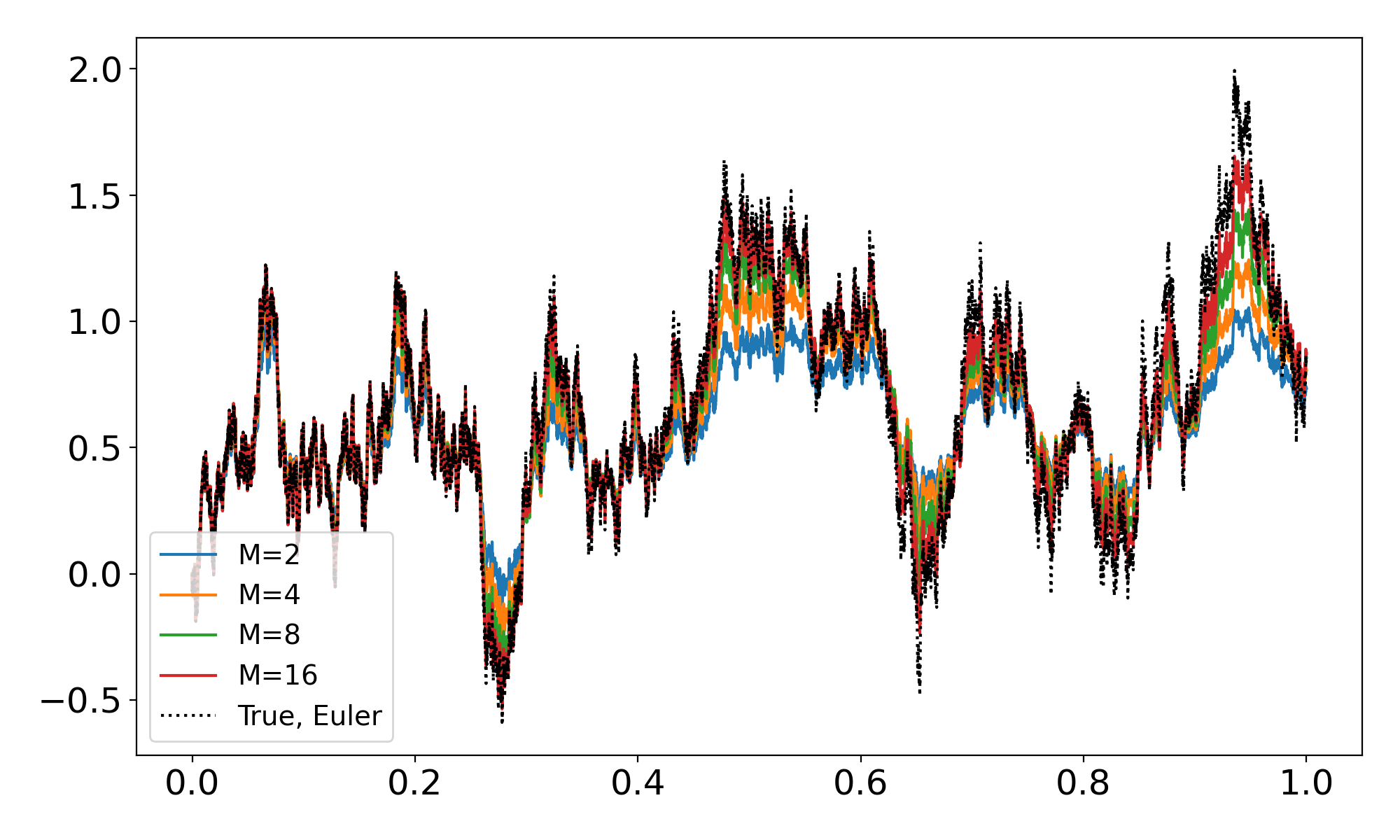
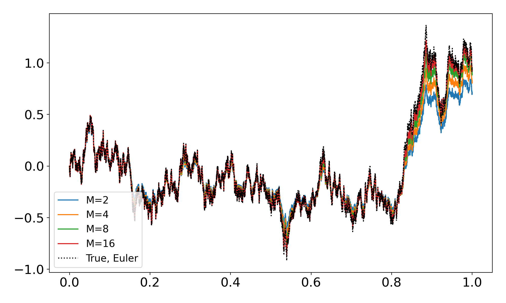
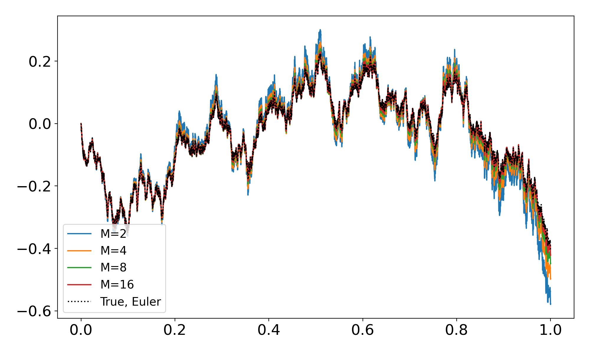
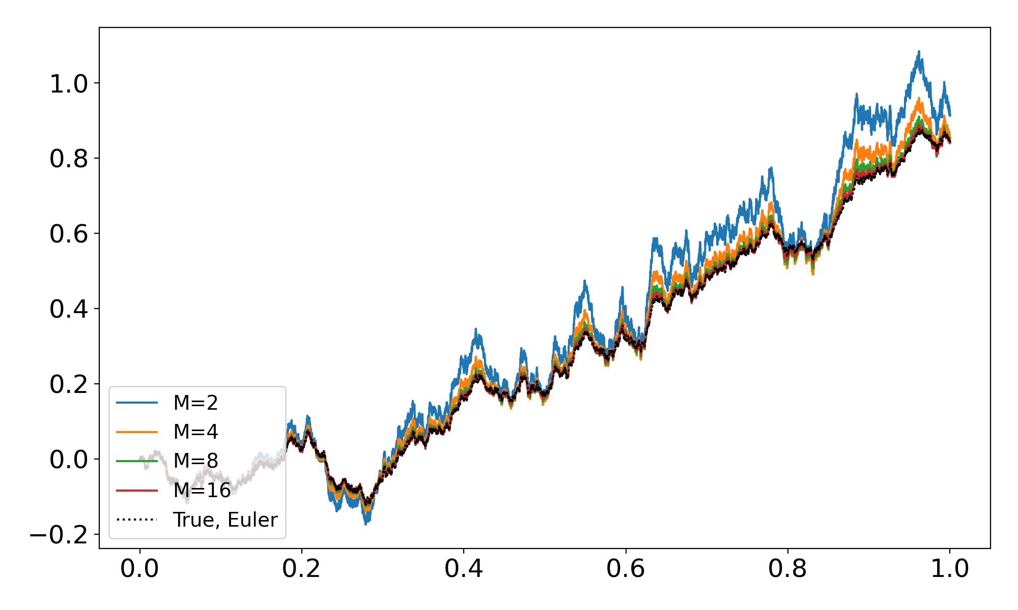
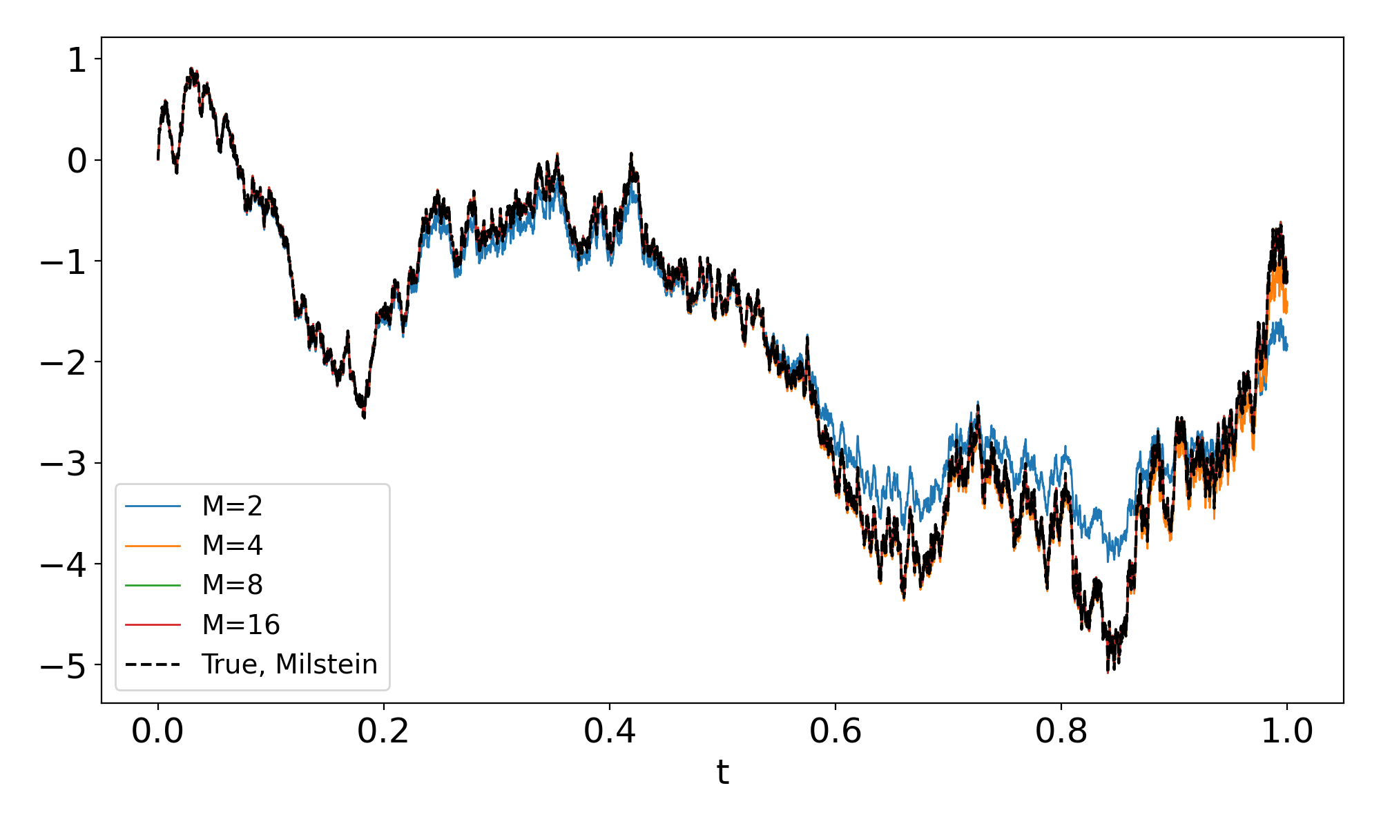
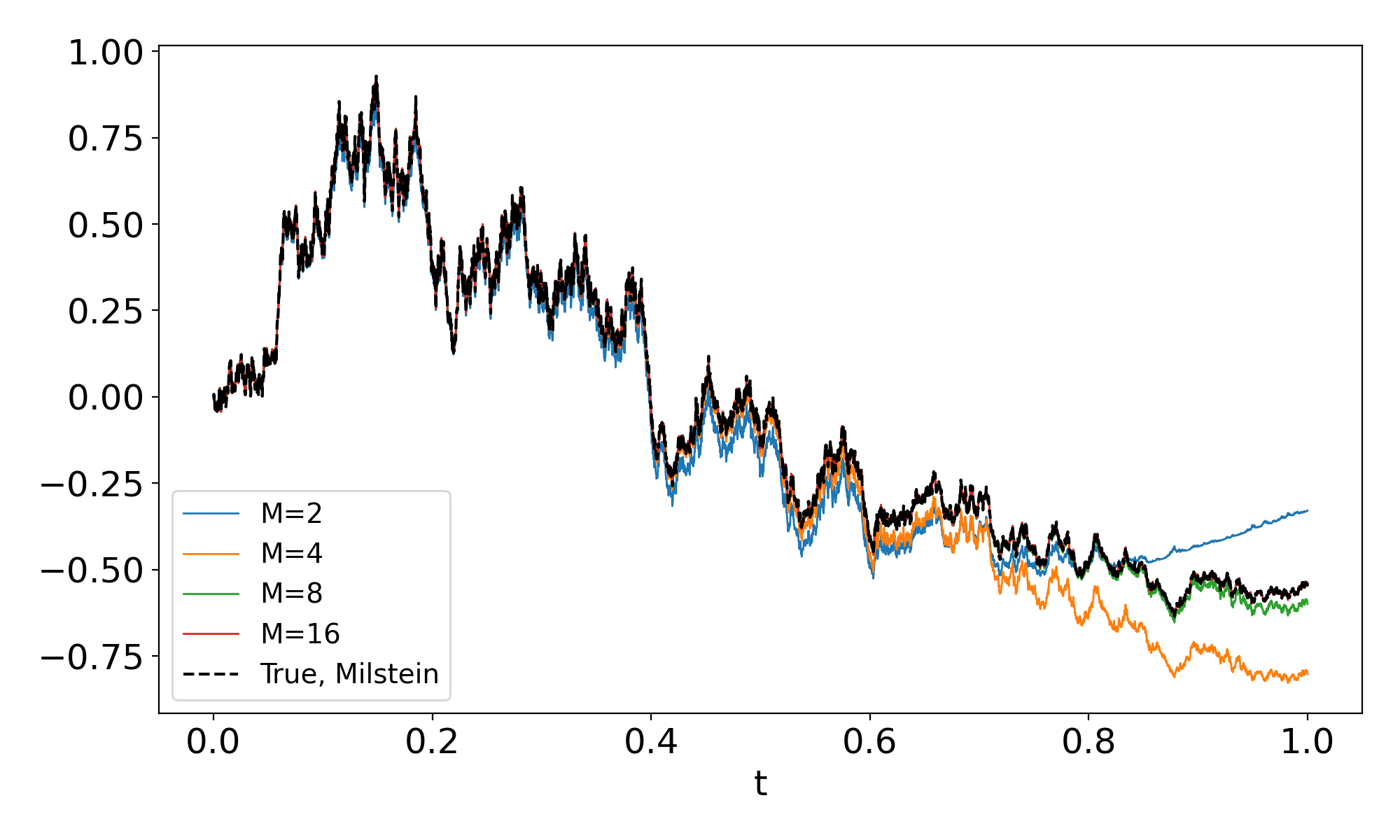
t\mapsto\left\langle\bm{\ell},\widehat{\mathbb{W}}_{t}\right\rangle is continuous and the strong error of convergence of the truncated linear combination of the signature elements satisfies
𝔼 [ sup t ∈ [ 0 , T ] | ⟨ ℓ , 𝕎 ^ t ≤ M ⟩ − ⟨ ℓ , 𝕎 ^ t ⟩ | ] ≤ ∑ n = M ∞ ∑ \mathcolor N a v y B l u e 𝐯 ∈ V n | ℓ \mathcolor N a v y B l u e 𝐯 | h T ( \mathcolor N a v y B l u e 𝐯 ) , M ∈ ℕ . formulae-sequence 𝔼 delimited-[] subscript supremum 𝑡 0 𝑇 bold-ℓ superscript subscript ^ 𝕎 𝑡 absent 𝑀
bold-ℓ subscript ^ 𝕎 𝑡
superscript subscript 𝑛 𝑀 subscript \mathcolor 𝑁 𝑎 𝑣 𝑦 𝐵 𝑙 𝑢 𝑒 𝐯 subscript 𝑉 𝑛 superscript bold-ℓ \mathcolor 𝑁 𝑎 𝑣 𝑦 𝐵 𝑙 𝑢 𝑒 𝐯 subscript ℎ 𝑇 \mathcolor 𝑁 𝑎 𝑣 𝑦 𝐵 𝑙 𝑢 𝑒 𝐯 𝑀 ℕ \displaystyle\mathbb{E}\left[\sup_{t\in[0,T]}\left|\left\langle\bm{\ell},\widehat{\mathbb{W}}_{t}^{\leq M}\right\rangle-\left\langle\bm{\ell},\widehat{\mathbb{W}}_{t}\right\rangle\right|\right]\leq\sum_{n=M}^{\infty}\sum_{{\mathcolor{NavyBlue}{\mathbf{v}}}\in V_{n}}\left|\bm{\ell}^{\mathcolor{NavyBlue}{\mathbf{v}}}\right|h_{T}({\mathcolor{NavyBlue}{\mathbf{v}}}),\quad M\in\mathbb{N}. (3.21)
Proof.
(i )
For all ℓ ∈ 𝒜 h bold-ℓ subscript 𝒜 ℎ \bm{\ell}\in{\mathcal{A}_{h}} 3.18
𝔼 [ sup s ∈ [ 0 , t ] ‖ ℓ ‖ s 𝒜 ] ≤ ∑ n = 0 ∞ ∑ \mathcolor N a v y B l u e 𝐯 ∈ V n | ℓ \mathcolor N a v y B l u e 𝐯 | 𝔼 [ sup s ∈ [ 0 , t ] | ⟨ \mathcolor N a v y B l u e 𝐯 , 𝕎 ^ s ⟩ | ] ≤ ∑ n = 0 ∞ ∑ \mathcolor N a v y B l u e 𝐯 ∈ V n | ℓ \mathcolor N a v y B l u e 𝐯 | h t ( \mathcolor N a v y B l u e 𝐯 ) ≤ ‖ ℓ ‖ t 𝒜 h < ∞ . 𝔼 delimited-[] subscript supremum 𝑠 0 𝑡 superscript subscript norm bold-ℓ 𝑠 𝒜 superscript subscript 𝑛 0 subscript \mathcolor 𝑁 𝑎 𝑣 𝑦 𝐵 𝑙 𝑢 𝑒 𝐯 subscript 𝑉 𝑛 superscript bold-ℓ \mathcolor 𝑁 𝑎 𝑣 𝑦 𝐵 𝑙 𝑢 𝑒 𝐯 𝔼 delimited-[] subscript supremum 𝑠 0 𝑡 \mathcolor 𝑁 𝑎 𝑣 𝑦 𝐵 𝑙 𝑢 𝑒 𝐯 subscript ^ 𝕎 𝑠
superscript subscript 𝑛 0 subscript \mathcolor 𝑁 𝑎 𝑣 𝑦 𝐵 𝑙 𝑢 𝑒 𝐯 subscript 𝑉 𝑛 superscript bold-ℓ \mathcolor 𝑁 𝑎 𝑣 𝑦 𝐵 𝑙 𝑢 𝑒 𝐯 subscript ℎ 𝑡 \mathcolor 𝑁 𝑎 𝑣 𝑦 𝐵 𝑙 𝑢 𝑒 𝐯 superscript subscript norm bold-ℓ 𝑡 subscript 𝒜 ℎ \displaystyle\mathbb{E}\left[\sup_{s\in[0,t]}\left|\left|\bm{\ell}\right|\right|_{s}^{\mathcal{A}}\right]\leq\sum_{n=0}^{\infty}\sum_{{\mathcolor{NavyBlue}{\mathbf{v}}}\in V_{n}}\left|\bm{\ell}^{\mathcolor{NavyBlue}{\mathbf{v}}}\right|\mathbb{E}\left[\sup_{s\in[0,t]}\left|\left\langle{\mathcolor{NavyBlue}{\mathbf{v}}},\widehat{\mathbb{W}}_{s}\right\rangle\right|\right]\leq\sum_{n=0}^{\infty}\sum_{{\mathcolor{NavyBlue}{\mathbf{v}}}\in V_{n}}\left|\bm{\ell}^{\mathcolor{NavyBlue}{\mathbf{v}}}\right|h_{t}({\mathcolor{NavyBlue}{\mathbf{v}}})\leq\left|\left|\bm{\ell}\right|\right|_{t}^{\mathcal{A}_{h}}<\infty. (3.22)
Consequently, sup t ∈ [ 0 , T ] ‖ ℓ ‖ t 𝒜 < ∞ a.s. subscript supremum 𝑡 0 𝑇 superscript subscript norm bold-ℓ 𝑡 𝒜 a.s. \sup_{t\in[0,T]}\left|\left|\bm{\ell}\right|\right|_{t}^{\mathcal{A}}<\infty\text{ a.s.} ℓ ∈ 𝒜 ( 𝕎 ^ ) bold-ℓ 𝒜 ^ 𝕎 \bm{\ell}\in\mathcal{A}(\widehat{\mathbb{W}})
(ii )
Starting with
⟨ ℓ , 𝕎 ^ s ⟩ 2 superscript bold-ℓ subscript ^ 𝕎 𝑠
2 \displaystyle\left\langle\bm{\ell},\widehat{\mathbb{W}}_{s}\right\rangle^{2} = ( ∑ \mathcolor N a v y B l u e 𝐯 ∈ V ℓ \mathcolor N a v y B l u e 𝐯 ⟨ \mathcolor N a v y B l u e 𝐯 , 𝕎 ^ s ⟩ ) 2 ≤ ∑ \mathcolor N a v y B l u e 𝐮 ∈ V ∑ \mathcolor N a v y B l u e 𝐰 ∈ V | ℓ \mathcolor N a v y B l u e 𝐮 ℓ \mathcolor N a v y B l u e 𝐰 | ⋅ | ⟨ \mathcolor N a v y B l u e 𝐮 , 𝕎 ^ s ⟩ ⟨ \mathcolor N a v y B l u e 𝐰 , 𝕎 ^ s ⟩ | , absent superscript subscript \mathcolor 𝑁 𝑎 𝑣 𝑦 𝐵 𝑙 𝑢 𝑒 𝐯 𝑉 superscript bold-ℓ \mathcolor 𝑁 𝑎 𝑣 𝑦 𝐵 𝑙 𝑢 𝑒 𝐯 \mathcolor 𝑁 𝑎 𝑣 𝑦 𝐵 𝑙 𝑢 𝑒 𝐯 subscript ^ 𝕎 𝑠
2 subscript \mathcolor 𝑁 𝑎 𝑣 𝑦 𝐵 𝑙 𝑢 𝑒 𝐮 𝑉 subscript \mathcolor 𝑁 𝑎 𝑣 𝑦 𝐵 𝑙 𝑢 𝑒 𝐰 𝑉 ⋅ superscript bold-ℓ \mathcolor 𝑁 𝑎 𝑣 𝑦 𝐵 𝑙 𝑢 𝑒 𝐮 superscript bold-ℓ \mathcolor 𝑁 𝑎 𝑣 𝑦 𝐵 𝑙 𝑢 𝑒 𝐰 \mathcolor 𝑁 𝑎 𝑣 𝑦 𝐵 𝑙 𝑢 𝑒 𝐮 subscript ^ 𝕎 𝑠
\mathcolor 𝑁 𝑎 𝑣 𝑦 𝐵 𝑙 𝑢 𝑒 𝐰 subscript ^ 𝕎 𝑠
\displaystyle=\left(\sum_{{\mathcolor{NavyBlue}{\mathbf{v}}}\in V}\bm{\ell}^{\mathcolor{NavyBlue}{\mathbf{v}}}\left\langle{\mathcolor{NavyBlue}{\mathbf{v}}},\widehat{\mathbb{W}}_{s}\right\rangle\right)^{2}\leq\sum_{{\mathcolor{NavyBlue}{\mathbf{u}}}\in V}\sum_{{\mathcolor{NavyBlue}{\mathbf{w}}}\in V}\left|\bm{\ell}^{\mathcolor{NavyBlue}{\mathbf{u}}}\bm{\ell}^{\mathcolor{NavyBlue}{\mathbf{w}}}\right|\cdot\left|\left\langle{\mathcolor{NavyBlue}{\mathbf{u}}},\widehat{\mathbb{W}}_{s}\right\rangle\left\langle{\mathcolor{NavyBlue}{\mathbf{w}}},\widehat{\mathbb{W}}_{s}\right\rangle\right|,
we get that
sup s ∈ [ 0 , t ] ⟨ ℓ , 𝕎 ^ s ⟩ 2 ≤ ∑ \mathcolor N a v y B l u e 𝐮 ∈ V ∑ \mathcolor N a v y B l u e 𝐰 ∈ V | ℓ \mathcolor N a v y B l u e 𝐮 ℓ \mathcolor N a v y B l u e 𝐰 | ⋅ sup s ∈ [ 0 , t ] | ⟨ \mathcolor N a v y B l u e 𝐮 , 𝕎 ^ s ⟩ | ⋅ sup s ∈ [ 0 , t ] | ⟨ \mathcolor N a v y B l u e 𝐰 , 𝕎 ^ s ⟩ | . subscript supremum 𝑠 0 𝑡 superscript bold-ℓ subscript ^ 𝕎 𝑠
2 subscript \mathcolor 𝑁 𝑎 𝑣 𝑦 𝐵 𝑙 𝑢 𝑒 𝐮 𝑉 subscript \mathcolor 𝑁 𝑎 𝑣 𝑦 𝐵 𝑙 𝑢 𝑒 𝐰 𝑉 ⋅ superscript bold-ℓ \mathcolor 𝑁 𝑎 𝑣 𝑦 𝐵 𝑙 𝑢 𝑒 𝐮 superscript bold-ℓ \mathcolor 𝑁 𝑎 𝑣 𝑦 𝐵 𝑙 𝑢 𝑒 𝐰 subscript supremum 𝑠 0 𝑡 ⋅ \mathcolor 𝑁 𝑎 𝑣 𝑦 𝐵 𝑙 𝑢 𝑒 𝐮 subscript ^ 𝕎 𝑠
subscript supremum 𝑠 0 𝑡 \mathcolor 𝑁 𝑎 𝑣 𝑦 𝐵 𝑙 𝑢 𝑒 𝐰 subscript ^ 𝕎 𝑠
\sup_{s\in[0,t]}\left\langle\bm{\ell},\widehat{\mathbb{W}}_{s}\right\rangle^{2}\leq\sum_{{\mathcolor{NavyBlue}{\mathbf{u}}}\in V}\sum_{{\mathcolor{NavyBlue}{\mathbf{w}}}\in V}\left|\bm{\ell}^{\mathcolor{NavyBlue}{\mathbf{u}}}\bm{\ell}^{\mathcolor{NavyBlue}{\mathbf{w}}}\right|\cdot\sup_{s\in[0,t]}\left|\left\langle{\mathcolor{NavyBlue}{\mathbf{u}}},\widehat{\mathbb{W}}_{s}\right\rangle\right|\cdot\sup_{s\in[0,t]}\left|\left\langle{\mathcolor{NavyBlue}{\mathbf{w}}},\widehat{\mathbb{W}}_{s}\right\rangle\right|.
Taking the expectation and applying Cauchy-Schwarz inequality yields that
𝔼 [ sup s ∈ [ 0 , t ] ⟨ ℓ , 𝕎 ^ s ⟩ 2 ] 𝔼 delimited-[] subscript supremum 𝑠 0 𝑡 superscript bold-ℓ subscript ^ 𝕎 𝑠
2 \displaystyle\mathbb{E}\left[\sup_{s\in[0,t]}\left\langle\bm{\ell},\widehat{\mathbb{W}}_{s}\right\rangle^{2}\right] ≤ ∑ \mathcolor N a v y B l u e 𝐮 ∈ V ∑ \mathcolor N a v y B l u e 𝐰 ∈ V | ℓ \mathcolor N a v y B l u e 𝐮 ℓ \mathcolor N a v y B l u e 𝐰 | 𝔼 sup s ∈ [ 0 , t ] ⟨ \mathcolor N a v y B l u e 𝐮 , 𝕎 ^ s ⟩ 2 𝔼 sup s ∈ [ 0 , t ] ⟨ \mathcolor N a v y B l u e 𝐰 , 𝕎 ^ s ⟩ 2 absent subscript \mathcolor 𝑁 𝑎 𝑣 𝑦 𝐵 𝑙 𝑢 𝑒 𝐮 𝑉 subscript \mathcolor 𝑁 𝑎 𝑣 𝑦 𝐵 𝑙 𝑢 𝑒 𝐰 𝑉 superscript bold-ℓ \mathcolor 𝑁 𝑎 𝑣 𝑦 𝐵 𝑙 𝑢 𝑒 𝐮 superscript bold-ℓ \mathcolor 𝑁 𝑎 𝑣 𝑦 𝐵 𝑙 𝑢 𝑒 𝐰 𝔼 subscript supremum 𝑠 0 𝑡 superscript \mathcolor 𝑁 𝑎 𝑣 𝑦 𝐵 𝑙 𝑢 𝑒 𝐮 subscript ^ 𝕎 𝑠
2 𝔼 subscript supremum 𝑠 0 𝑡 superscript \mathcolor 𝑁 𝑎 𝑣 𝑦 𝐵 𝑙 𝑢 𝑒 𝐰 subscript ^ 𝕎 𝑠
2 \displaystyle\leq\sum_{{\mathcolor{NavyBlue}{\mathbf{u}}}\in V}\sum_{{\mathcolor{NavyBlue}{\mathbf{w}}}\in V}\left|\bm{\ell}^{\mathcolor{NavyBlue}{\mathbf{u}}}\bm{\ell}^{\mathcolor{NavyBlue}{\mathbf{w}}}\right|\sqrt{\mathbb{E}\sup_{s\in[0,t]}\left\langle{\mathcolor{NavyBlue}{\mathbf{u}}},\widehat{\mathbb{W}}_{s}\right\rangle^{2}}\sqrt{\mathbb{E}\sup_{s\in[0,t]}\left\langle{\mathcolor{NavyBlue}{\mathbf{w}}},\widehat{\mathbb{W}}_{s}\right\rangle^{2}}
= ( ∑ \mathcolor N a v y B l u e 𝐯 ∈ V | ℓ \mathcolor N a v y B l u e 𝐯 | 𝔼 sup s ∈ [ 0 , t ] ⟨ \mathcolor N a v y B l u e 𝐯 , 𝕎 ^ s ⟩ 2 ) 2 absent superscript subscript \mathcolor 𝑁 𝑎 𝑣 𝑦 𝐵 𝑙 𝑢 𝑒 𝐯 𝑉 superscript bold-ℓ \mathcolor 𝑁 𝑎 𝑣 𝑦 𝐵 𝑙 𝑢 𝑒 𝐯 𝔼 subscript supremum 𝑠 0 𝑡 superscript \mathcolor 𝑁 𝑎 𝑣 𝑦 𝐵 𝑙 𝑢 𝑒 𝐯 subscript ^ 𝕎 𝑠
2 2 \displaystyle=\left(\sum_{{\mathcolor{NavyBlue}{\mathbf{v}}}\in V}\left|\bm{\ell}^{\mathcolor{NavyBlue}{\mathbf{v}}}\right|\sqrt{\mathbb{E}\sup_{s\in[0,t]}\left\langle{\mathcolor{NavyBlue}{\mathbf{v}}},\widehat{\mathbb{W}}_{s}\right\rangle^{2}}\right)^{2}
≤ ( ∑ \mathcolor N a v y B l u e 𝐯 ∈ V | ℓ \mathcolor N a v y B l u e 𝐯 | h t ( \mathcolor N a v y B l u e 𝐯 ) ) 2 absent superscript subscript \mathcolor 𝑁 𝑎 𝑣 𝑦 𝐵 𝑙 𝑢 𝑒 𝐯 𝑉 superscript bold-ℓ \mathcolor 𝑁 𝑎 𝑣 𝑦 𝐵 𝑙 𝑢 𝑒 𝐯 subscript ℎ 𝑡 \mathcolor 𝑁 𝑎 𝑣 𝑦 𝐵 𝑙 𝑢 𝑒 𝐯 2 \displaystyle\leq\left(\sum_{{\mathcolor{NavyBlue}{\mathbf{v}}}\in V}\left|\bm{\ell}^{\mathcolor{NavyBlue}{\mathbf{v}}}\right|h_{t}({\mathcolor{NavyBlue}{\mathbf{v}}})\right)^{2}
= ( ‖ ℓ ‖ t 𝒜 h ) 2 . absent superscript superscript subscript norm bold-ℓ 𝑡 subscript 𝒜 ℎ 2 \displaystyle=\left(\left|\left|\bm{\ell}\right|\right|_{t}^{\mathcal{A}_{h}}\right)^{2}.
(iii )
Define
X t := ⟨ ℓ , 𝕎 ^ t ⟩ = ∑ n = 0 ∞ ∑ \mathcolor N a v y B l u e 𝐯 ∈ V n ℓ \mathcolor N a v y B l u e 𝐯 𝕎 ^ t \mathcolor N a v y B l u e 𝐯 and X t M := ⟨ ℓ , 𝕎 ^ t ≤ M ⟩ = ∑ n = 0 M ∑ \mathcolor N a v y B l u e 𝐯 ∈ V n ℓ \mathcolor N a v y B l u e 𝐯 𝕎 ^ t \mathcolor N a v y B l u e 𝐯 . formulae-sequence assign subscript 𝑋 𝑡 bold-ℓ subscript ^ 𝕎 𝑡
superscript subscript 𝑛 0 subscript \mathcolor 𝑁 𝑎 𝑣 𝑦 𝐵 𝑙 𝑢 𝑒 𝐯 subscript 𝑉 𝑛 superscript bold-ℓ \mathcolor 𝑁 𝑎 𝑣 𝑦 𝐵 𝑙 𝑢 𝑒 𝐯 superscript subscript ^ 𝕎 𝑡 \mathcolor 𝑁 𝑎 𝑣 𝑦 𝐵 𝑙 𝑢 𝑒 𝐯 assign and superscript subscript 𝑋 𝑡 𝑀
bold-ℓ superscript subscript ^ 𝕎 𝑡 absent 𝑀
superscript subscript 𝑛 0 𝑀 subscript \mathcolor 𝑁 𝑎 𝑣 𝑦 𝐵 𝑙 𝑢 𝑒 𝐯 subscript 𝑉 𝑛 superscript bold-ℓ \mathcolor 𝑁 𝑎 𝑣 𝑦 𝐵 𝑙 𝑢 𝑒 𝐯 superscript subscript ^ 𝕎 𝑡 \mathcolor 𝑁 𝑎 𝑣 𝑦 𝐵 𝑙 𝑢 𝑒 𝐯 \displaystyle X_{t}:=\left\langle\bm{\ell},\widehat{\mathbb{W}}_{t}\right\rangle=\sum_{n=0}^{\infty}\sum_{{\mathcolor{NavyBlue}{\mathbf{v}}}\in V_{n}}\bm{\ell}^{\mathcolor{NavyBlue}{\mathbf{v}}}\widehat{\mathbb{W}}_{t}^{\mathcolor{NavyBlue}{\mathbf{v}}}\quad\text{and}\quad X_{t}^{M}:=\left\langle\bm{\ell},\widehat{\mathbb{W}}_{t}^{\leq M}\right\rangle=\sum_{n=0}^{M}\sum_{{\mathcolor{NavyBlue}{\mathbf{v}}}\in V_{n}}\bm{\ell}^{\mathcolor{NavyBlue}{\mathbf{v}}}\widehat{\mathbb{W}}_{t}^{\mathcolor{NavyBlue}{\mathbf{v}}}. (3.23)
It follows from inequality (3.18
𝔼 [ sup t ∈ [ 0 , T ] | X t − X t M | ] 𝔼 delimited-[] subscript supremum 𝑡 0 𝑇 subscript 𝑋 𝑡 superscript subscript 𝑋 𝑡 𝑀 \displaystyle\mathbb{E}\left[\sup_{t\in[0,T]}\left|X_{t}-X_{t}^{M}\right|\right] ≤ ∑ n = M + 1 ∞ ∑ \mathcolor N a v y B l u e 𝐯 ∈ V n | ℓ \mathcolor N a v y B l u e 𝐯 | 𝔼 [ sup t ∈ [ 0 , T ] ⟨ \mathcolor N a v y B l u e 𝐯 , 𝕎 ^ t ⟩ ] ≤ ∑ n = M + 1 ∞ ∑ \mathcolor N a v y B l u e 𝐯 ∈ V n | ℓ \mathcolor N a v y B l u e 𝐯 | h T ( \mathcolor N a v y B l u e 𝐯 ) . absent superscript subscript 𝑛 𝑀 1 subscript \mathcolor 𝑁 𝑎 𝑣 𝑦 𝐵 𝑙 𝑢 𝑒 𝐯 subscript 𝑉 𝑛 superscript bold-ℓ \mathcolor 𝑁 𝑎 𝑣 𝑦 𝐵 𝑙 𝑢 𝑒 𝐯 𝔼 delimited-[] subscript supremum 𝑡 0 𝑇 \mathcolor 𝑁 𝑎 𝑣 𝑦 𝐵 𝑙 𝑢 𝑒 𝐯 subscript ^ 𝕎 𝑡
superscript subscript 𝑛 𝑀 1 subscript \mathcolor 𝑁 𝑎 𝑣 𝑦 𝐵 𝑙 𝑢 𝑒 𝐯 subscript 𝑉 𝑛 superscript bold-ℓ \mathcolor 𝑁 𝑎 𝑣 𝑦 𝐵 𝑙 𝑢 𝑒 𝐯 subscript ℎ 𝑇 \mathcolor 𝑁 𝑎 𝑣 𝑦 𝐵 𝑙 𝑢 𝑒 𝐯 \displaystyle\leq\sum_{n=M+1}^{\infty}\sum_{{\mathcolor{NavyBlue}{\mathbf{v}}}\in V_{n}}\left|\bm{\ell}^{\mathcolor{NavyBlue}{\mathbf{v}}}\right|\mathbb{E}\left[\sup_{t\in[0,T]}\left\langle{\mathcolor{NavyBlue}{\mathbf{v}}},\widehat{\mathbb{W}}_{t}\right\rangle\right]\leq\sum_{n=M+1}^{\infty}\sum_{{\mathcolor{NavyBlue}{\mathbf{v}}}\in V_{n}}\left|\bm{\ell}^{\mathcolor{NavyBlue}{\mathbf{v}}}\right|h_{T}({\mathcolor{NavyBlue}{\mathbf{v}}}). (3.24)
Moreover, ℓ ∈ 𝒜 h bold-ℓ subscript 𝒜 ℎ \bm{\ell}\in{\mathcal{A}_{h}}
lim M → ∞ ∑ n = M + 1 ∞ ∑ \mathcolor N a v y B l u e 𝐯 ∈ V n | ℓ \mathcolor N a v y B l u e 𝐯 | h T ( \mathcolor N a v y B l u e 𝐯 ) = 0 . subscript → 𝑀 superscript subscript 𝑛 𝑀 1 subscript \mathcolor 𝑁 𝑎 𝑣 𝑦 𝐵 𝑙 𝑢 𝑒 𝐯 subscript 𝑉 𝑛 superscript bold-ℓ \mathcolor 𝑁 𝑎 𝑣 𝑦 𝐵 𝑙 𝑢 𝑒 𝐯 subscript ℎ 𝑇 \mathcolor 𝑁 𝑎 𝑣 𝑦 𝐵 𝑙 𝑢 𝑒 𝐯 0 \lim_{M\to\infty}\sum_{n=M+1}^{\infty}\sum_{{\mathcolor{NavyBlue}{\mathbf{v}}}\in V_{n}}\left|\bm{\ell}^{\mathcolor{NavyBlue}{\mathbf{v}}}\right|h_{T}({\mathcolor{NavyBlue}{\mathbf{v}}})=0.
Thus
𝔼 [ sup t ∈ [ 0 , T ] | X t − X t M | ] → 0 , → 𝔼 delimited-[] subscript supremum 𝑡 0 𝑇 subscript 𝑋 𝑡 superscript subscript 𝑋 𝑡 𝑀 0 \mathbb{E}\left[\sup_{t\in[0,T]}\left|X_{t}-X_{t}^{M}\right|\right]\to 0, (3.25)
implying that
sup t ∈ [ 0 , T ] | X t − X t M | → 0 in probability as M → ∞ . → subscript supremum 𝑡 0 𝑇 subscript 𝑋 𝑡 superscript subscript 𝑋 𝑡 𝑀 0 in probability as M → ∞ .
\sup_{t\in[0,T]}\left|X_{t}-X_{t}^{M}\right|\to 0\quad\text{in probability as $M\to\infty$.}
So there exists a sub-sequence ( M k ) k ∈ ℕ subscript subscript 𝑀 𝑘 𝑘 ℕ (M_{k})_{k\in\mathbb{N}} sup t ∈ [ 0 , T ] | X t − X t M k | → 0 → subscript supremum 𝑡 0 𝑇 subscript 𝑋 𝑡 superscript subscript 𝑋 𝑡 subscript 𝑀 𝑘 0 \sup_{t\in[0,T]}\left|X_{t}-X_{t}^{M_{k}}\right|\to 0 X M k superscript 𝑋 subscript 𝑀 𝑘 X^{M_{k}} X 𝑋 X
∎
Derived from (3.17 | | ⋅ | | 𝒜 h \left|\left|\cdot\right|\right|^{\mathcal{A}_{h}}
Proposition 3.7 .
For every 𝐩 , ℓ ∈ T ( ( ℝ d ) ) 𝐩 bold-ℓ
𝑇 superscript ℝ 𝑑 \bm{p},\bm{\ell}\in T((\mathbb{R}^{d}))
‖ 𝒑 ℓ ‖ t 𝒜 h ≤ ‖ 𝒑 ‖ t 𝒜 h ‖ ℓ ‖ t 𝒜 h . superscript subscript norm 𝒑 bold-ℓ 𝑡 subscript 𝒜 ℎ superscript subscript norm 𝒑 𝑡 subscript 𝒜 ℎ superscript subscript norm bold-ℓ 𝑡 subscript 𝒜 ℎ \left|\left|\bm{p}\bm{\ell}\right|\right|_{t}^{\mathcal{A}_{h}}\leq\left|\left|\bm{p}\right|\right|_{t}^{\mathcal{A}_{h}}\left|\left|\bm{\ell}\right|\right|_{t}^{\mathcal{A}_{h}}.
In particular, if 𝐩 , ℓ ∈ 𝒜 h 𝐩 bold-ℓ
subscript 𝒜 ℎ \bm{p},\bm{\ell}\in{\mathcal{A}_{h}} 𝐩 ℓ ∈ 𝒜 h 𝐩 bold-ℓ subscript 𝒜 ℎ \bm{p}\bm{\ell}\in{\mathcal{A}_{h}}
Proof.
First notice that for all k ∈ ℕ 𝑘 ℕ k\in\mathbb{N} \mathcolor N a v y B l u e 𝐰 ∈ V k \mathcolor 𝑁 𝑎 𝑣 𝑦 𝐵 𝑙 𝑢 𝑒 𝐰 subscript 𝑉 𝑘 {\mathcolor{NavyBlue}{\mathbf{w}}}\in V_{k}
⟨ 𝒑 ℓ , \mathcolor N a v y B l u e 𝐰 ⟩ = ∑ n = 0 k ∑ \mathcolor N a v y B l u e 𝐮 ∈ V n ∑ \mathcolor N a v y B l u e 𝐯 ∈ V k − n 𝒑 \mathcolor N a v y B l u e 𝐮 ℓ \mathcolor N a v y B l u e 𝐯 ⟨ \mathcolor N a v y B l u e 𝐮 \mathcolor N a v y B l u e 𝐯 , \mathcolor N a v y B l u e 𝐰 ⟩ , 𝒑 bold-ℓ \mathcolor 𝑁 𝑎 𝑣 𝑦 𝐵 𝑙 𝑢 𝑒 𝐰
superscript subscript 𝑛 0 𝑘 subscript \mathcolor 𝑁 𝑎 𝑣 𝑦 𝐵 𝑙 𝑢 𝑒 𝐮 subscript 𝑉 𝑛 subscript \mathcolor 𝑁 𝑎 𝑣 𝑦 𝐵 𝑙 𝑢 𝑒 𝐯 subscript 𝑉 𝑘 𝑛 superscript 𝒑 \mathcolor 𝑁 𝑎 𝑣 𝑦 𝐵 𝑙 𝑢 𝑒 𝐮 superscript bold-ℓ \mathcolor 𝑁 𝑎 𝑣 𝑦 𝐵 𝑙 𝑢 𝑒 𝐯 \mathcolor 𝑁 𝑎 𝑣 𝑦 𝐵 𝑙 𝑢 𝑒 𝐮 \mathcolor 𝑁 𝑎 𝑣 𝑦 𝐵 𝑙 𝑢 𝑒 𝐯 \mathcolor 𝑁 𝑎 𝑣 𝑦 𝐵 𝑙 𝑢 𝑒 𝐰
\left\langle\bm{p}\bm{\ell},{\mathcolor{NavyBlue}{\mathbf{w}}}\right\rangle=\sum_{n=0}^{k}\sum_{{\mathcolor{NavyBlue}{\mathbf{u}}}\in V_{n}}\sum_{{\mathcolor{NavyBlue}{\mathbf{v}}}\in V_{k-n}}\bm{p}^{\mathcolor{NavyBlue}{\mathbf{u}}}\bm{\ell}^{\mathcolor{NavyBlue}{\mathbf{v}}}\left\langle{\mathcolor{NavyBlue}{\mathbf{u}}}{\mathcolor{NavyBlue}{\mathbf{v}}},{\mathcolor{NavyBlue}{\mathbf{w}}}\right\rangle,
so that
‖ 𝒑 ℓ ‖ t 𝒜 h superscript subscript norm 𝒑 bold-ℓ 𝑡 subscript 𝒜 ℎ \displaystyle\left|\left|\bm{p}\bm{\ell}\right|\right|_{t}^{\mathcal{A}_{h}} = ∑ k = 0 ∞ ∑ \mathcolor N a v y B l u e 𝐰 ∈ V k | ⟨ 𝒑 ℓ , \mathcolor N a v y B l u e 𝐰 ⟩ | h t ( \mathcolor N a v y B l u e 𝐰 ) absent superscript subscript 𝑘 0 subscript \mathcolor 𝑁 𝑎 𝑣 𝑦 𝐵 𝑙 𝑢 𝑒 𝐰 subscript 𝑉 𝑘 𝒑 bold-ℓ \mathcolor 𝑁 𝑎 𝑣 𝑦 𝐵 𝑙 𝑢 𝑒 𝐰
subscript ℎ 𝑡 \mathcolor 𝑁 𝑎 𝑣 𝑦 𝐵 𝑙 𝑢 𝑒 𝐰 \displaystyle=\sum_{k=0}^{\infty}\sum_{{\mathcolor{NavyBlue}{\mathbf{w}}}\in V_{k}}\left|\left\langle\bm{p}\bm{\ell},{\mathcolor{NavyBlue}{\mathbf{w}}}\right\rangle\right|h_{t}({\mathcolor{NavyBlue}{\mathbf{w}}}) (3.26)
= ∑ k = 0 ∞ ∑ \mathcolor N a v y B l u e 𝐰 ∈ V k | ∑ n = 0 k ∑ \mathcolor N a v y B l u e 𝐮 ∈ V n ∑ \mathcolor N a v y B l u e 𝐯 ∈ V k − n 𝒑 \mathcolor N a v y B l u e 𝐮 ℓ \mathcolor N a v y B l u e 𝐯 ⟨ \mathcolor N a v y B l u e 𝐮 \mathcolor N a v y B l u e 𝐯 , \mathcolor N a v y B l u e 𝐰 ⟩ | h t ( \mathcolor N a v y B l u e 𝐰 ) absent superscript subscript 𝑘 0 subscript \mathcolor 𝑁 𝑎 𝑣 𝑦 𝐵 𝑙 𝑢 𝑒 𝐰 subscript 𝑉 𝑘 superscript subscript 𝑛 0 𝑘 subscript \mathcolor 𝑁 𝑎 𝑣 𝑦 𝐵 𝑙 𝑢 𝑒 𝐮 subscript 𝑉 𝑛 subscript \mathcolor 𝑁 𝑎 𝑣 𝑦 𝐵 𝑙 𝑢 𝑒 𝐯 subscript 𝑉 𝑘 𝑛 superscript 𝒑 \mathcolor 𝑁 𝑎 𝑣 𝑦 𝐵 𝑙 𝑢 𝑒 𝐮 superscript bold-ℓ \mathcolor 𝑁 𝑎 𝑣 𝑦 𝐵 𝑙 𝑢 𝑒 𝐯 \mathcolor 𝑁 𝑎 𝑣 𝑦 𝐵 𝑙 𝑢 𝑒 𝐮 \mathcolor 𝑁 𝑎 𝑣 𝑦 𝐵 𝑙 𝑢 𝑒 𝐯 \mathcolor 𝑁 𝑎 𝑣 𝑦 𝐵 𝑙 𝑢 𝑒 𝐰
subscript ℎ 𝑡 \mathcolor 𝑁 𝑎 𝑣 𝑦 𝐵 𝑙 𝑢 𝑒 𝐰 \displaystyle=\sum_{k=0}^{\infty}\sum_{{\mathcolor{NavyBlue}{\mathbf{w}}}\in V_{k}}\left|\sum_{n=0}^{k}\sum_{{\mathcolor{NavyBlue}{\mathbf{u}}}\in V_{n}}\sum_{{\mathcolor{NavyBlue}{\mathbf{v}}}\in V_{k-n}}\bm{p}^{\mathcolor{NavyBlue}{\mathbf{u}}}\bm{\ell}^{\mathcolor{NavyBlue}{\mathbf{v}}}\left\langle{\mathcolor{NavyBlue}{\mathbf{u}}}{\mathcolor{NavyBlue}{\mathbf{v}}},{\mathcolor{NavyBlue}{\mathbf{w}}}\right\rangle\right|h_{t}({\mathcolor{NavyBlue}{\mathbf{w}}}) (3.27)
≤ ∑ k = 0 ∞ ∑ n = 0 k ∑ \mathcolor N a v y B l u e 𝐮 ∈ V n ∑ \mathcolor N a v y B l u e 𝐯 ∈ V k − n ∑ \mathcolor N a v y B l u e 𝐰 ∈ V k | 𝒑 \mathcolor N a v y B l u e 𝐮 ℓ \mathcolor N a v y B l u e 𝐯 | ⟨ \mathcolor N a v y B l u e 𝐮 \mathcolor N a v y B l u e 𝐯 , \mathcolor N a v y B l u e 𝐰 ⟩ h t ( \mathcolor N a v y B l u e 𝐰 ) absent superscript subscript 𝑘 0 superscript subscript 𝑛 0 𝑘 subscript \mathcolor 𝑁 𝑎 𝑣 𝑦 𝐵 𝑙 𝑢 𝑒 𝐮 subscript 𝑉 𝑛 subscript \mathcolor 𝑁 𝑎 𝑣 𝑦 𝐵 𝑙 𝑢 𝑒 𝐯 subscript 𝑉 𝑘 𝑛 subscript \mathcolor 𝑁 𝑎 𝑣 𝑦 𝐵 𝑙 𝑢 𝑒 𝐰 subscript 𝑉 𝑘 superscript 𝒑 \mathcolor 𝑁 𝑎 𝑣 𝑦 𝐵 𝑙 𝑢 𝑒 𝐮 superscript bold-ℓ \mathcolor 𝑁 𝑎 𝑣 𝑦 𝐵 𝑙 𝑢 𝑒 𝐯 \mathcolor 𝑁 𝑎 𝑣 𝑦 𝐵 𝑙 𝑢 𝑒 𝐮 \mathcolor 𝑁 𝑎 𝑣 𝑦 𝐵 𝑙 𝑢 𝑒 𝐯 \mathcolor 𝑁 𝑎 𝑣 𝑦 𝐵 𝑙 𝑢 𝑒 𝐰
subscript ℎ 𝑡 \mathcolor 𝑁 𝑎 𝑣 𝑦 𝐵 𝑙 𝑢 𝑒 𝐰 \displaystyle\leq\sum_{k=0}^{\infty}\sum_{n=0}^{k}\sum_{{\mathcolor{NavyBlue}{\mathbf{u}}}\in V_{n}}\sum_{{\mathcolor{NavyBlue}{\mathbf{v}}}\in V_{k-n}}\sum_{{\mathcolor{NavyBlue}{\mathbf{w}}}\in V_{k}}\left|\bm{p}^{\mathcolor{NavyBlue}{\mathbf{u}}}\bm{\ell}^{\mathcolor{NavyBlue}{\mathbf{v}}}\right|\left\langle{\mathcolor{NavyBlue}{\mathbf{u}}}{\mathcolor{NavyBlue}{\mathbf{v}}},{\mathcolor{NavyBlue}{\mathbf{w}}}\right\rangle h_{t}({\mathcolor{NavyBlue}{\mathbf{w}}}) (3.28)
Then, using (3.17
‖ 𝒑 ℓ ‖ t 𝒜 h superscript subscript norm 𝒑 bold-ℓ 𝑡 subscript 𝒜 ℎ \displaystyle\left|\left|\bm{p}\bm{\ell}\right|\right|_{t}^{\mathcal{A}_{h}} ≤ ∑ k = 0 ∞ ∑ n = 0 k ∑ \mathcolor N a v y B l u e 𝐮 ∈ V n ∑ \mathcolor N a v y B l u e 𝐯 ∈ V k − n | 𝒑 \mathcolor N a v y B l u e 𝐮 ℓ \mathcolor N a v y B l u e 𝐯 | h t ( \mathcolor N a v y B l u e 𝐮 ) h t ( \mathcolor N a v y B l u e 𝐯 ) ∑ \mathcolor N a v y B l u e 𝐰 ∈ V k ⟨ \mathcolor N a v y B l u e 𝐮 \mathcolor N a v y B l u e 𝐯 , \mathcolor N a v y B l u e 𝐰 ⟩ absent superscript subscript 𝑘 0 superscript subscript 𝑛 0 𝑘 subscript \mathcolor 𝑁 𝑎 𝑣 𝑦 𝐵 𝑙 𝑢 𝑒 𝐮 subscript 𝑉 𝑛 subscript \mathcolor 𝑁 𝑎 𝑣 𝑦 𝐵 𝑙 𝑢 𝑒 𝐯 subscript 𝑉 𝑘 𝑛 superscript 𝒑 \mathcolor 𝑁 𝑎 𝑣 𝑦 𝐵 𝑙 𝑢 𝑒 𝐮 superscript bold-ℓ \mathcolor 𝑁 𝑎 𝑣 𝑦 𝐵 𝑙 𝑢 𝑒 𝐯 subscript ℎ 𝑡 \mathcolor 𝑁 𝑎 𝑣 𝑦 𝐵 𝑙 𝑢 𝑒 𝐮 subscript ℎ 𝑡 \mathcolor 𝑁 𝑎 𝑣 𝑦 𝐵 𝑙 𝑢 𝑒 𝐯 subscript \mathcolor 𝑁 𝑎 𝑣 𝑦 𝐵 𝑙 𝑢 𝑒 𝐰 subscript 𝑉 𝑘 \mathcolor 𝑁 𝑎 𝑣 𝑦 𝐵 𝑙 𝑢 𝑒 𝐮 \mathcolor 𝑁 𝑎 𝑣 𝑦 𝐵 𝑙 𝑢 𝑒 𝐯 \mathcolor 𝑁 𝑎 𝑣 𝑦 𝐵 𝑙 𝑢 𝑒 𝐰
\displaystyle\leq\sum_{k=0}^{\infty}\sum_{n=0}^{k}\sum_{{\mathcolor{NavyBlue}{\mathbf{u}}}\in V_{n}}\sum_{{\mathcolor{NavyBlue}{\mathbf{v}}}\in V_{k-n}}\left|\bm{p}^{\mathcolor{NavyBlue}{\mathbf{u}}}\bm{\ell}^{\mathcolor{NavyBlue}{\mathbf{v}}}\right|h_{t}({\mathcolor{NavyBlue}{\mathbf{u}}})h_{t}({\mathcolor{NavyBlue}{\mathbf{v}}})\sum_{{\mathcolor{NavyBlue}{\mathbf{w}}}\in V_{k}}\left\langle{\mathcolor{NavyBlue}{\mathbf{u}}}{\mathcolor{NavyBlue}{\mathbf{v}}},{\mathcolor{NavyBlue}{\mathbf{w}}}\right\rangle (3.29)
= ∑ m = 0 ∞ ∑ n = 0 ∞ ∑ \mathcolor N a v y B l u e 𝐮 ∈ V n ∑ \mathcolor N a v y B l u e 𝐯 ∈ V m | 𝒑 \mathcolor N a v y B l u e 𝐮 ℓ \mathcolor N a v y B l u e 𝐯 | h t ( \mathcolor N a v y B l u e 𝐮 ) h t ( \mathcolor N a v y B l u e 𝐯 ) absent superscript subscript 𝑚 0 superscript subscript 𝑛 0 subscript \mathcolor 𝑁 𝑎 𝑣 𝑦 𝐵 𝑙 𝑢 𝑒 𝐮 subscript 𝑉 𝑛 subscript \mathcolor 𝑁 𝑎 𝑣 𝑦 𝐵 𝑙 𝑢 𝑒 𝐯 subscript 𝑉 𝑚 superscript 𝒑 \mathcolor 𝑁 𝑎 𝑣 𝑦 𝐵 𝑙 𝑢 𝑒 𝐮 superscript bold-ℓ \mathcolor 𝑁 𝑎 𝑣 𝑦 𝐵 𝑙 𝑢 𝑒 𝐯 subscript ℎ 𝑡 \mathcolor 𝑁 𝑎 𝑣 𝑦 𝐵 𝑙 𝑢 𝑒 𝐮 subscript ℎ 𝑡 \mathcolor 𝑁 𝑎 𝑣 𝑦 𝐵 𝑙 𝑢 𝑒 𝐯 \displaystyle=\sum_{m=0}^{\infty}\sum_{n=0}^{\infty}\sum_{{\mathcolor{NavyBlue}{\mathbf{u}}}\in V_{n}}\sum_{{\mathcolor{NavyBlue}{\mathbf{v}}}\in V_{m}}\left|\bm{p}^{\mathcolor{NavyBlue}{\mathbf{u}}}\bm{\ell}^{\mathcolor{NavyBlue}{\mathbf{v}}}\right|h_{t}({\mathcolor{NavyBlue}{\mathbf{u}}})h_{t}({\mathcolor{NavyBlue}{\mathbf{v}}}) (3.30)
= ‖ 𝒑 ‖ t 𝒜 h ‖ ℓ ‖ t 𝒜 h . absent superscript subscript norm 𝒑 𝑡 subscript 𝒜 ℎ superscript subscript norm bold-ℓ 𝑡 subscript 𝒜 ℎ \displaystyle=\left|\left|\bm{p}\right|\right|_{t}^{\mathcal{A}_{h}}\left|\left|\bm{\ell}\right|\right|_{t}^{\mathcal{A}_{h}}. (3.31)
∎
3.4 Back to the linear algebraic equation
We now prove that the solution ℓ bold-ℓ \bm{\ell} 2.7 𝒜 h subscript 𝒜 ℎ {\mathcal{A}_{h}} 𝒑 𝒑 \bm{p} 𝒒 𝒒 \bm{q} 3.9 ⟨ ℓ , 𝕎 ^ t ⟩ bold-ℓ subscript ^ 𝕎 𝑡
\left\langle\bm{\ell},\widehat{\mathbb{W}}_{t}\right\rangle 4
Definition 3.8 .
Let 𝐩 , 𝐪 ∈ T ( ( ℝ d ) ) 𝐩 𝐪
𝑇 superscript ℝ 𝑑 \bm{p},\bm{q}\in T((\mathbb{R}^{d})) 𝐪 𝐪 \bm{q} 𝐩 𝐩 \bm{p} \mathcolor N a v y B l u e 𝐯 ∈ V \mathcolor 𝑁 𝑎 𝑣 𝑦 𝐵 𝑙 𝑢 𝑒 𝐯 𝑉 {\mathcolor{NavyBlue}{\mathbf{v}}}\in V | 𝐪 \mathcolor N a v y B l u e 𝐯 | ≤ 𝐩 \mathcolor N a v y B l u e 𝐯 superscript 𝐪 \mathcolor 𝑁 𝑎 𝑣 𝑦 𝐵 𝑙 𝑢 𝑒 𝐯 superscript 𝐩 \mathcolor 𝑁 𝑎 𝑣 𝑦 𝐵 𝑙 𝑢 𝑒 𝐯 \left|\bm{q}^{\mathcolor{NavyBlue}{\mathbf{v}}}\right|\leq\bm{p}^{\mathcolor{NavyBlue}{\mathbf{v}}}
𝒒 ⪯ 𝒑 . precedes-or-equals 𝒒 𝒑 \bm{q}\preceq\bm{p}.
Theorem 3.9 .
Let 𝐩 ∈ 𝒜 h 𝐩 subscript 𝒜 ℎ \bm{p}\in{\mathcal{A}_{h}} 𝐪 ∈ T ( ( ℝ d ) ) 𝐪 𝑇 superscript ℝ 𝑑 \bm{q}\in T((\mathbb{R}^{d})) 𝐪 ø = 0 superscript 𝐪 ø 0 \bm{q}^{\color[rgb]{0.0600000000000001,0.46,1}\textup{{\o{}}}}=0
𝒒 ⪯ 𝒂 e ⊔ ⊔ 𝒃 or 𝒒 ⪯ e ⊔ ⊔ 𝒃 𝒂 , formulae-sequence precedes-or-equals 𝒒 𝒂 superscript 𝑒 square-union square-union
absent 𝒃 or
precedes-or-equals 𝒒 superscript 𝑒 square-union square-union
absent 𝒃 𝒂 \displaystyle\bm{q}\preceq\bm{a}e^{\mathrel{\sqcup\mkern-3.0mu\sqcup}\bm{b}}\quad\text{ or }\quad\bm{q}\preceq e^{\mathrel{\sqcup\mkern-3.0mu\sqcup}\bm{b}}\bm{a}, (3.32)
for some 𝐚 = ∑ \mathcolor N a v y B l u e 𝐢 ∈ A d 𝐚 \mathcolor N a v y B l u e 𝐢 \mathcolor N a v y B l u e 𝐢 𝐚 subscript \mathcolor 𝑁 𝑎 𝑣 𝑦 𝐵 𝑙 𝑢 𝑒 𝐢 subscript 𝐴 𝑑 superscript 𝐚 \mathcolor 𝑁 𝑎 𝑣 𝑦 𝐵 𝑙 𝑢 𝑒 𝐢 \mathcolor 𝑁 𝑎 𝑣 𝑦 𝐵 𝑙 𝑢 𝑒 𝐢 \bm{a}=\sum_{{\mathcolor{NavyBlue}{\mathbf{i}}}\in A_{d}}\bm{a}^{\mathcolor{NavyBlue}{\mathbf{i}}}{\mathcolor{NavyBlue}{\mathbf{i}}} 𝐛 = ∑ \mathcolor N a v y B l u e 𝐢 ∈ A d 𝐛 \mathcolor N a v y B l u e 𝐢 \mathcolor N a v y B l u e 𝐢 𝐛 subscript \mathcolor 𝑁 𝑎 𝑣 𝑦 𝐵 𝑙 𝑢 𝑒 𝐢 subscript 𝐴 𝑑 superscript 𝐛 \mathcolor 𝑁 𝑎 𝑣 𝑦 𝐵 𝑙 𝑢 𝑒 𝐢 \mathcolor 𝑁 𝑎 𝑣 𝑦 𝐵 𝑙 𝑢 𝑒 𝐢 \bm{b}=\sum_{{\mathcolor{NavyBlue}{\mathbf{i}}}\in A_{d}}\bm{b}^{\mathcolor{NavyBlue}{\mathbf{i}}}{\mathcolor{NavyBlue}{\mathbf{i}}} 𝐚 \mathcolor N a v y B l u e 𝐢 , 𝐛 \mathcolor N a v y B l u e 𝐢 ∈ ℝ superscript 𝐚 \mathcolor 𝑁 𝑎 𝑣 𝑦 𝐵 𝑙 𝑢 𝑒 𝐢 superscript 𝐛 \mathcolor 𝑁 𝑎 𝑣 𝑦 𝐵 𝑙 𝑢 𝑒 𝐢
ℝ \bm{a}^{\mathcolor{NavyBlue}{\mathbf{i}}},\bm{b}^{\mathcolor{NavyBlue}{\mathbf{i}}}\in\mathbb{R} ( ø − 𝐪 ) − 1 superscript ø 𝐪 1 {\left({\color[rgb]{0.0600000000000001,0.46,1}\textup{{\o{}}}}-\bm{q}\right)}^{-1} 𝒜 h subscript 𝒜 ℎ {\mathcal{A}_{h}} ℓ ∈ T ( ( ℝ d ) ) bold-ℓ 𝑇 superscript ℝ 𝑑 \bm{\ell}\in T((\mathbb{R}^{d}))
ℓ = 𝒑 + ℓ 𝒒 bold-ℓ 𝒑 bold-ℓ 𝒒 \bm{\ell}=\bm{p}+\bm{\ell}\bm{q}
belongs to 𝒜 h subscript 𝒜 ℎ {\mathcal{A}_{h}}
The rest of the section is dedicated to the proof of Theorem 3.9 e ⊔ ⊔ 𝒃 ∈ 𝒜 h superscript 𝑒 square-union square-union
absent 𝒃 subscript 𝒜 ℎ e^{\mathrel{\sqcup\mkern-3.0mu\sqcup}\bm{b}}\in{\mathcal{A}_{h}}
Lemma 3.10 .
Let 𝐛 = ∑ \mathcolor N a v y B l u e 𝐢 ∈ A d 𝐛 \mathcolor N a v y B l u e 𝐢 \mathcolor N a v y B l u e 𝐢 𝐛 subscript \mathcolor 𝑁 𝑎 𝑣 𝑦 𝐵 𝑙 𝑢 𝑒 𝐢 subscript 𝐴 𝑑 superscript 𝐛 \mathcolor 𝑁 𝑎 𝑣 𝑦 𝐵 𝑙 𝑢 𝑒 𝐢 \mathcolor 𝑁 𝑎 𝑣 𝑦 𝐵 𝑙 𝑢 𝑒 𝐢 \bm{b}=\sum_{{\mathcolor{NavyBlue}{\mathbf{i}}}\in A_{d}}\bm{b}^{\mathcolor{NavyBlue}{\mathbf{i}}}{\mathcolor{NavyBlue}{\mathbf{i}}} 𝐛 \mathcolor N a v y B l u e 𝐢 ∈ ℝ superscript 𝐛 \mathcolor 𝑁 𝑎 𝑣 𝑦 𝐵 𝑙 𝑢 𝑒 𝐢 ℝ \bm{b}^{\mathcolor{NavyBlue}{\mathbf{i}}}\in\mathbb{R}
e ⊔ ⊔ 𝒃 = ( ø − 𝒃 ) − 1 ∈ 𝒜 h . superscript 𝑒 square-union square-union
absent 𝒃 superscript ø 𝒃 1 subscript 𝒜 ℎ e^{\mathrel{\sqcup\mkern-3.0mu\sqcup}\bm{b}}={\left({\color[rgb]{0.0600000000000001,0.46,1}\textup{{\o{}}}}-\bm{b}\right)}^{-1}\in{\mathcal{A}_{h}}.
Proof.
First, the equality is ensured by Proposition 2.3 ( ø − 𝒃 ) − 1 ∈ 𝒜 h superscript ø 𝒃 1 subscript 𝒜 ℎ {\left({\color[rgb]{0.0600000000000001,0.46,1}\textup{{\o{}}}}-\bm{b}\right)}^{-1}\in{\mathcal{A}_{h}} d = 2 𝑑 2 d=2 \mathcolor N a v y B l u e 𝐯 ∈ V \mathcolor 𝑁 𝑎 𝑣 𝑦 𝐵 𝑙 𝑢 𝑒 𝐯 𝑉 {\mathcolor{NavyBlue}{\mathbf{v}}}\in V n ( \mathcolor N a v y B l u e 𝐯 ) 𝑛 \mathcolor 𝑁 𝑎 𝑣 𝑦 𝐵 𝑙 𝑢 𝑒 𝐯 n({\mathcolor{NavyBlue}{\mathbf{v}}}) x ( \mathcolor N a v y B l u e 𝐯 ) 𝑥 \mathcolor 𝑁 𝑎 𝑣 𝑦 𝐵 𝑙 𝑢 𝑒 𝐯 x({\mathcolor{NavyBlue}{\mathbf{v}}}) \mathcolor N a v y B l u e 𝐯 \mathcolor 𝑁 𝑎 𝑣 𝑦 𝐵 𝑙 𝑢 𝑒 𝐯 {\mathcolor{NavyBlue}{\mathbf{v}}} \mathcolor N a v y B l u e 𝟏 \mathcolor 𝑁 𝑎 𝑣 𝑦 𝐵 𝑙 𝑢 𝑒 1 {\mathcolor{NavyBlue}{\mathbf{1}}} \mathcolor N a v y B l u e 𝐯 \mathcolor 𝑁 𝑎 𝑣 𝑦 𝐵 𝑙 𝑢 𝑒 𝐯 {\mathcolor{NavyBlue}{\mathbf{v}}} h T ( \mathcolor N a v y B l u e 𝐯 ) subscript ℎ 𝑇 \mathcolor 𝑁 𝑎 𝑣 𝑦 𝐵 𝑙 𝑢 𝑒 𝐯 h_{T}({\mathcolor{NavyBlue}{\mathbf{v}}}) \mathcolor N a v y B l u e 𝐯 \mathcolor 𝑁 𝑎 𝑣 𝑦 𝐵 𝑙 𝑢 𝑒 𝐯 {\mathcolor{NavyBlue}{\mathbf{v}}} n ( \mathcolor N a v y B l u e 𝐯 ) 𝑛 \mathcolor 𝑁 𝑎 𝑣 𝑦 𝐵 𝑙 𝑢 𝑒 𝐯 n({\mathcolor{NavyBlue}{\mathbf{v}}}) x ( \mathcolor N a v y B l u e 𝐯 ) 𝑥 \mathcolor 𝑁 𝑎 𝑣 𝑦 𝐵 𝑙 𝑢 𝑒 𝐯 x({\mathcolor{NavyBlue}{\mathbf{v}}}) \mathcolor N a v y B l u e 𝐮 ∈ V \mathcolor 𝑁 𝑎 𝑣 𝑦 𝐵 𝑙 𝑢 𝑒 𝐮 𝑉 {\mathcolor{NavyBlue}{\mathbf{u}}}\in V n ( \mathcolor N a v y B l u e 𝐯 ) = n ( \mathcolor N a v y B l u e 𝐮 ) 𝑛 \mathcolor 𝑁 𝑎 𝑣 𝑦 𝐵 𝑙 𝑢 𝑒 𝐯 𝑛 \mathcolor 𝑁 𝑎 𝑣 𝑦 𝐵 𝑙 𝑢 𝑒 𝐮 n({\mathcolor{NavyBlue}{\mathbf{v}}})=n({\mathcolor{NavyBlue}{\mathbf{u}}}) x ( \mathcolor N a v y B l u e 𝐯 ) = x ( \mathcolor N a v y B l u e 𝐮 ) 𝑥 \mathcolor 𝑁 𝑎 𝑣 𝑦 𝐵 𝑙 𝑢 𝑒 𝐯 𝑥 \mathcolor 𝑁 𝑎 𝑣 𝑦 𝐵 𝑙 𝑢 𝑒 𝐮 x({\mathcolor{NavyBlue}{\mathbf{v}}})=x({\mathcolor{NavyBlue}{\mathbf{u}}}) h T ( \mathcolor N a v y B l u e 𝐯 ) = h T ( \mathcolor N a v y B l u e 𝐮 ) subscript ℎ 𝑇 \mathcolor 𝑁 𝑎 𝑣 𝑦 𝐵 𝑙 𝑢 𝑒 𝐯 subscript ℎ 𝑇 \mathcolor 𝑁 𝑎 𝑣 𝑦 𝐵 𝑙 𝑢 𝑒 𝐮 h_{T}({\mathcolor{NavyBlue}{\mathbf{v}}})=h_{T}({\mathcolor{NavyBlue}{\mathbf{u}}}) 𝒃 = a \mathcolor N a v y B l u e 𝟏 + b \mathcolor N a v y B l u e 𝟐 𝒃 𝑎 \mathcolor 𝑁 𝑎 𝑣 𝑦 𝐵 𝑙 𝑢 𝑒 1 𝑏 \mathcolor 𝑁 𝑎 𝑣 𝑦 𝐵 𝑙 𝑢 𝑒 2 \bm{b}=a{\mathcolor{NavyBlue}{\mathbf{1}}}+b{\mathcolor{NavyBlue}{\mathbf{2}}} ℓ = ( ø − ( a \mathcolor N a v y B l u e 𝟏 + b \mathcolor N a v y B l u e 𝟐 ) ) − 1 bold-ℓ superscript ø 𝑎 \mathcolor 𝑁 𝑎 𝑣 𝑦 𝐵 𝑙 𝑢 𝑒 1 𝑏 \mathcolor 𝑁 𝑎 𝑣 𝑦 𝐵 𝑙 𝑢 𝑒 2 1 \bm{\ell}={\left({\color[rgb]{0.0600000000000001,0.46,1}\textup{{\o{}}}}-(a{\mathcolor{NavyBlue}{\mathbf{1}}}+b{\mathcolor{NavyBlue}{\mathbf{2}}})\right)}^{-1} ‖ ℓ ‖ T 𝒜 h superscript subscript norm bold-ℓ 𝑇 subscript 𝒜 ℎ \left|\left|\bm{\ell}\right|\right|_{T}^{\mathcal{A}_{h}}
‖ ℓ ‖ T 𝒜 h superscript subscript norm bold-ℓ 𝑇 subscript 𝒜 ℎ \displaystyle\left|\left|\bm{\ell}\right|\right|_{T}^{\mathcal{A}_{h}} = ∑ n = 0 ∞ ∑ \mathcolor N a v y B l u e 𝐯 ∈ V n | ℓ \mathcolor N a v y B l u e 𝐯 | h T ( \mathcolor N a v y B l u e 𝐯 ) absent superscript subscript 𝑛 0 subscript \mathcolor 𝑁 𝑎 𝑣 𝑦 𝐵 𝑙 𝑢 𝑒 𝐯 subscript 𝑉 𝑛 superscript bold-ℓ \mathcolor 𝑁 𝑎 𝑣 𝑦 𝐵 𝑙 𝑢 𝑒 𝐯 subscript ℎ 𝑇 \mathcolor 𝑁 𝑎 𝑣 𝑦 𝐵 𝑙 𝑢 𝑒 𝐯 \displaystyle=\sum_{n=0}^{\infty}\sum_{{\mathcolor{NavyBlue}{\mathbf{v}}}\in V_{n}}\left|\bm{\ell}^{\mathcolor{NavyBlue}{\mathbf{v}}}\right|h_{T}({\mathcolor{NavyBlue}{\mathbf{v}}}) (3.33)
= ∑ n = 0 ∞ ∑ k = 0 n ( n k ) | a | k | b | n − k h T ( \mathcolor N a v y B l u e 𝟏 ⊗ k \mathcolor N a v y B l u e 𝟐 ⊗ n − k ) absent superscript subscript 𝑛 0 superscript subscript 𝑘 0 𝑛 binomial 𝑛 𝑘 superscript 𝑎 𝑘 superscript 𝑏 𝑛 𝑘 subscript ℎ 𝑇 \mathcolor 𝑁 𝑎 𝑣 𝑦 𝐵 𝑙 𝑢 𝑒 superscript 1 tensor-product absent 𝑘 \mathcolor 𝑁 𝑎 𝑣 𝑦 𝐵 𝑙 𝑢 𝑒 superscript 2 tensor-product absent 𝑛 𝑘 \displaystyle=\sum_{n=0}^{\infty}\sum_{k=0}^{n}\binom{n}{k}\left|a\right|^{k}\left|b\right|^{n-k}h_{T}({\mathcolor{NavyBlue}{\mathbf{1}}}^{\otimes k}{\mathcolor{NavyBlue}{\mathbf{2}}}^{\otimes n-k}) (3.34)
= ∑ m = 0 ∞ ∑ k = 0 ∞ ( k + m k ) | a | k | b | m h T ( \mathcolor N a v y B l u e 𝟏 ⊗ k \mathcolor N a v y B l u e 𝟐 ⊗ m ) absent superscript subscript 𝑚 0 superscript subscript 𝑘 0 binomial 𝑘 𝑚 𝑘 superscript 𝑎 𝑘 superscript 𝑏 𝑚 subscript ℎ 𝑇 \mathcolor 𝑁 𝑎 𝑣 𝑦 𝐵 𝑙 𝑢 𝑒 superscript 1 tensor-product absent 𝑘 \mathcolor 𝑁 𝑎 𝑣 𝑦 𝐵 𝑙 𝑢 𝑒 superscript 2 tensor-product absent 𝑚 \displaystyle=\sum_{m=0}^{\infty}\sum_{k=0}^{\infty}\binom{k+m}{k}\left|a\right|^{k}\left|b\right|^{m}h_{T}({\mathcolor{NavyBlue}{\mathbf{1}}}^{\otimes k}{\mathcolor{NavyBlue}{\mathbf{2}}}^{\otimes m}) (3.35)
= ∑ m = 0 ∞ ∑ k = 0 ∞ ( k + m ) ! k ! m ! | a | k | b | m C ( k + m + 1 ) 1 4 ( 2 T ) k + m 2 ( 2 k + m − 1 ) ! absent superscript subscript 𝑚 0 superscript subscript 𝑘 0 𝑘 𝑚 𝑘 𝑚 superscript 𝑎 𝑘 superscript 𝑏 𝑚 𝐶 superscript 𝑘 𝑚 1 1 4 superscript 2 𝑇 𝑘 𝑚 2 2 𝑘 𝑚 1 \displaystyle=\sum_{m=0}^{\infty}\sum_{k=0}^{\infty}\frac{(k+m)!}{k!~{}m!}\left|a\right|^{k}\left|b\right|^{m}\frac{C}{({k+m+1})^{\frac{1}{4}}}{\frac{(2T)^{k+\frac{m}{2}}}{\sqrt{(2k+m-1)!}}} (3.36)
= C ∑ m = 0 ∞ ∑ k = 0 ∞ | 2 T a | k k ! | 2 T b | m m ! ( k + m + 1 ) − 1 4 ( k + m ) ! 2 m ! ( 2 k + m − 1 ) ! . absent 𝐶 superscript subscript 𝑚 0 superscript subscript 𝑘 0 superscript 2 𝑇 𝑎 𝑘 𝑘 superscript 2 𝑇 𝑏 𝑚 𝑚 superscript 𝑘 𝑚 1 1 4 superscript 𝑘 𝑚 2 𝑚 2 𝑘 𝑚 1 \displaystyle=C\sum_{m=0}^{\infty}\sum_{k=0}^{\infty}\frac{\left|2Ta\right|^{k}}{k!}\frac{\left|\sqrt{2T}b\right|^{m}}{\sqrt{m!}}({k+m+1})^{-\frac{1}{4}}\sqrt{\frac{(k+m)!^{2}}{m!(2k+m-1)!}}. (3.37)
After remarking that ( k + m + 1 ) − 1 4 ≤ 1 superscript 𝑘 𝑚 1 1 4 1 ({k+m+1})^{-\frac{1}{4}}\leq 1 k , m ∈ ℕ 𝑘 𝑚
ℕ k,m\in\mathbb{N}
( k + m ) ! 2 m ! ( 2 k + m − 1 ) ! superscript 𝑘 𝑚 2 𝑚 2 𝑘 𝑚 1 \displaystyle\frac{(k+m)!^{2}}{m!(2k+m-1)!} = ∏ j = 1 k ( m + j ) ∏ j = 1 k − 1 ( k + m + j ) ≤ k + m + 1 ≤ ( k + 1 ) ( m + 1 ) . absent superscript subscript product 𝑗 1 𝑘 𝑚 𝑗 superscript subscript product 𝑗 1 𝑘 1 𝑘 𝑚 𝑗 𝑘 𝑚 1 𝑘 1 𝑚 1 \displaystyle=\frac{\prod_{j=1}^{k}(m+j)}{\prod_{j=1}^{k-1}(k+m+j)}\leq k+m+1\leq(k+1)(m+1). (3.38)
This gives
‖ ℓ ‖ T 𝒜 h superscript subscript norm bold-ℓ 𝑇 subscript 𝒜 ℎ \displaystyle\left|\left|\bm{\ell}\right|\right|_{T}^{\mathcal{A}_{h}} ≤ C ∑ m = 0 ∞ ( m + 1 m ! | 2 T b | m ) ∑ k = 0 ∞ ( k + 1 k ! | 2 T a | k ) . absent 𝐶 superscript subscript 𝑚 0 𝑚 1 𝑚 superscript 2 𝑇 𝑏 𝑚 superscript subscript 𝑘 0 𝑘 1 𝑘 superscript 2 𝑇 𝑎 𝑘 \displaystyle\leq C\sum_{m=0}^{\infty}\left(\sqrt{\frac{m+1}{m!}}\left|\sqrt{2T}b\right|^{m}\right)\sum_{k=0}^{\infty}\left(\frac{\sqrt{k+1}}{k!}\left|2Ta\right|^{k}\right). (3.39)
Now, thanks to Stirling’s formula,
k + 1 k ! ∼ ( e k ) k and m + 1 m ! ∼ m 1 4 ( e m ) m 2 formulae-sequence similar-to 𝑘 1 𝑘 superscript 𝑒 𝑘 𝑘 and
similar-to 𝑚 1 𝑚 superscript 𝑚 1 4 superscript 𝑒 𝑚 𝑚 2 \frac{\sqrt{k+1}}{k!}\sim\left(\frac{e}{k}\right)^{k}\quad\text{and}\quad\sqrt{\frac{m+1}{m!}}\sim m^{\frac{1}{4}}\left(\frac{e}{m}\right)^{\frac{m}{2}}
so it is clear that both ∑ k ≥ 0 k + 1 k ! x k subscript 𝑘 0 𝑘 1 𝑘 superscript 𝑥 𝑘 \sum_{k\geq 0}\frac{\sqrt{k+1}}{k!}x^{k} ∑ m ≥ 0 m + 1 m ! y m subscript 𝑚 0 𝑚 1 𝑚 superscript 𝑦 𝑚 \sum_{m\geq 0}\sqrt{\frac{m+1}{m!}}y^{m}
‖ ℓ ‖ T 𝒜 h < ∞ . superscript subscript norm bold-ℓ 𝑇 subscript 𝒜 ℎ \left|\left|\bm{\ell}\right|\right|_{T}^{\mathcal{A}_{h}}<\infty.
This naturally leads to the following lemma:
Lemma 3.11 .
Let 𝐚 = ∑ \mathcolor N a v y B l u e 𝐢 ∈ A d 𝐚 \mathcolor N a v y B l u e 𝐢 \mathcolor N a v y B l u e 𝐢 𝐚 subscript \mathcolor 𝑁 𝑎 𝑣 𝑦 𝐵 𝑙 𝑢 𝑒 𝐢 subscript 𝐴 𝑑 superscript 𝐚 \mathcolor 𝑁 𝑎 𝑣 𝑦 𝐵 𝑙 𝑢 𝑒 𝐢 \mathcolor 𝑁 𝑎 𝑣 𝑦 𝐵 𝑙 𝑢 𝑒 𝐢 \bm{a}=\sum_{{\mathcolor{NavyBlue}{\mathbf{i}}}\in A_{d}}\bm{a}^{\mathcolor{NavyBlue}{\mathbf{i}}}{\mathcolor{NavyBlue}{\mathbf{i}}} 𝐛 = ∑ \mathcolor N a v y B l u e 𝐢 ∈ A d 𝐛 \mathcolor N a v y B l u e 𝐢 \mathcolor N a v y B l u e 𝐢 𝐛 subscript \mathcolor 𝑁 𝑎 𝑣 𝑦 𝐵 𝑙 𝑢 𝑒 𝐢 subscript 𝐴 𝑑 superscript 𝐛 \mathcolor 𝑁 𝑎 𝑣 𝑦 𝐵 𝑙 𝑢 𝑒 𝐢 \mathcolor 𝑁 𝑎 𝑣 𝑦 𝐵 𝑙 𝑢 𝑒 𝐢 \bm{b}=\sum_{{\mathcolor{NavyBlue}{\mathbf{i}}}\in A_{d}}\bm{b}^{\mathcolor{NavyBlue}{\mathbf{i}}}{\mathcolor{NavyBlue}{\mathbf{i}}} 𝐚 \mathcolor N a v y B l u e 𝐢 , 𝐛 \mathcolor N a v y B l u e 𝐢 ∈ ℝ superscript 𝐚 \mathcolor 𝑁 𝑎 𝑣 𝑦 𝐵 𝑙 𝑢 𝑒 𝐢 superscript 𝐛 \mathcolor 𝑁 𝑎 𝑣 𝑦 𝐵 𝑙 𝑢 𝑒 𝐢
ℝ \bm{a}^{\mathcolor{NavyBlue}{\mathbf{i}}},\bm{b}^{\mathcolor{NavyBlue}{\mathbf{i}}}\in\mathbb{R}
( ø − 𝒂 e ⊔ ⊔ 𝒃 ) − 1 = ( ø − 𝒃 ) e ⊔ ⊔ ( 𝒂 + 𝒃 ) ∈ 𝒜 h superscript ø 𝒂 superscript 𝑒 square-union square-union
absent 𝒃 1 ø 𝒃 superscript 𝑒 square-union square-union
absent 𝒂 𝒃 subscript 𝒜 ℎ {\left({\color[rgb]{0.0600000000000001,0.46,1}\textup{{\o{}}}}-\bm{a}e^{\mathrel{\sqcup\mkern-3.0mu\sqcup}\bm{b}}\right)}^{-1}=({\color[rgb]{0.0600000000000001,0.46,1}\textup{{\o{}}}}-\bm{b})e^{\mathrel{\sqcup\mkern-3.0mu\sqcup}(\bm{a}+\bm{b})}\in{\mathcal{A}_{h}}
and
( ø − e ⊔ ⊔ 𝒃 𝒂 ) − 1 = e ⊔ ⊔ ( 𝒂 + 𝒃 ) ( ø − 𝒃 ) ∈ 𝒜 h . superscript ø superscript 𝑒 square-union square-union
absent 𝒃 𝒂 1 superscript 𝑒 square-union square-union
absent 𝒂 𝒃 ø 𝒃 subscript 𝒜 ℎ {\left({\color[rgb]{0.0600000000000001,0.46,1}\textup{{\o{}}}}-e^{\mathrel{\sqcup\mkern-3.0mu\sqcup}\bm{b}}\bm{a}\right)}^{-1}=e^{\mathrel{\sqcup\mkern-3.0mu\sqcup}(\bm{a}+\bm{b})}({\color[rgb]{0.0600000000000001,0.46,1}\textup{{\o{}}}}-\bm{b})\in{\mathcal{A}_{h}}.
Proof.
Let us start with 𝒂 , 𝒃 ∈ T ( ( ℝ d ) ) 𝒂 𝒃
𝑇 superscript ℝ 𝑑 \bm{a},\bm{b}\in T((\mathbb{R}^{d})) a ø = b ø = 0 superscript 𝑎 ø superscript 𝑏 ø 0 a^{{\color[rgb]{0.0600000000000001,0.46,1}\textup{{\o{}}}}}=b^{{\color[rgb]{0.0600000000000001,0.46,1}\textup{{\o{}}}}}=0 − 𝒂 = − 𝒂 ( ø − 𝒃 ) − 1 ( ø − 𝒃 ) 𝒂 𝒂 superscript ø 𝒃 1 ø 𝒃 -\bm{a}=-\bm{a}({\color[rgb]{0.0600000000000001,0.46,1}\textup{{\o{}}}}-\bm{b})^{-1}({\color[rgb]{0.0600000000000001,0.46,1}\textup{{\o{}}}}-\bm{b})
ø − ( 𝒂 + 𝒃 ) ø 𝒂 𝒃 \displaystyle{\color[rgb]{0.0600000000000001,0.46,1}\textup{{\o{}}}}-(\bm{a}+\bm{b}) = ø − 𝒃 − 𝒂 ( ø − 𝒃 ) − 1 ( ø − 𝒃 ) absent ø 𝒃 𝒂 superscript ø 𝒃 1 ø 𝒃 \displaystyle={\color[rgb]{0.0600000000000001,0.46,1}\textup{{\o{}}}}-\bm{b}-\bm{a}{\left({\color[rgb]{0.0600000000000001,0.46,1}\textup{{\o{}}}}-\bm{b}\right)}^{-1}\left({\color[rgb]{0.0600000000000001,0.46,1}\textup{{\o{}}}}-\bm{b}\right) (3.40)
= ( ø − 𝒂 ( ø − 𝒃 ) − 1 ) ( ø − 𝒃 ) . absent ø 𝒂 superscript ø 𝒃 1 ø 𝒃 \displaystyle=\left({\color[rgb]{0.0600000000000001,0.46,1}\textup{{\o{}}}}-\bm{a}{\left({\color[rgb]{0.0600000000000001,0.46,1}\textup{{\o{}}}}-\bm{b}\right)}^{-1}\right)\left({\color[rgb]{0.0600000000000001,0.46,1}\textup{{\o{}}}}-\bm{b}\right). (3.41)
Similarly we derive that
ø − ( 𝒂 + 𝒃 ) ø 𝒂 𝒃 \displaystyle{\color[rgb]{0.0600000000000001,0.46,1}\textup{{\o{}}}}-(\bm{a}+\bm{b}) = ( ø − 𝒃 ) ( ø − ( ø − 𝒃 ) − 1 𝒂 ) , absent ø 𝒃 ø superscript ø 𝒃 1 𝒂 \displaystyle=\left({\color[rgb]{0.0600000000000001,0.46,1}\textup{{\o{}}}}-\bm{b}\right)\left({\color[rgb]{0.0600000000000001,0.46,1}\textup{{\o{}}}}-{\left({\color[rgb]{0.0600000000000001,0.46,1}\textup{{\o{}}}}-\bm{b}\right)}^{-1}\bm{a}\right), (3.42)
which directly implies
( ø − 𝒂 ( ø − 𝒃 ) − 1 ) − 1 superscript ø 𝒂 superscript ø 𝒃 1 1 \displaystyle{\left({\color[rgb]{0.0600000000000001,0.46,1}\textup{{\o{}}}}-\bm{a}{\left({\color[rgb]{0.0600000000000001,0.46,1}\textup{{\o{}}}}-\bm{b}\right)}^{-1}\right)}^{-1} = ( ø − 𝒃 ) ( ø − ( 𝒂 + 𝒃 ) ) − 1 absent ø 𝒃 superscript ø 𝒂 𝒃 1 \displaystyle=\left({\color[rgb]{0.0600000000000001,0.46,1}\textup{{\o{}}}}-\bm{b}\right){\left({\color[rgb]{0.0600000000000001,0.46,1}\textup{{\o{}}}}-(\bm{a}+\bm{b})\right)}^{-1} (3.43) and
( ø − ( ø − 𝒃 ) − 1 𝒂 ) − 1 superscript ø superscript ø 𝒃 1 𝒂 1 \displaystyle{\left({\color[rgb]{0.0600000000000001,0.46,1}\textup{{\o{}}}}-{\left({\color[rgb]{0.0600000000000001,0.46,1}\textup{{\o{}}}}-\bm{b}\right)}^{-1}\bm{a}\right)}^{-1} = ( ø − ( 𝒂 + 𝒃 ) ) − 1 ( ø − 𝒃 ) . absent superscript ø 𝒂 𝒃 1 ø 𝒃 \displaystyle={\left({\color[rgb]{0.0600000000000001,0.46,1}\textup{{\o{}}}}-(\bm{a}+\bm{b})\right)}^{-1}\left({\color[rgb]{0.0600000000000001,0.46,1}\textup{{\o{}}}}-\bm{b}\right). (3.44)
Now taking 𝒂 = ∑ \mathcolor N a v y B l u e 𝐢 ∈ A d 𝒂 \mathcolor N a v y B l u e 𝐢 \mathcolor N a v y B l u e 𝐢 𝒂 subscript \mathcolor 𝑁 𝑎 𝑣 𝑦 𝐵 𝑙 𝑢 𝑒 𝐢 subscript 𝐴 𝑑 superscript 𝒂 \mathcolor 𝑁 𝑎 𝑣 𝑦 𝐵 𝑙 𝑢 𝑒 𝐢 \mathcolor 𝑁 𝑎 𝑣 𝑦 𝐵 𝑙 𝑢 𝑒 𝐢 \bm{a}=\sum_{{\mathcolor{NavyBlue}{\mathbf{i}}}\in A_{d}}\bm{a}^{\mathcolor{NavyBlue}{\mathbf{i}}}{\mathcolor{NavyBlue}{\mathbf{i}}} 𝒃 = ∑ \mathcolor N a v y B l u e 𝐢 ∈ A d 𝒃 \mathcolor N a v y B l u e 𝐢 \mathcolor N a v y B l u e 𝐢 𝒃 subscript \mathcolor 𝑁 𝑎 𝑣 𝑦 𝐵 𝑙 𝑢 𝑒 𝐢 subscript 𝐴 𝑑 superscript 𝒃 \mathcolor 𝑁 𝑎 𝑣 𝑦 𝐵 𝑙 𝑢 𝑒 𝐢 \mathcolor 𝑁 𝑎 𝑣 𝑦 𝐵 𝑙 𝑢 𝑒 𝐢 \bm{b}=\sum_{{\mathcolor{NavyBlue}{\mathbf{i}}}\in A_{d}}\bm{b}^{\mathcolor{NavyBlue}{\mathbf{i}}}{\mathcolor{NavyBlue}{\mathbf{i}}} 3.10 3.7
Finally, we prove that the resolvent retains the partial order of Definition 3.8
Lemma 3.12 .
Let 𝐩 , 𝐪 ∈ T ( ( ℝ d ) ) 𝐩 𝐪
𝑇 superscript ℝ 𝑑 \bm{p},\bm{q}\in T((\mathbb{R}^{d})) | 𝐩 ø | , | 𝐪 ø | < 1 superscript 𝐩 ø superscript 𝐪 ø
1 \left|\bm{p}^{\color[rgb]{0.0600000000000001,0.46,1}\textup{{\o{}}}}\right|,\left|\bm{q}^{\color[rgb]{0.0600000000000001,0.46,1}\textup{{\o{}}}}\right|<1 𝐪 ⪯ 𝐩 precedes-or-equals 𝐪 𝐩 \bm{q}\preceq\bm{p}
( ø − 𝒒 ) − 1 ⪯ ( ø − 𝒑 ) − 1 . precedes-or-equals superscript ø 𝒒 1 superscript ø 𝒑 1 {\left({\color[rgb]{0.0600000000000001,0.46,1}\textup{{\o{}}}}-\bm{q}\right)}^{-1}\preceq{\left({\color[rgb]{0.0600000000000001,0.46,1}\textup{{\o{}}}}-\bm{p}\right)}^{-1}.
Proof.
We will first rewrite the equation of the resolvent (2.6 ℓ ∈ T ( ( ℝ d ) ) bold-ℓ 𝑇 superscript ℝ 𝑑 \bm{\ell}\in T((\mathbb{R}^{d})) | ℓ ø | < 1 superscript bold-ℓ ø 1 \left|\bm{\ell}^{\color[rgb]{0.0600000000000001,0.46,1}\textup{{\o{}}}}\right|<1
( ø − ℓ ) − 1 superscript ø bold-ℓ 1 \displaystyle{\left({\color[rgb]{0.0600000000000001,0.46,1}\textup{{\o{}}}}-\bm{\ell}\right)}^{-1} = ∑ k = 0 ∞ ℓ ⊗ k = ∑ k = 0 ∞ ( ∑ m = 0 ∞ ∑ \mathcolor N a v y B l u e 𝐯 ∈ V m ℓ \mathcolor N a v y B l u e 𝐯 \mathcolor N a v y B l u e 𝐯 ) ⊗ k = ∑ m = 0 ∞ ∑ \mathcolor N a v y B l u e 𝐯 ∈ V m f \mathcolor N a v y B l u e 𝐯 ( ℓ \mathcolor N a v y B l u e 𝐮 , n ( \mathcolor N a v y B l u e 𝐮 ) ≤ m ) \mathcolor N a v y B l u e 𝐯 absent superscript subscript 𝑘 0 superscript bold-ℓ tensor-product absent 𝑘 superscript subscript 𝑘 0 superscript superscript subscript 𝑚 0 subscript \mathcolor 𝑁 𝑎 𝑣 𝑦 𝐵 𝑙 𝑢 𝑒 𝐯 subscript 𝑉 𝑚 superscript bold-ℓ \mathcolor 𝑁 𝑎 𝑣 𝑦 𝐵 𝑙 𝑢 𝑒 𝐯 \mathcolor 𝑁 𝑎 𝑣 𝑦 𝐵 𝑙 𝑢 𝑒 𝐯 tensor-product absent 𝑘 superscript subscript 𝑚 0 subscript \mathcolor 𝑁 𝑎 𝑣 𝑦 𝐵 𝑙 𝑢 𝑒 𝐯 subscript 𝑉 𝑚 subscript 𝑓 \mathcolor 𝑁 𝑎 𝑣 𝑦 𝐵 𝑙 𝑢 𝑒 𝐯 superscript bold-ℓ \mathcolor 𝑁 𝑎 𝑣 𝑦 𝐵 𝑙 𝑢 𝑒 𝐮 𝑛 \mathcolor 𝑁 𝑎 𝑣 𝑦 𝐵 𝑙 𝑢 𝑒 𝐮
𝑚 \mathcolor 𝑁 𝑎 𝑣 𝑦 𝐵 𝑙 𝑢 𝑒 𝐯 \displaystyle=\sum_{k=0}^{\infty}\bm{\ell}^{\otimes k}=\sum_{k=0}^{\infty}\left(\sum_{m=0}^{\infty}\sum_{{\mathcolor{NavyBlue}{\mathbf{v}}}\in V_{m}}\bm{\ell}^{\mathcolor{NavyBlue}{\mathbf{v}}}{\mathcolor{NavyBlue}{\mathbf{v}}}\right)^{\otimes k}=\sum_{m=0}^{\infty}\sum_{{\mathcolor{NavyBlue}{\mathbf{v}}}\in V_{m}}f_{\mathcolor{NavyBlue}{\mathbf{v}}}(\bm{\ell}^{\mathcolor{NavyBlue}{\mathbf{u}}},n({\mathcolor{NavyBlue}{\mathbf{u}}})\leq m){\mathcolor{NavyBlue}{\mathbf{v}}} (3.45)
where f \mathcolor N a v y B l u e 𝐯 subscript 𝑓 \mathcolor 𝑁 𝑎 𝑣 𝑦 𝐵 𝑙 𝑢 𝑒 𝐯 f_{\mathcolor{NavyBlue}{\mathbf{v}}} n 𝑛 n \mathcolor N a v y B l u e 𝐯 ∈ V n \mathcolor 𝑁 𝑎 𝑣 𝑦 𝐵 𝑙 𝑢 𝑒 𝐯 subscript 𝑉 𝑛 {\mathcolor{NavyBlue}{\mathbf{v}}}\in V_{n} ℓ bold-ℓ \bm{\ell} d n + 1 − 1 d − 1 superscript 𝑑 𝑛 1 1 𝑑 1 \frac{d^{n+1}-1}{d-1} { ℓ \mathcolor N a v y B l u e 𝐮 : | \mathcolor N a v y B l u e 𝐮 | ≤ | \mathcolor N a v y B l u e 𝐯 | } conditional-set superscript bold-ℓ \mathcolor 𝑁 𝑎 𝑣 𝑦 𝐵 𝑙 𝑢 𝑒 𝐮 \mathcolor 𝑁 𝑎 𝑣 𝑦 𝐵 𝑙 𝑢 𝑒 𝐮 \mathcolor 𝑁 𝑎 𝑣 𝑦 𝐵 𝑙 𝑢 𝑒 𝐯 \left\{\bm{\ell}^{\mathcolor{NavyBlue}{\mathbf{u}}}:\left|{\mathcolor{NavyBlue}{\mathbf{u}}}\right|\leq\left|{\mathcolor{NavyBlue}{\mathbf{v}}}\right|\right\} f \mathcolor N a v y B l u e 𝐯 subscript 𝑓 \mathcolor 𝑁 𝑎 𝑣 𝑦 𝐵 𝑙 𝑢 𝑒 𝐯 f_{{\mathcolor{NavyBlue}{\mathbf{v}}}} f \mathcolor N a v y B l u e 𝟏𝟏 ( ℓ \mathcolor N a v y B l u e 𝐮 , | \mathcolor N a v y B l u e 𝐮 | ≤ 2 ) = 2 ℓ ø ℓ \mathcolor N a v y B l u e 𝟏𝟏 + ( ℓ \mathcolor N a v y B l u e 𝟏 ) 2 subscript 𝑓 \mathcolor 𝑁 𝑎 𝑣 𝑦 𝐵 𝑙 𝑢 𝑒 11 superscript bold-ℓ \mathcolor 𝑁 𝑎 𝑣 𝑦 𝐵 𝑙 𝑢 𝑒 𝐮 \mathcolor 𝑁 𝑎 𝑣 𝑦 𝐵 𝑙 𝑢 𝑒 𝐮
2 2 superscript bold-ℓ ø superscript bold-ℓ \mathcolor 𝑁 𝑎 𝑣 𝑦 𝐵 𝑙 𝑢 𝑒 11 superscript superscript bold-ℓ \mathcolor 𝑁 𝑎 𝑣 𝑦 𝐵 𝑙 𝑢 𝑒 1 2 f_{\mathcolor{NavyBlue}{\mathbf{11}}}(\bm{\ell}^{\mathcolor{NavyBlue}{\mathbf{u}}},|{\mathcolor{NavyBlue}{\mathbf{u}}}|\leq 2)=2\bm{\ell}^{\color[rgb]{0.0600000000000001,0.46,1}\textup{{\o{}}}}\bm{\ell}^{\mathcolor{NavyBlue}{\mathbf{11}}}+(\bm{\ell}^{\mathcolor{NavyBlue}{\mathbf{1}}})^{2} f \mathcolor N a v y B l u e 𝟏𝟐 ( ℓ \mathcolor N a v y B l u e 𝐮 , | \mathcolor N a v y B l u e 𝐮 | ≤ 2 ) = 2 ℓ ø ℓ \mathcolor N a v y B l u e 𝟏𝟐 + 2 ℓ \mathcolor N a v y B l u e 𝟏 ℓ \mathcolor N a v y B l u e 𝟐 subscript 𝑓 \mathcolor 𝑁 𝑎 𝑣 𝑦 𝐵 𝑙 𝑢 𝑒 12 superscript bold-ℓ \mathcolor 𝑁 𝑎 𝑣 𝑦 𝐵 𝑙 𝑢 𝑒 𝐮 \mathcolor 𝑁 𝑎 𝑣 𝑦 𝐵 𝑙 𝑢 𝑒 𝐮
2 2 superscript bold-ℓ ø superscript bold-ℓ \mathcolor 𝑁 𝑎 𝑣 𝑦 𝐵 𝑙 𝑢 𝑒 12 2 superscript bold-ℓ \mathcolor 𝑁 𝑎 𝑣 𝑦 𝐵 𝑙 𝑢 𝑒 1 superscript bold-ℓ \mathcolor 𝑁 𝑎 𝑣 𝑦 𝐵 𝑙 𝑢 𝑒 2 f_{\mathcolor{NavyBlue}{\mathbf{12}}}(\bm{\ell}^{\mathcolor{NavyBlue}{\mathbf{u}}},|{\mathcolor{NavyBlue}{\mathbf{u}}}|\leq 2)=2\bm{\ell}^{\color[rgb]{0.0600000000000001,0.46,1}\textup{{\o{}}}}\bm{\ell}^{\mathcolor{NavyBlue}{\mathbf{12}}}+2\bm{\ell}^{\mathcolor{NavyBlue}{\mathbf{1}}}\bm{\ell}^{\mathcolor{NavyBlue}{\mathbf{2}}} 3.8 𝒒 ⪯ 𝒑 precedes-or-equals 𝒒 𝒑 \bm{q}\preceq\bm{p} | 𝒒 \mathcolor N a v y B l u e 𝐯 | ≤ 𝒑 \mathcolor N a v y B l u e 𝐯 superscript 𝒒 \mathcolor 𝑁 𝑎 𝑣 𝑦 𝐵 𝑙 𝑢 𝑒 𝐯 superscript 𝒑 \mathcolor 𝑁 𝑎 𝑣 𝑦 𝐵 𝑙 𝑢 𝑒 𝐯 \left|\bm{q}^{\mathcolor{NavyBlue}{\mathbf{v}}}\right|\leq\bm{p}^{\mathcolor{NavyBlue}{\mathbf{v}}} \mathcolor N a v y B l u e 𝐯 ∈ V \mathcolor 𝑁 𝑎 𝑣 𝑦 𝐵 𝑙 𝑢 𝑒 𝐯 𝑉 {\mathcolor{NavyBlue}{\mathbf{v}}}\in V f 𝑓 f \mathcolor N a v y B l u e 𝐯 ∈ V n \mathcolor 𝑁 𝑎 𝑣 𝑦 𝐵 𝑙 𝑢 𝑒 𝐯 subscript 𝑉 𝑛 {\mathcolor{NavyBlue}{\mathbf{v}}}\in V_{n}
| f \mathcolor N a v y B l u e 𝐯 ( 𝒒 \mathcolor N a v y B l u e 𝐮 , n ( \mathcolor N a v y B l u e 𝐮 ) ≤ m ) | ≤ f \mathcolor N a v y B l u e 𝐯 ( 𝒑 \mathcolor N a v y B l u e 𝐮 , n ( \mathcolor N a v y B l u e 𝐮 ) ≤ m ) , subscript 𝑓 \mathcolor 𝑁 𝑎 𝑣 𝑦 𝐵 𝑙 𝑢 𝑒 𝐯 superscript 𝒒 \mathcolor 𝑁 𝑎 𝑣 𝑦 𝐵 𝑙 𝑢 𝑒 𝐮 𝑛 \mathcolor 𝑁 𝑎 𝑣 𝑦 𝐵 𝑙 𝑢 𝑒 𝐮
𝑚 subscript 𝑓 \mathcolor 𝑁 𝑎 𝑣 𝑦 𝐵 𝑙 𝑢 𝑒 𝐯 superscript 𝒑 \mathcolor 𝑁 𝑎 𝑣 𝑦 𝐵 𝑙 𝑢 𝑒 𝐮 𝑛 \mathcolor 𝑁 𝑎 𝑣 𝑦 𝐵 𝑙 𝑢 𝑒 𝐮
𝑚 \left|f_{\mathcolor{NavyBlue}{\mathbf{v}}}(\bm{q}^{\mathcolor{NavyBlue}{\mathbf{u}}},n({\mathcolor{NavyBlue}{\mathbf{u}}})\leq m)\right|\leq f_{\mathcolor{NavyBlue}{\mathbf{v}}}(\bm{p}^{\mathcolor{NavyBlue}{\mathbf{u}}},n({\mathcolor{NavyBlue}{\mathbf{u}}})\leq m),
which ends the proof.
∎
We can now prove Theorem 3.9
Proof of Theorem 3.9
First we assume that 𝒒 ⪯ 𝒂 e ⊔ ⊔ 𝒃 precedes-or-equals 𝒒 𝒂 superscript 𝑒 square-union square-union
absent 𝒃 \bm{q}\preceq\bm{a}e^{\mathrel{\sqcup\mkern-3.0mu\sqcup}\bm{b}} 𝒒 ø = 0 superscript 𝒒 ø 0 \bm{q}^{\color[rgb]{0.0600000000000001,0.46,1}\textup{{\o{}}}}=0 2.2 ( ø − 𝒒 ) − 1 superscript ø 𝒒 1 {\left({\color[rgb]{0.0600000000000001,0.46,1}\textup{{\o{}}}}-\bm{q}\right)}^{-1}
ℓ = 𝒑 ( ø − 𝒒 ) − 1 . bold-ℓ 𝒑 superscript ø 𝒒 1 \displaystyle\bm{\ell}=\bm{p}{\left({\color[rgb]{0.0600000000000001,0.46,1}\textup{{\o{}}}}-\bm{q}\right)}^{-1}. (3.46)
Furthermore, by Lemmas 3.11 3.12 ( ø − 𝒒 ) − 1 ∈ 𝒜 h superscript ø 𝒒 1 subscript 𝒜 ℎ {\left({\color[rgb]{0.0600000000000001,0.46,1}\textup{{\o{}}}}-\bm{q}\right)}^{-1}\in{\mathcal{A}_{h}} 3.7 ℓ ∈ 𝒜 h bold-ℓ subscript 𝒜 ℎ \bm{\ell}\in{\mathcal{A}_{h}} 𝒒 ⪯ e ⊔ ⊔ 𝒃 𝒂 precedes-or-equals 𝒒 superscript 𝑒 square-union square-union
absent 𝒃 𝒂 \bm{q}\preceq e^{\mathrel{\sqcup\mkern-3.0mu\sqcup}\bm{b}}\bm{a}
4 Signature representations of path-dependent processes
In this section, we provide our main signature representation formulae for linear path-dependent equations. We consider three categories:
•
Linear Volterra equations: exact, time-independent representations for smooth enough kernels, and an approximation result for more general kernels, in Section 4.1
•
Certain linear delay equations: exact, time-independent representations for a weighted sum of exponential kernels, in Section 4.2
•
Gaussian Volterra processes: exact, time-dependent representations for possibly singular kernels, including the Riemann-Liouville fractional Brownian motion for a Hurst index H ∈ ( 0 , 1 ) 𝐻 0 1 H\in(0,1) 4.3
In the sequel, we will consider the 2 2 2 W ^ t = ( t , W t ) subscript ^ 𝑊 𝑡 𝑡 subscript 𝑊 𝑡 \widehat{W}_{t}=(t,W_{t}) W 𝑊 W d 𝑑 d 4.6 4.8
4.1 Linear Volterra equations
The first class we consider is linear Volterra equations of the form
Y t = y + ∫ 0 t K 1 ( t − s ) ( a 1 + b 1 Y s ) 𝑑 s + ∫ 0 t K 2 ( t − s ) ( a 2 + b 2 Y s ) 𝑑 W s , subscript 𝑌 𝑡 𝑦 superscript subscript 0 𝑡 subscript 𝐾 1 𝑡 𝑠 subscript 𝑎 1 subscript 𝑏 1 subscript 𝑌 𝑠 differential-d 𝑠 superscript subscript 0 𝑡 subscript 𝐾 2 𝑡 𝑠 subscript 𝑎 2 subscript 𝑏 2 subscript 𝑌 𝑠 differential-d subscript 𝑊 𝑠 Y_{t}=y+\int_{0}^{t}K_{1}(t-s)\left(a_{1}+b_{1}Y_{s}\right)ds+\int_{0}^{t}K_{2}(t-s)\left(a_{2}+b_{2}Y_{s}\right)dW_{s}, (4.1)
for some real coefficients a 1 , b 1 , a 2 , b 2 , y subscript 𝑎 1 subscript 𝑏 1 subscript 𝑎 2 subscript 𝑏 2 𝑦
a_{1},b_{1},a_{2},b_{2},y K 1 , K 2 subscript 𝐾 1 subscript 𝐾 2
K_{1},K_{2} Y 𝑌 Y 4.1 Y 𝑌 Y [4 , Theorem 3.3] .
In our next theorem, we provide an explicit infinite linear representation for the solution Y t = ⟨ ℓ , 𝕎 ^ t ⟩ subscript 𝑌 𝑡 bold-ℓ subscript ^ 𝕎 𝑡
Y_{t}=\left\langle\bm{\ell},\widehat{\mathbb{W}}_{t}\right\rangle W ^ ^ 𝑊 \widehat{W} ℓ bold-ℓ \bm{\ell} K 1 subscript 𝐾 1 K_{1} K 2 subscript 𝐾 2 K_{2}
K 1 ( u ) = ∫ [ 0 , ∞ ) e − x u μ 1 ( d x ) and K 2 ( u ) = ∫ [ 0 , ∞ ) e − x u μ 2 ( d x ) , formulae-sequence subscript 𝐾 1 𝑢 subscript 0 superscript 𝑒 𝑥 𝑢 subscript 𝜇 1 𝑑 𝑥 and
subscript 𝐾 2 𝑢 subscript 0 superscript 𝑒 𝑥 𝑢 subscript 𝜇 2 𝑑 𝑥 \displaystyle K_{1}(u)=\int_{[0,\infty)}e^{-xu}\mu_{1}(dx)\quad\text{ and }\quad K_{2}(u)=\int_{[0,\infty)}e^{-xu}\mu_{2}(dx), (4.2)
for finite measures μ 1 subscript 𝜇 1 \mu_{1} μ 2 subscript 𝜇 2 \mu_{2}
∫ [ 0 , ∞ ) x n μ 1 ( d x ) + ∫ [ 0 , ∞ ) x n μ 2 ( d x ) < M n , n ∈ ℕ , formulae-sequence subscript 0 superscript 𝑥 𝑛 subscript 𝜇 1 𝑑 𝑥 subscript 0 superscript 𝑥 𝑛 subscript 𝜇 2 𝑑 𝑥 superscript 𝑀 𝑛 𝑛 ℕ \int_{[0,\infty)}x^{n}\mu_{1}(dx)+\int_{[0,\infty)}x^{n}\mu_{2}(dx)<M^{n},\quad n\in\mathbb{N}, (4.3)
for some constant M > 0 𝑀 0 M>0
In particular, this implies that K 1 , K 2 subscript 𝐾 1 subscript 𝐾 2
K_{1},K_{2} [ 0 , T ] 0 𝑇 [0,T] K 1 , K 2 subscript 𝐾 1 subscript 𝐾 2
K_{1},K_{2} X 𝑋 X
Before we state the theorem, we need to clarify how one can make sense of ∫ [ 0 , ∞ ) ℓ ( x ) μ ( d x ) subscript 0 bold-ℓ 𝑥 𝜇 𝑑 𝑥 \int_{[0,\infty)}\bm{\ell}(x)\mu(dx) ℓ : x ↦ ℓ ( x ) : bold-ℓ maps-to 𝑥 bold-ℓ 𝑥 \bm{\ell}:x\mapsto\bm{\ell}(x) T ( ( ℝ d ) ) 𝑇 superscript ℝ 𝑑 T((\mathbb{R}^{d}))
Definition 4.1 (Integral of parameterized linear functionals).
Given a measure μ 𝜇 \mu [ 0 , ∞ ) 0 [0,\infty) ( ℓ ( x ) ) x ≥ 0 subscript bold-ℓ 𝑥 𝑥 0 (\bm{\ell}(x))_{x\geq 0} ℓ ( x ) = ∑ \mathcolor N a v y B l u e 𝐯 ∈ V ℓ \mathcolor N a v y B l u e 𝐯 ( x ) \mathcolor N a v y B l u e 𝐯 ∈ T ( ( ℝ d ) ) bold-ℓ 𝑥 subscript \mathcolor 𝑁 𝑎 𝑣 𝑦 𝐵 𝑙 𝑢 𝑒 𝐯 𝑉 superscript bold-ℓ \mathcolor 𝑁 𝑎 𝑣 𝑦 𝐵 𝑙 𝑢 𝑒 𝐯 𝑥 \mathcolor 𝑁 𝑎 𝑣 𝑦 𝐵 𝑙 𝑢 𝑒 𝐯 𝑇 superscript ℝ 𝑑 \bm{\ell}(x)=\sum_{{\mathcolor{NavyBlue}{\mathbf{v}}}\in V}\bm{\ell}^{\mathcolor{NavyBlue}{\mathbf{v}}}(x){\mathcolor{NavyBlue}{\mathbf{v}}}\in T((\mathbb{R}^{d})) x ≥ 0 𝑥 0 x\geq 0 ℓ \mathcolor N a v y B l u e 𝐯 : ℝ + → ℝ : superscript bold-ℓ \mathcolor 𝑁 𝑎 𝑣 𝑦 𝐵 𝑙 𝑢 𝑒 𝐯 → superscript ℝ ℝ \bm{\ell}^{\mathcolor{NavyBlue}{\mathbf{v}}}:\mathbb{R}^{+}\to\mathbb{R} x ↦ ℓ ( x ) maps-to 𝑥 bold-ℓ 𝑥 x\mapsto\bm{\ell}(x) μ 𝜇 \mu ∫ [ 0 , ∞ ) | ℓ \mathcolor N a v y B l u e 𝐯 ( x ) | μ ( d x ) < ∞ subscript 0 superscript bold-ℓ \mathcolor 𝑁 𝑎 𝑣 𝑦 𝐵 𝑙 𝑢 𝑒 𝐯 𝑥 𝜇 𝑑 𝑥 \int_{[0,\infty)}\left|\bm{\ell}^{\mathcolor{NavyBlue}{\mathbf{v}}}(x)\right|\mu(dx)<\infty \mathcolor N a v y B l u e 𝐯 ∈ V \mathcolor 𝑁 𝑎 𝑣 𝑦 𝐵 𝑙 𝑢 𝑒 𝐯 𝑉 {\mathcolor{NavyBlue}{\mathbf{v}}}\in V x ↦ ℓ ( x ) maps-to 𝑥 bold-ℓ 𝑥 x\mapsto\bm{\ell}(x) L 1 ( T ( ( ℝ 2 ) ) , μ ) superscript 𝐿 1 𝑇 superscript ℝ 2 𝜇 L^{1}(T((\mathbb{R}^{2})),\mu) x ↦ ℓ ( x ) ∈ L 1 ( T ( ( ℝ 2 ) ) , μ ) maps-to 𝑥 bold-ℓ 𝑥 superscript 𝐿 1 𝑇 superscript ℝ 2 𝜇 x\mapsto\bm{\ell}(x)\in L^{1}(T((\mathbb{R}^{2})),\mu)
∫ [ 0 , ∞ ) ℓ ( x ) μ ( d x ) := ∑ n = 0 ∞ ∑ \mathcolor N a v y B l u e 𝐯 ∈ V n ( ∫ [ 0 , ∞ ) ℓ \mathcolor N a v y B l u e 𝐯 ( x ) μ ( d x ) ) \mathcolor N a v y B l u e 𝐯 . assign subscript 0 bold-ℓ 𝑥 𝜇 𝑑 𝑥 superscript subscript 𝑛 0 subscript \mathcolor 𝑁 𝑎 𝑣 𝑦 𝐵 𝑙 𝑢 𝑒 𝐯 subscript 𝑉 𝑛 subscript 0 superscript bold-ℓ \mathcolor 𝑁 𝑎 𝑣 𝑦 𝐵 𝑙 𝑢 𝑒 𝐯 𝑥 𝜇 𝑑 𝑥 \mathcolor 𝑁 𝑎 𝑣 𝑦 𝐵 𝑙 𝑢 𝑒 𝐯 \int_{[0,\infty)}\bm{\ell}(x)\mu(dx):=\sum_{n=0}^{\infty}\sum_{{\mathcolor{NavyBlue}{\mathbf{v}}}\in V_{n}}\left(\int_{[0,\infty)}\bm{\ell}^{\mathcolor{NavyBlue}{\mathbf{v}}}(x)\mu(dx)\right){\mathcolor{NavyBlue}{\mathbf{v}}}.
Furthermore, if ∫ [ 0 , ∞ ) ℓ ( x ) μ ( d x ) ∈ 𝒜 subscript 0 bold-ℓ 𝑥 𝜇 𝑑 𝑥 𝒜 \int_{[0,\infty)}\bm{\ell}(x)\mu(dx)\in\mathcal{A} ∫ [ 0 , ∞ ) ℓ ( x ) μ ( d x ) subscript 0 bold-ℓ 𝑥 𝜇 𝑑 𝑥 \int_{[0,\infty)}\bm{\ell}(x)\mu(dx) μ 𝜇 \mu x ↦ ℓ ( x ) maps-to 𝑥 bold-ℓ 𝑥 x\mapsto\bm{\ell}(x) L 1 ( 𝒜 , μ ) superscript 𝐿 1 𝒜 𝜇 L^{1}(\mathcal{A},\mu)
Theorem 4.2 .
Fix K 1 , K 2 subscript 𝐾 1 subscript 𝐾 2
K_{1},K_{2} 4.2 4.3 Y 𝑌 Y 4.1
Y t = ⟨ ℓ VOL , 𝕎 ^ t ⟩ for every t ≤ T , a.s., with ℓ VOL = 𝒑 VOL ( ø − 𝒒 VOL ) − 1 subscript 𝑌 𝑡 superscript bold-ℓ VOL subscript ^ 𝕎 𝑡
for every t ≤ T , a.s., with superscript bold-ℓ VOL superscript 𝒑 VOL superscript ø superscript 𝒒 VOL 1 \displaystyle Y_{t}=\left\langle\bm{\ell}^{\textnormal{VOL}},\widehat{\mathbb{W}}_{t}\right\rangle\text{ for every $t\leq T$, a.s., with }\bm{\ell}^{\textnormal{VOL}}=\bm{p}^{\textnormal{VOL}}{\left({\color[rgb]{0.0600000000000001,0.46,1}\textup{{\o{}}}}-\bm{q}^{\textnormal{VOL}}\right)}^{-1} (4.4)
and
𝒑 VOL : : superscript 𝒑 VOL absent \displaystyle\bm{p}^{\textnormal{VOL}}: = a 1 \mathcolor N a v y B l u e 𝟏 ∫ [ 0 , ∞ ) e ⊔ ⊔ − x \mathcolor N a v y B l u e 𝟏 μ 1 ( d x ) + a 2 ( \mathcolor N a v y B l u e 𝟐 − 1 2 b 2 K 2 ( 0 ) \mathcolor N a v y B l u e 𝟏 ) ∫ [ 0 , ∞ ) e ⊔ ⊔ − x \mathcolor N a v y B l u e 𝟏 μ 2 ( d x ) + y ø , absent subscript 𝑎 1 \mathcolor 𝑁 𝑎 𝑣 𝑦 𝐵 𝑙 𝑢 𝑒 1 subscript 0 superscript 𝑒 square-union square-union
absent 𝑥 \mathcolor 𝑁 𝑎 𝑣 𝑦 𝐵 𝑙 𝑢 𝑒 1 subscript 𝜇 1 𝑑 𝑥 subscript 𝑎 2 \mathcolor 𝑁 𝑎 𝑣 𝑦 𝐵 𝑙 𝑢 𝑒 2 1 2 subscript 𝑏 2 subscript 𝐾 2 0 \mathcolor 𝑁 𝑎 𝑣 𝑦 𝐵 𝑙 𝑢 𝑒 1 subscript 0 superscript 𝑒 square-union square-union
absent 𝑥 \mathcolor 𝑁 𝑎 𝑣 𝑦 𝐵 𝑙 𝑢 𝑒 1 subscript 𝜇 2 𝑑 𝑥 𝑦 ø \displaystyle=a_{1}{\mathcolor{NavyBlue}{\mathbf{1}}}\int_{[0,\infty)}e^{\mathrel{\sqcup\mkern-3.0mu\sqcup}-x{\mathcolor{NavyBlue}{\mathbf{1}}}}\mu_{1}(dx)+a_{2}\left({\mathcolor{NavyBlue}{\mathbf{2}}}-\tfrac{1}{2}b_{2}K_{2}(0){\mathcolor{NavyBlue}{\mathbf{1}}}\right)\int_{[0,\infty)}e^{\mathrel{\sqcup\mkern-3.0mu\sqcup}-x{\mathcolor{NavyBlue}{\mathbf{1}}}}\mu_{2}(dx)+y{\color[rgb]{0.0600000000000001,0.46,1}\textup{{\o{}}}}, (4.5)
𝒒 VOL : : superscript 𝒒 VOL absent \displaystyle\bm{q}^{\textnormal{VOL}}: = b 1 \mathcolor N a v y B l u e 𝟏 ∫ [ 0 , ∞ ) e ⊔ ⊔ − x \mathcolor N a v y B l u e 𝟏 μ 1 ( d x ) + b 2 ( \mathcolor N a v y B l u e 𝟐 − 1 2 b 2 K 2 ( 0 ) \mathcolor N a v y B l u e 𝟏 ) ∫ [ 0 , ∞ ) e ⊔ ⊔ − x \mathcolor N a v y B l u e 𝟏 μ 2 ( d x ) , absent subscript 𝑏 1 \mathcolor 𝑁 𝑎 𝑣 𝑦 𝐵 𝑙 𝑢 𝑒 1 subscript 0 superscript 𝑒 square-union square-union
absent 𝑥 \mathcolor 𝑁 𝑎 𝑣 𝑦 𝐵 𝑙 𝑢 𝑒 1 subscript 𝜇 1 𝑑 𝑥 subscript 𝑏 2 \mathcolor 𝑁 𝑎 𝑣 𝑦 𝐵 𝑙 𝑢 𝑒 2 1 2 subscript 𝑏 2 subscript 𝐾 2 0 \mathcolor 𝑁 𝑎 𝑣 𝑦 𝐵 𝑙 𝑢 𝑒 1 subscript 0 superscript 𝑒 square-union square-union
absent 𝑥 \mathcolor 𝑁 𝑎 𝑣 𝑦 𝐵 𝑙 𝑢 𝑒 1 subscript 𝜇 2 𝑑 𝑥 \displaystyle=b_{1}{\mathcolor{NavyBlue}{\mathbf{1}}}\int_{[0,\infty)}e^{\mathrel{\sqcup\mkern-3.0mu\sqcup}-x{\mathcolor{NavyBlue}{\mathbf{1}}}}\mu_{1}({dx})+b_{2}\left({\mathcolor{NavyBlue}{\mathbf{2}}}-\tfrac{1}{2}b_{2}K_{2}(0){\mathcolor{NavyBlue}{\mathbf{1}}}\right)\int_{[0,\infty)}e^{\mathrel{\sqcup\mkern-3.0mu\sqcup}-x{\mathcolor{NavyBlue}{\mathbf{1}}}}\mu_{2}(dx), (4.6)
and are such that 𝐩 VOL , 𝐪 VOL ∈ 𝒜 h superscript 𝐩 VOL superscript 𝐪 VOL
subscript 𝒜 ℎ \bm{p}^{\textnormal{VOL}},\bm{q}^{\textnormal{VOL}}\in{\mathcal{A}_{h}} ℓ VOL ∈ 𝒜 h ∩ ℐ ( W ^ ) superscript bold-ℓ VOL subscript 𝒜 ℎ ℐ ^ 𝑊 \bm{\ell}^{\textnormal{VOL}}\in{\mathcal{A}_{h}}\cap\mathcal{I}(\widehat{W}) 𝒜 𝒜 \mathcal{A}
Proof.
The proof is given in Section 5
For b 2 = 0 subscript 𝑏 2 0 b_{2}=0 K 1 = K 2 ≡ 1 subscript 𝐾 1 subscript 𝐾 2 1 K_{1}=K_{2}\equiv 1 4.2 4.10
Furthermore, for a 1 = a 2 = 0 subscript 𝑎 1 subscript 𝑎 2 0 a_{1}=a_{2}=0 K 1 = K 2 ≡ 1 subscript 𝐾 1 subscript 𝐾 2 1 K_{1}=K_{2}\equiv 1 4.2
Upon initial inspection, our assumptions regarding K 1 subscript 𝐾 1 K_{1} K 2 subscript 𝐾 2 K_{2} K ( t ) = t H − 1 / 2 𝐾 𝑡 superscript 𝑡 𝐻 1 2 K(t)=t^{H-1/2} H ∈ ( 0 , 1 / 2 ) 𝐻 0 1 2 H\in(0,1/2)
Corollary 4.3 .
Let K 1 , K 2 subscript 𝐾 1 subscript 𝐾 2
K_{1},K_{2} Y 𝑌 Y 4.1 n ∈ ℕ 𝑛 ℕ n\in\mathbb{N} μ 1 n ( d x ) = ∑ i = 1 n c i δ x i ( d x ) superscript subscript 𝜇 1 𝑛 𝑑 𝑥 superscript subscript 𝑖 1 𝑛 subscript 𝑐 𝑖 subscript 𝛿 subscript 𝑥 𝑖 𝑑 𝑥 \mu_{1}^{n}(dx)=\sum_{i=1}^{n}c_{i}\delta_{x_{i}}(dx) μ 2 n ( d x ) = ∑ i = 1 n d i δ y i ( d x ) superscript subscript 𝜇 2 𝑛 𝑑 𝑥 superscript subscript 𝑖 1 𝑛 subscript 𝑑 𝑖 subscript 𝛿 subscript 𝑦 𝑖 𝑑 𝑥 \mu_{2}^{n}(dx)=\sum_{i=1}^{n}d_{i}\delta_{y_{i}}(dx) c i , d i , x i , y i ∈ ℝ subscript 𝑐 𝑖 subscript 𝑑 𝑖 subscript 𝑥 𝑖 subscript 𝑦 𝑖
ℝ c_{i},d_{i},x_{i},y_{i}\in\mathbb{R} K 1 n , K 2 n subscript superscript 𝐾 𝑛 1 subscript superscript 𝐾 𝑛 2
K^{n}_{1},K^{n}_{2} 4.2 Y t n = ⟨ ℓ n VOL , 𝕎 ^ t ⟩ subscript superscript 𝑌 𝑛 𝑡 subscript superscript bold-ℓ VOL 𝑛 subscript ^ 𝕎 𝑡
Y^{n}_{t}=\left\langle\bm{\ell}^{\textnormal{VOL}}_{n},\widehat{\mathbb{W}}_{t}\right\rangle 4.4 μ 1 n superscript subscript 𝜇 1 𝑛 \mu_{1}^{n} μ 2 n superscript subscript 𝜇 2 𝑛 \mu_{2}^{n} μ 1 subscript 𝜇 1 \mu_{1} μ 2 subscript 𝜇 2 \mu_{2}
∫ 0 T | K 1 n ( s ) − K 1 ( s ) | 2 𝑑 s + ∫ 0 T | K 2 n ( s ) − K 2 ( s ) | 2 𝑑 s → 0 , as n → ∞ . formulae-sequence → superscript subscript 0 𝑇 superscript superscript subscript 𝐾 1 𝑛 𝑠 subscript 𝐾 1 𝑠 2 differential-d 𝑠 superscript subscript 0 𝑇 superscript superscript subscript 𝐾 2 𝑛 𝑠 subscript 𝐾 2 𝑠 2 differential-d 𝑠 0 → as 𝑛 \displaystyle\int_{0}^{T}\left|K_{1}^{n}(s)-K_{1}(s)\right|^{2}ds+\int_{0}^{T}\left|K_{2}^{n}(s)-K_{2}(s)\right|^{2}ds\to 0,\quad\text{ as }n\to\infty. (4.10)
Then,
sup t ∈ [ 0 , T ] 𝔼 [ | Y t − ⟨ ℓ n VOL , 𝕎 ^ t ⟩ | p ] → 0 , as n → ∞ , p ∈ ℕ . formulae-sequence → subscript supremum 𝑡 0 𝑇 𝔼 delimited-[] superscript subscript 𝑌 𝑡 subscript superscript bold-ℓ VOL 𝑛 subscript ^ 𝕎 𝑡
𝑝 0 formulae-sequence → as 𝑛 𝑝 ℕ \displaystyle\sup_{t\in[0,T]}\mathbb{E}\left[\left|Y_{t}-\left\langle\bm{\ell}^{\textnormal{VOL}}_{n},\widehat{\mathbb{W}}_{t}\right\rangle\right|^{p}\right]\to 0,\quad\text{ as }n\to\infty,\quad p\in\mathbb{N}. (4.11)
Proof.
For n ∈ ℕ 𝑛 ℕ n\in\mathbb{N} 4.1 μ n superscript 𝜇 𝑛 \mu^{n} λ n superscript 𝜆 𝑛 \lambda^{n} 4.3 4.2 Y t n = ⟨ ℓ n VOL , 𝕎 ^ t ⟩ subscript superscript 𝑌 𝑛 𝑡 subscript superscript bold-ℓ VOL 𝑛 subscript ^ 𝕎 𝑡
Y^{n}_{t}=\left\langle\bm{\ell}^{\textnormal{VOL}}_{n},\widehat{\mathbb{W}}_{t}\right\rangle
Y t n = y + ∫ 0 t K 1 n ( t − s ) ( a 1 + b 1 Y s ) 𝑑 s + ∫ 0 t K 2 n ( t − s ) ( a 2 + b 2 Y s ) 𝑑 W s . subscript superscript 𝑌 𝑛 𝑡 𝑦 superscript subscript 0 𝑡 subscript superscript 𝐾 𝑛 1 𝑡 𝑠 subscript 𝑎 1 subscript 𝑏 1 subscript 𝑌 𝑠 differential-d 𝑠 superscript subscript 0 𝑡 subscript superscript 𝐾 𝑛 2 𝑡 𝑠 subscript 𝑎 2 subscript 𝑏 2 subscript 𝑌 𝑠 differential-d subscript 𝑊 𝑠 Y^{n}_{t}=y+\int_{0}^{t}K^{n}_{1}(t-s)\left(a_{1}+b_{1}Y_{s}\right)ds+\int_{0}^{t}K^{n}_{2}(t-s)\left(a_{2}+b_{2}Y_{s}\right)dW_{s}. (4.12)
Routine applications of Jensen’s and Grownall’s convolution inequalities, see for instance the proof of [4 , Lemma 2.4] and [20 , Lemma 9.8.2] , yield that
sup t ∈ [ 0 , T ] 𝔼 [ | Y t − Y t n | p ] ≤ C p ( ( ∫ 0 T | K 1 n ( s ) − K 1 ( s ) | 2 𝑑 s ) p 2 + ( ∫ 0 T | K 2 n ( s ) − K 2 ( s ) | 2 𝑑 s ) p 2 ) , p ∈ ℕ , formulae-sequence subscript supremum 𝑡 0 𝑇 𝔼 delimited-[] superscript subscript 𝑌 𝑡 subscript superscript 𝑌 𝑛 𝑡 𝑝 subscript 𝐶 𝑝 superscript superscript subscript 0 𝑇 superscript superscript subscript 𝐾 1 𝑛 𝑠 subscript 𝐾 1 𝑠 2 differential-d 𝑠 𝑝 2 superscript superscript subscript 0 𝑇 superscript superscript subscript 𝐾 2 𝑛 𝑠 subscript 𝐾 2 𝑠 2 differential-d 𝑠 𝑝 2 𝑝 ℕ \displaystyle\sup_{t\in[0,T]}\mathbb{E}\left[\left|Y_{t}-Y^{n}_{t}\right|^{p}\right]\leq C_{p}\left(\left(\int_{0}^{T}\left|K_{1}^{n}(s)-K_{1}(s)\right|^{2}ds\right)^{\frac{p}{2}}+\left(\int_{0}^{T}\left|K_{2}^{n}(s)-K_{2}(s)\right|^{2}ds\right)^{\frac{p}{2}}\right),\quad p\in\mathbb{N}, (4.13)
for some C p > 0 subscript 𝐶 𝑝 0 C_{p}>0
4.2 Linear delay equations
A second equation that we consider is a delay equation with linear delays both in the drift and in the volatility parts. To keep notations simple and highlight the main ideas, we restrict to weighted sum of exponential kernels:
d Z t 𝑑 subscript 𝑍 𝑡 \displaystyle dZ_{t} = ( a 1 + b 1 Z t + ∫ 0 t K 1 ( t − s ) Z s 𝑑 s ) d t + ( a 2 + b 2 Z t + ∫ 0 t K 2 ( t − s ) Z s 𝑑 s ) d W t , absent subscript 𝑎 1 subscript 𝑏 1 subscript 𝑍 𝑡 superscript subscript 0 𝑡 subscript 𝐾 1 𝑡 𝑠 subscript 𝑍 𝑠 differential-d 𝑠 𝑑 𝑡 subscript 𝑎 2 subscript 𝑏 2 subscript 𝑍 𝑡 superscript subscript 0 𝑡 subscript 𝐾 2 𝑡 𝑠 subscript 𝑍 𝑠 differential-d 𝑠 𝑑 subscript 𝑊 𝑡 \displaystyle=\left(a_{1}+b_{1}Z_{t}+\int_{0}^{t}K_{1}(t-s)Z_{s}ds\right)dt+\left(a_{2}+b_{2}Z_{t}+\int_{0}^{t}K_{2}(t-s)Z_{s}ds\right)dW_{t}, (4.21)
Z 0 subscript 𝑍 0 \displaystyle Z_{0} = z ∈ ℝ , absent 𝑧 ℝ \displaystyle=z\in\mathbb{R}, (4.22)
where
K i ( t ) = ∑ m = 1 k i c i m e α i m t , subscript 𝐾 𝑖 𝑡 superscript subscript 𝑚 1 subscript 𝑘 𝑖 superscript subscript 𝑐 𝑖 𝑚 superscript 𝑒 superscript subscript 𝛼 𝑖 𝑚 𝑡 K_{i}(t)=\sum_{m=1}^{k_{i}}c_{i}^{m}e^{\alpha_{i}^{m}t},
with a i , b i , c i m , α i m ∈ ℝ , k i ∈ ℕ formulae-sequence subscript 𝑎 𝑖 subscript 𝑏 𝑖 superscript subscript 𝑐 𝑖 𝑚 superscript subscript 𝛼 𝑖 𝑚
ℝ subscript 𝑘 𝑖 ℕ a_{i},b_{i},c_{i}^{m},\alpha_{i}^{m}\in\mathbb{R},k_{i}\in\mathbb{N} i = 1 , 2 𝑖 1 2
i=1,2 Z 𝑍 Z Z 𝑍 Z 4.1 K 2 subscript 𝐾 2 K_{2}
Theorem 4.4 .
The solution Z 𝑍 Z 4.21
Z t = ⟨ ℓ DE , 𝕎 ^ t ⟩ for every t ≤ T , a.s., with ℓ DE = 𝒑 DE ( ø − 𝒒 DE ) − 1 , subscript 𝑍 𝑡 superscript bold-ℓ DE subscript ^ 𝕎 𝑡
for every t ≤ T , a.s., with superscript bold-ℓ DE superscript 𝒑 DE superscript ø superscript 𝒒 DE 1 \displaystyle Z_{t}=\left\langle\bm{\ell}^{\textnormal{DE}},\widehat{\mathbb{W}}_{t}\right\rangle\text{ for every $t\leq T$, a.s., with }\bm{\ell}^{\textnormal{DE}}=\bm{p}^{\textnormal{DE}}{\left({\color[rgb]{0.0600000000000001,0.46,1}\textup{{\o{}}}}-\bm{q}^{\textnormal{DE}}\right)}^{-1}, (4.23)
and
𝒑 DE superscript 𝒑 DE \displaystyle\bm{p}^{\textnormal{DE}} := ( a 1 − 1 2 b 2 a 2 ) \mathcolor N a v y B l u e 𝟏 + a 2 \mathcolor N a v y B l u e 𝟐 + z ø , assign absent subscript 𝑎 1 1 2 subscript 𝑏 2 subscript 𝑎 2 \mathcolor 𝑁 𝑎 𝑣 𝑦 𝐵 𝑙 𝑢 𝑒 1 subscript 𝑎 2 \mathcolor 𝑁 𝑎 𝑣 𝑦 𝐵 𝑙 𝑢 𝑒 2 𝑧 ø \displaystyle:=\left(a_{1}-\tfrac{1}{2}b_{2}a_{2}\right){\mathcolor{NavyBlue}{\mathbf{1}}}+a_{2}{\mathcolor{NavyBlue}{\mathbf{2}}}+z{\color[rgb]{0.0600000000000001,0.46,1}\textup{{\o{}}}}, (4.24)
𝒒 DE superscript 𝒒 DE \displaystyle\bm{q}^{\textnormal{DE}} := ( b 1 − 1 2 b 2 2 ) \mathcolor N a v y B l u e 𝟏 + b 2 \mathcolor N a v y B l u e 𝟐 + ( ∑ n = 1 k 1 c 1 n \mathcolor N a v y B l u e 𝟏 e ⊔ ⊔ α 1 n \mathcolor N a v y B l u e 𝟏 − 1 2 b 2 ∑ m = 1 k 2 c 2 m \mathcolor N a v y B l u e 𝟏 e ⊔ ⊔ α 2 m \mathcolor N a v y B l u e 𝟏 ) \mathcolor N a v y B l u e 𝟏 + ( ∑ m = 1 k 2 c 2 m \mathcolor N a v y B l u e 𝟏 e ⊔ ⊔ α 2 m \mathcolor N a v y B l u e 𝟏 ) \mathcolor N a v y B l u e 𝟐 , assign absent subscript 𝑏 1 1 2 superscript subscript 𝑏 2 2 \mathcolor 𝑁 𝑎 𝑣 𝑦 𝐵 𝑙 𝑢 𝑒 1 subscript 𝑏 2 \mathcolor 𝑁 𝑎 𝑣 𝑦 𝐵 𝑙 𝑢 𝑒 2 superscript subscript 𝑛 1 subscript 𝑘 1 superscript subscript 𝑐 1 𝑛 \mathcolor 𝑁 𝑎 𝑣 𝑦 𝐵 𝑙 𝑢 𝑒 1 superscript 𝑒 square-union square-union
absent superscript subscript 𝛼 1 𝑛 \mathcolor 𝑁 𝑎 𝑣 𝑦 𝐵 𝑙 𝑢 𝑒 1 1 2 subscript 𝑏 2 superscript subscript 𝑚 1 subscript 𝑘 2 superscript subscript 𝑐 2 𝑚 \mathcolor 𝑁 𝑎 𝑣 𝑦 𝐵 𝑙 𝑢 𝑒 1 superscript 𝑒 square-union square-union
absent superscript subscript 𝛼 2 𝑚 \mathcolor 𝑁 𝑎 𝑣 𝑦 𝐵 𝑙 𝑢 𝑒 1 \mathcolor 𝑁 𝑎 𝑣 𝑦 𝐵 𝑙 𝑢 𝑒 1 superscript subscript 𝑚 1 subscript 𝑘 2 superscript subscript 𝑐 2 𝑚 \mathcolor 𝑁 𝑎 𝑣 𝑦 𝐵 𝑙 𝑢 𝑒 1 superscript 𝑒 square-union square-union
absent superscript subscript 𝛼 2 𝑚 \mathcolor 𝑁 𝑎 𝑣 𝑦 𝐵 𝑙 𝑢 𝑒 1 \mathcolor 𝑁 𝑎 𝑣 𝑦 𝐵 𝑙 𝑢 𝑒 2 \displaystyle:=\left(b_{1}-\tfrac{1}{2}b_{2}^{2}\right){\mathcolor{NavyBlue}{\mathbf{1}}}+b_{2}{\mathcolor{NavyBlue}{\mathbf{2}}}+\left(\sum_{n=1}^{k_{1}}c_{1}^{n}{\mathcolor{NavyBlue}{\mathbf{1}}}e^{\mathrel{\sqcup\mkern-3.0mu\sqcup}\alpha_{1}^{n}{\mathcolor{NavyBlue}{\mathbf{1}}}}-\frac{1}{2}b_{2}\sum_{m=1}^{k_{2}}c_{2}^{m}{\mathcolor{NavyBlue}{\mathbf{1}}}e^{\mathrel{\sqcup\mkern-3.0mu\sqcup}\alpha_{2}^{m}{\mathcolor{NavyBlue}{\mathbf{1}}}}\right){\mathcolor{NavyBlue}{\mathbf{1}}}+\left(\sum_{m=1}^{k_{2}}c_{2}^{m}{\mathcolor{NavyBlue}{\mathbf{1}}}e^{\mathrel{\sqcup\mkern-3.0mu\sqcup}\alpha_{2}^{m}{\mathcolor{NavyBlue}{\mathbf{1}}}}\right){\mathcolor{NavyBlue}{\mathbf{2}}}, (4.25)
and are such that 𝐩 DE , 𝐪 DE ∈ 𝒜 h superscript 𝐩 DE superscript 𝐪 DE
subscript 𝒜 ℎ \bm{p}^{\textnormal{DE}},\bm{q}^{\textnormal{DE}}\in{\mathcal{A}_{h}} ℓ DE ∈ 𝒜 h ∩ ℐ ( W ^ ) superscript bold-ℓ DE subscript 𝒜 ℎ ℐ ^ 𝑊 \bm{\ell}^{\textnormal{DE}}\in{\mathcal{A}_{h}}\cap\mathcal{I}(\widehat{W}) 𝒜 𝒜 \mathcal{A}
Proof.
The proof is given in Section 6
4.3 Gaussian Volterra processes
The final class that we consider are continuous Gaussian Volterra processes of the form
X t = ∫ 0 t K ( t − s ) 𝑑 W s , subscript 𝑋 𝑡 superscript subscript 0 𝑡 𝐾 𝑡 𝑠 differential-d subscript 𝑊 𝑠 \displaystyle X_{t}=\int_{0}^{t}K(t-s)dW_{s}, (4.31)
for a locally square-integrable deterministic kernel K 𝐾 K ( 0 , T ] 0 𝑇 (0,T]
{ ∑ n = 0 ∞ | K ( n ) ( t ) | t n + 1 2 n ! 2 n + 1 < ∞ and ∫ 0 t ( ∑ n = 0 ∞ | K ( n ) ( t ) | s n n ! ) 2 𝑑 s < ∞ , t ∈ ( 0 , T ] , ∫ 0 T ( ∑ n = 0 ∞ | K ( n ) ( t ) | t n + 1 2 n ! 2 n + 1 ) 𝑑 t < ∞ , cases otherwise formulae-sequence superscript subscript 𝑛 0 superscript 𝐾 𝑛 𝑡 superscript 𝑡 𝑛 1 2 𝑛 2 𝑛 1 and
formulae-sequence superscript subscript 0 𝑡 superscript superscript subscript 𝑛 0 superscript 𝐾 𝑛 𝑡 superscript 𝑠 𝑛 𝑛 2 differential-d 𝑠 𝑡 0 𝑇 otherwise superscript subscript 0 𝑇 superscript subscript 𝑛 0 superscript 𝐾 𝑛 𝑡 superscript 𝑡 𝑛 1 2 𝑛 2 𝑛 1 differential-d 𝑡 \displaystyle\begin{cases}&\sum_{n=0}^{\infty}\left|K^{(n)}(t)\right|\frac{t^{n+\frac{1}{2}}}{n!\sqrt{2n+1}}<\infty\quad\text{ and }\quad\int_{0}^{t}\left(\sum_{n=0}^{\infty}\left|K^{(n)}(t)\right|\frac{s^{n}}{n!}\right)^{2}ds<\infty,\quad t\in(0,T],\\
&\int_{0}^{T}\big{(}\sum_{n=0}^{\infty}\left|K^{(n)}(t)\right|\frac{t^{n+\frac{1}{2}}}{n!\sqrt{2n+1}}\big{)}dt<\infty,\end{cases} (4.32)
where K ( n ) superscript 𝐾 𝑛 K^{(n)} n 𝑛 n ( 0 , T ] 0 𝑇 (0,T]
We note that here, and in contrast with Theorem 4.2 K 𝐾 K 0 0 4.11 4.3 W ^ ^ 𝑊 \widehat{W} ℓ bold-ℓ \bm{\ell} X 𝑋 X ℓ t subscript bold-ℓ 𝑡 \bm{\ell}_{t}
Theorem 4.5 .
Fixed K : ( 0 , T ] → ℝ : 𝐾 → 0 𝑇 ℝ K:(0,T]\to\mathbb{R} LABEL:eq:assKgaussian2 ), the Gaussian Volterra process X 𝑋 X 4.31
X t = ⟨ ℓ t GV , 𝕎 ^ t ⟩ , a . s . formulae-sequence subscript 𝑋 𝑡 superscript subscript bold-ℓ 𝑡 GV subscript ^ 𝕎 𝑡
𝑎
𝑠 X_{t}=\left\langle\bm{\ell}_{t}^{\textnormal{GV}},\widehat{\mathbb{W}}_{t}\right\rangle,\quad a.s.
for every t ≤ T 𝑡 𝑇 t\leq T ℓ t GV superscript subscript bold-ℓ 𝑡 GV \bm{\ell}_{t}^{\textnormal{GV}}
ℓ t GV = { ∑ n = 0 ∞ K ( n ) ( t ) ( − 1 ) n \mathcolor N a v y B l u e 𝟏 ⊗ n \mathcolor N a v y B l u e 𝟐 if t ∈ ( 0 , T ] , 0 else. superscript subscript bold-ℓ 𝑡 GV cases superscript subscript 𝑛 0 superscript 𝐾 𝑛 𝑡 superscript 1 𝑛 \mathcolor 𝑁 𝑎 𝑣 𝑦 𝐵 𝑙 𝑢 𝑒 superscript 1 tensor-product absent 𝑛 \mathcolor 𝑁 𝑎 𝑣 𝑦 𝐵 𝑙 𝑢 𝑒 2 if 𝑡 0 𝑇 0 else. \displaystyle\bm{\ell}_{t}^{\textnormal{GV}}=\begin{cases}\sum_{n=0}^{\infty}K^{(n)}(t)(-1)^{n}{\mathcolor{NavyBlue}{\mathbf{1}}}^{\otimes n}{\mathcolor{NavyBlue}{\mathbf{2}}}&\text{if }t\in(0,T],\\
0&\text{else.}\end{cases} (4.33)
Proof.
The proof is given in Section 7
The following example shows that the exponential kernel K ( t ) = e − κ t 𝐾 𝑡 superscript 𝑒 𝜅 𝑡 K(t)=e^{-\kappa t} κ > 0 𝜅 0 \kappa>0 4.5 4.3
The following example shows that the fractional kernel K ( t ) = t H − 1 / 2 𝐾 𝑡 superscript 𝑡 𝐻 1 2 K(t)=t^{H-1/2} H ∈ ( 0 , 1 ) 𝐻 0 1 H\in(0,1) 0 0 H < 1 / 2 𝐻 1 2 H<1/2 4.5 3.7
4.4 Numerical illustrations
In this subsection, we provide numerical implementations of the truncated form of the signature processes X ≤ M superscript 𝑋 absent 𝑀 X^{\leq M}
X t ≤ M := ⟨ ℓ , 𝕎 ^ t ≤ M ⟩ , M ≥ 0 , formulae-sequence assign superscript subscript 𝑋 𝑡 absent 𝑀 bold-ℓ superscript subscript ^ 𝕎 𝑡 absent 𝑀
𝑀 0 X_{t}^{\leq M}:=\left\langle\bm{\ell},\widehat{\mathbb{W}}_{t}^{\leq M}\right\rangle,\quad M\geq 0,
where ℓ ∈ T ( ( ℝ 2 ) ) bold-ℓ 𝑇 superscript ℝ 2 \bm{\ell}\in T((\mathbb{R}^{2})) 𝕎 ^ t ≤ M : [ 0 , T ] → T M ( ℝ 2 ) : superscript subscript ^ 𝕎 𝑡 absent 𝑀 → 0 𝑇 superscript 𝑇 𝑀 superscript ℝ 2 \widehat{\mathbb{W}}_{t}^{\leq M}:[0,T]\to T^{M}(\mathbb{R}^{2}) 2.18 M 𝑀 M 𝕎 ^ t subscript ^ 𝕎 𝑡 \widehat{\mathbb{W}}_{t} 0 0
4.4.1 Shifted Riemann-Liouville fractional Brownian motion
Figure 1 1 X ϵ superscript 𝑋 italic-ϵ X^{\epsilon}
X t ϵ = 1 Γ ( H + 1 2 ) ∫ 0 t ( t + ϵ − s ) H − 1 2 𝑑 W s , superscript subscript 𝑋 𝑡 italic-ϵ 1 Γ 𝐻 1 2 superscript subscript 0 𝑡 superscript 𝑡 italic-ϵ 𝑠 𝐻 1 2 differential-d subscript 𝑊 𝑠 X_{t}^{\epsilon}=\frac{1}{\Gamma\left(H+\frac{1}{2}\right)}\int_{0}^{t}(t+\epsilon-s)^{H-\frac{1}{2}}dW_{s},
and its linear representation counterpart ℓ ⋅ + ϵ RL superscript subscript bold-ℓ ⋅ absent italic-ϵ RL \bm{\ell}_{\cdot+\epsilon}^{\textnormal{RL}} 4.41
ℓ t + ϵ RL superscript subscript bold-ℓ 𝑡 italic-ϵ RL \displaystyle\bm{\ell}_{t+\epsilon}^{\textnormal{RL}} = ( t + ϵ ) H − 1 2 Γ ( H + 1 2 ) ∑ n = 0 ∞ ( t + ϵ ) − n ( 1 2 − H ) n ¯ \mathcolor N a v y B l u e 𝟏 ⊗ n \mathcolor N a v y B l u e 𝟐 = 1 Γ ( H + 1 2 ) ( ( t + ϵ ) ø − \mathcolor N a v y B l u e 𝟏 ) ⊔ ⊔ H − 1 2 \mathcolor N a v y B l u e 𝟐 , absent superscript 𝑡 italic-ϵ 𝐻 1 2 Γ 𝐻 1 2 superscript subscript 𝑛 0 superscript 𝑡 italic-ϵ 𝑛 superscript 1 2 𝐻 ¯ 𝑛 \mathcolor 𝑁 𝑎 𝑣 𝑦 𝐵 𝑙 𝑢 𝑒 superscript 1 tensor-product absent 𝑛 \mathcolor 𝑁 𝑎 𝑣 𝑦 𝐵 𝑙 𝑢 𝑒 2 1 Γ 𝐻 1 2 superscript 𝑡 italic-ϵ ø \mathcolor 𝑁 𝑎 𝑣 𝑦 𝐵 𝑙 𝑢 𝑒 1 square-union square-union
absent 𝐻 1 2 \mathcolor 𝑁 𝑎 𝑣 𝑦 𝐵 𝑙 𝑢 𝑒 2 \displaystyle=\frac{(t+\epsilon)^{H-\frac{1}{2}}}{\Gamma\left(H+\frac{1}{2}\right)}\sum_{n=0}^{\infty}(t+\epsilon)^{-n}\left(\tfrac{1}{2}-H\right)^{\bar{n}}{\mathcolor{NavyBlue}{\mathbf{1}}}^{\otimes n}{\mathcolor{NavyBlue}{\mathbf{2}}}=\frac{1}{\Gamma\left(H+\frac{1}{2}\right)}\left((t+\epsilon){\color[rgb]{0.0600000000000001,0.46,1}\textup{{\o{}}}}-{\mathcolor{NavyBlue}{\mathbf{1}}}\right)^{\mathrel{\sqcup\mkern-3.0mu\sqcup}H-\frac{1}{2}}{\mathcolor{NavyBlue}{\mathbf{2}}}, (4.42)
for several truncation orders M ∈ ℕ 𝑀 ℕ M\in\mathbb{N} H 𝐻 H ϵ = 0 italic-ϵ 0 \epsilon=0
Figure 1: Trajectories of a shifted Riemann-Liouville fractional Brownian motion (black) against their truncated time-dependent linear representation (4.41 ⟨ ℓ t + ϵ RL , 𝕎 ^ t ≤ M ⟩ superscript subscript bold-ℓ 𝑡 italic-ϵ RL superscript subscript ^ 𝕎 𝑡 absent 𝑀
\left\langle\bm{\ell}_{t+\epsilon}^{\textnormal{RL}},\widehat{\mathbb{W}}_{t}^{\leq M}\right\rangle M 𝑀 M ϵ = 1 / 52 italic-ϵ 1 52 \epsilon=1/52
Table 1: Mean squared error between the shifted Riemann-Liouville fractional Brownian motion and its truncated time-dependent linear representation (4.41 ⟨ ℓ t + ϵ RL , 𝕎 ^ t ≤ M ⟩ superscript subscript bold-ℓ 𝑡 italic-ϵ RL superscript subscript ^ 𝕎 𝑡 absent 𝑀
\left\langle\bm{\ell}_{t+\epsilon}^{\textnormal{RL}},\widehat{\mathbb{W}}_{t}^{\leq M}\right\rangle M 𝑀 M ϵ = 1 / 52 italic-ϵ 1 52 \epsilon=1/52
We can see in Table 1 1 H 𝐻 H H 𝐻 H t 𝑡 t
4.4.2 Linear delay process
Figure 2 2 4.4 b 1 subscript 𝑏 1 b_{1} b 2 subscript 𝑏 2 b_{2}
Figure 2: Trajectories of a delay process (black) against their truncated time-independent linear representation (4.23 ⟨ ℓ DE , 𝕎 ^ t ≤ M ⟩ superscript bold-ℓ DE superscript subscript ^ 𝕎 𝑡 absent 𝑀
\left\langle\bm{\ell}^{\textnormal{DE}},\widehat{\mathbb{W}}_{t}^{\leq M}\right\rangle M 𝑀 M
Table 2: Mean squared error between the delay process and its truncated time-independent linear representation (4.23 ⟨ ℓ DE , 𝕎 ^ t ≤ M ⟩ superscript bold-ℓ DE superscript subscript ^ 𝕎 𝑡 absent 𝑀
\left\langle\bm{\ell}^{\textnormal{DE}},\widehat{\mathbb{W}}_{t}^{\leq M}\right\rangle M 𝑀 M
We can see in Table 2 2
Recall that here since ℓ DE ∈ 𝒜 h superscript bold-ℓ DE subscript 𝒜 ℎ \bm{\ell}^{\textnormal{DE}}\in{\mathcal{A}_{h}} 3.21 ϵ > 0 italic-ϵ 0 \epsilon>0 M ϵ ∈ ℕ subscript 𝑀 italic-ϵ ℕ M_{\epsilon}\in\mathbb{N}
𝔼 [ sup t ∈ [ 0 , T ] | ⟨ ℓ DE , 𝕎 ^ t ≤ M ϵ ⟩ − ⟨ ℓ DE , 𝕎 ^ t ⟩ | ] ≤ ϵ . 𝔼 delimited-[] subscript supremum 𝑡 0 𝑇 superscript bold-ℓ DE superscript subscript ^ 𝕎 𝑡 absent subscript 𝑀 italic-ϵ
superscript bold-ℓ DE subscript ^ 𝕎 𝑡
italic-ϵ \mathbb{E}\left[\sup_{t\in[0,T]}\left|\left\langle\bm{\ell}^{\textnormal{DE}},\widehat{\mathbb{W}}_{t}^{\leq M_{\epsilon}}\right\rangle-\left\langle\bm{\ell}^{\textnormal{DE}},\widehat{\mathbb{W}}_{t}\right\rangle\right|\right]\leq\epsilon.
For related numerical illustrations with other processes, we refer to Abi Jaber and Gérard [3 ] .
5 Proof of Theorem 4.2
We start by noting that the element ℓ VOL = 𝒑 VOL ( ø − 𝒒 VOL ) − 1 superscript bold-ℓ VOL superscript 𝒑 VOL superscript ø superscript 𝒒 VOL 1 \bm{\ell}^{\textnormal{VOL}}=\bm{p}^{\textnormal{VOL}}{\left({\color[rgb]{0.0600000000000001,0.46,1}\textup{{\o{}}}}-\bm{q}^{\textnormal{VOL}}\right)}^{-1} 4.4
ℓ VOL = 𝒑 VOL + ℓ VOL 𝒒 VOL , superscript bold-ℓ VOL superscript 𝒑 VOL superscript bold-ℓ VOL superscript 𝒒 VOL \displaystyle\bm{\ell}^{\textnormal{VOL}}=\bm{p}^{\textnormal{VOL}}+\bm{\ell}^{\textnormal{VOL}}\bm{q}^{\textnormal{VOL}}, (5.1)
as established by Proposition 2.2 𝒑 VOL , 𝒒 VOL superscript 𝒑 VOL superscript 𝒒 VOL
\bm{p}^{\textnormal{VOL}},\bm{q}^{\textnormal{VOL}} 4.5 4.6
In the first step, we aim to apply Theorem 3.9 ℓ VOL ∈ 𝒜 h superscript bold-ℓ VOL subscript 𝒜 ℎ \bm{\ell}^{\textnormal{VOL}}\in{\mathcal{A}_{h}} 𝒒 VOL superscript 𝒒 VOL \bm{q}^{\textnormal{VOL}} 3.32 𝒑 VOL ∈ 𝒜 h superscript 𝒑 VOL subscript 𝒜 ℎ \bm{p}^{\textnormal{VOL}}\in{\mathcal{A}_{h}} 𝒒 VOL superscript 𝒒 VOL \bm{q}^{\textnormal{VOL}} 3.8
𝒒 VOL superscript 𝒒 VOL \displaystyle\bm{q}^{\textnormal{VOL}} ⪯ ( | b 1 | + | b 2 | + 1 2 | b 2 2 K 2 ( 0 ) | ) ( \mathcolor N a v y B l u e 𝟏 + \mathcolor N a v y B l u e 𝟐 ) ∑ n = 0 ∞ \mathcolor N a v y B l u e 𝟏 ⊗ n ∫ [ 0 , ∞ ) x n ( μ 1 ( d x ) + μ 2 ( d x ) ) precedes-or-equals absent subscript 𝑏 1 subscript 𝑏 2 1 2 superscript subscript 𝑏 2 2 subscript 𝐾 2 0 \mathcolor 𝑁 𝑎 𝑣 𝑦 𝐵 𝑙 𝑢 𝑒 1 \mathcolor 𝑁 𝑎 𝑣 𝑦 𝐵 𝑙 𝑢 𝑒 2 superscript subscript 𝑛 0 \mathcolor 𝑁 𝑎 𝑣 𝑦 𝐵 𝑙 𝑢 𝑒 superscript 1 tensor-product absent 𝑛 subscript 0 superscript 𝑥 𝑛 subscript 𝜇 1 𝑑 𝑥 subscript 𝜇 2 𝑑 𝑥 \displaystyle\preceq\left(\left|b_{1}\right|+\left|b_{2}\right|+\frac{1}{2}\left|b_{2}^{2}K_{2}(0)\right|\right)({\mathcolor{NavyBlue}{\mathbf{1}}}+{\mathcolor{NavyBlue}{\mathbf{2}}})\sum_{n=0}^{\infty}{\mathcolor{NavyBlue}{\mathbf{1}}}^{\otimes n}\int_{[0,\infty)}x^{n}(\mu_{1}(dx)+\mu_{2}(dx)) (5.2)
⪯ ( | b 1 | + | b 2 | + 1 2 | b 2 2 K 2 ( 0 ) | ) ( \mathcolor N a v y B l u e 𝟏 + \mathcolor N a v y B l u e 𝟐 ) e ⊔ ⊔ M \mathcolor N a v y B l u e 𝟏 , precedes-or-equals absent subscript 𝑏 1 subscript 𝑏 2 1 2 superscript subscript 𝑏 2 2 subscript 𝐾 2 0 \mathcolor 𝑁 𝑎 𝑣 𝑦 𝐵 𝑙 𝑢 𝑒 1 \mathcolor 𝑁 𝑎 𝑣 𝑦 𝐵 𝑙 𝑢 𝑒 2 superscript 𝑒 square-union square-union
absent 𝑀 \mathcolor 𝑁 𝑎 𝑣 𝑦 𝐵 𝑙 𝑢 𝑒 1 \displaystyle\preceq\left(\left|b_{1}\right|+\left|b_{2}\right|+\frac{1}{2}\left|b_{2}^{2}K_{2}(0)\right|\right)({\mathcolor{NavyBlue}{\mathbf{1}}}+{\mathcolor{NavyBlue}{\mathbf{2}}})e^{\mathrel{\sqcup\mkern-3.0mu\sqcup}M{\mathcolor{NavyBlue}{\mathbf{1}}}}, (5.3)
where the first inequality follows from the definition of 𝒒 VOL superscript 𝒒 VOL \bm{q}^{\textnormal{VOL}} 4.3 𝒒 VOL superscript 𝒒 VOL \bm{q}^{\textnormal{VOL}} 3.32
𝒑 VOL ⪯ ( | a 1 | + | a 2 | + 1 2 | a 2 b 2 K 2 ( 0 ) | ) ( \mathcolor N a v y B l u e 𝟏 + \mathcolor N a v y B l u e 𝟐 ) e ⊔ ⊔ M \mathcolor N a v y B l u e 𝟏 + | y | ø , precedes-or-equals superscript 𝒑 VOL subscript 𝑎 1 subscript 𝑎 2 1 2 subscript 𝑎 2 subscript 𝑏 2 subscript 𝐾 2 0 \mathcolor 𝑁 𝑎 𝑣 𝑦 𝐵 𝑙 𝑢 𝑒 1 \mathcolor 𝑁 𝑎 𝑣 𝑦 𝐵 𝑙 𝑢 𝑒 2 superscript 𝑒 square-union square-union
absent 𝑀 \mathcolor 𝑁 𝑎 𝑣 𝑦 𝐵 𝑙 𝑢 𝑒 1 𝑦 ø \displaystyle\bm{p}^{\textnormal{VOL}}\preceq\left(\left|a_{1}\right|+\left|a_{2}\right|+\frac{1}{2}\left|a_{2}b_{2}K_{2}(0)\right|\right)({\mathcolor{NavyBlue}{\mathbf{1}}}+{\mathcolor{NavyBlue}{\mathbf{2}}})e^{\mathrel{\sqcup\mkern-3.0mu\sqcup}M{\mathcolor{NavyBlue}{\mathbf{1}}}}+\left|y\right|{\color[rgb]{0.0600000000000001,0.46,1}\textup{{\o{}}}}, (5.4)
By the sub-multiplicativity in Proposition 3.7 3.10 𝒒 VOL , 𝒑 VOL ∈ 𝒜 h superscript 𝒒 VOL superscript 𝒑 VOL
subscript 𝒜 ℎ \bm{q}^{\textnormal{VOL}},\bm{p}^{\textnormal{VOL}}\in{\mathcal{A}_{h}} 3.9 ℓ VOL ∈ 𝒜 h superscript bold-ℓ VOL subscript 𝒜 ℎ \bm{\ell}^{\textnormal{VOL}}\in{\mathcal{A}_{h}} ℓ VOL ∈ 𝒜 superscript bold-ℓ VOL 𝒜 \bm{\ell}^{\textnormal{VOL}}\in\mathcal{A}
Y ¯ t := ⟨ ℓ VOL , 𝕎 ^ t ⟩ assign subscript ¯ 𝑌 𝑡 superscript bold-ℓ VOL subscript ^ 𝕎 𝑡
\displaystyle\bar{Y}_{t}:=\left\langle\bm{\ell}^{\textnormal{VOL}},\widehat{\mathbb{W}}_{t}\right\rangle (5.5)
is well defined.
In the next step, we would like to apply Itô’s formula of Theorem 3.3 5.5 Y ¯ ¯ 𝑌 \bar{Y}
d Y ¯ t = K 1 ( 0 ) ( a 1 + b 1 Y ¯ t ) d t + ∫ 0 t K 1 ′ ( t − s ) ( a 1 + b 1 Y ¯ s ) 𝑑 s 𝑑 t + K 2 ( 0 ) ( a 2 + b 2 Y ¯ t ) d W t + ∫ 0 t K 2 ′ ( t − s ) ( a 2 + b 2 Y ¯ s ) 𝑑 W s 𝑑 t , Y ¯ 0 = y . formulae-sequence 𝑑 subscript ¯ 𝑌 𝑡 subscript 𝐾 1 0 subscript 𝑎 1 subscript 𝑏 1 subscript ¯ 𝑌 𝑡 𝑑 𝑡 superscript subscript 0 𝑡 superscript subscript 𝐾 1 ′ 𝑡 𝑠 subscript 𝑎 1 subscript 𝑏 1 subscript ¯ 𝑌 𝑠 differential-d 𝑠 differential-d 𝑡 subscript 𝐾 2 0 subscript 𝑎 2 subscript 𝑏 2 subscript ¯ 𝑌 𝑡 𝑑 subscript 𝑊 𝑡 superscript subscript 0 𝑡 superscript subscript 𝐾 2 ′ 𝑡 𝑠 subscript 𝑎 2 subscript 𝑏 2 subscript ¯ 𝑌 𝑠 differential-d subscript 𝑊 𝑠 differential-d 𝑡 subscript ¯ 𝑌 0 𝑦 \displaystyle\begin{split}d\bar{Y}_{t}&=K_{1}(0)\left(a_{1}+b_{1}\bar{Y}_{t}\right)dt+\int_{0}^{t}K_{1}^{\prime}(t-s)\left(a_{1}+b_{1}\bar{Y}_{s}\right)dsdt\\
&\quad+K_{2}(0)\left(a_{2}+b_{2}\bar{Y}_{t}\right)dW_{t}+\int_{0}^{t}K_{2}^{\prime}(t-s)\left(a_{2}+b_{2}\bar{Y}_{s}\right)dW_{s}dt,\\
\bar{Y}_{0}&=y.\end{split} (5.6)
which is the differential version of (4.1 4.1 K 1 , K 2 subscript 𝐾 1 subscript 𝐾 2
K_{1},K_{2} Y t = Y ¯ t = ⟨ ℓ VOL , 𝕎 ^ t ⟩ subscript 𝑌 𝑡 subscript ¯ 𝑌 𝑡 superscript bold-ℓ VOL subscript ^ 𝕎 𝑡
Y_{t}=\bar{Y}_{t}=\left\langle\bm{\ell}^{\textnormal{VOL}},\widehat{\mathbb{W}}_{t}\right\rangle 4.2
Therefore, it remains to
(i )
Goal 1: argue that ℓ VOL ∈ ℐ ( W ^ ) superscript bold-ℓ VOL ℐ ^ 𝑊 \bm{\ell}^{\textnormal{VOL}}\in\mathcal{I}(\widehat{W}) 3.3
d ⟨ ℓ VOL , 𝕎 ^ t ⟩ = ⟨ ℓ VOL | \mathcolor N a v y B l u e 𝟏 + 1 2 ℓ VOL | \mathcolor N a v y B l u e 𝟐𝟐 , 𝕎 ^ t ⟩ d t + ⟨ ℓ VOL | \mathcolor N a v y B l u e 𝟐 , 𝕎 ^ t ⟩ d W t , 𝑑 superscript bold-ℓ VOL subscript ^ 𝕎 𝑡
evaluated-at superscript bold-ℓ VOL \mathcolor 𝑁 𝑎 𝑣 𝑦 𝐵 𝑙 𝑢 𝑒 1 evaluated-at 1 2 superscript bold-ℓ VOL \mathcolor 𝑁 𝑎 𝑣 𝑦 𝐵 𝑙 𝑢 𝑒 22 subscript ^ 𝕎 𝑡
𝑑 𝑡 evaluated-at superscript bold-ℓ VOL \mathcolor 𝑁 𝑎 𝑣 𝑦 𝐵 𝑙 𝑢 𝑒 2 subscript ^ 𝕎 𝑡
𝑑 subscript 𝑊 𝑡 \displaystyle d\left\langle\bm{\ell}^{\textnormal{VOL}},\widehat{\mathbb{W}}_{t}\right\rangle=\left\langle\bm{\ell}^{\textnormal{VOL}}|_{{\mathcolor{NavyBlue}{\mathbf{1}}}}+\tfrac{1}{2}\bm{\ell}^{\textnormal{VOL}}|_{{\mathcolor{NavyBlue}{\mathbf{22}}}},\widehat{\mathbb{W}}_{t}\right\rangle dt+\left\langle\bm{\ell}^{\textnormal{VOL}}|_{{\mathcolor{NavyBlue}{\mathbf{2}}}},\widehat{\mathbb{W}}_{t}\right\rangle dW_{t}, (5.7)
(ii )
Goal 2: identify the coefficients to obtain (5.6
In order to achieve both goals, we start by computing the projections ℓ VOL | \mathcolor N a v y B l u e 𝟏 , ℓ VOL | \mathcolor N a v y B l u e 𝟐 , ℓ VOL | \mathcolor N a v y B l u e 𝟐𝟐 evaluated-at superscript bold-ℓ VOL \mathcolor 𝑁 𝑎 𝑣 𝑦 𝐵 𝑙 𝑢 𝑒 1 evaluated-at superscript bold-ℓ VOL \mathcolor 𝑁 𝑎 𝑣 𝑦 𝐵 𝑙 𝑢 𝑒 2 evaluated-at superscript bold-ℓ VOL \mathcolor 𝑁 𝑎 𝑣 𝑦 𝐵 𝑙 𝑢 𝑒 22
\bm{\ell}^{\textnormal{VOL}}|_{{\mathcolor{NavyBlue}{\mathbf{1}}}},\bm{\ell}^{\textnormal{VOL}}|_{{\mathcolor{NavyBlue}{\mathbf{2}}}},\bm{\ell}^{\textnormal{VOL}}|_{{\mathcolor{NavyBlue}{\mathbf{22}}}}
𝒑 VOL superscript 𝒑 VOL \displaystyle\bm{p}^{\textnormal{VOL}} = a 1 \mathcolor N a v y B l u e 𝟏 ∫ [ 0 , ∞ ) e ⊔ ⊔ − x \mathcolor N a v y B l u e 𝟏 μ 1 ( d x ) + a 2 ( \mathcolor N a v y B l u e 𝟐 − 1 2 K 2 ( 0 ) b 2 \mathcolor N a v y B l u e 𝟏 ) ∫ [ 0 , ∞ ) e ⊔ ⊔ − x \mathcolor N a v y B l u e 𝟏 μ 2 ( d x ) + y ø , absent subscript 𝑎 1 \mathcolor 𝑁 𝑎 𝑣 𝑦 𝐵 𝑙 𝑢 𝑒 1 subscript 0 superscript 𝑒 square-union square-union
absent 𝑥 \mathcolor 𝑁 𝑎 𝑣 𝑦 𝐵 𝑙 𝑢 𝑒 1 subscript 𝜇 1 𝑑 𝑥 subscript 𝑎 2 \mathcolor 𝑁 𝑎 𝑣 𝑦 𝐵 𝑙 𝑢 𝑒 2 1 2 subscript 𝐾 2 0 subscript 𝑏 2 \mathcolor 𝑁 𝑎 𝑣 𝑦 𝐵 𝑙 𝑢 𝑒 1 subscript 0 superscript 𝑒 square-union square-union
absent 𝑥 \mathcolor 𝑁 𝑎 𝑣 𝑦 𝐵 𝑙 𝑢 𝑒 1 subscript 𝜇 2 𝑑 𝑥 𝑦 ø \displaystyle=a_{1}{\mathcolor{NavyBlue}{\mathbf{1}}}\int_{[0,\infty)}e^{\mathrel{\sqcup\mkern-3.0mu\sqcup}-x{\mathcolor{NavyBlue}{\mathbf{1}}}}\mu_{1}(dx)+a_{2}\left({\mathcolor{NavyBlue}{\mathbf{2}}}-\frac{1}{2}K_{2}(0)b_{2}{\mathcolor{NavyBlue}{\mathbf{1}}}\right)\int_{[0,\infty)}e^{\mathrel{\sqcup\mkern-3.0mu\sqcup}-x{\mathcolor{NavyBlue}{\mathbf{1}}}}\mu_{2}(dx)+y{\color[rgb]{0.0600000000000001,0.46,1}\textup{{\o{}}}}, (5.8)
𝒒 VOL superscript 𝒒 VOL \displaystyle\bm{q}^{\textnormal{VOL}} = b 1 \mathcolor N a v y B l u e 𝟏 ∫ [ 0 , ∞ ) e ⊔ ⊔ − x \mathcolor N a v y B l u e 𝟏 μ 1 ( d x ) + b 2 ( \mathcolor N a v y B l u e 𝟐 − 1 2 K 2 ( 0 ) b 2 \mathcolor N a v y B l u e 𝟏 ) ∫ [ 0 , ∞ ) e ⊔ ⊔ − x \mathcolor N a v y B l u e 𝟏 μ 2 ( d x ) . absent subscript 𝑏 1 \mathcolor 𝑁 𝑎 𝑣 𝑦 𝐵 𝑙 𝑢 𝑒 1 subscript 0 superscript 𝑒 square-union square-union
absent 𝑥 \mathcolor 𝑁 𝑎 𝑣 𝑦 𝐵 𝑙 𝑢 𝑒 1 subscript 𝜇 1 𝑑 𝑥 subscript 𝑏 2 \mathcolor 𝑁 𝑎 𝑣 𝑦 𝐵 𝑙 𝑢 𝑒 2 1 2 subscript 𝐾 2 0 subscript 𝑏 2 \mathcolor 𝑁 𝑎 𝑣 𝑦 𝐵 𝑙 𝑢 𝑒 1 subscript 0 superscript 𝑒 square-union square-union
absent 𝑥 \mathcolor 𝑁 𝑎 𝑣 𝑦 𝐵 𝑙 𝑢 𝑒 1 subscript 𝜇 2 𝑑 𝑥 \displaystyle=b_{1}{\mathcolor{NavyBlue}{\mathbf{1}}}\int_{[0,\infty)}e^{\mathrel{\sqcup\mkern-3.0mu\sqcup}-x{\mathcolor{NavyBlue}{\mathbf{1}}}}\mu_{1}({dx})+b_{2}\left({\mathcolor{NavyBlue}{\mathbf{2}}}-\frac{1}{2}K_{2}(0)b_{2}{\mathcolor{NavyBlue}{\mathbf{1}}}\right)\int_{[0,\infty)}e^{\mathrel{\sqcup\mkern-3.0mu\sqcup}-x{\mathcolor{NavyBlue}{\mathbf{1}}}}\mu_{2}(dx). (5.9)
We compute that
𝒑 VOL | \mathcolor N a v y B l u e 𝟏 = a 1 ∫ [ 0 , ∞ ) e ⊔ ⊔ − x \mathcolor N a v y B l u e 𝟏 μ 1 ( d x ) − a 2 ∫ [ 0 , ∞ ) ( x \mathcolor N a v y B l u e 𝟐 + 1 2 K 2 ( 0 ) b 2 ø ) e ⊔ ⊔ − x \mathcolor N a v y B l u e 𝟏 μ 2 ( d x ) , 𝒒 VOL | \mathcolor N a v y B l u e 𝟏 = b 1 ∫ [ 0 , ∞ ) e ⊔ ⊔ − x \mathcolor N a v y B l u e 𝟏 μ 1 ( d x ) − b 2 ∫ [ 0 , ∞ ) ( x \mathcolor N a v y B l u e 𝟐 + 1 2 K 2 ( 0 ) b 2 ø ) e ⊔ ⊔ − x \mathcolor N a v y B l u e 𝟏 μ 2 ( d x ) , 𝒑 VOL | \mathcolor N a v y B l u e 𝟐 = ∫ [ 0 , ∞ ) μ 2 ( d x ) a 2 ø = K 2 ( 0 ) a 2 ø , 𝒑 VOL | \mathcolor N a v y B l u e 𝟐𝟐 = 0 , 𝒒 VOL | \mathcolor N a v y B l u e 𝟐 = ∫ [ 0 , ∞ ) μ 2 ( d x ) b 2 ø = K 2 ( 0 ) b 2 ø , 𝒒 VOL | \mathcolor N a v y B l u e 𝟐𝟐 = 0 . \displaystyle\begin{split}\bm{p}^{\textnormal{VOL}}|_{{\mathcolor{NavyBlue}{\mathbf{1}}}}&=a_{1}\int_{[0,\infty)}e^{\mathrel{\sqcup\mkern-3.0mu\sqcup}-x{\mathcolor{NavyBlue}{\mathbf{1}}}}\mu_{1}(dx)-a_{2}\int_{[0,\infty)}\left(x{\mathcolor{NavyBlue}{\mathbf{2}}}+\frac{1}{2}K_{2}(0)b_{2}{\color[rgb]{0.0600000000000001,0.46,1}\textup{{\o{}}}}\right)e^{\mathrel{\sqcup\mkern-3.0mu\sqcup}-x{\mathcolor{NavyBlue}{\mathbf{1}}}}\mu_{2}(dx),\\
\bm{q}^{\textnormal{VOL}}|_{{\mathcolor{NavyBlue}{\mathbf{1}}}}&=b_{1}\int_{[0,\infty)}e^{\mathrel{\sqcup\mkern-3.0mu\sqcup}-x{\mathcolor{NavyBlue}{\mathbf{1}}}}\mu_{1}(dx)-b_{2}\int_{[0,\infty)}\left(x{\mathcolor{NavyBlue}{\mathbf{2}}}+\frac{1}{2}K_{2}(0)b_{2}{\color[rgb]{0.0600000000000001,0.46,1}\textup{{\o{}}}}\right)e^{\mathrel{\sqcup\mkern-3.0mu\sqcup}-x{\mathcolor{NavyBlue}{\mathbf{1}}}}\mu_{2}(dx),\\
\bm{p}^{\textnormal{VOL}}|_{{\mathcolor{NavyBlue}{\mathbf{2}}}}&=\int_{[0,\infty)}\mu_{2}(dx)a_{2}{\color[rgb]{0.0600000000000001,0.46,1}\textup{{\o{}}}}=K_{2}(0)a_{2}{\color[rgb]{0.0600000000000001,0.46,1}\textup{{\o{}}}},\qquad\bm{p}^{\textnormal{VOL}}|_{{\mathcolor{NavyBlue}{\mathbf{22}}}}=0,\\
\bm{q}^{\textnormal{VOL}}|_{{\mathcolor{NavyBlue}{\mathbf{2}}}}&=\int_{[0,\infty)}\mu_{2}(dx)b_{2}{\color[rgb]{0.0600000000000001,0.46,1}\textup{{\o{}}}}=K_{2}(0)b_{2}{\color[rgb]{0.0600000000000001,0.46,1}\textup{{\o{}}}},\qquad\bm{q}^{\textnormal{VOL}}|_{{\mathcolor{NavyBlue}{\mathbf{22}}}}=0.\end{split} (5.10)
Then, using Lemma A.2 ( 𝒒 VOL ) ø = 0 superscript superscript 𝒒 VOL ø 0 (\bm{q}^{\textnormal{VOL}})^{\color[rgb]{0.0600000000000001,0.46,1}\textup{{\o{}}}}=0
ℓ VOL | \mathcolor N a v y B l u e 𝟐 evaluated-at superscript bold-ℓ VOL \mathcolor 𝑁 𝑎 𝑣 𝑦 𝐵 𝑙 𝑢 𝑒 2 \displaystyle\bm{\ell}^{\textnormal{VOL}}|_{{\mathcolor{NavyBlue}{\mathbf{2}}}} = 𝒑 VOL | \mathcolor N a v y B l u e 𝟐 + ℓ VOL ( 𝒒 VOL | \mathcolor N a v y B l u e 𝟐 ) = K 2 ( 0 ) ( a 2 ø + b 2 ℓ VOL ) , absent evaluated-at superscript 𝒑 VOL \mathcolor 𝑁 𝑎 𝑣 𝑦 𝐵 𝑙 𝑢 𝑒 2 superscript bold-ℓ VOL evaluated-at superscript 𝒒 VOL \mathcolor 𝑁 𝑎 𝑣 𝑦 𝐵 𝑙 𝑢 𝑒 2 subscript 𝐾 2 0 subscript 𝑎 2 ø subscript 𝑏 2 superscript bold-ℓ VOL \displaystyle=\bm{p}^{\textnormal{VOL}}|_{{\mathcolor{NavyBlue}{\mathbf{2}}}}+\bm{\ell}^{\textnormal{VOL}}\left(\bm{q}^{\textnormal{VOL}}|_{{\mathcolor{NavyBlue}{\mathbf{2}}}}\right)=K_{2}(0)(a_{2}{\color[rgb]{0.0600000000000001,0.46,1}\textup{{\o{}}}}+b_{2}\bm{\ell}^{\textnormal{VOL}}), (5.11)
ℓ VOL | \mathcolor N a v y B l u e 𝟐𝟐 evaluated-at superscript bold-ℓ VOL \mathcolor 𝑁 𝑎 𝑣 𝑦 𝐵 𝑙 𝑢 𝑒 22 \displaystyle\bm{\ell}^{\textnormal{VOL}}|_{{\mathcolor{NavyBlue}{\mathbf{22}}}} = K 2 ( 0 ) b 2 ℓ VOL | \mathcolor N a v y B l u e 𝟐 = K 2 2 ( 0 ) b 2 ( a 2 ø + b 2 ℓ VOL ) , absent evaluated-at subscript 𝐾 2 0 subscript 𝑏 2 superscript bold-ℓ VOL \mathcolor 𝑁 𝑎 𝑣 𝑦 𝐵 𝑙 𝑢 𝑒 2 superscript subscript 𝐾 2 2 0 subscript 𝑏 2 subscript 𝑎 2 ø subscript 𝑏 2 superscript bold-ℓ VOL \displaystyle=K_{2}(0)b_{2}\bm{\ell}^{\textnormal{VOL}}|_{{\mathcolor{NavyBlue}{\mathbf{2}}}}=K_{2}^{2}(0)b_{2}(a_{2}{\color[rgb]{0.0600000000000001,0.46,1}\textup{{\o{}}}}+b_{2}\bm{\ell}^{\textnormal{VOL}}), (5.12)
and that
ℓ VOL | \mathcolor N a v y B l u e 𝟏 evaluated-at superscript bold-ℓ VOL \mathcolor 𝑁 𝑎 𝑣 𝑦 𝐵 𝑙 𝑢 𝑒 1 \displaystyle\bm{\ell}^{\textnormal{VOL}}|_{{\mathcolor{NavyBlue}{\mathbf{1}}}} = 𝒑 VOL | \mathcolor N a v y B l u e 𝟏 + ℓ VOL ( 𝒒 VOL | \mathcolor N a v y B l u e 𝟏 ) absent evaluated-at superscript 𝒑 VOL \mathcolor 𝑁 𝑎 𝑣 𝑦 𝐵 𝑙 𝑢 𝑒 1 superscript bold-ℓ VOL evaluated-at superscript 𝒒 VOL \mathcolor 𝑁 𝑎 𝑣 𝑦 𝐵 𝑙 𝑢 𝑒 1 \displaystyle=\bm{p}^{\textnormal{VOL}}|_{{\mathcolor{NavyBlue}{\mathbf{1}}}}+\bm{\ell}^{\textnormal{VOL}}\left(\bm{q}^{\textnormal{VOL}}|_{{\mathcolor{NavyBlue}{\mathbf{1}}}}\right) (5.13)
= ( a 1 ø + b 1 ℓ VOL ) ∫ [ 0 , ∞ ) e ⊔ ⊔ − x \mathcolor N a v y B l u e 𝟏 μ 1 ( d x ) − ( a 2 ø + b 2 ℓ VOL ) ∫ [ 0 , ∞ ) ( x \mathcolor N a v y B l u e 𝟐 + 1 2 K 2 ( 0 ) b 2 ø ) e ⊔ ⊔ − x \mathcolor N a v y B l u e 𝟏 μ 2 ( d x ) absent subscript 𝑎 1 ø subscript 𝑏 1 superscript bold-ℓ VOL subscript 0 superscript 𝑒 square-union square-union
absent 𝑥 \mathcolor 𝑁 𝑎 𝑣 𝑦 𝐵 𝑙 𝑢 𝑒 1 subscript 𝜇 1 𝑑 𝑥 subscript 𝑎 2 ø subscript 𝑏 2 superscript bold-ℓ VOL subscript 0 𝑥 \mathcolor 𝑁 𝑎 𝑣 𝑦 𝐵 𝑙 𝑢 𝑒 2 1 2 subscript 𝐾 2 0 subscript 𝑏 2 ø superscript 𝑒 square-union square-union
absent 𝑥 \mathcolor 𝑁 𝑎 𝑣 𝑦 𝐵 𝑙 𝑢 𝑒 1 subscript 𝜇 2 𝑑 𝑥 \displaystyle=\left(a_{1}{\color[rgb]{0.0600000000000001,0.46,1}\textup{{\o{}}}}+b_{1}\bm{\ell}^{\textnormal{VOL}}\right)\int_{[0,\infty)}e^{\mathrel{\sqcup\mkern-3.0mu\sqcup}-x{\mathcolor{NavyBlue}{\mathbf{1}}}}\mu_{1}(dx)-\left(a_{2}{\color[rgb]{0.0600000000000001,0.46,1}\textup{{\o{}}}}+b_{2}\bm{\ell}^{\textnormal{VOL}}\right)\int_{[0,\infty)}\left(x{\mathcolor{NavyBlue}{\mathbf{2}}}+\frac{1}{2}K_{2}(0)b_{2}{\color[rgb]{0.0600000000000001,0.46,1}\textup{{\o{}}}}\right)e^{\mathrel{\sqcup\mkern-3.0mu\sqcup}-x{\mathcolor{NavyBlue}{\mathbf{1}}}}\mu_{2}(dx) (5.14)
= K 1 ( 0 ) ( a 1 ø + b 1 ℓ VOL ) − 1 2 K 2 2 ( 0 ) b 2 ( a 2 ø + b 2 ℓ VOL ) absent subscript 𝐾 1 0 subscript 𝑎 1 ø subscript 𝑏 1 superscript bold-ℓ VOL 1 2 superscript subscript 𝐾 2 2 0 subscript 𝑏 2 subscript 𝑎 2 ø subscript 𝑏 2 superscript bold-ℓ VOL \displaystyle=K_{1}(0)\left(a_{1}{\color[rgb]{0.0600000000000001,0.46,1}\textup{{\o{}}}}+b_{1}\bm{\ell}^{\textnormal{VOL}}\right)-\frac{1}{2}K_{2}^{2}(0)b_{2}\left(a_{2}{\color[rgb]{0.0600000000000001,0.46,1}\textup{{\o{}}}}+b_{2}\bm{\ell}^{\textnormal{VOL}}\right) (5.15)
+ ( a 1 ø + b 1 ℓ VOL ) \mathcolor N a v y B l u e 𝟏 ∫ [ 0 , ∞ ) − x e ⊔ ⊔ − x \mathcolor N a v y B l u e 𝟏 μ 1 ( d x ) subscript 𝑎 1 ø subscript 𝑏 1 superscript bold-ℓ VOL \mathcolor 𝑁 𝑎 𝑣 𝑦 𝐵 𝑙 𝑢 𝑒 1 subscript 0 𝑥 superscript 𝑒 square-union square-union
absent 𝑥 \mathcolor 𝑁 𝑎 𝑣 𝑦 𝐵 𝑙 𝑢 𝑒 1 subscript 𝜇 1 𝑑 𝑥 \displaystyle\quad+\left(a_{1}{\color[rgb]{0.0600000000000001,0.46,1}\textup{{\o{}}}}+b_{1}\bm{\ell}^{\textnormal{VOL}}\right){\mathcolor{NavyBlue}{\mathbf{1}}}\int_{[0,\infty)}-xe^{\mathrel{\sqcup\mkern-3.0mu\sqcup}-x{\mathcolor{NavyBlue}{\mathbf{1}}}}\mu_{1}(dx) (5.16)
+ ( a 2 ø + b 2 ℓ VOL ) ( \mathcolor N a v y B l u e 𝟐 − 1 2 K 2 ( 0 ) b 2 \mathcolor N a v y B l u e 𝟏 ) ∫ [ 0 , ∞ ) − x e ⊔ ⊔ − x \mathcolor N a v y B l u e 𝟏 μ 2 ( d x ) . subscript 𝑎 2 ø subscript 𝑏 2 superscript bold-ℓ VOL \mathcolor 𝑁 𝑎 𝑣 𝑦 𝐵 𝑙 𝑢 𝑒 2 1 2 subscript 𝐾 2 0 subscript 𝑏 2 \mathcolor 𝑁 𝑎 𝑣 𝑦 𝐵 𝑙 𝑢 𝑒 1 subscript 0 𝑥 superscript 𝑒 square-union square-union
absent 𝑥 \mathcolor 𝑁 𝑎 𝑣 𝑦 𝐵 𝑙 𝑢 𝑒 1 subscript 𝜇 2 𝑑 𝑥 \displaystyle\quad+\left(a_{2}{\color[rgb]{0.0600000000000001,0.46,1}\textup{{\o{}}}}+b_{2}\bm{\ell}^{\textnormal{VOL}}\right)\left({\mathcolor{NavyBlue}{\mathbf{2}}}-\frac{1}{2}K_{2}(0)b_{2}{\mathcolor{NavyBlue}{\mathbf{1}}}\right)\int_{[0,\infty)}-xe^{\mathrel{\sqcup\mkern-3.0mu\sqcup}-x{\mathcolor{NavyBlue}{\mathbf{1}}}}\mu_{2}(dx). (5.17)
The following proposition establishes our first goal: ℓ VOL ∈ ℐ ( W ^ ) superscript bold-ℓ VOL ℐ ^ 𝑊 \bm{\ell}^{\textnormal{VOL}}\in\mathcal{I}(\widehat{W})
Lemma 5.1 .
We have that { ℓ VOL , ℓ VOL | \mathcolor N a v y B l u e 𝟏 , ℓ VOL | \mathcolor N a v y B l u e 𝟐 , ℓ VOL | \mathcolor N a v y B l u e 𝟐𝟐 } ⊂ 𝒜 h superscript bold-ℓ VOL evaluated-at superscript bold-ℓ VOL \mathcolor 𝑁 𝑎 𝑣 𝑦 𝐵 𝑙 𝑢 𝑒 1 evaluated-at superscript bold-ℓ VOL \mathcolor 𝑁 𝑎 𝑣 𝑦 𝐵 𝑙 𝑢 𝑒 2 evaluated-at superscript bold-ℓ VOL \mathcolor 𝑁 𝑎 𝑣 𝑦 𝐵 𝑙 𝑢 𝑒 22 subscript 𝒜 ℎ \left\{\bm{\ell}^{\textnormal{VOL}},\bm{\ell}^{\textnormal{VOL}}|_{{\mathcolor{NavyBlue}{\mathbf{1}}}},\bm{\ell}^{\textnormal{VOL}}|_{{\mathcolor{NavyBlue}{\mathbf{2}}}},\bm{\ell}^{\textnormal{VOL}}|_{{\mathcolor{NavyBlue}{\mathbf{22}}}}\right\}\subset{\mathcal{A}_{h}} ℓ VOL ∈ ℐ ( W ^ ) . superscript bold-ℓ VOL ℐ ^ 𝑊 \bm{\ell}^{\textnormal{VOL}}\in\mathcal{I}(\widehat{W}).
Proof.
At the beginning of Section 5 ℓ VOL ∈ 𝒜 h superscript bold-ℓ VOL subscript 𝒜 ℎ \bm{\ell}^{\textnormal{VOL}}\in{\mathcal{A}_{h}} 5.11 5.12 ℓ VOL | \mathcolor N a v y B l u e 𝟐 , ℓ VOL | \mathcolor N a v y B l u e 𝟐𝟐 ∈ 𝒜 h evaluated-at superscript bold-ℓ VOL \mathcolor 𝑁 𝑎 𝑣 𝑦 𝐵 𝑙 𝑢 𝑒 2 evaluated-at superscript bold-ℓ VOL \mathcolor 𝑁 𝑎 𝑣 𝑦 𝐵 𝑙 𝑢 𝑒 22
subscript 𝒜 ℎ \bm{\ell}^{\textnormal{VOL}}|_{{\mathcolor{NavyBlue}{\mathbf{2}}}},\bm{\ell}^{\textnormal{VOL}}|_{{\mathcolor{NavyBlue}{\mathbf{22}}}}\in{\mathcal{A}_{h}} ℓ VOL | \mathcolor N a v y B l u e 𝟏 evaluated-at superscript bold-ℓ VOL \mathcolor 𝑁 𝑎 𝑣 𝑦 𝐵 𝑙 𝑢 𝑒 1 \bm{\ell}^{\textnormal{VOL}}|_{{\mathcolor{NavyBlue}{\mathbf{1}}}} i = 1 , 2 𝑖 1 2
i=1,2
∫ [ 0 , ∞ ) e \shuffle − x \mathcolor N a v y B l u e 𝟏 μ i ( d x ) ⪯ e \shuffle M \mathcolor N a v y B l u e 𝟏 , ∫ [ 0 , ∞ ) x e \shuffle − x \mathcolor N a v y B l u e 𝟏 μ i ( d x ) ⪯ M e \shuffle M \mathcolor N a v y B l u e 𝟏 . formulae-sequence precedes-or-equals subscript 0 superscript 𝑒 \shuffle 𝑥 \mathcolor 𝑁 𝑎 𝑣 𝑦 𝐵 𝑙 𝑢 𝑒 1 subscript 𝜇 𝑖 𝑑 𝑥 superscript 𝑒 \shuffle 𝑀 \mathcolor 𝑁 𝑎 𝑣 𝑦 𝐵 𝑙 𝑢 𝑒 1 precedes-or-equals subscript 0 𝑥 superscript 𝑒 \shuffle 𝑥 \mathcolor 𝑁 𝑎 𝑣 𝑦 𝐵 𝑙 𝑢 𝑒 1 subscript 𝜇 𝑖 𝑑 𝑥 𝑀 superscript 𝑒 \shuffle 𝑀 \mathcolor 𝑁 𝑎 𝑣 𝑦 𝐵 𝑙 𝑢 𝑒 1 \displaystyle\int_{[0,\infty)}e^{\shuffle-x{\mathcolor{NavyBlue}{\mathbf{1}}}}\mu_{i}(dx)\preceq e^{\shuffle M{\mathcolor{NavyBlue}{\mathbf{1}}}},~{}~{}\int_{[0,\infty)}xe^{\shuffle-x{\mathcolor{NavyBlue}{\mathbf{1}}}}\mu_{i}(dx)\preceq Me^{\shuffle M{\mathcolor{NavyBlue}{\mathbf{1}}}}. (5.18)
Combined it with (5.10 𝒑 VOL | \mathcolor N a v y B l u e 𝟏 , 𝒒 VOL | \mathcolor N a v y B l u e 𝟏 ∈ 𝒜 h evaluated-at superscript 𝒑 VOL \mathcolor 𝑁 𝑎 𝑣 𝑦 𝐵 𝑙 𝑢 𝑒 1 evaluated-at superscript 𝒒 VOL \mathcolor 𝑁 𝑎 𝑣 𝑦 𝐵 𝑙 𝑢 𝑒 1
subscript 𝒜 ℎ \bm{p}^{\textnormal{VOL}}|_{{\mathcolor{NavyBlue}{\mathbf{1}}}},\bm{q}^{\textnormal{VOL}}|_{{\mathcolor{NavyBlue}{\mathbf{1}}}}\in{\mathcal{A}_{h}} ℓ VOL | \mathcolor N a v y B l u e 𝟏 = 𝒑 VOL | \mathcolor N a v y B l u e 𝟏 + ℓ VOL ( 𝒒 VOL | \mathcolor N a v y B l u e 𝟏 ) evaluated-at superscript bold-ℓ VOL \mathcolor 𝑁 𝑎 𝑣 𝑦 𝐵 𝑙 𝑢 𝑒 1 evaluated-at superscript 𝒑 VOL \mathcolor 𝑁 𝑎 𝑣 𝑦 𝐵 𝑙 𝑢 𝑒 1 superscript bold-ℓ VOL evaluated-at superscript 𝒒 VOL \mathcolor 𝑁 𝑎 𝑣 𝑦 𝐵 𝑙 𝑢 𝑒 1 \bm{\ell}^{\textnormal{VOL}}|_{{\mathcolor{NavyBlue}{\mathbf{1}}}}=\bm{p}^{\textnormal{VOL}}|_{{\mathcolor{NavyBlue}{\mathbf{1}}}}+\bm{\ell}^{\textnormal{VOL}}(\bm{q}^{\textnormal{VOL}}|_{{\mathcolor{NavyBlue}{\mathbf{1}}}}) 5.15 𝒜 h subscript 𝒜 ℎ {\mathcal{A}_{h}} 3.7
| | ℓ VOL | \mathcolor N a v y B l u e 𝟏 | | T 𝒜 h ≤ | | 𝒑 VOL | \mathcolor N a v y B l u e 𝟏 | | T 𝒜 h + ‖ ℓ VOL ‖ T 𝒜 h | | 𝒒 VOL | \mathcolor N a v y B l u e 𝟏 | | T 𝒜 h < ∞ , evaluated-at subscript superscript bold-ℓ VOL \mathcolor 𝑁 𝑎 𝑣 𝑦 𝐵 𝑙 𝑢 𝑒 1 𝑇 subscript 𝒜 ℎ evaluated-at subscript superscript 𝒑 VOL \mathcolor 𝑁 𝑎 𝑣 𝑦 𝐵 𝑙 𝑢 𝑒 1 𝑇 subscript 𝒜 ℎ evaluated-at superscript subscript norm superscript bold-ℓ VOL 𝑇 subscript 𝒜 ℎ subscript superscript 𝒒 VOL \mathcolor 𝑁 𝑎 𝑣 𝑦 𝐵 𝑙 𝑢 𝑒 1 𝑇 subscript 𝒜 ℎ \left|\left|\bm{\ell}^{\textnormal{VOL}}|_{{\mathcolor{NavyBlue}{\mathbf{1}}}}\right|\right|_{T}^{\mathcal{A}_{h}}\leq\left|\left|\bm{p}^{\textnormal{VOL}}|_{{\mathcolor{NavyBlue}{\mathbf{1}}}}\right|\right|_{T}^{\mathcal{A}_{h}}+\left|\left|\bm{\ell}^{\textnormal{VOL}}\right|\right|_{T}^{\mathcal{A}_{h}}\left|\left|\bm{q}^{\textnormal{VOL}}|_{{\mathcolor{NavyBlue}{\mathbf{1}}}}\right|\right|_{T}^{\mathcal{A}_{h}}<\infty,
thus proving that ℓ VOL | \mathcolor N a v y B l u e 𝟏 ∈ 𝒜 h evaluated-at superscript bold-ℓ VOL \mathcolor 𝑁 𝑎 𝑣 𝑦 𝐵 𝑙 𝑢 𝑒 1 subscript 𝒜 ℎ \bm{\ell}^{\textnormal{VOL}}|_{{\mathcolor{NavyBlue}{\mathbf{1}}}}\in{\mathcal{A}_{h}} 3.6 ℓ ∈ { ℓ VOL | \mathcolor N a v y B l u e 𝟏 , ℓ VOL | \mathcolor N a v y B l u e 𝟐 , ℓ VOL | \mathcolor N a v y B l u e 𝟐𝟐 } bold-ℓ evaluated-at superscript bold-ℓ VOL \mathcolor 𝑁 𝑎 𝑣 𝑦 𝐵 𝑙 𝑢 𝑒 1 evaluated-at superscript bold-ℓ VOL \mathcolor 𝑁 𝑎 𝑣 𝑦 𝐵 𝑙 𝑢 𝑒 2 evaluated-at superscript bold-ℓ VOL \mathcolor 𝑁 𝑎 𝑣 𝑦 𝐵 𝑙 𝑢 𝑒 22 \bm{\ell}\in\left\{\bm{\ell}^{\textnormal{VOL}}|_{{\mathcolor{NavyBlue}{\mathbf{1}}}},\bm{\ell}^{\textnormal{VOL}}|_{{\mathcolor{NavyBlue}{\mathbf{2}}}},\bm{\ell}^{\textnormal{VOL}}|_{{\mathcolor{NavyBlue}{\mathbf{22}}}}\right\}
𝔼 [ sup t ∈ [ 0 , T ] ‖ ℓ ‖ t 𝒜 ] ≤ ‖ ℓ ‖ T 𝒜 h < ∞ . 𝔼 delimited-[] subscript supremum 𝑡 0 𝑇 superscript subscript norm bold-ℓ 𝑡 𝒜 superscript subscript norm bold-ℓ 𝑇 subscript 𝒜 ℎ \mathbb{E}\left[\sup_{t\in[0,T]}\left|\left|\bm{\ell}\right|\right|_{t}^{\mathcal{A}}\right]\leq\left|\left|\bm{\ell}\right|\right|_{T}^{\mathcal{A}_{h}}<\infty.
This proves that sup t ∈ [ 0 , T ] ‖ ℓ ‖ t 𝒜 < ∞ subscript supremum 𝑡 0 𝑇 superscript subscript norm bold-ℓ 𝑡 𝒜 \sup_{t\in[0,T]}\left|\left|\bm{\ell}\right|\right|_{t}^{\mathcal{A}}<\infty ℓ VOL superscript bold-ℓ VOL \bm{\ell}^{\textnormal{VOL}} 3.11 ℓ VOL ∈ ℐ ( W ^ ) superscript bold-ℓ VOL ℐ ^ 𝑊 \bm{\ell}^{\textnormal{VOL}}\in\mathcal{I}(\widehat{W})
Thanks to Lemma 5.1 ℓ VOL ∈ ℐ ( W ^ ) superscript bold-ℓ VOL ℐ ^ 𝑊 \bm{\ell}^{\textnormal{VOL}}\in\mathcal{I}(\widehat{W}) 3.3 3.6 Y ¯ t := ⟨ ℓ VOL , 𝕎 ^ t ⟩ assign subscript ¯ 𝑌 𝑡 superscript bold-ℓ VOL subscript ^ 𝕎 𝑡
\bar{Y}_{t}:=\left\langle\bm{\ell}^{\textnormal{VOL}},\widehat{\mathbb{W}}_{t}\right\rangle
Y ¯ t subscript ¯ 𝑌 𝑡 \displaystyle\bar{Y}_{t} = ( ℓ VOL ) ø + ∫ 0 t ⟨ ℓ VOL | \mathcolor N a v y B l u e 𝟏 + 1 2 ℓ VOL | \mathcolor N a v y B l u e 𝟐𝟐 , 𝕎 ^ s ⟩ 𝑑 s + ∫ 0 t ⟨ ℓ VOL | \mathcolor N a v y B l u e 𝟐 , 𝕎 ^ s ⟩ 𝑑 W s . absent superscript superscript bold-ℓ VOL ø superscript subscript 0 𝑡 evaluated-at superscript bold-ℓ VOL \mathcolor 𝑁 𝑎 𝑣 𝑦 𝐵 𝑙 𝑢 𝑒 1 evaluated-at 1 2 superscript bold-ℓ VOL \mathcolor 𝑁 𝑎 𝑣 𝑦 𝐵 𝑙 𝑢 𝑒 22 subscript ^ 𝕎 𝑠
differential-d 𝑠 superscript subscript 0 𝑡 evaluated-at superscript bold-ℓ VOL \mathcolor 𝑁 𝑎 𝑣 𝑦 𝐵 𝑙 𝑢 𝑒 2 subscript ^ 𝕎 𝑠
differential-d subscript 𝑊 𝑠 \displaystyle=\left(\bm{\ell}^{\textnormal{VOL}}\right)^{\color[rgb]{0.0600000000000001,0.46,1}\textup{{\o{}}}}+\int_{0}^{t}\left\langle\bm{\ell}^{\textnormal{VOL}}|_{{\mathcolor{NavyBlue}{\mathbf{1}}}}+\tfrac{1}{2}\bm{\ell}^{\textnormal{VOL}}|_{{\mathcolor{NavyBlue}{\mathbf{22}}}},\widehat{\mathbb{W}}_{s}\right\rangle ds+\int_{0}^{t}\left\langle\bm{\ell}^{\textnormal{VOL}}|_{{\mathcolor{NavyBlue}{\mathbf{2}}}},\widehat{\mathbb{W}}_{s}\right\rangle dW_{s}. (5.19)
It remains to achieve our second goal: identify the coefficients, which is the object of the next lemma.
Lemma 5.2 .
We have that
⟨ ℓ VOL | \mathcolor N a v y B l u e 𝟏 + 1 2 ℓ VOL | \mathcolor N a v y B l u e 𝟐𝟐 , 𝕎 ^ t ⟩ evaluated-at superscript bold-ℓ VOL \mathcolor 𝑁 𝑎 𝑣 𝑦 𝐵 𝑙 𝑢 𝑒 1 evaluated-at 1 2 superscript bold-ℓ VOL \mathcolor 𝑁 𝑎 𝑣 𝑦 𝐵 𝑙 𝑢 𝑒 22 subscript ^ 𝕎 𝑡
\displaystyle\left\langle\bm{\ell}^{\textnormal{VOL}}|_{{\mathcolor{NavyBlue}{\mathbf{1}}}}+\tfrac{1}{2}\bm{\ell}^{\textnormal{VOL}}|_{{\mathcolor{NavyBlue}{\mathbf{22}}}},\widehat{\mathbb{W}}_{t}\right\rangle = K 1 ( 0 ) ( a 1 + b 1 Y ¯ t ) absent subscript 𝐾 1 0 subscript 𝑎 1 subscript 𝑏 1 subscript ¯ 𝑌 𝑡 \displaystyle=K_{1}(0)\left(a_{1}+b_{1}\bar{Y}_{t}\right) (5.20)
+ ∫ 0 t K 1 ′ ( t − s ) ( a 1 + b 1 Y ¯ s ) 𝑑 s + ∫ 0 t K 2 ′ ( t − s ) ( a 2 + b 2 Y ¯ s ) 𝑑 W s , superscript subscript 0 𝑡 superscript subscript 𝐾 1 ′ 𝑡 𝑠 subscript 𝑎 1 subscript 𝑏 1 subscript ¯ 𝑌 𝑠 differential-d 𝑠 superscript subscript 0 𝑡 superscript subscript 𝐾 2 ′ 𝑡 𝑠 subscript 𝑎 2 subscript 𝑏 2 subscript ¯ 𝑌 𝑠 differential-d subscript 𝑊 𝑠 \displaystyle\quad+\int_{0}^{t}K_{1}^{\prime}(t-s)\left(a_{1}+b_{1}\bar{Y}_{s}\right)ds+\int_{0}^{t}K_{2}^{\prime}(t-s)\left(a_{2}+b_{2}\bar{Y}_{s}\right)dW_{s}, (5.21)
⟨ ℓ VOL | \mathcolor N a v y B l u e 𝟐 , 𝕎 ^ t ⟩ evaluated-at superscript bold-ℓ VOL \mathcolor 𝑁 𝑎 𝑣 𝑦 𝐵 𝑙 𝑢 𝑒 2 subscript ^ 𝕎 𝑡
\displaystyle\left\langle\bm{\ell}^{\textnormal{VOL}}|_{{\mathcolor{NavyBlue}{\mathbf{2}}}},\widehat{\mathbb{W}}_{t}\right\rangle = K 2 ( 0 ) ( a 2 + b 2 Y ¯ t ) . absent subscript 𝐾 2 0 subscript 𝑎 2 subscript 𝑏 2 subscript ¯ 𝑌 𝑡 \displaystyle=K_{2}(0)(a_{2}+b_{2}\bar{Y}_{t}). (5.22)
Proof.
The proof is given in Subsection 5.1
We are now ready to complete the proof of Theorem 4.2
Proof of Theorem 4.2
Lemma 5.1 4.5 Y ¯ ¯ 𝑌 \bar{Y} 5.5 5.6 ℓ VOL ∈ 𝒜 h superscript bold-ℓ VOL subscript 𝒜 ℎ \bm{\ell}^{\textnormal{VOL}}\in{\mathcal{A}_{h}} 5.2 ( ℓ VOL ) ø = y superscript superscript bold-ℓ VOL ø 𝑦 (\bm{\ell}^{\textnormal{VOL}})^{\color[rgb]{0.0600000000000001,0.46,1}\textup{{\o{}}}}=y Y ¯ t subscript ¯ 𝑌 𝑡 \bar{Y}_{t} 5.6 Y t = Y ¯ t = ⟨ ℓ VOL , 𝕎 ^ t ⟩ subscript 𝑌 𝑡 subscript ¯ 𝑌 𝑡 superscript bold-ℓ VOL subscript ^ 𝕎 𝑡
Y_{t}=\bar{Y}_{t}=\left\langle\bm{\ell}^{\textnormal{VOL}},\widehat{\mathbb{W}}_{t}\right\rangle 4.1
5.1 Proof of Lemma 5.2
We start by deriving a transformation formula, which is simple but crucial to simplify the algebraic expressions.
Lemma 5.3 .
Let ℓ ∈ T ( ( ℝ d ) ) bold-ℓ 𝑇 superscript ℝ 𝑑 \bm{\ell}\in T((\mathbb{R}^{d})) \mathcolor N a v y B l u e 𝐢 ∈ A d \mathcolor 𝑁 𝑎 𝑣 𝑦 𝐵 𝑙 𝑢 𝑒 𝐢 subscript 𝐴 𝑑 {\mathcolor{NavyBlue}{\mathbf{i}}}\in A_{d} 𝐛 := ∑ \mathcolor N a v y B l u e 𝐣 ∈ A d b \mathcolor N a v y B l u e 𝐣 \mathcolor N a v y B l u e 𝐣 assign 𝐛 subscript \mathcolor 𝑁 𝑎 𝑣 𝑦 𝐵 𝑙 𝑢 𝑒 𝐣 subscript 𝐴 𝑑 superscript 𝑏 \mathcolor 𝑁 𝑎 𝑣 𝑦 𝐵 𝑙 𝑢 𝑒 𝐣 \mathcolor 𝑁 𝑎 𝑣 𝑦 𝐵 𝑙 𝑢 𝑒 𝐣 \bm{b}:=\sum_{{\mathcolor{NavyBlue}{\mathbf{j}}}\in A_{d}}b^{\mathcolor{NavyBlue}{\mathbf{j}}}{\mathcolor{NavyBlue}{\mathbf{j}}} b \mathcolor N a v y B l u e 𝐣 ∈ ℝ superscript 𝑏 \mathcolor 𝑁 𝑎 𝑣 𝑦 𝐵 𝑙 𝑢 𝑒 𝐣 ℝ b^{\mathcolor{NavyBlue}{\mathbf{j}}}\in\mathbb{R}
ℓ \mathcolor N a v y B l u e 𝐢 e ⊔ ⊔ 𝒃 = e ⊔ ⊔ 𝒃 ⊔ ⊔ ( ( e ⊔ ⊔ − 𝒃 ⊔ ⊔ ℓ ) \mathcolor N a v y B l u e 𝐢 ) . bold-ℓ \mathcolor 𝑁 𝑎 𝑣 𝑦 𝐵 𝑙 𝑢 𝑒 𝐢 superscript 𝑒 square-union square-union
absent 𝒃 superscript 𝑒 square-union square-union
absent 𝒃 square-union square-union
square-union square-union
superscript 𝑒 square-union square-union
absent 𝒃 bold-ℓ \mathcolor 𝑁 𝑎 𝑣 𝑦 𝐵 𝑙 𝑢 𝑒 𝐢 \bm{\ell}{\mathcolor{NavyBlue}{\mathbf{i}}}e^{\mathrel{\sqcup\mkern-3.0mu\sqcup}\bm{b}}=e^{\mathrel{\sqcup\mkern-3.0mu\sqcup}\bm{b}}\mathrel{\sqcup\mkern-3.0mu\sqcup}\left((e^{\mathrel{\sqcup\mkern-3.0mu\sqcup}-\bm{b}}\mathrel{\sqcup\mkern-3.0mu\sqcup}\bm{\ell}){\mathcolor{NavyBlue}{\mathbf{i}}}\right).
Proof.
Let 𝜸 := ℓ \mathcolor N a v y B l u e 𝐢 e ⊔ ⊔ 𝒃 − e ⊔ ⊔ 𝒃 ⊔ ⊔ ( ( e ⊔ ⊔ − 𝒃 ⊔ ⊔ ℓ ) \mathcolor N a v y B l u e 𝐢 ) assign 𝜸 bold-ℓ \mathcolor 𝑁 𝑎 𝑣 𝑦 𝐵 𝑙 𝑢 𝑒 𝐢 superscript 𝑒 square-union square-union
absent 𝒃 superscript 𝑒 square-union square-union
absent 𝒃 square-union square-union
square-union square-union
superscript 𝑒 square-union square-union
absent 𝒃 bold-ℓ \mathcolor 𝑁 𝑎 𝑣 𝑦 𝐵 𝑙 𝑢 𝑒 𝐢 \bm{\gamma}:=\bm{\ell}{\mathcolor{NavyBlue}{\mathbf{i}}}e^{\mathrel{\sqcup\mkern-3.0mu\sqcup}\bm{b}}-e^{\mathrel{\sqcup\mkern-3.0mu\sqcup}\bm{b}}\mathrel{\sqcup\mkern-3.0mu\sqcup}\left(\left(e^{\mathrel{\sqcup\mkern-3.0mu\sqcup}-\bm{b}}\mathrel{\sqcup\mkern-3.0mu\sqcup}\bm{\ell}\right){\mathcolor{NavyBlue}{\mathbf{i}}}\right)
𝜸 𝜸 \displaystyle\bm{\gamma} = ℓ \mathcolor N a v y B l u e 𝐢 ( ø + e ⊔ ⊔ 𝒃 𝒃 ) − ( ø + e ⊔ ⊔ 𝒃 𝒃 ) ⊔ ⊔ ( ( e ⊔ ⊔ − 𝒃 ⊔ ⊔ ℓ ) \mathcolor N a v y B l u e 𝐢 ) absent bold-ℓ \mathcolor 𝑁 𝑎 𝑣 𝑦 𝐵 𝑙 𝑢 𝑒 𝐢 ø superscript 𝑒 square-union square-union
absent 𝒃 𝒃 ø superscript 𝑒 square-union square-union
absent 𝒃 𝒃 square-union square-union
square-union square-union
superscript 𝑒 square-union square-union
absent 𝒃 bold-ℓ \mathcolor 𝑁 𝑎 𝑣 𝑦 𝐵 𝑙 𝑢 𝑒 𝐢 \displaystyle=\bm{\ell}{\mathcolor{NavyBlue}{\mathbf{i}}}\left({\color[rgb]{0.0600000000000001,0.46,1}\textup{{\o{}}}}+e^{\mathrel{\sqcup\mkern-3.0mu\sqcup}\bm{b}}\bm{b}\right)-\left({\color[rgb]{0.0600000000000001,0.46,1}\textup{{\o{}}}}+e^{\mathrel{\sqcup\mkern-3.0mu\sqcup}\bm{b}}\bm{b}\right)\mathrel{\sqcup\mkern-3.0mu\sqcup}\left(\left(e^{\mathrel{\sqcup\mkern-3.0mu\sqcup}-\bm{b}}\mathrel{\sqcup\mkern-3.0mu\sqcup}\bm{\ell}\right){\mathcolor{NavyBlue}{\mathbf{i}}}\right)
= ℓ \mathcolor N a v y B l u e 𝐢 + ℓ \mathcolor N a v y B l u e 𝐢 e ⊔ ⊔ 𝒃 𝒃 − [ ø ⊔ ⊔ ( e ⊔ ⊔ − 𝒃 ⊔ ⊔ ℓ ) ] \mathcolor N a v y B l u e 𝐢 − [ ( e ⊔ ⊔ 𝒃 𝒃 ) ⊔ ⊔ ( e ⊔ ⊔ − 𝒃 ⊔ ⊔ ℓ ) ] \mathcolor N a v y B l u e 𝐢 − [ e ⊔ ⊔ 𝒃 ⊔ ⊔ ( e ⊔ ⊔ − 𝒃 ⊔ ⊔ ℓ ) \mathcolor N a v y B l u e 𝐢 ] 𝒃 absent bold-ℓ \mathcolor 𝑁 𝑎 𝑣 𝑦 𝐵 𝑙 𝑢 𝑒 𝐢 bold-ℓ \mathcolor 𝑁 𝑎 𝑣 𝑦 𝐵 𝑙 𝑢 𝑒 𝐢 superscript 𝑒 square-union square-union
absent 𝒃 𝒃 delimited-[] square-union square-union
ø square-union square-union
superscript 𝑒 square-union square-union
absent 𝒃 bold-ℓ \mathcolor 𝑁 𝑎 𝑣 𝑦 𝐵 𝑙 𝑢 𝑒 𝐢 delimited-[] square-union square-union
superscript 𝑒 square-union square-union
absent 𝒃 𝒃 square-union square-union
superscript 𝑒 square-union square-union
absent 𝒃 bold-ℓ \mathcolor 𝑁 𝑎 𝑣 𝑦 𝐵 𝑙 𝑢 𝑒 𝐢 delimited-[] square-union square-union
superscript 𝑒 square-union square-union
absent 𝒃 square-union square-union
superscript 𝑒 square-union square-union
absent 𝒃 bold-ℓ \mathcolor 𝑁 𝑎 𝑣 𝑦 𝐵 𝑙 𝑢 𝑒 𝐢 𝒃 \displaystyle=\bm{\ell}{\mathcolor{NavyBlue}{\mathbf{i}}}+\bm{\ell}{\mathcolor{NavyBlue}{\mathbf{i}}}e^{\mathrel{\sqcup\mkern-3.0mu\sqcup}\bm{b}}\bm{b}-\left[{\color[rgb]{0.0600000000000001,0.46,1}\textup{{\o{}}}}\mathrel{\sqcup\mkern-3.0mu\sqcup}\left(e^{\mathrel{\sqcup\mkern-3.0mu\sqcup}-\bm{b}}\mathrel{\sqcup\mkern-3.0mu\sqcup}\bm{\ell}\right)\right]{\mathcolor{NavyBlue}{\mathbf{i}}}-\left[(e^{\mathrel{\sqcup\mkern-3.0mu\sqcup}\bm{b}}\bm{b})\mathrel{\sqcup\mkern-3.0mu\sqcup}\left(e^{\mathrel{\sqcup\mkern-3.0mu\sqcup}-\bm{b}}\mathrel{\sqcup\mkern-3.0mu\sqcup}\bm{\ell}\right)\right]{\mathcolor{NavyBlue}{\mathbf{i}}}-\left[e^{\mathrel{\sqcup\mkern-3.0mu\sqcup}\bm{b}}\mathrel{\sqcup\mkern-3.0mu\sqcup}{\left(e^{\mathrel{\sqcup\mkern-3.0mu\sqcup}-\bm{b}}\mathrel{\sqcup\mkern-3.0mu\sqcup}\bm{\ell}\right){\mathcolor{NavyBlue}{\mathbf{i}}}}\right]\bm{b}
= [ ℓ − ( e ⊔ ⊔ 𝒃 ⊔ ⊔ e ⊔ ⊔ − 𝒃 ⊔ ⊔ ℓ ) ] \mathcolor N a v y B l u e 𝐢 + [ ℓ \mathcolor N a v y B l u e 𝐢 e ⊔ ⊔ 𝒃 − e ⊔ ⊔ 𝒃 ⊔ ⊔ ( ( e ⊔ ⊔ − 𝒃 ⊔ ⊔ ℓ ) \mathcolor N a v y B l u e 𝐢 ) ] 𝒃 absent delimited-[] bold-ℓ square-union square-union
superscript 𝑒 square-union square-union
absent 𝒃 superscript 𝑒 square-union square-union
absent 𝒃 square-union square-union
bold-ℓ \mathcolor 𝑁 𝑎 𝑣 𝑦 𝐵 𝑙 𝑢 𝑒 𝐢 delimited-[] square-union square-union
bold-ℓ \mathcolor 𝑁 𝑎 𝑣 𝑦 𝐵 𝑙 𝑢 𝑒 𝐢 superscript 𝑒 square-union square-union
absent 𝒃 superscript 𝑒 square-union square-union
absent 𝒃 square-union square-union
superscript 𝑒 square-union square-union
absent 𝒃 bold-ℓ \mathcolor 𝑁 𝑎 𝑣 𝑦 𝐵 𝑙 𝑢 𝑒 𝐢 𝒃 \displaystyle=\left[\bm{\ell}-\left(e^{\mathrel{\sqcup\mkern-3.0mu\sqcup}\bm{b}}\mathrel{\sqcup\mkern-3.0mu\sqcup}e^{\mathrel{\sqcup\mkern-3.0mu\sqcup}-\bm{b}}\mathrel{\sqcup\mkern-3.0mu\sqcup}\bm{\ell}\right)\right]{\mathcolor{NavyBlue}{\mathbf{i}}}+\left[\bm{\ell}{\mathcolor{NavyBlue}{\mathbf{i}}}e^{\mathrel{\sqcup\mkern-3.0mu\sqcup}\bm{b}}-e^{\mathrel{\sqcup\mkern-3.0mu\sqcup}\bm{b}}\mathrel{\sqcup\mkern-3.0mu\sqcup}\left(\left(e^{\mathrel{\sqcup\mkern-3.0mu\sqcup}-\bm{b}}\mathrel{\sqcup\mkern-3.0mu\sqcup}\bm{\ell}\right){\mathcolor{NavyBlue}{\mathbf{i}}}\right)\right]\bm{b}
= 0 + 𝜸 𝒃 , absent 0 𝜸 𝒃 \displaystyle=0+\bm{\gamma}\bm{b},
implying that 𝜸 = 0 𝜸 0 \bm{\gamma}=0
Now, as we will be using integral of elements of T ( ( ℝ 2 ) ) 𝑇 superscript ℝ 2 T((\mathbb{R}^{2})) 4.1
Lemma 5.4 .
Let 𝐩 ∈ L 1 ( T ( ( ℝ 2 ) ) , μ ) 𝐩 superscript 𝐿 1 𝑇 superscript ℝ 2 𝜇 \bm{p}\in L^{1}(T((\mathbb{R}^{2})),\mu) ℓ 𝐩 , 𝐩 ℓ ∈ L 1 ( T ( ( ℝ 2 ) ) , μ ) bold-ℓ 𝐩 𝐩 bold-ℓ
superscript 𝐿 1 𝑇 superscript ℝ 2 𝜇 \bm{\ell}\bm{p},\bm{p}\bm{\ell}\in L^{1}(T((\mathbb{R}^{2})),\mu) ℓ ∈ T ( ( ℝ 2 ) ) bold-ℓ 𝑇 superscript ℝ 2 \bm{\ell}\in T((\mathbb{R}^{2}))
∫ [ 0 , ∞ ) ℓ 𝒑 ( x ) μ ( d x ) = ℓ ( ∫ [ 0 , ∞ ) 𝒑 ( x ) μ ( d x ) ) subscript 0 bold-ℓ 𝒑 𝑥 𝜇 𝑑 𝑥 bold-ℓ subscript 0 𝒑 𝑥 𝜇 𝑑 𝑥 \int_{[0,\infty)}\bm{\ell}\bm{p}(x)\mu(dx)=\bm{\ell}\left(\int_{[0,\infty)}\bm{p}(x)\mu(dx)\right)
and
∫ [ 0 , ∞ ) 𝒑 ( x ) ℓ μ ( d x ) = ( ∫ [ 0 , ∞ ) 𝒑 ( x ) μ ( d x ) ) ℓ . subscript 0 𝒑 𝑥 bold-ℓ 𝜇 𝑑 𝑥 subscript 0 𝒑 𝑥 𝜇 𝑑 𝑥 bold-ℓ \int_{[0,\infty)}\bm{p}(x)\bm{\ell}\mu(dx)=\left(\int_{[0,\infty)}\bm{p}(x)\mu(dx)\right)\bm{\ell}.
Lemma 5.5 .
Let 𝐩 ∈ L 1 ( T ( ( ℝ 2 ) ) , μ ) 𝐩 superscript 𝐿 1 𝑇 superscript ℝ 2 𝜇 \bm{p}\in L^{1}(T((\mathbb{R}^{2})),\mu) ∫ [ 0 , ∞ ) ‖ 𝐩 ( x ) ‖ t 𝒜 μ ( d x ) < ∞ subscript 0 superscript subscript norm 𝐩 𝑥 𝑡 𝒜 𝜇 𝑑 𝑥 \int_{[0,\infty)}\left|\left|\bm{p}(x)\right|\right|_{t}^{\mathcal{A}}\mu(dx)<\infty t ∈ [ 0 , T ] 𝑡 0 𝑇 t\in[0,T]
⟨ ∫ [ 0 , ∞ ) 𝒑 ( x ) μ ( d x ) , 𝕎 ^ t ⟩ = ∫ [ 0 , ∞ ) ⟨ 𝒑 ( x ) , 𝕎 ^ t ⟩ μ ( d x ) . subscript 0 𝒑 𝑥 𝜇 𝑑 𝑥 subscript ^ 𝕎 𝑡
subscript 0 𝒑 𝑥 subscript ^ 𝕎 𝑡
𝜇 𝑑 𝑥 \left\langle\int_{[0,\infty)}\bm{p}(x)\mu(dx),\widehat{\mathbb{W}}_{t}\right\rangle=\int_{[0,\infty)}\left\langle\bm{p}(x),\widehat{\mathbb{W}}_{t}\right\rangle\mu(dx).
Proof.
By assumption
∫ [ 0 , ∞ ) ‖ 𝒑 ( x ) ‖ t 𝒜 μ ( d x ) subscript 0 superscript subscript norm 𝒑 𝑥 𝑡 𝒜 𝜇 𝑑 𝑥 \displaystyle\int_{[0,\infty)}\left|\left|\bm{p}(x)\right|\right|_{t}^{\mathcal{A}}\mu(dx) = ∫ [ 0 , ∞ ) ∑ n = 0 ∞ | ∑ \mathcolor N a v y B l u e 𝐯 ∈ V n 𝒑 \mathcolor N a v y B l u e 𝐯 ( x ) 𝕎 ^ t \mathcolor N a v y B l u e 𝐯 | μ ( d x ) < ∞ . absent subscript 0 superscript subscript 𝑛 0 subscript \mathcolor 𝑁 𝑎 𝑣 𝑦 𝐵 𝑙 𝑢 𝑒 𝐯 subscript 𝑉 𝑛 superscript 𝒑 \mathcolor 𝑁 𝑎 𝑣 𝑦 𝐵 𝑙 𝑢 𝑒 𝐯 𝑥 superscript subscript ^ 𝕎 𝑡 \mathcolor 𝑁 𝑎 𝑣 𝑦 𝐵 𝑙 𝑢 𝑒 𝐯 𝜇 𝑑 𝑥 \displaystyle=\int_{[0,\infty)}\sum_{n=0}^{\infty}\left|\sum_{{\mathcolor{NavyBlue}{\mathbf{v}}}\in V_{n}}\bm{p}^{\mathcolor{NavyBlue}{\mathbf{v}}}(x)\widehat{\mathbb{W}}_{t}^{\mathcolor{NavyBlue}{\mathbf{v}}}\right|\mu(dx)<\infty. (5.23)
This implies that 𝒑 ( x ) ∈ 𝒜 𝒑 𝑥 𝒜 \bm{p}(x)\in\mathcal{A} μ 𝜇 \mu
⟨ ∫ [ 0 , ∞ ) 𝒑 ( x ) μ ( d x ) , 𝕎 ^ t ⟩ subscript 0 𝒑 𝑥 𝜇 𝑑 𝑥 subscript ^ 𝕎 𝑡
\displaystyle\left\langle\int_{[0,\infty)}\bm{p}(x)\mu(dx),\widehat{\mathbb{W}}_{t}\right\rangle = ∑ n = 0 ∞ ∑ \mathcolor N a v y B l u e 𝐯 ∈ V n ( ∫ [ 0 , ∞ ) 𝒑 \mathcolor N a v y B l u e 𝐯 ( x ) μ ( d x ) ) 𝕎 ^ t \mathcolor N a v y B l u e 𝐯 absent superscript subscript 𝑛 0 subscript \mathcolor 𝑁 𝑎 𝑣 𝑦 𝐵 𝑙 𝑢 𝑒 𝐯 subscript 𝑉 𝑛 subscript 0 superscript 𝒑 \mathcolor 𝑁 𝑎 𝑣 𝑦 𝐵 𝑙 𝑢 𝑒 𝐯 𝑥 𝜇 𝑑 𝑥 superscript subscript ^ 𝕎 𝑡 \mathcolor 𝑁 𝑎 𝑣 𝑦 𝐵 𝑙 𝑢 𝑒 𝐯 \displaystyle=\sum_{n=0}^{\infty}\sum_{{\mathcolor{NavyBlue}{\mathbf{v}}}\in V_{n}}\left(\int_{[0,\infty)}\bm{p}^{\mathcolor{NavyBlue}{\mathbf{v}}}(x)\mu(dx)\right)\widehat{\mathbb{W}}_{t}^{\mathcolor{NavyBlue}{\mathbf{v}}}
= ∫ [ 0 , ∞ ) ∑ n = 0 ∞ ∑ \mathcolor N a v y B l u e 𝐯 ∈ V n 𝒑 \mathcolor N a v y B l u e 𝐯 ( x ) 𝕎 ^ t \mathcolor N a v y B l u e 𝐯 μ ( d x ) absent subscript 0 superscript subscript 𝑛 0 subscript \mathcolor 𝑁 𝑎 𝑣 𝑦 𝐵 𝑙 𝑢 𝑒 𝐯 subscript 𝑉 𝑛 superscript 𝒑 \mathcolor 𝑁 𝑎 𝑣 𝑦 𝐵 𝑙 𝑢 𝑒 𝐯 𝑥 superscript subscript ^ 𝕎 𝑡 \mathcolor 𝑁 𝑎 𝑣 𝑦 𝐵 𝑙 𝑢 𝑒 𝐯 𝜇 𝑑 𝑥 \displaystyle=\int_{[0,\infty)}\sum_{n=0}^{\infty}\sum_{{\mathcolor{NavyBlue}{\mathbf{v}}}\in V_{n}}\bm{p}^{\mathcolor{NavyBlue}{\mathbf{v}}}(x)\widehat{\mathbb{W}}_{t}^{\mathcolor{NavyBlue}{\mathbf{v}}}\mu(dx)
= ∫ [ 0 , ∞ ) ⟨ 𝒑 ( x ) , 𝕎 ^ t ⟩ μ ( d x ) . absent subscript 0 𝒑 𝑥 subscript ^ 𝕎 𝑡
𝜇 𝑑 𝑥 \displaystyle=\int_{[0,\infty)}\left\langle\bm{p}(x),\widehat{\mathbb{W}}_{t}\right\rangle\mu(dx).
∎
We now introduce two important propositions, which establish the commutativity of the kernel integral and the bracket.
Proposition 5.6 .
Let ℓ ∈ 𝒜 h bold-ℓ subscript 𝒜 ℎ \bm{\ell}\in{\mathcal{A}_{h}} μ 𝜇 \mu [ 0 , ∞ ) 0 [0,\infty) ∫ [ 0 , ∞ ) x n μ ( d x ) < M n subscript 0 superscript 𝑥 𝑛 𝜇 𝑑 𝑥 superscript 𝑀 𝑛 \int_{[0,\infty)}x^{n}\mu(dx)<M^{n} n ∈ ℕ 𝑛 ℕ n\in\mathbb{N} M 𝑀 M
⟨ ℓ \mathcolor N a v y B l u e 𝐢 ( ∫ [ 0 , ∞ ) x e ⊔ ⊔ − x \mathcolor N a v y B l u e 𝟏 μ ( d x ) ) , 𝕎 ^ t ⟩ bold-ℓ \mathcolor 𝑁 𝑎 𝑣 𝑦 𝐵 𝑙 𝑢 𝑒 𝐢 subscript 0 𝑥 superscript 𝑒 square-union square-union
absent 𝑥 \mathcolor 𝑁 𝑎 𝑣 𝑦 𝐵 𝑙 𝑢 𝑒 1 𝜇 𝑑 𝑥 subscript ^ 𝕎 𝑡
\displaystyle\left\langle\bm{\ell}{\mathcolor{NavyBlue}{\mathbf{i}}}\left(\int_{[0,\infty)}xe^{\mathrel{\sqcup\mkern-3.0mu\sqcup}-x{\mathcolor{NavyBlue}{\mathbf{1}}}}\mu(dx)\right),\widehat{\mathbb{W}}_{t}\right\rangle = ⟨ ∫ [ 0 , ∞ ) ℓ \mathcolor N a v y B l u e 𝐢 x e ⊔ ⊔ − x \mathcolor N a v y B l u e 𝟏 μ ( d x ) , 𝕎 ^ t ⟩ absent subscript 0 bold-ℓ \mathcolor 𝑁 𝑎 𝑣 𝑦 𝐵 𝑙 𝑢 𝑒 𝐢 𝑥 superscript 𝑒 square-union square-union
absent 𝑥 \mathcolor 𝑁 𝑎 𝑣 𝑦 𝐵 𝑙 𝑢 𝑒 1 𝜇 𝑑 𝑥 subscript ^ 𝕎 𝑡
\displaystyle=\left\langle\int_{[0,\infty)}\bm{\ell}{\mathcolor{NavyBlue}{\mathbf{i}}}xe^{\mathrel{\sqcup\mkern-3.0mu\sqcup}-x{\mathcolor{NavyBlue}{\mathbf{1}}}}\mu(dx),\widehat{\mathbb{W}}_{t}\right\rangle (5.24)
= ∫ [ 0 , ∞ ) ⟨ ℓ \mathcolor N a v y B l u e 𝐢 x e ⊔ ⊔ − x \mathcolor N a v y B l u e 𝟏 , 𝕎 ^ t ⟩ μ ( d x ) , \mathcolor N a v y B l u e 𝐢 = \mathcolor N a v y B l u e 𝟏 , \mathcolor N a v y B l u e 𝟐 . formulae-sequence absent subscript 0 bold-ℓ \mathcolor 𝑁 𝑎 𝑣 𝑦 𝐵 𝑙 𝑢 𝑒 𝐢 𝑥 superscript 𝑒 square-union square-union
absent 𝑥 \mathcolor 𝑁 𝑎 𝑣 𝑦 𝐵 𝑙 𝑢 𝑒 1 subscript ^ 𝕎 𝑡
𝜇 𝑑 𝑥 \mathcolor 𝑁 𝑎 𝑣 𝑦 𝐵 𝑙 𝑢 𝑒 𝐢 \mathcolor 𝑁 𝑎 𝑣 𝑦 𝐵 𝑙 𝑢 𝑒 1 \mathcolor 𝑁 𝑎 𝑣 𝑦 𝐵 𝑙 𝑢 𝑒 2
\displaystyle=\int_{[0,\infty)}\left\langle\bm{\ell}{\mathcolor{NavyBlue}{\mathbf{i}}}xe^{\mathrel{\sqcup\mkern-3.0mu\sqcup}-x{\mathcolor{NavyBlue}{\mathbf{1}}}},\widehat{\mathbb{W}}_{t}\right\rangle\mu(dx),\quad{\mathcolor{NavyBlue}{\mathbf{i}}}={\mathcolor{NavyBlue}{\mathbf{1}}},{\mathcolor{NavyBlue}{\mathbf{2}}}. (5.25)
Proof.
We start by proving the first equality (5.24 \mathcolor N a v y B l u e 𝐢 ∈ { \mathcolor N a v y B l u e 𝟏 , \mathcolor N a v y B l u e 𝟐 } \mathcolor 𝑁 𝑎 𝑣 𝑦 𝐵 𝑙 𝑢 𝑒 𝐢 \mathcolor 𝑁 𝑎 𝑣 𝑦 𝐵 𝑙 𝑢 𝑒 1 \mathcolor 𝑁 𝑎 𝑣 𝑦 𝐵 𝑙 𝑢 𝑒 2 {\mathcolor{NavyBlue}{\mathbf{i}}}\in\left\{{\mathcolor{NavyBlue}{\mathbf{1}}},{\mathcolor{NavyBlue}{\mathbf{2}}}\right\} μ 𝜇 \mu ∫ [ 0 , ∞ ) x e ⊔ ⊔ − x \mathcolor N a v y B l u e 𝟏 μ ( d x ) ∈ 𝒜 h subscript 0 𝑥 superscript 𝑒 square-union square-union
absent 𝑥 \mathcolor 𝑁 𝑎 𝑣 𝑦 𝐵 𝑙 𝑢 𝑒 1 𝜇 𝑑 𝑥 subscript 𝒜 ℎ \int_{[0,\infty)}xe^{\mathrel{\sqcup\mkern-3.0mu\sqcup}-x{\mathcolor{NavyBlue}{\mathbf{1}}}}\mu(dx)\in{\mathcal{A}_{h}} x e ⊔ ⊔ − x \mathcolor N a v y B l u e 𝟏 ∈ L 1 ( 𝒜 , μ ) 𝑥 superscript 𝑒 square-union square-union
absent 𝑥 \mathcolor 𝑁 𝑎 𝑣 𝑦 𝐵 𝑙 𝑢 𝑒 1 superscript 𝐿 1 𝒜 𝜇 xe^{\mathrel{\sqcup\mkern-3.0mu\sqcup}-x{\mathcolor{NavyBlue}{\mathbf{1}}}}\in L^{1}(\mathcal{A},\mu) 5.4
ℓ \mathcolor N a v y B l u e 𝐢 ( ∫ [ 0 , ∞ ) x e ⊔ ⊔ − x \mathcolor N a v y B l u e 𝟏 μ ( d x ) ) = ∫ [ 0 , ∞ ) ℓ \mathcolor N a v y B l u e 𝐢 x e ⊔ ⊔ − x \mathcolor N a v y B l u e 𝟏 μ ( d x ) ∈ T ( ( ℝ 2 ) ) . bold-ℓ \mathcolor 𝑁 𝑎 𝑣 𝑦 𝐵 𝑙 𝑢 𝑒 𝐢 subscript 0 𝑥 superscript 𝑒 square-union square-union
absent 𝑥 \mathcolor 𝑁 𝑎 𝑣 𝑦 𝐵 𝑙 𝑢 𝑒 1 𝜇 𝑑 𝑥 subscript 0 bold-ℓ \mathcolor 𝑁 𝑎 𝑣 𝑦 𝐵 𝑙 𝑢 𝑒 𝐢 𝑥 superscript 𝑒 square-union square-union
absent 𝑥 \mathcolor 𝑁 𝑎 𝑣 𝑦 𝐵 𝑙 𝑢 𝑒 1 𝜇 𝑑 𝑥 𝑇 superscript ℝ 2 \bm{\ell}{\mathcolor{NavyBlue}{\mathbf{i}}}\left(\int_{[0,\infty)}xe^{\mathrel{\sqcup\mkern-3.0mu\sqcup}-x{\mathcolor{NavyBlue}{\mathbf{1}}}}\mu(dx)\right)=\int_{[0,\infty)}\bm{\ell}{\mathcolor{NavyBlue}{\mathbf{i}}}xe^{\mathrel{\sqcup\mkern-3.0mu\sqcup}-x{\mathcolor{NavyBlue}{\mathbf{1}}}}\mu(dx)\in T((\mathbb{R}^{2})).
Moreover, Proposition 3.7 𝒜 h subscript 𝒜 ℎ {\mathcal{A}_{h}}
For the second equality (5.25 ∫ [ 0 , ∞ ) ‖ ℓ \mathcolor N a v y B l u e 𝐢 x e ⊔ ⊔ − x \mathcolor N a v y B l u e 𝟏 ‖ t 𝒜 μ ( d x ) < ∞ subscript 0 superscript subscript norm bold-ℓ \mathcolor 𝑁 𝑎 𝑣 𝑦 𝐵 𝑙 𝑢 𝑒 𝐢 𝑥 superscript 𝑒 square-union square-union
absent 𝑥 \mathcolor 𝑁 𝑎 𝑣 𝑦 𝐵 𝑙 𝑢 𝑒 1 𝑡 𝒜 𝜇 𝑑 𝑥 \int_{[0,\infty)}\left|\left|\bm{\ell}{\mathcolor{NavyBlue}{\mathbf{i}}}xe^{\mathrel{\sqcup\mkern-3.0mu\sqcup}-x{\mathcolor{NavyBlue}{\mathbf{1}}}}\right|\right|_{t}^{\mathcal{A}}\mu(dx)<\infty t ∈ [ 0 , T ] 𝑡 0 𝑇 t\in[0,T]
∫ [ 0 , ∞ ) ‖ ℓ \mathcolor N a v y B l u e 𝐢 x e ⊔ ⊔ − x \mathcolor N a v y B l u e 𝟏 ‖ t 𝒜 μ ( d x ) subscript 0 superscript subscript norm bold-ℓ \mathcolor 𝑁 𝑎 𝑣 𝑦 𝐵 𝑙 𝑢 𝑒 𝐢 𝑥 superscript 𝑒 square-union square-union
absent 𝑥 \mathcolor 𝑁 𝑎 𝑣 𝑦 𝐵 𝑙 𝑢 𝑒 1 𝑡 𝒜 𝜇 𝑑 𝑥 \displaystyle\int_{[0,\infty)}\left|\left|\bm{\ell}{\mathcolor{NavyBlue}{\mathbf{i}}}xe^{\mathrel{\sqcup\mkern-3.0mu\sqcup}-x{\mathcolor{NavyBlue}{\mathbf{1}}}}\right|\right|_{t}^{\mathcal{A}}\mu(dx) ≤ ∫ [ 0 , ∞ ) ‖ ℓ \mathcolor N a v y B l u e 𝐢 x e ⊔ ⊔ − x \mathcolor N a v y B l u e 𝟏 ‖ t 𝒜 h μ ( d x ) ≤ ∫ [ 0 , ∞ ) ‖ ℓ ‖ t 𝒜 h ‖ \mathcolor N a v y B l u e 𝐢 ‖ t 𝒜 h ‖ x e ⊔ ⊔ − x \mathcolor N a v y B l u e 𝟏 ‖ t 𝒜 h μ ( d x ) , absent subscript 0 superscript subscript norm bold-ℓ \mathcolor 𝑁 𝑎 𝑣 𝑦 𝐵 𝑙 𝑢 𝑒 𝐢 𝑥 superscript 𝑒 square-union square-union
absent 𝑥 \mathcolor 𝑁 𝑎 𝑣 𝑦 𝐵 𝑙 𝑢 𝑒 1 𝑡 subscript 𝒜 ℎ 𝜇 𝑑 𝑥 subscript 0 superscript subscript norm bold-ℓ 𝑡 subscript 𝒜 ℎ superscript subscript norm \mathcolor 𝑁 𝑎 𝑣 𝑦 𝐵 𝑙 𝑢 𝑒 𝐢 𝑡 subscript 𝒜 ℎ superscript subscript norm 𝑥 superscript 𝑒 square-union square-union
absent 𝑥 \mathcolor 𝑁 𝑎 𝑣 𝑦 𝐵 𝑙 𝑢 𝑒 1 𝑡 subscript 𝒜 ℎ 𝜇 𝑑 𝑥 \displaystyle\leq\int_{[0,\infty)}\left|\left|\bm{\ell}{\mathcolor{NavyBlue}{\mathbf{i}}}xe^{\mathrel{\sqcup\mkern-3.0mu\sqcup}-x{\mathcolor{NavyBlue}{\mathbf{1}}}}\right|\right|_{t}^{\mathcal{A}_{h}}\mu(dx)\leq\int_{[0,\infty)}\left|\left|\bm{\ell}\right|\right|_{t}^{\mathcal{A}_{h}}\left|\left|{\mathcolor{NavyBlue}{\mathbf{i}}}\right|\right|_{t}^{\mathcal{A}_{h}}\left|\left|xe^{\mathrel{\sqcup\mkern-3.0mu\sqcup}-x{\mathcolor{NavyBlue}{\mathbf{1}}}}\right|\right|_{t}^{\mathcal{A}_{h}}\mu(dx),
where the second equality comes from Proposition 3.7
∫ [ 0 , ∞ ) ‖ ℓ \mathcolor N a v y B l u e 𝐢 x e ⊔ ⊔ − x \mathcolor N a v y B l u e 𝟏 ‖ t 𝒜 μ ( d x ) subscript 0 superscript subscript norm bold-ℓ \mathcolor 𝑁 𝑎 𝑣 𝑦 𝐵 𝑙 𝑢 𝑒 𝐢 𝑥 superscript 𝑒 square-union square-union
absent 𝑥 \mathcolor 𝑁 𝑎 𝑣 𝑦 𝐵 𝑙 𝑢 𝑒 1 𝑡 𝒜 𝜇 𝑑 𝑥 \displaystyle\int_{[0,\infty)}\left|\left|\bm{\ell}{\mathcolor{NavyBlue}{\mathbf{i}}}xe^{\mathrel{\sqcup\mkern-3.0mu\sqcup}-x{\mathcolor{NavyBlue}{\mathbf{1}}}}\right|\right|_{t}^{\mathcal{A}}\mu(dx) ≤ ‖ ℓ ‖ t 𝒜 h ‖ \mathcolor N a v y B l u e 𝐢 ‖ t 𝒜 h ∫ [ 0 , ∞ ) ‖ x e ⊔ ⊔ − x \mathcolor N a v y B l u e 𝟏 ‖ t 𝒜 h μ ( d x ) absent superscript subscript norm bold-ℓ 𝑡 subscript 𝒜 ℎ superscript subscript norm \mathcolor 𝑁 𝑎 𝑣 𝑦 𝐵 𝑙 𝑢 𝑒 𝐢 𝑡 subscript 𝒜 ℎ subscript 0 superscript subscript norm 𝑥 superscript 𝑒 square-union square-union
absent 𝑥 \mathcolor 𝑁 𝑎 𝑣 𝑦 𝐵 𝑙 𝑢 𝑒 1 𝑡 subscript 𝒜 ℎ 𝜇 𝑑 𝑥 \displaystyle\leq\left|\left|\bm{\ell}\right|\right|_{t}^{\mathcal{A}_{h}}\left|\left|{\mathcolor{NavyBlue}{\mathbf{i}}}\right|\right|_{t}^{\mathcal{A}_{h}}\int_{[0,\infty)}\left|\left|xe^{\mathrel{\sqcup\mkern-3.0mu\sqcup}-x{\mathcolor{NavyBlue}{\mathbf{1}}}}\right|\right|_{t}^{\mathcal{A}_{h}}\mu(dx)
≤ C ‖ ℓ ‖ t 𝒜 h ‖ \mathcolor N a v y B l u e 𝐢 ‖ t 𝒜 h ∫ [ 0 , ∞ ) ( ∑ n = 0 ∞ x n + 1 ( n + 1 ) − 1 4 ( 2 t ) n ( 2 n − 1 ) ! ) μ ( d x ) absent 𝐶 superscript subscript norm bold-ℓ 𝑡 subscript 𝒜 ℎ superscript subscript norm \mathcolor 𝑁 𝑎 𝑣 𝑦 𝐵 𝑙 𝑢 𝑒 𝐢 𝑡 subscript 𝒜 ℎ subscript 0 superscript subscript 𝑛 0 superscript 𝑥 𝑛 1 superscript 𝑛 1 1 4 superscript 2 𝑡 𝑛 2 𝑛 1 𝜇 𝑑 𝑥 \displaystyle\leq C\left|\left|\bm{\ell}\right|\right|_{t}^{\mathcal{A}_{h}}\left|\left|{\mathcolor{NavyBlue}{\mathbf{i}}}\right|\right|_{t}^{\mathcal{A}_{h}}\int_{[0,\infty)}\left(\sum_{n=0}^{\infty}x^{n+1}(n+1)^{-\frac{1}{4}}\frac{(2t)^{n}}{\sqrt{(2n-1)!}}\right)\mu(dx)
≤ C ‖ ℓ ‖ t 𝒜 h ‖ \mathcolor N a v y B l u e 𝐢 ‖ t 𝒜 h ∑ n = 0 ∞ M n + 1 ( n + 1 ) − 1 4 ( 2 t ) n ( 2 n − 1 ) ! absent 𝐶 superscript subscript norm bold-ℓ 𝑡 subscript 𝒜 ℎ superscript subscript norm \mathcolor 𝑁 𝑎 𝑣 𝑦 𝐵 𝑙 𝑢 𝑒 𝐢 𝑡 subscript 𝒜 ℎ superscript subscript 𝑛 0 superscript 𝑀 𝑛 1 superscript 𝑛 1 1 4 superscript 2 𝑡 𝑛 2 𝑛 1 \displaystyle\leq C\left|\left|\bm{\ell}\right|\right|_{t}^{\mathcal{A}_{h}}\left|\left|{\mathcolor{NavyBlue}{\mathbf{i}}}\right|\right|_{t}^{\mathcal{A}_{h}}\sum_{n=0}^{\infty}M^{n+1}(n+1)^{-\frac{1}{4}}\frac{(2t)^{n}}{\sqrt{(2n-1)!}}
≤ C ‖ ℓ ‖ t 𝒜 h ‖ \mathcolor N a v y B l u e 𝐢 ‖ t 𝒜 h M ( ∑ n = 1 ∞ M n ( 2 t ) n ( n − 1 ) ! + 1 ) absent 𝐶 superscript subscript norm bold-ℓ 𝑡 subscript 𝒜 ℎ superscript subscript norm \mathcolor 𝑁 𝑎 𝑣 𝑦 𝐵 𝑙 𝑢 𝑒 𝐢 𝑡 subscript 𝒜 ℎ 𝑀 superscript subscript 𝑛 1 superscript 𝑀 𝑛 superscript 2 𝑡 𝑛 𝑛 1 1 \displaystyle\leq C\left|\left|\bm{\ell}\right|\right|_{t}^{\mathcal{A}_{h}}\left|\left|{\mathcolor{NavyBlue}{\mathbf{i}}}\right|\right|_{t}^{\mathcal{A}_{h}}M\left(\sum_{n=1}^{\infty}M^{n}\frac{(2t)^{n}}{(n-1)!}+1\right)
= C ‖ ℓ ‖ t 𝒜 h ‖ \mathcolor N a v y B l u e 𝐢 ‖ t 𝒜 h M ( 2 t M e 2 t M + 1 ) absent 𝐶 superscript subscript norm bold-ℓ 𝑡 subscript 𝒜 ℎ superscript subscript norm \mathcolor 𝑁 𝑎 𝑣 𝑦 𝐵 𝑙 𝑢 𝑒 𝐢 𝑡 subscript 𝒜 ℎ 𝑀 2 𝑡 𝑀 superscript 𝑒 2 𝑡 𝑀 1 \displaystyle=C\left|\left|\bm{\ell}\right|\right|_{t}^{\mathcal{A}_{h}}\left|\left|{\mathcolor{NavyBlue}{\mathbf{i}}}\right|\right|_{t}^{\mathcal{A}_{h}}M\left(2tMe^{2tM}+1\right)
< ∞ . absent \displaystyle<\infty.
An application of Lemma 5.5
Proposition 5.7 .
μ 𝜇 \mu is a measure on [ 0 , ∞ ) 0 [0,\infty) ∫ [ 0 , ∞ ) x n μ ( d x ) < M n subscript 0 superscript 𝑥 𝑛 𝜇 𝑑 𝑥 superscript 𝑀 𝑛 \int_{[0,\infty)}x^{n}\mu(dx)<M^{n} n ∈ ℕ 𝑛 ℕ n\in\mathbb{N} M 𝑀 M
∫ [ 0 , ∞ ) ⟨ ℓ VOL \mathcolor N a v y B l u e 𝟏 x e ⊔ ⊔ − x \mathcolor N a v y B l u e 𝟏 , 𝕎 ^ t ⟩ μ ( d x ) subscript 0 superscript bold-ℓ VOL \mathcolor 𝑁 𝑎 𝑣 𝑦 𝐵 𝑙 𝑢 𝑒 1 𝑥 superscript 𝑒 square-union square-union
absent 𝑥 \mathcolor 𝑁 𝑎 𝑣 𝑦 𝐵 𝑙 𝑢 𝑒 1 subscript ^ 𝕎 𝑡
𝜇 𝑑 𝑥 \displaystyle\int_{[0,\infty)}\left\langle\bm{\ell}^{\textnormal{VOL}}{\mathcolor{NavyBlue}{\mathbf{1}}}xe^{\mathrel{\sqcup\mkern-3.0mu\sqcup}-x{\mathcolor{NavyBlue}{\mathbf{1}}}},\widehat{\mathbb{W}}_{t}\right\rangle\mu(dx) = − ∫ 0 t J ′ ( t − s ) Y ¯ s 𝑑 s absent superscript subscript 0 𝑡 superscript 𝐽 ′ 𝑡 𝑠 subscript ¯ 𝑌 𝑠 differential-d 𝑠 \displaystyle=-\int_{0}^{t}J^{\prime}(t-s)\bar{Y}_{s}ds (5.26) and
∫ [ 0 , ∞ ) ⟨ ℓ VOL \mathcolor N a v y B l u e 𝟐 x e ⊔ ⊔ − x \mathcolor N a v y B l u e 𝟏 , 𝕎 ^ t ⟩ μ ( d x ) subscript 0 superscript bold-ℓ VOL \mathcolor 𝑁 𝑎 𝑣 𝑦 𝐵 𝑙 𝑢 𝑒 2 𝑥 superscript 𝑒 square-union square-union
absent 𝑥 \mathcolor 𝑁 𝑎 𝑣 𝑦 𝐵 𝑙 𝑢 𝑒 1 subscript ^ 𝕎 𝑡
𝜇 𝑑 𝑥 \displaystyle\int_{[0,\infty)}\left\langle\bm{\ell}^{\textnormal{VOL}}{\mathcolor{NavyBlue}{\mathbf{2}}}xe^{\mathrel{\sqcup\mkern-3.0mu\sqcup}-x{\mathcolor{NavyBlue}{\mathbf{1}}}},\widehat{\mathbb{W}}_{t}\right\rangle\mu(dx) = − ∫ 0 t J ′ ( t − s ) Y ¯ s 𝑑 W s − 1 2 K 2 ( 0 ) ∫ 0 t J ′ ( t − s ) ( a 2 + b 2 Y ¯ s ) 𝑑 s absent superscript subscript 0 𝑡 superscript 𝐽 ′ 𝑡 𝑠 subscript ¯ 𝑌 𝑠 differential-d subscript 𝑊 𝑠 1 2 subscript 𝐾 2 0 superscript subscript 0 𝑡 superscript 𝐽 ′ 𝑡 𝑠 subscript 𝑎 2 subscript 𝑏 2 subscript ¯ 𝑌 𝑠 differential-d 𝑠 \displaystyle=-\int_{0}^{t}J^{\prime}(t-s)\bar{Y}_{s}dW_{s}-\frac{1}{2}K_{2}(0)\int_{0}^{t}J^{\prime}(t-s)(a_{2}+b_{2}\bar{Y}_{s})ds (5.27)
where J ( t ) = ∫ [ 0 , ∞ ) ] e − x t μ ( d x ) J(t)=\int_{[0,\infty)]}e^{-xt}\mu(dx)
Proof.
By Lemma 5.3
⟨ ℓ VOL \mathcolor N a v y B l u e 𝟏 x e ⊔ ⊔ − x \mathcolor N a v y B l u e 𝟏 , 𝕎 ^ t ⟩ superscript bold-ℓ VOL \mathcolor 𝑁 𝑎 𝑣 𝑦 𝐵 𝑙 𝑢 𝑒 1 𝑥 superscript 𝑒 square-union square-union
absent 𝑥 \mathcolor 𝑁 𝑎 𝑣 𝑦 𝐵 𝑙 𝑢 𝑒 1 subscript ^ 𝕎 𝑡
\displaystyle\left\langle\bm{\ell}^{\textnormal{VOL}}{\mathcolor{NavyBlue}{\mathbf{1}}}xe^{\mathrel{\sqcup\mkern-3.0mu\sqcup}-x{\mathcolor{NavyBlue}{\mathbf{1}}}},\widehat{\mathbb{W}}_{t}\right\rangle = x ⟨ e ⊔ ⊔ − x \mathcolor N a v y B l u e 𝟏 , 𝕎 ^ t ⟩ ∫ 0 t ⟨ e ⊔ ⊔ x \mathcolor N a v y B l u e 𝟏 ⊔ ⊔ ℓ VOL , 𝕎 ^ s ⟩ 𝑑 s = x ∫ 0 t e − x ( t − s ) Y ¯ s 𝑑 s , absent 𝑥 superscript 𝑒 square-union square-union
absent 𝑥 \mathcolor 𝑁 𝑎 𝑣 𝑦 𝐵 𝑙 𝑢 𝑒 1 subscript ^ 𝕎 𝑡
superscript subscript 0 𝑡 delimited-⟨⟩ square-union square-union
superscript 𝑒 square-union square-union
absent 𝑥 \mathcolor 𝑁 𝑎 𝑣 𝑦 𝐵 𝑙 𝑢 𝑒 1 superscript bold-ℓ VOL subscript ^ 𝕎 𝑠
differential-d 𝑠 𝑥 superscript subscript 0 𝑡 superscript 𝑒 𝑥 𝑡 𝑠 subscript ¯ 𝑌 𝑠 differential-d 𝑠 \displaystyle=x\left\langle e^{\mathrel{\sqcup\mkern-3.0mu\sqcup}-x{\mathcolor{NavyBlue}{\mathbf{1}}}},\widehat{\mathbb{W}}_{t}\right\rangle\int_{0}^{t}\left\langle e^{\mathrel{\sqcup\mkern-3.0mu\sqcup}x{\mathcolor{NavyBlue}{\mathbf{1}}}}\mathrel{\sqcup\mkern-3.0mu\sqcup}\bm{\ell}^{\textnormal{VOL}},\widehat{\mathbb{W}}_{s}\right\rangle ds=x\int_{0}^{t}e^{-x(t-s)}\bar{Y}_{s}ds, (5.28)
Similarly, using Lemma 5.3
⟨ ℓ VOL \mathcolor N a v y B l u e 𝟐 x e ⊔ ⊔ − x \mathcolor N a v y B l u e 𝟏 , 𝕎 ^ t ⟩ superscript bold-ℓ VOL \mathcolor 𝑁 𝑎 𝑣 𝑦 𝐵 𝑙 𝑢 𝑒 2 𝑥 superscript 𝑒 square-union square-union
absent 𝑥 \mathcolor 𝑁 𝑎 𝑣 𝑦 𝐵 𝑙 𝑢 𝑒 1 subscript ^ 𝕎 𝑡
\displaystyle\left\langle\bm{\ell}^{\textnormal{VOL}}{\mathcolor{NavyBlue}{\mathbf{2}}}xe^{\mathrel{\sqcup\mkern-3.0mu\sqcup}-x{\mathcolor{NavyBlue}{\mathbf{1}}}},\widehat{\mathbb{W}}_{t}\right\rangle = x ⟨ e ⊔ ⊔ − x \mathcolor N a v y B l u e 𝟏 , 𝕎 ^ t ⟩ ⟨ ( e ⊔ ⊔ x \mathcolor N a v y B l u e 𝟏 ⊔ ⊔ ℓ VOL ) \mathcolor N a v y B l u e 𝟐 , 𝕎 ^ t ⟩ absent 𝑥 superscript 𝑒 square-union square-union
absent 𝑥 \mathcolor 𝑁 𝑎 𝑣 𝑦 𝐵 𝑙 𝑢 𝑒 1 subscript ^ 𝕎 𝑡
square-union square-union
superscript 𝑒 square-union square-union
absent 𝑥 \mathcolor 𝑁 𝑎 𝑣 𝑦 𝐵 𝑙 𝑢 𝑒 1 superscript bold-ℓ VOL \mathcolor 𝑁 𝑎 𝑣 𝑦 𝐵 𝑙 𝑢 𝑒 2 subscript ^ 𝕎 𝑡
\displaystyle=x\left\langle e^{\mathrel{\sqcup\mkern-3.0mu\sqcup}-x{\mathcolor{NavyBlue}{\mathbf{1}}}},\widehat{\mathbb{W}}_{t}\right\rangle\left\langle\left(e^{\mathrel{\sqcup\mkern-3.0mu\sqcup}x{\mathcolor{NavyBlue}{\mathbf{1}}}}\mathrel{\sqcup\mkern-3.0mu\sqcup}\bm{\ell}^{\textnormal{VOL}}\right){\mathcolor{NavyBlue}{\mathbf{2}}},\widehat{\mathbb{W}}_{t}\right\rangle (5.29)
= x ⟨ e ⊔ ⊔ − x \mathcolor N a v y B l u e 𝟏 , 𝕎 ^ t ⟩ ∫ 0 t ⟨ e ⊔ ⊔ x \mathcolor N a v y B l u e 𝟏 ⊔ ⊔ ℓ VOL , 𝕎 ^ s ⟩ 𝑑 W s absent 𝑥 superscript 𝑒 square-union square-union
absent 𝑥 \mathcolor 𝑁 𝑎 𝑣 𝑦 𝐵 𝑙 𝑢 𝑒 1 subscript ^ 𝕎 𝑡
superscript subscript 0 𝑡 delimited-⟨⟩ square-union square-union
superscript 𝑒 square-union square-union
absent 𝑥 \mathcolor 𝑁 𝑎 𝑣 𝑦 𝐵 𝑙 𝑢 𝑒 1 superscript bold-ℓ VOL subscript ^ 𝕎 𝑠
differential-d subscript 𝑊 𝑠 \displaystyle=x\left\langle e^{\mathrel{\sqcup\mkern-3.0mu\sqcup}-x{\mathcolor{NavyBlue}{\mathbf{1}}}},\widehat{\mathbb{W}}_{t}\right\rangle\int_{0}^{t}\left\langle e^{\mathrel{\sqcup\mkern-3.0mu\sqcup}x{\mathcolor{NavyBlue}{\mathbf{1}}}}\mathrel{\sqcup\mkern-3.0mu\sqcup}\bm{\ell}^{\textnormal{VOL}},\widehat{\mathbb{W}}_{s}\right\rangle dW_{s} (5.30)
+ 1 2 x ⟨ e ⊔ ⊔ − x \mathcolor N a v y B l u e 𝟏 , 𝕎 ^ t ⟩ ∫ 0 t ⟨ e ⊔ ⊔ x \mathcolor N a v y B l u e 𝟏 ⊔ ⊔ ℓ VOL | \mathcolor N a v y B l u e 𝟐 , 𝕎 ^ s ⟩ 𝑑 s 1 2 𝑥 superscript 𝑒 square-union square-union
absent 𝑥 \mathcolor 𝑁 𝑎 𝑣 𝑦 𝐵 𝑙 𝑢 𝑒 1 subscript ^ 𝕎 𝑡
superscript subscript 0 𝑡 delimited-⟨⟩ square-union square-union
superscript 𝑒 square-union square-union
absent 𝑥 \mathcolor 𝑁 𝑎 𝑣 𝑦 𝐵 𝑙 𝑢 𝑒 1 evaluated-at superscript bold-ℓ VOL \mathcolor 𝑁 𝑎 𝑣 𝑦 𝐵 𝑙 𝑢 𝑒 2 subscript ^ 𝕎 𝑠
differential-d 𝑠 \displaystyle\quad+\frac{1}{2}x\left\langle e^{\mathrel{\sqcup\mkern-3.0mu\sqcup}-x{\mathcolor{NavyBlue}{\mathbf{1}}}},\widehat{\mathbb{W}}_{t}\right\rangle\int_{0}^{t}\left\langle e^{\mathrel{\sqcup\mkern-3.0mu\sqcup}x{\mathcolor{NavyBlue}{\mathbf{1}}}}\mathrel{\sqcup\mkern-3.0mu\sqcup}\bm{\ell}^{\textnormal{VOL}}|_{{\mathcolor{NavyBlue}{\mathbf{2}}}},\widehat{\mathbb{W}}_{s}\right\rangle ds (5.31)
= x ∫ 0 t e − x ( t − s ) Y ¯ s 𝑑 W s + 1 2 K 2 ( 0 ) x ∫ 0 t e − x ( t − s ) ( a 2 + b 2 Y ¯ t ) 𝑑 s , absent 𝑥 superscript subscript 0 𝑡 superscript 𝑒 𝑥 𝑡 𝑠 subscript ¯ 𝑌 𝑠 differential-d subscript 𝑊 𝑠 1 2 subscript 𝐾 2 0 𝑥 superscript subscript 0 𝑡 superscript 𝑒 𝑥 𝑡 𝑠 subscript 𝑎 2 subscript 𝑏 2 subscript ¯ 𝑌 𝑡 differential-d 𝑠 \displaystyle=x\int_{0}^{t}e^{-x(t-s)}\bar{Y}_{s}dW_{s}+\frac{1}{2}K_{2}(0)x\int_{0}^{t}e^{-x(t-s)}(a_{2}+b_{2}\bar{Y}_{t})ds, (5.32)
where the second and third equalities come from Theorem 3.2 5.11
We will now show that we can apply the deterministic and stochastic Fubini theorem. First, noticing that for all t ∈ [ 0 , T ] 𝑡 0 𝑇 t\in[0,T]
𝔼 | Y ¯ t | = 𝔼 | ⟨ ℓ VOL , 𝕎 ^ t ⟩ | ≤ ‖ ℓ VOL ‖ t 𝒜 h , 𝔼 subscript ¯ 𝑌 𝑡 𝔼 superscript bold-ℓ VOL subscript ^ 𝕎 𝑡
superscript subscript norm superscript bold-ℓ VOL 𝑡 subscript 𝒜 ℎ \mathbb{E}\left|\bar{Y}_{t}\right|=\mathbb{E}\left|\left\langle\bm{\ell}^{\textnormal{VOL}},\widehat{\mathbb{W}}_{t}\right\rangle\right|\leq\left|\left|\bm{\ell}^{\textnormal{VOL}}\right|\right|_{t}^{\mathcal{A}_{h}},
and thus
sup t ∈ [ 0 , T ] 𝔼 | Y ¯ t | < ∞ . subscript supremum 𝑡 0 𝑇 𝔼 subscript ¯ 𝑌 𝑡 \sup_{t\in[0,T]}\mathbb{E}\left|\bar{Y}_{t}\right|<\infty.
We can now apply Tonelli’s theorem:
𝔼 [ ∫ [ 0 , ∞ ) ∫ 0 t e − x ( t − s ) | Y ¯ s | 𝑑 s μ ( d x ) ] 𝔼 delimited-[] subscript 0 superscript subscript 0 𝑡 superscript 𝑒 𝑥 𝑡 𝑠 subscript ¯ 𝑌 𝑠 differential-d 𝑠 𝜇 𝑑 𝑥 \displaystyle\mathbb{E}\left[\int_{[0,\infty)}\int_{0}^{t}e^{-x(t-s)}\left|\bar{Y}_{s}\right|ds\mu(dx)\right] = ∫ [ 0 , ∞ ) ∫ 0 t e − x ( t − s ) 𝔼 | Y ¯ s | 𝑑 s μ ( d x ) absent subscript 0 superscript subscript 0 𝑡 superscript 𝑒 𝑥 𝑡 𝑠 𝔼 subscript ¯ 𝑌 𝑠 differential-d 𝑠 𝜇 𝑑 𝑥 \displaystyle=\int_{[0,\infty)}\int_{0}^{t}e^{-x(t-s)}\mathbb{E}\left|\bar{Y}_{s}\right|ds\mu(dx)
≤ ∫ [ 0 , ∞ ) ∫ 0 t 𝔼 | Y ¯ s | 𝑑 s μ ( d x ) absent subscript 0 superscript subscript 0 𝑡 𝔼 subscript ¯ 𝑌 𝑠 differential-d 𝑠 𝜇 𝑑 𝑥 \displaystyle\leq\int_{[0,\infty)}\int_{0}^{t}\mathbb{E}\left|\bar{Y}_{s}\right|ds\mu(dx)
≤ μ ( [ 0 , ∞ ) ) ∫ 0 t 𝔼 | Y ¯ s | 𝑑 s absent 𝜇 0 superscript subscript 0 𝑡 𝔼 subscript ¯ 𝑌 𝑠 differential-d 𝑠 \displaystyle\leq\mu([0,\infty))\int_{0}^{t}\mathbb{E}\left|\bar{Y}_{s}\right|ds
≤ μ ( [ 0 , ∞ ) ) T sup t ∈ [ 0 , T ] 𝔼 | Y ¯ t | < ∞ . absent 𝜇 0 𝑇 subscript supremum 𝑡 0 𝑇 𝔼 subscript ¯ 𝑌 𝑡 \displaystyle\leq\mu([0,\infty))~{}T\sup_{t\in[0,T]}\mathbb{E}\left|\bar{Y}_{t}\right|<\infty.
This leads to
∫ [ 0 , ∞ ) ∫ 0 t e − x ( t − s ) | Y ¯ s | 𝑑 s μ ( d x ) < ∞ a.s. . subscript 0 superscript subscript 0 𝑡 superscript 𝑒 𝑥 𝑡 𝑠 subscript ¯ 𝑌 𝑠 differential-d 𝑠 𝜇 𝑑 𝑥 a.s. \int_{[0,\infty)}\int_{0}^{t}e^{-x(t-s)}\left|\bar{Y}_{s}\right|ds\mu(dx)<\infty\textnormal{ a.s.}. (5.33)
Now we can apply Fubini theorem on equation (5.28
∫ [ 0 , ∞ ) ⟨ ℓ VOL \mathcolor N a v y B l u e 𝟏 e ⊔ ⊔ − x \mathcolor N a v y B l u e 𝟏 , 𝕎 ^ t ⟩ μ ( d x ) = ∫ 0 t ( ∫ [ 0 , ∞ ) x e − x ( t − s ) μ ( d x ) ) Y ¯ s 𝑑 s = − ∫ 0 t J ′ ( t − s ) Y ¯ s 𝑑 s , subscript 0 superscript bold-ℓ VOL \mathcolor 𝑁 𝑎 𝑣 𝑦 𝐵 𝑙 𝑢 𝑒 1 superscript 𝑒 square-union square-union
absent 𝑥 \mathcolor 𝑁 𝑎 𝑣 𝑦 𝐵 𝑙 𝑢 𝑒 1 subscript ^ 𝕎 𝑡
𝜇 𝑑 𝑥 superscript subscript 0 𝑡 subscript 0 𝑥 superscript 𝑒 𝑥 𝑡 𝑠 𝜇 𝑑 𝑥 subscript ¯ 𝑌 𝑠 differential-d 𝑠 superscript subscript 0 𝑡 superscript 𝐽 ′ 𝑡 𝑠 subscript ¯ 𝑌 𝑠 differential-d 𝑠 \int_{[0,\infty)}\left\langle\bm{\ell}^{\textnormal{VOL}}{\mathcolor{NavyBlue}{\mathbf{1}}}e^{\mathrel{\sqcup\mkern-3.0mu\sqcup}-x{\mathcolor{NavyBlue}{\mathbf{1}}}},\widehat{\mathbb{W}}_{t}\right\rangle\mu(dx)=\int_{0}^{t}\left(\int_{[0,\infty)}xe^{-x(t-s)}\mu(dx)\right)\bar{Y}_{s}ds=-\int_{0}^{t}J^{\prime}(t-s)\bar{Y}_{s}ds,
thus proving (5.26 3.6 3(ii )
sup t ∈ [ 0 , T ] 𝔼 [ Y ¯ t 2 ] ≤ ( ‖ ℓ VOL ‖ T 𝒜 h ) 2 < ∞ subscript supremum 𝑡 0 𝑇 𝔼 delimited-[] superscript subscript ¯ 𝑌 𝑡 2 superscript superscript subscript norm superscript bold-ℓ VOL 𝑇 subscript 𝒜 ℎ 2 \sup_{t\in[0,T]}\mathbb{E}\left[\bar{Y}_{t}^{2}\right]\leq\left(\left|\left|\bm{\ell}^{\textnormal{VOL}}\right|\right|_{T}^{\mathcal{A}_{h}}\right)^{2}<\infty
and
𝔼 [ ∫ [ 0 , ∞ ) ∫ 0 t e − 2 x ( t − s ) | Y ¯ s | 2 𝑑 s μ ( d x ) ] 𝔼 delimited-[] subscript 0 superscript subscript 0 𝑡 superscript 𝑒 2 𝑥 𝑡 𝑠 superscript subscript ¯ 𝑌 𝑠 2 differential-d 𝑠 𝜇 𝑑 𝑥 \displaystyle\mathbb{E}\left[\int_{[0,\infty)}\sqrt{\int_{0}^{t}e^{-2x(t-s)}\left|\bar{Y}_{s}\right|^{2}ds}\mu(dx)\right] ≤ μ ( [ 0 , ∞ ) ) 𝔼 [ ∫ 0 t | Y ¯ s | 2 𝑑 s ] absent 𝜇 0 𝔼 delimited-[] superscript subscript 0 𝑡 superscript subscript ¯ 𝑌 𝑠 2 differential-d 𝑠 \displaystyle\leq\mu([0,\infty))\mathbb{E}\left[\sqrt{\int_{0}^{t}\left|\bar{Y}_{s}\right|^{2}ds}\right]
≤ μ ( [ 0 , ∞ ) ) 𝔼 [ ∫ 0 t | Y ¯ s | 2 𝑑 s ] absent 𝜇 0 𝔼 delimited-[] superscript subscript 0 𝑡 superscript subscript ¯ 𝑌 𝑠 2 differential-d 𝑠 \displaystyle\leq\mu([0,\infty))\sqrt{\mathbb{E}\left[\int_{0}^{t}\left|\bar{Y}_{s}\right|^{2}ds\right]}
≤ μ ( [ 0 , ∞ ) ) T sup t ∈ [ 0 , T ] 𝔼 | Y ¯ t | 2 < ∞ , absent 𝜇 0 𝑇 subscript supremum 𝑡 0 𝑇 𝔼 superscript subscript ¯ 𝑌 𝑡 2 \displaystyle\leq\mu([0,\infty))\sqrt{T\sup_{t\in[0,T]}\mathbb{E}\left|\bar{Y}_{t}\right|^{2}}<\infty,
which leads to
∫ [ 0 , ∞ ) ∫ 0 t e − 2 x ( t − s ) | Y ¯ s | 2 𝑑 s μ ( d x ) < ∞ a.s. subscript 0 superscript subscript 0 𝑡 superscript 𝑒 2 𝑥 𝑡 𝑠 superscript subscript ¯ 𝑌 𝑠 2 differential-d 𝑠 𝜇 𝑑 𝑥 a.s. \int_{[0,\infty)}\sqrt{\int_{0}^{t}e^{-2x(t-s)}\left|\bar{Y}_{s}\right|^{2}ds}\mu(dx)<\infty\textnormal{ a.s.} (5.34)
Note that (5.34 [30 , Theorem 2.2] . Applying it, we derive
∫ [ 0 , ∞ ) ⟨ ℓ VOL \mathcolor N a v y B l u e 𝟐 x e ⊔ ⊔ − x \mathcolor N a v y B l u e 𝟏 , 𝕎 ^ t ⟩ μ ( d x ) subscript 0 superscript bold-ℓ VOL \mathcolor 𝑁 𝑎 𝑣 𝑦 𝐵 𝑙 𝑢 𝑒 2 𝑥 superscript 𝑒 square-union square-union
absent 𝑥 \mathcolor 𝑁 𝑎 𝑣 𝑦 𝐵 𝑙 𝑢 𝑒 1 subscript ^ 𝕎 𝑡
𝜇 𝑑 𝑥 \displaystyle\int_{[0,\infty)}\left\langle\bm{\ell}^{\textnormal{VOL}}{\mathcolor{NavyBlue}{\mathbf{2}}}xe^{\mathrel{\sqcup\mkern-3.0mu\sqcup}-x{\mathcolor{NavyBlue}{\mathbf{1}}}},\widehat{\mathbb{W}}_{t}\right\rangle\mu(dx) = − ∫ 0 t J ′ ( t − s ) Y ¯ s 𝑑 W s − 1 2 K 2 ( 0 ) ∫ 0 t J ′ ( t − s ) ( a 2 + b 2 Y ¯ s ) 𝑑 s , absent superscript subscript 0 𝑡 superscript 𝐽 ′ 𝑡 𝑠 subscript ¯ 𝑌 𝑠 differential-d subscript 𝑊 𝑠 1 2 subscript 𝐾 2 0 superscript subscript 0 𝑡 superscript 𝐽 ′ 𝑡 𝑠 subscript 𝑎 2 subscript 𝑏 2 subscript ¯ 𝑌 𝑠 differential-d 𝑠 \displaystyle=-\int_{0}^{t}J^{\prime}(t-s)\bar{Y}_{s}dW_{s}-\frac{1}{2}K_{2}(0)\int_{0}^{t}J^{\prime}(t-s)(a_{2}+b_{2}\bar{Y}_{s})ds,
thus completing the proof.
∎
Now, taking μ = μ 1 , μ 2 𝜇 subscript 𝜇 1 subscript 𝜇 2
\mu=\mu_{1},\mu_{2} 5.6 5.7 i = 1 , 2 𝑖 1 2
i=1,2
⟨ ℓ VOL \mathcolor N a v y B l u e 𝟏 ∫ [ 0 , ∞ ) x e ⊔ ⊔ − x \mathcolor N a v y B l u e 𝟏 μ i ( d x ) , 𝕎 ^ t ⟩ superscript bold-ℓ VOL \mathcolor 𝑁 𝑎 𝑣 𝑦 𝐵 𝑙 𝑢 𝑒 1 subscript 0 𝑥 superscript 𝑒 square-union square-union
absent 𝑥 \mathcolor 𝑁 𝑎 𝑣 𝑦 𝐵 𝑙 𝑢 𝑒 1 subscript 𝜇 𝑖 𝑑 𝑥 subscript ^ 𝕎 𝑡
\displaystyle\left\langle\bm{\ell}^{\textnormal{VOL}}{\mathcolor{NavyBlue}{\mathbf{1}}}\int_{[0,\infty)}xe^{\mathrel{\sqcup\mkern-3.0mu\sqcup}-x{\mathcolor{NavyBlue}{\mathbf{1}}}}\mu_{i}(dx),\widehat{\mathbb{W}}_{t}\right\rangle = − ∫ 0 t K i ′ ( t − s ) Y ¯ s 𝑑 s . absent superscript subscript 0 𝑡 superscript subscript 𝐾 𝑖 ′ 𝑡 𝑠 subscript ¯ 𝑌 𝑠 differential-d 𝑠 \displaystyle=-\int_{0}^{t}K_{i}^{\prime}(t-s)\bar{Y}_{s}ds. (5.35)
⟨ ℓ VOL \mathcolor N a v y B l u e 𝟐 ∫ [ 0 , ∞ ) x e ⊔ ⊔ − x \mathcolor N a v y B l u e 𝟏 μ i ( d x ) , 𝕎 ^ t ⟩ superscript bold-ℓ VOL \mathcolor 𝑁 𝑎 𝑣 𝑦 𝐵 𝑙 𝑢 𝑒 2 subscript 0 𝑥 superscript 𝑒 square-union square-union
absent 𝑥 \mathcolor 𝑁 𝑎 𝑣 𝑦 𝐵 𝑙 𝑢 𝑒 1 subscript 𝜇 𝑖 𝑑 𝑥 subscript ^ 𝕎 𝑡
\displaystyle\left\langle\bm{\ell}^{\textnormal{VOL}}{\mathcolor{NavyBlue}{\mathbf{2}}}\int_{[0,\infty)}xe^{\mathrel{\sqcup\mkern-3.0mu\sqcup}-x{\mathcolor{NavyBlue}{\mathbf{1}}}}\mu_{i}(dx),\widehat{\mathbb{W}}_{t}\right\rangle = − ∫ 0 t K i ′ ( t − s ) Y ¯ s 𝑑 W s − 1 2 K 2 ( 0 ) ∫ 0 t K i ′ ( t − s ) ( a 2 + b 2 Y ¯ s ) 𝑑 s . absent superscript subscript 0 𝑡 superscript subscript 𝐾 𝑖 ′ 𝑡 𝑠 subscript ¯ 𝑌 𝑠 differential-d subscript 𝑊 𝑠 1 2 subscript 𝐾 2 0 superscript subscript 0 𝑡 superscript subscript 𝐾 𝑖 ′ 𝑡 𝑠 subscript 𝑎 2 subscript 𝑏 2 subscript ¯ 𝑌 𝑠 differential-d 𝑠 \displaystyle=-\int_{0}^{t}K_{i}^{\prime}(t-s)\bar{Y}_{s}dW_{s}-\frac{1}{2}K_{2}(0)\int_{0}^{t}K_{i}^{\prime}(t-s)(a_{2}+b_{2}\bar{Y}_{s})ds. (5.36)
Proof of Lemma 5.2
Following directly from (5.11 5.12
⟨ ℓ VOL | \mathcolor N a v y B l u e 𝟐 , 𝕎 ^ t ⟩ evaluated-at superscript bold-ℓ VOL \mathcolor 𝑁 𝑎 𝑣 𝑦 𝐵 𝑙 𝑢 𝑒 2 subscript ^ 𝕎 𝑡
\displaystyle\left\langle\bm{\ell}^{\textnormal{VOL}}|_{{\mathcolor{NavyBlue}{\mathbf{2}}}},\widehat{\mathbb{W}}_{t}\right\rangle = K 2 ( 0 ) ( a 2 + b 2 Y ¯ t ) and ⟨ ℓ VOL | \mathcolor N a v y B l u e 𝟐𝟐 , 𝕎 ^ t ⟩ = K 2 2 ( 0 ) b 2 ( a 2 + b 2 Y ¯ t ) . formulae-sequence absent subscript 𝐾 2 0 subscript 𝑎 2 subscript 𝑏 2 subscript ¯ 𝑌 𝑡 and
evaluated-at superscript bold-ℓ VOL \mathcolor 𝑁 𝑎 𝑣 𝑦 𝐵 𝑙 𝑢 𝑒 22 subscript ^ 𝕎 𝑡
superscript subscript 𝐾 2 2 0 subscript 𝑏 2 subscript 𝑎 2 subscript 𝑏 2 subscript ¯ 𝑌 𝑡 \displaystyle=K_{2}(0)(a_{2}+b_{2}\bar{Y}_{t})\quad\text{and}\quad\left\langle\bm{\ell}^{\textnormal{VOL}}|_{{\mathcolor{NavyBlue}{\mathbf{22}}}},\widehat{\mathbb{W}}_{t}\right\rangle=K_{2}^{2}(0)b_{2}(a_{2}+b_{2}\bar{Y}_{t}). (5.37)
It now only remains to compute ⟨ ℓ VOL | \mathcolor N a v y B l u e 𝟏 , 𝕎 ^ t ⟩ evaluated-at superscript bold-ℓ VOL \mathcolor 𝑁 𝑎 𝑣 𝑦 𝐵 𝑙 𝑢 𝑒 1 subscript ^ 𝕎 𝑡
\left\langle\bm{\ell}^{\textnormal{VOL}}|_{{\mathcolor{NavyBlue}{\mathbf{1}}}},\widehat{\mathbb{W}}_{t}\right\rangle 5.15
ℓ VOL | \mathcolor N a v y B l u e 𝟏 evaluated-at superscript bold-ℓ VOL \mathcolor 𝑁 𝑎 𝑣 𝑦 𝐵 𝑙 𝑢 𝑒 1 \displaystyle\bm{\ell}^{\textnormal{VOL}}|_{{\mathcolor{NavyBlue}{\mathbf{1}}}} = K 1 ( 0 ) ( a 1 ø + b 1 ℓ VOL ) − 1 2 K 2 2 ( 0 ) b 2 ( a 2 ø + b 2 ℓ VOL ) absent subscript 𝐾 1 0 subscript 𝑎 1 ø subscript 𝑏 1 superscript bold-ℓ VOL 1 2 superscript subscript 𝐾 2 2 0 subscript 𝑏 2 subscript 𝑎 2 ø subscript 𝑏 2 superscript bold-ℓ VOL \displaystyle=K_{1}(0)\left(a_{1}{\color[rgb]{0.0600000000000001,0.46,1}\textup{{\o{}}}}+b_{1}\bm{\ell}^{\textnormal{VOL}}\right)-\frac{1}{2}K_{2}^{2}(0)b_{2}\left(a_{2}{\color[rgb]{0.0600000000000001,0.46,1}\textup{{\o{}}}}+b_{2}\bm{\ell}^{\textnormal{VOL}}\right) (5.38)
+ ( a 1 ø + b 1 ℓ VOL ) \mathcolor N a v y B l u e 𝟏 ∫ [ 0 , ∞ ) − x e ⊔ ⊔ − x \mathcolor N a v y B l u e 𝟏 μ 1 ( d x ) subscript 𝑎 1 ø subscript 𝑏 1 superscript bold-ℓ VOL \mathcolor 𝑁 𝑎 𝑣 𝑦 𝐵 𝑙 𝑢 𝑒 1 subscript 0 𝑥 superscript 𝑒 square-union square-union
absent 𝑥 \mathcolor 𝑁 𝑎 𝑣 𝑦 𝐵 𝑙 𝑢 𝑒 1 subscript 𝜇 1 𝑑 𝑥 \displaystyle\quad+\left(a_{1}{\color[rgb]{0.0600000000000001,0.46,1}\textup{{\o{}}}}+b_{1}\bm{\ell}^{\textnormal{VOL}}\right){\mathcolor{NavyBlue}{\mathbf{1}}}\int_{[0,\infty)}-xe^{\mathrel{\sqcup\mkern-3.0mu\sqcup}-x{\mathcolor{NavyBlue}{\mathbf{1}}}}\mu_{1}(dx) (5.39)
+ ( a 2 ø + b 2 ℓ VOL ) ( \mathcolor N a v y B l u e 𝟐 − 1 2 K 2 ( 0 ) b 2 \mathcolor N a v y B l u e 𝟏 ) ∫ [ 0 , ∞ ) − x e ⊔ ⊔ − x \mathcolor N a v y B l u e 𝟏 μ 2 ( d x ) . subscript 𝑎 2 ø subscript 𝑏 2 superscript bold-ℓ VOL \mathcolor 𝑁 𝑎 𝑣 𝑦 𝐵 𝑙 𝑢 𝑒 2 1 2 subscript 𝐾 2 0 subscript 𝑏 2 \mathcolor 𝑁 𝑎 𝑣 𝑦 𝐵 𝑙 𝑢 𝑒 1 subscript 0 𝑥 superscript 𝑒 square-union square-union
absent 𝑥 \mathcolor 𝑁 𝑎 𝑣 𝑦 𝐵 𝑙 𝑢 𝑒 1 subscript 𝜇 2 𝑑 𝑥 \displaystyle\quad+\left(a_{2}{\color[rgb]{0.0600000000000001,0.46,1}\textup{{\o{}}}}+b_{2}\bm{\ell}^{\textnormal{VOL}}\right)\left({\mathcolor{NavyBlue}{\mathbf{2}}}-\frac{1}{2}K_{2}(0)b_{2}{\mathcolor{NavyBlue}{\mathbf{1}}}\right)\int_{[0,\infty)}-xe^{\mathrel{\sqcup\mkern-3.0mu\sqcup}-x{\mathcolor{NavyBlue}{\mathbf{1}}}}\mu_{2}(dx). (5.40)
A direct application of equation (5.35 5.36
⟨ ℓ VOL | \mathcolor N a v y B l u e 𝟏 , 𝕎 ^ t ⟩ evaluated-at superscript bold-ℓ VOL \mathcolor 𝑁 𝑎 𝑣 𝑦 𝐵 𝑙 𝑢 𝑒 1 subscript ^ 𝕎 𝑡
\displaystyle\left\langle\bm{\ell}^{\textnormal{VOL}}|_{{\mathcolor{NavyBlue}{\mathbf{1}}}},\widehat{\mathbb{W}}_{t}\right\rangle = K 1 ( 0 ) ( a 1 + b 1 Y ¯ t ) − 1 2 K 2 2 ( 0 ) b 2 ( a 2 + b 2 Y ¯ t ) absent subscript 𝐾 1 0 subscript 𝑎 1 subscript 𝑏 1 subscript ¯ 𝑌 𝑡 1 2 superscript subscript 𝐾 2 2 0 subscript 𝑏 2 subscript 𝑎 2 subscript 𝑏 2 subscript ¯ 𝑌 𝑡 \displaystyle=K_{1}(0)\left(a_{1}+b_{1}\bar{Y}_{t}\right)-\frac{1}{2}K_{2}^{2}(0)b_{2}(a_{2}+b_{2}\bar{Y}_{t}) (5.41)
+ ∫ 0 t K 1 ′ ( t − s ) ( a 1 + b 1 Y ¯ s ) 𝑑 s + ∫ 0 t K 2 ′ ( t − s ) ( a 2 + b 2 Y ¯ s ) 𝑑 W s , superscript subscript 0 𝑡 superscript subscript 𝐾 1 ′ 𝑡 𝑠 subscript 𝑎 1 subscript 𝑏 1 subscript ¯ 𝑌 𝑠 differential-d 𝑠 superscript subscript 0 𝑡 superscript subscript 𝐾 2 ′ 𝑡 𝑠 subscript 𝑎 2 subscript 𝑏 2 subscript ¯ 𝑌 𝑠 differential-d subscript 𝑊 𝑠 \displaystyle\quad+\int_{0}^{t}K_{1}^{\prime}(t-s)\left(a_{1}+b_{1}\bar{Y}_{s}\right)ds+\int_{0}^{t}K_{2}^{\prime}(t-s)\left(a_{2}+b_{2}\bar{Y}_{s}\right)dW_{s}, (5.42)
which concludes the proof.
∎
6 Proof of Theorem 4.4
We first recall from Lemma A.2 𝒑 , 𝒒 ∈ T ( ( ℝ d ) ) 𝒑 𝒒
𝑇 superscript ℝ 𝑑 \bm{p},\bm{q}\in T((\mathbb{R}^{d})) 𝒒 ø = 0 superscript 𝒒 ø 0 \bm{q}^{\color[rgb]{0.0600000000000001,0.46,1}\textup{{\o{}}}}=0
( 𝒑 ( ø − 𝒒 ) − 1 ) | \mathcolor N a v y B l u e 𝐢 evaluated-at 𝒑 superscript ø 𝒒 1 \mathcolor 𝑁 𝑎 𝑣 𝑦 𝐵 𝑙 𝑢 𝑒 𝐢 \displaystyle\left(\bm{p}{\left({\color[rgb]{0.0600000000000001,0.46,1}\textup{{\o{}}}}-\bm{q}\right)}^{-1}\right)|_{{\mathcolor{NavyBlue}{\mathbf{i}}}} = 𝒑 | \mathcolor N a v y B l u e 𝐢 + 𝒑 ( ø − 𝒒 ) − 1 ( 𝒒 | \mathcolor N a v y B l u e 𝐢 ) . absent evaluated-at 𝒑 \mathcolor 𝑁 𝑎 𝑣 𝑦 𝐵 𝑙 𝑢 𝑒 𝐢 𝒑 superscript ø 𝒒 1 evaluated-at 𝒒 \mathcolor 𝑁 𝑎 𝑣 𝑦 𝐵 𝑙 𝑢 𝑒 𝐢 \displaystyle=\bm{p}|_{{\mathcolor{NavyBlue}{\mathbf{i}}}}+\bm{p}{\left({\color[rgb]{0.0600000000000001,0.46,1}\textup{{\o{}}}}-\bm{q}\right)}^{-1}(\bm{q}|_{{\mathcolor{NavyBlue}{\mathbf{i}}}}). (6.1)
Returning to the definition of 𝒒 DE superscript 𝒒 DE \bm{q}^{\textnormal{DE}} 𝒑 DE superscript 𝒑 DE \bm{p}^{\textnormal{DE}} ℓ DE superscript bold-ℓ DE \bm{\ell}^{\textnormal{DE}}
ℓ DE superscript bold-ℓ DE \displaystyle\bm{\ell}^{\textnormal{DE}} = 𝒑 DE ( ø − 𝒒 DE ) − 1 , absent superscript 𝒑 DE superscript ø superscript 𝒒 DE 1 \displaystyle=\bm{p}^{\textnormal{DE}}{\left({\color[rgb]{0.0600000000000001,0.46,1}\textup{{\o{}}}}-\bm{q}^{\textnormal{DE}}\right)}^{-1}, (6.2)
𝒑 DE superscript 𝒑 DE \displaystyle\bm{p}^{\textnormal{DE}} = ( a 1 − 1 2 b 2 a 2 ) \mathcolor N a v y B l u e 𝟏 + a 2 \mathcolor N a v y B l u e 𝟐 + z ø , absent subscript 𝑎 1 1 2 subscript 𝑏 2 subscript 𝑎 2 \mathcolor 𝑁 𝑎 𝑣 𝑦 𝐵 𝑙 𝑢 𝑒 1 subscript 𝑎 2 \mathcolor 𝑁 𝑎 𝑣 𝑦 𝐵 𝑙 𝑢 𝑒 2 𝑧 ø \displaystyle=\left(a_{1}-\tfrac{1}{2}b_{2}a_{2}\right){\mathcolor{NavyBlue}{\mathbf{1}}}+a_{2}{\mathcolor{NavyBlue}{\mathbf{2}}}+z{\color[rgb]{0.0600000000000001,0.46,1}\textup{{\o{}}}}, (6.3)
𝒒 DE superscript 𝒒 DE \displaystyle\bm{q}^{\textnormal{DE}} = ( b 1 − 1 2 b 2 2 ) \mathcolor N a v y B l u e 𝟏 + b 2 \mathcolor N a v y B l u e 𝟐 + ( ∑ m = 1 k 1 c 1 m \mathcolor N a v y B l u e 𝟏 e ⊔ ⊔ α 1 m \mathcolor N a v y B l u e 𝟏 − 1 2 b 2 ∑ m = 1 k 2 c 2 m \mathcolor N a v y B l u e 𝟏 e ⊔ ⊔ α 2 m \mathcolor N a v y B l u e 𝟏 ) \mathcolor N a v y B l u e 𝟏 + ( ∑ m = 1 k 2 c 2 m \mathcolor N a v y B l u e 𝟏 e ⊔ ⊔ α 2 m \mathcolor N a v y B l u e 𝟏 ) \mathcolor N a v y B l u e 𝟐 , absent subscript 𝑏 1 1 2 superscript subscript 𝑏 2 2 \mathcolor 𝑁 𝑎 𝑣 𝑦 𝐵 𝑙 𝑢 𝑒 1 subscript 𝑏 2 \mathcolor 𝑁 𝑎 𝑣 𝑦 𝐵 𝑙 𝑢 𝑒 2 superscript subscript 𝑚 1 subscript 𝑘 1 superscript subscript 𝑐 1 𝑚 \mathcolor 𝑁 𝑎 𝑣 𝑦 𝐵 𝑙 𝑢 𝑒 1 superscript 𝑒 square-union square-union
absent superscript subscript 𝛼 1 𝑚 \mathcolor 𝑁 𝑎 𝑣 𝑦 𝐵 𝑙 𝑢 𝑒 1 1 2 subscript 𝑏 2 superscript subscript 𝑚 1 subscript 𝑘 2 superscript subscript 𝑐 2 𝑚 \mathcolor 𝑁 𝑎 𝑣 𝑦 𝐵 𝑙 𝑢 𝑒 1 superscript 𝑒 square-union square-union
absent superscript subscript 𝛼 2 𝑚 \mathcolor 𝑁 𝑎 𝑣 𝑦 𝐵 𝑙 𝑢 𝑒 1 \mathcolor 𝑁 𝑎 𝑣 𝑦 𝐵 𝑙 𝑢 𝑒 1 superscript subscript 𝑚 1 subscript 𝑘 2 superscript subscript 𝑐 2 𝑚 \mathcolor 𝑁 𝑎 𝑣 𝑦 𝐵 𝑙 𝑢 𝑒 1 superscript 𝑒 square-union square-union
absent superscript subscript 𝛼 2 𝑚 \mathcolor 𝑁 𝑎 𝑣 𝑦 𝐵 𝑙 𝑢 𝑒 1 \mathcolor 𝑁 𝑎 𝑣 𝑦 𝐵 𝑙 𝑢 𝑒 2 \displaystyle=\left(b_{1}-\tfrac{1}{2}b_{2}^{2}\right){\mathcolor{NavyBlue}{\mathbf{1}}}+b_{2}{\mathcolor{NavyBlue}{\mathbf{2}}}+\left(\sum_{m=1}^{k_{1}}c_{1}^{m}{\mathcolor{NavyBlue}{\mathbf{1}}}e^{\mathrel{\sqcup\mkern-3.0mu\sqcup}\alpha_{1}^{m}{\mathcolor{NavyBlue}{\mathbf{1}}}}-\tfrac{1}{2}b_{2}\sum_{m=1}^{k_{2}}c_{2}^{m}{\mathcolor{NavyBlue}{\mathbf{1}}}e^{\mathrel{\sqcup\mkern-3.0mu\sqcup}\alpha_{2}^{m}{\mathcolor{NavyBlue}{\mathbf{1}}}}\right){\mathcolor{NavyBlue}{\mathbf{1}}}+\left(\sum_{m=1}^{k_{2}}c_{2}^{m}{\mathcolor{NavyBlue}{\mathbf{1}}}e^{\mathrel{\sqcup\mkern-3.0mu\sqcup}\alpha_{2}^{m}{\mathcolor{NavyBlue}{\mathbf{1}}}}\right){\mathcolor{NavyBlue}{\mathbf{2}}}, (6.4)
it follows that
ℓ DE | \mathcolor N a v y B l u e 𝟏 evaluated-at superscript bold-ℓ DE \mathcolor 𝑁 𝑎 𝑣 𝑦 𝐵 𝑙 𝑢 𝑒 1 \displaystyle\bm{\ell}^{\textnormal{DE}}|_{{\mathcolor{NavyBlue}{\mathbf{1}}}} = ℓ DE ( ( b 1 − 1 2 b 2 2 ) ø + ∑ m = 1 k 1 c 1 m \mathcolor N a v y B l u e 𝟏 e ⊔ ⊔ α 1 m \mathcolor N a v y B l u e 𝟏 − 1 2 b 2 ∑ m = 1 k 2 c 2 m \mathcolor N a v y B l u e 𝟏 e ⊔ ⊔ α 2 m \mathcolor N a v y B l u e 𝟏 ) + ( a 1 − 1 2 b 2 a 2 ) ø , absent superscript bold-ℓ DE subscript 𝑏 1 1 2 superscript subscript 𝑏 2 2 ø superscript subscript 𝑚 1 subscript 𝑘 1 superscript subscript 𝑐 1 𝑚 \mathcolor 𝑁 𝑎 𝑣 𝑦 𝐵 𝑙 𝑢 𝑒 1 superscript 𝑒 square-union square-union
absent superscript subscript 𝛼 1 𝑚 \mathcolor 𝑁 𝑎 𝑣 𝑦 𝐵 𝑙 𝑢 𝑒 1 1 2 subscript 𝑏 2 superscript subscript 𝑚 1 subscript 𝑘 2 superscript subscript 𝑐 2 𝑚 \mathcolor 𝑁 𝑎 𝑣 𝑦 𝐵 𝑙 𝑢 𝑒 1 superscript 𝑒 square-union square-union
absent superscript subscript 𝛼 2 𝑚 \mathcolor 𝑁 𝑎 𝑣 𝑦 𝐵 𝑙 𝑢 𝑒 1 subscript 𝑎 1 1 2 subscript 𝑏 2 subscript 𝑎 2 ø \displaystyle=\bm{\ell}^{\textnormal{DE}}\left(\left(b_{1}-\tfrac{1}{2}b_{2}^{2}\right){\color[rgb]{0.0600000000000001,0.46,1}\textup{{\o{}}}}+\sum_{m=1}^{k_{1}}c_{1}^{m}{\mathcolor{NavyBlue}{\mathbf{1}}}e^{\mathrel{\sqcup\mkern-3.0mu\sqcup}\alpha_{1}^{m}{\mathcolor{NavyBlue}{\mathbf{1}}}}-\tfrac{1}{2}b_{2}\sum_{m=1}^{k_{2}}c_{2}^{m}{\mathcolor{NavyBlue}{\mathbf{1}}}e^{\mathrel{\sqcup\mkern-3.0mu\sqcup}\alpha_{2}^{m}{\mathcolor{NavyBlue}{\mathbf{1}}}}\right)+\left(a_{1}-\tfrac{1}{2}b_{2}a_{2}\right){\color[rgb]{0.0600000000000001,0.46,1}\textup{{\o{}}}}, (6.5)
ℓ DE | \mathcolor N a v y B l u e 𝟐 evaluated-at superscript bold-ℓ DE \mathcolor 𝑁 𝑎 𝑣 𝑦 𝐵 𝑙 𝑢 𝑒 2 \displaystyle\bm{\ell}^{\textnormal{DE}}|_{{\mathcolor{NavyBlue}{\mathbf{2}}}} = ℓ DE ( b 2 ø + ∑ m = 1 k 2 c 2 m \mathcolor N a v y B l u e 𝟏 e ⊔ ⊔ α 2 m \mathcolor N a v y B l u e 𝟏 ) + a 2 ø , absent superscript bold-ℓ DE subscript 𝑏 2 ø superscript subscript 𝑚 1 subscript 𝑘 2 superscript subscript 𝑐 2 𝑚 \mathcolor 𝑁 𝑎 𝑣 𝑦 𝐵 𝑙 𝑢 𝑒 1 superscript 𝑒 square-union square-union
absent superscript subscript 𝛼 2 𝑚 \mathcolor 𝑁 𝑎 𝑣 𝑦 𝐵 𝑙 𝑢 𝑒 1 subscript 𝑎 2 ø \displaystyle=\bm{\ell}^{\textnormal{DE}}\left(b_{2}{\color[rgb]{0.0600000000000001,0.46,1}\textup{{\o{}}}}+\sum_{m=1}^{k_{2}}c_{2}^{m}{\mathcolor{NavyBlue}{\mathbf{1}}}e^{\mathrel{\sqcup\mkern-3.0mu\sqcup}\alpha_{2}^{m}{\mathcolor{NavyBlue}{\mathbf{1}}}}\right)+a_{2}{\color[rgb]{0.0600000000000001,0.46,1}\textup{{\o{}}}}, (6.6)
ℓ DE | \mathcolor N a v y B l u e 𝟐𝟐 evaluated-at superscript bold-ℓ DE \mathcolor 𝑁 𝑎 𝑣 𝑦 𝐵 𝑙 𝑢 𝑒 22 \displaystyle\bm{\ell}^{\textnormal{DE}}|_{{\mathcolor{NavyBlue}{\mathbf{22}}}} = b 2 ℓ DE | \mathcolor N a v y B l u e 𝟐 . absent evaluated-at subscript 𝑏 2 superscript bold-ℓ DE \mathcolor 𝑁 𝑎 𝑣 𝑦 𝐵 𝑙 𝑢 𝑒 2 \displaystyle=b_{2}\bm{\ell}^{\textnormal{DE}}|_{{\mathcolor{NavyBlue}{\mathbf{2}}}}. (6.7) Finally,
ℓ DE | \mathcolor N a v y B l u e 𝟏 + 1 2 ℓ DE | \mathcolor N a v y B l u e 𝟐𝟐 evaluated-at superscript bold-ℓ DE \mathcolor 𝑁 𝑎 𝑣 𝑦 𝐵 𝑙 𝑢 𝑒 1 evaluated-at 1 2 superscript bold-ℓ DE \mathcolor 𝑁 𝑎 𝑣 𝑦 𝐵 𝑙 𝑢 𝑒 22 \displaystyle\bm{\ell}^{\textnormal{DE}}|_{{\mathcolor{NavyBlue}{\mathbf{1}}}}+\tfrac{1}{2}\bm{\ell}^{\textnormal{DE}}|_{{\mathcolor{NavyBlue}{\mathbf{22}}}} = ℓ DE ( b 1 ø + ∑ m = 1 k 1 c 1 m \mathcolor N a v y B l u e 𝟏 e ⊔ ⊔ α 1 m \mathcolor N a v y B l u e 𝟏 ) + a 1 ø . absent superscript bold-ℓ DE subscript 𝑏 1 ø superscript subscript 𝑚 1 subscript 𝑘 1 superscript subscript 𝑐 1 𝑚 \mathcolor 𝑁 𝑎 𝑣 𝑦 𝐵 𝑙 𝑢 𝑒 1 superscript 𝑒 square-union square-union
absent superscript subscript 𝛼 1 𝑚 \mathcolor 𝑁 𝑎 𝑣 𝑦 𝐵 𝑙 𝑢 𝑒 1 subscript 𝑎 1 ø \displaystyle=\bm{\ell}^{\textnormal{DE}}\left(b_{1}{\color[rgb]{0.0600000000000001,0.46,1}\textup{{\o{}}}}+\sum_{m=1}^{k_{1}}c_{1}^{m}{\mathcolor{NavyBlue}{\mathbf{1}}}e^{\mathrel{\sqcup\mkern-3.0mu\sqcup}\alpha_{1}^{m}{\mathcolor{NavyBlue}{\mathbf{1}}}}\right)+a_{1}{\color[rgb]{0.0600000000000001,0.46,1}\textup{{\o{}}}}. (6.8)
Lemma 6.1 .
We have that { ℓ DE , ℓ DE | \mathcolor N a v y B l u e 𝟏 , ℓ DE | \mathcolor N a v y B l u e 𝟐 , ℓ DE | \mathcolor N a v y B l u e 𝟐𝟐 } ⊂ 𝒜 h superscript bold-ℓ DE evaluated-at superscript bold-ℓ DE \mathcolor 𝑁 𝑎 𝑣 𝑦 𝐵 𝑙 𝑢 𝑒 1 evaluated-at superscript bold-ℓ DE \mathcolor 𝑁 𝑎 𝑣 𝑦 𝐵 𝑙 𝑢 𝑒 2 evaluated-at superscript bold-ℓ DE \mathcolor 𝑁 𝑎 𝑣 𝑦 𝐵 𝑙 𝑢 𝑒 22 subscript 𝒜 ℎ \left\{\bm{\ell}^{\textnormal{DE}},\bm{\ell}^{\textnormal{DE}}|_{{\mathcolor{NavyBlue}{\mathbf{1}}}},\bm{\ell}^{\textnormal{DE}}|_{{\mathcolor{NavyBlue}{\mathbf{2}}}},\bm{\ell}^{\textnormal{DE}}|_{{\mathcolor{NavyBlue}{\mathbf{22}}}}\right\}\subset{\mathcal{A}_{h}} ℓ DE ∈ ℐ ( W ^ ) . superscript bold-ℓ DE ℐ ^ 𝑊 \bm{\ell}^{\textnormal{DE}}\in\mathcal{I}(\widehat{W}).
Proof.
First, observe that \mathcolor N a v y B l u e 𝐢 e ⊔ ⊔ γ \mathcolor N a v y B l u e 𝐢 ⪯ \mathcolor N a v y B l u e 𝐢 e ⊔ ⊔ γ ^ \mathcolor N a v y B l u e 𝐢 = 1 γ ^ ( e ⊔ ⊔ γ ^ \mathcolor N a v y B l u e 𝐢 − ø ) precedes-or-equals \mathcolor 𝑁 𝑎 𝑣 𝑦 𝐵 𝑙 𝑢 𝑒 𝐢 superscript 𝑒 square-union square-union
absent 𝛾 \mathcolor 𝑁 𝑎 𝑣 𝑦 𝐵 𝑙 𝑢 𝑒 𝐢 \mathcolor 𝑁 𝑎 𝑣 𝑦 𝐵 𝑙 𝑢 𝑒 𝐢 superscript 𝑒 square-union square-union
absent ^ 𝛾 \mathcolor 𝑁 𝑎 𝑣 𝑦 𝐵 𝑙 𝑢 𝑒 𝐢 1 ^ 𝛾 superscript 𝑒 square-union square-union
absent ^ 𝛾 \mathcolor 𝑁 𝑎 𝑣 𝑦 𝐵 𝑙 𝑢 𝑒 𝐢 ø {\mathcolor{NavyBlue}{\mathbf{i}}}e^{\mathrel{\sqcup\mkern-3.0mu\sqcup}\gamma{\mathcolor{NavyBlue}{\mathbf{i}}}}\preceq{\mathcolor{NavyBlue}{\mathbf{i}}}e^{\mathrel{\sqcup\mkern-3.0mu\sqcup}\hat{\gamma}{\mathcolor{NavyBlue}{\mathbf{i}}}}=\frac{1}{\hat{\gamma}}\left(e^{\mathrel{\sqcup\mkern-3.0mu\sqcup}\hat{\gamma}{\mathcolor{NavyBlue}{\mathbf{i}}}}-{\color[rgb]{0.0600000000000001,0.46,1}\textup{{\o{}}}}\right) γ ^ := max ( | γ | , 1 ) assign ^ 𝛾 𝛾 1 \hat{\gamma}:=\max\left(\left|\gamma\right|,1\right) ⪯ precedes-or-equals \preceq 3.8
𝒒 DE superscript 𝒒 DE \displaystyle\bm{q}^{\textnormal{DE}} ⪯ | b 1 − ∑ m = 1 k 1 c 1 m α ^ 1 m − 1 2 b 2 ( b 2 − ∑ m = 1 k 2 c 2 m α ^ 2 m ) | \mathcolor N a v y B l u e 𝟏 + | b 2 − ∑ m = 1 k 2 c 2 m α ^ 2 m | \mathcolor N a v y B l u e 𝟐 precedes-or-equals absent subscript 𝑏 1 superscript subscript 𝑚 1 subscript 𝑘 1 superscript subscript 𝑐 1 𝑚 superscript subscript ^ 𝛼 1 𝑚 1 2 subscript 𝑏 2 subscript 𝑏 2 superscript subscript 𝑚 1 subscript 𝑘 2 superscript subscript 𝑐 2 𝑚 superscript subscript ^ 𝛼 2 𝑚 \mathcolor 𝑁 𝑎 𝑣 𝑦 𝐵 𝑙 𝑢 𝑒 1 subscript 𝑏 2 superscript subscript 𝑚 1 subscript 𝑘 2 superscript subscript 𝑐 2 𝑚 superscript subscript ^ 𝛼 2 𝑚 \mathcolor 𝑁 𝑎 𝑣 𝑦 𝐵 𝑙 𝑢 𝑒 2 \displaystyle\preceq\left|b_{1}-\sum_{m=1}^{k_{1}}\frac{c_{1}^{m}}{\hat{\alpha}_{1}^{m}}-\frac{1}{2}b_{2}\left(b_{2}-\sum_{m=1}^{k_{2}}\frac{c_{2}^{m}}{\hat{\alpha}_{2}^{m}}\right)\right|{\mathcolor{NavyBlue}{\mathbf{1}}}+\left|b_{2}-\sum_{m=1}^{k_{2}}\frac{c_{2}^{m}}{\hat{\alpha}_{2}^{m}}\right|{\mathcolor{NavyBlue}{\mathbf{2}}} (6.9)
+ ∑ m = 1 k 1 | c 1 m α ^ 1 m e ⊔ ⊔ α ^ 1 m \mathcolor N a v y B l u e 𝟏 − 1 2 b 2 c 2 m α ^ 2 m e ⊔ ⊔ α ^ 2 m \mathcolor N a v y B l u e 𝟏 | \mathcolor N a v y B l u e 𝟏 + ∑ m = 1 k 2 | c 2 m α ^ 2 m e ⊔ ⊔ α ^ 2 m \mathcolor N a v y B l u e 𝟏 | \mathcolor N a v y B l u e 𝟐 , superscript subscript 𝑚 1 subscript 𝑘 1 superscript subscript 𝑐 1 𝑚 superscript subscript ^ 𝛼 1 𝑚 superscript 𝑒 square-union square-union
absent superscript subscript ^ 𝛼 1 𝑚 \mathcolor 𝑁 𝑎 𝑣 𝑦 𝐵 𝑙 𝑢 𝑒 1 1 2 subscript 𝑏 2 superscript subscript 𝑐 2 𝑚 superscript subscript ^ 𝛼 2 𝑚 superscript 𝑒 square-union square-union
absent superscript subscript ^ 𝛼 2 𝑚 \mathcolor 𝑁 𝑎 𝑣 𝑦 𝐵 𝑙 𝑢 𝑒 1 \mathcolor 𝑁 𝑎 𝑣 𝑦 𝐵 𝑙 𝑢 𝑒 1 superscript subscript 𝑚 1 subscript 𝑘 2 superscript subscript 𝑐 2 𝑚 superscript subscript ^ 𝛼 2 𝑚 superscript 𝑒 square-union square-union
absent superscript subscript ^ 𝛼 2 𝑚 \mathcolor 𝑁 𝑎 𝑣 𝑦 𝐵 𝑙 𝑢 𝑒 1 \mathcolor 𝑁 𝑎 𝑣 𝑦 𝐵 𝑙 𝑢 𝑒 2 \displaystyle\qquad+\sum_{m=1}^{k_{1}}\left|\frac{c_{1}^{m}}{\hat{\alpha}_{1}^{m}}e^{\mathrel{\sqcup\mkern-3.0mu\sqcup}\hat{\alpha}_{1}^{m}{\mathcolor{NavyBlue}{\mathbf{1}}}}-\frac{1}{2}b_{2}\frac{c_{2}^{m}}{\hat{\alpha}_{2}^{m}}e^{\mathrel{\sqcup\mkern-3.0mu\sqcup}\hat{\alpha}_{2}^{m}{\mathcolor{NavyBlue}{\mathbf{1}}}}\right|{\mathcolor{NavyBlue}{\mathbf{1}}}+\sum_{m=1}^{k_{2}}\left|\frac{c_{2}^{m}}{\hat{\alpha}_{2}^{m}}e^{\mathrel{\sqcup\mkern-3.0mu\sqcup}\hat{\alpha}_{2}^{m}{\mathcolor{NavyBlue}{\mathbf{1}}}}\right|{\mathcolor{NavyBlue}{\mathbf{2}}}, (6.10)
where α ^ i m := max ( | α i m | , 1 ) assign superscript subscript ^ 𝛼 𝑖 𝑚 superscript subscript 𝛼 𝑖 𝑚 1 \hat{\alpha}_{i}^{m}:=\max\left(\left|\alpha_{i}^{m}\right|,1\right) i = 1 , 2 𝑖 1 2
i=1,2
𝒒 DE ⪯ M e ⊔ ⊔ ( ∑ m = 1 k 1 α ^ 1 m + ∑ m = 1 k 2 α ^ 2 m ) \mathcolor N a v y B l u e 𝟏 ( \mathcolor N a v y B l u e 𝟏 + \mathcolor N a v y B l u e 𝟐 ) , precedes-or-equals superscript 𝒒 DE 𝑀 superscript 𝑒 square-union square-union
absent superscript subscript 𝑚 1 subscript 𝑘 1 superscript subscript ^ 𝛼 1 𝑚 superscript subscript 𝑚 1 subscript 𝑘 2 superscript subscript ^ 𝛼 2 𝑚 \mathcolor 𝑁 𝑎 𝑣 𝑦 𝐵 𝑙 𝑢 𝑒 1 \mathcolor 𝑁 𝑎 𝑣 𝑦 𝐵 𝑙 𝑢 𝑒 1 \mathcolor 𝑁 𝑎 𝑣 𝑦 𝐵 𝑙 𝑢 𝑒 2 \bm{q}^{\textnormal{DE}}\preceq Me^{\mathrel{\sqcup\mkern-3.0mu\sqcup}\left(\sum_{m=1}^{k_{1}}\hat{\alpha}_{1}^{m}+\sum_{m=1}^{k_{2}}\hat{\alpha}_{2}^{m}\right){\mathcolor{NavyBlue}{\mathbf{1}}}}({\mathcolor{NavyBlue}{\mathbf{1}}}+{\mathcolor{NavyBlue}{\mathbf{2}}}),
where
M 𝑀 \displaystyle M = | b 1 − ∑ m = 1 k 1 c 1 m α ^ 1 m − 1 2 b 2 ( b 2 − ∑ m = 1 k 2 c 2 m α ^ 2 m ) | + | b 2 − ∑ m = 1 k 2 c 2 m α ^ 2 m | + | ∑ m = 1 k 1 c 1 m α ^ 1 m − 1 2 b 2 c 2 m α ^ 2 m | + | ∑ m = 1 k 2 c 2 m α ^ 2 m | . absent subscript 𝑏 1 superscript subscript 𝑚 1 subscript 𝑘 1 superscript subscript 𝑐 1 𝑚 superscript subscript ^ 𝛼 1 𝑚 1 2 subscript 𝑏 2 subscript 𝑏 2 superscript subscript 𝑚 1 subscript 𝑘 2 superscript subscript 𝑐 2 𝑚 superscript subscript ^ 𝛼 2 𝑚 subscript 𝑏 2 superscript subscript 𝑚 1 subscript 𝑘 2 superscript subscript 𝑐 2 𝑚 superscript subscript ^ 𝛼 2 𝑚 superscript subscript 𝑚 1 subscript 𝑘 1 superscript subscript 𝑐 1 𝑚 superscript subscript ^ 𝛼 1 𝑚 1 2 subscript 𝑏 2 superscript subscript 𝑐 2 𝑚 superscript subscript ^ 𝛼 2 𝑚 superscript subscript 𝑚 1 subscript 𝑘 2 superscript subscript 𝑐 2 𝑚 superscript subscript ^ 𝛼 2 𝑚 \displaystyle=\left|b_{1}-\sum_{m=1}^{k_{1}}\frac{c_{1}^{m}}{\hat{\alpha}_{1}^{m}}-\frac{1}{2}b_{2}\left(b_{2}-\sum_{m=1}^{k_{2}}\frac{c_{2}^{m}}{\hat{\alpha}_{2}^{m}}\right)\right|+\left|b_{2}-\sum_{m=1}^{k_{2}}\frac{c_{2}^{m}}{\hat{\alpha}_{2}^{m}}\right|+\left|\sum_{m=1}^{k_{1}}\frac{c_{1}^{m}}{\hat{\alpha}_{1}^{m}}-\frac{1}{2}b_{2}\frac{c_{2}^{m}}{\hat{\alpha}_{2}^{m}}\right|+\left|\sum_{m=1}^{k_{2}}\frac{c_{2}^{m}}{\hat{\alpha}_{2}^{m}}\right|. (6.11)
Thus by Theorem 3.9
sup t ∈ [ 0 , T ] ‖ ℓ DE ‖ t 𝒜 h < ∞ . subscript supremum 𝑡 0 𝑇 superscript subscript norm superscript bold-ℓ DE 𝑡 subscript 𝒜 ℎ \sup_{t\in[0,T]}\left|\left|\bm{\ell}^{\textnormal{DE}}\right|\right|_{t}^{\mathcal{A}_{h}}<\infty.
With representation (6.5 3.7 { ℓ DE , ℓ DE | \mathcolor N a v y B l u e 𝟏 , ℓ DE | \mathcolor N a v y B l u e 𝟐 , ℓ DE | \mathcolor N a v y B l u e 𝟐𝟐 } ⊂ 𝒜 h superscript bold-ℓ DE evaluated-at superscript bold-ℓ DE \mathcolor 𝑁 𝑎 𝑣 𝑦 𝐵 𝑙 𝑢 𝑒 1 evaluated-at superscript bold-ℓ DE \mathcolor 𝑁 𝑎 𝑣 𝑦 𝐵 𝑙 𝑢 𝑒 2 evaluated-at superscript bold-ℓ DE \mathcolor 𝑁 𝑎 𝑣 𝑦 𝐵 𝑙 𝑢 𝑒 22 subscript 𝒜 ℎ \left\{\bm{\ell}^{\textnormal{DE}},\bm{\ell}^{\textnormal{DE}}|_{{\mathcolor{NavyBlue}{\mathbf{1}}}},\bm{\ell}^{\textnormal{DE}}|_{{\mathcolor{NavyBlue}{\mathbf{2}}}},\bm{\ell}^{\textnormal{DE}}|_{{\mathcolor{NavyBlue}{\mathbf{22}}}}\right\}\subset{\mathcal{A}_{h}} 5.1 ℓ DE ∈ ℐ ( W ^ ) superscript bold-ℓ DE ℐ ^ 𝑊 \bm{\ell}^{\textnormal{DE}}\in\mathcal{I}(\widehat{W})
We are now ready to apply Theorem 3.3 ℓ DE superscript bold-ℓ DE \bm{\ell}^{\textnormal{DE}}
⟨ ℓ DE , 𝕎 ^ t ⟩ superscript bold-ℓ DE subscript ^ 𝕎 𝑡
\displaystyle\left\langle\bm{\ell}^{\textnormal{DE}},\widehat{\mathbb{W}}_{t}\right\rangle = ( ℓ DE ) ø + ∫ 0 t ⟨ ℓ DE | \mathcolor N a v y B l u e 𝟏 + 1 2 ℓ DE | \mathcolor N a v y B l u e 𝟐𝟐 , 𝕎 ^ s ⟩ 𝑑 s + ∫ 0 t ⟨ ℓ DE | \mathcolor N a v y B l u e 𝟐 , 𝕎 ^ s ⟩ 𝑑 W s absent superscript superscript bold-ℓ DE ø superscript subscript 0 𝑡 evaluated-at superscript bold-ℓ DE \mathcolor 𝑁 𝑎 𝑣 𝑦 𝐵 𝑙 𝑢 𝑒 1 evaluated-at 1 2 superscript bold-ℓ DE \mathcolor 𝑁 𝑎 𝑣 𝑦 𝐵 𝑙 𝑢 𝑒 22 subscript ^ 𝕎 𝑠
differential-d 𝑠 superscript subscript 0 𝑡 evaluated-at superscript bold-ℓ DE \mathcolor 𝑁 𝑎 𝑣 𝑦 𝐵 𝑙 𝑢 𝑒 2 subscript ^ 𝕎 𝑠
differential-d subscript 𝑊 𝑠 \displaystyle=\left(\bm{\ell}^{\textnormal{DE}}\right)^{\color[rgb]{0.0600000000000001,0.46,1}\textup{{\o{}}}}+\int_{0}^{t}\left\langle\bm{\ell}^{\textnormal{DE}}|_{{\mathcolor{NavyBlue}{\mathbf{1}}}}+\tfrac{1}{2}\bm{\ell}^{\textnormal{DE}}|_{{\mathcolor{NavyBlue}{\mathbf{22}}}},\widehat{\mathbb{W}}_{s}\right\rangle ds+\int_{0}^{t}\left\langle\bm{\ell}^{\textnormal{DE}}|_{{\mathcolor{NavyBlue}{\mathbf{2}}}},\widehat{\mathbb{W}}_{s}\right\rangle dW_{s} (6.12)
= z + ∫ 0 t ⟨ ℓ DE ( b 1 ø + ∑ m = 1 k 1 c 1 m \mathcolor N a v y B l u e 𝟏 e ⊔ ⊔ α 1 m \mathcolor N a v y B l u e 𝟏 ) + a 1 ø , 𝕎 ^ s ⟩ 𝑑 s absent 𝑧 superscript subscript 0 𝑡 superscript bold-ℓ DE subscript 𝑏 1 ø superscript subscript 𝑚 1 subscript 𝑘 1 superscript subscript 𝑐 1 𝑚 \mathcolor 𝑁 𝑎 𝑣 𝑦 𝐵 𝑙 𝑢 𝑒 1 superscript 𝑒 square-union square-union
absent superscript subscript 𝛼 1 𝑚 \mathcolor 𝑁 𝑎 𝑣 𝑦 𝐵 𝑙 𝑢 𝑒 1 subscript 𝑎 1 ø subscript ^ 𝕎 𝑠
differential-d 𝑠 \displaystyle=z+\int_{0}^{t}\left\langle\bm{\ell}^{\textnormal{DE}}\left(b_{1}{\color[rgb]{0.0600000000000001,0.46,1}\textup{{\o{}}}}+\sum_{m=1}^{k_{1}}c_{1}^{m}{\mathcolor{NavyBlue}{\mathbf{1}}}e^{\mathrel{\sqcup\mkern-3.0mu\sqcup}\alpha_{1}^{m}{\mathcolor{NavyBlue}{\mathbf{1}}}}\right)+a_{1}{\color[rgb]{0.0600000000000001,0.46,1}\textup{{\o{}}}},\widehat{\mathbb{W}}_{s}\right\rangle ds (6.13)
+ ∫ 0 t ⟨ ℓ DE ( b 2 ø + ∑ m = 1 k 2 c 2 m \mathcolor N a v y B l u e 𝟏 e ⊔ ⊔ α 2 m \mathcolor N a v y B l u e 𝟏 ) + a 2 ø , 𝕎 ^ s ⟩ 𝑑 W s superscript subscript 0 𝑡 superscript bold-ℓ DE subscript 𝑏 2 ø superscript subscript 𝑚 1 subscript 𝑘 2 superscript subscript 𝑐 2 𝑚 \mathcolor 𝑁 𝑎 𝑣 𝑦 𝐵 𝑙 𝑢 𝑒 1 superscript 𝑒 square-union square-union
absent superscript subscript 𝛼 2 𝑚 \mathcolor 𝑁 𝑎 𝑣 𝑦 𝐵 𝑙 𝑢 𝑒 1 subscript 𝑎 2 ø subscript ^ 𝕎 𝑠
differential-d subscript 𝑊 𝑠 \displaystyle\qquad+\int_{0}^{t}\left\langle\bm{\ell}^{\textnormal{DE}}\left(b_{2}{\color[rgb]{0.0600000000000001,0.46,1}\textup{{\o{}}}}+\sum_{m=1}^{k_{2}}c_{2}^{m}{\mathcolor{NavyBlue}{\mathbf{1}}}e^{\mathrel{\sqcup\mkern-3.0mu\sqcup}\alpha_{2}^{m}{\mathcolor{NavyBlue}{\mathbf{1}}}}\right)+a_{2}{\color[rgb]{0.0600000000000001,0.46,1}\textup{{\o{}}}},\widehat{\mathbb{W}}_{s}\right\rangle dW_{s} (6.14)
= z + ∫ 0 t ( a 1 + b 1 ⟨ ℓ DE , 𝕎 ^ s ⟩ + ∑ m = 1 k 1 c 1 m ⟨ ℓ DE \mathcolor N a v y B l u e 𝟏 e ⊔ ⊔ α 1 m \mathcolor N a v y B l u e 𝟏 , 𝕎 ^ s ⟩ ) 𝑑 s absent 𝑧 superscript subscript 0 𝑡 subscript 𝑎 1 subscript 𝑏 1 superscript bold-ℓ DE subscript ^ 𝕎 𝑠
superscript subscript 𝑚 1 subscript 𝑘 1 superscript subscript 𝑐 1 𝑚 superscript bold-ℓ DE \mathcolor 𝑁 𝑎 𝑣 𝑦 𝐵 𝑙 𝑢 𝑒 1 superscript 𝑒 square-union square-union
absent superscript subscript 𝛼 1 𝑚 \mathcolor 𝑁 𝑎 𝑣 𝑦 𝐵 𝑙 𝑢 𝑒 1 subscript ^ 𝕎 𝑠
differential-d 𝑠 \displaystyle=z+\int_{0}^{t}\left(a_{1}+b_{1}\left\langle\bm{\ell}^{\textnormal{DE}},\widehat{\mathbb{W}}_{s}\right\rangle+\sum_{m=1}^{k_{1}}c_{1}^{m}\left\langle\bm{\ell}^{\textnormal{DE}}{\mathcolor{NavyBlue}{\mathbf{1}}}e^{\mathrel{\sqcup\mkern-3.0mu\sqcup}\alpha_{1}^{m}{\mathcolor{NavyBlue}{\mathbf{1}}}},\widehat{\mathbb{W}}_{s}\right\rangle\right)ds (6.15)
+ ∫ 0 t ( a 2 + b 2 ⟨ ℓ DE , 𝕎 ^ s ⟩ + ∑ m = 1 k 2 c 2 m ⟨ ℓ DE \mathcolor N a v y B l u e 𝟏 e ⊔ ⊔ α 2 m \mathcolor N a v y B l u e 𝟏 , 𝕎 ^ s ⟩ ) 𝑑 W s . superscript subscript 0 𝑡 subscript 𝑎 2 subscript 𝑏 2 superscript bold-ℓ DE subscript ^ 𝕎 𝑠
superscript subscript 𝑚 1 subscript 𝑘 2 superscript subscript 𝑐 2 𝑚 superscript bold-ℓ DE \mathcolor 𝑁 𝑎 𝑣 𝑦 𝐵 𝑙 𝑢 𝑒 1 superscript 𝑒 square-union square-union
absent superscript subscript 𝛼 2 𝑚 \mathcolor 𝑁 𝑎 𝑣 𝑦 𝐵 𝑙 𝑢 𝑒 1 subscript ^ 𝕎 𝑠
differential-d subscript 𝑊 𝑠 \displaystyle\qquad+\int_{0}^{t}\left(a_{2}+b_{2}\left\langle\bm{\ell}^{\textnormal{DE}},\widehat{\mathbb{W}}_{s}\right\rangle+\sum_{m=1}^{k_{2}}c_{2}^{m}\left\langle\bm{\ell}^{\textnormal{DE}}{\mathcolor{NavyBlue}{\mathbf{1}}}e^{\mathrel{\sqcup\mkern-3.0mu\sqcup}\alpha_{2}^{m}{\mathcolor{NavyBlue}{\mathbf{1}}}},\widehat{\mathbb{W}}_{s}\right\rangle\right)dW_{s}. (6.16)
Finally, using Lemma 5.3 ℓ \mathcolor N a v y B l u e 𝐢 e ⊔ ⊔ γ \mathcolor N a v y B l u e 𝐣 = e ⊔ ⊔ γ \mathcolor N a v y B l u e 𝐣 ⊔ ⊔ ( ( e ⊔ ⊔ − γ \mathcolor N a v y B l u e 𝐣 ⊔ ⊔ ℓ ) \mathcolor N a v y B l u e 𝐢 ) bold-ℓ \mathcolor 𝑁 𝑎 𝑣 𝑦 𝐵 𝑙 𝑢 𝑒 𝐢 superscript 𝑒 square-union square-union
absent 𝛾 \mathcolor 𝑁 𝑎 𝑣 𝑦 𝐵 𝑙 𝑢 𝑒 𝐣 superscript 𝑒 square-union square-union
absent 𝛾 \mathcolor 𝑁 𝑎 𝑣 𝑦 𝐵 𝑙 𝑢 𝑒 𝐣 square-union square-union
square-union square-union
superscript 𝑒 square-union square-union
absent 𝛾 \mathcolor 𝑁 𝑎 𝑣 𝑦 𝐵 𝑙 𝑢 𝑒 𝐣 bold-ℓ \mathcolor 𝑁 𝑎 𝑣 𝑦 𝐵 𝑙 𝑢 𝑒 𝐢 \bm{\ell}{\mathcolor{NavyBlue}{\mathbf{i}}}e^{\mathrel{\sqcup\mkern-3.0mu\sqcup}\gamma{\mathcolor{NavyBlue}{\mathbf{j}}}}=e^{\mathrel{\sqcup\mkern-3.0mu\sqcup}\gamma{\mathcolor{NavyBlue}{\mathbf{j}}}}\mathrel{\sqcup\mkern-3.0mu\sqcup}\left(\left(e^{\mathrel{\sqcup\mkern-3.0mu\sqcup}-\gamma{\mathcolor{NavyBlue}{\mathbf{j}}}}\mathrel{\sqcup\mkern-3.0mu\sqcup}\bm{\ell}\right){\mathcolor{NavyBlue}{\mathbf{i}}}\right) γ ∈ ℝ 𝛾 ℝ \gamma\in\mathbb{R} \mathcolor N a v y B l u e 𝐢 , \mathcolor N a v y B l u e 𝐣 ∈ A d \mathcolor 𝑁 𝑎 𝑣 𝑦 𝐵 𝑙 𝑢 𝑒 𝐢 \mathcolor 𝑁 𝑎 𝑣 𝑦 𝐵 𝑙 𝑢 𝑒 𝐣
subscript 𝐴 𝑑 {\mathcolor{NavyBlue}{\mathbf{i}}},{\mathcolor{NavyBlue}{\mathbf{j}}}\in A_{d} ℓ DE \mathcolor N a v y B l u e 𝟏 e ⊔ ⊔ α i m \mathcolor N a v y B l u e 𝟏 ∈ 𝒜 superscript bold-ℓ DE \mathcolor 𝑁 𝑎 𝑣 𝑦 𝐵 𝑙 𝑢 𝑒 1 superscript 𝑒 square-union square-union
absent superscript subscript 𝛼 𝑖 𝑚 \mathcolor 𝑁 𝑎 𝑣 𝑦 𝐵 𝑙 𝑢 𝑒 1 𝒜 \bm{\ell}^{\textnormal{DE}}{\mathcolor{NavyBlue}{\mathbf{1}}}e^{\mathrel{\sqcup\mkern-3.0mu\sqcup}\alpha_{i}^{m}{\mathcolor{NavyBlue}{\mathbf{1}}}}\in\mathcal{A} m 𝑚 m i = 1 , 2 𝑖 1 2
i=1,2
⟨ ℓ DE \mathcolor N a v y B l u e 𝟏 e ⊔ ⊔ α i m \mathcolor N a v y B l u e 𝟏 , 𝕎 ^ t ⟩ superscript bold-ℓ DE \mathcolor 𝑁 𝑎 𝑣 𝑦 𝐵 𝑙 𝑢 𝑒 1 superscript 𝑒 square-union square-union
absent superscript subscript 𝛼 𝑖 𝑚 \mathcolor 𝑁 𝑎 𝑣 𝑦 𝐵 𝑙 𝑢 𝑒 1 subscript ^ 𝕎 𝑡
\displaystyle\left\langle\bm{\ell}^{\textnormal{DE}}{\mathcolor{NavyBlue}{\mathbf{1}}}e^{\mathrel{\sqcup\mkern-3.0mu\sqcup}\alpha_{i}^{m}{\mathcolor{NavyBlue}{\mathbf{1}}}},\widehat{\mathbb{W}}_{t}\right\rangle = ∫ 0 t e α i m ( t − s ) ⟨ ℓ DE , 𝕎 ^ s ⟩ 𝑑 s . absent superscript subscript 0 𝑡 superscript 𝑒 superscript subscript 𝛼 𝑖 𝑚 𝑡 𝑠 superscript bold-ℓ DE subscript ^ 𝕎 𝑠
differential-d 𝑠 \displaystyle=\int_{0}^{t}e^{\alpha_{i}^{m}(t-s)}\left\langle\bm{\ell}^{\textnormal{DE}},\widehat{\mathbb{W}}_{s}\right\rangle ds. (6.17)
This concludes the proof of Theorem 4.4 ⟨ ℓ DE , 𝕎 ^ t ⟩ superscript bold-ℓ DE subscript ^ 𝕎 𝑡
\left\langle\bm{\ell}^{\textnormal{DE}},\widehat{\mathbb{W}}_{t}\right\rangle 4.21 Z t = ⟨ ℓ DE , 𝕎 ^ t ⟩ subscript 𝑍 𝑡 superscript bold-ℓ DE subscript ^ 𝕎 𝑡
Z_{t}=\left\langle\bm{\ell}^{\textnormal{DE}},\widehat{\mathbb{W}}_{t}\right\rangle
7 Proof of Theorem 4.5
We first illustrate that ⟨ ℓ t GV , 𝕎 ^ t ⟩ superscript subscript bold-ℓ 𝑡 GV subscript ^ 𝕎 𝑡
\left\langle\bm{\ell}_{t}^{\textnormal{GV}},\widehat{\mathbb{W}}_{t}\right\rangle ℓ t GV superscript subscript bold-ℓ 𝑡 GV \bm{\ell}_{t}^{\textnormal{GV}} 4.33
𝔼 [ ∫ 0 T ∑ n = 0 ∞ | K ( n ) ( t ) ⟨ \mathcolor N a v y B l u e 𝟏 ⊗ n \mathcolor N a v y B l u e 𝟐 , 𝕎 ^ t ⟩ | d t ] 𝔼 delimited-[] superscript subscript 0 𝑇 superscript subscript 𝑛 0 superscript 𝐾 𝑛 𝑡 \mathcolor 𝑁 𝑎 𝑣 𝑦 𝐵 𝑙 𝑢 𝑒 superscript 1 tensor-product absent 𝑛 \mathcolor 𝑁 𝑎 𝑣 𝑦 𝐵 𝑙 𝑢 𝑒 2 subscript ^ 𝕎 𝑡
𝑑 𝑡 \displaystyle\mathbb{E}\bigg{[}\int_{0}^{T}\sum_{n=0}^{\infty}\left|K^{(n)}(t)\left\langle{\mathcolor{NavyBlue}{\mathbf{1}}}^{\otimes n}{\mathcolor{NavyBlue}{\mathbf{2}}},\widehat{\mathbb{W}}_{t}\right\rangle\right|dt\bigg{]} = ∫ 0 T ∑ n = 0 ∞ | K ( n ) ( t ) | 𝔼 | ⟨ \mathcolor N a v y B l u e 𝟏 ⊗ n \mathcolor N a v y B l u e 𝟐 , 𝕎 ^ t ⟩ | d t absent superscript subscript 0 𝑇 superscript subscript 𝑛 0 superscript 𝐾 𝑛 𝑡 𝔼 \mathcolor 𝑁 𝑎 𝑣 𝑦 𝐵 𝑙 𝑢 𝑒 superscript 1 tensor-product absent 𝑛 \mathcolor 𝑁 𝑎 𝑣 𝑦 𝐵 𝑙 𝑢 𝑒 2 subscript ^ 𝕎 𝑡
𝑑 𝑡 \displaystyle=\int_{0}^{T}\sum_{n=0}^{\infty}\left|K^{(n)}(t)\right|\mathbb{E}\left|\left\langle{\mathcolor{NavyBlue}{\mathbf{1}}}^{\otimes n}{\mathcolor{NavyBlue}{\mathbf{2}}},\widehat{\mathbb{W}}_{t}\right\rangle\right|dt (7.1)
= ∫ 0 T ∑ n = 0 ∞ | K ( n ) ( t ) | 𝔼 | ∫ 0 t s n n ! 𝑑 W s | d t absent superscript subscript 0 𝑇 superscript subscript 𝑛 0 superscript 𝐾 𝑛 𝑡 𝔼 superscript subscript 0 𝑡 superscript 𝑠 𝑛 𝑛 differential-d subscript 𝑊 𝑠 𝑑 𝑡 \displaystyle=\int_{0}^{T}\sum_{n=0}^{\infty}\left|K^{(n)}(t)\right|\mathbb{E}\left|\int_{0}^{t}\frac{s^{n}}{n!}dW_{s}\right|dt (7.2)
≤ ∫ 0 T ∑ n = 0 ∞ | K ( n ) ( t ) | t n + 1 2 n ! 2 n + 1 d t absent superscript subscript 0 𝑇 superscript subscript 𝑛 0 superscript 𝐾 𝑛 𝑡 superscript 𝑡 𝑛 1 2 𝑛 2 𝑛 1 𝑑 𝑡 \displaystyle\leq\int_{0}^{T}\sum_{n=0}^{\infty}\left|K^{(n)}(t)\right|\frac{t^{n+\frac{1}{2}}}{n!\sqrt{2n+1}}~{}dt (7.3)
The last inequality is derived by Jensen inequality. Then by assumption we know that
𝔼 [ ∫ 0 T ∑ n = 0 ∞ | K ( n ) ( t ) ⟨ \mathcolor N a v y B l u e 𝟏 ⊗ n \mathcolor N a v y B l u e 𝟐 , 𝕎 ^ t ⟩ | d t ] < ∞ , 𝔼 delimited-[] superscript subscript 0 𝑇 superscript subscript 𝑛 0 superscript 𝐾 𝑛 𝑡 \mathcolor 𝑁 𝑎 𝑣 𝑦 𝐵 𝑙 𝑢 𝑒 superscript 1 tensor-product absent 𝑛 \mathcolor 𝑁 𝑎 𝑣 𝑦 𝐵 𝑙 𝑢 𝑒 2 subscript ^ 𝕎 𝑡
𝑑 𝑡 \mathbb{E}\bigg{[}\int_{0}^{T}\sum_{n=0}^{\infty}\left|K^{(n)}(t)\left\langle{\mathcolor{NavyBlue}{\mathbf{1}}}^{\otimes n}{\mathcolor{NavyBlue}{\mathbf{2}}},\widehat{\mathbb{W}}_{t}\right\rangle\right|dt\bigg{]}<\infty,
thus
∑ n = 0 ∞ | K ( n ) ( t ) ⟨ \mathcolor N a v y B l u e 𝟏 ⊗ n \mathcolor N a v y B l u e 𝟐 , 𝕎 ^ t ⟩ | < ∞ , ℙ ( d ω ) ⊗ d t − a . e . formulae-sequence superscript subscript 𝑛 0 superscript 𝐾 𝑛 𝑡 \mathcolor 𝑁 𝑎 𝑣 𝑦 𝐵 𝑙 𝑢 𝑒 superscript 1 tensor-product absent 𝑛 \mathcolor 𝑁 𝑎 𝑣 𝑦 𝐵 𝑙 𝑢 𝑒 2 subscript ^ 𝕎 𝑡
tensor-product ℙ 𝑑 𝜔 𝑑 𝑡 𝑎
𝑒 \sum_{n=0}^{\infty}\left|K^{(n)}(t)\left\langle{\mathcolor{NavyBlue}{\mathbf{1}}}^{\otimes n}{\mathcolor{NavyBlue}{\mathbf{2}}},\widehat{\mathbb{W}}_{t}\right\rangle\right|<\infty,~{}\mathbb{P}(d\omega)\otimes dt-a.e.
Consequently,
∑ n = 0 ∞ K ( n ) ( t ) ⟨ \mathcolor N a v y B l u e 𝟏 ⊗ n \mathcolor N a v y B l u e 𝟐 , 𝕎 ^ t ⟩ superscript subscript 𝑛 0 superscript 𝐾 𝑛 𝑡 \mathcolor 𝑁 𝑎 𝑣 𝑦 𝐵 𝑙 𝑢 𝑒 superscript 1 tensor-product absent 𝑛 \mathcolor 𝑁 𝑎 𝑣 𝑦 𝐵 𝑙 𝑢 𝑒 2 subscript ^ 𝕎 𝑡
\sum_{n=0}^{\infty}K^{(n)}(t)\left\langle{\mathcolor{NavyBlue}{\mathbf{1}}}^{\otimes n}{\mathcolor{NavyBlue}{\mathbf{2}}},\widehat{\mathbb{W}}_{t}\right\rangle ℙ ( d ω ) ⊗ d t − a . e . formulae-sequence tensor-product ℙ 𝑑 𝜔 𝑑 𝑡 𝑎 𝑒 \mathbb{P}(d\omega)\otimes dt-a.e. ⟨ ℓ t GV , 𝕎 ^ t ⟩ superscript subscript bold-ℓ 𝑡 GV subscript ^ 𝕎 𝑡
\left\langle\bm{\ell}_{t}^{\textnormal{GV}},\widehat{\mathbb{W}}_{t}\right\rangle ℙ ( d ω ) ⊗ d t − a . e . formulae-sequence tensor-product ℙ 𝑑 𝜔 𝑑 𝑡 𝑎 𝑒 \mathbb{P}(d\omega)\otimes dt-a.e. N ∈ ℕ 𝑁 ℕ N\in\mathbb{N} ∑ n = 0 N K ( n ) ( t ) ⟨ \mathcolor N a v y B l u e 𝟏 ⊗ n \mathcolor N a v y B l u e 𝟐 , 𝕎 ^ t ⟩ superscript subscript 𝑛 0 𝑁 superscript 𝐾 𝑛 𝑡 \mathcolor 𝑁 𝑎 𝑣 𝑦 𝐵 𝑙 𝑢 𝑒 superscript 1 tensor-product absent 𝑛 \mathcolor 𝑁 𝑎 𝑣 𝑦 𝐵 𝑙 𝑢 𝑒 2 subscript ^ 𝕎 𝑡
\sum_{n=0}^{N}K^{(n)}(t)\left\langle{\mathcolor{NavyBlue}{\mathbf{1}}}^{\otimes n}{\mathcolor{NavyBlue}{\mathbf{2}}},\widehat{\mathbb{W}}_{t}\right\rangle ⟨ ℓ t GV , 𝕎 ^ t ⟩ superscript subscript bold-ℓ 𝑡 GV subscript ^ 𝕎 𝑡
\left\langle\bm{\ell}_{t}^{\textnormal{GV}},\widehat{\mathbb{W}}_{t}\right\rangle t 𝑡 t
⟨ ℓ t GV , 𝕎 ^ t ⟩ = ∫ 0 t K ( t − s ) 𝑑 W s . superscript subscript bold-ℓ 𝑡 GV subscript ^ 𝕎 𝑡
superscript subscript 0 𝑡 𝐾 𝑡 𝑠 differential-d subscript 𝑊 𝑠 \displaystyle\left\langle\bm{\ell}_{t}^{\textnormal{GV}},\widehat{\mathbb{W}}_{t}\right\rangle=\int_{0}^{t}K(t-s)dW_{s}. (7.4)
For this we write
⟨ ℓ t GV , 𝕎 ^ t ⟩ superscript subscript bold-ℓ 𝑡 GV subscript ^ 𝕎 𝑡
\displaystyle\left\langle\bm{\ell}_{t}^{\textnormal{GV}},\widehat{\mathbb{W}}_{t}\right\rangle = ∑ n = 0 ∞ K ( n ) ( t ) ( − 1 ) n ⟨ \mathcolor N a v y B l u e 𝟏 ⊗ n \mathcolor N a v y B l u e 𝟐 , 𝕎 ^ t ⟩ = ∑ n = 0 ∞ K ( n ) ( t ) ∫ 0 t ( − s ) n n ! 𝑑 W s . absent superscript subscript 𝑛 0 superscript 𝐾 𝑛 𝑡 superscript 1 𝑛 \mathcolor 𝑁 𝑎 𝑣 𝑦 𝐵 𝑙 𝑢 𝑒 superscript 1 tensor-product absent 𝑛 \mathcolor 𝑁 𝑎 𝑣 𝑦 𝐵 𝑙 𝑢 𝑒 2 subscript ^ 𝕎 𝑡
superscript subscript 𝑛 0 superscript 𝐾 𝑛 𝑡 superscript subscript 0 𝑡 superscript 𝑠 𝑛 𝑛 differential-d subscript 𝑊 𝑠 \displaystyle=\sum_{n=0}^{\infty}K^{(n)}(t)(-1)^{n}\left\langle{\mathcolor{NavyBlue}{\mathbf{1}}}^{\otimes n}{\mathcolor{NavyBlue}{\mathbf{2}}},\widehat{\mathbb{W}}_{t}\right\rangle=\sum_{n=0}^{\infty}K^{(n)}(t)\int_{0}^{t}\frac{(-s)^{n}}{n!}dW_{s}.
Since ∫ 0 t ( ∑ n = 0 ∞ | K ( n ) ( t ) | s n n ! ) 2 𝑑 s < ∞ superscript subscript 0 𝑡 superscript superscript subscript 𝑛 0 superscript 𝐾 𝑛 𝑡 superscript 𝑠 𝑛 𝑛 2 differential-d 𝑠 \int_{0}^{t}\left(\sum_{n=0}^{\infty}\left|K^{(n)}(t)\right|\frac{s^{n}}{n!}\right)^{2}ds<\infty LABEL:eq:assKgaussian2 ), the dominated convergence theorem of stochastic integrals yields
∑ n = 0 N K ( n ) ( t ) ∫ 0 t ( − s ) n n ! 𝑑 W s ⟶ ∫ 0 t ∑ n = 0 ∞ K ( n ) ( t ) ( − s ) n n ! d W s = ∫ 0 t K ( t − s ) 𝑑 W s , ⟶ superscript subscript 𝑛 0 𝑁 superscript 𝐾 𝑛 𝑡 superscript subscript 0 𝑡 superscript 𝑠 𝑛 𝑛 differential-d subscript 𝑊 𝑠 superscript subscript 0 𝑡 superscript subscript 𝑛 0 superscript 𝐾 𝑛 𝑡 superscript 𝑠 𝑛 𝑛 𝑑 subscript 𝑊 𝑠 superscript subscript 0 𝑡 𝐾 𝑡 𝑠 differential-d subscript 𝑊 𝑠 \sum_{n=0}^{N}K^{(n)}(t)\int_{0}^{t}\frac{(-s)^{n}}{n!}dW_{s}\longrightarrow\int_{0}^{t}\sum_{n=0}^{\infty}K^{(n)}(t)\frac{(-s)^{n}}{n!}dW_{s}=\int_{0}^{t}K(t-s)dW_{s},
in probability, as N → ∞ → 𝑁 N\to\infty
∑ n = 0 N K ( n ) ( t ) ∫ 0 t ( − s ) n n ! 𝑑 W s ⟶ a.s. ∑ n = 0 ∞ K ( n ) ( t ) ∫ 0 t ( − s ) n n ! 𝑑 W s = ⟨ ℓ t GV , 𝕎 ^ t ⟩ , superscript subscript 𝑛 0 𝑁 superscript 𝐾 𝑛 𝑡 superscript subscript 0 𝑡 superscript 𝑠 𝑛 𝑛 differential-d subscript 𝑊 𝑠 a.s. ⟶ superscript subscript 𝑛 0 superscript 𝐾 𝑛 𝑡 superscript subscript 0 𝑡 superscript 𝑠 𝑛 𝑛 differential-d subscript 𝑊 𝑠 superscript subscript bold-ℓ 𝑡 GV subscript ^ 𝕎 𝑡
\sum_{n=0}^{N}K^{(n)}(t)\int_{0}^{t}\frac{(-s)^{n}}{n!}dW_{s}\overset{\text{a.s.}}{\longrightarrow}\sum_{n=0}^{\infty}K^{(n)}(t)\int_{0}^{t}\frac{(-s)^{n}}{n!}dW_{s}=\left\langle\bm{\ell}_{t}^{\textnormal{GV}},\widehat{\mathbb{W}}_{t}\right\rangle,
which proves (7.4
Appendix A Properties of the resolvent
Lemma A.1 .
For ℓ ∈ T ( ( ℝ d ) ) bold-ℓ 𝑇 superscript ℝ 𝑑 \bm{\ell}\in T((\mathbb{R}^{d})) | ℓ ø | < 1 superscript bold-ℓ ø 1 \left|\bm{\ell}^{\color[rgb]{0.0600000000000001,0.46,1}\textup{{\o{}}}}\right|<1 ∑ n = 0 ∞ ℓ ⊗ n superscript subscript 𝑛 0 superscript bold-ℓ tensor-product absent 𝑛 \sum_{n=0}^{\infty}\bm{\ell}^{\otimes n} ∑ n = 0 ∞ ⟨ ℓ ⊗ n , \mathcolor N a v y B l u e 𝐯 ⟩ < ∞ superscript subscript 𝑛 0 superscript bold-ℓ tensor-product absent 𝑛 \mathcolor 𝑁 𝑎 𝑣 𝑦 𝐵 𝑙 𝑢 𝑒 𝐯
\sum_{n=0}^{\infty}\left\langle\bm{\ell}^{\otimes n},{\mathcolor{NavyBlue}{\mathbf{v}}}\right\rangle<\infty \mathcolor N a v y B l u e 𝐯 ∈ V \mathcolor 𝑁 𝑎 𝑣 𝑦 𝐵 𝑙 𝑢 𝑒 𝐯 𝑉 {\mathcolor{NavyBlue}{\mathbf{v}}}\in V
Proof.
Let m ∈ ℕ 𝑚 ℕ m\in\mathbb{N} \mathcolor N a v y B l u e 𝐯 ∈ V m \mathcolor 𝑁 𝑎 𝑣 𝑦 𝐵 𝑙 𝑢 𝑒 𝐯 subscript 𝑉 𝑚 {\mathcolor{NavyBlue}{\mathbf{v}}}\in V_{m} m 𝑚 m
sup n ∈ ℕ sup \mathcolor N a v y B l u e 𝐰 𝟏 , … , \mathcolor N a v y B l u e 𝐰 𝐧 ∈ V ∖ { ø } \mathcolor N a v y B l u e 𝐰 𝟏 ⋯ 𝐰 𝐧 = \mathcolor N a v y B l u e 𝐯 | ℓ \mathcolor N a v y B l u e 𝐰 𝟏 ⋯ ℓ \mathcolor N a v y B l u e 𝐰 𝐧 | < ∞ , subscript supremum 𝑛 ℕ subscript supremum \mathcolor 𝑁 𝑎 𝑣 𝑦 𝐵 𝑙 𝑢 𝑒 subscript 𝐰 1 … \mathcolor 𝑁 𝑎 𝑣 𝑦 𝐵 𝑙 𝑢 𝑒 subscript 𝐰 𝐧
𝑉 ø \mathcolor 𝑁 𝑎 𝑣 𝑦 𝐵 𝑙 𝑢 𝑒 subscript 𝐰 1 ⋯ subscript 𝐰 𝐧 \mathcolor 𝑁 𝑎 𝑣 𝑦 𝐵 𝑙 𝑢 𝑒 𝐯
superscript bold-ℓ \mathcolor 𝑁 𝑎 𝑣 𝑦 𝐵 𝑙 𝑢 𝑒 subscript 𝐰 1 ⋯ superscript bold-ℓ \mathcolor 𝑁 𝑎 𝑣 𝑦 𝐵 𝑙 𝑢 𝑒 subscript 𝐰 𝐧 \sup_{n\in\mathbb{N}}\sup_{\begin{subarray}{c}{\mathcolor{NavyBlue}{\mathbf{w_{1}}}},\dots,{\mathcolor{NavyBlue}{\mathbf{w_{n}}}}\in V\setminus\left\{{\color[rgb]{0.0600000000000001,0.46,1}\textup{{\o{}}}}\right\}\\
{\mathcolor{NavyBlue}{\mathbf{w_{1}\cdots w_{n}}}}={\mathcolor{NavyBlue}{\mathbf{v}}}\end{subarray}}\left|\bm{\ell}^{\mathcolor{NavyBlue}{\mathbf{w_{1}}}}\cdots\bm{\ell}^{\mathcolor{NavyBlue}{\mathbf{w_{n}}}}\right|<\infty,
since the supremum is taken over a finite set. Consequently let us define
M ( \mathcolor N a v y B l u e 𝐯 ) := sup n ∈ ℕ ∑ \mathcolor N a v y B l u e 𝐰 𝟏 , … , \mathcolor N a v y B l u e 𝐰 𝐧 ∈ V ∖ { ø } \mathcolor N a v y B l u e 𝐰 𝟏 ⋯ 𝐰 𝐧 = \mathcolor N a v y B l u e 𝐯 | ℓ \mathcolor N a v y B l u e 𝐰 𝟏 ⋯ ℓ \mathcolor N a v y B l u e 𝐰 𝐧 | < ∞ . assign 𝑀 \mathcolor 𝑁 𝑎 𝑣 𝑦 𝐵 𝑙 𝑢 𝑒 𝐯 subscript supremum 𝑛 ℕ subscript \mathcolor 𝑁 𝑎 𝑣 𝑦 𝐵 𝑙 𝑢 𝑒 subscript 𝐰 1 … \mathcolor 𝑁 𝑎 𝑣 𝑦 𝐵 𝑙 𝑢 𝑒 subscript 𝐰 𝐧
𝑉 ø \mathcolor 𝑁 𝑎 𝑣 𝑦 𝐵 𝑙 𝑢 𝑒 subscript 𝐰 1 ⋯ subscript 𝐰 𝐧 \mathcolor 𝑁 𝑎 𝑣 𝑦 𝐵 𝑙 𝑢 𝑒 𝐯
superscript bold-ℓ \mathcolor 𝑁 𝑎 𝑣 𝑦 𝐵 𝑙 𝑢 𝑒 subscript 𝐰 1 ⋯ superscript bold-ℓ \mathcolor 𝑁 𝑎 𝑣 𝑦 𝐵 𝑙 𝑢 𝑒 subscript 𝐰 𝐧 M({\mathcolor{NavyBlue}{\mathbf{v}}}):=\sup_{n\in\mathbb{N}}\sum_{\begin{subarray}{c}{\mathcolor{NavyBlue}{\mathbf{w_{1}}}},\dots,{\mathcolor{NavyBlue}{\mathbf{w_{n}}}}\in V\setminus\left\{{\color[rgb]{0.0600000000000001,0.46,1}\textup{{\o{}}}}\right\}\\
{\mathcolor{NavyBlue}{\mathbf{w_{1}\cdots w_{n}}}}={\mathcolor{NavyBlue}{\mathbf{v}}}\end{subarray}}\left|\bm{\ell}^{\mathcolor{NavyBlue}{\mathbf{w_{1}}}}\cdots\bm{\ell}^{\mathcolor{NavyBlue}{\mathbf{w_{n}}}}\right|<\infty.
We then have for all n ∈ ℕ 𝑛 ℕ n\in\mathbb{N}
| ⟨ ℓ ⊗ n , \mathcolor N a v y B l u e 𝐯 ⟩ | superscript bold-ℓ tensor-product absent 𝑛 \mathcolor 𝑁 𝑎 𝑣 𝑦 𝐵 𝑙 𝑢 𝑒 𝐯
\displaystyle\left|\left\langle\bm{\ell}^{\otimes n},{\mathcolor{NavyBlue}{\mathbf{v}}}\right\rangle\right| ≤ ∑ \mathcolor N a v y B l u e 𝐰 𝟏 , … , \mathcolor N a v y B l u e 𝐰 𝐧 ∈ V \mathcolor N a v y B l u e 𝐰 𝟏 ⋯ 𝐰 𝐧 = \mathcolor N a v y B l u e 𝐯 | ℓ \mathcolor N a v y B l u e 𝐰 𝟏 ⋯ ℓ \mathcolor N a v y B l u e 𝐰 𝐧 | absent subscript \mathcolor 𝑁 𝑎 𝑣 𝑦 𝐵 𝑙 𝑢 𝑒 subscript 𝐰 1 … \mathcolor 𝑁 𝑎 𝑣 𝑦 𝐵 𝑙 𝑢 𝑒 subscript 𝐰 𝐧
𝑉 \mathcolor 𝑁 𝑎 𝑣 𝑦 𝐵 𝑙 𝑢 𝑒 subscript 𝐰 1 ⋯ subscript 𝐰 𝐧 \mathcolor 𝑁 𝑎 𝑣 𝑦 𝐵 𝑙 𝑢 𝑒 𝐯
superscript bold-ℓ \mathcolor 𝑁 𝑎 𝑣 𝑦 𝐵 𝑙 𝑢 𝑒 subscript 𝐰 1 ⋯ superscript bold-ℓ \mathcolor 𝑁 𝑎 𝑣 𝑦 𝐵 𝑙 𝑢 𝑒 subscript 𝐰 𝐧 \displaystyle\leq\sum_{\begin{subarray}{c}{\mathcolor{NavyBlue}{\mathbf{w_{1}}}},\dots,{\mathcolor{NavyBlue}{\mathbf{w_{n}}}}\in V\\
{\mathcolor{NavyBlue}{\mathbf{w_{1}\cdots w_{n}}}}={\mathcolor{NavyBlue}{\mathbf{v}}}\end{subarray}}\left|\bm{\ell}^{\mathcolor{NavyBlue}{\mathbf{w_{1}}}}\cdots\bm{\ell}^{\mathcolor{NavyBlue}{\mathbf{w_{n}}}}\right| (A.1)
≤ ∑ k = 0 n ( n k ) | ℓ ø | k ( ∑ \mathcolor N a v y B l u e 𝐰 𝟏 , … , \mathcolor N a v y B l u e 𝐰 𝐧 − 𝐤 ∈ V ∖ { ø } \mathcolor N a v y B l u e 𝐰 𝟏 ⋯ 𝐰 𝐧 − 𝐤 = \mathcolor N a v y B l u e 𝐯 | ℓ \mathcolor N a v y B l u e 𝐰 𝟏 ⋯ ℓ \mathcolor N a v y B l u e 𝐰 𝐧 − 𝐤 | ) absent superscript subscript 𝑘 0 𝑛 binomial 𝑛 𝑘 superscript superscript bold-ℓ ø 𝑘 subscript \mathcolor 𝑁 𝑎 𝑣 𝑦 𝐵 𝑙 𝑢 𝑒 subscript 𝐰 1 … \mathcolor 𝑁 𝑎 𝑣 𝑦 𝐵 𝑙 𝑢 𝑒 subscript 𝐰 𝐧 𝐤
𝑉 ø \mathcolor 𝑁 𝑎 𝑣 𝑦 𝐵 𝑙 𝑢 𝑒 subscript 𝐰 1 ⋯ subscript 𝐰 𝐧 𝐤 \mathcolor 𝑁 𝑎 𝑣 𝑦 𝐵 𝑙 𝑢 𝑒 𝐯
superscript bold-ℓ \mathcolor 𝑁 𝑎 𝑣 𝑦 𝐵 𝑙 𝑢 𝑒 subscript 𝐰 1 ⋯ superscript bold-ℓ \mathcolor 𝑁 𝑎 𝑣 𝑦 𝐵 𝑙 𝑢 𝑒 subscript 𝐰 𝐧 𝐤 \displaystyle\leq\sum_{k=0}^{n}\binom{n}{k}\left|\bm{\ell}^{\color[rgb]{0.0600000000000001,0.46,1}\textup{{\o{}}}}\right|^{k}\left(\sum_{\begin{subarray}{c}{\mathcolor{NavyBlue}{\mathbf{w_{1}}}},\dots,{\mathcolor{NavyBlue}{\mathbf{w_{n-k}}}}\in V\setminus\left\{{\color[rgb]{0.0600000000000001,0.46,1}\textup{{\o{}}}}\right\}\\
{\mathcolor{NavyBlue}{\mathbf{w_{1}\cdots w_{n-k}}}}={\mathcolor{NavyBlue}{\mathbf{v}}}\end{subarray}}\left|\bm{\ell}^{\mathcolor{NavyBlue}{\mathbf{w_{1}}}}\cdots\bm{\ell}^{\mathcolor{NavyBlue}{\mathbf{w_{n-k}}}}\right|\right) (A.2)
≤ M ( \mathcolor N a v y B l u e 𝐯 ) ∑ k = ( n − m ) + n ( n k ) | ℓ ø | k . absent 𝑀 \mathcolor 𝑁 𝑎 𝑣 𝑦 𝐵 𝑙 𝑢 𝑒 𝐯 superscript subscript 𝑘 superscript 𝑛 𝑚 𝑛 binomial 𝑛 𝑘 superscript superscript bold-ℓ ø 𝑘 \displaystyle\leq M({\mathcolor{NavyBlue}{\mathbf{v}}})\sum_{k=(n-m)^{+}}^{n}\binom{n}{k}\left|\bm{\ell}^{\color[rgb]{0.0600000000000001,0.46,1}\textup{{\o{}}}}\right|^{k}. (A.3)
The last inequality follows from the fact that the set { \mathcolor N a v y B l u e 𝐰 𝟏 , … , \mathcolor N a v y B l u e 𝐰 𝐧 ∈ V ∖ { ø } : \mathcolor N a v y B l u e 𝐰 𝟏 ⋯ 𝐰 𝐧 = \mathcolor N a v y B l u e 𝐯 } conditional-set \mathcolor 𝑁 𝑎 𝑣 𝑦 𝐵 𝑙 𝑢 𝑒 subscript 𝐰 1 … \mathcolor 𝑁 𝑎 𝑣 𝑦 𝐵 𝑙 𝑢 𝑒 subscript 𝐰 𝐧
𝑉 ø \mathcolor 𝑁 𝑎 𝑣 𝑦 𝐵 𝑙 𝑢 𝑒 subscript 𝐰 1 ⋯ subscript 𝐰 𝐧 \mathcolor 𝑁 𝑎 𝑣 𝑦 𝐵 𝑙 𝑢 𝑒 𝐯 \left\{{\mathcolor{NavyBlue}{\mathbf{w_{1}}}},\dots,{\mathcolor{NavyBlue}{\mathbf{w_{n}}}}\in V\setminus\left\{{\color[rgb]{0.0600000000000001,0.46,1}\textup{{\o{}}}}\right\}:{\mathcolor{NavyBlue}{\mathbf{w_{1}\cdots w_{n}}}}={\mathcolor{NavyBlue}{\mathbf{v}}}\right\} n − k > m 𝑛 𝑘 𝑚 n-k>m m 𝑚 m \mathcolor N a v y B l u e 𝐯 \mathcolor 𝑁 𝑎 𝑣 𝑦 𝐵 𝑙 𝑢 𝑒 𝐯 {\mathcolor{NavyBlue}{\mathbf{v}}}
∑ n = 0 ∞ | ⟨ ℓ ⊗ n , \mathcolor N a v y B l u e 𝐯 ⟩ | ≤ M ( \mathcolor N a v y B l u e 𝐯 ) ∑ n = 0 ∞ ∑ k = ( n − m ) + n ( n k ) | ℓ ø | k = M ( \mathcolor N a v y B l u e 𝐯 ) ∑ n = 0 m − 1 ∑ k = 0 n ( n k ) | ℓ ø | k + M ( \mathcolor N a v y B l u e 𝐯 ) ∑ n = m ∞ ∑ k = n − m n ( n k ) | ℓ ø | k . superscript subscript 𝑛 0 superscript bold-ℓ tensor-product absent 𝑛 \mathcolor 𝑁 𝑎 𝑣 𝑦 𝐵 𝑙 𝑢 𝑒 𝐯
𝑀 \mathcolor 𝑁 𝑎 𝑣 𝑦 𝐵 𝑙 𝑢 𝑒 𝐯 superscript subscript 𝑛 0 superscript subscript 𝑘 superscript 𝑛 𝑚 𝑛 binomial 𝑛 𝑘 superscript superscript bold-ℓ ø 𝑘 𝑀 \mathcolor 𝑁 𝑎 𝑣 𝑦 𝐵 𝑙 𝑢 𝑒 𝐯 superscript subscript 𝑛 0 𝑚 1 superscript subscript 𝑘 0 𝑛 binomial 𝑛 𝑘 superscript superscript bold-ℓ ø 𝑘 𝑀 \mathcolor 𝑁 𝑎 𝑣 𝑦 𝐵 𝑙 𝑢 𝑒 𝐯 superscript subscript 𝑛 𝑚 superscript subscript 𝑘 𝑛 𝑚 𝑛 binomial 𝑛 𝑘 superscript superscript bold-ℓ ø 𝑘 \displaystyle\sum_{n=0}^{\infty}\left|\left\langle\bm{\ell}^{\otimes n},{\mathcolor{NavyBlue}{\mathbf{v}}}\right\rangle\right|\leq M({\mathcolor{NavyBlue}{\mathbf{v}}})\sum_{n=0}^{\infty}\sum_{k=(n-m)^{+}}^{n}\binom{n}{k}\left|\bm{\ell}^{\color[rgb]{0.0600000000000001,0.46,1}\textup{{\o{}}}}\right|^{k}=M({\mathcolor{NavyBlue}{\mathbf{v}}})\sum_{n=0}^{m-1}\sum_{k=0}^{n}\binom{n}{k}\left|\bm{\ell}^{{\color[rgb]{0.0600000000000001,0.46,1}\textup{{\o{}}}}}\right|^{k}+M({\mathcolor{NavyBlue}{\mathbf{v}}})\sum_{n=m}^{\infty}\sum_{k=n-m}^{n}\binom{n}{k}\left|\bm{\ell}^{{\color[rgb]{0.0600000000000001,0.46,1}\textup{{\o{}}}}}\right|^{k}. (A.4)
While the first part of the right-hand side is obviously finite, the second needs more work, i.e. using Pascal’s rule and the upper bound for the binomial coefficients we have
∑ n = m ∞ ∑ k = n − m n ( n k ) | ℓ ø | k superscript subscript 𝑛 𝑚 superscript subscript 𝑘 𝑛 𝑚 𝑛 binomial 𝑛 𝑘 superscript superscript bold-ℓ ø 𝑘 \displaystyle\sum_{n=m}^{\infty}\sum_{k=n-m}^{n}\binom{n}{k}\left|\bm{\ell}^{\color[rgb]{0.0600000000000001,0.46,1}\textup{{\o{}}}}\right|^{k} = ∑ n = m ∞ | ℓ ø | n − m ∑ k = 0 m ( n n − m + k ) | ℓ ø | k absent superscript subscript 𝑛 𝑚 superscript superscript bold-ℓ ø 𝑛 𝑚 superscript subscript 𝑘 0 𝑚 binomial 𝑛 𝑛 𝑚 𝑘 superscript superscript bold-ℓ ø 𝑘 \displaystyle=\sum_{n=m}^{\infty}\left|\bm{\ell}^{\color[rgb]{0.0600000000000001,0.46,1}\textup{{\o{}}}}\right|^{n-m}\sum_{k=0}^{m}\binom{n}{n-m+k}\left|\bm{\ell}^{\color[rgb]{0.0600000000000001,0.46,1}\textup{{\o{}}}}\right|^{k} (A.5)
= ∑ n = m ∞ | ℓ ø | n − m ∑ k = 0 m ( n n − m + k ) absent superscript subscript 𝑛 𝑚 superscript superscript bold-ℓ ø 𝑛 𝑚 superscript subscript 𝑘 0 𝑚 binomial 𝑛 𝑛 𝑚 𝑘 \displaystyle=\sum_{n=m}^{\infty}\left|\bm{\ell}^{\color[rgb]{0.0600000000000001,0.46,1}\textup{{\o{}}}}\right|^{n-m}\sum_{k=0}^{m}\binom{n}{n-m+k} (A.6)
≤ | ℓ ø | − m ∑ n = m ∞ | ℓ ø | n ( n + m n ) , absent superscript superscript bold-ℓ ø 𝑚 superscript subscript 𝑛 𝑚 superscript superscript bold-ℓ ø 𝑛 binomial 𝑛 𝑚 𝑛 \displaystyle\leq\left|\bm{\ell}^{\color[rgb]{0.0600000000000001,0.46,1}\textup{{\o{}}}}\right|^{-m}\sum_{n=m}^{\infty}\left|\bm{\ell}^{\color[rgb]{0.0600000000000001,0.46,1}\textup{{\o{}}}}\right|^{n}\binom{n+m}{n}, (A.7)
where the first inequality follows from the assumption that | ℓ ø | < 1 superscript bold-ℓ ø 1 \left|\bm{\ell}^{\color[rgb]{0.0600000000000001,0.46,1}\textup{{\o{}}}}\right|<1 ∑ n = 0 ∞ n m | ℓ ø | n superscript subscript 𝑛 0 superscript 𝑛 𝑚 superscript superscript bold-ℓ ø 𝑛 \sum_{n=0}^{\infty}n^{m}\left|\bm{\ell}^{\color[rgb]{0.0600000000000001,0.46,1}\textup{{\o{}}}}\right|^{n}
Lemma A.2 .
Let 𝐩 , 𝐪 ∈ T ( ( ℝ d ) ) 𝐩 𝐪
𝑇 superscript ℝ 𝑑 \bm{p},\bm{q}\in T((\mathbb{R}^{d})) | 𝐪 ø | < 1 superscript 𝐪 ø 1 \left|\bm{q}^{\color[rgb]{0.0600000000000001,0.46,1}\textup{{\o{}}}}\right|<1 \mathcolor N a v y B l u e 𝐢 ∈ A d \mathcolor 𝑁 𝑎 𝑣 𝑦 𝐵 𝑙 𝑢 𝑒 𝐢 subscript 𝐴 𝑑 {\mathcolor{NavyBlue}{\mathbf{i}}}\in A_{d}
( 𝒑 ( ø − 𝒒 ) − 1 ) | \mathcolor N a v y B l u e 𝐢 = 1 1 − 𝒒 ø [ 𝒑 | \mathcolor N a v y B l u e 𝐢 + 𝒑 ( ø − 𝒒 ) − 1 ( 𝒒 | \mathcolor N a v y B l u e 𝐢 ) ] . evaluated-at 𝒑 superscript ø 𝒒 1 \mathcolor 𝑁 𝑎 𝑣 𝑦 𝐵 𝑙 𝑢 𝑒 𝐢 1 1 superscript 𝒒 ø delimited-[] evaluated-at 𝒑 \mathcolor 𝑁 𝑎 𝑣 𝑦 𝐵 𝑙 𝑢 𝑒 𝐢 𝒑 superscript ø 𝒒 1 evaluated-at 𝒒 \mathcolor 𝑁 𝑎 𝑣 𝑦 𝐵 𝑙 𝑢 𝑒 𝐢 \left(\bm{p}{\left({\color[rgb]{0.0600000000000001,0.46,1}\textup{{\o{}}}}-\bm{q}\right)}^{-1}\right)|_{{\mathcolor{NavyBlue}{\mathbf{i}}}}=\frac{1}{1-\bm{q}^{\color[rgb]{0.0600000000000001,0.46,1}\textup{{\o{}}}}}\left[\bm{p}|_{{\mathcolor{NavyBlue}{\mathbf{i}}}}+\bm{p}{\left({\color[rgb]{0.0600000000000001,0.46,1}\textup{{\o{}}}}-\bm{q}\right)}^{-1}(\bm{q}|_{{\mathcolor{NavyBlue}{\mathbf{i}}}})\right].
Proof.
First recall the decomposition in Remark 2.1
𝒒 = 𝒒 ø ø + ∑ \mathcolor N a v y B l u e 𝐢 ∈ A d 𝒒 | \mathcolor N a v y B l u e 𝐢 \mathcolor N a v y B l u e 𝐢 , 𝒒 superscript 𝒒 ø ø evaluated-at subscript \mathcolor 𝑁 𝑎 𝑣 𝑦 𝐵 𝑙 𝑢 𝑒 𝐢 subscript 𝐴 𝑑 𝒒 \mathcolor 𝑁 𝑎 𝑣 𝑦 𝐵 𝑙 𝑢 𝑒 𝐢 \mathcolor 𝑁 𝑎 𝑣 𝑦 𝐵 𝑙 𝑢 𝑒 𝐢 \bm{q}=\bm{q}^{\color[rgb]{0.0600000000000001,0.46,1}\textup{{\o{}}}}{\color[rgb]{0.0600000000000001,0.46,1}\textup{{\o{}}}}+\sum_{{\mathcolor{NavyBlue}{\mathbf{i}}}\in A_{d}}\bm{q}|_{{\mathcolor{NavyBlue}{\mathbf{i}}}}{\mathcolor{NavyBlue}{\mathbf{i}}},
and Proposition 2.2
( ø − 𝒒 ) − 1 = ø + ( ø − 𝒒 ) − 1 𝒒 . superscript ø 𝒒 1 ø superscript ø 𝒒 1 𝒒 {\left({\color[rgb]{0.0600000000000001,0.46,1}\textup{{\o{}}}}-\bm{q}\right)}^{-1}={\color[rgb]{0.0600000000000001,0.46,1}\textup{{\o{}}}}+{\left({\color[rgb]{0.0600000000000001,0.46,1}\textup{{\o{}}}}-\bm{q}\right)}^{-1}\bm{q}.
One can then easily get that
( ø − 𝒒 ) − 1 superscript ø 𝒒 1 \displaystyle{\left({\color[rgb]{0.0600000000000001,0.46,1}\textup{{\o{}}}}-\bm{q}\right)}^{-1} = ø + ( ø − 𝒒 ) − 1 ( 𝒒 ø ø + ∑ \mathcolor N a v y B l u e 𝐢 ∈ A d 𝒒 | \mathcolor N a v y B l u e 𝐢 \mathcolor N a v y B l u e 𝐢 ) = 1 1 − 𝒒 ø ( ø + ( ø − 𝒒 ) − 1 ∑ \mathcolor N a v y B l u e 𝐢 ∈ A d 𝒒 | \mathcolor N a v y B l u e 𝐢 \mathcolor N a v y B l u e 𝐢 ) . absent ø superscript ø 𝒒 1 superscript 𝒒 ø ø evaluated-at subscript \mathcolor 𝑁 𝑎 𝑣 𝑦 𝐵 𝑙 𝑢 𝑒 𝐢 subscript 𝐴 𝑑 𝒒 \mathcolor 𝑁 𝑎 𝑣 𝑦 𝐵 𝑙 𝑢 𝑒 𝐢 \mathcolor 𝑁 𝑎 𝑣 𝑦 𝐵 𝑙 𝑢 𝑒 𝐢 1 1 superscript 𝒒 ø ø evaluated-at superscript ø 𝒒 1 subscript \mathcolor 𝑁 𝑎 𝑣 𝑦 𝐵 𝑙 𝑢 𝑒 𝐢 subscript 𝐴 𝑑 𝒒 \mathcolor 𝑁 𝑎 𝑣 𝑦 𝐵 𝑙 𝑢 𝑒 𝐢 \mathcolor 𝑁 𝑎 𝑣 𝑦 𝐵 𝑙 𝑢 𝑒 𝐢 \displaystyle={\color[rgb]{0.0600000000000001,0.46,1}\textup{{\o{}}}}+{\left({\color[rgb]{0.0600000000000001,0.46,1}\textup{{\o{}}}}-\bm{q}\right)}^{-1}\left(\bm{q}^{\color[rgb]{0.0600000000000001,0.46,1}\textup{{\o{}}}}{\color[rgb]{0.0600000000000001,0.46,1}\textup{{\o{}}}}+\sum_{{\mathcolor{NavyBlue}{\mathbf{i}}}\in A_{d}}\bm{q}|_{{\mathcolor{NavyBlue}{\mathbf{i}}}}{\mathcolor{NavyBlue}{\mathbf{i}}}\right)=\frac{1}{1-\bm{q}^{\color[rgb]{0.0600000000000001,0.46,1}\textup{{\o{}}}}}\left({\color[rgb]{0.0600000000000001,0.46,1}\textup{{\o{}}}}+{\left({\color[rgb]{0.0600000000000001,0.46,1}\textup{{\o{}}}}-\bm{q}\right)}^{-1}\sum_{{\mathcolor{NavyBlue}{\mathbf{i}}}\in A_{d}}\bm{q}|_{{\mathcolor{NavyBlue}{\mathbf{i}}}}{\mathcolor{NavyBlue}{\mathbf{i}}}\right). (A.8)
It then follows that
𝒑 ( ø − 𝒒 ) − 1 𝒑 superscript ø 𝒒 1 \displaystyle\bm{p}{\left({\color[rgb]{0.0600000000000001,0.46,1}\textup{{\o{}}}}-\bm{q}\right)}^{-1} = 1 1 − 𝒒 ø ( 𝒑 + 𝒑 ( ø − 𝒒 ) − 1 ∑ \mathcolor N a v y B l u e 𝐢 ∈ A d 𝒒 | \mathcolor N a v y B l u e 𝐢 \mathcolor N a v y B l u e 𝐢 ) . absent 1 1 superscript 𝒒 ø 𝒑 evaluated-at 𝒑 superscript ø 𝒒 1 subscript \mathcolor 𝑁 𝑎 𝑣 𝑦 𝐵 𝑙 𝑢 𝑒 𝐢 subscript 𝐴 𝑑 𝒒 \mathcolor 𝑁 𝑎 𝑣 𝑦 𝐵 𝑙 𝑢 𝑒 𝐢 \mathcolor 𝑁 𝑎 𝑣 𝑦 𝐵 𝑙 𝑢 𝑒 𝐢 \displaystyle=\frac{1}{1-\bm{q}^{\color[rgb]{0.0600000000000001,0.46,1}\textup{{\o{}}}}}\left(\bm{p}+\bm{p}{\left({\color[rgb]{0.0600000000000001,0.46,1}\textup{{\o{}}}}-\bm{q}\right)}^{-1}\sum_{{\mathcolor{NavyBlue}{\mathbf{i}}}\in A_{d}}\bm{q}|_{{\mathcolor{NavyBlue}{\mathbf{i}}}}{\mathcolor{NavyBlue}{\mathbf{i}}}\right). (A.9)
Taking the projection ends the proof.
∎
Appendix B Proof of Proposition 3.5
In this section, we are specifically interested in the case X t = W ^ t = ( t , W t 2 , … , W t d ) subscript 𝑋 𝑡 subscript ^ 𝑊 𝑡 𝑡 superscript subscript 𝑊 𝑡 2 … superscript subscript 𝑊 𝑡 𝑑 X_{t}=\widehat{W}_{t}=(t,W_{t}^{2},\dots,W_{t}^{d}) W = ( W 2 , … , W d ) 𝑊 superscript 𝑊 2 … superscript 𝑊 𝑑 W=(W^{2},\dots,W^{d}) n ( \mathcolor N a v y B l u e 𝐯 ) 𝑛 \mathcolor 𝑁 𝑎 𝑣 𝑦 𝐵 𝑙 𝑢 𝑒 𝐯 n({\mathcolor{NavyBlue}{\mathbf{v}}}) \mathcolor N a v y B l u e 𝐯 \mathcolor 𝑁 𝑎 𝑣 𝑦 𝐵 𝑙 𝑢 𝑒 𝐯 {\mathcolor{NavyBlue}{\mathbf{v}}} x ( \mathcolor N a v y B l u e 𝐯 ) 𝑥 \mathcolor 𝑁 𝑎 𝑣 𝑦 𝐵 𝑙 𝑢 𝑒 𝐯 x({\mathcolor{NavyBlue}{\mathbf{v}}}) \mathcolor N a v y B l u e 𝟏 \mathcolor 𝑁 𝑎 𝑣 𝑦 𝐵 𝑙 𝑢 𝑒 1 {\mathcolor{NavyBlue}{\mathbf{1}}} n 𝑛 n n ( \mathcolor N a v y B l u e 𝐯 ) 𝑛 \mathcolor 𝑁 𝑎 𝑣 𝑦 𝐵 𝑙 𝑢 𝑒 𝐯 n({\mathcolor{NavyBlue}{\mathbf{v}}}) x 𝑥 x x ( \mathcolor N a v y B l u e 𝐯 ) 𝑥 \mathcolor 𝑁 𝑎 𝑣 𝑦 𝐵 𝑙 𝑢 𝑒 𝐯 x({\mathcolor{NavyBlue}{\mathbf{v}}})
Let g p : [ 0 , T ] × V → ℝ : superscript 𝑔 𝑝 → 0 𝑇 𝑉 ℝ g^{p}:[0,T]\times V\to\mathbb{R} p ∈ ℕ ∗ 𝑝 superscript ℕ p\in\mathbb{N}^{*}
g t p ( \mathcolor N a v y B l u e 𝐯 ) = [ ∏ j = 2 p ( j n n ) ] t p 2 ( n + x ) ( p 2 ( n + x ) ) ! 2 p 2 ( x − n ) superscript subscript 𝑔 𝑡 𝑝 \mathcolor 𝑁 𝑎 𝑣 𝑦 𝐵 𝑙 𝑢 𝑒 𝐯 delimited-[] superscript subscript product 𝑗 2 𝑝 binomial 𝑗 𝑛 𝑛 superscript 𝑡 𝑝 2 𝑛 𝑥 𝑝 2 𝑛 𝑥 superscript 2 𝑝 2 𝑥 𝑛 \displaystyle g_{t}^{p}({\mathcolor{NavyBlue}{\mathbf{v}}})=\left[\prod_{j=2}^{p}\binom{jn}{n}\right]\frac{t^{\frac{p}{2}(n+x)}}{\left(\frac{p}{2}(n+x)\right)!}2^{\frac{p}{2}(x-n)} (B.1)
and for all odd p ∈ ℕ 𝑝 ℕ p\in\mathbb{N}
g t p ( \mathcolor N a v y B l u e 𝐯 ) = ( g t p + 1 ( \mathcolor N a v y B l u e 𝐯 ) ) p p + 1 , superscript subscript 𝑔 𝑡 𝑝 \mathcolor 𝑁 𝑎 𝑣 𝑦 𝐵 𝑙 𝑢 𝑒 𝐯 superscript superscript subscript 𝑔 𝑡 𝑝 1 \mathcolor 𝑁 𝑎 𝑣 𝑦 𝐵 𝑙 𝑢 𝑒 𝐯 𝑝 𝑝 1 \displaystyle g_{t}^{p}({\mathcolor{NavyBlue}{\mathbf{v}}})=\left(g_{t}^{p+1}({\mathcolor{NavyBlue}{\mathbf{v}}})\right)^{\frac{p}{p+1}}, (B.2)
for all t ∈ [ 0 , T ] 𝑡 0 𝑇 t\in[0,T] \mathcolor N a v y B l u e 𝐯 ∈ V \mathcolor 𝑁 𝑎 𝑣 𝑦 𝐵 𝑙 𝑢 𝑒 𝐯 𝑉 {\mathcolor{NavyBlue}{\mathbf{v}}}\in V g t p ( \mathcolor N a v y B l u e 𝐯 ) superscript subscript 𝑔 𝑡 𝑝 \mathcolor 𝑁 𝑎 𝑣 𝑦 𝐵 𝑙 𝑢 𝑒 𝐯 g_{t}^{p}({\mathcolor{NavyBlue}{\mathbf{v}}}) \mathcolor N a v y B l u e 𝐯 \mathcolor 𝑁 𝑎 𝑣 𝑦 𝐵 𝑙 𝑢 𝑒 𝐯 {\mathcolor{NavyBlue}{\mathbf{v}}} \mathcolor N a v y B l u e 𝟏 \mathcolor 𝑁 𝑎 𝑣 𝑦 𝐵 𝑙 𝑢 𝑒 1 {\mathcolor{NavyBlue}{\mathbf{1}}} n ( \mathcolor N a v y B l u e 𝐯 ) 𝑛 \mathcolor 𝑁 𝑎 𝑣 𝑦 𝐵 𝑙 𝑢 𝑒 𝐯 n({\mathcolor{NavyBlue}{\mathbf{v}}}) x ( \mathcolor N a v y B l u e 𝐯 ) 𝑥 \mathcolor 𝑁 𝑎 𝑣 𝑦 𝐵 𝑙 𝑢 𝑒 𝐯 x({\mathcolor{NavyBlue}{\mathbf{v}}})
Proposition B.1 .
Fix t ∈ [ 0 , T ] 𝑡 0 𝑇 t\in[0,T]
𝔼 [ | ⟨ \mathcolor N a v y B l u e 𝐯 , 𝕎 ^ t ⟩ | p ] ≤ g t p ( \mathcolor N a v y B l u e 𝐯 ) , \mathcolor N a v y B l u e 𝐯 ∈ V , p ∈ ℕ . formulae-sequence 𝔼 delimited-[] superscript \mathcolor 𝑁 𝑎 𝑣 𝑦 𝐵 𝑙 𝑢 𝑒 𝐯 subscript ^ 𝕎 𝑡
𝑝 superscript subscript 𝑔 𝑡 𝑝 \mathcolor 𝑁 𝑎 𝑣 𝑦 𝐵 𝑙 𝑢 𝑒 𝐯 formulae-sequence \mathcolor 𝑁 𝑎 𝑣 𝑦 𝐵 𝑙 𝑢 𝑒 𝐯 𝑉 𝑝 ℕ \displaystyle\mathbb{E}\left[\left|\left\langle{\mathcolor{NavyBlue}{\mathbf{v}}},\widehat{\mathbb{W}}_{t}\right\rangle\right|^{p}\right]\leq g_{t}^{p}({\mathcolor{NavyBlue}{\mathbf{v}}}),\quad{\mathcolor{NavyBlue}{\mathbf{v}}}\in V,\quad p\in\mathbb{N}. (B.3)
Proof.
We first use Fawcett’s formula [25 , Proposition 4.10] to write
𝔼 [ 𝕎 ^ t ] = ∑ m = 0 ∞ t m m ! ( \mathcolor N a v y B l u e 𝟏 + 1 2 ∑ \mathcolor N a v y B l u e 𝐣 ∈ { \mathcolor N a v y B l u e 𝟐 , … , \mathcolor N a v y B l u e 𝐝 } \mathcolor N a v y B l u e 𝐣𝐣 ) ⊗ m . 𝔼 delimited-[] subscript ^ 𝕎 𝑡 superscript subscript 𝑚 0 superscript 𝑡 𝑚 𝑚 superscript \mathcolor 𝑁 𝑎 𝑣 𝑦 𝐵 𝑙 𝑢 𝑒 1 1 2 subscript \mathcolor 𝑁 𝑎 𝑣 𝑦 𝐵 𝑙 𝑢 𝑒 𝐣 \mathcolor 𝑁 𝑎 𝑣 𝑦 𝐵 𝑙 𝑢 𝑒 2 … \mathcolor 𝑁 𝑎 𝑣 𝑦 𝐵 𝑙 𝑢 𝑒 𝐝 \mathcolor 𝑁 𝑎 𝑣 𝑦 𝐵 𝑙 𝑢 𝑒 𝐣𝐣 tensor-product absent 𝑚 \mathbb{E}\left[\widehat{\mathbb{W}}_{t}\right]=\sum_{m=0}^{\infty}\frac{t^{m}}{m!}\left({\mathcolor{NavyBlue}{\mathbf{1}}}+\frac{1}{2}\sum_{{\mathcolor{NavyBlue}{\mathbf{j}}}\in\left\{{\mathcolor{NavyBlue}{\mathbf{2}}},\dots,{\mathcolor{NavyBlue}{\mathbf{d}}}\right\}}{\mathcolor{NavyBlue}{\mathbf{jj}}}\right)^{\otimes m}.
We then define for all n ∈ ℕ 𝑛 ℕ n\in\mathbb{N}
V ^ n := { \mathcolor N a v y B l u e 𝐯 ∈ V n : ∃ j ∈ ℕ such that \mathcolor N a v y B l u e 𝐯 = \mathcolor N a v y B l u e 𝐮 𝟏 ⋯ 𝐮 𝐣 for some \mathcolor N a v y B l u e 𝐮 𝐤 ∈ { \mathcolor N a v y B l u e 𝟏 , \mathcolor N a v y B l u e 𝟐𝟐 , … , \mathcolor N a v y B l u e 𝐝𝐝 } with k = 1 , 2 , … , j } . assign subscript ^ 𝑉 𝑛 conditional-set \mathcolor 𝑁 𝑎 𝑣 𝑦 𝐵 𝑙 𝑢 𝑒 𝐯 subscript 𝑉 𝑛 formulae-sequence 𝑗 ℕ such that \mathcolor 𝑁 𝑎 𝑣 𝑦 𝐵 𝑙 𝑢 𝑒 𝐯 \mathcolor 𝑁 𝑎 𝑣 𝑦 𝐵 𝑙 𝑢 𝑒 subscript 𝐮 1 ⋯ subscript 𝐮 𝐣 for some \mathcolor 𝑁 𝑎 𝑣 𝑦 𝐵 𝑙 𝑢 𝑒 subscript 𝐮 𝐤 \mathcolor 𝑁 𝑎 𝑣 𝑦 𝐵 𝑙 𝑢 𝑒 1 \mathcolor 𝑁 𝑎 𝑣 𝑦 𝐵 𝑙 𝑢 𝑒 22 … \mathcolor 𝑁 𝑎 𝑣 𝑦 𝐵 𝑙 𝑢 𝑒 𝐝𝐝 with 𝑘 1 2 … 𝑗
\widehat{V}_{n}:=\left\{{\mathcolor{NavyBlue}{\mathbf{v}}}\in V_{n}:\exists j\in\mathbb{N}\text{ such that }{\mathcolor{NavyBlue}{\mathbf{v}}}={\mathcolor{NavyBlue}{\mathbf{u_{1}\cdots u_{j}}}}\text{ for some }{\mathcolor{NavyBlue}{\mathbf{u_{k}}}}\in\left\{{\mathcolor{NavyBlue}{\mathbf{1}}},{\mathcolor{NavyBlue}{\mathbf{22}}},\dots,{\mathcolor{NavyBlue}{\mathbf{dd}}}\right\}\text{ with }k=1,2,\dots,j\right\}. (B.4)
This set corresponds to the coordinate of every signature element with non-zero expectation, i.e. for every n ∈ ℕ 𝑛 ℕ n\in\mathbb{N} \mathcolor N a v y B l u e 𝐯 ∈ V n \mathcolor 𝑁 𝑎 𝑣 𝑦 𝐵 𝑙 𝑢 𝑒 𝐯 subscript 𝑉 𝑛 {\mathcolor{NavyBlue}{\mathbf{v}}}\in V_{n}
𝔼 [ ⟨ \mathcolor N a v y B l u e 𝐯 , 𝕎 ^ t ⟩ ] = { t 1 2 ( n + x ) ( 1 2 ( n + x ) ) ! ⋅ 2 1 2 ( x − n ) if \mathcolor N a v y B l u e 𝐯 ∈ V ^ n , 0 else . 𝔼 delimited-[] \mathcolor 𝑁 𝑎 𝑣 𝑦 𝐵 𝑙 𝑢 𝑒 𝐯 subscript ^ 𝕎 𝑡
cases ⋅ superscript 𝑡 1 2 𝑛 𝑥 1 2 𝑛 𝑥 superscript 2 1 2 𝑥 𝑛 if \mathcolor 𝑁 𝑎 𝑣 𝑦 𝐵 𝑙 𝑢 𝑒 𝐯 subscript ^ 𝑉 𝑛 0 else \mathbb{E}\left[\left\langle{\mathcolor{NavyBlue}{\mathbf{v}}},\widehat{\mathbb{W}}_{t}\right\rangle\right]=\begin{cases}\frac{t^{\frac{1}{2}(n+x)}}{\left(\frac{1}{2}(n+x)\right)!}\cdot 2^{\frac{1}{2}(x-n)}&\text{if }{\mathcolor{NavyBlue}{\mathbf{v}}}\in\widehat{V}_{n},\\
0&\text{else}.\end{cases} (B.5)
We are now ready to compute even moments of every signature element. First, remark that for all \mathcolor N a v y B l u e 𝐮 ∈ V k \mathcolor 𝑁 𝑎 𝑣 𝑦 𝐵 𝑙 𝑢 𝑒 𝐮 subscript 𝑉 𝑘 {\mathcolor{NavyBlue}{\mathbf{u}}}\in V_{k} \mathcolor N a v y B l u e 𝐯 ∈ V m \mathcolor 𝑁 𝑎 𝑣 𝑦 𝐵 𝑙 𝑢 𝑒 𝐯 subscript 𝑉 𝑚 {\mathcolor{NavyBlue}{\mathbf{v}}}\in V_{m} \mathcolor N a v y B l u e 𝐮 ⊔ ⊔ \mathcolor N a v y B l u e 𝐯 square-union square-union
\mathcolor 𝑁 𝑎 𝑣 𝑦 𝐵 𝑙 𝑢 𝑒 𝐮 \mathcolor 𝑁 𝑎 𝑣 𝑦 𝐵 𝑙 𝑢 𝑒 𝐯 {\mathcolor{NavyBlue}{\mathbf{u}}}\mathrel{\sqcup\mkern-3.0mu\sqcup}{\mathcolor{NavyBlue}{\mathbf{v}}} ( k + m k ) binomial 𝑘 𝑚 𝑘 \binom{k+m}{k} \mathcolor N a v y B l u e 𝐰 ∈ V k + m \mathcolor 𝑁 𝑎 𝑣 𝑦 𝐵 𝑙 𝑢 𝑒 𝐰 subscript 𝑉 𝑘 𝑚 {\mathcolor{NavyBlue}{\mathbf{w}}}\in V_{k+m} n ( \mathcolor N a v y B l u e 𝐰 ) = k + m 𝑛 \mathcolor 𝑁 𝑎 𝑣 𝑦 𝐵 𝑙 𝑢 𝑒 𝐰 𝑘 𝑚 n({\mathcolor{NavyBlue}{\mathbf{w}}})=k+m x ( \mathcolor N a v y B l u e 𝐰 ) = x ( \mathcolor N a v y B l u e 𝐮 ) + x ( \mathcolor N a v y B l u e 𝐯 ) 𝑥 \mathcolor 𝑁 𝑎 𝑣 𝑦 𝐵 𝑙 𝑢 𝑒 𝐰 𝑥 \mathcolor 𝑁 𝑎 𝑣 𝑦 𝐵 𝑙 𝑢 𝑒 𝐮 𝑥 \mathcolor 𝑁 𝑎 𝑣 𝑦 𝐵 𝑙 𝑢 𝑒 𝐯 x({\mathcolor{NavyBlue}{\mathbf{w}}})=x({\mathcolor{NavyBlue}{\mathbf{u}}})+x({\mathcolor{NavyBlue}{\mathbf{v}}}) \mathcolor N a v y B l u e 𝟏 \mathcolor 𝑁 𝑎 𝑣 𝑦 𝐵 𝑙 𝑢 𝑒 1 {\mathcolor{NavyBlue}{\mathbf{1}}}
𝔼 [ ⟨ \mathcolor N a v y B l u e 𝐮 ⊔ ⊔ \mathcolor N a v y B l u e 𝐯 , 𝕎 ^ t ⟩ ] ≤ ( k + m k ) max \mathcolor N a v y B l u e 𝐰 ∈ V k + m s.t. x ( \mathcolor N a v y B l u e 𝐰 ) = x ( \mathcolor N a v y B l u e 𝐮 ) + x ( \mathcolor N a v y B l u e 𝐯 ) 𝔼 ⟨ \mathcolor N a v y B l u e 𝐰 , 𝕎 ^ t ⟩ . 𝔼 delimited-[] delimited-⟨⟩ square-union square-union
\mathcolor 𝑁 𝑎 𝑣 𝑦 𝐵 𝑙 𝑢 𝑒 𝐮 \mathcolor 𝑁 𝑎 𝑣 𝑦 𝐵 𝑙 𝑢 𝑒 𝐯 subscript ^ 𝕎 𝑡
binomial 𝑘 𝑚 𝑘 subscript \mathcolor 𝑁 𝑎 𝑣 𝑦 𝐵 𝑙 𝑢 𝑒 𝐰 subscript 𝑉 𝑘 𝑚 s.t. 𝑥 \mathcolor 𝑁 𝑎 𝑣 𝑦 𝐵 𝑙 𝑢 𝑒 𝐰 𝑥 \mathcolor 𝑁 𝑎 𝑣 𝑦 𝐵 𝑙 𝑢 𝑒 𝐮 𝑥 \mathcolor 𝑁 𝑎 𝑣 𝑦 𝐵 𝑙 𝑢 𝑒 𝐯
𝔼 \mathcolor 𝑁 𝑎 𝑣 𝑦 𝐵 𝑙 𝑢 𝑒 𝐰 subscript ^ 𝕎 𝑡
\mathbb{E}\left[\left\langle{\mathcolor{NavyBlue}{\mathbf{u}}}\mathrel{\sqcup\mkern-3.0mu\sqcup}{\mathcolor{NavyBlue}{\mathbf{v}}},\widehat{\mathbb{W}}_{t}\right\rangle\right]\leq\binom{k+m}{k}\max_{\begin{subarray}{c}{\mathcolor{NavyBlue}{\mathbf{w}}}\in V_{k+m}\\
\textnormal{s.t. }x({\mathcolor{NavyBlue}{\mathbf{w}}})=x({\mathcolor{NavyBlue}{\mathbf{u}}})+x({\mathcolor{NavyBlue}{\mathbf{v}}})\end{subarray}}\mathbb{E}\left\langle{\mathcolor{NavyBlue}{\mathbf{w}}},\widehat{\mathbb{W}}_{t}\right\rangle.
Consequently, for every p ∈ ℕ 𝑝 ℕ p\in\mathbb{N} p 𝑝 p
𝔼 [ ⟨ \mathcolor N a v y B l u e 𝐯 , 𝕎 ^ t ⟩ 2 p ] 𝔼 delimited-[] superscript \mathcolor 𝑁 𝑎 𝑣 𝑦 𝐵 𝑙 𝑢 𝑒 𝐯 subscript ^ 𝕎 𝑡
2 𝑝 \displaystyle\mathbb{E}\left[\left\langle{\mathcolor{NavyBlue}{\mathbf{v}}},\widehat{\mathbb{W}}_{t}\right\rangle^{2p}\right] = 𝔼 ⟨ \mathcolor N a v y B l u e 𝐯 ⊔ ⊔ 2 p , 𝕎 ^ t ⟩ ≤ [ ∏ j = 2 2 p ( j n n ) ] max \mathcolor N a v y B l u e 𝐰 ∈ V 2 p n s . t . x ( \mathcolor N a v y B l u e 𝐰 ) = 2 p x ( \mathcolor N a v y B l u e 𝐯 ) 𝔼 ⟨ \mathcolor N a v y B l u e 𝐰 , 𝕎 ^ t ⟩ = [ ∏ j = 2 2 p ( j n n ) ] t p ( n + x ) ( p ( n + x ) ) ! 2 p ( x − n ) . absent 𝔼 \mathcolor 𝑁 𝑎 𝑣 𝑦 𝐵 𝑙 𝑢 𝑒 superscript 𝐯 square-union square-union
absent 2 𝑝 subscript ^ 𝕎 𝑡
delimited-[] superscript subscript product 𝑗 2 2 𝑝 binomial 𝑗 𝑛 𝑛 subscript \mathcolor 𝑁 𝑎 𝑣 𝑦 𝐵 𝑙 𝑢 𝑒 𝐰 subscript 𝑉 2 𝑝 𝑛 formulae-sequence 𝑠 𝑡 𝑥 \mathcolor 𝑁 𝑎 𝑣 𝑦 𝐵 𝑙 𝑢 𝑒 𝐰 2 𝑝 𝑥 \mathcolor 𝑁 𝑎 𝑣 𝑦 𝐵 𝑙 𝑢 𝑒 𝐯
𝔼 \mathcolor 𝑁 𝑎 𝑣 𝑦 𝐵 𝑙 𝑢 𝑒 𝐰 subscript ^ 𝕎 𝑡
delimited-[] superscript subscript product 𝑗 2 2 𝑝 binomial 𝑗 𝑛 𝑛 superscript 𝑡 𝑝 𝑛 𝑥 𝑝 𝑛 𝑥 superscript 2 𝑝 𝑥 𝑛 \displaystyle=\mathbb{E}\left\langle{\mathcolor{NavyBlue}{\mathbf{v}}}^{\mathrel{\sqcup\mkern-3.0mu\sqcup}2p},\widehat{\mathbb{W}}_{t}\right\rangle\leq\left[\prod_{j=2}^{2p}\binom{jn}{n}\right]\max_{\begin{subarray}{c}{\mathcolor{NavyBlue}{\mathbf{w}}}\in V_{2pn}\\
s.t.\>x({\mathcolor{NavyBlue}{\mathbf{w}}})=2p\>x({\mathcolor{NavyBlue}{\mathbf{v}}})\end{subarray}}\mathbb{E}\left\langle{\mathcolor{NavyBlue}{\mathbf{w}}},\widehat{\mathbb{W}}_{t}\right\rangle=\left[\prod_{j=2}^{2p}\binom{jn}{n}\right]\frac{t^{p(n+x)}}{(p(n+x))!}2^{p(x-n)}. (B.6)
We can finally treat the odd moments by applying Jensen’s inequality on the convex function y → y 2 p 2 p − 1 → 𝑦 superscript 𝑦 2 𝑝 2 𝑝 1 y\to y^{\frac{2p}{2p-1}} ℝ + superscript ℝ \mathbb{R}^{+}
𝔼 [ | ⟨ \mathcolor N a v y B l u e 𝐯 , 𝕎 ^ t ⟩ | 2 p − 1 ] 1 2 p − 1 ≤ 𝔼 [ ⟨ \mathcolor N a v y B l u e 𝐯 , 𝕎 ^ t ⟩ 2 p ] 1 2 p ≤ ( h t 2 p ( \mathcolor N a v y B l u e 𝐯 ) ) 1 2 p = ( h t 2 p − 1 ( \mathcolor N a v y B l u e 𝐯 ) ) 1 2 p − 1 , 𝔼 superscript delimited-[] superscript \mathcolor 𝑁 𝑎 𝑣 𝑦 𝐵 𝑙 𝑢 𝑒 𝐯 subscript ^ 𝕎 𝑡
2 𝑝 1 1 2 𝑝 1 𝔼 superscript delimited-[] superscript \mathcolor 𝑁 𝑎 𝑣 𝑦 𝐵 𝑙 𝑢 𝑒 𝐯 subscript ^ 𝕎 𝑡
2 𝑝 1 2 𝑝 superscript superscript subscript ℎ 𝑡 2 𝑝 \mathcolor 𝑁 𝑎 𝑣 𝑦 𝐵 𝑙 𝑢 𝑒 𝐯 1 2 𝑝 superscript superscript subscript ℎ 𝑡 2 𝑝 1 \mathcolor 𝑁 𝑎 𝑣 𝑦 𝐵 𝑙 𝑢 𝑒 𝐯 1 2 𝑝 1 \displaystyle\mathbb{E}\left[\left|\left\langle{\mathcolor{NavyBlue}{\mathbf{v}}},\widehat{\mathbb{W}}_{t}\right\rangle\right|^{2p-1}\right]^{\frac{1}{2p-1}}\leq\mathbb{E}\left[\left\langle{\mathcolor{NavyBlue}{\mathbf{v}}},\widehat{\mathbb{W}}_{t}\right\rangle^{2p}\right]^{\frac{1}{2p}}\leq\left(h_{t}^{2p}({\mathcolor{NavyBlue}{\mathbf{v}}})\right)^{\frac{1}{2p}}=\left(h_{t}^{2p-1}({\mathcolor{NavyBlue}{\mathbf{v}}})\right)^{\frac{1}{2p-1}}, (B.7)
concluding the proof of the proposition.
∎
We are now ready to prove Proposition 3.5
Proof of Proposition 3.5
Proposition 3.5 3(i ) B.1 3.16 \mathcolor N a v y B l u e 𝐯 \mathcolor 𝑁 𝑎 𝑣 𝑦 𝐵 𝑙 𝑢 𝑒 𝐯 {\mathcolor{NavyBlue}{\mathbf{v}}} \mathcolor N a v y B l u e 𝟏 \mathcolor 𝑁 𝑎 𝑣 𝑦 𝐵 𝑙 𝑢 𝑒 1 {\mathcolor{NavyBlue}{\mathbf{1}}} \mathcolor N a v y B l u e 𝐣 \mathcolor 𝑁 𝑎 𝑣 𝑦 𝐵 𝑙 𝑢 𝑒 𝐣 {\mathcolor{NavyBlue}{\mathbf{j}}} { \mathcolor N a v y B l u e 𝟐 , … , \mathcolor N a v y B l u e 𝐝 } \mathcolor 𝑁 𝑎 𝑣 𝑦 𝐵 𝑙 𝑢 𝑒 2 … \mathcolor 𝑁 𝑎 𝑣 𝑦 𝐵 𝑙 𝑢 𝑒 𝐝 \left\{{\mathcolor{NavyBlue}{\mathbf{2}}},\dots,{\mathcolor{NavyBlue}{\mathbf{d}}}\right\}
(1)
Case \mathcolor N a v y B l u e 𝐯 = \mathcolor N a v y B l u e 𝐮𝟏 \mathcolor 𝑁 𝑎 𝑣 𝑦 𝐵 𝑙 𝑢 𝑒 𝐯 \mathcolor 𝑁 𝑎 𝑣 𝑦 𝐵 𝑙 𝑢 𝑒 𝐮𝟏 {\mathcolor{NavyBlue}{\mathbf{v}}}={\mathcolor{NavyBlue}{\mathbf{u1}}} \mathcolor N a v y B l u e 𝐮 ∈ V \mathcolor 𝑁 𝑎 𝑣 𝑦 𝐵 𝑙 𝑢 𝑒 𝐮 𝑉 {\mathcolor{NavyBlue}{\mathbf{u}}}\in V
We apply Cauchy-Schwarz inequality to get
𝔼 [ sup s ∈ [ 0 , t ] ⟨ \mathcolor N a v y B l u e 𝐯 , 𝕎 ^ s ⟩ 2 ] 𝔼 delimited-[] subscript supremum 𝑠 0 𝑡 superscript \mathcolor 𝑁 𝑎 𝑣 𝑦 𝐵 𝑙 𝑢 𝑒 𝐯 subscript ^ 𝕎 𝑠
2 \displaystyle\mathbb{E}\left[\sup_{s\in[0,t]}\left\langle{\mathcolor{NavyBlue}{\mathbf{v}}},\widehat{\mathbb{W}}_{s}\right\rangle^{2}\right] = 𝔼 [ sup s ∈ [ 0 , t ] ( ∫ 0 s ⟨ \mathcolor N a v y B l u e 𝐮 , 𝕎 ^ u ⟩ 𝑑 u ) 2 ] absent 𝔼 delimited-[] subscript supremum 𝑠 0 𝑡 superscript superscript subscript 0 𝑠 \mathcolor 𝑁 𝑎 𝑣 𝑦 𝐵 𝑙 𝑢 𝑒 𝐮 subscript ^ 𝕎 𝑢
differential-d 𝑢 2 \displaystyle=\mathbb{E}\left[\sup_{s\in[0,t]}\left(\int_{0}^{s}\left\langle{\mathcolor{NavyBlue}{\mathbf{u}}},\widehat{\mathbb{W}}_{u}\right\rangle du\right)^{2}\right] (B.8)
≤ 𝔼 [ ( ∫ 0 t | ⟨ \mathcolor N a v y B l u e 𝐮 , 𝕎 ^ u ⟩ | 𝑑 u ) 2 ] absent 𝔼 delimited-[] superscript superscript subscript 0 𝑡 \mathcolor 𝑁 𝑎 𝑣 𝑦 𝐵 𝑙 𝑢 𝑒 𝐮 subscript ^ 𝕎 𝑢
differential-d 𝑢 2 \displaystyle\leq\mathbb{E}\left[\left(\int_{0}^{t}\left|\left\langle{\mathcolor{NavyBlue}{\mathbf{u}}},\widehat{\mathbb{W}}_{u}\right\rangle\right|du\right)^{2}\right] (B.9)
≤ 𝔼 [ t ∫ 0 t ⟨ \mathcolor N a v y B l u e 𝐮 , 𝕎 ^ u ⟩ 2 𝑑 u ] absent 𝔼 delimited-[] 𝑡 superscript subscript 0 𝑡 superscript \mathcolor 𝑁 𝑎 𝑣 𝑦 𝐵 𝑙 𝑢 𝑒 𝐮 subscript ^ 𝕎 𝑢
2 differential-d 𝑢 \displaystyle\leq\mathbb{E}\left[t\int_{0}^{t}\left\langle{\mathcolor{NavyBlue}{\mathbf{u}}},\widehat{\mathbb{W}}_{u}\right\rangle^{2}du\right] (B.10)
= t ∫ 0 t 𝔼 [ ⟨ \mathcolor N a v y B l u e 𝐮 , 𝕎 ^ u ⟩ 2 ] 𝑑 u . absent 𝑡 superscript subscript 0 𝑡 𝔼 delimited-[] superscript \mathcolor 𝑁 𝑎 𝑣 𝑦 𝐵 𝑙 𝑢 𝑒 𝐮 subscript ^ 𝕎 𝑢
2 differential-d 𝑢 \displaystyle=t\int_{0}^{t}\mathbb{E}\left[\left\langle{\mathcolor{NavyBlue}{\mathbf{u}}},\widehat{\mathbb{W}}_{u}\right\rangle^{2}\right]du. (B.11)
Thus, using (3.15 n = n ( \mathcolor N a v y B l u e 𝐯 ) = n ( \mathcolor N a v y B l u e 𝐮 ) + 1 𝑛 𝑛 \mathcolor 𝑁 𝑎 𝑣 𝑦 𝐵 𝑙 𝑢 𝑒 𝐯 𝑛 \mathcolor 𝑁 𝑎 𝑣 𝑦 𝐵 𝑙 𝑢 𝑒 𝐮 1 n=n({\mathcolor{NavyBlue}{\mathbf{v}}})=n({\mathcolor{NavyBlue}{\mathbf{u}}})+1 x = x ( \mathcolor N a v y B l u e 𝐯 ) = x ( \mathcolor N a v y B l u e 𝐮 ) + 1 𝑥 𝑥 \mathcolor 𝑁 𝑎 𝑣 𝑦 𝐵 𝑙 𝑢 𝑒 𝐯 𝑥 \mathcolor 𝑁 𝑎 𝑣 𝑦 𝐵 𝑙 𝑢 𝑒 𝐮 1 x=x({\mathcolor{NavyBlue}{\mathbf{v}}})=x({\mathcolor{NavyBlue}{\mathbf{u}}})+1
𝔼 [ sup s ∈ [ 0 , t ] ⟨ \mathcolor N a v y B l u e 𝐯 , 𝕎 ^ s ⟩ 2 ] 𝔼 delimited-[] subscript supremum 𝑠 0 𝑡 superscript \mathcolor 𝑁 𝑎 𝑣 𝑦 𝐵 𝑙 𝑢 𝑒 𝐯 subscript ^ 𝕎 𝑠
2 \displaystyle\mathbb{E}\left[\sup_{s\in[0,t]}\left\langle{\mathcolor{NavyBlue}{\mathbf{v}}},\widehat{\mathbb{W}}_{s}\right\rangle^{2}\right] ≤ ( 2 ( n − 1 ) n − 1 ) t 2 n − x ( n + x − 2 ) ! ∫ 0 t u n + x − 2 𝑑 u absent binomial 2 𝑛 1 𝑛 1 𝑡 superscript 2 𝑛 𝑥 𝑛 𝑥 2 superscript subscript 0 𝑡 superscript 𝑢 𝑛 𝑥 2 differential-d 𝑢 \displaystyle\leq\binom{2(n-1)}{n-1}\frac{t}{2^{n-x}(n+x-2)!}\int_{0}^{t}u^{n+x-2}du (B.12)
= ( 2 ( n − 1 ) n − 1 ) t n + x 2 n − x ( n + x − 1 ) ! absent binomial 2 𝑛 1 𝑛 1 superscript 𝑡 𝑛 𝑥 superscript 2 𝑛 𝑥 𝑛 𝑥 1 \displaystyle=\binom{2(n-1)}{n-1}\frac{t^{n+x}}{2^{n-x}(n+x-1)!} (B.13)
≤ 2 n + x n t n + x ( n + x − 1 ) ! , absent superscript 2 𝑛 𝑥 𝑛 superscript 𝑡 𝑛 𝑥 𝑛 𝑥 1 \displaystyle\leq\frac{2^{n+x}}{\sqrt{n}}\frac{t^{n+x}}{(n+x-1)!}, (B.14)
where the last inequality comes from an application of Stirling’s approximation that reads ( 2 m m ) ≤ 2 2 m m + 1 binomial 2 𝑚 𝑚 superscript 2 2 𝑚 𝑚 1 \binom{2m}{m}\leq\frac{2^{2m}}{\sqrt{m+1}} m ∈ ℕ 𝑚 ℕ m\in\mathbb{N}
(2)
Case \mathcolor N a v y B l u e 𝐯 = \mathcolor N a v y B l u e 𝐮𝐣 \mathcolor 𝑁 𝑎 𝑣 𝑦 𝐵 𝑙 𝑢 𝑒 𝐯 \mathcolor 𝑁 𝑎 𝑣 𝑦 𝐵 𝑙 𝑢 𝑒 𝐮𝐣 {\mathcolor{NavyBlue}{\mathbf{v}}}={\mathcolor{NavyBlue}{\mathbf{uj}}} \mathcolor N a v y B l u e 𝐮 ∈ V \mathcolor 𝑁 𝑎 𝑣 𝑦 𝐵 𝑙 𝑢 𝑒 𝐮 𝑉 {\mathcolor{NavyBlue}{\mathbf{u}}}\in V \mathcolor N a v y B l u e 𝐣 ∈ { \mathcolor N a v y B l u e 𝟐 , … , \mathcolor N a v y B l u e 𝐝 } \mathcolor 𝑁 𝑎 𝑣 𝑦 𝐵 𝑙 𝑢 𝑒 𝐣 \mathcolor 𝑁 𝑎 𝑣 𝑦 𝐵 𝑙 𝑢 𝑒 2 … \mathcolor 𝑁 𝑎 𝑣 𝑦 𝐵 𝑙 𝑢 𝑒 𝐝 {\mathcolor{NavyBlue}{\mathbf{j}}}\in\left\{{\mathcolor{NavyBlue}{\mathbf{2}}},\dots,{\mathcolor{NavyBlue}{\mathbf{d}}}\right\} First we apply Theorem 3.3
⟨ \mathcolor N a v y B l u e 𝐯 , 𝕎 ^ s ⟩ 2 superscript \mathcolor 𝑁 𝑎 𝑣 𝑦 𝐵 𝑙 𝑢 𝑒 𝐯 subscript ^ 𝕎 𝑠
2 \displaystyle\left\langle{\mathcolor{NavyBlue}{\mathbf{v}}},\widehat{\mathbb{W}}_{s}\right\rangle^{2} = ( ∫ 0 s ⟨ \mathcolor N a v y B l u e 𝐮 , 𝕎 ^ u ⟩ 𝑑 W u \mathcolor N a v y B l u e 𝐣 + 1 2 ∫ 0 s ⟨ \mathcolor N a v y B l u e 𝐮 | \mathcolor N a v y B l u e 𝐣 , 𝕎 ^ u ⟩ 𝑑 u ) 2 absent superscript superscript subscript 0 𝑠 \mathcolor 𝑁 𝑎 𝑣 𝑦 𝐵 𝑙 𝑢 𝑒 𝐮 subscript ^ 𝕎 𝑢
differential-d superscript subscript 𝑊 𝑢 \mathcolor 𝑁 𝑎 𝑣 𝑦 𝐵 𝑙 𝑢 𝑒 𝐣 1 2 superscript subscript 0 𝑠 evaluated-at \mathcolor 𝑁 𝑎 𝑣 𝑦 𝐵 𝑙 𝑢 𝑒 𝐮 \mathcolor 𝑁 𝑎 𝑣 𝑦 𝐵 𝑙 𝑢 𝑒 𝐣 subscript ^ 𝕎 𝑢
differential-d 𝑢 2 \displaystyle=\left(\int_{0}^{s}\left\langle{\mathcolor{NavyBlue}{\mathbf{u}}},\widehat{\mathbb{W}}_{u}\right\rangle dW_{u}^{\mathcolor{NavyBlue}{\mathbf{j}}}+\frac{1}{2}\int_{0}^{s}\left\langle{\mathcolor{NavyBlue}{\mathbf{u}}}|_{{\mathcolor{NavyBlue}{\mathbf{j}}}},\widehat{\mathbb{W}}_{u}\right\rangle du\right)^{2} (B.15)
≤ 2 ( ∫ 0 s ⟨ \mathcolor N a v y B l u e 𝐮 , 𝕎 ^ u ⟩ 𝑑 W u \mathcolor N a v y B l u e 𝐣 ) 2 + 1 2 ( ∫ 0 s ⟨ \mathcolor N a v y B l u e 𝐮 | \mathcolor N a v y B l u e 𝐣 , 𝕎 ^ u ⟩ 𝑑 u ) 2 . absent 2 superscript superscript subscript 0 𝑠 \mathcolor 𝑁 𝑎 𝑣 𝑦 𝐵 𝑙 𝑢 𝑒 𝐮 subscript ^ 𝕎 𝑢
differential-d superscript subscript 𝑊 𝑢 \mathcolor 𝑁 𝑎 𝑣 𝑦 𝐵 𝑙 𝑢 𝑒 𝐣 2 1 2 superscript superscript subscript 0 𝑠 evaluated-at \mathcolor 𝑁 𝑎 𝑣 𝑦 𝐵 𝑙 𝑢 𝑒 𝐮 \mathcolor 𝑁 𝑎 𝑣 𝑦 𝐵 𝑙 𝑢 𝑒 𝐣 subscript ^ 𝕎 𝑢
differential-d 𝑢 2 \displaystyle\leq 2\left(\int_{0}^{s}\left\langle{\mathcolor{NavyBlue}{\mathbf{u}}},\widehat{\mathbb{W}}_{u}\right\rangle dW_{u}^{\mathcolor{NavyBlue}{\mathbf{j}}}\right)^{2}+\frac{1}{2}\left(\int_{0}^{s}\left\langle{\mathcolor{NavyBlue}{\mathbf{u}}}|_{{\mathcolor{NavyBlue}{\mathbf{j}}}},\widehat{\mathbb{W}}_{u}\right\rangle du\right)^{2}. (B.16)
Now, since ∫ 0 s ⟨ \mathcolor N a v y B l u e 𝐮 , 𝕎 ^ u ⟩ 𝑑 W u \mathcolor N a v y B l u e 𝐣 superscript subscript 0 𝑠 \mathcolor 𝑁 𝑎 𝑣 𝑦 𝐵 𝑙 𝑢 𝑒 𝐮 subscript ^ 𝕎 𝑢
differential-d superscript subscript 𝑊 𝑢 \mathcolor 𝑁 𝑎 𝑣 𝑦 𝐵 𝑙 𝑢 𝑒 𝐣 \int_{0}^{s}\left\langle{\mathcolor{NavyBlue}{\mathbf{u}}},\widehat{\mathbb{W}}_{u}\right\rangle dW_{u}^{\mathcolor{NavyBlue}{\mathbf{j}}} B.14 n = n ( \mathcolor N a v y B l u e 𝐯 ) = n ( \mathcolor N a v y B l u e 𝐮 ) + 1 𝑛 𝑛 \mathcolor 𝑁 𝑎 𝑣 𝑦 𝐵 𝑙 𝑢 𝑒 𝐯 𝑛 \mathcolor 𝑁 𝑎 𝑣 𝑦 𝐵 𝑙 𝑢 𝑒 𝐮 1 n=n({\mathcolor{NavyBlue}{\mathbf{v}}})=n({\mathcolor{NavyBlue}{\mathbf{u}}})+1 x = x ( \mathcolor N a v y B l u e 𝐯 ) = x ( \mathcolor N a v y B l u e 𝐮 ) 𝑥 𝑥 \mathcolor 𝑁 𝑎 𝑣 𝑦 𝐵 𝑙 𝑢 𝑒 𝐯 𝑥 \mathcolor 𝑁 𝑎 𝑣 𝑦 𝐵 𝑙 𝑢 𝑒 𝐮 x=x({\mathcolor{NavyBlue}{\mathbf{v}}})=x({\mathcolor{NavyBlue}{\mathbf{u}}})
𝔼 [ sup s ∈ [ 0 , t ] ( ∫ 0 s ⟨ \mathcolor N a v y B l u e 𝐮 , 𝕎 ^ u ⟩ 𝑑 W u \mathcolor N a v y B l u e 𝐣 ) 2 ] ≤ 4 𝔼 [ ∫ 0 t ⟨ \mathcolor N a v y B l u e 𝐮 , 𝕎 ^ u ⟩ 𝑑 W u \mathcolor N a v y B l u e 𝐣 ] 2 = 4 ∫ 0 t 𝔼 [ ⟨ \mathcolor N a v y B l u e 𝐮 , 𝕎 ^ u ⟩ 2 ] 𝑑 u ≤ 4 2 n + x n t n + x ( n + x ) ! . 𝔼 delimited-[] subscript supremum 𝑠 0 𝑡 superscript superscript subscript 0 𝑠 \mathcolor 𝑁 𝑎 𝑣 𝑦 𝐵 𝑙 𝑢 𝑒 𝐮 subscript ^ 𝕎 𝑢
differential-d superscript subscript 𝑊 𝑢 \mathcolor 𝑁 𝑎 𝑣 𝑦 𝐵 𝑙 𝑢 𝑒 𝐣 2 4 𝔼 superscript delimited-[] superscript subscript 0 𝑡 \mathcolor 𝑁 𝑎 𝑣 𝑦 𝐵 𝑙 𝑢 𝑒 𝐮 subscript ^ 𝕎 𝑢
differential-d superscript subscript 𝑊 𝑢 \mathcolor 𝑁 𝑎 𝑣 𝑦 𝐵 𝑙 𝑢 𝑒 𝐣 2 4 superscript subscript 0 𝑡 𝔼 delimited-[] superscript \mathcolor 𝑁 𝑎 𝑣 𝑦 𝐵 𝑙 𝑢 𝑒 𝐮 subscript ^ 𝕎 𝑢
2 differential-d 𝑢 4 superscript 2 𝑛 𝑥 𝑛 superscript 𝑡 𝑛 𝑥 𝑛 𝑥 \displaystyle\mathbb{E}\left[\sup_{s\in[0,t]}\left(\int_{0}^{s}\left\langle{\mathcolor{NavyBlue}{\mathbf{u}}},\widehat{\mathbb{W}}_{u}\right\rangle dW_{u}^{\mathcolor{NavyBlue}{\mathbf{j}}}\right)^{2}\right]\leq 4~{}\mathbb{E}\left[\int_{0}^{t}\left\langle{\mathcolor{NavyBlue}{\mathbf{u}}},\widehat{\mathbb{W}}_{u}\right\rangle dW_{u}^{\mathcolor{NavyBlue}{\mathbf{j}}}\right]^{2}=4\int_{0}^{t}\mathbb{E}\left[\left\langle{\mathcolor{NavyBlue}{\mathbf{u}}},\widehat{\mathbb{W}}_{u}\right\rangle^{2}\right]du\leq 4\frac{2^{n+x}}{\sqrt{n}}\frac{t^{n+x}}{(n+x)!}. (B.17)
Then, again applying (B.14 B.16
𝔼 [ sup s ∈ [ 0 , t ] ( ∫ 0 s ⟨ \mathcolor N a v y B l u e 𝐮 | \mathcolor N a v y B l u e 𝐣 , 𝕎 ^ u ⟩ 𝑑 u ) 2 ] = 𝔼 [ sup s ∈ [ 0 , t ] ⟨ \mathcolor N a v y B l u e 𝐮 | \mathcolor N a v y B l u e 𝐣 \mathcolor N a v y B l u e 𝟏 , 𝕎 ^ s ⟩ 2 ] ≤ 2 n + x n t n + x ( n + x − 1 ) ! . 𝔼 delimited-[] subscript supremum 𝑠 0 𝑡 superscript superscript subscript 0 𝑠 evaluated-at \mathcolor 𝑁 𝑎 𝑣 𝑦 𝐵 𝑙 𝑢 𝑒 𝐮 \mathcolor 𝑁 𝑎 𝑣 𝑦 𝐵 𝑙 𝑢 𝑒 𝐣 subscript ^ 𝕎 𝑢
differential-d 𝑢 2 𝔼 delimited-[] subscript supremum 𝑠 0 𝑡 superscript evaluated-at \mathcolor 𝑁 𝑎 𝑣 𝑦 𝐵 𝑙 𝑢 𝑒 𝐮 \mathcolor 𝑁 𝑎 𝑣 𝑦 𝐵 𝑙 𝑢 𝑒 𝐣 \mathcolor 𝑁 𝑎 𝑣 𝑦 𝐵 𝑙 𝑢 𝑒 1 subscript ^ 𝕎 𝑠
2 superscript 2 𝑛 𝑥 𝑛 superscript 𝑡 𝑛 𝑥 𝑛 𝑥 1 \displaystyle\mathbb{E}\left[\sup_{s\in[0,t]}\left(\int_{0}^{s}\left\langle{\mathcolor{NavyBlue}{\mathbf{u}}}|_{{\mathcolor{NavyBlue}{\mathbf{j}}}},\widehat{\mathbb{W}}_{u}\right\rangle du\right)^{2}\right]=\mathbb{E}\left[\sup_{s\in[0,t]}\left\langle{\mathcolor{NavyBlue}{\mathbf{u}}}|_{{\mathcolor{NavyBlue}{\mathbf{j}}}}{\mathcolor{NavyBlue}{\mathbf{1}}},\widehat{\mathbb{W}}_{s}\right\rangle^{2}\right]\leq\frac{2^{n+x}}{\sqrt{n}}\frac{t^{n+x}}{(n+x-1)!}. (B.18)
Note that if \mathcolor N a v y B l u e 𝐮 | \mathcolor N a v y B l u e 𝐣 = 0 evaluated-at \mathcolor 𝑁 𝑎 𝑣 𝑦 𝐵 𝑙 𝑢 𝑒 𝐮 \mathcolor 𝑁 𝑎 𝑣 𝑦 𝐵 𝑙 𝑢 𝑒 𝐣 0 {\mathcolor{NavyBlue}{\mathbf{u}}}|_{{\mathcolor{NavyBlue}{\mathbf{j}}}}=0
Combining the above inequalities, we derive
𝔼 [ sup s ∈ [ 0 , t ] ⟨ \mathcolor N a v y B l u e 𝐯 , 𝕎 ^ s ⟩ 2 ] 𝔼 delimited-[] subscript supremum 𝑠 0 𝑡 superscript \mathcolor 𝑁 𝑎 𝑣 𝑦 𝐵 𝑙 𝑢 𝑒 𝐯 subscript ^ 𝕎 𝑠
2 \displaystyle\mathbb{E}\left[\sup_{s\in[0,t]}\left\langle{\mathcolor{NavyBlue}{\mathbf{v}}},\widehat{\mathbb{W}}_{s}\right\rangle^{2}\right] ≤ C 1 2 n + x − 1 n t n + x ( n + x − 1 ) ! , absent subscript 𝐶 1 superscript 2 𝑛 𝑥 1 𝑛 superscript 𝑡 𝑛 𝑥 𝑛 𝑥 1 \displaystyle\leq C_{1}\frac{2^{n+x-1}}{\sqrt{n}}\frac{t^{n+x}}{(n+x-1)!}, (B.19)
for some C 1 ∈ ℝ subscript 𝐶 1 ℝ C_{1}\in\mathbb{R} t 𝑡 t \mathcolor N a v y B l u e 𝐯 \mathcolor 𝑁 𝑎 𝑣 𝑦 𝐵 𝑙 𝑢 𝑒 𝐯 {\mathcolor{NavyBlue}{\mathbf{v}}}
Combining the two equalities (B.14 B.19 \mathcolor N a v y B l u e 𝐯 ∈ V n \mathcolor 𝑁 𝑎 𝑣 𝑦 𝐵 𝑙 𝑢 𝑒 𝐯 subscript 𝑉 𝑛 {\mathcolor{NavyBlue}{\mathbf{v}}}\in V_{n} n ≥ 1 𝑛 1 n\geq 1
𝔼 [ sup s ∈ [ 0 , t ] | ⟨ \mathcolor N a v y B l u e 𝐯 , 𝕎 ^ s ⟩ | 2 ] ≤ C 2 2 n + x − 1 n t n + x ( n + x − 1 ) ! . 𝔼 delimited-[] subscript supremum 𝑠 0 𝑡 superscript \mathcolor 𝑁 𝑎 𝑣 𝑦 𝐵 𝑙 𝑢 𝑒 𝐯 subscript ^ 𝕎 𝑠
2 subscript 𝐶 2 superscript 2 𝑛 𝑥 1 𝑛 superscript 𝑡 𝑛 𝑥 𝑛 𝑥 1 \mathbb{E}\left[\sup_{s\in[0,t]}\left|\left\langle{\mathcolor{NavyBlue}{\mathbf{v}}},\widehat{\mathbb{W}}_{s}\right\rangle\right|^{2}\right]\leq C_{2}\frac{2^{n+x-1}}{\sqrt{n}}\frac{t^{n+x}}{(n+x-1)!}. (B.20)
for some C 2 ∈ ℝ subscript 𝐶 2 ℝ C_{2}\in\mathbb{R} t 𝑡 t \mathcolor N a v y B l u e 𝐯 \mathcolor 𝑁 𝑎 𝑣 𝑦 𝐵 𝑙 𝑢 𝑒 𝐯 {\mathcolor{NavyBlue}{\mathbf{v}}}
Moreover, as n + 1 ∼ n similar-to 𝑛 1 𝑛 n+1\sim n C 𝐶 C
𝔼 [ sup s ∈ [ 0 , t ] | ⟨ \mathcolor N a v y B l u e 𝐯 , 𝕎 ^ s ⟩ | 2 ] ≤ C 2 n + x − 1 n + 1 t n + x ( n + x − 1 ) ! . 𝔼 delimited-[] subscript supremum 𝑠 0 𝑡 superscript \mathcolor 𝑁 𝑎 𝑣 𝑦 𝐵 𝑙 𝑢 𝑒 𝐯 subscript ^ 𝕎 𝑠
2 𝐶 superscript 2 𝑛 𝑥 1 𝑛 1 superscript 𝑡 𝑛 𝑥 𝑛 𝑥 1 \mathbb{E}\left[\sup_{s\in[0,t]}\left|\left\langle{\mathcolor{NavyBlue}{\mathbf{v}}},\widehat{\mathbb{W}}_{s}\right\rangle\right|^{2}\right]\leq C\frac{2^{n+x-1}}{\sqrt{n+1}}\frac{t^{n+x}}{(n+x-1)!}. (B.21)
This includes the case \mathcolor N a v y B l u e 𝐯 = ø ∈ V 0 \mathcolor 𝑁 𝑎 𝑣 𝑦 𝐵 𝑙 𝑢 𝑒 𝐯 ø subscript 𝑉 0 {\mathcolor{NavyBlue}{\mathbf{v}}}={\color[rgb]{0.0600000000000001,0.46,1}\textup{{\o{}}}}\in V_{0} 3.16
It remains to prove the sub-multiplicative property (3.17 \mathcolor N a v y B l u e 𝐮 = ø \mathcolor 𝑁 𝑎 𝑣 𝑦 𝐵 𝑙 𝑢 𝑒 𝐮 ø {\mathcolor{NavyBlue}{\mathbf{u}}}={\color[rgb]{0.0600000000000001,0.46,1}\textup{{\o{}}}} \mathcolor N a v y B l u e 𝐰 = ø \mathcolor 𝑁 𝑎 𝑣 𝑦 𝐵 𝑙 𝑢 𝑒 𝐰 ø {\mathcolor{NavyBlue}{\mathbf{w}}}={\color[rgb]{0.0600000000000001,0.46,1}\textup{{\o{}}}} 3.17
( h t ( \mathcolor N a v y B l u e 𝐮 ) h t ( \mathcolor N a v y B l u e 𝐯 ) h t ( \mathcolor N a v y B l u e 𝐮 \mathcolor N a v y B l u e 𝐯 ) ) 2 superscript subscript ℎ 𝑡 \mathcolor 𝑁 𝑎 𝑣 𝑦 𝐵 𝑙 𝑢 𝑒 𝐮 subscript ℎ 𝑡 \mathcolor 𝑁 𝑎 𝑣 𝑦 𝐵 𝑙 𝑢 𝑒 𝐯 subscript ℎ 𝑡 \mathcolor 𝑁 𝑎 𝑣 𝑦 𝐵 𝑙 𝑢 𝑒 𝐮 \mathcolor 𝑁 𝑎 𝑣 𝑦 𝐵 𝑙 𝑢 𝑒 𝐯 2 \displaystyle\left(\frac{h_{t}({\mathcolor{NavyBlue}{\mathbf{u}}})h_{t}({\mathcolor{NavyBlue}{\mathbf{v}}})}{h_{t}({\mathcolor{NavyBlue}{\mathbf{u}}}{\mathcolor{NavyBlue}{\mathbf{v}}})}\right)^{2} = C 2 A ( \mathcolor N a v y B l u e 𝐮 , \mathcolor N a v y B l u e 𝐯 ) B ( \mathcolor N a v y B l u e 𝐮 , \mathcolor N a v y B l u e 𝐯 ) , absent superscript 𝐶 2 𝐴 \mathcolor 𝑁 𝑎 𝑣 𝑦 𝐵 𝑙 𝑢 𝑒 𝐮 \mathcolor 𝑁 𝑎 𝑣 𝑦 𝐵 𝑙 𝑢 𝑒 𝐯 𝐵 \mathcolor 𝑁 𝑎 𝑣 𝑦 𝐵 𝑙 𝑢 𝑒 𝐮 \mathcolor 𝑁 𝑎 𝑣 𝑦 𝐵 𝑙 𝑢 𝑒 𝐯 \displaystyle=C^{2}A({\mathcolor{NavyBlue}{\mathbf{u}}},{\mathcolor{NavyBlue}{\mathbf{v}}})B({\mathcolor{NavyBlue}{\mathbf{u}}},{\mathcolor{NavyBlue}{\mathbf{v}}}), (B.22)
where
A ( \mathcolor N a v y B l u e 𝐮 , \mathcolor N a v y B l u e 𝐯 ) := ( n ( \mathcolor N a v y B l u e 𝐮 ) + x ( \mathcolor N a v y B l u e 𝐮 ) + n ( \mathcolor N a v y B l u e 𝐯 ) + x ( \mathcolor N a v y B l u e 𝐯 ) − 1 ) ! ( n ( \mathcolor N a v y B l u e 𝐮 ) + x ( \mathcolor N a v y B l u e 𝐮 ) − 1 ) ! ( n ( \mathcolor N a v y B l u e 𝐯 ) + x ( \mathcolor N a v y B l u e 𝐯 ) − 1 ) ! and B ( \mathcolor N a v y B l u e 𝐮 , \mathcolor N a v y B l u e 𝐯 ) := n ( \mathcolor N a v y B l u e 𝐮 ) + n ( \mathcolor N a v y B l u e 𝐯 ) + 1 ( n ( \mathcolor N a v y B l u e 𝐮 ) + 1 ) ( n ( \mathcolor N a v y B l u e 𝐯 ) + 1 ) . formulae-sequence assign 𝐴 \mathcolor 𝑁 𝑎 𝑣 𝑦 𝐵 𝑙 𝑢 𝑒 𝐮 \mathcolor 𝑁 𝑎 𝑣 𝑦 𝐵 𝑙 𝑢 𝑒 𝐯 𝑛 \mathcolor 𝑁 𝑎 𝑣 𝑦 𝐵 𝑙 𝑢 𝑒 𝐮 𝑥 \mathcolor 𝑁 𝑎 𝑣 𝑦 𝐵 𝑙 𝑢 𝑒 𝐮 𝑛 \mathcolor 𝑁 𝑎 𝑣 𝑦 𝐵 𝑙 𝑢 𝑒 𝐯 𝑥 \mathcolor 𝑁 𝑎 𝑣 𝑦 𝐵 𝑙 𝑢 𝑒 𝐯 1 𝑛 \mathcolor 𝑁 𝑎 𝑣 𝑦 𝐵 𝑙 𝑢 𝑒 𝐮 𝑥 \mathcolor 𝑁 𝑎 𝑣 𝑦 𝐵 𝑙 𝑢 𝑒 𝐮 1 𝑛 \mathcolor 𝑁 𝑎 𝑣 𝑦 𝐵 𝑙 𝑢 𝑒 𝐯 𝑥 \mathcolor 𝑁 𝑎 𝑣 𝑦 𝐵 𝑙 𝑢 𝑒 𝐯 1 and
assign 𝐵 \mathcolor 𝑁 𝑎 𝑣 𝑦 𝐵 𝑙 𝑢 𝑒 𝐮 \mathcolor 𝑁 𝑎 𝑣 𝑦 𝐵 𝑙 𝑢 𝑒 𝐯 𝑛 \mathcolor 𝑁 𝑎 𝑣 𝑦 𝐵 𝑙 𝑢 𝑒 𝐮 𝑛 \mathcolor 𝑁 𝑎 𝑣 𝑦 𝐵 𝑙 𝑢 𝑒 𝐯 1 𝑛 \mathcolor 𝑁 𝑎 𝑣 𝑦 𝐵 𝑙 𝑢 𝑒 𝐮 1 𝑛 \mathcolor 𝑁 𝑎 𝑣 𝑦 𝐵 𝑙 𝑢 𝑒 𝐯 1 \displaystyle A({\mathcolor{NavyBlue}{\mathbf{u}}},{\mathcolor{NavyBlue}{\mathbf{v}}}):=\frac{(n({\mathcolor{NavyBlue}{\mathbf{u}}})+x({\mathcolor{NavyBlue}{\mathbf{u}}})+n({\mathcolor{NavyBlue}{\mathbf{v}}})+x({\mathcolor{NavyBlue}{\mathbf{v}}})-1)!}{(n({\mathcolor{NavyBlue}{\mathbf{u}}})+x({\mathcolor{NavyBlue}{\mathbf{u}}})-1)!(n({\mathcolor{NavyBlue}{\mathbf{v}}})+x({\mathcolor{NavyBlue}{\mathbf{v}}})-1)!}\quad\text{and}\quad B({\mathcolor{NavyBlue}{\mathbf{u}}},{\mathcolor{NavyBlue}{\mathbf{v}}}):=\sqrt{\frac{n({\mathcolor{NavyBlue}{\mathbf{u}}})+n({\mathcolor{NavyBlue}{\mathbf{v}}})+1}{(n({\mathcolor{NavyBlue}{\mathbf{u}}})+1)(n({\mathcolor{NavyBlue}{\mathbf{v}}})+1)}}. (B.23)
We now only need to show that C 2 A ( \mathcolor N a v y B l u e 𝐮 , \mathcolor N a v y B l u e 𝐯 ) B ( \mathcolor N a v y B l u e 𝐮 , \mathcolor N a v y B l u e 𝐯 ) ≥ 1 superscript 𝐶 2 𝐴 \mathcolor 𝑁 𝑎 𝑣 𝑦 𝐵 𝑙 𝑢 𝑒 𝐮 \mathcolor 𝑁 𝑎 𝑣 𝑦 𝐵 𝑙 𝑢 𝑒 𝐯 𝐵 \mathcolor 𝑁 𝑎 𝑣 𝑦 𝐵 𝑙 𝑢 𝑒 𝐮 \mathcolor 𝑁 𝑎 𝑣 𝑦 𝐵 𝑙 𝑢 𝑒 𝐯 1 C^{2}A({\mathcolor{NavyBlue}{\mathbf{u}}},{\mathcolor{NavyBlue}{\mathbf{v}}})B({\mathcolor{NavyBlue}{\mathbf{u}}},{\mathcolor{NavyBlue}{\mathbf{v}}})\geq 1 \mathcolor N a v y B l u e 𝐮 , \mathcolor N a v y B l u e 𝐯 ≠ ø \mathcolor 𝑁 𝑎 𝑣 𝑦 𝐵 𝑙 𝑢 𝑒 𝐮 \mathcolor 𝑁 𝑎 𝑣 𝑦 𝐵 𝑙 𝑢 𝑒 𝐯
ø {\mathcolor{NavyBlue}{\mathbf{u}}},{\mathcolor{NavyBlue}{\mathbf{v}}}\neq{\color[rgb]{0.0600000000000001,0.46,1}\textup{{\o{}}}} \mathcolor N a v y B l u e 𝐮 ≠ ø \mathcolor 𝑁 𝑎 𝑣 𝑦 𝐵 𝑙 𝑢 𝑒 𝐮 ø {\mathcolor{NavyBlue}{\mathbf{u}}}\neq{\color[rgb]{0.0600000000000001,0.46,1}\textup{{\o{}}}} n ( \mathcolor N a v y B l u e 𝐮 ) > 0 𝑛 \mathcolor 𝑁 𝑎 𝑣 𝑦 𝐵 𝑙 𝑢 𝑒 𝐮 0 n({\mathcolor{NavyBlue}{\mathbf{u}}})>0 \mathcolor N a v y B l u e 𝐮 \mathcolor 𝑁 𝑎 𝑣 𝑦 𝐵 𝑙 𝑢 𝑒 𝐮 {\mathcolor{NavyBlue}{\mathbf{u}}} \mathcolor N a v y B l u e 𝐯 \mathcolor 𝑁 𝑎 𝑣 𝑦 𝐵 𝑙 𝑢 𝑒 𝐯 {\mathcolor{NavyBlue}{\mathbf{v}}}
A ( \mathcolor N a v y B l u e 𝐮 , \mathcolor N a v y B l u e 𝐯 ) 𝐴 \mathcolor 𝑁 𝑎 𝑣 𝑦 𝐵 𝑙 𝑢 𝑒 𝐮 \mathcolor 𝑁 𝑎 𝑣 𝑦 𝐵 𝑙 𝑢 𝑒 𝐯 \displaystyle A({\mathcolor{NavyBlue}{\mathbf{u}}},{\mathcolor{NavyBlue}{\mathbf{v}}}) = ( n ( \mathcolor N a v y B l u e 𝐮 ) + x ( \mathcolor N a v y B l u e 𝐮 ) + n ( \mathcolor N a v y B l u e 𝐯 ) + x ( \mathcolor N a v y B l u e 𝐯 ) − 1 n ( \mathcolor N a v y B l u e 𝐮 ) + x ( \mathcolor N a v y B l u e 𝐮 ) ) ( n ( \mathcolor N a v y B l u e 𝐮 ) + x ( \mathcolor N a v y B l u e 𝐮 ) ) absent binomial 𝑛 \mathcolor 𝑁 𝑎 𝑣 𝑦 𝐵 𝑙 𝑢 𝑒 𝐮 𝑥 \mathcolor 𝑁 𝑎 𝑣 𝑦 𝐵 𝑙 𝑢 𝑒 𝐮 𝑛 \mathcolor 𝑁 𝑎 𝑣 𝑦 𝐵 𝑙 𝑢 𝑒 𝐯 𝑥 \mathcolor 𝑁 𝑎 𝑣 𝑦 𝐵 𝑙 𝑢 𝑒 𝐯 1 𝑛 \mathcolor 𝑁 𝑎 𝑣 𝑦 𝐵 𝑙 𝑢 𝑒 𝐮 𝑥 \mathcolor 𝑁 𝑎 𝑣 𝑦 𝐵 𝑙 𝑢 𝑒 𝐮 𝑛 \mathcolor 𝑁 𝑎 𝑣 𝑦 𝐵 𝑙 𝑢 𝑒 𝐮 𝑥 \mathcolor 𝑁 𝑎 𝑣 𝑦 𝐵 𝑙 𝑢 𝑒 𝐮 \displaystyle=\binom{n({\mathcolor{NavyBlue}{\mathbf{u}}})+x({\mathcolor{NavyBlue}{\mathbf{u}}})+n({\mathcolor{NavyBlue}{\mathbf{v}}})+x({\mathcolor{NavyBlue}{\mathbf{v}}})-1}{n({\mathcolor{NavyBlue}{\mathbf{u}}})+x({\mathcolor{NavyBlue}{\mathbf{u}}})}(n({\mathcolor{NavyBlue}{\mathbf{u}}})+x({\mathcolor{NavyBlue}{\mathbf{u}}})) (B.24)
and that
n ( \mathcolor N a v y B l u e 𝐮 ) + 1 𝑛 \mathcolor 𝑁 𝑎 𝑣 𝑦 𝐵 𝑙 𝑢 𝑒 𝐮 1 \displaystyle\sqrt{n({\mathcolor{NavyBlue}{\mathbf{u}}})+1} ≤ C 2 ( n ( \mathcolor N a v y B l u e 𝐮 ) + x ( \mathcolor N a v y B l u e 𝐮 ) ) absent superscript 𝐶 2 𝑛 \mathcolor 𝑁 𝑎 𝑣 𝑦 𝐵 𝑙 𝑢 𝑒 𝐮 𝑥 \mathcolor 𝑁 𝑎 𝑣 𝑦 𝐵 𝑙 𝑢 𝑒 𝐮 \displaystyle\leq C^{2}(n({\mathcolor{NavyBlue}{\mathbf{u}}})+x({\mathcolor{NavyBlue}{\mathbf{u}}})) (B.25)
n ( \mathcolor N a v y B l u e 𝐯 ) + 1 n ( \mathcolor N a v y B l u e 𝐮 ) + 1 𝑛 \mathcolor 𝑁 𝑎 𝑣 𝑦 𝐵 𝑙 𝑢 𝑒 𝐯 1 𝑛 \mathcolor 𝑁 𝑎 𝑣 𝑦 𝐵 𝑙 𝑢 𝑒 𝐮 1 \displaystyle\sqrt{n({\mathcolor{NavyBlue}{\mathbf{v}}})+1}\sqrt{n({\mathcolor{NavyBlue}{\mathbf{u}}})+1} ≤ C 2 n ( \mathcolor N a v y B l u e 𝐯 ) + 1 ( n ( \mathcolor N a v y B l u e 𝐮 ) + x ( \mathcolor N a v y B l u e 𝐮 ) ) ≤ C 2 n ( \mathcolor N a v y B l u e 𝐮 ) + n ( \mathcolor N a v y B l u e 𝐯 ) + 1 ( n ( \mathcolor N a v y B l u e 𝐮 ) + x ( \mathcolor N a v y B l u e 𝐮 ) ) , absent superscript 𝐶 2 𝑛 \mathcolor 𝑁 𝑎 𝑣 𝑦 𝐵 𝑙 𝑢 𝑒 𝐯 1 𝑛 \mathcolor 𝑁 𝑎 𝑣 𝑦 𝐵 𝑙 𝑢 𝑒 𝐮 𝑥 \mathcolor 𝑁 𝑎 𝑣 𝑦 𝐵 𝑙 𝑢 𝑒 𝐮 superscript 𝐶 2 𝑛 \mathcolor 𝑁 𝑎 𝑣 𝑦 𝐵 𝑙 𝑢 𝑒 𝐮 𝑛 \mathcolor 𝑁 𝑎 𝑣 𝑦 𝐵 𝑙 𝑢 𝑒 𝐯 1 𝑛 \mathcolor 𝑁 𝑎 𝑣 𝑦 𝐵 𝑙 𝑢 𝑒 𝐮 𝑥 \mathcolor 𝑁 𝑎 𝑣 𝑦 𝐵 𝑙 𝑢 𝑒 𝐮 \displaystyle\leq C^{2}\sqrt{n({\mathcolor{NavyBlue}{\mathbf{v}}})+1}(n({\mathcolor{NavyBlue}{\mathbf{u}}})+x({\mathcolor{NavyBlue}{\mathbf{u}}}))\leq C^{2}\sqrt{n({\mathcolor{NavyBlue}{\mathbf{u}}})+n({\mathcolor{NavyBlue}{\mathbf{v}}})+1}(n({\mathcolor{NavyBlue}{\mathbf{u}}})+x({\mathcolor{NavyBlue}{\mathbf{u}}})), (B.26)
which implies
B ( \mathcolor N a v y B l u e 𝐮 , \mathcolor N a v y B l u e 𝐯 ) ≥ 1 C 2 ( n ( \mathcolor N a v y B l u e 𝐮 ) + x ( \mathcolor N a v y B l u e 𝐮 ) ) 𝐵 \mathcolor 𝑁 𝑎 𝑣 𝑦 𝐵 𝑙 𝑢 𝑒 𝐮 \mathcolor 𝑁 𝑎 𝑣 𝑦 𝐵 𝑙 𝑢 𝑒 𝐯 1 superscript 𝐶 2 𝑛 \mathcolor 𝑁 𝑎 𝑣 𝑦 𝐵 𝑙 𝑢 𝑒 𝐮 𝑥 \mathcolor 𝑁 𝑎 𝑣 𝑦 𝐵 𝑙 𝑢 𝑒 𝐮 \displaystyle B({\mathcolor{NavyBlue}{\mathbf{u}}},{\mathcolor{NavyBlue}{\mathbf{v}}})\geq\frac{1}{C^{2}(n({\mathcolor{NavyBlue}{\mathbf{u}}})+x({\mathcolor{NavyBlue}{\mathbf{u}}}))} (B.27)
and thus
( h t ( \mathcolor N a v y B l u e 𝐮 ) h t ( \mathcolor N a v y B l u e 𝐯 ) h t ( \mathcolor N a v y B l u e 𝐮 \mathcolor N a v y B l u e 𝐯 ) ) 2 superscript subscript ℎ 𝑡 \mathcolor 𝑁 𝑎 𝑣 𝑦 𝐵 𝑙 𝑢 𝑒 𝐮 subscript ℎ 𝑡 \mathcolor 𝑁 𝑎 𝑣 𝑦 𝐵 𝑙 𝑢 𝑒 𝐯 subscript ℎ 𝑡 \mathcolor 𝑁 𝑎 𝑣 𝑦 𝐵 𝑙 𝑢 𝑒 𝐮 \mathcolor 𝑁 𝑎 𝑣 𝑦 𝐵 𝑙 𝑢 𝑒 𝐯 2 \displaystyle\left(\frac{h_{t}({\mathcolor{NavyBlue}{\mathbf{u}}})h_{t}({\mathcolor{NavyBlue}{\mathbf{v}}})}{h_{t}({\mathcolor{NavyBlue}{\mathbf{u}}}{\mathcolor{NavyBlue}{\mathbf{v}}})}\right)^{2} ≥ ( n ( \mathcolor N a v y B l u e 𝐮 ) + x ( \mathcolor N a v y B l u e 𝐮 ) ) + n ( \mathcolor N a v y B l u e 𝐯 ) + x ( \mathcolor N a v y B l u e 𝐯 ) − 1 n ( \mathcolor N a v y B l u e 𝐮 ) + x ( \mathcolor N a v y B l u e 𝐮 ) ) ≥ 1 . \displaystyle\geq\binom{n({\mathcolor{NavyBlue}{\mathbf{u}}})+x({\mathcolor{NavyBlue}{\mathbf{u}}}))+n({\mathcolor{NavyBlue}{\mathbf{v}}})+x({\mathcolor{NavyBlue}{\mathbf{v}}})-1}{n({\mathcolor{NavyBlue}{\mathbf{u}}})+x({\mathcolor{NavyBlue}{\mathbf{u}}})}\geq 1. (B.28)
∎
Appendix C Proof of Proposition 3.1
Let n ≤ k ∈ ℕ 𝑛 𝑘 ℕ n\leq k\in\mathbb{N} \mathcolor N a v y B l u e 𝐮 ∈ V n \mathcolor 𝑁 𝑎 𝑣 𝑦 𝐵 𝑙 𝑢 𝑒 𝐮 subscript 𝑉 𝑛 {\mathcolor{NavyBlue}{\mathbf{u}}}\in V_{n} \mathcolor N a v y B l u e 𝐯 ∈ V k − n \mathcolor 𝑁 𝑎 𝑣 𝑦 𝐵 𝑙 𝑢 𝑒 𝐯 subscript 𝑉 𝑘 𝑛 {\mathcolor{NavyBlue}{\mathbf{v}}}\in V_{k-n} \mathcolor N a v y B l u e 𝐮 ⊔ ⊔ \mathcolor N a v y B l u e 𝐯 square-union square-union
\mathcolor 𝑁 𝑎 𝑣 𝑦 𝐵 𝑙 𝑢 𝑒 𝐮 \mathcolor 𝑁 𝑎 𝑣 𝑦 𝐵 𝑙 𝑢 𝑒 𝐯 {\mathcolor{NavyBlue}{\mathbf{u}}}\mathrel{\sqcup\mkern-3.0mu\sqcup}{\mathcolor{NavyBlue}{\mathbf{v}}} k 𝑘 k ⟨ \mathcolor N a v y B l u e 𝐮 ⊔ ⊔ \mathcolor N a v y B l u e 𝐯 , \mathcolor N a v y B l u e 𝐰 ⟩ = 0 delimited-⟨⟩ square-union square-union
\mathcolor 𝑁 𝑎 𝑣 𝑦 𝐵 𝑙 𝑢 𝑒 𝐮 \mathcolor 𝑁 𝑎 𝑣 𝑦 𝐵 𝑙 𝑢 𝑒 𝐯 \mathcolor 𝑁 𝑎 𝑣 𝑦 𝐵 𝑙 𝑢 𝑒 𝐰
0 \left\langle{\mathcolor{NavyBlue}{\mathbf{u}}}\mathrel{\sqcup\mkern-3.0mu\sqcup}{\mathcolor{NavyBlue}{\mathbf{v}}},{\mathcolor{NavyBlue}{\mathbf{w}}}\right\rangle=0 \mathcolor N a v y B l u e 𝐰 ∉ V k \mathcolor 𝑁 𝑎 𝑣 𝑦 𝐵 𝑙 𝑢 𝑒 𝐰 subscript 𝑉 𝑘 {\mathcolor{NavyBlue}{\mathbf{w}}}\notin V_{k}
⟨ \mathcolor N a v y B l u e 𝐮 ⊔ ⊔ \mathcolor N a v y B l u e 𝐯 , 𝕏 t ⟩ = ∑ \mathcolor N a v y B l u e 𝐰 ∈ V k ⟨ \mathcolor N a v y B l u e 𝐮 ⊔ ⊔ \mathcolor N a v y B l u e 𝐯 , \mathcolor N a v y B l u e 𝐰 ⟩ 𝕏 t \mathcolor N a v y B l u e 𝐰 . delimited-⟨⟩ square-union square-union
\mathcolor 𝑁 𝑎 𝑣 𝑦 𝐵 𝑙 𝑢 𝑒 𝐮 \mathcolor 𝑁 𝑎 𝑣 𝑦 𝐵 𝑙 𝑢 𝑒 𝐯 subscript 𝕏 𝑡
subscript \mathcolor 𝑁 𝑎 𝑣 𝑦 𝐵 𝑙 𝑢 𝑒 𝐰 subscript 𝑉 𝑘 delimited-⟨⟩ square-union square-union
\mathcolor 𝑁 𝑎 𝑣 𝑦 𝐵 𝑙 𝑢 𝑒 𝐮 \mathcolor 𝑁 𝑎 𝑣 𝑦 𝐵 𝑙 𝑢 𝑒 𝐯 \mathcolor 𝑁 𝑎 𝑣 𝑦 𝐵 𝑙 𝑢 𝑒 𝐰
superscript subscript 𝕏 𝑡 \mathcolor 𝑁 𝑎 𝑣 𝑦 𝐵 𝑙 𝑢 𝑒 𝐰 \displaystyle\left\langle{\mathcolor{NavyBlue}{\mathbf{u}}}\mathrel{\sqcup\mkern-3.0mu\sqcup}{\mathcolor{NavyBlue}{\mathbf{v}}},\mathbb{X}_{t}\right\rangle=\sum_{{\mathcolor{NavyBlue}{\mathbf{w}}}\in V_{k}}\left\langle{\mathcolor{NavyBlue}{\mathbf{u}}}\mathrel{\sqcup\mkern-3.0mu\sqcup}{\mathcolor{NavyBlue}{\mathbf{v}}},{\mathcolor{NavyBlue}{\mathbf{w}}}\right\rangle\mathbb{X}_{t}^{\mathcolor{NavyBlue}{\mathbf{w}}}. (C.1)
Moreover, by bilinearity of the shuffle product and for 𝒑 , ℓ ∈ T ( ( ℝ d ) ) 𝒑 bold-ℓ
𝑇 superscript ℝ 𝑑 \bm{p},\bm{\ell}\in T((\mathbb{R}^{d}))
⟨ 𝒑 ⊔ ⊔ ℓ , \mathcolor N a v y B l u e 𝐰 ⟩ delimited-⟨⟩ square-union square-union
𝒑 bold-ℓ \mathcolor 𝑁 𝑎 𝑣 𝑦 𝐵 𝑙 𝑢 𝑒 𝐰
\displaystyle\langle\bm{p}\mathrel{\sqcup\mkern-3.0mu\sqcup}\bm{\ell},{\mathcolor{NavyBlue}{\mathbf{w}}}\rangle = ∑ m = 0 ∞ ∑ n = 0 ∞ ∑ \mathcolor N a v y B l u e 𝐮 ∈ V n ∑ \mathcolor N a v y B l u e 𝐯 ∈ V m 𝒑 \mathcolor N a v y B l u e 𝐮 ℓ \mathcolor N a v y B l u e 𝐯 ⟨ \mathcolor N a v y B l u e 𝐮 ⊔ ⊔ \mathcolor N a v y B l u e 𝐯 , \mathcolor N a v y B l u e 𝐰 ⟩ = ∑ n = 0 k ∑ \mathcolor N a v y B l u e 𝐮 ∈ V n ∑ \mathcolor N a v y B l u e 𝐯 ∈ V k − n 𝒑 \mathcolor N a v y B l u e 𝐮 ℓ \mathcolor N a v y B l u e 𝐯 ⟨ \mathcolor N a v y B l u e 𝐮 ⊔ ⊔ \mathcolor N a v y B l u e 𝐯 , \mathcolor N a v y B l u e 𝐰 ⟩ . absent superscript subscript 𝑚 0 superscript subscript 𝑛 0 subscript \mathcolor 𝑁 𝑎 𝑣 𝑦 𝐵 𝑙 𝑢 𝑒 𝐮 subscript 𝑉 𝑛 subscript \mathcolor 𝑁 𝑎 𝑣 𝑦 𝐵 𝑙 𝑢 𝑒 𝐯 subscript 𝑉 𝑚 superscript 𝒑 \mathcolor 𝑁 𝑎 𝑣 𝑦 𝐵 𝑙 𝑢 𝑒 𝐮 superscript bold-ℓ \mathcolor 𝑁 𝑎 𝑣 𝑦 𝐵 𝑙 𝑢 𝑒 𝐯 delimited-⟨⟩ square-union square-union
\mathcolor 𝑁 𝑎 𝑣 𝑦 𝐵 𝑙 𝑢 𝑒 𝐮 \mathcolor 𝑁 𝑎 𝑣 𝑦 𝐵 𝑙 𝑢 𝑒 𝐯 \mathcolor 𝑁 𝑎 𝑣 𝑦 𝐵 𝑙 𝑢 𝑒 𝐰
superscript subscript 𝑛 0 𝑘 subscript \mathcolor 𝑁 𝑎 𝑣 𝑦 𝐵 𝑙 𝑢 𝑒 𝐮 subscript 𝑉 𝑛 subscript \mathcolor 𝑁 𝑎 𝑣 𝑦 𝐵 𝑙 𝑢 𝑒 𝐯 subscript 𝑉 𝑘 𝑛 superscript 𝒑 \mathcolor 𝑁 𝑎 𝑣 𝑦 𝐵 𝑙 𝑢 𝑒 𝐮 superscript bold-ℓ \mathcolor 𝑁 𝑎 𝑣 𝑦 𝐵 𝑙 𝑢 𝑒 𝐯 delimited-⟨⟩ square-union square-union
\mathcolor 𝑁 𝑎 𝑣 𝑦 𝐵 𝑙 𝑢 𝑒 𝐮 \mathcolor 𝑁 𝑎 𝑣 𝑦 𝐵 𝑙 𝑢 𝑒 𝐯 \mathcolor 𝑁 𝑎 𝑣 𝑦 𝐵 𝑙 𝑢 𝑒 𝐰
\displaystyle=\sum_{m=0}^{\infty}\sum_{n=0}^{\infty}\sum_{{\mathcolor{NavyBlue}{\mathbf{u}}}\in V_{n}}\sum_{{\mathcolor{NavyBlue}{\mathbf{v}}}\in V_{m}}\bm{p}^{\mathcolor{NavyBlue}{\mathbf{u}}}\bm{\ell}^{\mathcolor{NavyBlue}{\mathbf{v}}}\langle{\mathcolor{NavyBlue}{\mathbf{u}}}\mathrel{\sqcup\mkern-3.0mu\sqcup}{\mathcolor{NavyBlue}{\mathbf{v}}},{\mathcolor{NavyBlue}{\mathbf{w}}}\rangle=\sum_{n=0}^{k}\sum_{{\mathcolor{NavyBlue}{\mathbf{u}}}\in V_{n}}\sum_{{\mathcolor{NavyBlue}{\mathbf{v}}}\in V_{k-n}}\bm{p}^{\mathcolor{NavyBlue}{\mathbf{u}}}\bm{\ell}^{\mathcolor{NavyBlue}{\mathbf{v}}}\langle{\mathcolor{NavyBlue}{\mathbf{u}}}\mathrel{\sqcup\mkern-3.0mu\sqcup}{\mathcolor{NavyBlue}{\mathbf{v}}},{\mathcolor{NavyBlue}{\mathbf{w}}}\rangle. (C.2)
Hence, it is easy to see that for all k ∈ ℕ 𝑘 ℕ k\in\mathbb{N}
∑ \mathcolor N a v y B l u e 𝐰 ∈ V k ⟨ 𝒑 ⊔ ⊔ ℓ , \mathcolor N a v y B l u e 𝐰 ⟩ 𝕏 t \mathcolor N a v y B l u e 𝐰 = ∑ n = 0 k ∑ \mathcolor N a v y B l u e 𝐮 ∈ V n ∑ \mathcolor N a v y B l u e 𝐯 ∈ V k − n 𝒑 \mathcolor N a v y B l u e 𝐮 ℓ \mathcolor N a v y B l u e 𝐯 ⟨ \mathcolor N a v y B l u e 𝐮 ⊔ ⊔ \mathcolor N a v y B l u e 𝐯 , 𝕏 t ⟩ . subscript \mathcolor 𝑁 𝑎 𝑣 𝑦 𝐵 𝑙 𝑢 𝑒 𝐰 subscript 𝑉 𝑘 delimited-⟨⟩ square-union square-union
𝒑 bold-ℓ \mathcolor 𝑁 𝑎 𝑣 𝑦 𝐵 𝑙 𝑢 𝑒 𝐰
superscript subscript 𝕏 𝑡 \mathcolor 𝑁 𝑎 𝑣 𝑦 𝐵 𝑙 𝑢 𝑒 𝐰 superscript subscript 𝑛 0 𝑘 subscript \mathcolor 𝑁 𝑎 𝑣 𝑦 𝐵 𝑙 𝑢 𝑒 𝐮 subscript 𝑉 𝑛 subscript \mathcolor 𝑁 𝑎 𝑣 𝑦 𝐵 𝑙 𝑢 𝑒 𝐯 subscript 𝑉 𝑘 𝑛 superscript 𝒑 \mathcolor 𝑁 𝑎 𝑣 𝑦 𝐵 𝑙 𝑢 𝑒 𝐮 superscript bold-ℓ \mathcolor 𝑁 𝑎 𝑣 𝑦 𝐵 𝑙 𝑢 𝑒 𝐯 delimited-⟨⟩ square-union square-union
\mathcolor 𝑁 𝑎 𝑣 𝑦 𝐵 𝑙 𝑢 𝑒 𝐮 \mathcolor 𝑁 𝑎 𝑣 𝑦 𝐵 𝑙 𝑢 𝑒 𝐯 subscript 𝕏 𝑡
\displaystyle\sum_{{\mathcolor{NavyBlue}{\mathbf{w}}}\in V_{k}}\left\langle\bm{p}\mathrel{\sqcup\mkern-3.0mu\sqcup}\bm{\ell},{\mathcolor{NavyBlue}{\mathbf{w}}}\right\rangle\mathbb{X}_{t}^{\mathcolor{NavyBlue}{\mathbf{w}}}=\sum_{n=0}^{k}\sum_{{\mathcolor{NavyBlue}{\mathbf{u}}}\in V_{n}}\sum_{{\mathcolor{NavyBlue}{\mathbf{v}}}\in V_{k-n}}\bm{p}^{\mathcolor{NavyBlue}{\mathbf{u}}}\bm{\ell}^{\mathcolor{NavyBlue}{\mathbf{v}}}\left\langle{\mathcolor{NavyBlue}{\mathbf{u}}}\mathrel{\sqcup\mkern-3.0mu\sqcup}{\mathcolor{NavyBlue}{\mathbf{v}}},\mathbb{X}_{t}\right\rangle. (C.3)
It then follows that the semi-norm of 𝒑 ⊔ ⊔ ℓ square-union square-union
𝒑 bold-ℓ \bm{p}\mathrel{\sqcup\mkern-3.0mu\sqcup}\bm{\ell}
| | 𝒑 ⊔ ⊔ ℓ | | t 𝒜 \displaystyle\left|\left|\bm{p}\mathrel{\sqcup\mkern-3.0mu\sqcup}\bm{\ell}\right|\right|_{t}^{\mathcal{A}} = ∑ k = 0 ∞ | ∑ \mathcolor N a v y B l u e 𝐰 ∈ V k ⟨ 𝒑 ⊔ ⊔ ℓ , \mathcolor N a v y B l u e 𝐰 ⟩ 𝕏 t \mathcolor N a v y B l u e 𝐰 | absent superscript subscript 𝑘 0 subscript \mathcolor 𝑁 𝑎 𝑣 𝑦 𝐵 𝑙 𝑢 𝑒 𝐰 subscript 𝑉 𝑘 delimited-⟨⟩ square-union square-union
𝒑 bold-ℓ \mathcolor 𝑁 𝑎 𝑣 𝑦 𝐵 𝑙 𝑢 𝑒 𝐰
superscript subscript 𝕏 𝑡 \mathcolor 𝑁 𝑎 𝑣 𝑦 𝐵 𝑙 𝑢 𝑒 𝐰 \displaystyle=\sum_{k=0}^{\infty}\left|\sum_{{\mathcolor{NavyBlue}{\mathbf{w}}}\in V_{k}}\left\langle\bm{p}\mathrel{\sqcup\mkern-3.0mu\sqcup}\bm{\ell},{\mathcolor{NavyBlue}{\mathbf{w}}}\right\rangle\mathbb{X}_{t}^{\mathcolor{NavyBlue}{\mathbf{w}}}\right|
= ∑ k = 0 ∞ | ∑ n = 0 k ∑ \mathcolor N a v y B l u e 𝐮 ∈ V n ∑ \mathcolor N a v y B l u e 𝐯 ∈ V k − n 𝒑 \mathcolor N a v y B l u e 𝐮 ℓ \mathcolor N a v y B l u e 𝐯 ⟨ \mathcolor N a v y B l u e 𝐮 ⊔ ⊔ \mathcolor N a v y B l u e 𝐯 , 𝕏 t ⟩ | absent superscript subscript 𝑘 0 superscript subscript 𝑛 0 𝑘 subscript \mathcolor 𝑁 𝑎 𝑣 𝑦 𝐵 𝑙 𝑢 𝑒 𝐮 subscript 𝑉 𝑛 subscript \mathcolor 𝑁 𝑎 𝑣 𝑦 𝐵 𝑙 𝑢 𝑒 𝐯 subscript 𝑉 𝑘 𝑛 superscript 𝒑 \mathcolor 𝑁 𝑎 𝑣 𝑦 𝐵 𝑙 𝑢 𝑒 𝐮 superscript bold-ℓ \mathcolor 𝑁 𝑎 𝑣 𝑦 𝐵 𝑙 𝑢 𝑒 𝐯 delimited-⟨⟩ square-union square-union
\mathcolor 𝑁 𝑎 𝑣 𝑦 𝐵 𝑙 𝑢 𝑒 𝐮 \mathcolor 𝑁 𝑎 𝑣 𝑦 𝐵 𝑙 𝑢 𝑒 𝐯 subscript 𝕏 𝑡
\displaystyle=\sum_{k=0}^{\infty}\left|\sum_{n=0}^{k}\sum_{{\mathcolor{NavyBlue}{\mathbf{u}}}\in V_{n}}\sum_{{\mathcolor{NavyBlue}{\mathbf{v}}}\in V_{k-n}}\bm{p}^{\mathcolor{NavyBlue}{\mathbf{u}}}\bm{\ell}^{\mathcolor{NavyBlue}{\mathbf{v}}}\left\langle{\mathcolor{NavyBlue}{\mathbf{u}}}\mathrel{\sqcup\mkern-3.0mu\sqcup}{\mathcolor{NavyBlue}{\mathbf{v}}},\mathbb{X}_{t}\right\rangle\right|
≤ ∑ k = 0 ∞ ∑ n = 0 k | ∑ \mathcolor N a v y B l u e 𝐮 ∈ V n ∑ \mathcolor N a v y B l u e 𝐯 ∈ V k − n 𝒑 \mathcolor N a v y B l u e 𝐮 ℓ \mathcolor N a v y B l u e 𝐯 ⟨ \mathcolor N a v y B l u e 𝐮 ⊔ ⊔ \mathcolor N a v y B l u e 𝐯 , 𝕏 t ⟩ | . absent superscript subscript 𝑘 0 superscript subscript 𝑛 0 𝑘 subscript \mathcolor 𝑁 𝑎 𝑣 𝑦 𝐵 𝑙 𝑢 𝑒 𝐮 subscript 𝑉 𝑛 subscript \mathcolor 𝑁 𝑎 𝑣 𝑦 𝐵 𝑙 𝑢 𝑒 𝐯 subscript 𝑉 𝑘 𝑛 superscript 𝒑 \mathcolor 𝑁 𝑎 𝑣 𝑦 𝐵 𝑙 𝑢 𝑒 𝐮 superscript bold-ℓ \mathcolor 𝑁 𝑎 𝑣 𝑦 𝐵 𝑙 𝑢 𝑒 𝐯 delimited-⟨⟩ square-union square-union
\mathcolor 𝑁 𝑎 𝑣 𝑦 𝐵 𝑙 𝑢 𝑒 𝐮 \mathcolor 𝑁 𝑎 𝑣 𝑦 𝐵 𝑙 𝑢 𝑒 𝐯 subscript 𝕏 𝑡
\displaystyle\leq\sum_{k=0}^{\infty}\sum_{n=0}^{k}\left|\sum_{{\mathcolor{NavyBlue}{\mathbf{u}}}\in V_{n}}\sum_{{\mathcolor{NavyBlue}{\mathbf{v}}}\in V_{k-n}}\bm{p}^{\mathcolor{NavyBlue}{\mathbf{u}}}\bm{\ell}^{\mathcolor{NavyBlue}{\mathbf{v}}}\left\langle{\mathcolor{NavyBlue}{\mathbf{u}}}\mathrel{\sqcup\mkern-3.0mu\sqcup}{\mathcolor{NavyBlue}{\mathbf{v}}},\mathbb{X}_{t}\right\rangle\right|.
Finally, using the shuffle product property on the right-hand side, recall Lemma 2.5
| | 𝒑 ⊔ ⊔ ℓ | | t 𝒜 \displaystyle\left|\left|\bm{p}\mathrel{\sqcup\mkern-3.0mu\sqcup}\bm{\ell}\right|\right|_{t}^{\mathcal{A}} ≤ ∑ k = 0 ∞ ∑ n = 0 k | ∑ \mathcolor N a v y B l u e 𝐮 ∈ V n ∑ \mathcolor N a v y B l u e 𝐯 ∈ V k − n 𝒑 \mathcolor N a v y B l u e 𝐮 ℓ \mathcolor N a v y B l u e 𝐯 𝕏 t \mathcolor N a v y B l u e 𝐮 𝕏 t \mathcolor N a v y B l u e 𝐯 | ≤ ∑ m = 0 ∞ ∑ n = 0 ∞ | ∑ \mathcolor N a v y B l u e 𝐮 ∈ V n 𝒑 \mathcolor N a v y B l u e 𝐮 𝕏 t \mathcolor N a v y B l u e 𝐮 ∑ \mathcolor N a v y B l u e 𝐯 ∈ V m ℓ \mathcolor N a v y B l u e 𝐯 𝕏 t \mathcolor N a v y B l u e 𝐯 | ≤ ‖ 𝒑 ‖ t 𝒜 ⋅ ‖ ℓ ‖ t 𝒜 < ∞ . absent superscript subscript 𝑘 0 superscript subscript 𝑛 0 𝑘 subscript \mathcolor 𝑁 𝑎 𝑣 𝑦 𝐵 𝑙 𝑢 𝑒 𝐮 subscript 𝑉 𝑛 subscript \mathcolor 𝑁 𝑎 𝑣 𝑦 𝐵 𝑙 𝑢 𝑒 𝐯 subscript 𝑉 𝑘 𝑛 superscript 𝒑 \mathcolor 𝑁 𝑎 𝑣 𝑦 𝐵 𝑙 𝑢 𝑒 𝐮 superscript bold-ℓ \mathcolor 𝑁 𝑎 𝑣 𝑦 𝐵 𝑙 𝑢 𝑒 𝐯 superscript subscript 𝕏 𝑡 \mathcolor 𝑁 𝑎 𝑣 𝑦 𝐵 𝑙 𝑢 𝑒 𝐮 superscript subscript 𝕏 𝑡 \mathcolor 𝑁 𝑎 𝑣 𝑦 𝐵 𝑙 𝑢 𝑒 𝐯 superscript subscript 𝑚 0 superscript subscript 𝑛 0 subscript \mathcolor 𝑁 𝑎 𝑣 𝑦 𝐵 𝑙 𝑢 𝑒 𝐮 subscript 𝑉 𝑛 superscript 𝒑 \mathcolor 𝑁 𝑎 𝑣 𝑦 𝐵 𝑙 𝑢 𝑒 𝐮 superscript subscript 𝕏 𝑡 \mathcolor 𝑁 𝑎 𝑣 𝑦 𝐵 𝑙 𝑢 𝑒 𝐮 subscript \mathcolor 𝑁 𝑎 𝑣 𝑦 𝐵 𝑙 𝑢 𝑒 𝐯 subscript 𝑉 𝑚 superscript bold-ℓ \mathcolor 𝑁 𝑎 𝑣 𝑦 𝐵 𝑙 𝑢 𝑒 𝐯 superscript subscript 𝕏 𝑡 \mathcolor 𝑁 𝑎 𝑣 𝑦 𝐵 𝑙 𝑢 𝑒 𝐯 ⋅ superscript subscript norm 𝒑 𝑡 𝒜 superscript subscript norm bold-ℓ 𝑡 𝒜 \displaystyle\leq\sum_{k=0}^{\infty}\sum_{n=0}^{k}\left|\sum_{{\mathcolor{NavyBlue}{\mathbf{u}}}\in V_{n}}\sum_{{\mathcolor{NavyBlue}{\mathbf{v}}}\in V_{k-n}}\bm{p}^{\mathcolor{NavyBlue}{\mathbf{u}}}\bm{\ell}^{\mathcolor{NavyBlue}{\mathbf{v}}}\mathbb{X}_{t}^{\mathcolor{NavyBlue}{\mathbf{u}}}\mathbb{X}_{t}^{\mathcolor{NavyBlue}{\mathbf{v}}}\right|\leq\sum_{m=0}^{\infty}\sum_{n=0}^{\infty}\left|\sum_{{\mathcolor{NavyBlue}{\mathbf{u}}}\in V_{n}}\bm{p}^{\mathcolor{NavyBlue}{\mathbf{u}}}\mathbb{X}_{t}^{\mathcolor{NavyBlue}{\mathbf{u}}}\sum_{{\mathcolor{NavyBlue}{\mathbf{v}}}\in V_{m}}\bm{\ell}^{\mathcolor{NavyBlue}{\mathbf{v}}}\mathbb{X}_{t}^{\mathcolor{NavyBlue}{\mathbf{v}}}\right|\leq\left|\left|\bm{p}\right|\right|_{t}^{\mathcal{A}}\cdot\left|\left|\bm{\ell}\right|\right|_{t}^{\mathcal{A}}<\infty.
It can then be argued very similarly that ⟨ 𝒑 , 𝕏 t ⟩ ⟨ ℓ , 𝕏 t ⟩ = ⟨ 𝒑 ⊔ ⊔ ℓ , 𝕏 t ⟩ 𝒑 subscript 𝕏 𝑡
bold-ℓ subscript 𝕏 𝑡
delimited-⟨⟩ square-union square-union
𝒑 bold-ℓ subscript 𝕏 𝑡
\left\langle\bm{p},\mathbb{X}_{t}\right\rangle\left\langle\bm{\ell},\mathbb{X}_{t}\right\rangle=\left\langle\bm{p}\mathrel{\sqcup\mkern-3.0mu\sqcup}\bm{\ell},\mathbb{X}_{t}\right\rangle
References
Abi Jaber [2019]
Eduardo Abi Jaber.
Lifting the heston model.
Quantitative finance , 19(12):1995–2013,
2019.
Abi Jaber and El Euch [2019]
Eduardo Abi Jaber and Omar El Euch.
Multifactor approximation of rough volatility models.
SIAM journal on financial mathematics , 10(2):309–349, 2019.
Abi Jaber and Gérard [2024]
Eduardo Abi Jaber and Louis-Amand Gérard.
Signature volatility models: pricing and hedging with Fourier.
arXiv preprint arXiv:2402.01820 , 2024.
Abi Jaber et al. [2019]
Eduardo Abi Jaber, Martin Larsson, and Sergio Pulido.
Affine Volterra processes.
The Annals of Applied Probability , 29(5):3155–3200, 2019.
Bayer et al. [2023a]
Christian Bayer, Paul P Hager, Sebastian Riedel, and John Schoenmakers.
Optimal stopping with signatures.
The Annals of Applied Probability , 33(1):238–273, 2023a.
Bayer et al. [2023b]
Christian Bayer, Luca Pelizzari, and John Schoenmakers.
Primal and dual optimal stopping with signatures.
arXiv preprint arXiv:2312.03444 , 2023b.
Ben Arous [1989]
Gérard Ben Arous.
Flots et séries de taylor stochastiques.
Probability Theory and Related Fields , 81:29–77,
1989.
Cartea et al. [2020]
Alvaro Cartea, Imanol Perez Arribas, and Leandro Sanchez-Betancourt.
Optimal execution of foreign securities: A double-execution problem,
2020.
URL https://ssrn.com/abstract=3562251 .
Chen [1957]
Kuo-Tsai Chen.
Integration of paths, geometric invariants and a generalized
Baker-Hausdorff formula.
Annals of Mathematics , 65(1):163–178,
1957.
Chevyrev and Kormilitzin [2016]
Ilya Chevyrev and Andrey Kormilitzin.
A primer on the signature method in machine learning.
arXiv preprint arXiv:1603.03788 , 2016.
Cuchiero et al. [2023a]
Christa Cuchiero, Guido Gazzani, Janka Möller, and Sara Svaluto-Ferro.
Joint calibration to SPX and VIX options with signature-based
models.
arXiv preprint arXiv:2301.13235 , 2023a.
Cuchiero et al. [2023b]
Christa Cuchiero, Sara Svaluto-Ferro, and Josef Teichmann.
Signature sdes from an affine and polynomial perspective,
2023b.
Dupire and Tissot-Daguette [2022]
Bruno Dupire and Valentin Tissot-Daguette.
Functional expansions.
arXiv preprint arXiv:2212.13628 , 2022.
Fawcett [2003]
Thomas Fawcett.
Problems in stochastic analysis. Connections between rough
paths and non-commutative harmonic analysis .
PhD thesis, University of Oxford, 2003.
Fermanian [2021]
Adeline Fermanian.
Embedding and learning with signatures.
Computational Statistics & Data Analysis , 157:107148, 2021.
Fliess [1983]
Michel Fliess.
On the concept of derivatives and taylor expansions for nonlinear
input-output systems.
In The 22nd IEEE Conference on Decision and Control , pages
643–646. IEEE, 1983.
Fliess [1986]
Michel Fliess.
Vers une notion de dérivation fonctionnelle causale.
In Annales de l’Institut Henri Poincaré C, Analyse non
linéaire , volume 3, pages 67–76. Elsevier, 1986.
Friz and Victoir [2010]
Peter K. Friz and Nicolas B. Victoir.
Multidimensional Stochastic Processes as Rough Paths: Theory
and Applications .
Cambridge Studies in Advanced Mathematics. Cambridge University
Press, 2010.
doi: 10.1017/CBO9780511845079 .
Gaines [1994]
J. G. Gaines.
The algebra of iterated stochastic integrals.
Stochastics and Stochastic Reports , 49(3-4):169–179, 1994.
doi: 10.1080/17442509408833918 .
URL https://doi.org/10.1080/17442509408833918 .
Gripenberg et al. [1990]
Gustaf Gripenberg, Stig-Olof Londen, and Olof Staffans.
Volterra integral and functional equations .
Cambridge University Press, 1990.
Hamaguchi [2023]
Yushi Hamaguchi.
Variation of constants formulae for forward and backward stochastic
volterra integral equations.
Journal of Differential Equations , 343:332–389,
2023.
Kloeden et al. [1992]
Peter E Kloeden, Eckhard Platen, Peter E Kloeden, and Eckhard Platen.
Stochastic differential equations .
Springer, 1992.
Litterer and Oberhauser [2014]
Christian Litterer and Harald Oberhauser.
On a chen–fliess approximation for diffusion functionals.
Monatshefte für Mathematik , 175:577–593, 2014.
Lyons [2014]
Terry Lyons.
Rough paths, signatures and the modelling of functions on streams.
arXiv preprint arXiv:1405.4537 , 2014.
Lyons and Victoir [2004]
Terry Lyons and Nicolas Victoir.
Cubature on wiener space.
Proceedings: Mathematical, Physical and Engineering Sciences ,
460(2041):169–198, 2004.
ISSN 13645021.
URL http://www.jstor.org/stable/4143098 .
Lyons et al. [2020]
Terry Lyons, Sina Nejad, and Imanol Perez Arribas.
Non-parametric pricing and hedging of exotic derivatives.
Applied Mathematical Finance , 27(6):457–494, 2020.
doi: 10.1080/1350486X.2021.1891555 .
URL https://doi.org/10.1080/1350486X.2021.1891555 .
Lyons [1998]
Terry J. Lyons.
Differential equations driven by rough signals.
Revista Matemática Iberoamericana , 14(2):215–310, 1998.
URL http://eudml.org/doc/39555 .
Perez Arribas et al. [2018]
Imanol Perez Arribas, Guy M Goodwin, John R Geddes, Terry Lyons, and Kate EA
Saunders.
A signature-based machine learning model for distinguishing bipolar
disorder and borderline personality disorder.
Translational psychiatry , 8(1):274, 2018.
Ree [1958]
Rimhak Ree.
Lie elements and an algebra associated with shuffles.
Annals of Mathematics , 68(2):210–220,
1958.
ISSN 0003486X.
URL http://www.jstor.org/stable/1970243 .
Veraar [2012]
Mark Veraar.
The stochastic fubini theorem revisited.
Stochastics An International Journal of Probability and
Stochastic Processes , 84(4):543–551, 2012.