Optimal Quantized Compressed Sensing via Projected Gradient Descent

Abstract

This paper provides a unified treatment to the recovery of structured signals living in a star-shaped set from general quantized measurements $\mathcal{Q}(\mathbf{A}\mathbf{x}-\bm{\tau})$, where $\mathbf{A}$ is a sensing matrix, $\bm{\tau}$ is a vector of (possibly random) quantization thresholds, and $\mathcal{Q}$ denotes an $L$-level quantizer. The ideal estimator with consistent quantized measurements is optimal in some important instances but typically infeasible to compute. To this end, we study the projected gradient descent (PGD) algorithm with respect to the one-sided $\ell_{1}$-loss and identify the conditions under which PGD achieves the same error rate, up to logarithmic factors. For multi-bit case, these conditions only ensure local convergence, and we further develop a complementary approach based on product embedding. When applied to popular models such as 1-bit compressed sensing with Gaussian $\mathbf{A}$ and zero $\bm{\tau}$ and the dithered 1-bit/multi-bit models with sub-Gaussian $\mathbf{A}$ and uniform dither $\bm{\tau}$, our unified treatment yields error rates that improve on or match the sharpest results in all instances. Particularly, PGD achieves the information-theoretic optimal rate $\tilde{O}(\frac{k}{mL})$ for recovering $k$-sparse signals, and the rate $\tilde{O}((\frac{k}{mL})^{1/3})$ for effectively sparse signals. For 1-bit compressed sensing of sparse signals, our result recovers the optimality of normalized binary iterative hard thresholding (NBIHT) that was proved very recently.

Keywords: Quantized compressed sensing, Nonconvex optimization, Nonlinear observations, Gradient descent, Concentration inequality

MSC Numbers: 94A12, 90C26, 49N30

1 Introduction

Consider an $L$-level quantizer $\mathcal{Q}$ which quantizes $q\in\mathbb{R}$ to

$$\mathcal{Q}(q)=\begin{cases}q_{1},~{}~{}&\text{if }~{}q<b_{1}\\ q_{2},~{}~{}&\text{if }~{}b_{1}\leq q<b_{2}\\ \cdots\\ q_{L-1},~{}~{}&\text{if }~{}b_{L-2}\leq q<b_{L-1}\\ q_{L},~{}~{}&\text{if }~{}q\geq b_{L-1}\end{cases}$$ (1)

for some quantization thresholds $b_{1}<b_{2}<\cdots<b_{L-1}$ and certain values $q_{1}<q_{2}<\cdots<q_{L}$. Since the exact values of $(q_{i})_{i=1}^{L}$ are nonessential, we shall assume without loss of generality that

$$q_{i+1}=q_{i}+\Delta,\quad i=1,2,\cdots,L-1$$

for some $\Delta>0$. We shall refer to $\Delta$ as the resolution of $\mathcal{Q}$. Given $m$ sensing vectors $\{\mathbf{a}_{i}\}_{i=1}^{m}$ from $\mathbb{R}^{n}$, a set $\mathcal{K}$ in $\mathbb{R}^{n}$ that captures signal structure, the goal of quantized compressed sensing is to recover $\mathbf{x}$ from

$$y_{i}=\mathcal{Q}(\mathbf{a}_{i}^{\top}\mathbf{x}-\tau_{i}),\qquad i=1,2,\cdots,m,$$ (2)

where $\tau_{i}$ denotes either fixed quantization threshold or randomly drawn dither. For the latter case, as with [10, 19, 33, 35], we focus on uniform dithers $\{\tau_{i}\}_{i=1}^{m}$ that are i.i.d. uniformly distributed over $[-\Lambda,\Lambda]$ and independent of everything else. We shall refer to $\Lambda$ as the dithering level and simply set $\Lambda=0$ for the setting without dithering. In the vector form, we can write

$$\mathbf{y}=\mathcal{Q}(\mathbf{A}\mathbf{x}-\bm{\tau}),$$

where $\mathbf{A}=[\mathbf{a}_{1},\cdots,\mathbf{a}_{m}]^{\top}\in\mathbb{R}^{m\times n}$, $\bm{\tau}=[\tau_{1},\cdots,\tau_{m}]^{\top}$, and the quantizer is applied in an elementwise fashion. On the signal structure, we shall assume that $\mathcal{K}$ is star-shaped set, namely, one that satisfies

$$\lambda\mathcal{K}\subset\mathcal{K},\quad\forall\lambda\in[0,1].$$

This general assumption was adopted in prior works such as [29, 30], covering many interesting examples: sparse vectors in

$$\mathcal{K}=\Sigma^{n}_{k}=\{\mathbf{u}\in\mathbb{R}^{n}:\mathbf{u}\text{ is }k\text{-sparse}\},$$

low-rank matrices in

$$\mathcal{K}=M_{\bar{r}}^{n_{1},n_{2}}=\{\mathbf{M}\in\mathbb{R}^{n_{1}\times n_{2}}:\operatorname{rank}(\mathbf{M})\leq\bar{r}\},$$

and effectively sparse signals in

$$\mathcal{K}=\sqrt{k}\mathbb{B}_{1}^{n}:=\{\mathbf{u}\in\mathbb{R}^{n}:\|\mathbf{u}\|_{1}\leq\sqrt{k}\},$$

just to name a few. We additionally use

$$\mathbbm{A}^{\beta}_{\alpha}=\{\mathbf{u}\in\mathbb{R}^{n}:\alpha\leq\|\mathbf{u}\|_{2}\leq\beta\}$$

with $\beta\geq\alpha\geq 0$ to capture the norm constraint on the signals. Reserving $\mathcal{X}$ for the signal space, we are interested in the recovery of $\mathbf{x}\in\mathcal{X}:=\mathcal{K}\cap\mathbbm{A}^{\beta}_{\alpha}$ from $\mathbf{y}=\mathcal{Q}(\mathbf{A}\mathbf{x}-\bm{\tau})$.

Our general framework accommodates some of the most common quantized compressive sensing models as special cases.

1-bit compressed sensing (1bCS).

The most common and well-understood model is the so-called 1-bit compressed sensing (e.g., [18, 26, 27, 28, 4, 21, 14, 2, 29, 30, 16]) where we seek to recover $\mathbf{x}\in\mathcal{K}$ from

$$\mathbf{y}=\operatorname{sign}(\mathbf{A}\mathbf{x}).$$ (3)

Note that the observations provide no information on the signal norm $\|\mathbf{x}\|_{2}$, thus we set $\alpha=\beta=1$ so that $\mathbbm{A}^{\beta}_{\alpha}=\mathbb{S}^{n-1}:=\{\mathbf{u}\in\mathbb{R}^{n}:\|\mathbf{u}\|_{2}=1\}$ restricts our attention to the signals in $\mathcal{X}:=\mathcal{K}\cap\mathbb{S}^{n-1}$. It is well known that accurate reconstruction can be achieved by efficient algorithms when $\mathbf{A}$ is an i.i.d. Gaussian ensemble (e.g., [26]). These results, however, cannot be extended to sub-gaussian measurements without additional assumptions. See, e.g., [1, 17].

Dithered 1-bit compressed sensing (D1bCS).

Suppose that $\bm{\tau}$ is uniformly distributed over $[-\Lambda,\Lambda]^{m}$ for some $\Lambda>0$, we seek to recover $\mathbf{x}$ from measurements

$$\mathbf{y}=\operatorname{sign}(\mathbf{A}\mathbf{x}-\bm{\tau}).$$ (4)

It was also commonly assumed that the signals have $\ell_{2}$-norms bounded by $R$ for some $R>0$. See, e.g., [33, 10, 19, 9, 11]. Without loss of generality, we shall set $(\alpha,\beta)=(0,1)$ so that $\mathbbm{A}_{\alpha}^{\beta}=\mathbb{B}_{2}^{n}:=\{\mathbf{u}\in\mathbb{R}^{n}:\|\mathbf{u}\|_{2}\leq 1\}$ and consider signals in $\mathcal{X}:=\mathcal{K}\cap\mathbb{B}_{2}^{n}$. Accurate reconstruction with norm can be achieved under sub-Gaussian $\mathbf{A}$ (as precised by Assumption 1). See, e.g., [33, 10, 19].

Dithered multi-bit compressed sensing (DMbCS).

More generally, we can consider a multi-bit quantizer:

$$\mathcal{Q}_{\delta}(a)=\delta\Big{(}\Big{\lfloor}\frac{a}{\delta}\Big{\rfloor}+\frac{1}{2}\Big{)}.$$ (5)

Under the uniform dither $\bm{\tau}\sim\mathscr{U}([-\frac{\delta}{2},\frac{\delta}{2}]^{m})$ and sub-Gaussian $\mathbf{A}$, we can accurately recover structured signals from

$$\mathbf{y}=\mathcal{Q}_{\delta}(\mathbf{A}\mathbf{x}-\bm{\tau}).$$ (6)

See, e.g., [33, 16, 35]. In this paper, we consider the less informative saturated version of $\mathcal{Q}_{\delta}$

$$\mathcal{Q}_{\delta,L}(a)=\mathcal{Q}_{\delta}(a)\cdot\mathbbm{1}\Big{(}|a|<\frac{L\delta}{2}\Big{)}+\frac{(L-1)\delta}{2}\mathbbm{1}\Big{(}a\geq\frac{L\delta}{2}\Big{)}+\frac{(1-L)\delta}{2}\mathbbm{1}\Big{(}a\leq\frac{-L\delta}{2}\Big{)}$$ (7)

and set again $\mathbbm{A}_{\alpha}^{\beta}=\mathbb{B}_{2}^{n}$. Our goal is to reconstruct $\mathbf{x}\in\mathcal{X}:=\mathcal{K}\cap\mathbb{B}_{2}^{n}$ from

$$\mathbf{y}=\mathcal{Q}_{\delta,L}(\mathbf{A}\mathbf{x}-\bm{\tau}).$$ (8)

For recovering $k$-sparse signals from $\mathcal{Q}(\mathbf{A}\mathbf{x}-\bm{\tau})$ with any fixed $(\mathbf{A},\bm{\tau})\in\mathbb{R}^{m\times n}\times\mathbb{R}^{m\times 1}$, the information-theoretic lower bound is known to be $\Omega(k/(mL))$. On the other hand, an ideal decoding strategy is to return an estimate having quantized measurements coincident with the observations, which can be formulated as constrained hamming distance minimization (HDM). This ideal decoder attains the optimal rate $\tilde{O}(k/m)$ for (dithered) 1bCS of $k$-sparse signals under (sub-)Gaussian $\mathbf{A}$. See [18, 10, 25]. Moreover, the exact sparsity rarely occurs and may not be a realistic signal structure for practitioners, hence effectively sparse signals residing in a scaled $\ell_{1}$-ball are of particular interest. It was also known [10, 25] that HDM achieves uniform error rate $\tilde{O}((k/m)^{1/3})$ for recovering signals in $\sqrt{k}\mathbb{B}_{1}^{n}$ from (dithered) 1-bit measurements. As a side contribution, we will unify these information-theoretic bounds on the converse or attainability in Section 2. Particularly, we restate the lower bound $\Omega(k/(mL))$ and then show HDM achieves the error rates stated above for any quantized compressed sensing system that has two essential components: an upper bound on the probability of the unquantized measurement being close to some $b_{j}$, and a lower bound on the probability of two signals having different quantized measurement.

The main goal of this work is to devise efficient algorithms for the reconstruction that can achieve the optimal error rate. In recent years, a number of computationally efficient algorithms and their theoretical guarantees have been developed. For noiseless 1bCS, the linear programming approach that achieves $\tilde{O}((k/m)^{1/5})$ appeared as the first such an algorithm [27], then the convex relaxation was shown to achieve $\tilde{O}((k/m)^{1/4})$ along with the robustness to a set of noise patterns. The recent work [8] studied a much more general binary classification context and showed that Adaboost achieves an error rate $\tilde{O}((k/m)^{1/3})$. While these algorithms are capable of recovering effectively sparse signals, when restricted to $k$-sparse signals, generalized Lasso and projected-back projection (PBP) achieve the faster rate of $\tilde{O}(\sqrt{k/m})$ [30, 29]. For D1bCS and DMbCS that are compatible with sub-Gaussian sensing matrix, generalized Lasso achieves the non-uniform error rate of $\tilde{O}(\sqrt{\Delta k/m})$ for a fixed signal in $\Sigma^{n}_{k}$ [33]. Uniformly for all effectively sparse signals living in an $\ell_{2}$-ball, minimizing the one-sided $\ell_{1}$-loss over the signal space achieves $\tilde{O}((\Delta k/m)^{1/3})$ [19]. This is sharper than $\tilde{O}((k/m)^{1/4})$ achieved by an earlier convex relaxation approach [10] for D1bCS, which is based on a loss function being ignorant of the quantization structure such as the dithers $(\tau_{i})_{i=1}^{m}$. For DMbCS, PBP surprisingly provides accurate estimate under RIP matrices [35], but note that its sharpest error rate $\tilde{O}((1+\delta)\sqrt{k/m})$ for $k$-sparse signals exhibits a worse leading factor than generalized Lasso when $\delta\ll 1$. While most prior results for generalized Lasso are non-uniform, the recent work [16] established the error rate $\tilde{O}(\sqrt{\Delta}(k/m)^{1/4})$ over effectively sparse signals for the three models. In summary, all the results reviewed above are no faster than $\tilde{O}(\Delta\sqrt{k/m})$ in recovering $k$-sparse signals, thereby essentially inferior to the optimal rate $O(k/(mL))$; and are no faster than $\tilde{O}((\Delta k/m)^{1/3})$ in recovering effectively sparse signals, for which the optimal rate, to our best knowledge, remains unclear (see Remark 2 for further discussion). Following some prior attempts [20, 14], normalized binary iterative hard thresholding (NBIHT) was recently shown by [21] to be optimal in recovering $\mathbf{x}\in\Sigma^{n}_{k}\cap\mathbb{S}^{n-1}$ from the 1bCS measurements $\mathbf{y}=\operatorname{sign}(\mathbf{A}\mathbf{x})$, i.e., achieve $\tilde{O}(k/m)$. Nonetheless, similar results are still lacking for other models such as D1bCS and DMbCS, as well as other signal structures like low-rank matrices and effectively sparse signals. Our results fill in this void.

Table 1: A Partial Review of Efficient Algorithms for Recovering (Effectively) Sparse Signals

1bCS algorithm	error rate	signal space	uniformity
Linear Program [27]	$\tilde{O}((\frac{k}{m})^{1/5})$	$\sqrt{k}\mathbb{B}_{1}^{n}\cap\mathbb{S}^{n-1}$	✓
Convex Relaxation [26]	$\tilde{O}((\frac{k}{m})^{1/4})$	$\sqrt{k}\mathbb{B}_{1}^{n}\cap\mathbb{S}^{n-1}$	✗
Generalized Lasso [29]	$\tilde{O}((\frac{k}{m})^{1/2})$	$\Sigma^{n}_{k}\cap\mathbb{S}^{n-1}$	✗
PBP [30]	$\tilde{O}((\frac{k}{m})^{1/2})$	$\Sigma^{n}_{k}\cap\mathbb{S}^{n-1}$	✗
Adaboost [8]	$\tilde{O}((\frac{k}{m})^{1/3})$	$\sqrt{k}\mathbb{B}_{1}^{n}\cap\mathbb{S}^{n-1}$	✓
PGD (a.k.a. NBIHT) [21]	$\tilde{O}(\frac{k}{m})$	$\Sigma^{n}_{k}\cap\mathbb{S}^{n-1}$	✓
PGD	$\tilde{O}((\frac{k}{m})^{1/3})$	$\sqrt{k}\mathbb{B}_{1}^{n}\cap\mathbb{S}^{n-1}$	✓
D1bCS algorithm	error rate	signal space	uniformity
Convex Relaxation [10]	$\tilde{O}((\frac{k}{m})^{1/4})$	$\sqrt{k}\mathbb{B}_{1}^{n}\cap\mathbb{B}_{2}^{n}$	✓
Con. Rel. w.r.t. (13) [19]	$\tilde{O}((\frac{k}{m})^{1/3})$	$\sqrt{k}\mathbb{B}_{1}^{n}\cap\mathbb{B}_{2}^{n}$	✓
Generalized Lasso [33]	$\tilde{O}((\frac{k}{m})^{1/2})$	$\Sigma^{n}_{k}\cap\mathbb{B}_{2}^{n}$	✗
PGD	$\tilde{O}(\frac{k}{m})$	$\Sigma^{n}_{k}\cap\mathbb{B}_{2}^{n}$	✓
PGD	$\tilde{O}((\frac{k}{m})^{1/3})$	$\sqrt{k}\mathbb{B}_{1}^{n}\cap\mathbb{B}_{2}^{n}$	✓
DMbCS algorithm	error rate	signal space	uniformity
Con. Rel. w.r.t. (13) [19]	$\tilde{O}((\frac{k}{mL})^{1/3})$	$\sqrt{k}\mathbb{B}_{1}^{n}\cap\mathbb{B}_{2}^{n}$	✓,$\mathcal{Q}_{\delta,L}$
Generalized Lasso [6, 33]	$\tilde{O}(\delta(\frac{k}{m})^{1/2})$	$\Sigma^{n}_{k}\cap\mathbb{B}_{2}^{n}$	[33, ✗,$\mathcal{Q}_{\delta}$] [6, ✓,$\mathcal{Q}_{\delta}$]
PBP [35]	$\tilde{O}((1+\delta)(\frac{k}{m})^{1/2})$	$\Sigma^{n}_{k}\cap\mathbb{B}_{2}^{n}$	✓,$\mathcal{Q}_{\delta}$
PGD	$\tilde{O}(\frac{k}{mL})$	$\Sigma^{n}_{k}\cap\mathbb{B}_{2}^{n}$	✓,$\mathcal{Q}_{\delta,L}$
PGD	$\tilde{O}((\frac{k}{mL})^{1/3})$	$\sqrt{k}\mathbb{B}_{1}^{n}\cap\mathbb{B}_{2}^{n}$	✓,$\mathcal{Q}_{\delta,L}$

• We only review results for 1bCS under standard Gaussian $\mathbf{A}$, D1bCS/DMbCS under sub-Gaussian $\mathbf{A}$; we review the sharpest result for a work containing multiple guarantees of different flavours.

• The result is said to be uniform (non-uniform, resp.) if it holds for all signals (a fixed signal, resp.) in $\mathcal{X}$ with a single draw of the sensing ensemble.

• For DMbCS, we enclose under “uniformity” whether the result is for $\mathcal{Q}_{\delta}$ (6) or the less informative $\mathcal{Q}_{\delta,L}$ (8); note that $\delta$ in results for $\mathcal{Q}_{\delta}$ can be (roughly) thought of as $1/L$.

More specifically, we propose a projected gradient descent (PGD) algorithm for the general quantized compressed sensing problem. The algorithm performs gradient descent with respect to the one-sided $\ell_{1}$-loss, followed by the sequential projections onto the star-shaped set $\mathcal{K}$ and the norm constraint set $\mathbbm{A}_{\alpha}^{\beta}$. Note that the computational efficiency of PGD only hinges on the projection onto $\mathcal{K}$ which can be computed in closed forms for $\mathcal{K}=\Sigma^{n}_{k}$ and $M^{n_{1},n_{2}}_{\bar{r}}$. Our major theoretical finding is as follows: under suitable conditions, including those for analyzing HDM and additional ones about certain conditional distributions, PGD achieves essentially the same error rate as HDM, up to logarithmic factors. The convergence of PGD follows from a type of restricted approximate invertibility condition (RAIC) with respect to the interplay among the quantized sampler $(\mathcal{Q},\mathbf{A},\bm{\tau})$, the star-shaped set $\mathcal{K}$, and the step size $\eta$. To establish RAIC under the proposed conditions, we generalize the arguments from [21, 7] and separately treat the directional gradients in large-distance regime, for which the main idea is to derive sharp concentration bounds by conditioning on a binomial variable, and the gradients in small-distance regime, which are uniformly controlled through bounding the number of non-zero contributors. New and fundamental challenges arise in the multi-bit setting where the more intricate gradient necessitates analyzing a greater number of conditional distributions and a multinomial instead of binomial variable. To overcome these difficulties, we propose to clip the gradient to that in the 1-bit case and then control the deviation caused by gradient clipping. This idea proves effective if we restrict our attention to two points being sufficiently close, with the intuition being that the multi-bit quantizer behaves similarly to the 1-bit quantizer with respect to two close enough points. On the other hand, this approach only leads to local convergence for the multi-bit case. We then introduce a complementary approach, which is based on a type of product embedding (or projection distortion) property seen in the analysis of other estimators (e.g., PBP [30, 35], generalized Lasso [29]), to establish global convergence. To apply our unified framework to a specific model, it then suffices to validate the conditions, which can be accomplished by elementary calculations and estimations. We will particularly specialize our theory to the popular models 1bCS, D1bCS and DMbCS, showing that PGD achieves error rates which improve on or match the sharpest existing results in all contexts. In particular, we summarize in Table 1 both existing results and the ones we establish for recovering (effectively) sparse signals. Similarly, for all three models (1bCS, D1bCS and DMbCS), our PGD algorithm can recover exactly low-rank matrices in $M^{n_{1},n_{2}}_{\bar{r}}\cap\mathbb{S}^{n_{1}n_{2}-1}$ with an error rate of $\tilde{O}(\frac{\bar{r}(n_{1}+n_{2})}{mL})$, and the effectively low-rank matrices in $\sqrt{\bar{r}}\mathbb{B}_{\rm nu}^{n_{1},n_{2}}\cap\mathbb{S}_{2}^{n_{1}n_{2}-1}$, where $\mathbb{B}_{\rm nu}^{n_{1},n_{2}}$ denotes the unit nuclear norm ball, with an error rate of $\tilde{O}((\frac{\bar{r}(n_{1}+n_{2})}{mL})^{1/3})$.

We introduce some generic notation used throughout the work. Regular letters denote scalars, and boldface letters denote vectors and matrices. We denote by $\mathbb{B}_{2}^{n}(\mathbf{u};r)$ the $\ell_{2}$-ball with radius $r$ and center $\mathbf{u}$, shortened to $\mathbb{B}_{2}^{n}(r)$ if $\mathbf{u}=0$. For $a,b\in\mathbb{R}$ we write $a\vee b=\max\{a,b\}$ and $a\wedge b=\min\{a,b\}$. For $\mathcal{U},\mathcal{V}\subset\mathbb{R}^{n}$, $\mathcal{P}_{\mathcal{U}}(\cdot)$ denotes the projection onto $\mathcal{U}$ under $\ell_{2}$-norm, and we let $\lambda\mathcal{U}=\{\lambda\mathbf{u}:\mathbf{u}\in\mathcal{U}\}$ and $\mathcal{U}-\mathcal{V}=\{\mathbf{u}-\mathbf{v}:\mathbf{u}\in\mathcal{U},\mathbf{v}\in\mathcal{V}\}$. We work with the dual norm $\|\mathbf{u}\|_{\mathcal{U}^{\circ}}=\sup_{\mathbf{w}\in\mathcal{U}}\mathbf{w}^{\top}\mathbf{u}$. Two natural quantities are used to characterize the complexity of a set $\mathcal{U}$: the Gaussian width $\omega(\mathcal{U})=\mathbbm{E}\sup_{\mathbf{u}\in\mathcal{U}}\langle\mathbf{g},\mathbf{u}\rangle$ where $\mathbf{g}\sim\mathcal{N}(0,\mathbf{I}_{n})$ and $\langle\mathbf{g},\mathbf{u}\rangle=\mathbf{g}^{\top}\mathbf{u}$, and the metric entropy $\mathscr{H}(\mathcal{U},r)=\log\mathscr{N}(\mathcal{U},r)$ where $\mathscr{N}(\mathcal{U},r)$ is the minimal number of radius-$r$ $\ell_{2}$-ball needed to cover $\mathcal{U}$, that is, the covering number. We also denote by $|\mathcal{U}|$ the cardinality of a finite set $\mathcal{U}$. The sub-Gaussian norm of a random variable $X$ is defined as $\|X\|_{\psi_{2}}=\sup_{p\geq 1}\frac{\|X\|_{L^{p}}}{\sqrt{p}}$ where $\|X\|_{L^{p}}=(\mathbbm{E}|X|^{p})^{1/p}$ is the $L_{p}$-norm. The sub-Gaussian norm of a random vector $\mathbf{X}$ is defined as $\|\mathbf{X}\|_{\psi_{2}}=\sup_{\mathbf{v}\in\mathbb{S}^{n-1}}\|\mathbf{v}^{\top}\mathbf{X}\|_{\psi_{2}}$. We use $C_{0},C_{1},C_{2},\cdots,c_{0},c_{1},c_{2},\cdots$ to denote constants that may be universal or depend on other quantities that will be specified. Their values may vary from line to line. We write $T_{1}\lesssim T_{2}$ or $T_{1}=O(T_{2})$ if $T_{1}\leq C_{1}T_{2}$ for some $C_{1}$, and write $T_{1}\gtrsim T_{2}$ or $T_{1}=\Omega(T_{2})$ if $T_{1}\geq c_{1}T_{1}$ for some $c_{1}$. Note that $\tilde{O}(\cdot)$ and $\tilde{\Omega}(\cdot)$ are the less precise versions of $O(\cdot)$ and $\Omega(\cdot)$ which ignore logarithmic factors. The symbol “$\sim$” will be used to connect (random variables with) identical distributions.

The rest of the paper is organized as follows. We first present the information-theoretic bounds in Section 2. Section 3 formally introduces PGD and its unified analysis. In Section 4 we specialize the theory to 1bCS, D1bCS and DMbCS. We further complement our theoretical results via a number of numerical simulations in Section 5. We close the paper by a set of discussions in Section 6. Most of the proofs are relegated to the appendix.

2 Information-Theoretic Bounds

We focus on non-adaptive memoryless quantization where both $\mathbf{A}$ and $\bm{\tau}$ are drawn before observing any measurement. In this case, the information-theoretic lower bounds readily follow from a counting argument. See, e.g., [18, Appendix A], [5, Equation (7.11)], [7, Lemma 4.5].

Theorem 1 (Information-theoretic lower bound).

Suppose there is a $K$-dimensional linear subspace contained in $\mathcal{K}$. Given $\mathbf{A}\in\mathbb{R}^{m\times n}$, $\bm{\tau}\in\mathbb{R}^{m}$ and $\beta>\alpha\geq 0$, our goal is to recover $\mathbf{x}\in\mathcal{W}:=\mathcal{K}\cap\mathbb{A}_{\alpha,\beta}$ from $\mathbf{y}=\mathcal{Q}(\mathbf{A}\mathbf{x}-\bm{\tau})$ where $\mathcal{Q}$ is the $L$-level quantizer as per (1), or recover $\mathbf{x}\in\mathcal{W}:=\mathcal{K}\cap\mathbb{S}^{n-1}$ from $\mathbf{y}=\operatorname{sign}(\mathbf{A}\mathbf{x})$ as per (3). If $(L-1)m\geq K$, then for any decoder that takes $\mathbf{y}$ as input and returns $\hat{\mathbf{x}}$ as an estimate of $\mathbf{x}$, there exists some constant $c>0$ that may depend on $(\alpha,\beta)$ such that

$$\sup_{\mathbf{x}\in\mathcal{W}}~{}\|\hat{\mathbf{x}}-\mathbf{x}\|_{2}\geq\frac{cK}{mL}.$$

Remark 1.

In particular, Theorem 1 suggests that for recovering $k$-sparse signals from $\mathcal{Q}(\mathbf{A}\mathbf{x}-\bm{\tau})$, no algorithm can achieve an error rate faster than $O(\frac{k}{mL})$. Similarly, no algorithm achieves error rate faster than $O(\frac{\bar{r}(n_{1}+n_{2})}{mL})$ for recovering rank-$\bar{r}$ matrices in $\mathbb{R}^{n_{1}\times n_{2}}$.

Remark 2.

Relatively little is known about the information-theoretic lower bound for recovering effectively sparse signals in $\mathcal{K}=\sqrt{k}\mathbb{B}_{1}^{n}$. The closest development is probably the recent work [12] who showed for D1bCS that $\Omega(\delta^{-3})$ Gaussian measurements are needed to achieve the uniform random hyperplane tessellation over $\sqrt{k}\mathbb{B}_{1}^{n}\cap\mathbb{B}_{2}^{n}$ with distortion $\delta$, which is however not necessary for signal reconstruction to $\delta$ $\ell_{2}$-error. In fact, the optimality of $\tilde{O}((\frac{k}{m})^{1/3})$ remains an open question (see, e.g., [8]).

It is known that, for 1bCS with standard Gaussian $\mathbf{A}$ and D1bCS with sub-Gaussian $\mathbf{A}$ and uniform $\bm{\tau}$, the optimal rates in Remark 1 are attainable up to a logarithmic factor by (constrained) hamming distance minimization (HDM):

$$\hat{\mathbf{x}}_{\rm hdm}=\arg\min_{\mathbf{u}\in\mathcal{X}}~{}d_{H}\big{(}\mathcal{Q}(\mathbf{A}\mathbf{u}-\bm{\tau}),\mathbf{y}\big{)},$$ (9)

where

$$d_{H}(\mathbf{u},\mathbf{v})=\sum_{i=1}^{m}\mathbbm{1}(u_{i}\neq v_{i}).$$

See [18, Theorem 2], [25, Theorem 2.5] and [10, Theorem 1.9]. To unify these existing performance bounds, we shall develop a useful notion referred to as quantized embedding property that reflects relationship between the Euclidean distance of two signals and the hamming distance between their quantized measurements. We shall assume that

Assumption 1 (Sensing vectors).

The sensing vectors $\mathbf{a}_{1},\mathbf{a}_{2},\cdots,\mathbf{a}_{m}$ are i.i.d. isotropic sub-Gaussian, i.e., they satisfy $\mathbbm{E}(\mathbf{a}_{i}\mathbf{a}_{i}^{\top})=\mathbf{I}_{n}$ and $\|\mathbf{a}_{i}\|_{\psi_{2}}\leq C_{0}$ for some absolute constant $C_{0}$.

Next, we characterize the probability of the unquantized measurement $\mathbf{a}_{i}^{\top}\mathbf{u}-\tau_{i}$ being close to some quantization thresholds $(b_{j})_{j=1}^{L-1}$.

Assumption 2.

For some $c^{(1)}>0$ and for any $\mathbf{u}\in\mathbbm{A}_{\alpha}^{\beta}$, it holds that

$$\mathbbm{P}\Big{(}\min_{j\in[L-1]}|\mathbf{a}_{i}^{\top}\mathbf{u}-\tau_{i}-b_{j}|\leq r\Big{)}\leq\frac{c^{(1)}r}{\Delta\vee\Lambda},\quad\forall r\in(0,\Delta/4).$$

The final assumption for quantized embedding property is on the probability of two points being distinguished by the quantized sampler. This quantity is recurring in subsequent developments, and we shorthand it as

$$\operatorname{\mathsf{P}}_{\mathbf{u},\mathbf{v}}:=\mathbbm{P}\Big{(}\mathcal{Q}(\mathbf{a}_{i}^{\top}\mathbf{u}-\tau_{i})\neq\mathcal{Q}(\mathbf{a}_{i}^{\top}\mathbf{v}-\tau_{i})\Big{)}.$$ (10)

Assumption 3 (Lower bound on $\operatorname{\mathsf{P}}_{\mathbf{u},\mathbf{v}}$).

For any $\mathbf{u},\mathbf{v}\in\mathbbm{A}_{\alpha}^{\beta}$,

$$\operatorname{\mathsf{P}}_{\mathbf{u},\mathbf{v}}\geq c^{(2)}\min\Big{\{}\frac{\|\mathbf{u}-\mathbf{v}\|_{2}}{\Delta\vee\Lambda},1\Big{\}}$$

holds for some $c^{(2)}>0$.

Theorem 2 (Quantized embedding property).

Let $\mathcal{W}$ be a set contained in $\mathbbm{A}_{\alpha}^{\beta}$, for $r\in(0,c_{0}\Delta)$, we let $r^{\prime}=\frac{c_{1}r}{\log^{1/2}(\frac{\Delta\vee\Lambda}{r})}$ and suppose

$$m\geq C_{2}(\Delta\vee\Lambda)\Big{(}\frac{\omega^{2}(\mathcal{W}_{(3r^{\prime}/2)})}{r^{3}}+\frac{\mathscr{H}(\mathcal{W},r^{\prime})}{r}\Big{)},$$ (11)

where $c_{0}$ and $c_{1}$ are small enough, $C_{2}$ are large enough. We have the following two statements:

• Under Assumptions 1–2, for some constants $c_{i}$’s and $C_{i}$’s depending on $c^{(1)}$, with probability at least $1-2\exp(-\frac{c_{3}mr}{\Delta\vee\Lambda})$ the event $E_{s}$ holds: for any $\mathbf{u},\mathbf{v}\in\mathcal{W}$ obeying $\|\mathbf{u}-\mathbf{v}\|_{2}\leq\frac{r^{\prime}}{2}$, we have

  $$d_{H}\big{(}\mathcal{Q}(\mathbf{A}\mathbf{u}-\bm{\tau}),\mathcal{Q}(\mathbf{A}\mathbf{v}-\bm{\tau})\big{)}\leq\frac{C_{4}mr}{\Delta\vee\Lambda}.$$

• Under Assumptions 1–3, for some constants $c_{i}$’s and $C_{i}$’s depending on $(c^{(1)},c^{(2)})$, with probability at least $1-\exp(-\frac{c_{5}mr}{\Delta\vee\Lambda})$ the event $E_{l}$ holds: for any $\mathbf{u},\mathbf{v}\in\mathcal{W}$ obeying $\|\mathbf{u}-\mathbf{v}\|_{2}\geq 2r$, we have

  $$d_{H}\big{(}\mathcal{Q}(\mathbf{A}\mathbf{u}-\bm{\tau}),\mathcal{Q}(\mathbf{A}\mathbf{v}-\bm{\tau})\big{)}\geq c_{6}m\min\Big{\{}\frac{\|\mathbf{u}-\mathbf{v}\|_{2}}{\Delta\vee\Lambda},1\Big{\}}.$$ (12)

The proof of Theorem 2 is similar to that from [7, Theorem 2.1] and is included in Appendix A for completeness. Theorem 2 immediately implies the following performance bound for HDM.

Theorem 3 (Information-theoretic upper bound).

Under Assumptions 1–3, for some star-shaped set $\mathcal{K}$, we recover $\mathbf{x}\in\mathcal{X}=\mathcal{K}\cap\mathbbm{A}_{\alpha}^{\beta}$ from $\mathbf{y}=\mathcal{Q}(\mathbf{A}\mathbf{x}-\bm{\tau})$ by solving HDM as per (9). There exist constants $c_{i}$’s and $C_{i}$’s depending on $(c^{(1)},c^{(2)})$, for any $r\in(0,c_{0}\Delta)$ and the corresponding $r^{\prime}=\frac{c_{1}r}{\log^{1/2}(\frac{\Delta\vee\Lambda}{r})}$, if

$$m\geq C_{2}(\Delta\vee\Lambda)\Big{(}\frac{\omega^{2}(\mathcal{K}_{(r^{\prime})})}{r^{3}}+\frac{\mathscr{H}(\mathcal{X},r^{\prime})}{r}\Big{)},$$

then with probability at least $1-\exp(-c_{3}\mathscr{H}(\mathcal{X},r^{\prime}))$ we have

$$\|\hat{\mathbf{x}}_{\rm hdm}-\mathbf{x}\|_{2}\leq 2r,\quad\forall\mathbf{x}\in\mathcal{X}.$$

Proof.

Setting $\mathcal{W}=\mathcal{X}=\mathcal{K}\cap\mathbbm{A}_{\alpha}^{\beta}$ in Theorem 2 and observing $\mathcal{W}_{(3r^{\prime}/2)}=(\mathcal{W}-\mathcal{W})\cap(\frac{3r^{\prime}}{2}\mathbb{B}_{2}^{n})\subset(\mathcal{K}-\mathcal{K})\cap(\frac{3r^{\prime}}{2}\mathbb{B}_{2}^{n})\subset\frac{3}{2}\mathcal{K}_{(r^{\prime})}$, we find that under the assumed sample size, we have

$$d_{H}\big{(}\mathcal{Q}(\mathbf{A}\mathbf{u}-\bm{\tau}),\mathcal{Q}(\mathbf{A}\mathbf{v}-\bm{\tau})\big{)}>0,\quad\forall(\mathbf{u},\mathbf{v})\in\mathcal{X}~{}~{}\text{obeying}~{}~{}\|\mathbf{u}-\mathbf{v}\|_{2}\geq 2r$$

with the promised probability. On the other hand, by the definition of HDM, for any $\mathbf{x}\in\mathcal{X}$, we have $\hat{\mathbf{x}}_{\rm hdm}\in\mathcal{X}$ and $d_{H}\big{(}\mathcal{Q}(\mathbf{A}\hat{\mathbf{x}}_{\rm hdm}-\bm{\tau}),\mathbf{y}\big{)}\leq d_{H}\big{(}\mathcal{Q}(\mathbf{A}\mathbf{x}-\bm{\tau}),\mathbf{y}\big{)}=0,$ giving $d_{H}\big{(}\mathcal{Q}(\mathbf{A}\hat{\mathbf{x}}_{\rm hdm}-\bm{\tau}),\mathcal{Q}(\mathbf{A}\mathbf{x}-\bm{\tau})\big{)}=0.$ We therefore arrive at $\|\hat{\mathbf{x}}_{\rm hdm}-\mathbf{x}\|_{2}\leq 2r$ ($\forall\mathbf{x}\in\mathcal{X}$), as claimed. ∎

Remark 3.

Setting $\mathcal{K}=\Sigma^{n}_{k}$ (or $M^{n_{1},n_{2}}_{\bar{r}}$) in Theorem 3 finds that HDM achieves error rate $\tilde{O}(\frac{(\Delta\vee\Lambda)k}{m})$ (or $\tilde{O}(\frac{(\Delta\vee\Lambda)\bar{r}(n_{1}+n_{2})}{m})$), which matches the optimal rate implied by Theorem 1 in 1-bit cases. Additionally, by $\omega^{2}(\mathcal{K}_{(r^{\prime})})\lesssim\omega^{2}(\mathcal{K}\cap\mathbb{B}_{2}^{n})$ and $\mathscr{H}(\mathcal{X},r^{\prime})\leq\frac{\omega^{2}(\mathcal{X})}{(r^{\prime})^{2}}$, the error rate of HDM is no worst than $\tilde{O}((\frac{(\Delta\vee\Lambda)\omega^{2}(\mathcal{X})}{m})^{1/3})$, thus achieving $\tilde{O}((\frac{(\Delta\vee\Lambda)k}{m})^{1/3})$ for effectively sparse signals living in $\sqrt{k}\mathbb{B}_{1}^{n}$.

3 Projected Gradient Descent

The main focus of this paper is to develop a computationally efficient procedure to attain the error rate of HDM. We propose to do so via projected gradient descent (PGD). Under the $L$-level quantizer, the measurement $y_{i}=\mathcal{Q}(\mathbf{a}_{i}^{\top}\mathbf{x}-\tau_{i})$ can be equivalently viewed as $L-1$ binary measurements:

$$y_{ij}=\operatorname{sign}(\mathbf{a}_{i}^{\top}\mathbf{x}-\tau_{i}-b_{j}),\quad j=1,\cdots,L-1.$$

With the overall $(L-1)m$ binary measurements, it is natural to consider the (scaled) hamming distance loss

$$\mathcal{L}(\mathbf{u}):=\frac{\Delta}{m}\sum_{i=1}^{m}\sum_{j=1}^{L-1}\mathbbm{1}\big{(}\operatorname{sign}(\mathbf{a}_{i}^{\top}\mathbf{u}-\tau_{i}-b_{j})\neq y_{i,j}\big{)}=\frac{\Delta}{m}\sum_{i=1}^{m}\sum_{j=1}^{L-1}\mathbbm{1}\big{(}-y_{ij}(\mathbf{a}_{i}^{\top}\mathbf{u}-\tau_{i}-b_{j})\geq 0\big{)},$$

which is however discrete and non-convex. Hence, we shall relax $\mathcal{L}(\mathbf{u})$ to the one-sided $\ell_{1}$-loss

$$\mathcal{L}_{1}(\mathbf{u})=\frac{\Delta}{m}\sum_{i=1}^{m}\sum_{j=1}^{L-1}\max\big{\{}-y_{ij}(\mathbf{a}_{i}^{\top}\mathbf{u}-\tau_{i}-b_{j}),0\big{\}}$$

$$=\frac{\Delta}{2m}\sum_{i=1}^{m}\sum_{j=1}^{L-1}\Big{[}|\mathbf{a}_{i}^{\top}\mathbf{u}-\tau_{i}-b_{j}|-y_{ij}(\mathbf{a}_{i}^{\top}\mathbf{u}-\tau_{i}-b_{j})\Big{]}.$$ (13)

The (sub-)gradient of $\mathcal{L}_{1}(\mathbf{u})$ at $\mathbf{x}^{(t-1)}$ takes the form

$$\partial\mathcal{L}_{1}(\mathbf{x}^{(t-1)})=\frac{\Delta}{2m}\sum_{i=1}^{m}\sum_{j=1}^{L-1}\big{(}\operatorname{sign}(\mathbf{a}_{i}^{\top}\mathbf{u}-\tau_{i}-b_{j})-y_{ij}\big{)}\mathbf{a}_{i}$$

$$=\frac{1}{m}\sum_{i=1}^{m}\big{(}\mathcal{Q}(\mathbf{a}_{i}^{\top}\mathbf{x}^{(t-1)}-\tau_{i})-\mathcal{Q}(\mathbf{a}_{i}^{\top}\mathbf{x}-\tau_{i})\big{)}\mathbf{a}_{i},$$

where the second equality holds because we have assumed $q_{i+1}=q_{i}+\Delta$ for $i\in[L-1]$ without loss of generality. Let us introduce the shorthand

$$\mathbf{h}(\mathbf{u},\mathbf{v}):=\frac{1}{m}\sum_{i=1}^{m}\big{(}\mathcal{Q}(\mathbf{a}_{i}^{\top}\mathbf{u}-\tau_{i})-\mathcal{Q}(\mathbf{a}_{i}^{\top}\mathbf{v}-\tau_{i})\big{)}\mathbf{a}_{i}=\frac{1}{m}\mathbf{A}^{\top}\big{(}\mathcal{Q}(\mathbf{A}\mathbf{u}-\bm{\tau})-\mathcal{Q}(\mathbf{A}\mathbf{v}-\bm{\tau})\big{)}$$ (14)

for the gradient. After performing gradient descent to get $\mathbf{x}^{(t-1)}-\eta\cdot\mathbf{h}(\mathbf{x}^{(t-1)},\mathbf{x})$, the most natural choice is to project onto $\mathcal{X}=\mathcal{K}\cap\mathbbm{A}_{\alpha}^{\beta}$, whereas this may be computationally challenging even for convex $\mathcal{K}$ (e.g., $\mathcal{X}=\mathcal{K}\cap\mathbb{S}^{n-1}$). Therefore, we propose to project onto $\mathcal{K}$ and $\mathbbm{A}_{\alpha}^{\beta}$ sequentially. It should be noted that for cone $\mathcal{K}$ the two ways are equivalent in light of $\mathcal{P}_{\mathcal{X}}=\mathcal{P}_{\mathbbm{A}_{\alpha}^{\beta}}\circ\mathcal{P}_{\mathcal{K}}$. We formally outline the proposed recovery procedure in Algorithm 1.

1 Input: Quantized observations $\mathbf{y}=\mathcal{Q}(\mathbf{A}\mathbf{x}-\bm{\tau})$, sensing ensemble $(\mathbf{A},\bm{\tau})$, a set $\mathcal{K}$ capturing signal structure, a set $\mathbbm{A}_{\alpha}^{\beta}$ constraining signal norm, initialization $\mathbf{x}^{(0)}$, step size $\eta$

For $t=1,2,3,\cdots$ do

$$\tilde{\mathbf{x}}^{(t)}=\mathcal{P}_{\mathcal{K}}\big{(}\mathbf{x}^{(t-1)}-\eta\cdot\mathbf{h}(\mathbf{x}^{(t-1)},\mathbf{x})\big{)},$$ (15)

$$\mathbf{x}^{(t)}=\mathcal{P}_{\mathbbm{A}_{\alpha}^{\beta}}\big{(}\tilde{\mathbf{x}}^{(t)}\big{)}.$$ (16)

Algorithm 1 Projected Gradient Descent for Quantized Compressed Sensing

Remark 4.

For 1bCS of $k$-sparse signals, we shall set $\mathcal{K}=\Sigma^{n}_{k}$ and $\mathbbm{A}_{\alpha}^{\beta}=\mathbb{S}^{n-1}$, then Algorithm 1 becomes NBIHT [18, 21, 14].

3.1 Convergence via RAIC

Our analysis of Algorithm 1 is based on the following deterministic property called restricted approximate invertibility condition (RAIC). It generalizes similar notions in [21, 7, 14] from $k$-sparse signals ($\mathcal{K}=\Sigma^{n}_{k}$) to general signal structures captured by star-shaped set.

Definition 1 (RAIC).

Under some quantizer $\mathcal{Q}$, for some given $\mathcal{D}\subset\mathbb{R}^{n}$ and $\bm{\mu}=(\mu_{1},\mu_{2},\mu_{3},\mu_{4})$ with non-negative scalars $(\mu_{i})_{i=1}^{4}$, we say $(\mathcal{Q},\mathbf{A},\bm{\tau},\mathcal{K},\eta)$ respects $(\mathcal{D},\bm{\mu})$-RAIC if

$$\|\mathbf{u}-\mathbf{v}-\eta\cdot\mathbf{h}(\mathbf{u},\mathbf{v})\|_{\mathcal{K}_{(\mu_{3})}^{\circ}}\leq\mu_{3}\big{[}\mu_{1}\|\mathbf{u}-\mathbf{v}\|_{2}+\sqrt{\mu_{2}\cdot\|\mathbf{u}-\mathbf{v}\|_{2}}+\mu_{3}\big{]}$$ (17)

holds for any $\mathbf{u},\mathbf{v}\in\mathcal{D}$ obeying $\|\mathbf{u}-\mathbf{v}\|_{2}\leq\mu_{4}$, where $\mathbf{h}(\mathbf{u},\mathbf{v})$ is defined as per (14).

Remark 5.

To show (17), since $\frac{1}{\phi}\|\mathbf{u}\|_{\mathcal{K}_{(\phi)}^{\circ}}$ is non-increasing in $t>0$ for any given $\mathbf{u}\in\mathbb{R}^{n}$ and star-shaped set $\mathcal{K}$ [30], it suffices to show

$$\exists~{}\phi\in(0,\mu_{3})~{}~{}\text{s.t. }\quad\|\mathbf{u}-\mathbf{v}-\eta\cdot\mathbf{h}(\mathbf{u},\mathbf{v})\|_{\mathcal{K}_{(\phi)}^{\circ}}\leq\phi\big{[}\mu_{1}\|\mathbf{u}-\mathbf{v}\|_{2}+\sqrt{\mu_{2}\cdot\|\mathbf{u}-\mathbf{v}\|_{2}}+\mu_{3}\big{]}$$

Moreover, if $\mathcal{K}$ is a cone, then (17) reduces to

$$\|\mathbf{u}-\mathbf{v}-\eta\cdot\mathbf{h}(\mathbf{u},\mathbf{v})\|_{\mathcal{K}^{\circ}_{(1)}}\leq\mu_{1}\|\mathbf{u}-\mathbf{v}\|_{2}+\sqrt{\mu_{2}\cdot\|\mathbf{u}-\mathbf{v}\|_{2}}+\mu_{3}.$$

We shall refer to it as local RAIC if the localized parameter $\mu_{4}$ is essentially smaller than the diameter of $\mathcal{D}$. As for $(\mu_{1},\mu_{2},\mu_{3})$, we shall see in Theorem 4 that they characterize the convergence rate and statistical error rate of running Algorithm 1 with $\mathbf{x}^{(0)}$ obeying $\|\mathbf{x}^{(0)}-\mathbf{x}\|_{2}\leq\mu_{4}$.

Theorem 4.

Let $\mathcal{X}=\mathcal{K}\cap\mathbbm{A}_{\alpha}^{\beta}$ and $\overline{\mathcal{X}}=(2\mathcal{K})\cap\mathbbm{A}_{\alpha}^{\beta}$. Suppose that $(\mathcal{Q},\mathbf{A},\bm{\tau},\mathcal{K},\eta)$ respects $(\overline{\mathcal{X}},\bm{\mu})$-RAIC for some $\bm{\mu}=(\mu_{1},\mu_{2},\mu_{3},\mu_{4})$ and $\mathcal{D}\subset\mathbb{R}^{n}$, with the non-negative $(\mu_{i})_{i=1}^{4}$ satisfying

$$\mu_{1}<\frac{1}{2\kappa_{\alpha}},\quad\text{where}~{}~{}\kappa_{\alpha}=1~{}\text{if }\alpha=0,~{}\kappa_{\alpha}=2~{}\text{if }\alpha>0,$$

$$E(\bm{\mu}):=\max\Big{\{}\frac{64\kappa_{\alpha}^{2}\mu_{2}}{(1-2\kappa_{\alpha}\mu_{1})^{2}},\frac{8\kappa_{\alpha}\mu_{3}}{1-2\kappa_{\alpha}\mu_{1}}\Big{\}}<\mu_{4}.$$

For any $\mathbf{x}\in\mathcal{X}=\mathcal{K}\cap\mathbbm{A}_{\alpha}^{\beta}$, we run Algorithm 1 with step size $\eta$ and some $\mathbf{x}^{(0)}\in\mathbb{B}_{2}^{n}(\mathbf{x};\mu_{4})\cap\mathcal{X}$ to produce a sequence $\{\mathbf{x}^{(t)}\}_{t=0}^{\infty}$. If $\mathcal{K}$ is not a cone and $\alpha>0$, we suppose additionally that

$$\mu_{1}\mu_{4}+\sqrt{\mu_{2}\mu_{4}}+\mu_{3}\leq\frac{\alpha}{4}.$$ (18)

Then for any $\mathbf{x}\in\mathcal{X}$ we have

$$\|\mathbf{x}^{(t)}-\mathbf{x}\|_{2}\leq E(\bm{\mu}),~{}~{}\forall t\geq\Big{\lceil}\frac{\log(E(\bm{\mu})/\mu_{4})}{\log(1/2+\kappa_{\alpha}\mu_{1})}\Big{\rceil}.$$ (19)

If $\mu_{1}=0$, then for any $\mathbf{x}\in\mathcal{X}$, $\{\mathbf{x}^{(t)}\}$ converges to the same error at a faster rate

$$\|\mathbf{x}^{(t)}-\mathbf{x}\|_{2}\leq E(\bm{\mu}),~{}~{}\forall t\geq\Big{\lceil}\frac{\log(\log(2\mu_{4}/E(\bm{\mu})))}{\log(2)}\Big{\rceil}.$$ (20)

Proof.

We shall explain some components: $\kappa_{\alpha}$ is introduced to distinguish the nature of the projection onto $\mathbbm{A}_{\alpha}^{\beta}$, and the projection onto the non-convex set $\mathbbm{A}_{\alpha}^{\beta}$ with $\alpha>0$ will lead to slightly more stringent condition; when $\mathcal{K}$ is not a cone and $\alpha>0$, the additional assumption (18) is used to guarantee $\{\mathbf{x}^{(t)}\}_{t=0}^{\infty}\subset\overline{\mathcal{X}}=2\mathcal{K}\cap\mathbbm{A}_{\alpha}^{\beta}$. It should also be noted that the (19) exhibits linear convergence rate, while under more stringent condition the guarantee in (20) resembles quadratic convergence. The proof can be found in Appendix B. ∎

3.2 A Sharp Approach to RAIC

In light of Theorem 4, it suffices to focus on controlling $\|\mathbf{u}-\mathbf{v}-\eta\cdot\mathbf{h}(\mathbf{u},\mathbf{v})\|_{\mathcal{K}^{\circ}_{(\phi)}}$ ($\phi>0$) for all $\mathbf{u},\mathbf{v}\in 2\mathcal{K}\cap\mathbbm{A}_{\alpha}^{\beta}$ satisfying $\|\mathbf{u}-\mathbf{v}\|_{2}\leq\mu_{4}$. We will use the shorthand $\overline{\mathcal{X}}:=2\mathcal{K}\cap\mathbbm{A}_{\alpha}^{\beta}$. In this subsection, we present a sharp approach to RAIC that generalizes techniques in [7, 21] with new developments. The overall framework is a covering argument. For some $r\in(0,\frac{\Delta}{4}\wedge\frac{\mu_{4}}{2})$, we let $\mathcal{N}_{r}$ be a minimal $r$-net of $\overline{\mathcal{X}}$ such that $\log|\mathcal{N}_{r}|=\mathscr{H}(\overline{\mathcal{X}},r)$. Then, for any $\mathbf{u},\mathbf{v}\in\overline{\mathcal{X}}$ obeying $\|\mathbf{u}-\mathbf{v}\|_{2}\leq\mu_{4}$, we find their closest points in $\mathcal{N}_{r}$:

$$\mathbf{u}_{1}:=\text{arg}\min_{\mathbf{w}\in\mathcal{N}_{r}}\|\mathbf{w}-\mathbf{u}\|_{2}~{}\text{~{}and~{}}~{}\mathbf{v}_{1}:=\text{arg}\min_{\mathbf{w}\in\mathcal{N}_{r}}\|\mathbf{w}-\mathbf{v}\|_{2}.$$ (21)

It follows that $\|\mathbf{u}_{1}-\mathbf{v}_{1}\|_{2}\leq\|\mathbf{u}_{1}-\mathbf{u}\|_{2}+\|\mathbf{u}-\mathbf{v}\|_{2}+\|\mathbf{v}-\mathbf{v}_{1}\|_{2}\leq\mu_{4}+2r<2\mu_{4}.$ We shall treat separately the large-distance regime and small-distance regime.

Large-distance regime: $\|\mathbf{u}_{1}-\mathbf{v}_{1}\|_{2}\geq r$.

In this regime we have

$$(\mathbf{u}_{1},\mathbf{v}_{1})\in\mathcal{N}^{(2)}_{r,\mu_{4}}:=\big{\{}(\mathbf{p},\mathbf{q})\in\mathcal{N}_{r}\times\mathcal{N}_{r}:r\leq\|\mathbf{p}-\mathbf{q}\|_{2}<2\mu_{4}\big{\}},$$ (22)

and we also define

$$\mathcal{D}^{(2)}_{r}:=\{(\mathbf{p},\mathbf{q})\in\overline{\mathcal{X}}:\|\mathbf{p}-\mathbf{q}\|_{2}\leq 3r\}.$$

Observing $\mathbf{h}(\mathbf{u}_{1},\mathbf{v}_{1})-\mathbf{h}(\mathbf{u},\mathbf{v})=\mathbf{h}(\mathbf{u}_{1},\mathbf{u})+\mathbf{h}(\mathbf{v},\mathbf{v}_{1})$ from (14), for any $\phi>0$ we proceed as

$$\big{\|}\mathbf{u}-\mathbf{v}-\eta\cdot\mathbf{h}(\mathbf{u},\mathbf{v})\big{\|}_{\mathcal{K}^{\circ}_{(\phi)}}=\sup_{\mathbf{w}\in\mathcal{K}_{(\phi)}}\langle\mathbf{w},\mathbf{u}-\mathbf{v}-\eta\cdot\mathbf{h}(\mathbf{u},\mathbf{v})\rangle$$

$$\leq\sup_{\mathbf{w}\in\mathcal{K}_{(\phi)}}\langle\mathbf{w},\mathbf{u}_{1}-\mathbf{v}_{1}-\eta\cdot\mathbf{h}(\mathbf{u}_{1},\mathbf{v}_{1})\rangle+\sup_{\mathbf{w}\in\mathcal{K}_{(\phi)}}\langle\mathbf{w},\mathbf{u}-\mathbf{u}_{1}-(\mathbf{v}-\mathbf{v}_{1})\rangle+\eta\cdot\sup_{\mathbf{w}\in\mathcal{K}_{(\phi)}}\langle\mathbf{w},\mathbf{h}(\mathbf{u}_{1},\mathbf{u})+\mathbf{h}(\mathbf{v},\mathbf{v}_{1})\rangle$$

$$\leq\big{\|}\mathbf{u}_{1}-\mathbf{v}_{1}-\eta\cdot\mathbf{h}(\mathbf{u}_{1},\mathbf{v}_{1})\big{\|}_{\mathcal{K}_{(\phi)}^{\circ}}+2\phi r+2\eta\cdot\sup_{(\mathbf{p},\mathbf{q})\in\mathcal{D}^{(2)}_{r}}\big{\|}\mathbf{h}(\mathbf{p},\mathbf{q})\big{\|}_{\mathcal{K}_{(\phi)}^{\circ}},$$ (23)

where in the last line we observe $(\mathbf{u}_{1},\mathbf{u}),(\mathbf{v},\mathbf{v}_{1})\in\mathcal{D}_{r}^{(2)}$ and take the supremum over them.

Small-distance regime: $\|\mathbf{u}_{1}-\mathbf{v}_{1}\|_{2}<r$.

In this regime we have $\|\mathbf{u}-\mathbf{v}\|_{2}\leq\|\mathbf{u}-\mathbf{u}_{1}\|_{2}+\|\mathbf{u}_{1}-\mathbf{v}_{1}\|_{2}+\|\mathbf{v}_{1}-\mathbf{v}\|_{2}<3r,$ which gives $(\mathbf{u},\mathbf{v})\in\mathcal{D}_{r}^{(2)}$. For any $\phi>0$ we have

$$\big{\|}\mathbf{u}-\mathbf{v}-\eta\cdot\mathbf{h}(\mathbf{u},\mathbf{v})\big{\|}_{\mathcal{K}^{\circ}_{(\phi)}}\leq\big{\|}\mathbf{u}-\mathbf{v}\big{\|}_{\mathcal{K}^{\circ}_{(\phi)}}+\eta\cdot\big{\|}\mathbf{h}(\mathbf{u},\mathbf{v})\big{\|}_{\mathcal{K}^{\circ}_{(\phi)}}\leq 3\phi r+\eta\cdot\sup_{(\mathbf{p},\mathbf{q})\in\mathcal{D}^{(2)}_{r}}\big{\|}\mathbf{h}(\mathbf{p},\mathbf{q})\big{\|}_{\mathcal{K}^{\circ}_{(\phi)}}.$$

Consider both regimes, we need to control $\|\mathbf{p}-\mathbf{q}-\eta\cdot\mathbf{h}(\mathbf{p},\mathbf{q})\|_{\mathcal{K}^{\circ}_{(\phi)}}$ uniformly over $(\mathbf{p},\mathbf{q})\in\mathcal{N}^{(2)}_{r,\mu_{4}}$, and bound $\eta\cdot\|\mathbf{h}(\mathbf{p},\mathbf{q})\|_{\mathcal{K}_{(\phi)}^{\circ}}$ uniformly over $(\mathbf{p},\mathbf{q})\in\mathcal{D}^{(2)}_{r}$.

3.2.1 Gradient clipping

Since $\mathcal{Q}$ is non-decreasing, we can write

$$\mathbf{h}(\mathbf{p},\mathbf{q}) =\frac{1}{m}\sum_{i=1}^{m}\operatorname{sign}(\mathbf{a}_{i}^{\top}(\mathbf{p}-\mathbf{q}))|\mathcal{Q}(\mathbf{a}_{i}^{\top}\mathbf{p}-\tau_{i})-\mathcal{Q}(\mathbf{a}_{i}^{\top}\mathbf{q}-\tau_{i})|\cdot\mathbf{a}_{i}$$

$$=\frac{1}{m}\sum_{i\in\mathbf{R}_{\mathbf{p},\mathbf{q}}}\operatorname{sign}(\mathbf{a}_{i}^{\top}(\mathbf{p}-\mathbf{q}))|\mathcal{Q}(\mathbf{a}_{i}^{\top}\mathbf{p}-\tau_{i})-\mathcal{Q}(\mathbf{a}_{i}^{\top}\mathbf{q}-\tau_{i})|\cdot\mathbf{a}_{i},$$ (24)

where in the second equality we define the index set

$$\mathbf{R}_{\mathbf{p},\mathbf{q}}:=\{i\in[m]:\mathcal{Q}(\mathbf{a}_{i}^{\top}\mathbf{p}-\tau_{i})\neq\mathcal{Q}(\mathbf{a}_{i}^{\top}\mathbf{q}-\tau_{i})\}.$$

In the 1-bit case we have $|\mathcal{Q}(\mathbf{a}_{i}^{\top}\mathbf{p}-\tau_{i})-\mathcal{Q}(\mathbf{a}_{i}^{\top}\mathbf{q}-\tau_{i})|=\Delta$ for $i\in\mathbf{R}_{\mathbf{p},\mathbf{q}}$, hence $\mathbf{h}(\mathbf{p},\mathbf{q})$ reduces to

$$\mathbf{h}(\mathbf{p},\mathbf{q})=\frac{\Delta}{m}\sum_{i\in\mathbf{R}_{\mathbf{p},\mathbf{q}}}\operatorname{sign}(\mathbf{a}_{i}^{\top}(\mathbf{p}-\mathbf{q}))\mathbf{a}_{i}.$$

This is not true for the multi-bit setting where $|\mathcal{Q}(\mathbf{a}_{i}^{\top}\mathbf{p}-\tau_{i})-\mathcal{Q}(\mathbf{a}_{i}^{\top}\mathbf{q}-\tau_{i})|$, if being non-zero, can take values in $\{\ell\Delta:\ell=1,2,\cdots,L-1\}$. The multiple values greatly add to the difficulty of performing the precise analysis, especially in deriving the sharp concentration bounds for controlling $\|\mathbf{p}-\mathbf{q}-\eta\cdot\mathbf{h}(\mathbf{p},\mathbf{q})\|_{\mathcal{K}_{(\phi)}^{\circ}}$. The issue also precludes a unified treatment to the multi-bit case and 1-bit case. Our remedy is to clip the gradient $\mathbf{h}(\mathbf{p},\mathbf{q})$ to

$$\hat{\mathbf{h}}(\mathbf{p},\mathbf{q}):=\frac{\Delta}{m}\sum_{i\in\mathbf{R}_{\mathbf{p},\mathbf{q}}}\operatorname{sign}(\mathbf{a}_{i}^{\top}(\mathbf{p}-\mathbf{q}))\mathbf{a}_{i}$$ (25)

and then work with $\hat{\mathbf{h}}(\mathbf{p},\mathbf{q})$. Nonetheless, this induces some deviation. In particular, we have

$$\|\mathbf{p}-\mathbf{q}-\eta\cdot\mathbf{h}(\mathbf{p},\mathbf{q})\|_{\mathcal{K}_{(\phi)}^{\circ}}\leq\|\mathbf{p}-\mathbf{q}-\eta\cdot\hat{\mathbf{h}}(\mathbf{p},\mathbf{q})\|_{\mathcal{K}_{(\phi)}^{\circ}}+\eta\cdot\|\hat{\mathbf{h}}(\mathbf{p},\mathbf{q})-\mathbf{h}(\mathbf{p},\mathbf{q})\|_{\mathcal{K}_{(\phi)}^{\circ}},$$ (26a)

$$\eta\cdot\|\mathbf{h}(\mathbf{p},\mathbf{q})\|_{\mathcal{K}_{(\phi)}^{\circ}}\leq\eta\cdot\|\hat{\mathbf{h}}(\mathbf{p},\mathbf{q})\|_{\mathcal{K}^{\circ}_{(\phi)}}+\eta\cdot\|\mathbf{h}(\mathbf{p},\mathbf{q})-\hat{\mathbf{h}}(\mathbf{p},\mathbf{q})\|_{\mathcal{K}^{\circ}_{(\phi)}},$$ (26b)

with $\eta\cdot\|\hat{\mathbf{h}}(\mathbf{p},\mathbf{q})-\mathbf{h}(\mathbf{p},\mathbf{q})\|_{\mathcal{K}_{(\phi)}^{\circ}}$ being the deviation term. Our hope is that this deviation term is uniformly small over $\mathcal{N}_{r,\mu_{4}}^{(2)}$ and $\mathcal{D}_{r}^{(2)}$. Intuitively, this is plausible if $\mu_{4}$ for RAIC is much smaller than $\Delta$. For instance, in DMbCS (8), $|\mathcal{Q}_{\delta,L}(\mathbf{a}_{i}^{\top}\mathbf{u}-\tau_{i})-\mathcal{Q}_{\delta,L}(\mathbf{a}_{i}^{\top}\mathbf{v}-\tau_{i})|\geq 2\delta$ implies $|\mathbf{a}_{i}^{\top}(\mathbf{u}-\mathbf{v})|\geq\delta$, which is evidently a rare event for $\|\mathbf{u}-\mathbf{v}\|_{2}\leq\mu_{4}\ll\delta$ under Assumption 1. To be precise, we turn this as an assumption to be verified.

Assumption 4 (Deviation of gradient clipping).

For some small enough $\varepsilon^{(1)}$ and some $c^{(3)},c^{(4)}$,

$$\eta\cdot\|\hat{\mathbf{h}}(\mathbf{p},\mathbf{q})-\mathbf{h}(\mathbf{p},\mathbf{q})\|_{\mathcal{K}_{(\phi)}^{\circ}}\leq\phi\cdot\frac{\eta\Delta[\varepsilon^{(1)}\|\mathbf{p}-\mathbf{q}\|_{2}+c^{(3)}r]}{\Delta\vee\Lambda},~{}~{}\forall(\mathbf{p},\mathbf{q})\in\mathcal{N}_{r,\mu_{4}}^{(2)},$$ (27a)

$$\eta\cdot\|\mathbf{h}(\mathbf{p},\mathbf{q})-\hat{\mathbf{h}}(\mathbf{p},\mathbf{q})\|_{\mathcal{K}_{(\phi)}^{\circ}}\leq\phi\cdot\frac{\eta\Delta c^{(4)}r}{\Delta\vee\Lambda},~{}~{}\forall(\mathbf{p},\mathbf{q})\in\mathcal{D}_{r}^{(2)},$$ (27b)

which state that the deviation of gradient clipping can be well controlled.

The dual norm of the clipped gradient $\|\hat{\mathbf{h}}(\mathbf{p},\mathbf{q})\|_{\mathcal{K}_{(\phi)}^{\circ}}$ can be uniformly controlled over $(\mathbf{p},\mathbf{q})\in\mathcal{D}_{r}^{(2)}$.

Proposition 1 (Bounding $\|\hat{\mathbf{h}}(\mathbf{p},\mathbf{q})\|_{\mathcal{K}_{(\phi)}^{\circ}}$).

Under Assumptions 1–2, for some constants $c_{i}$’s and $C_{i}$’s depending on $c^{(1)}$, given any $\phi>0$, if $r\leq\frac{c_{0}\Delta}{\log^{1/2}(\frac{e(\Delta\vee\Lambda)}{\Delta})}$ and it holds that

$$m\geq C_{1}(\Delta\vee\Lambda)\Big{(}\frac{\omega^{2}(\mathcal{K}_{(r)})}{r^{3}\log^{3/2}(\frac{\Delta\vee\Lambda}{r})}+\frac{\mathscr{H}(\overline{\mathcal{X}},6r)}{r\log^{1/2}(\frac{\Delta\vee\Lambda}{r})}+\frac{\omega^{2}(\mathcal{K}_{(\phi)})}{r\phi^{2}\log^{3/2}(\frac{\Delta\vee\Lambda}{r})}\Big{)},$$ (28)

then with probability at least $1-\exp(-\frac{c_{2}mr}{\Delta\vee\Lambda})$ we have

$$\|\hat{\mathbf{h}}(\mathbf{p},\mathbf{q})\|_{\mathcal{K}^{\circ}_{(\phi)}}\leq\frac{C_{3}\phi\Delta r}{\Delta\vee\Lambda}\log^{1/2}\Big{(}\frac{\Delta\vee\Lambda}{r}\Big{)},~{}~{}\forall(\mathbf{p},\mathbf{q})\in\mathcal{D}_{r}^{(2)}.$$

Proof.

We first invoke $E_{s}$ in Theorem 2 to uniformly control the number of contributors to the clipped gradient, and then apply Lemma 8. See the complete proof in Appendix C.1. ∎

3.2.2 Orthogonal decomposition

All that remains is to control $\|\mathbf{p}-\mathbf{q}-\eta\cdot\hat{\mathbf{h}}(\mathbf{p},\mathbf{q})\|_{\mathcal{K}_{(\phi)}^{\circ}}$ over $(\mathbf{p},\mathbf{q})\in\mathcal{N}_{r,\mu_{4}}^{(2)}$, which we accomplish by first bounding it for a fixed pair $(\mathbf{p},\mathbf{q})$ and then taking a union bound over $\mathcal{N}_{r,\mu_{4}}^{(2)}$. For fixed $(\mathbf{p},\mathbf{q})\in\mathbbm{A}_{r,\mu_{4}}^{(2)}$, where

$$\mathbbm{A}_{r,\mu_{4}}^{(2)}:=\{(\mathbf{p},\mathbf{q})\in\mathbbm{A}_{\alpha}^{\beta}\times\mathbbm{A}_{\alpha}^{\beta}:r\leq\|\mathbf{p}-\mathbf{q}\|_{2}<2\mu_{4}\}\supset\mathcal{N}_{r,\mu_{4}}^{(2)},$$

we utilize Lemma 10 to establish the following useful parameterization: there exists some orthonormal $(\bm{\beta}_{1}:=\frac{\mathbf{p}-\mathbf{q}}{\|\mathbf{p}-\mathbf{q}\|_{2}},\bm{\beta}_{2})$ such that

$$\mathbf{p}=u_{1}\bm{\beta}_{1}+u_{2}\bm{\beta}_{2}~{}\text{ and }~{}\mathbf{q}=v_{1}\bm{\beta}_{1}+u_{2}\bm{\beta}_{2}$$ (29)

for some coordinates $(u_{1},u_{2},v_{1})$ obeying $u_{1}>v_{1}$ and $u_{2}\geq 0$. Now we have the following orthogonal decomposition of the clipped gradient

$$\hat{\mathbf{h}}(\mathbf{p},\mathbf{q})=\langle\hat{\mathbf{h}}(\mathbf{p},\mathbf{q}),\bm{\beta}_{1}\rangle\bm{\beta}_{1}+\langle\hat{\mathbf{h}}(\mathbf{p},\mathbf{q}),\bm{\beta}_{2}\rangle\bm{\beta}_{2}+[\underbrace{\hat{\mathbf{h}}(\mathbf{p},\mathbf{q})-\langle\hat{\mathbf{h}}(\mathbf{p},\mathbf{q}),\bm{\beta}_{1}\rangle\bm{\beta}_{1}-\langle\hat{\mathbf{h}},(\mathbf{p},\mathbf{q}),\bm{\beta}_{2}\rangle\bm{\beta}_{2}}_{:=\hat{\mathbf{h}}^{\bot}(\mathbf{p},\mathbf{q})}]$$ (30)

which allows us to decompose the dual norm as

$$\big{\|}\mathbf{p}-\mathbf{q}-\eta\cdot\hat{\mathbf{h}}(\mathbf{p},\mathbf{q})\big{\|}_{\mathcal{K}_{(\phi)}^{\circ}}$$

$$=\sup_{\mathbf{w}\in\mathcal{K}_{(\phi)}}\mathbf{w}^{\top}\left[(\mathbf{p}-\mathbf{q}-\eta\cdot\langle\hat{\mathbf{h}}(\mathbf{p},\mathbf{q}),\bm{\beta}_{1}\rangle\bm{\beta}_{1})-(\eta\cdot\langle\hat{\mathbf{h}}(\mathbf{p},\mathbf{q}),\bm{\beta}_{2}\rangle\bm{\beta}_{2})-(\eta\cdot\hat{\mathbf{h}}^{\bot}(\mathbf{p},\mathbf{q}))\right]$$

$$\leq\phi\cdot\big{|}\|\mathbf{p}-\mathbf{q}\|_{2}-\eta\cdot\langle\hat{\mathbf{h}}(\mathbf{p},\mathbf{q}),\bm{\beta}_{1}\rangle\big{|}+\phi\cdot\big{|}\eta\cdot\langle\hat{\mathbf{h}}(\mathbf{p},\mathbf{q}),\bm{\beta}_{2}\rangle\big{|}+\sup_{\mathbf{w}\in\mathcal{K}_{(\phi)}}\eta\cdot\mathbf{w}^{\top}\hat{\mathbf{h}}^{\bot}(\mathbf{p},\mathbf{q})$$

$$: =\phi\cdot|\|\mathbf{p}-\mathbf{q}\|_{2}-T_{1}^{\mathbf{p},\mathbf{q}}|+\phi\cdot|T_{2}^{\mathbf{p},\mathbf{q}}|+T_{3}^{\mathbf{p},\mathbf{q}}.$$ (31)

We seek to control the three terms in the last line.

3.2.3 Sharp concentration bounds

Substituting $\hat{\mathbf{h}}(\mathbf{p},\mathbf{q})=\frac{\Delta}{m}\sum_{i\in\mathbf{R}_{\mathbf{p},\mathbf{q}}}\operatorname{sign}(\mathbf{a}_{i}^{\top}\bm{\beta}_{1})\mathbf{a}_{i}$, we shall readily find

$$T_{1}^{\mathbf{p},\mathbf{q}}:=\eta\cdot\langle\hat{\mathbf{h}}(\mathbf{p},\mathbf{q}),\bm{\beta}_{1}\rangle=\frac{\eta\Delta}{m}\sum_{i\in\mathbf{R}_{\mathbf{p},\mathbf{q}}}|\mathbf{a}_{i}^{\top}\bm{\beta}_{1}|,$$

$$T_{2}^{\mathbf{p},\mathbf{q}}:=\eta\cdot\langle\hat{\mathbf{h}}(\mathbf{p},\mathbf{q}),\bm{\beta}_{2}\rangle=\frac{\eta\Delta}{m}\sum_{i\in\mathbf{R}_{\mathbf{p},\mathbf{q}}}\operatorname{sign}(\mathbf{a}_{i}^{\top}\bm{\beta}_{1})(\mathbf{a}_{i}^{\top}\bm{\beta}_{2}),$$

$$T_{3}^{\mathbf{p},\mathbf{q}}:=\sup_{\mathbf{w}\in\mathcal{K}_{(\phi)}}\eta\cdot\mathbf{w}^{\top}\hat{\mathbf{h}}^{\bot}(\mathbf{p},\mathbf{q})=\sup_{\mathbf{w}\in\mathcal{K}_{(\phi)}}\frac{\eta\Delta}{m}\sum_{i\in\mathbf{R}_{\mathbf{p},\mathbf{q}}}\operatorname{sign}(\mathbf{a}_{i}^{\top}\bm{\beta}_{1})\big{[}\mathbf{a}_{i}-(\mathbf{a}_{i}^{\top}\bm{\beta}_{1})\bm{\beta}_{1}-(\mathbf{a}_{i}^{\top}\bm{\beta}_{2})\bm{\beta}_{2}\big{]}^{\top}\mathbf{w}.$$

We seek sharp concentration bounds for $(T_{i}^{\mathbf{p},\mathbf{q}})_{i=1}^{3}$. The core ideas are to proceed with arguments aware of the distance between $\mathbf{p}$ and $\mathbf{q}$. For instance, for $\mathbf{p}$ and $\mathbf{q}$ being close enough, the number of effective contributors to $T_{i}^{\mathbf{p},\mathbf{q}}$ (i.e., $|\mathbf{R}_{\mathbf{p},\mathbf{q}}|$) would be much fewer than $m$, thus we would seek to establish tighter concentration bounds. Our particular strategy is to first establish the concentration bounds for $T_{i}^{\mathbf{p},\mathbf{q}}$ by conditioning on $|\mathbf{R}_{\mathbf{p},\mathbf{q}}|$, and then further get rid of the conditioning by analyzing $|\mathbf{R}_{\mathbf{p},\mathbf{q}}|$, a binomial variable, via Chernoff bound.

Note that the tail behaviour of certain conditional distributions is needed to yield the conditional concentration bounds. For instance, defining the event of $\mathbf{p}$ and $\mathbf{q}$ being distinguished as

$$E_{\mathbf{p},\mathbf{q}}:=\{i\in\mathbf{R}_{\mathbf{p},\mathbf{q}}\}=\{\mathcal{Q}(\mathbf{a}_{i}^{\top}\mathbf{p}-\tau_{i})\neq\mathcal{Q}(\mathbf{a}_{i}^{\top}\mathbf{q}-\tau_{i})\}$$

$$=\{\mathcal{Q}(u_{1}\mathbf{a}_{i}^{\top}\bm{\beta}_{1}+u_{2}\mathbf{a}_{i}^{\top}\bm{\beta}_{2}-\tau_{i})\neq\mathcal{Q}(v_{1}\mathbf{a}_{i}^{\top}\bm{\beta}_{1}+u_{2}\mathbf{a}_{i}^{\top}\bm{\beta}_{2}-\tau_{i})\},$$ (32)

then $T_{1}^{\mathbf{p},\mathbf{q}}||\mathbf{R}_{\mathbf{p},\mathbf{q}}|$ is identically distributed as

$$\frac{\eta\Delta}{m}\sum_{i=1}^{|\mathbf{R}_{\mathbf{p},\mathbf{q}}|}Z_{i}^{\mathbf{p},\mathbf{q}},~{}~{}\text{where }\{Z_{i}^{\mathbf{p},\mathbf{q}}\}_{i=1}^{r_{\mathbf{p},\mathbf{q}}}\stackrel{{\scriptstyle iid}}{{\sim}}|\mathbf{a}_{i}^{\top}\bm{\beta}_{1}|\big{|}E_{\mathbf{p},\mathbf{q}}.$$

Thus, we seek the sub-Gaussianity of $Z_{i}^{\mathbf{p},\mathbf{q}}\sim|\mathbf{a}_{i}^{\top}\bm{\beta}_{1}||E_{\mathbf{p},\mathbf{q}}$ to establish the concentration bound for $T_{1}^{\mathbf{p},\mathbf{q}}||\mathbf{R}_{\mathbf{p},\mathbf{q}}|$. On the other hand, it should be noted that the expectations of these conditional distributions are relevant for selecting the step size $\eta$. In fact, the concentration bounds and the expectation values jointly ensure (31) to concentrate about a function of $\eta$, and $\eta$ should be chosen to render small function value. We make the following assumptions on this matter.

Assumption 5.

Let $J_{1}^{\mathbf{p},\mathbf{q}}:=|\mathbf{a}_{i}^{\top}\bm{\beta}_{1}|$ and let $Z_{1}^{\mathbf{p},\mathbf{q}},\cdots,Z_{m}^{\mathbf{p},\mathbf{q}}$ be i.i.d. random variables following the conditional distribution $J_{1}^{\mathbf{p},\mathbf{q}}|E_{\mathbf{p},\mathbf{q}}$, we suppose that

$$\|Z_{i}^{\mathbf{p},\mathbf{q}}\|_{\psi_{2}}\leq c^{(5)},~{}~{}\forall(\mathbf{p},\mathbf{q})\in\mathbbm{A}_{r,\mu_{4}}^{(2)},$$ (33a)

$$\Big{|}\operatorname{\mathsf{P}}_{\mathbf{p},\mathbf{q}}\mathbbm{E}(Z_{i}^{\mathbf{p},\mathbf{q}})-\frac{c^{(6)}\|\mathbf{p}-\mathbf{q}\|_{2}}{\Delta\vee\Lambda}\Big{|}\leq\frac{\varepsilon^{(2)}\|\mathbf{p}-\mathbf{q}\|_{2}}{\Delta\vee\Lambda},~{}~{}\forall(\mathbf{p},\mathbf{q})\in\mathbbm{A}_{r,\mu_{4}}^{(2)}$$ (33b)

hold for some $c^{(5)},c^{(6)}>0$, $\varepsilon^{(2)}\geq 0$.

Assumption 6.

Let $J_{2}^{\mathbf{p},\mathbf{q}}:=\operatorname{sign}(\mathbf{a}_{i}^{\top}\bm{\beta}_{1})(\mathbf{a}_{i}^{\top}\bm{\beta}_{2})$ and let $\hat{Z}_{1}^{\mathbf{p},\mathbf{q}},\cdots,\hat{Z}_{m}^{\mathbf{p},\mathbf{q}}$ be i.i.d. random variables following the conditional distribution $J_{2}^{\mathbf{p},\mathbf{q}}|E_{\mathbf{p},\mathbf{q}}$, we suppose that

$$\|\hat{Z}_{i}^{\mathbf{p},\mathbf{q}}\|_{\psi_{2}}\leq c^{(7)},~{}~{}\forall(\mathbf{p},\mathbf{q})\in\mathbbm{A}_{r,\mu_{4}}^{(2)},$$ (34a)

$$\big{|}\operatorname{\mathsf{P}}_{\mathbf{p},\mathbf{q}}\mathbbm{E}(\hat{Z}_{i}^{\mathbf{p},\mathbf{q}})\big{|}\leq\frac{\varepsilon^{(3)}\|\mathbf{p}-\mathbf{q}\|_{2}}{\Delta\vee\Lambda},~{}~{}\forall(\mathbf{p},\mathbf{q})\in\mathbbm{A}_{r,\mu_{4}}^{(2)}$$ (34b)

hold for some $c^{(7)}>0$, $\varepsilon^{(3)}\geq 0$.

Assumption 7.

For any $\mathbf{w}\in\mathbb{S}^{n-1}$, we let $J_{3}^{\mathbf{p},\mathbf{q}}(\mathbf{w}):=\operatorname{sign}(\mathbf{a}_{i}^{\top}\bm{\beta}_{1})[\mathbf{a}_{i}-(\mathbf{a}_{i}^{\top}\bm{\beta}_{1})\bm{\beta}_{1}-(\mathbf{a}_{i}^{\top}\bm{\beta}_{2})\bm{\beta}_{2}]^{\top}\mathbf{w}$ and let $\tilde{Z}_{1}^{\mathbf{p},\mathbf{q}}(\mathbf{w}),\cdots,\tilde{Z}_{m}^{\mathbf{p},\mathbf{q}}(\mathbf{w})$ be i.i.d. random variables following the conditional distribution $J_{3}^{\mathbf{p},\mathbf{q}}(\mathbf{w})|E_{\mathbf{p},\mathbf{q}}$. We suppose that

$$\|\tilde{Z}_{i}^{\mathbf{p},\mathbf{q}}(\mathbf{w})\|_{\psi_{2}}\leq c^{(8)},~{}~{}\forall(\mathbf{p},\mathbf{q})\in\mathbbm{A}_{r,\mu_{4}}^{(2)},~{}\forall\mathbf{w}\in\mathbb{S}^{n-1},$$ (35a)

$$|\operatorname{\mathsf{P}}_{\mathbf{p},\mathbf{q}}\mathbbm{E}(\tilde{Z}_{i}^{\mathbf{p},\mathbf{q}}(\mathbf{w}))|\leq\frac{\varepsilon^{(4)}\|\mathbf{p}-\mathbf{q}\|_{2}}{\Delta\vee\Lambda},~{}~{}\forall(\mathbf{p},\mathbf{q})\in\mathbbm{A}_{r,\mu_{4}}^{(2)},~{}\forall\mathbf{w}\in\mathbb{S}^{n-1}$$ (35b)

hold for some $c^{(8)}>0$, $\varepsilon^{(4)}\geq 0$.

Additionally, we assume an upper bound on $\operatorname{\mathsf{P}}_{\mathbf{u},\mathbf{v}}$ that complements Assumption 3.

Assumption 8 (Upper bound on $\operatorname{\mathsf{P}}_{\mathbf{u},\mathbf{v}}$).

For some $c^{(9)}>0$,

$$\operatorname{\mathsf{P}}_{\mathbf{u},\mathbf{v}}\leq\frac{c^{(9)}\|\mathbf{u}-\mathbf{v}\|_{2}}{\Delta\vee\Lambda},\quad\forall\mathbf{u},\mathbf{v}\in\mathbbm{A}_{\alpha}^{\beta}.$$

With these assumptions in place, we invoke the approach described above to bound $|\|\mathbf{p}-\mathbf{q}\|_{2}-T_{1}^{\mathbf{p},\mathbf{q}}|$, $|T_{2}^{\mathbf{p},\mathbf{q}}|$ and $T_{3}^{\mathbf{p},\mathbf{q}}$, yielding the following propositions. The proofs are deferred to Appendices C.2–C.4.

Proposition 2 (Bounding $|\|\mathbf{p}-\mathbf{q}\|_{2}-T_{1}^{\mathbf{p},\mathbf{q}}|$).

Under Assumptions 3, 5 and 8, we suppose $0<r\leq\frac{\Delta}{4}$. Then for some constants $c_{i}$’s and $C_{i}$’s depending on $c^{(2)},c^{(5)},c^{(9)}$, if $mr\geq C_{1}(\Delta\vee\Lambda)\mathscr{H}(\overline{\mathcal{X}},r)$, with probability at least $1-\exp(-c_{2}\mathscr{H}(\overline{\mathcal{X}},r))$ we have

$$|\|\mathbf{p}-\mathbf{q}\|_{2}-T_{1}^{\mathbf{p},\mathbf{q}}|\leq C_{3}\eta\Delta\sqrt{\frac{\mathscr{H}(\overline{\mathcal{X}},r)\|\mathbf{p}-\mathbf{q}\|_{2}}{m(\Delta\vee\Lambda)}}+\Big{[}\Big{|}1-\frac{\eta\Delta c^{(6)}}{\Delta\vee\Lambda}\Big{|}+\frac{\eta\Delta\varepsilon^{(2)}}{\Delta\vee\Lambda}\Big{]}\cdot\|\mathbf{p}-\mathbf{q}\|_{2},~{}~{}\forall(\mathbf{p},\mathbf{q})\in\mathcal{N}_{r,\mu_{4}}^{(2)}.$$

Proposition 3 (Bounding $|T_{2}^{\mathbf{p},\mathbf{q}}|$).

Under Assumptions 3, 6 and 8, we suppose $0<r\leq\frac{\Delta}{4}$ and $\varepsilon^{(3)}\leq C_{0}(\Delta\vee\Lambda)$ for some absolute constant $C_{0}$. For some constants $C_{1},c_{2},C_{3}$ that depend on $c^{(2)},c^{(7)},c^{(9)}$, if $mr\geq C_{1}(\Delta\vee\Lambda)\mathscr{H}(\overline{\mathcal{X}},r)$, then with probability at least $1-\exp(-c_{2}\mathscr{H}(\overline{\mathcal{X}},r))$ we have

$$|T_{2}^{\mathbf{p},\mathbf{q}}|\leq C_{3}\eta\Delta\sqrt{\frac{\mathscr{H}(\overline{\mathcal{X}},r)\|\mathbf{p}-\mathbf{q}\|_{2}}{m(\Delta\vee\Lambda)}}+\frac{\eta\Delta\varepsilon^{(3)}\|\mathbf{p}-\mathbf{q}\|_{2}}{\Delta\vee\Lambda},~{}~{}\forall(\mathbf{p},\mathbf{q})\in\mathcal{N}_{r,\mu_{4}}^{(2)}.$$

Proposition 4 (Bounding $T_{3}^{\mathbf{p},\mathbf{q}}$).

Under Assumptions 3, 7 and 8, we suppose $0<r\leq\frac{\Delta}{4}$ and $\varepsilon^{(4)}\leq C_{0}(\Delta\vee\Lambda)$ for some absolute constant $C_{0}$. For some constants $C_{1},c_{2},C_{3}$ that depend on $c^{(2)},c^{(8)},c^{(9)}$, if $mr\geq C_{1}(\Delta\vee\Lambda)\mathscr{H}(\overline{\mathcal{X}},r)$, then with probability at least $1-\exp(-c_{2}\mathscr{H}(\overline{\mathcal{X}},r))$ we have

$$T_{3}^{\mathbf{p},\mathbf{q}}\leq C_{3}\eta\Delta\sqrt{\frac{[\omega^{2}(\mathcal{K}_{(\phi)})+\phi^{2}\mathscr{H}(\overline{\mathcal{X}},r)]\|\mathbf{p}-\mathbf{q}\|_{2}}{m(\Delta\vee\Lambda)}}+\frac{\phi\eta\Delta\varepsilon^{(4)}\|\mathbf{p}-\mathbf{q}\|_{2}}{\Delta\vee\Lambda},~{}~{}\forall(\mathbf{p},\mathbf{q})\in\mathcal{N}_{r,\mu_{4}}^{(2)}.$$

3.2.4 RAIC and Main Theorem

We combine all the pieces to arrive at our main theorem as follows.

Theorem 5 (Main Theorem).

Suppose that Assumptions 1–8 hold with $\phi=r$ with some $r$ satisfying

$$0<r\leq c_{0}\min\Big{\{}\frac{\Delta}{\log^{1/2}(\frac{e(\Delta\vee\Lambda)}{\Delta})},\frac{\mu_{4}}{\log^{1/2}(\frac{\Delta\vee\Lambda}{\mu_{4}})}\Big{\}}$$ (36)

with small enough $c_{0}$ and some $\mu_{4}>0$, $\varepsilon^{(3)}\vee\varepsilon^{(4)}\leq C_{0}(\Delta\vee\Lambda)$ holds for some absolute constant $C_{0}$, and $\eta$ is chosen such that

$$\Big{|}1-\frac{\eta\Delta c^{(6)}}{\Delta\vee\Lambda}\Big{|}+\frac{\eta\Delta(\sum_{j=1}^{4}\varepsilon^{(j)})}{\Delta\vee\Lambda}\leq\frac{0.49}{\kappa_{\alpha}}$$ (37)

where $\kappa_{\alpha}=1$ if $\alpha=0$, and $\kappa_{\alpha}=2$ otherwise. If $\mathcal{K}$ is not a cone and $\alpha>0$, then suppose additionally

$$\mu_{4}\Big{[}\Big{|}1-\frac{\eta\Delta c^{(6)}}{\Delta\vee\Lambda}\Big{|}+\frac{\eta\Delta(\sum_{j=1}^{4}\varepsilon^{(j)})}{\Delta\vee\Lambda}\Big{]}\leq 0.24\alpha\quad\text{and}\quad r\leq c_{0}^{\prime}\min\Big{\{}\frac{\alpha^{2}}{\mu_{4}},\frac{\alpha}{\sqrt{\log(\frac{\Delta\vee\Lambda}{\alpha})}}\Big{\}}$$ (38)

for some sufficiently small $c_{0}^{\prime}$ depending on $(c^{(i)})_{i=1}^{9}$. There exist some constants $C_{i}$’s and $c_{i}$’s depending on $(c^{(i)})_{i=1}^{9}$, if

$$m\geq C_{1}(\Delta\vee\Lambda)\Big{(}\frac{\omega^{2}(\mathcal{K}_{(r)})}{r^{3}}+\frac{\mathscr{H}(\mathcal{X},r/2)}{r}\Big{)},$$ (39)

then with probability at least $1-\exp(-c_{2}\mathscr{H}(\mathcal{X},r))$, we have that $(\mathcal{Q},\mathbf{A},\bm{\tau},\mathcal{K},\eta)$ respects $(\overline{\mathcal{X}},\bm{\mu})$-RAIC with

$$\bm{\mu}=\Big{(}\Big{|}1-\frac{\eta\Delta c^{(6)}}{\Delta\vee\Lambda}\Big{|}+\frac{\eta\Delta(\sum_{j=1}^{4}\varepsilon^{(j)})}{\Delta\vee\Lambda},C_{3}r,C_{4}r\log^{1/2}\Big{(}\frac{\Delta\vee\Lambda}{r}\Big{)},\mu_{4}\Big{)},$$ (40)

which implies the following:

• (Convergence) For any $\mathbf{x}\in\mathcal{X}$ and the corresponding sequence $\{\mathbf{x}^{(t)}\}$ produced by running Algorithm 1 with initialization $\mathbf{x}^{(0)}\in\mathbb{B}_{2}^{n}(\mathbf{x};\mu_{4})\cap\mathcal{X}$ and step size $\eta$, it holds that

  $$\|\mathbf{x}^{(t)}-\mathbf{x}\|_{2}\leq C_{5}r\log^{1/2}\Big{(}\frac{\Delta\vee\Lambda}{r}\Big{)},~{}~{}\forall t\geq C_{6}\log(r^{-1}).$$ (41)

• (Fast convergence) If $\eta=\frac{\Delta\vee\Lambda}{\Delta c^{(6)}}$ and $\varepsilon^{(i)}=0$ $(i=1,2,3,4)$ hold, then $\|\mathbf{x}^{(t)}-\mathbf{x}\|_{2}\leq C_{5}r\log^{1/2}(\frac{\Delta\vee\Lambda}{r})~{}(\forall\mathbf{x}\in\mathcal{X})$ holds true for any $t\geq C_{7}\log(\log(r^{-1}))$.

Proof.

The constants in this proof, including those hidden behind $\lesssim$ and $\gtrsim$, are allowed to depend on $(c^{(i)})_{i=1}^{9}.$ With $\mathcal{N}_{r}$ being a minimal $r$-net of $\overline{\mathcal{X}}$, for any $\mathbf{u},\mathbf{v}\in\overline{\mathcal{X}}$ obeying $\|\mathbf{u}-\mathbf{v}\|_{2}\leq\mu_{4}$, we find $\mathbf{u}_{1},\mathbf{v}_{1}$ via (21). For the large-distance regime where $\|\mathbf{u}_{1}-\mathbf{v}_{1}\|_{2}\geq r$, we have $(\mathbf{u}_{1},\mathbf{v}_{1})\in\mathcal{N}_{r,\mu_{4}}^{(2)}$ as per (22). Under $\phi=r$, we combine (23), (26a), (27a) and (31) to obtain

$$\|\mathbf{u}-\mathbf{v}-\eta\cdot\mathbf{h}(\mathbf{u},\mathbf{v})\|_{\mathcal{K}_{(r)}^{\circ}}\leq\|\mathbf{u}_{1}-\mathbf{v}_{1}-\eta\cdot\hat{\mathbf{h}}(\mathbf{u}_{1},\mathbf{v}_{1})\|_{\mathcal{K}_{(r)}^{\circ}}$$

$$\quad+\eta\cdot\|\hat{\mathbf{h}}(\mathbf{u}_{1},\mathbf{v}_{1})-\mathbf{h}(\mathbf{u}_{1},\mathbf{v}_{1})\|_{\mathcal{K}_{(r)}^{\circ}}+2r^{2}+2\eta\cdot\sup_{(\mathbf{p},\mathbf{q})\in\mathcal{D}_{r}^{(2)}}\|\mathbf{h}(\mathbf{p},\mathbf{q})\|_{\mathcal{K}_{(r)}^{\circ}}$$

$$\leq r\big{|}\|\mathbf{u}_{1}-\mathbf{v}_{1}\|_{2}-T_{1}^{\mathbf{u}_{1},\mathbf{v}_{1}}\big{|}+r|T_{2}^{\mathbf{u}_{1},\mathbf{v}_{1}}|+T_{3}^{\mathbf{u}_{1},\mathbf{v}_{1}}+\frac{r\eta\Delta\varepsilon^{(1)}\|\mathbf{u}_{1}-\mathbf{v}_{1}\|_{2}}{\Delta\vee\Lambda}$$

$$\quad+\Big{(}2+\frac{\eta\Delta c^{(3)}}{\Delta\vee\Lambda}\Big{)}r^{2}+2\eta\cdot\sup_{(\mathbf{p},\mathbf{q})\in\mathcal{D}_{r}^{(2)}}\|\mathbf{h}(\mathbf{p},\mathbf{q})\|_{\mathcal{K}_{(r)}^{\circ}}.$$ (42)

By Propositions 2–4 we find

$$r\big{|}\|\mathbf{u}_{1}-\mathbf{v}_{1}\|_{2}-T_{1}^{\mathbf{u}_{1},\mathbf{v}_{1}}\big{|}+r|T_{2}^{\mathbf{u}_{1},\mathbf{v}_{1}}|+T_{3}^{\mathbf{u}_{1},\mathbf{v}_{1}}$$

$$\leq\Big{[}\Big{|}1-\frac{\eta\Delta c^{(6)}}{\Delta\vee\Lambda}\Big{|}+\frac{\eta\Delta(\sum_{j=1}^{4}\varepsilon^{(j)})}{\Delta\vee\Lambda}\Big{]}r\|\mathbf{u}_{1}-\mathbf{v}_{1}\|_{2}+\frac{C_{1}r\eta\Delta}{\Delta\vee\Lambda}\sqrt{\frac{(\Delta\vee\Lambda)[\omega^{2}(\mathcal{K}_{(r)})/r^{2}+\mathscr{H}(\overline{\mathcal{X}},r)]\|\mathbf{u}_{1}-\mathbf{v}_{1}\|_{2}}{m}}$$

$$\leq r\Big{(}\Big{[}\Big{|}1-\frac{\eta\Delta c^{(6)}}{\Delta\vee\Lambda}\Big{|}+\frac{\eta\Delta(\sum_{j=1}^{4}\varepsilon^{(j)})}{\Delta\vee\Lambda}\Big{]}\|\mathbf{u}-\mathbf{v}\|_{2}+C_{2}\sqrt{r\|\mathbf{u}-\mathbf{v}\|_{2}}+C_{3}r\Big{)},$$ (43)

where the last inequality holds due to $\|\mathbf{u}_{1}-\mathbf{v}_{1}\|_{2}\leq\|\mathbf{u}-\mathbf{v}\|_{2}+2r$, $\frac{\eta\Delta}{\Delta\vee\Lambda}\lesssim 1$ (from (37)), and $\frac{\Delta\vee\Lambda}{m}[\frac{\omega^{2}(\mathcal{K}_{(r)})}{r^{2}}+\mathscr{H}(\overline{\mathcal{X}},r)]\lesssim r$ (from (39)). Note that (43) holds uniformly for all $(\mathbf{u}_{1},\mathbf{v}_{1})\in\mathcal{N}_{r,\mu_{4}}^{(2)}$ with the promised probability. To bound $\|\mathbf{h}(\mathbf{p},\mathbf{q})\|_{\mathcal{K}_{(r)}^{\circ}}$ uniformly over $(\mathbf{p},\mathbf{q})\in\mathcal{D}_{r}^{(2)}$, we combine (26b), (27b) and Proposition 1, and use $\frac{\eta\Delta}{\Delta\vee\Lambda}\lesssim 1$ again, establishing

$$\eta\cdot\|\mathbf{h}(\mathbf{p},\mathbf{q})\|_{\mathcal{K}^{\circ}_{(r)}}\leq\eta\cdot\|\hat{\mathbf{h}}(\mathbf{p},\mathbf{q})\|_{\mathcal{K}^{\circ}_{(r)}}+c_{4}r^{2}\leq C_{4}r^{2}\log^{1/2}\Big{(}\frac{\Delta\vee\Lambda}{r}\Big{)}$$ (44)

that holds for all $(\mathbf{p},\mathbf{q})\in\mathcal{D}_{r}^{(2)}$ with the promised probability. Substituting (43) and (44) into (42), along with $\frac{r\eta\Delta\varepsilon^{(1)}\|\mathbf{u}_{1}-\mathbf{v}_{1}\|_{2}}{\Delta\vee\Lambda}\leq\frac{r\eta\Delta\varepsilon^{(1)}\|\mathbf{u}-\mathbf{v}\|_{2}}{\Delta\vee\Lambda}+\frac{2\eta\Delta\varepsilon^{(1)}r^{2}}{\Delta\vee\Lambda}$ and $\frac{2\eta\Delta\varepsilon^{(1)}}{\Delta\vee\Lambda}\lesssim 1,$ we arrive at the following:

$$\|\mathbf{u}-\mathbf{v}-\eta\cdot\mathbf{h}(\mathbf{u},\mathbf{v})\|_{\mathcal{K}_{(r)}^{\circ}}\leq\Big{[}\Big{|}1-\frac{\eta\Delta c^{(6)}}{\Delta\vee\Lambda}\Big{|}+\frac{\eta\Delta(\sum_{j=1}^{4}\varepsilon^{(j)})}{\Delta\vee\Lambda}\Big{]}r\|\mathbf{u}-\mathbf{v}\|_{2}$$

$$\quad+C_{2}r\sqrt{r\|\mathbf{u}-\mathbf{v}\|_{2}}+C_{5}r^{2}\log^{1/2}\Big{(}\frac{\Delta\vee\Lambda}{r}\Big{)},\quad\forall\mathbf{u},\mathbf{v}\in\overline{\mathcal{X}}\text{ obeying }\|\mathbf{u}-\mathbf{v}\|_{2}\leq\mu_{4}.$$

This shows that, with the promised probability, $(\mathcal{Q},\mathbf{A},\bm{\tau},\mathcal{K},\eta)$ respects $(\overline{\mathcal{X}},\bm{\mu})$-RAIC with $\bm{\mu}$ given in (40) (due to Remark 5 and $r\leq\mu_{3}$). With RAIC and (37) and (38) that we assume to fulfill $\mu_{1}<\frac{1}{2\kappa_{\alpha}}$ and (18), the desired guarantee immediately follows from Theorem 4. More specifically, if $\eta=\frac{\Delta\vee\Lambda}{\Delta c^{(6)}}$ and $\varepsilon^{(i)}=0$ $(i=1,2,3,4)$ hold, then $(\mathcal{Q},\mathbf{A},\bm{\tau},\mathcal{K},\eta)$ respects $(\mathcal{X},\bm{\mu})$-RAIC with $\bm{\mu}=(0,C_{3}r,C_{4}r\log^{1/2}(\frac{\Delta\vee\Lambda}{r}),\mu_{4})$. Then the faster convergence also follows from Theorem 4. ∎

Remark 6.

Comparing Theorem 5 and Theorem 3, we find that under the further Assumptions 4–8, the proposed PGD achieves the same error rate as HDM, up to logarithmic factor. While HDM is in general computationally intractable, PGD is efficient so long as the projection onto $\mathcal{K}$ can be executed efficiently, which covers some canonical examples such as $\mathcal{K}=\Sigma^{n}_{k},~{}M^{n_{1},n_{2}}_{\bar{r}}$, $\sqrt{k}\mathbb{B}_{1}^{n}$ and so on.

3.3 A Complementary Approach

In the multi-bit case, the techniques developed in the last subsection only establishes RAIC with $\mu_{4}\ll\Delta$; in fact, if $\|\mathbf{u}-\mathbf{v}\|_{2}\gtrsim\Delta$, then $\hat{\mathbf{h}}(\mathbf{u},\mathbf{v})$ deviates too much from the actual gradient $\mathbf{h}(\mathbf{u},\mathbf{v})$, hence in general we cannot verify Assumption 4. In this subsection, we develop a complementary approach for the situation where the sharp approach only yields local convergence.

We shall begin with a popular perspective for non-linear observation (e.g., [29, 15, 30]), that is, to view it as a properly re-scaled linear model under a near-centered non-standard noise. In particular, for some properly chosen $\zeta>0$, we decompose the quantized measurement into a re-scaled linear observation $\zeta\cdot\mathbf{a}_{i}^{\top}\mathbf{u}$ and an irregular noise $\xi_{i}(\mathbf{u})$ that hinges on $(\mathbf{a}_{i},\tau_{i},\mathbf{u})$:

$$\mathcal{Q}(\mathbf{a}_{i}^{\top}\mathbf{u}-\tau_{i})=\zeta\cdot\mathbf{a}_{i}^{\top}\mathbf{u}+(\underbrace{\mathcal{Q}(\mathbf{a}_{i}^{\top}\mathbf{u}-\tau_{i})-\zeta\cdot\mathbf{a}_{i}^{\top}\mathbf{u}}_{:=\xi_{i}(\mathbf{u})}).$$

Utilizing the decomposition, for any $\mathbf{u},\mathbf{v}\in\overline{\mathcal{X}}$ we have

$$\|\mathbf{u}-\mathbf{v}-\eta\cdot\mathbf{h}(\mathbf{u},\mathbf{v})\|_{\mathcal{K}^{\circ}_{(\phi)}}=\sup_{\mathbf{w}\in\mathcal{K}_{(\phi)}}\Big{\langle}\mathbf{w},\mathbf{u}-\mathbf{v}-\frac{\eta}{m}\sum_{i=1}^{m}[\mathcal{Q}(\mathbf{a}_{i}^{\top}\mathbf{u}-\tau_{i})-\mathcal{Q}(\mathbf{a}_{i}^{\top}\mathbf{v}-\tau_{i})]\mathbf{a}_{i}\Big{\rangle}$$

$$=\sup_{\mathbf{w}\in\mathcal{K}_{(\phi)}}\Big{[}\mathbf{w}^{\top}\Big{(}\mathbf{I}_{n}-\frac{\eta\zeta}{m}\sum_{i=1}^{m}\mathbf{a}_{i}\mathbf{a}_{i}^{\top}\Big{)}(\mathbf{u}-\mathbf{v})-\frac{\eta}{m}\sum_{i=1}^{m}\xi_{i}(\mathbf{u})\mathbf{a}_{i}^{\top}\mathbf{w}+\frac{\eta}{m}\sum_{i=1}^{m}\xi_{i}(\mathbf{v})\mathbf{a}_{i}^{\top}\mathbf{w}\Big{]}$$

$$\leq\sup_{\mathbf{w}\in\mathcal{K}_{(\phi)}}\Big{|}\mathbf{w}^{\top}\Big{(}\mathbf{I}_{n}-\frac{\eta\zeta}{m}\sum_{i=1}^{m}\mathbf{a}_{i}\mathbf{a}_{i}^{\top}\Big{)}(\mathbf{u}-\mathbf{v})\Big{|}+2\underbrace{\sup_{\mathbf{u}\in\overline{\mathcal{X}}}\sup_{\mathbf{w}\in\mathcal{K}_{(\phi)}}\frac{\eta}{m}\sum_{i=1}^{m}\xi_{i}(\mathbf{u})\mathbf{a}_{i}^{\top}\mathbf{w}}_{:=\hat{T}},$$ (45)

In the following statement, we control the first term uniformly for all $\mathbf{u},\mathbf{v}\in\overline{\mathcal{X}}$ by Lemma 12. See its proof in Appendix C.5.

Proposition 5.

Under Assumption 1, if $m\geq\frac{\omega^{2}(\mathcal{K}_{(\phi)})}{\phi^{2}}$, then there exist some absolute constants $C_{1},c_{2}$, for any $\mathbf{u},\mathbf{v}\in\overline{\mathcal{X}}$ and any $\mathbf{w}\in\mathcal{K}_{(\phi)}$ we have

$$\Big{|}\mathbf{w}^{\top}\Big{(}\mathbf{I}_{n}-\frac{\eta\zeta}{m}\sum_{i=1}^{m}\mathbf{a}_{i}\mathbf{a}_{i}^{\top}\Big{)}(\mathbf{u}-\mathbf{v})\Big{|}\leq\Big{(}\frac{C_{1}|\eta\zeta|\cdot\omega(\mathcal{K}_{(\phi)})}{\sqrt{m}}+\phi|\eta\zeta-1|\Big{)}\cdot\|\mathbf{u}-\mathbf{v}\|_{2}+\frac{C_{1}|\eta\zeta|\phi\omega(\mathcal{K}_{(\phi)})}{\sqrt{m}}$$ (46)

with probability at least $1-\exp(-\frac{c_{2}\omega^{2}(\mathcal{K}_{(\phi)})}{\phi^{2}})$.

In contrast, it takes more technicalities to bound $\hat{T}$ that involves quantization. Indeed, in the literature, the property of $\hat{T}_{2}$ being well controlled has proven useful in the analysis of other estimators, and is referred to as (global) quantized product embedding (see [6] for $\mathcal{Q}_{\delta}$), limited projection distortion (see [35] for $\mathcal{Q}_{\delta}$ or even general non-linearity) or sign product embedding (see [26] for 1bCS). We have the following guarantee once $\hat{T}$ is well controlled.

Theorem 6.

Recall $\mathcal{X}=\mathcal{K}\cap\mathbbm{A}_{\alpha}^{\beta}$ and $\overline{\mathcal{X}}=(2\mathcal{K})\cap\mathbbm{A}_{\alpha}^{\beta}$. Under Assumption 1, for some $0<\phi\leq r_{1}$ with small enough $r_{1}$, suppose $\hat{T}\leq\phi r_{1}$ where $\hat{T}$ is defined as per (45), and $\eta>0$ is chosen such that such that $|\eta\zeta-1|\leq\frac{0.49}{\kappa_{\alpha}}$ where $\kappa_{\alpha}=1$ if $\alpha=0$, or $\kappa_{\alpha}=2$ otherwise. Let $\{\mathbf{x}^{(t)}\}$ be the sequence produced by running Algorithm 1 with initialization $\mathbf{x}^{(0)}\in\mathcal{X}$ and step size $\eta$. If $\mathcal{K}$ is not a cone and $\alpha>0$, suppose additionally $2\beta|\eta\zeta-1|+3r_{1}\leq 0.24\alpha$. For some constants $c_{i}$’s and $C_{i}$’s that may depend on $(\alpha,\beta)$, if $m\geq\frac{C_{1}\omega^{2}(\mathcal{K}_{(\phi)})}{\phi^{2}}$ and $r_{1}\leq c_{2}\beta$, then with probability at least $1-2\exp(-c_{3}\omega^{2}(\mathcal{K}))$, $(\mathcal{Q},\mathbf{A},\bm{\tau},\mathcal{K},\eta)$ respects $(\overline{\mathcal{X}},\bm{\mu})$-RAIC with $\bm{\mu}=(\mu_{1},0,2r_{1},2\beta)$ for some $\mu_{1}<\frac{0.495}{\kappa_{\alpha}}$. As a consequence, for any $\mathbf{x}\in\mathcal{X}$ we have

$$\|\mathbf{x}^{(t)}-\mathbf{x}\|_{2}\leq C_{4}r_{1},\quad\forall t\geq\lceil C_{5}\log(\beta/r_{1})\rceil.$$

Proof.

Substituting (46) and $\hat{T}\leq\phi r_{1}$ into (45), together with $\phi<r_{1}$ and Remark 5, we find that $(\mathcal{Q},\mathbf{A},\bm{\tau},\mathcal{K},\eta)$ respects $(\overline{\mathcal{X}},\bm{\mu})$-RAIC with

$$\bm{\mu}=\Big{(}\mu_{1}=\frac{C_{1}\eta\zeta\cdot\omega(\mathcal{K}_{(\phi)})}{\phi\sqrt{m}}+|\eta\zeta-1|,\mu_{2}=0,\mu_{3}=2r_{1}+\frac{C_{1}|\eta\zeta|\cdot\omega(\mathcal{K}_{(\phi)})}{\sqrt{m}},\mu_{4}=2\beta\Big{)}$$

for some absolute constant $C_{1}$. Since $|\eta\zeta-1|\leq\frac{0.49}{\kappa_{\alpha}}$ and $m\gtrsim\frac{\omega^{2}(\mathcal{K}_{(\phi)})}{\phi^{2}}$, we have $\mu_{1}\leq\frac{0.495}{\kappa_{\alpha}}$ and $\mu_{3}\leq 3r_{1}$. If $\mathcal{K}$ is not a cone and $\alpha>0$, by $\mu_{4}|\eta\zeta-1|+3r_{1}\leq 0.24\alpha$ and $m\gtrsim\frac{\omega^{2}(\mathcal{K}_{(\phi)})}{\phi^{2}}$ with some implied constant depending on $(\alpha,\beta)$, we can ensure $\mu_{1}\mu_{4}+\sqrt{\mu_{2}\mu_{4}}+\mu_{3}\leq 0.245\alpha$ that gives (18). The claim then follows from Theorem 4. ∎

4 Instantiation for Specific Models

In this section, we verify the relevant assumptions and establish optimal guarantees for 1bCS, D1bCS and DMbCS. For recovering $k$-sparse signals, our results reproduce the recent result [21] on the optimality of NBIHT for 1bCS and provide the first efficient near-optimal solvers for the uniformly dithered models.

4.1 1-Bit Compressed Sensing (1bCS)

We consider the recovery of $\mathbf{x}\in\mathcal{X}:=\mathcal{K}\cap\mathbb{S}^{n-1}$ from $\mathbf{y}=\operatorname{sign}(\mathbf{A}\mathbf{x})$ where $\mathbf{A}$ has i.i.d. $\mathcal{N}(0,1)$ entries. In this case, we have $(\Delta,\Lambda)=(2,0)$ and $\alpha=\beta=1$. Note that Assumption 1 holds evidently for Gaussian $\mathbf{A}$, and Assumption 4 holds with $\varepsilon^{(1)}=c^{(3)}=c^{(4)}=0$. Since $\mathbf{a}_{i}^{\top}\mathbf{u}\sim\mathcal{N}(0,1)$ for any $\mathbf{u}\in\mathbb{S}^{n-1}$, given $r\in(0,\frac{1}{2})$ we have

$$\mathbbm{P}\big{(}|\mathbf{a}_{i}^{\top}\mathbf{u}|\leq r\big{)}\leq\sqrt{2/\pi}\cdot r$$

that verifies Assumption 2 with $c^{(1)}=\sqrt{8/\pi}$. Moreover, it is well-documented (e.g., [18, 28]) that $\operatorname{\mathsf{P}}_{\mathbf{u},\mathbf{v}}$ equals to the Geodesic distance:

$$\operatorname{\mathsf{P}}_{\mathbf{u},\mathbf{v}}=\mathbbm{P}(\operatorname{sign}(\mathbf{a}_{i}^{\top}\mathbf{u})\neq\operatorname{sign}(\mathbf{a}_{i}^{\top}\mathbf{v}))=\frac{\arccos(\mathbf{u}^{\top}\mathbf{v})}{\pi},$$ (47)

then it follows from some algebra that

$$\frac{1}{\pi}\|\mathbf{u}-\mathbf{v}\|_{2}\leq\operatorname{\mathsf{P}}_{\mathbf{u},\mathbf{v}}\leq\frac{1}{2}\|\mathbf{u}-\mathbf{v}\|_{2},\quad\forall\mathbf{u},\mathbf{v}\in\mathbb{S}^{n-1},$$ (48)

which establishes Assumption 3 with $c^{(2)}=\frac{2}{\pi}$ and Assumption 8 with $c^{(9)}=1$.

We set $\mu_{4}=2$ that brings no restriction to $\mathbf{u},\mathbf{v}\in\mathbb{S}^{n-1}$ in the RAIC. All that remains is to verify Assumptions 5–7 on the sub-Gaussianity and expectation of $Z_{i}^{\mathbf{p},\mathbf{q}}$, $\hat{Z}_{i}^{\mathbf{p},\mathbf{q}}$ and $\tilde{Z}_{i}^{\mathbf{p},\mathbf{q}}(\mathbf{w})$. Recall that we parameterize $(\mathbf{p},\mathbf{q})\in(\mathbb{S}^{n-1})^{(2)}_{r,\mu_{4}}$ as $\mathbf{p}=u_{1}\bm{\beta}_{1}+u_{2}\bm{\beta}_{2}$ and $\mathbf{q}=v_{1}\bm{\beta}_{1}+u_{2}\bm{\beta}_{2}$ for some orthonormal $(\bm{\beta}_{1},\bm{\beta}_{2})$ and coordinates $(u_{1},u_{2},v_{1})$ obeying $u_{1}>v_{1}$ and $u_{2}\geq 0$. More specifically, in 1bCS we have $v_{1}=-u_{1}$ due to $\mathbf{p},\mathbf{q}\in\mathbb{S}^{n-1}$ (see Lemma 10). By establishing the probability density function (P.D.F.) of $Z_{i}^{\mathbf{p},\mathbf{q}}$ as a key handle, we verify Assumption 5 here as an example.

Fact 1 (Assumption 5 for 1bCS).

For $\mathbf{a}_{i}\sim\mathcal{N}(0,\mathbf{I}_{n})$, Assumption 5 holds for some absolute constant $c^{(5)}$, $c^{(6)}=\sqrt{\frac{2}{\pi}}$ and $\varepsilon^{(2)}=0.$

Proof.

We consider any two different $\mathbf{p},\mathbf{q}$ in $\mathbb{S}^{n-1}$. In the extreme case that $\mathbf{p}=-\mathbf{q}$, $E_{\mathbf{p},\mathbf{q}}=\{\operatorname{sign}(\mathbf{a}_{i}^{\top}\mathbf{p})\neq\operatorname{sign}(\mathbf{a}_{i}^{\top}\mathbf{q})\}$ as per (32) is a certain event with probability $1$, hence conditioning on $E_{\mathbf{p},\mathbf{q}}$ has no effect. We thus have $Z_{i}^{\mathbf{p},\mathbf{q}}\sim|\mathbf{a}_{i}^{\top}\bm{\beta}_{1}|\sim|\mathcal{N}(0,1)|$. This immediately establishes (33) with absolute constant $c^{(5)}$ and $c^{(6)}=\sqrt{2/\pi}$. All that remains is to consider the case that $\mathbf{p}\neq\pm\mathbf{q}$, in which the parameterization (29) satisfies $v_{1}=-u_{1}$, $\|\mathbf{p}-\mathbf{q}\|_{2}=u_{1}-v_{1}=2u_{1}$ and $u_{2}>0$ (e.g., see (135) in Lemma 10). Recall that $Z_{i}^{\mathbf{p},\mathbf{q}}$ follows the conditional distribution $|\mathbf{a}_{i}^{\top}\bm{\beta}_{1}||\{\operatorname{sign}(u_{1}\mathbf{a}_{i}^{\top}\bm{\beta}_{1}+u_{2}\mathbf{a}_{i}^{\top}\bm{\beta}_{2})\neq\operatorname{sign}(-u_{1}\mathbf{a}_{i}^{\top}\bm{\beta}_{1}+u_{2}\mathbf{a}_{i}^{\top}\bm{\beta}_{2})\}$. By rotational invariance, $(\mathbf{a}_{i}^{\top}\bm{\beta}_{1},\mathbf{a}_{i}^{\top}\bm{\beta}_{2})\sim(a_{1},a_{2})$ where $a_{1}$ and $a_{2}$ are independent $\mathcal{N}(0,1)$ variables, which gives

$$Z_{i}^{\mathbf{p},\mathbf{q}}\sim|a_{1}|\big{|}\{\operatorname{sign}(u_{1}a_{1}+u_{2}a_{2})\neq\operatorname{sign}(-u_{1}a_{1}+u_{2}a_{2})\}.$$

By Bayes’ theorem we can establish the P.D.F. of $Z_{i}^{\mathbf{p},\mathbf{q}}$ as

$$f_{Z_{i}^{\mathbf{p},\mathbf{q}}}(z)=\frac{f_{|a_{1}|}(z)\cdot\mathbbm{P}(\operatorname{sign}(u_{1}a_{1}+u_{2}a_{2})\neq\operatorname{sign}(-u_{1}a_{1}+u_{2}a_{2})||a_{1}|=z)}{\mathbbm{P}(\operatorname{sign}(u_{1}a_{1}+u_{2}a_{2})\neq\operatorname{sign}(-u_{1}a_{1}+u_{2}a_{2}))},\quad z>0,$$ (49)

where $f_{|a_{1}|}(z)=\sqrt{2/\pi}\exp(-\frac{z^{2}}{2})$ is the P.D.F. of $|a_{1}|$. Again, by rotational invariance we have

$$\mathbbm{P}(\operatorname{sign}(u_{1}a_{1}+u_{2}a_{2})\neq\operatorname{sign}(-u_{1}a_{1}+u_{2}a_{2}))=\operatorname{\mathsf{P}}_{\mathbf{p},\mathbf{q}}.$$

We can evaluate the conditional probability in (49) as

$$\mathbbm{P}\big{(}\operatorname{sign}(u_{1}a_{1}+u_{2}a_{2})\neq\operatorname{sign}(-u_{1}a_{1}+u_{2}a_{2})\big{|}|a_{1}|=z\big{)}$$

$$=\mathbbm{P}\big{(}\operatorname{sign}(u_{1}|a_{1}|+u_{2}a_{2}\operatorname{sign}(a_{1}))\neq\operatorname{sign}(-u_{1}|a_{1}|+u_{2}a_{2}\operatorname{sign}(a_{1}))\big{|}|a_{1}|=z\big{)}$$

$$=\mathbbm{P}(\operatorname{sign}(u_{1}z+u_{2}a_{2})\neq\operatorname{sign}(-u_{1}z+u_{2}a_{2}))=\mathbbm{P}\Big{(}|a_{2}|\leq\frac{u_{1}z}{u_{2}}\Big{)},$$

where the second equality holds because $a_{2}\operatorname{sign}(a_{1})\big{|}|a_{1}|$ and $a_{2}$ have the same distribution. Substituting these pieces into (49) establishes

$$f_{Z_{i}^{\mathbf{p},\mathbf{q}}}(z)=\sqrt{\frac{2}{\pi}}\exp\Big{(}-\frac{z^{2}}{2}\Big{)}\frac{\mathbbm{P}(|\mathcal{N}(0,1)|\leq\frac{u_{1}z}{u_{2}})}{\operatorname{\mathsf{P}}_{\mathbf{p},\mathbf{q}}},\quad z>0.$$

To show (33a) for some absolute constant $c^{(5)}$, we discuss two cases.

(Case 1: $u_{2}\geq 1/2$)

By (48) and $\|\mathbf{p}-\mathbf{q}\|_{2}=2u_{1}$ we have that

$$\frac{\mathbbm{P}(|\mathcal{N}(0,1)|\leq\frac{u_{1}z}{u_{2}})}{\operatorname{\mathsf{P}}_{\mathbf{p},\mathbf{q}}}\leq\frac{\sqrt{2/\pi}\cdot 2u_{1}z}{\pi^{-1}\cdot 2u_{1}}=\sqrt{2\pi}z.$$

Hence, we have $f_{Z_{i}^{\mathbf{p},\mathbf{q}}}(z)\leq 2z\exp(-\frac{z^{2}}{2})$, which implies $\|Z_{i}^{\mathbf{p},\mathbf{q}}\|_{2}\leq C_{1}$ for some absolute constant $C_{1}$.

(Case 2: $0<u_{2}\leq 1/2$)

In this case, $\operatorname{\mathsf{P}}_{\mathbf{p},\mathbf{q}}$ is bounded away from $0$ since (48) gives $\operatorname{\mathsf{P}}_{\mathbf{p},\mathbf{q}}\geq\pi^{-1}2u_{1}\geq\pi^{-1}$. Combining with $\mathbbm{P}(|\mathcal{N}(0,1)|\leq\frac{u_{1}z}{u_{2}})\leq 1$ we arrive at $f_{Z_{i}^{\mathbf{p},\mathbf{q}}}(z)\leq\sqrt{2\pi}\exp(-\frac{z^{2}}{2})$, which again leads to $\|Z_{i}^{\mathbf{p},\mathbf{q}}\|_{\psi_{2}}$ being bounded by some absolute constant.

Next we establish (33b) with $c^{(6)}=\sqrt{2/\pi}$ and $\varepsilon^{(2)}=0$, that is, we seek to show $\operatorname{\mathsf{P}}_{\mathbf{p},\mathbf{q}}\mathbbm{E}(Z_{i}^{\mathbf{p},\mathbf{q}})=\sqrt{2/\pi}\cdot u_{1}$. To this end, we utilize $f_{Z_{i}^{\mathbf{p},\mathbf{q}}}(z)$ to calculate

$$\operatorname{\mathsf{P}}_{\mathbf{p},\mathbf{q}}\mathbbm{E}(Z_{i}^{\mathbf{p},\mathbf{q}})=\int_{0}^{\infty}\sqrt{\frac{2}{\pi}}\cdot z\exp\Big{(}-\frac{z^{2}}{2}\Big{)}\mathbbm{P}\Big{(}|\mathcal{N}(0,1)|\leq\frac{u_{1}z}{u_{2}}\Big{)}~{}\text{d}z$$

$$=\frac{2}{\pi}\int_{0}^{\infty}\int_{0}^{u_{1}z/u_{2}}z\exp\Big{(}-\frac{z^{2}+w^{2}}{2}\Big{)}~{}\text{d}w\text{d}z$$

$$=\frac{2}{\pi}\int_{0}^{\infty}\exp\Big{(}-\frac{w^{2}}{2}\Big{)}\Big{[}\int_{u_{2}w/u_{1}}^{\infty}z\exp\Big{(}-\frac{z^{2}}{2}\Big{)}~{}\text{d}z\Big{]}~{}\text{d}w$$

$$=\frac{2}{\pi}\int_{0}^{\infty}\exp\Big{(}-\frac{w^{2}}{2u_{1}^{2}}\Big{)}~{}\text{d}w=\sqrt{\frac{2}{\pi}}u_{1},$$

where we exchange the order of integration in the third equality. The proof is complete. ∎

Utilizing similar mechanism we can verify Assumptions 6–7, see Fact 2 below and its proof in Appendix D.1.

Fact 2 (Assumptions 6, 7 for 1bCS).

For $\mathbf{a}_{i}\sim\mathcal{N}(0,\mathbf{I}_{n})$, Assumption 6 holds for some absolute constant $c^{(7)}$ and $\varepsilon^{(3)}=0$, and Assumption 7 holds for some absolute constant $c^{(8)}$ and $\varepsilon^{(4)}=0$.

Now we invoke Theorem 5 and come to the following result.

Theorem 7 (1bCS via PGD).

We recover $\mathbf{x}\in\mathcal{X}=\mathcal{K}\cap\mathbb{S}^{n-1}$ for some star-shaped set $\mathcal{K}$ from $\mathbf{y}=\operatorname{sign}(\mathbf{A}\mathbf{x})$ with standard Gaussian $\mathbf{A}$ by running Algorithm 1 with any $\mathbf{x}^{(0)}\in\mathcal{X}$ and $\eta=\sqrt{\frac{\pi}{2}}$, which produces a sequence $\{\mathbf{x}^{(t)}\}_{t=0}^{\infty}$. There exist some absolute constants $c_{i}$’s and $C_{i}$’s, for any $r\in(0,c_{0})$, if

$$m\geq C_{1}\Big{(}\frac{\omega^{2}(\mathcal{K}_{(r)})}{r^{3}}+\frac{\mathscr{H}(\mathcal{X},r/2)}{r}\Big{)},$$

with probability at least $1-\exp(-c_{2}\mathscr{H}(\mathcal{X},r/2))$, for any $\mathbf{x}\in\mathcal{X}$ we have $\|\mathbf{x}^{(t)}-\mathbf{x}\|_{2}\leq C_{3}r\sqrt{\log(r^{-1})}$ for any $t\geq C_{4}\log(\log(r^{-1}))$.

Proof.

We set $\mu_{4}=2$ and consider sufficiently small $r$. We only need to check the conditions in Theorem 5. As in Facts 1–2, we have $\eta=\sqrt{\frac{\pi}{2}}=\frac{\Delta\vee\Lambda}{\Delta c^{(6)}}$ and $\varepsilon^{(i)}=0$ ($i=1,2,3,4$), which also justifies the first condition in (38). The result follows immediately from the fast convergence guarantee in Theorem 5. ∎

4.2 Dithered 1-Bit Compressed Sensing (D1bCS)

We consider the recovery of $\mathbf{x}\in\mathcal{X}:=\mathcal{K}\cap\mathbb{B}_{2}^{n}$ from $\mathbf{y}=\operatorname{sign}(\mathbf{A}\mathbf{x}-\bm{\tau})$ under sub-Gaussian $\mathbf{A}$ with rows $(\mathbf{a}_{i})_{i=1}^{m}$ satisfying Assumption 1 and uniform dither $\bm{\tau}\sim\mathscr{U}([-\Lambda,\Lambda]^{m})$ with some large enough $\Lambda$. This leads to the following for some absolute constants $\bar{c}_{0}$ and $\bar{c}_{1}$ (e.g., [34]):

$$\mathbbm{P}(|\mathbf{a}_{i}^{\top}\mathbf{u}|\geq t)\leq 2\exp(-2\bar{c}_{0}t^{2}),\quad\forall t\geq 0,~{}\forall\mathbf{u}\in\mathbb{S}^{n-1}$$ (50a)

$$(\mathbbm{E}|\mathbf{a}_{i}^{\top}\mathbf{u}|^{p})^{1/p}\leq\bar{c}_{1}\sqrt{p},\quad\forall p\in\mathbb{Z}_{+},~{}\forall\mathbf{u}\in\mathbb{S}^{n-1}.$$ (50b)

By Lemma 6, there exists some absolute constant $L_{0}>0$ such that

$$\mathbbm{E}|\mathbf{a}_{i}^{\top}\mathbf{u}|\geq L_{0},\quad\forall\mathbf{u}\in\mathbb{S}^{n-1}.$$ (51)

Note that $\Delta=2$, $\alpha=0$ and $\beta=1$. For any $\mathbf{u}\in\mathbb{B}_{2}^{n}$ and small enough $r>0$, we utilize the randomness of $\tau_{i}\sim\mathscr{U}([-\Lambda,\Lambda])$ to obtain $\mathbbm{P}(|\mathbf{a}_{i}^{\top}\mathbf{u}-\tau_{i}|\leq r)\leq\frac{r}{\Lambda}$, which establishes Assumption 2 with $c^{(1)}=1$. Next, we evaluate $\operatorname{\mathsf{P}}_{\mathbf{u},\mathbf{v}}=\mathbbm{P}(\operatorname{sign}(\mathbf{a}_{i}^{\top}\mathbf{u}-\tau_{i})\neq\operatorname{sign}(\mathbf{a}_{i}^{\top}\mathbf{v}-\tau_{i}))$ for $\mathbf{u},\mathbf{v}\in\mathbb{B}_{2}^{n}$ to verify Assumptions 3 and 8. First we bound it from below:

$$\operatorname{\mathsf{P}}_{\mathbf{u},\mathbf{v}}=\mathbbm{E}\big{[}\mathbbm{1}(\operatorname{sign}(\mathbf{a}_{i}^{\top}\mathbf{u}-\tau_{i})\neq\operatorname{sign}(\mathbf{a}_{i}^{\top}\mathbf{v}-\tau_{i}))\big{]}$$

$$\geq\mathbbm{E}\big{[}\mathbbm{1}(\operatorname{sign}(\mathbf{a}_{i}^{\top}\mathbf{u}-\tau_{i})\neq\operatorname{sign}(\mathbf{a}_{i}^{\top}\mathbf{v}-\tau_{i}))\mathbbm{1}(|\mathbf{a}_{i}^{\top}\mathbf{u}|\vee|\mathbf{a}_{i}^{\top}\mathbf{v}|\leq\Lambda)\big{]}$$

$$=\mathbbm{E}\Big{[}\frac{|\mathbf{a}_{i}^{\top}(\mathbf{u}-\mathbf{v})|}{2\Lambda}\cdot\mathbbm{1}\big{(}|\mathbf{a}_{i}^{\top}\mathbf{u}|\vee|\mathbf{a}_{i}^{\top}\mathbf{v}|\leq\Lambda\big{)}\Big{]}$$

$$\geq\frac{\|\mathbf{u}-\mathbf{v}\|_{2}}{2\Lambda}\mathbbm{E}\big{[}|\mathbf{a}_{i}^{\top}\mathbf{n}_{0}|\big{(}1-\mathbbm{1}(|\mathbf{a}_{i}^{\top}\mathbf{u}|>\Lambda)-\mathbbm{1}(|\mathbf{a}_{i}^{\top}\mathbf{v}|>\Lambda)\big{)}\big{]}$$

$$\geq\frac{\|\mathbf{u}-\mathbf{v}\|_{2}\cdot[L_{0}-4\exp(-\bar{c}_{0}\Lambda^{2})]}{2\Lambda}\geq\frac{L_{0}\|\mathbf{u}-\mathbf{v}\|_{2}}{4\Lambda},$$ (52)

where in the second equality we take expectation with respect to $\tau_{i}$, then we introduce $\mathbf{n}_{0}:=\frac{\mathbf{u}-\mathbf{v}}{\|\mathbf{u}-\mathbf{v}\|_{2}}$, and the last line holds because $\mathbbm{E}|\mathbf{a}_{i}^{\top}\mathbf{n}_{0}|\geq L_{0}$ and

$$\mathbbm{E}\big{[}|\mathbf{a}_{i}^{\top}\mathbf{n}_{0}|\mathbbm{1}(|\mathbf{a}_{i}^{\top}\mathbf{u}|>\Lambda)\big{]}\leq\big{(}\mathbbm{E}|\mathbf{a}_{i}^{\top}\mathbf{n}_{0}|^{2}\big{)}^{1/2}\big{(}\mathbbm{P}(|\mathbf{a}_{i}^{\top}\mathbf{u}|>\Lambda)\big{)}^{1/2}\leq 2\exp(-\bar{c}_{0}\Lambda^{2})$$ (53)

and $\Lambda$ is large enough. Also note that (53) follows from (50a) and remains valid for $\mathbbm{E}[|\mathbf{a}_{i}^{\top}\mathbf{n}_{0}|\mathbbm{1}(|\mathbf{a}_{i}^{\top}\mathbf{v}|>\Lambda)]$. This establishes Assumption 3 with $c^{(2)}=\frac{L_{0}}{4}$. We directly use the randomness of $\tau_{i}$ to show

$$\operatorname{\mathsf{P}}_{\mathbf{u},\mathbf{v}}\leq\frac{\mathbbm{E}|\mathbf{a}_{i}^{\top}(\mathbf{u}-\mathbf{v})|}{2\Lambda}\leq\frac{\|\mathbf{u}-\mathbf{v}\|_{2}}{2\Lambda},$$

which establishes Assumption 8 with $c^{(9)}=1/2$. Since Assumption 4 holds trivially for 1-bit model with $\varepsilon^{(1)}=c^{(3)}=c^{(4)}=0$, all that remains is to verify Assumptions 5–7. This is presented as Fact 3 below whose proof is again based on examining the P.D.F. of the conditional distributions and can be found in Appendix D.2.

Fact 3 (Assumptions 5–7 for D1bCS).

In our D1bCS setting, suppose that $\mathbf{a}_{i}$ satisfies (50) with some absolute constants $\bar{c}_{0},\bar{c}_{1}$. Then we have the following:

• Assumption 5 holds for some absolute constant $c^{(5)}$, $c^{(6)}=\frac{1}{2}$, $\varepsilon^{(2)}=8(\bar{c}_{1})^{2}\exp(-\bar{c}_{0}\Lambda^{2})$;

• Assumption 6 holds for some absolute constant $c^{(7)}$, $\varepsilon^{(3)}=8(\bar{c}_{1})^{2}\exp(-\bar{c}_{0}\Lambda^{2})$;

• Assumption 7 holds for some absolute constant $c^{(8)}$, $\varepsilon^{(4)}=8(\bar{c}_{1})^{2}\exp(-\bar{c}_{0}\Lambda^{2})$.

With all assumptions being validated, by Theorem 5 we come to the following statement.

Theorem 8 (D1bCS via PGD).

Consider the recovery of $\mathbf{x}\in\mathcal{X}:=\mathcal{K}\cap\mathbb{B}_{2}^{n}$ for some star-shaped set $\mathcal{K}$ from $\mathbf{y}=\operatorname{sign}(\mathbf{A}\mathbf{x}-\bm{\tau})$ where the $m$ rows of $\mathbf{A}$ satisfy Assumption 1 and $\bm{\tau}\sim\mathscr{U}([-\Lambda,\Lambda]^{m})$. To this end, we obtain $\{\mathbf{x}^{(t)}\}_{t=0}^{\infty}$ by running Algorithm 1 with $\mathbf{x}^{(0)}\in\mathcal{X}$ and $\eta=\Lambda$. There exist some absolute constants $c_{i}$’s and $C_{i}$’s, given any $r\in(0,c_{1})$, if $\Lambda\geq C_{2}$ and

$$m\geq C_{3}\Lambda\Big{(}\frac{\omega^{2}(\mathcal{K}_{(r)})}{r^{3}}+\frac{\mathscr{H}(\mathcal{X},r/2)}{r}\Big{)},$$

then with probability at least $1-\exp(-c_{4}\mathscr{H}(\mathcal{X},r))$, for any $\mathbf{x}\in\mathcal{X}$ we have $\|\mathbf{x}^{(t)}-\mathbf{x}\|_{2}\leq C_{5}r\log^{1/2}(\frac{\Lambda}{r})$ for all $t\geq C_{6}\log(r^{-1})$.

Proof.

Under $\eta=\Lambda=\frac{\Delta\vee\Lambda}{\Delta c^{(6)}}$, we use $\Lambda\geq C_{2}$ with sufficiently large $C_{2}$ to ensure (37). We set $\mu_{4}=2$ and then the claim directly follows from Theorem 5. ∎

4.3 Dithered Multi-Bit Compressed Sensing (DMbCS)

We proceed to the more intricate multi-bit model DMbCS that concerns the recovery of $\mathbf{x}\in\mathcal{X}:=\mathcal{K}\cap\mathbb{B}_{2}^{n}$ from $\mathbf{y}=\mathcal{Q}_{\delta,L}(\mathbf{A}\mathbf{x}-\bm{\tau})$, where $\mathbf{A}$ has rows $(\mathbf{a}_{i})_{i=1}^{m}$ satisfying Assumption 1, $\bm{\tau}\sim\mathscr{U}([-\frac{\delta}{2},\frac{\delta}{2}]^{m})$ is independent of $\mathbf{A}$. We therefore have (50) for some absolute constants $\bar{c}_{0},\bar{c}_{1}$, and additionally, by Lemma 6

$$\mathbbm{P}\Big{(}|\mathbf{a}_{i}^{\top}\mathbf{u}|\geq\frac{1}{2}\Big{)}\geq 2L_{0},\quad\forall\mathbf{u}\in\mathbb{S}^{n-1}$$ (54)

holds for some absolute constant $L_{0}$. Note that $(\Delta,\Lambda)=(\delta,\frac{\delta}{2})$, $(\alpha,\beta)=(0,1)$ and $\{b_{j}:j\in[L-1]\}=\{j\delta:j=1-L/2,\cdots,-1,0,1,\cdots,L/2-1\}$.

4.3.1 The Sharp Approach

For any $\mathbf{u}\in\mathbb{B}_{2}^{n}$ and $r\in(0,\frac{\delta}{4})$ we utilize the randomness of $\tau_{i}$ to obtain

$$\mathbbm{P}\Big{(}\min_{|j|\leq\frac{L}{2}-1}|\mathbf{a}_{i}^{\top}\mathbf{u}-\tau_{i}-j\delta|\leq r\Big{)}=\mathbbm{P}\Big{(}\mathbf{a}_{i}^{\top}\mathbf{u}-\tau_{i}\in\bigcup_{|j|\leq\frac{L}{2}-1}\big{[}j\delta-r,j\delta+r\big{]}\Big{)}\leq\frac{2r}{\delta},$$

which establishes Assumption 2 with $c^{(1)}=2$. Next, we evaluate

$$\operatorname{\mathsf{P}}_{\mathbf{u},\mathbf{v}}=\mathbbm{P}\big{(}\mathcal{Q}_{\delta,L}(\mathbf{a}_{i}^{\top}\mathbf{u}-\tau_{i})\neq\mathcal{Q}_{\delta,L}(\mathbf{a}_{i}^{\top}\mathbf{v}-\tau_{i})\big{)}$$

to come to the following fact that verifies Assumptions 3 and 8. The detailed proof can be found in Appendix D.3.

Fact 4 (Assumptions 3, 8 for DMbCS).

In our DMbCS setting, if $L\delta\geq C_{0}$ for some absolute constant $C_{0}$, then Assumptions 3 and 8 hold with some absolute constant $c^{(2)}>0$ and $c^{(9)}=1$.

Recall that we advocate working with the clipped gradient $\hat{\mathbf{h}}(\mathbf{p},\mathbf{q})$. Now we shall verify Assumption 4 to bound the deviation. By (24) and (25) we first formulate

$$\mathbf{h}(\mathbf{p},\mathbf{q})-\hat{\mathbf{h}}(\mathbf{p},\mathbf{q})=\frac{1}{m}\sum_{i\in\mathbf{R}_{\mathbf{p},\mathbf{q}}}\operatorname{sign}(\mathbf{a}_{i}^{\top}(\mathbf{p}-\mathbf{q}))\big{(}|\mathcal{Q}_{\delta,L}(\mathbf{a}_{i}^{\top}\mathbf{p}-\tau_{i})-\mathcal{Q}_{\delta,L}(\mathbf{a}_{i}^{\top}\mathbf{q}-\tau_{i})|-\delta\big{)}\mathbf{a}_{i}.$$

Further using triangle inequality along with the symmetry of $\mathcal{K}_{(\phi)}$, we proceed as

$$\eta\cdot\|\hat{\mathbf{h}}(\mathbf{p},\mathbf{q})-\mathbf{h}(\mathbf{p},\mathbf{q})\|_{\mathcal{K}_{(\phi)}^{\circ}}=\eta\cdot\|\mathbf{h}(\mathbf{p},\mathbf{q})-\hat{\mathbf{h}}(\mathbf{p},\mathbf{q})\|_{\mathcal{K}_{(\phi)}^{\circ}}$$

$$=\eta\cdot\sup_{\mathbf{w}\in\mathcal{K}_{(\phi)}}\Big{|}\frac{1}{m}\sum_{i\in\mathbf{R}_{\mathbf{p},\mathbf{q}}}\operatorname{sign}(\mathbf{a}_{i}^{\top}(\mathbf{p}-\mathbf{q}))\big{(}|\mathcal{Q}_{\delta,L}(\mathbf{a}_{i}^{\top}\mathbf{p}-\tau_{i})-\mathcal{Q}_{\delta,L}(\mathbf{a}_{i}^{\top}\mathbf{q}-\tau_{i})|-\delta\big{)}\mathbf{a}_{i}^{\top}\mathbf{w}\Big{|}$$

$$\leq\eta\cdot\sup_{\mathbf{w}\in\mathcal{K}_{(\phi)}}\frac{1}{m}\sum_{i\in\mathbf{R}_{\mathbf{p},\mathbf{q}}}\big{|}|\mathcal{Q}_{\delta,L}(\mathbf{a}_{i}^{\top}\mathbf{p}-\tau_{i})-\mathcal{Q}_{\delta,L}(\mathbf{a}_{i}^{\top}\mathbf{q}-\tau_{i})|-\delta\big{|}|\mathbf{a}_{i}^{\top}\mathbf{w}|$$

$$\leq\eta\cdot\sup_{\mathbf{w}\in\mathcal{K}_{(\phi)}}\frac{1}{m}\sum_{i\in\mathbf{R}_{\mathbf{p},\mathbf{q}}}|\mathbf{a}_{i}^{\top}\mathbf{w}||\mathbf{a}_{i}^{\top}(\mathbf{p}-\mathbf{q})|\mathbbm{1}\big{(}|\mathbf{a}_{i}^{\top}(\mathbf{p}-\mathbf{q})|\geq\delta\big{)}.$$ (55)

Note that in the last inequality we use Lemma 1, whose proof can be found in Appendix D.4.

Lemma 1.

For any $a,b\in\mathbb{R}$ we have

$$\big{|}|\mathcal{Q}_{\delta,L}(a)-\mathcal{Q}_{\delta,L}(b)|-\delta\big{|}\cdot\mathbbm{1}(\mathcal{Q}_{\delta,L}(a)\neq\mathcal{Q}_{\delta,L}(b))\leq|a-b|\cdot\mathbbm{1}(|a-b|\geq\delta).$$

We shall establish Assumption 4 now.

Fact 5 (Assumption 4 for DMbCS).

In our DMbCS setting, there exist some absolute constants $c_{2},C_{3},c_{4},C_{5}$ such that the following holds: given any sufficiently small $c_{1}>0$, if

$$\mu_{4}\leq c_{1}\delta,~{}~{}m\geq C_{3}\exp\Big{(}\frac{c_{2}}{c_{1}^{2}}\Big{)}\mathscr{H}(\mathcal{X},r/2)~{}\text{ and }~{}m\geq\max\Big{\{}\frac{\delta\omega^{2}(\mathcal{K}_{(\phi\vee r)})}{r^{2}\phi},\frac{\omega^{2}(\mathcal{K}_{(r)})}{r^{2}},\frac{\omega^{2}(\mathcal{K}_{(\phi)})}{\phi^{2}}\Big{\}},$$

then with probability at least $1-2\exp(-c_{4}\mathscr{H}(\mathcal{X},r))$, Assumption 4 holds with

$$\varepsilon^{(1)}=\frac{C_{5}c_{2}}{c_{1}^{2}}\exp\Big{(}-\frac{c_{2}}{c_{1}^{2}}\Big{)}$$

and some absolute constants $c^{(3)},c^{(4)}$.

Proof.

We briefly note the major ideas for proving Fact 5: for (27a), due to $\mu_{4}\ll\delta$, we can establish that $|\{i\in[m]:|\mathbf{a}_{i}^{\top}(\mathbf{p}-\mathbf{q})|\geq\delta\}|$ is uniformly small over $(\mathbf{p},\mathbf{q})\in\mathcal{N}_{r,\mu_{4}}^{(2)}$; as for (27b), a cruder argument turns out to be sufficient. See the complete proof in Appendix D.4. ∎

Further, the following fact verifies Assumptions 5–7. The proof, which can be found in Appendix D.5, is similar to the proof for Fact 3 but involves more subtle calculations.

Fact 6 (Assumptions 5–7 for DMbCS).

In our DMbCS setting, assume that $\mu_{4}\leq c_{1}\delta$ for some small enough $c_{1}$, and that $\mathbf{a}_{i}$ satisfies (50) for some absolute constants $\bar{c}_{0},\bar{c}_{1}$. We let

$$\varepsilon^{\prime}:=8(\bar{c}_{1})^{2}\Big{[}\exp\Big{(}-\frac{\bar{c}_{0}}{4c_{1}^{2}}\Big{)}+\exp\Big{(}-\frac{\bar{c}_{0}L^{2}\delta^{2}}{16}\Big{)}\Big{]}$$

then the following statements hold:

• Assumption 5 holds for some absolute constant $c^{(5)}$, $c^{(6)}=1$ and $\varepsilon^{(2)}=\varepsilon^{\prime}$.

• Assumption 6 holds for some absolute constant $c^{(7)}$, $\varepsilon^{(3)}=\varepsilon^{\prime}$.

• Assumption 7 holds for some absolute constant $c^{(8)}$, $\varepsilon^{(4)}=\varepsilon^{\prime}$.

With Assumptions 1–8 being verified, we come to the following statement by invoking Theorem 5.

Corollary 1 (DMbCS via PGD—Sharp Local Convergence).

In our DMbCS setting, we obtain $\{\mathbf{x}^{(t)}\}_{t=0}^{\infty}$ by running Algorithm 1 with $\mathbf{x}^{(0)}\in\mathcal{X}\cap\mathbbm{B}_{2}^{n}(\mathbf{x};c_{0}\delta)$ and $\eta=1$, where $c_{0}$ is sufficiently small. There exists some absolute constants $c_{i}$’s and $C_{i}$’s, if $r\in(0,c_{1}\delta)$ for small enough $c_{1}$, $L\delta\geq C_{2}$ for large enough $C_{2}$, and

$$m\geq C_{3}\delta\Big{(}\frac{\omega^{2}(\mathcal{K}_{(r)})}{r^{3}}+\frac{\mathscr{H}(\mathcal{X},r/2)}{r}\Big{)},$$

then with probability at least $1-\exp(-c_{4}\mathscr{H}(\mathcal{X},r))$, for any $\mathbf{x}\in\mathcal{X}$ it holds that

$$\|\mathbf{x}^{(t)}-\mathbf{x}\|_{2}\leq C_{5}r\log^{1/2}\Big{(}\frac{\delta}{r}\Big{)},\qquad\forall t\geq C_{6}\log(r^{-1}).$$

Proof.

We set $\mu_{4}=c_{0}\delta$ with small enough $c_{0}$ and seek to check the conditions in Theorem 5. For $r\in(0,c_{1}\delta)$ with small enough $c_{1}$, we set $\phi=r$ in Fact 5 and find that the sample complexity therein, which reads $m\geq\max\{\frac{\delta\omega^{2}(\mathcal{K}_{(r)})}{r^{3}},\frac{\omega^{2}(\mathcal{K}_{(r)})}{r^{2}}\}=\frac{\delta\omega^{2}(\mathcal{K}_{(r)})}{r^{3}}$, can be ensured by the one in our statement. By Facts 5–6 and $\eta=1$, we have

$$\Big{|}1-\frac{\eta\Delta c^{(6)}}{\Delta\vee\Lambda}\Big{|}+\frac{\eta\Delta(\sum_{j=1}^{4}\varepsilon^{(j)})}{\Delta\vee\Lambda}\leq\frac{c_{2}}{c_{0}^{2}}\exp\Big{(}-\frac{c_{3}}{c_{0}^{2}}\Big{)}+24(\bar{c}_{1})^{2}\Big{[}\exp\Big{(}-\frac{\bar{c}_{0}}{4c_{0}^{2}}\Big{)}+\exp\Big{(}-\frac{\bar{c}_{0}L^{2}\delta^{2}}{16}\Big{)}\Big{]}$$

for some absolute constants $c_{2},c_{3}$. Therefore, with small enough $c_{0}$ and large enough $L\delta$, we can ensure (37). Then we invoke Theorem 5 to establish the result. ∎

4.3.2 The Complementary Approach

The incomplete part of of Corollary 1 lies in the condition $\|\mathbf{x}^{(0)}-\mathbf{x}\|_{2}\leq c_{0}\delta$ with small enough $c_{0}$, which remains non-trivial under fine quantization corresponding to small $\delta$. We shall invoke the complementary approach to show the following: actually, Algorithm 1 with $\mathbf{x}^{(0)}=0$ enters a region surrounding the underlying signal with radius $c_{0}\delta$ after a few iterations. All we need is to control $\hat{T}$ in (45), that is to bound

$$\hat{T}:=\eta\cdot\sup_{\mathbf{u}\in\overline{\mathcal{X}}}\sup_{\mathbf{w}\in\mathcal{K}_{(\phi)}}\Big{|}\frac{1}{m}\big{\langle}\mathcal{Q}_{\delta,L}(\mathbf{A}\mathbf{u}-\bm{\tau})-\mathbf{A}\mathbf{u},\mathbf{A}\mathbf{w}\big{\rangle}\Big{|}$$

by setting $\zeta=1$. We shall first decompose $\hat{T}$ into

$$\hat{T} \leq\eta\cdot\underbrace{\sup_{\mathbf{u}\in\overline{\mathcal{X}}}\sup_{\mathbf{w}\in\mathcal{K}_{(\phi)}}\Big{|}\frac{1}{m}\big{\langle}\mathcal{Q}_{\delta}(\mathbf{A}\mathbf{u}-\bm{\tau})-\mathbf{A}\mathbf{u},\mathbf{A}\mathbf{w}\big{\rangle}\Big{|}}_{:=\hat{T}^{(1)}}$$

$$+\eta\cdot\underbrace{\sup_{\mathbf{u}\in\overline{\mathcal{X}}}\sup_{\mathbf{w}\in\mathcal{K}_{(\phi)}}\Big{|}\frac{1}{m}\big{\langle}\mathcal{Q}_{\delta}(\mathbf{A}\mathbf{u}-\bm{\tau})-\mathcal{Q}_{\delta,L}(\mathbf{A}\mathbf{u}-\bm{\tau}),\mathbf{A}\mathbf{w}\big{\rangle}\Big{|}}_{:=\hat{T}^{(2)}}.$$ (56)

To bound $\hat{T}^{(1)}$, we use the global quantized product embedding result for $\mathcal{Q}_{\delta}$ from [6], which we rephrase in Lemma 4 in Appendix D.6. On the other hand, $\hat{T}^{(2)}$ that captures the deviation arising from saturation is bounded in lemma 5. Our idea to control $\hat{T}^{(2)}$ is similar to that for bounding the deviation from gradient clipping (Fact 5): first we establish uniform bound on the number of measurements affected by saturation, then we utilize Lemma 8. Overall, we come to the following statement. Note that tighter bound on $\hat{T}$ is possible but the $\hat{T}\lesssim\phi\delta$ presented below is suffices for our need, since the aim of the complementary approach is to show PGD enters $\mathbb{B}_{2}^{n}(\mathbf{x};c_{0}\delta)$.

Proposition 6 (Bounding $\hat{T}$).

In our DMbCS setting, given any small enough $c_{0}>0$, there exist some constants $c_{i}$’s and $C_{i}$’s that may depend on $c_{0}$, if $C_{1}\log^{1/2}(\frac{m}{\omega^{2}(\mathcal{X})})\leq L\delta\leq C_{2}\omega(\mathcal{X})$ and

$$m\geq C_{3}\Big{[}\mathscr{H}(\mathcal{X},c_{4}\delta)+\frac{\omega^{2}(\mathcal{K}_{(\phi)})}{\phi^{2}}+\frac{\omega(\mathcal{X})\omega(\mathcal{K}_{(\phi)})}{\phi\delta}\Big{]}$$

for some $\phi\in(0,c_{4}\delta)$, then with probability at least $1-\exp(-\frac{c_{5}\omega^{2}(\mathcal{X})}{(L\delta)^{2}})-\exp(-c_{6}\mathscr{H}(\mathcal{X},2c_{7}\delta))$ we have $\hat{T}\leq c_{0}\eta\phi\delta$.

By invoking Theorem 6 we come to the following statement.

Corollary 2 (DMbCS via PGD—Non-Sharp Global Convergence).

In our DMbCS setting, given a sufficiently small $c_{0}>0$, there exist constatns $c_{i}$’s and $C_{i}$’s possibly depending on $c_{0}$, if $C_{1}\log^{1/2}(\frac{m}{\omega^{2}(\mathcal{X})})\leq L\delta\leq C_{2}\omega(\mathcal{X})$ and

$$m\geq C_{3}\Big{[}\mathscr{H}(\mathcal{X},c_{4}\delta)+\frac{\omega^{2}(\mathcal{K}_{(c_{5}\delta)})}{\delta^{2}}+\frac{\omega(\mathcal{X})\cdot\omega(\mathcal{K}_{(c_{5}\delta)})}{\delta^{2}}\Big{]},$$

and we obtain $\{\mathbf{x}^{(t)}\}_{t=0}^{\infty}$ by runing Algorithm 1 with $\eta=1$ and $\mathbf{x}^{(0)}=0$, then with the probability at least $1-\exp(-\frac{c_{6}\omega^{2}(\mathcal{X})}{(L\delta)^{2}})-\exp(-c_{7}\mathscr{H}(\mathcal{X},c_{3}\delta))$, for all $\mathbf{x}\in\mathcal{X}$, $\|\mathbf{x}^{(t)}-\mathbf{x}\|_{2}\leq c_{0}\delta$ holds for any $t\geq C_{8}\log((c_{0}\delta)^{-1})$.

Proof.

We set $\phi=r_{1}$ and invoke Theorem 6 with $r_{1}=c_{0}^{\prime}\delta$ with small enough $c_{0}^{\prime}$ that is a function of the given $c_{0}$ to be chosen. Under our assumptions, we can utilize Proposition 6 (with $c_{0}=c_{0}^{\prime}$) to obtain $\hat{T}\leq r_{1}^{2}$. Then, we note that the conditions needed in Theorem 6, particularly $|\eta\zeta-1|=0\leq\frac{0.49}{\kappa_{\alpha}}$ and $m\gtrsim\frac{\omega^{2}(\mathcal{K}_{(r_{1})})}{r_{1}^{2}}$, hold true. Hence, for some absolute constants $C$ and $C^{\prime}$, Theorem 6 gives $\|\mathbf{x}^{(t)}-\mathbf{x}\|_{2}\leq Cr_{1}=Cc_{0}^{\prime}\delta$ for any $\mathbf{x}\in\mathcal{X}$ and any $t\geq\lceil C^{\prime}\log(r_{1}^{-1})\rceil$, with the promised probability. Hence, we can set $c_{0}^{\prime}=C^{-1}c_{0}$ to establish the desired result. ∎

4.3.3 Final Result

By running Algorithm 1 with $\mathbf{x}^{(0)}=0$, Corollary 2 establishes the first stage that the sequence enters $\mathbb{B}_{2}^{n}(\mathbf{x};c_{0}\delta)$, and then the subsequent refinement is characterized by Corollary 1. Combining the two corollaries we obtain the following final theorem for DMbCS.

Theorem 9 (DMbCS via PGD).

Consider the recovery of $\mathbf{x}\in\mathcal{X}:=\mathcal{K}\cap\mathbb{B}_{2}^{n}$ for some star-shaped set $\mathcal{K}$ from $\mathbf{y}=\mathcal{Q}_{\delta,L}(\mathbf{A}\mathbf{x}-\bm{\tau})$ where the $m$ rows of $\mathbf{A}$ satisfy Assumption 5 and $\bm{\tau}\sim\mathscr{U}([-\frac{\delta}{2},\frac{\delta}{2}]^{m})$. To this end, we obtain $\{\mathbf{x}^{(t)}\}_{t=0}^{\infty}$ by running Algorithm 1 with $\mathbf{x}^{(0)}=0$ and $\eta=1$. There exist some absolute constants $c_{i}$’s and $C_{i}$’s, given any $r\in(0,c_{1}\delta)$, if $C_{2}\log^{1/2}(\frac{m}{\omega^{2}(\mathcal{X})})\leq L\delta\leq C_{3}\omega(\mathcal{X})$ and

$$m\geq C_{4}\Big{(}\frac{\delta\cdot\omega^{2}(\mathcal{K}_{(r)})}{r^{3}}+\frac{\delta\cdot\mathscr{H}(\mathcal{X},r)}{r}+\frac{\omega(\mathcal{X})\cdot\omega(\mathcal{K}_{(c_{5}\delta)})}{\delta^{2}}\Big{)},$$ (57)

then with probability at least $1-\exp(-c_{6}\mathscr{H}(\mathcal{X},c_{7}\delta))-\exp(-\frac{c_{8}\omega^{2}(\mathcal{X})}{(L\delta)^{2}})$, for any $\mathbf{x}\in\mathcal{X}$ we have

$$\|\mathbf{x}^{(t)}-\mathbf{x}\|_{2}\leq C_{8}r\log^{1/2}\Big{(}\frac{\delta}{r}\Big{)},\qquad\forall t\geq C_{9}\log(r^{-1}).$$

Proof.

Suppose the small enough $c_{0}$ in Corollary 1 has been chosen and fixed, and regarding this $c_{0}$ we invoke Corollary 2 to ensure $\|\mathbf{x}^{(t)}-\mathbf{x}\|_{2}\leq c_{0}\delta$ for $t\gtrsim\log((c_{0}\delta)^{-1})$. To apply both corollaries, for some absolute constants $C_{1},c_{2},c_{3}$ we need the sample complexity

$$m\geq C_{1}\Big{[}\frac{\delta\cdot\omega^{2}(\mathcal{K}_{(r)})}{r^{3}}+\frac{\delta\cdot\mathscr{H}(\mathcal{X},r/2)}{r}+\mathscr{H}(\mathcal{X},c_{2}\delta)+\frac{\omega^{2}(\mathcal{K}_{(c_{3}\delta)})}{\delta^{2}}+\frac{\omega(\mathcal{X})\omega(\mathcal{K}_{(c_{3}\delta)})}{\delta^{2}}\Big{]}.$$

Suppose $r\in(0,c_{4}\delta)$ with $c_{4}<\min\{1,c_{2},c_{3}\}$, then we have $\mathscr{H}(\mathcal{X},c_{2}\delta)\leq\mathscr{H}(\mathcal{X},\frac{r}{2})\leq\frac{\delta}{r}\mathscr{H}(\mathcal{X},\frac{r}{2})$ and $\frac{\omega^{2}(\mathcal{K}_{(c_{3}\delta)})}{\delta^{2}}\leq\frac{\omega^{2}(\mathcal{K}_{(r)})}{r^{2}}\leq\frac{\delta\cdot\omega^{2}(\mathcal{K}_{(r)})}{r^{3}}$ (the first inequality follows from $\mathcal{K}$ being star-shaped). Hence, (57) suffices, and therefore the result follows. ∎

Remark 7.

Corollary 1, when specialized to $\mathcal{K}=\Sigma^{n}_{k}$ and $M_{\bar{r}}^{n_{1},n_{2}}$, yields the error rates $\tilde{O}(\frac{\delta k}{m})$ and $\tilde{O}(\frac{\delta\bar{r}(n_{1}+n_{2})}{m})$. Under $L$-level quantizer, since $\delta=\tilde{O}(\frac{1}{L})$ suffices to fulfill $L\delta\gtrsim\log^{1/2}(\frac{m}{\omega^{2}(\mathcal{K}\cap\mathbb{B}_{2}^{n})})$, PGD achieves error rates $\tilde{O}(\frac{k}{mL})$ and $\tilde{O}(\frac{\bar{r}(n_{1}+n_{2})}{mL})$ that nearly match the lower bounds in Theorem 1. For sparse recovery, to our best knowledge, this is the first example of a (memoryless) multi-bit quantized compressed sensing system being decoded nearly optimally by an efficient algorithm.

Remark 8.

The condition $m\gtrsim\delta^{-2}\omega(\mathcal{X})\omega(\mathcal{K}_{(c_{5}\delta)})$ arises from controlling the effect of saturation in Lemma 5. The constraint is benign for the most interesting cases but precludes fine quantization with very small $\delta$. It is worth noting that we can get rid of the constraint if

• we consider the uniform quantizer $\mathcal{Q}_{\delta}$ without the saturation issue as with the majority of existing theoretical results; the reason is that Lemma 5 is no longer needed;

• or we only pursue the non-uniform recovery of a fixed signal $\mathbf{x}\in\mathcal{X}$ as the results in [33, 32]; the reason is that for fixed $\mathbf{x}$ we have $\|\mathbf{A}\mathbf{x}-\bm{\tau}\|_{\infty}\lesssim\sqrt{\log m}$ w.h.p.; thus, if $L\delta\gtrsim\sqrt{\log m}$, then w.h.p. we have $\mathbf{y}=\mathcal{Q}_{\delta,L}(\mathbf{A}\mathbf{x}-\bm{\tau})=\mathcal{Q}_{\delta}(\mathbf{A}\mathbf{x}-\bm{\tau})$, which allows us to proceed the analysis with $\mathcal{Q}_{\delta}$.

5 Numerical Simulations

We demonstrate the error rates of Algorithm 1 implied by Theorems 7–9 by simulating the following:

• 1bCS where we recover $\mathbf{x}\in\mathcal{K}=\Sigma^{n}_{k},~{}M^{n_{1},n_{2}}_{\bar{r}},~{}\sqrt{k}\mathbb{B}_{2}^{n}$ with unit $\ell_{2}$-norm from $\mathbf{y}=\operatorname{sign}(\mathbf{A}\mathbf{x})$ under $\mathbf{A}\sim\mathcal{N}^{m\times n}(0,1)$, by running Algorithm 1 with $\mathbf{x}^{(0)}\in\mathcal{K}\cap\mathbb{S}^{n-1}$ and $\eta=\sqrt{\pi/2}$ for $100$ iterations;

• D1bCS where we recover $\mathbf{x}\in\mathcal{K}=\Sigma^{n}_{k},~{}\mathbf{x}\in M^{n_{1},n_{2}}_{\bar{r}},~{}\sqrt{k}\mathbb{B}_{2}^{n}$ with $\ell_{2}$-norm not greater than $1$ from $\mathbf{y}=\operatorname{sign}(\mathbf{A}\mathbf{x}-\bm{\tau})$, under $\mathbf{A}$ having i.i.d. $\{-1,1\}$-valued Bernoulli entries and $\bm{\tau}\sim\mathscr{U}([-\Lambda,\Lambda]^{m})$, by running Algorithm 1 with $\mathbf{x}^{(0)}=0$ and $\eta=\Lambda$ for $100$ iterations;

• DMbCS where we recover $\mathbf{x}\in\mathcal{K}=\Sigma^{n}_{k},~{}\mathbf{x}\in M^{n_{1},n_{2}}_{\bar{r}},~{}\sqrt{k}\mathbb{B}_{2}^{n}$ with $\ell_{2}$-norm not greater than $1$ from $\mathbf{y}=\mathcal{Q}_{\delta,L}(\mathbf{A}\mathbf{x}-\bm{\tau})$, under $\mathbf{A}$ having i.i.d. $\{-1,1\}$-valued Bernoulli entries and $\bm{\tau}\sim\mathscr{U}([-\frac{\delta}{2},\frac{\delta}{2}]^{m})$, by running Algorithm 1 with $\mathbf{x}^{(0)}=0$ and $\eta=1$ for $100$ iterations;

We draw a $k$-sparse signal from a uniform distribution over $\Sigma^{n}_{k}\cap\mathbb{S}^{n-1}$, and generate a rank-$\bar{r}$ matrix in $\mathbb{R}^{n_{1}\times n_{2}}$ by drawing $\mathbf{X}_{0}\sim\mathcal{N}^{n_{1}\times n_{2}}(0,1)$ and then retaining only the top $\bar{r}$ SVD components of $\mathbf{X}_{0}$. Then, the signal is normalized to unit $\ell_{2}$-norm for 1bCS, rescaled to $\|\mathbf{x}\|_{2}\sim\mathscr{U}([0,1])$ for D1bCS and DMbCS. For effectively sparse signals living in $\mathbb{B}_{1}^{n}(\sqrt{k})$, we generate it as

$$\mathbf{x}=\big{(}\underbrace{\pm a,\pm a,\cdots,\pm a}_{\text{first~{}$c$~{}entries}},\underbrace{\pm b,\pm b,\cdots,\pm b}_{\text{last~{}$n-c$~{}entries}}\big{)}^{\top}$$

where $c\sim\mathscr{U}(\{1,\cdots,\lceil 0.6k\rceil\})$, $a=\frac{\sqrt{k}+\sqrt{k+n(n-k-c)/c}}{n}$, $b=\frac{\sqrt{k}-ca}{n-c}$, and the sign of each entries is $1$ or $-1$ with equal probability. It is easy to verify that signals generated in this way have unit $\ell_{2}$-norm and $\ell_{1}$-norm equaling $\sqrt{k}$, respectively. Each data point is averaged over $50$ independent trials.

Our experimental results are reported in Figures 1–3, with more details being provided in the captions. For the recovery of sparse signals and low-rank matrices (the first two sub-figures), we clearly find that the data points roughly shape a straight line with slope $-1$, confirming that the errors decay with $m$ in the optimal rate $O(m^{-1})$. For the recovery of effectively sparse signals (the rightmost sub-figures), we observe decay rates that are noticeably slower than $O(m^{-1})$ but faster than $O(m^{-1/3})$. In fact, some curves clearly follow the $m^{-1/3}$ decay rate and suggest that this is tight in recovering effectively sparse signals via PGD. Moreover, simultaneously doubling $k$ (or $\bar{r}$) and the measurement number $m$ (e.g., $(k,m)=(3,400)$ v.s. $(k,m)=(6,800)$) almost maintains the same estimation error, which corroborates the scaling laws $\frac{k}{m}$ and $\frac{\bar{r}}{m}$. It is worth mentioning that $\Lambda$ for D1bCS should be chosen to fit the signal norm, and not doing so leads to performance degradation, as seen by the curves of $\Lambda=0.8,~{}3.2$ in Figure 2(Left). This is also true for $L\delta$ in DMbCS, though we only report the results under the appropriate choice $L\delta=5$.

In the multi-bit model DMbCS we additionally track the role of $L$ to corroborate the scaling law $\frac{1}{mL}$. To this end, we simultaneously double $L$ and halve $m$ to maintain the same $mL$ (e.g., $(L,m)=(4,200)$ v.s. $(L,m)=(8,100)$); we have observed the expected results that the estimation errors in these cases almost coincide. This is however not true for overly large $L$: the curves of $L=32,~{}64$ in Figure 3(Left) and $L=32$ in Figure 3(Middle) fail to maintain the same estimation errors as others, especially under small measurement number. This phenomenon can also be nicely interpreted by our Theorem 9: consider the recovery of $k$-sparse signals, we will need $m\gtrsim k\log(\frac{en}{k})$ to fulfill (57), namely, the measurement number should exceed a threshold that is independent of $L$ and $\delta$; when $\frac{mL}{k}$ (or $\frac{mL}{\bar{r}}$) is small, the measurement numbers for the cases with large $L$ may not be numerous enough to fulfill (57).

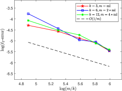
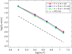
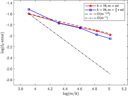
Figure 1: In 1bCS, PGD achieves error rates $\tilde{O}(\frac{k}{m})$ for $\mathbf{x}\in\Sigma^{n}_{k}$ (left), $\tilde{O}(\frac{\bar{r}(n_{1}+n_{2})}{m})$ for $\mathbf{x}\in M^{n_{1},n_{2}}_{\bar{r}}$ (middle), and $\tilde{O}((\frac{k}{m})^{1/3})$ for $\mathbf{x}\in\sqrt{k}\mathbb{B}_{1}^{n}\cap\mathbb{S}^{n-1}$ (right). In sparse recovery, we recover $k$-sparse $500$-dimensional signals under $m=c\cdot\text{ml}$ with $\text{ml}=400:200:1200$. In low-rank recovery, we recover rank-$\bar{r}$ $25\times 25$ matrices under $m=c\cdot\text{ml}$ with $\text{ml}=400:200:1200$. In recovering effectively sparse signals, we test $300$-dimensional signals under $m=c\cdot\text{ml}$ with $\text{ml}=800:400:2400$.

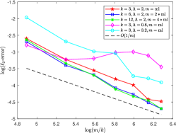
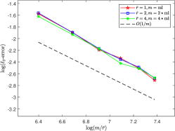
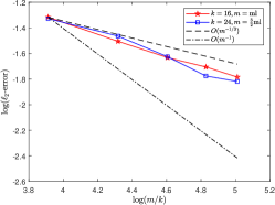
Figure 2: In D1bCS, PGD achieves error rates $\tilde{O}(\frac{k}{m})$ for $\mathbf{x}\in\Sigma^{n}_{k}$ (left), $\tilde{O}(\frac{\bar{r}(n_{1}+n_{2})}{m})$ for $\mathbf{x}\in M^{n_{1},n_{2}}_{\bar{r}}$ (middle), and $\tilde{O}((\frac{k}{m})^{1/3})$ for $\mathbf{x}\in\sqrt{k}\mathbb{B}_{1}^{n}\cap\mathbb{S}^{n-1}$ (right). In sparse recovery, we recover $k$-sparse $500$-dimensional signals under $m=c\cdot\text{ml}$ with $\text{ml}=400:200:1600$. In low-rank recovery, we recover rank-$\bar{r}$ $25\times 25$ matrices under measurement number $m=c\cdot\text{ml}$ with $\text{ml}=600:200:1600$ with $\Lambda=1.5$. In recovering effectively sparse signals, we test $300$-dimensional signals under $m=c\cdot\text{ml}$ with $\text{ml}=800:400:2400$.

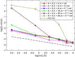
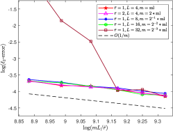
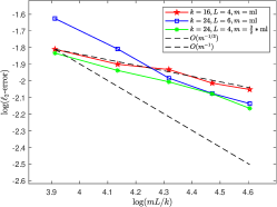
Figure 3: In DMbCS with $\delta=\frac{5}{L}$, PGD achieves error rates $\tilde{O}(\frac{k}{mL})$ for $\mathbf{x}\in\Sigma^{n}_{k}$ (left), $\tilde{O}(\frac{\bar{r}(n_{1}+n_{2})}{mL})$ for $\mathbf{x}\in M^{n_{1},n_{2}}_{\bar{r}}$ (middle), and $\tilde{O}((\frac{k}{mL})^{1/3})$ for $\mathbf{x}\in\sqrt{k}\mathbb{B}_{1}^{n}\cap\mathbb{S}^{n-1}$ (right). In sparse recovery, we recover $k$-sparse $500$-dimensional signals under measurement number $m=c\cdot\text{ml}$ with $\text{ml}=200:200:1200$. In low-rank recovery, we recover rank-$\bar{r}$ $25\times 25$ matrices under measurement number $m=c\cdot\text{ml}$ with $\text{ml}=1800:200:2800$. In recovering effectively sparse signals, we test $400$-dimensional signals under $m=c\cdot\text{ml}$ with $\text{ml}=800:200:1600$.

6 Discussions

The goal of quantized compressed sensing is to recover structured signals $\mathbf{x}$ from only a few quantized compressive measurements. The information-theoretic lower bounds for recovering $k$-sparse signals are known from the seminal work [18]: observing $\mathbf{y}=\mathcal{Q}(\mathbf{A}\mathbf{x}-\bm{\tau})$ under some $(\mathbf{A},\tau)\in\mathbb{R}^{m\times(n+1)}$ and $L$-level quantizer $\mathcal{Q}$, no algorithm achieves error rate faster than $\tilde{O}(\frac{k}{mL})$. However, most efficient algorithms in the literature are sub-optimal and only achieve error rates inferior to $\tilde{O}(\frac{1}{L}(\frac{k}{m})^{1/2})$. The only exception is NBIHT that was recently shown [21] to be near-optimal for 1bCS of $k$-sparse signals. Moreover, for recovering the effectively sparse signals in $\sqrt{k}\mathbb{B}_{1}^{n}$, the best known error rate, including that for the intractable HDM, is at the order $\tilde{O}((\frac{k}{mL})^{1/3})$. In this work, we provide a unified treatment to the general quantized compressed sensing problem by analyzing a PGD algorithm. An intriguing finding is that PGD is a computational procedure that achieves the same error rate as HDM under a set of conditions. By validating these conditions for the popular models 1bCS, D1bCS and DMbCS, we establish error rates for PGD that improve on or match the faster error rates in all instances.

It is worth discussing the robustness of PGD to noise or corruption. In a follow-up work of [21], the same authors showed [22] that NBIHT achieves error rate $\tilde{O}(\frac{k}{m}+\bar{\zeta})$ under a $\bar{\zeta}$-fraction of adversarial bit flips, that is, a setting where one observes $\mathbf{y}_{\rm cor}$ obeying $d_{H}(\mathbf{y}_{\rm cor},\operatorname{sign}(\mathbf{A}\mathbf{x}))\leq\bar{\zeta}m$. Under the same corruption pattern, Adaboost achieves $\tilde{O}((\frac{k}{m}+\bar{\zeta})^{1/3})$ for signals in $\sqrt{k}\mathbb{B}_{1}^{n}\cap\mathbb{S}^{n-1}$, as shown in [8, Corollary 2.3]. We shall note that the robustness to adversarial bit flips is in fact a straightforward extension of the current corruption-free results. Suppose that we observe $\mathbf{y}_{\rm cor}=\mathbf{y}+\mathbf{e}$ under the corruption $\mathbf{e}=(e_{1},\cdots,e_{m})^{\top}$, then the update rule of PGD reads

$$\mathbf{x}^{(t)}=\mathcal{P}_{\mathbbm{A}_{\alpha}^{\beta}}\left(\mathcal{P}_{\mathcal{K}}\Big{(}\mathbf{x}^{(t-1)}-\eta\cdot\mathbf{h}(\mathbf{x}^{(t-1)},\mathbf{x})-\frac{\eta\cdot\mathbf{A}^{\top}\mathbf{e}}{m}\Big{)}\right).$$ (58)

Since $\phi=r$ in Theorem 5 and an adapted RAIC similarly leads to convergence of PGD, we find that there is an additional term $O\big{(}\frac{\eta}{mr}\|\mathbf{A}^{\top}\mathbf{e}\|_{\mathcal{K}^{\circ}_{(r)}}\big{)}$ contributing to the estimation error. Let us characterize the corruption jointly by its sparsity and $\ell_{2}$-norm:

$$\|\mathbf{e}\|_{0}\leq\bar{\zeta}m\quad\text{and}\quad\|\mathbf{e}\|_{2}\leq\bar{\gamma}\sqrt{m}.$$

Then, Lemma 8, together with the sample complexity in Theorem 5, establishes the high-probability event

$$\frac{\eta}{mr}\|\mathbf{A}^{\top}\mathbf{e}\|_{\mathcal{K}^{\circ}_{(r)}}=\frac{\eta}{mr}\sup_{\mathbf{w}\in\mathcal{K}_{(r)}}\sum_{i=1}^{m}e_{i}\mathbf{a}_{i}^{\top}\mathbf{w}$$

$$\leq\frac{\eta}{m}\sup_{\mathbf{w}\in r^{-1}\mathcal{K}_{(r)}}\max_{\begin{subarray}{c}I\subset[m]\\ |I|\leq\bar{\zeta}m\end{subarray}}\sum_{i\in I}e_{i}|\mathbf{a}_{i}^{\top}\mathbf{w}|\leq\frac{\eta\|\mathbf{e}\|_{2}}{m}\sup_{\mathbf{w}\in r^{-1}\mathcal{K}_{(r)}}\max_{\begin{subarray}{c}I\subset[m]\\ |I|\leq\bar{\zeta}m\end{subarray}}\Big{(}\sum_{i\in I}|\mathbf{a}_{i}^{\top}\mathbf{w}|^{2}\Big{)}^{1/2}$$

$$\lesssim\frac{\eta\bar{\gamma}\cdot\omega(\mathcal{K}_{(r)})}{\sqrt{m}r}+\eta\bar{\gamma}\sqrt{\bar{\zeta}\log(\bar{\zeta}^{-1})}\lesssim\eta\bar{\gamma}\sqrt{\frac{r}{\Delta\vee\Lambda}}+\eta\bar{\gamma}\sqrt{\bar{\zeta}\log(\bar{\zeta}^{-1})}.$$

For 1bCS, we can always set $\bar{\gamma}=(2\bar{\zeta})^{1/2}$; combined with $(r\bar{\zeta})^{1/2}\leq 2r+2\bar{\gamma}$, we find that the corruption only increments the estimation error by $O(\bar{\zeta}\log^{1/2}(\bar{\zeta}^{-1}))$. This recovers the major result in [22], as well as improves on the $O(\bar{\zeta}^{1/3})$ dependence for Adaboost [8]. The robustness to pre-quantization noise which corrupts $\mathbf{y}$ to $\mathbf{y}_{\rm cor}:=\mathcal{Q}(\mathbf{A}\mathbf{x}-\bm{\tau}-\mathbf{e})$ seems more challenging. We leave this for future work and refer interested readers to the relevant treatments in [10, 19].

As most prior works, we focused on recovering signals that are exactly $k$-sparse or live in $\sqrt{k}\mathbb{B}_{1}^{n}$. To bridge these two cases together, we can characterize the approximate sparsity via $\ell_{q}$-norm ($q\in(0,1]$) and assume $\mathbf{x}\in\mathcal{K}:=k^{\frac{1}{q}-\frac{1}{2}}\mathbb{B}_{q}^{n}=\{\mathbf{u}\in\mathbb{R}^{n}:\sum_{i\in[n]}|u_{i}|^{q}\leq k^{1-\frac{q}{2}}\}$. By known estimates on the metric entropy of $\ell_{q}$-ball and Dudley’s inequality, our Theorem 5 implies that PGD achieves error rate $\tilde{O}((\frac{k}{m})^{\frac{2-q}{2+q}})$ over approximately sparse signals living in the scaled $\ell_{q}$-ball. This establishes an interesting phenomenon: by increasing $q$ from $0$ to $1$, the PGD error rate continuously decreases while the signal set $k^{\frac{1}{q}-\frac{1}{2}}\mathbb{B}_{q}^{n}\cap\mathbb{S}^{n-1}$ continuously “increases” in terms of inclusion. The caveat here is that the projection onto $\ell_{q}$-ball with $q\in(0,1)$ is difficult to compute, but we believe this finding is of interest in light of some existing heuristic for approximating such projection (e.g., [36]). We also note in passing [3] who analyzed the performance of $\ell_{q}$-PGD for linear compressed sensing.

We mention a few questions that need further investigation. An important direction for future work is to develop information-theoretic lower bound for the approximately sparse cases. For example, the rate $\tilde{O}((\frac{k}{m})^{1/3})$ is the best known rate for recovering signals in $\sqrt{k}\mathbb{B}_{1}^{n}$, but it remains unclear whether this is tight in any sense, as we discussed in Remark 2. Moreover, the current analysis is built upon sub-Gaussian sensing matrix. It is of great interest to relax this assumption to fit better with the sensing matrix in actual signal processing applications, or the features in machine learning problems.

Appendix

Appendix A Quantized Embedding Property

The general $L$-level quantizer (1) associated with some $(\mathbf{a},\tau)$ forms the quantized sampler $\mathcal{Q}(\langle\mathbf{a},\cdot\rangle-\tau)$.

A.1 Preparations

We will need the notions of (well) separation. A hyperplane $\mathcal{H}_{\mathbf{a},\tau}:=\{\mathbf{p}\in\mathbb{R}^{n}:\mathbf{a}^{\top}\mathbf{p}-\tau=0\}$ separates the whole space $\mathbb{R}^{n}$ into two sides:

$$\mathcal{H}_{\mathbf{a},\tau}^{+}=\{\mathbf{p}\in\mathbb{R}^{n}:\mathbf{a}^{\top}\mathbf{p}\geq\tau\}~{}~{}\text{and}~{}~{}\mathcal{H}^{-}_{\mathbf{a},\tau}=\{\mathbf{p}\in\mathbb{R}^{n}:\mathbf{a}^{\top}\mathbf{p}<\tau\}.$$

We say two points $\mathbf{u},\mathbf{v}$ are separated by $\mathcal{H}_{\mathbf{a},\tau}$ if they live in different sides of the hyperplane, which is a geometric statement equivalent to $\operatorname{sign}(\mathbf{a}^{\top}\mathbf{u}-\tau)\neq\operatorname{sign}(\mathbf{a}^{\top}\mathbf{v}-\tau)$. To build this viewpoint for the $L$-level quantizer (1), we note that $\mathcal{Q}(\mathbf{a}^{\top}\mathbf{u}-\tau)\neq\mathcal{Q}(\mathbf{a}^{\top}\mathbf{v}-\tau)$ happens if and only if $\operatorname{sign}(\mathbf{a}^{\top}\mathbf{u}-\tau-b_{j})\neq\operatorname{sign}(\mathbf{a}^{\top}\mathbf{v}-\tau-b_{j})$ holds for some $j\in[L-1]$. Hence, when associated with certain $(\mathbf{a},\tau)$, the $L$-level quantizer corresponds to $L-1$ hyperplanes $\{\mathcal{H}_{\mathbf{a},\tau+b_{j}}:j\in[L-1]\}$; geometrically, $\mathcal{Q}(\mathbf{a}^{\top}\mathbf{u}-\tau)\neq\mathcal{Q}(\mathbf{a}^{\top}\mathbf{v}-\tau)$ holds if and only if $\mathbf{u},\mathbf{v}$ are separated by $\mathcal{H}_{\mathbf{a},\tau+b_{j}}$ for some $j\in[L-1]$. Such separation, however, can be unstable: suppose that $\mathbf{u}\in\mathcal{H}_{\mathbf{a},\tau}^{+}$ and $\mathbf{v}\in\mathcal{H}_{\mathbf{a},\tau}^{-}$ live very close to the hyperplane itself $\mathcal{H}_{\mathbf{a},\tau}$, then $\mathcal{H}_{\mathbf{a},\tau}$ may no longer separate $\mathbf{u}^{\prime}$ and $\mathbf{v}$ even though $\mathbf{u}^{\prime}$ and $\mathbf{u}$ are very close. As with [28, 10, 19, 7], we shall work with $\theta$-well-separation.

Definition 2.

In the context of quantized compressed sensing under the quantizer (1) with resolution $\Delta$, we say $\mathcal{H}_{\mathbf{a},\tau}$ $\theta$-well-separates $\mathbf{u}$ and $\mathbf{v}$ if $\mathcal{H}_{\mathbf{a},\tau}$ separates $\mathbf{u}$ and $\mathbf{v}$, and it holds additionally that

$$\min\big{\{}|\mathbf{a}^{\top}\mathbf{u}-\tau|,|\mathbf{a}^{\top}\mathbf{v}-\tau|\big{\}}\geq\theta\min\{\|\mathbf{u}-\mathbf{v}\|_{2},\Delta\}.$$

Definition 3.

Consider the quantizer (1) associated with certain $(\mathbf{a},\tau)$, we say the quantized sampler $\mathcal{Q}(\langle\mathbf{a},\cdot\rangle-\tau)$ distinguishes ($\theta$-well-distinguishes, resp.) $\mathbf{u}$ and $\mathbf{v}$, if there exists some $j\in[L-1]$ such that $\mathcal{H}_{\mathbf{a},\tau+b_{j}}$ separates ($\theta$-well-separates, resp.) $\mathbf{u}$ and $\mathbf{v}$. In particular, $\mathcal{Q}(\langle\mathbf{a},\cdot\rangle-\tau)$ distinguishes $\mathbf{u},\mathbf{v}$ if and only if $\mathcal{Q}(\mathbf{a}^{\top}\mathbf{u}-\tau)\neq\mathcal{Q}(\mathbf{a}^{\top}\mathbf{v}-\tau)$.

Next, we present two useful facts.

Lemma 2.

Given $\mathbf{u}$ and $\mathbf{v}$, if

$$\min_{j\in[L-1]}|\mathbf{a}^{\top}\mathbf{u}-\tau-b_{j}|>2|\mathbf{a}^{\top}(\mathbf{u}-\mathbf{v})|,$$ (59)

then $\mathbf{u}$ and $\mathbf{v}$ are not distinguished by $\mathcal{Q}(\langle\mathbf{a},\cdot\rangle-\tau)$, i.e., $\mathcal{Q}(\mathbf{a}^{\top}\mathbf{u}-\tau)=\mathcal{Q}(\mathbf{a}^{\top}\mathbf{v}-\tau)$.

Proof.

We shall assume $\mathbf{u},\mathbf{v}$ are distinguished by $\mathcal{Q}(\langle\mathbf{a},\cdot\rangle-\tau)$ and seek a contradiction. Particularly, suppose $\mathcal{Q}(\mathbf{a}^{\top}\mathbf{u}-\tau)\neq\mathcal{Q}(\mathbf{a}^{\top}\mathbf{v}-\tau)$, then there exists some $j\in[L-1]$ such that $\mathcal{H}_{\mathbf{a},\tau+b_{j}}$ separates $\mathbf{u}$ and $\mathbf{v}$, namely, $\operatorname{sign}(\mathbf{a}^{\top}\mathbf{u}-\tau-b_{j})\neq\operatorname{sign}(\mathbf{a}^{\top}\mathbf{v}-\tau-b_{j})$. This leads to

$$|\mathbf{a}^{\top}(\mathbf{u}-\mathbf{v})|=\big{|}(\mathbf{a}^{\top}\mathbf{u}-\tau-b_{j})-(\mathbf{a}^{\top}\mathbf{v}-\tau-b_{j})\big{|}\geq|\mathbf{a}^{\top}\mathbf{u}-\tau-b_{j}|,$$

which contradicts (59). ∎

Lemma 3.

Given $\mathbf{u},\mathbf{v},\mathbf{p},\mathbf{q}$ and some $\theta>0$, if $\mathcal{Q}(\langle\mathbf{a},\cdot\rangle-\tau)$ $\theta$-well-distinguishes $\mathbf{u}$ and $\mathbf{v}$, and additionally

$$\max\big{\{}|\mathbf{a}^{\top}(\mathbf{p}-\mathbf{u})|,|\mathbf{a}^{\top}(\mathbf{q}-\mathbf{v})|\big{\}}<\frac{\theta}{2}\min\{\|\mathbf{u}-\mathbf{v}\|_{2},\Delta\},$$ (60)

then $\mathbf{p}$ and $\mathbf{q}$ are distinguished by $\mathcal{Q}(\langle\mathbf{a},\cdot\rangle-\tau)$, i.e., $\mathcal{Q}(\mathbf{a}^{\top}\mathbf{p}-\tau)\neq\mathcal{Q}(\mathbf{a}^{\top}\mathbf{q}-\tau)$.

Proof.

By Definition 3, for some $j\in[L-1]$ we have $\operatorname{sign}(\mathbf{a}^{\top}\mathbf{u}-\tau-b_{j})\neq\operatorname{sign}(\mathbf{a}^{\top}\mathbf{v}-\tau-b_{j})$ and

$$\min\big{\{}|\mathbf{a}^{\top}\mathbf{u}-\tau-b_{j}|,|\mathbf{a}^{\top}\mathbf{v}-\tau-b_{j}|\big{\}}\geq\theta\min\{\|\mathbf{u}-\mathbf{v}\|_{2},\Delta\}.$$

Combining with (60) we obtain

$$2|\mathbf{a}^{\top}(\mathbf{p}-\mathbf{u})|<|\mathbf{a}^{\top}\mathbf{u}-\tau-b_{j}|,$$

$$2|\mathbf{a}^{\top}(\mathbf{q}-\mathbf{v})|<|\mathbf{a}^{\top}\mathbf{v}-\tau-b_{j}|.$$

Now we invoke Lemma 2 with respect to the 1-bit quantized sampler $\operatorname{sign}(\langle\mathbf{a},\cdot\rangle-\tau-b_{j})$, yielding that it does not distinguish $\mathbf{u}$ and $\mathbf{p}$, nor $\mathbf{v}$ and $\mathbf{q}$. We hence arrive at $\operatorname{sign}(\mathbf{a}^{\top}\mathbf{p}-\tau-b_{j})=\operatorname{sign}(\mathbf{a}^{\top}\mathbf{u}-\tau-b_{j})$ and $\operatorname{sign}(\mathbf{a}^{\top}\mathbf{q}-\tau-b_{j})=\operatorname{sign}(\mathbf{a}^{\top}\mathbf{v}-\tau-b_{j})$. Taken collectively with $\operatorname{sign}(\mathbf{a}^{\top}\mathbf{u}-\tau-b_{j})\neq\operatorname{sign}(\mathbf{a}^{\top}\mathbf{v}-\tau-b_{j})$, we obtain $\operatorname{sign}(\mathbf{a}^{\top}\mathbf{p}-\tau-b_{j})\neq\operatorname{sign}(\mathbf{a}^{\top}\mathbf{q}-\tau-b_{j})$ that implies the desired $\mathcal{Q}(\mathbf{a}^{\top}\mathbf{p}-\tau)\neq\mathcal{Q}(\mathbf{a}^{\top}\mathbf{q}-\tau)$. ∎

A.2 The Proof of Theorem 2 (Quantized Embedding Property)

We now delve into the arguments for proving Theorem 2. For some $r\in(0,c_{0}\Delta)$ with small enough $c_{0}$, we let $r^{\prime}=\frac{c_{1}r}{\log^{1/2}(\frac{\Delta\vee\Lambda}{r})}$ for some small enough constant $c_{1}$. We construct $\mathcal{N}_{r^{\prime}}$ as a minimal $r^{\prime}$-net of $\mathcal{W}$ that satisfies $\log|\mathcal{N}_{r^{\prime}}|=\mathscr{H}(\mathcal{W},r^{\prime})$. For any $\mathbf{u},\mathbf{v}\in\mathcal{W}$, we find their closest points in $\mathcal{N}_{r^{\prime}}$ as follows:

$$\mathbf{p}=\text{arg}\min_{\mathbf{w}\in\mathcal{N}_{r^{\prime}}}\|\mathbf{w}-\mathbf{u}\|_{2}~{}~{}\text{and}~{}~{}\mathbf{q}=\text{arg}\min_{\mathbf{w}\in\mathcal{N}_{r^{\prime}}}\|\mathbf{w}-\mathbf{v}\|_{2}.$$ (61)

(i) Establish the event $E_{s}$

Given any $\mathbf{u},\mathbf{v}\in\mathcal{W}$ obeying $\|\mathbf{u}-\mathbf{v}\|_{2}\leq r^{\prime}/2$, we have $\|\mathbf{u}-\mathbf{p}\|_{2}\leq r^{\prime}$ and $\|\mathbf{v}-\mathbf{p}\|_{2}\leq\|\mathbf{v}-\mathbf{u}\|_{2}+\|\mathbf{u}-\mathbf{p}\|_{2}\leq 3r^{\prime}/2$. By Lemma 2 and a union bound, we can proceed with the following deterministic arguments:

$$m-d_{H}\big{(}\mathcal{Q}(\mathbf{A}\mathbf{u}-\bm{\tau}),\mathcal{Q}(\mathbf{A}\mathbf{p}-\bm{\tau})\big{)}=\sum_{i=1}^{m}\mathbbm{1}\big{(}\mathcal{Q}(\mathbf{a}_{i}^{\top}\mathbf{u}-\tau_{i})=\mathcal{Q}(\mathbf{a}_{i}^{\top}\mathbf{p}-\tau_{i})\big{)}$$

$$\geq\sum_{i=1}^{m}\mathbbm{1}\Big{(}\min_{j\in[L-1]}|\mathbf{a}_{i}^{\top}\mathbf{p}-\tau_{i}-b_{j}|>r,~{}|\mathbf{a}_{i}^{\top}(\mathbf{u}-\mathbf{p})|\leq\frac{r}{2}\Big{)}$$

$$\geq\sum_{i=1}^{m}\mathbbm{1}\Big{(}\min_{j\in[L-1]}|\mathbf{a}_{i}^{\top}\mathbf{p}-\tau_{i}-b_{j}|>r\Big{)}-\sum_{i=1}^{m}\mathbbm{1}\Big{(}|\mathbf{a}_{i}^{\top}(\mathbf{u}-\mathbf{p})|>\frac{r}{2}\Big{)},$$

which imply

$$d_{H}\big{(}\mathcal{Q}(\mathbf{A}\mathbf{u}-\bm{\tau}),\mathcal{Q}(\mathbf{A}\mathbf{p}-\bm{\tau})\big{)}\leq\sum_{i=1}^{m}\mathbbm{1}\Big{(}\min_{j\in[L-1]}|\mathbf{a}_{i}^{\top}\mathbf{p}-\tau_{i}-b_{j}|\leq r\Big{)}+\sum_{i=1}^{m}\mathbbm{1}\Big{(}|\mathbf{a}_{i}^{\top}(\mathbf{u}-\mathbf{p})|>\frac{r}{2}\Big{)}.$$

This remains valid when replacing $\mathbf{u}$ with $\mathbf{v}$, hence we have

$$d_{H}\big{(}\mathcal{Q}(\mathbf{A}\mathbf{v}-\bm{\tau}),\mathcal{Q}(\mathbf{A}\mathbf{p}-\bm{\tau})\big{)}\leq\sum_{i=1}^{m}\mathbbm{1}\Big{(}\min_{j\in[L-1]}|\mathbf{a}_{i}^{\top}\mathbf{p}-\tau_{i}-b_{j}|\leq r\Big{)}+\sum_{i=1}^{m}\mathbbm{1}\Big{(}|\mathbf{a}_{i}^{\top}(\mathbf{v}-\mathbf{p})|>\frac{r}{2}\Big{)}.$$

Noticing $\mathbf{p}\in\mathcal{N}_{r^{\prime}}$ and $\mathbf{u}-\mathbf{p},\mathbf{v}-\mathbf{p}\in\mathcal{W}_{(3r^{\prime}/2)}$, by triangle inequality and taking supremums, we arrive at

$$d_{H}\big{(}\mathcal{Q}(\mathbf{A}\mathbf{u}-\bm{\tau}),\mathcal{Q}(\mathbf{A}\mathbf{v}-\bm{\tau})\big{)}$$

$$\leq d_{H}\big{(}\mathcal{Q}(\mathbf{A}\mathbf{u}-\bm{\tau}),\mathcal{Q}(\mathbf{A}\mathbf{p}-\bm{\tau})\big{)}+d_{H}\big{(}\mathcal{Q}(\mathbf{A}\mathbf{v}-\bm{\tau}),\mathcal{Q}(\mathbf{A}\mathbf{p}-\bm{\tau})\big{)}$$

$$\leq 2\sum_{i=1}^{m}\mathbbm{1}\Big{(}\min_{j\in[L-1]}|\mathbf{a}_{i}^{\top}\mathbf{p}-\tau_{i}-b_{j}|\leq r\Big{)}+\sum_{i=1}^{m}\mathbbm{1}\Big{(}|\mathbf{a}_{i}^{\top}(\mathbf{u}-\mathbf{p})|>\frac{r}{2}\Big{)}+\sum_{i=1}^{m}\mathbbm{1}\Big{(}|\mathbf{a}_{i}^{\top}(\mathbf{v}-\mathbf{p})|>\frac{r}{2}\Big{)}$$

$$\leq 2\underbrace{\sup_{\mathbf{p}\in\mathcal{N}_{r^{\prime}}}\sum_{i=1}^{m}\mathbbm{1}\Big{(}\min_{j\in[L-1]}|\mathbf{a}_{i}^{\top}\mathbf{p}-\tau_{i}-b_{j}|\leq r\Big{)}}_{:=\breve{T}_{1}}+2\underbrace{\sup_{\mathbf{w}\in\mathcal{W}_{(3r^{\prime}/2)}}\sum_{i=1}^{m}\mathbbm{1}\Big{(}|\mathbf{a}_{i}^{\top}\mathbf{w}|>\frac{r}{2}\Big{)}}_{:=\breve{T}_{2}}.$$ (62)

To bound $\breve{T}_{1}$, we shall invoke Chernoff bound along with a union bound. By Assumption 2, for any $\mathbf{p}\in\mathcal{N}_{r^{\prime}}$, $\min_{j\in[L-1]}|\mathbf{a}_{i}^{\top}\mathbf{p}-\tau_{i}-b_{j}|\leq r$ holds with probability smaller than $\frac{c^{(1)}r}{\Delta\vee\Lambda}$, hence we have

$$\mathbbm{P}\Big{(}\sum_{i=1}^{m}\mathbbm{1}\Big{(}\min_{j\in[L-1]}|\mathbf{a}_{i}^{\top}\mathbf{p}-\tau_{i}-b_{j}|\leq r\Big{)}\geq\frac{3mc^{(1)}r}{2(\Delta\vee\Lambda)}\Big{)}$$

$$\leq\mathbbm{P}\Big{(}\text{Bin}\Big{(}m,\frac{c^{(1)}r}{\Delta\vee\Lambda}\Big{)}\geq\frac{2mc^{(1)}r}{\Delta\vee\Lambda}\Big{)}\leq\exp\Big{(}-\frac{c^{(1)}}{12}\frac{mr}{\Delta\vee\Lambda}\Big{)},$$

where the last inequality is due to (133) in Lemma 7. Hence, a union bound shows that $\breve{T}_{1}\leq\frac{3c^{(1)}mr}{2(\Delta\vee\Lambda)}$ holds with probability at least

$$1-\exp\Big{(}\mathscr{H}(\mathcal{W},r^{\prime})-\frac{c^{(1)}}{12}\frac{mr}{\Delta\vee\Lambda}\Big{)}\geq 1-\exp\Big{(}-\frac{c^{(1)}}{24}\frac{mr}{\Delta\vee\Lambda}\Big{)},$$

with the proviso that $m\geq\frac{24(\Delta\vee\Lambda)}{c^{(1)}}\frac{\mathscr{H}(\mathcal{W},r^{\prime})}{r}$, which has been assumed in (11) in our statement.

We seek to control $\breve{T}_{2}$ to a scaling similar to the bound for $\breve{T}_{1}$. In particular, we seek to show $\breve{T}_{2}\leq\frac{c^{\prime}mr}{\Delta\vee\Lambda}$ for some constant $c^{\prime}$ such that $\frac{c^{\prime}r}{\Delta\vee\Lambda}<1$; here, $c^{\prime}$ is independent of other constants and can be set small enough if needed. To this end, we let $\ell_{0}:=\lceil\frac{c^{\prime}mr}{\Delta\vee\Lambda}\rceil$ and observe that it is sufficient to ensure

$$\sup_{\mathbf{w}\in\mathcal{W}_{(3r^{\prime}/2)}}\max_{\begin{subarray}{c}I\subset[m]\\ |I|\leq\ell_{0}\end{subarray}}\Big{(}\frac{1}{\ell_{0}}\sum_{i\in I}|\mathbf{a}_{i}^{\top}\mathbf{w}|^{2}\Big{)}^{1/2}\leq\frac{r}{2}.$$

By Lemma 8, with probability at least $1-2\exp(-\frac{c^{\prime}mr}{\Delta\vee\Lambda})$, we only need to ensure

$$\frac{\omega(\mathcal{W}_{(3r^{\prime}/2)})}{\sqrt{\ell_{0}}}+\frac{3r^{\prime}}{2}\log^{1/2}\Big{(}\frac{em}{\ell_{0}}\Big{)}\leq c_{3}r$$

for some small enough absolute constant $c_{3}$; note that this follows from (11) and our choice $r^{\prime}=\frac{cr}{\log^{1/2}(\frac{\Delta\vee\Lambda}{r})}$ with small enough $c$. Substituting the bounds on $\breve{T_{1}}$ and $\breve{T}_{2}$ into (62), we have shown that the event $E_{s}$ holds with the promised probability.

(ii) Establish the event $E_{l}$

With Assumptions 2–3, we let $c^{(0)}:=\min\{\frac{c^{(2)}}{4c^{(1)}},\frac{1}{4}\}$ and first establish a lower bound on the probability of $\mathbf{u}$ and $\mathbf{v}$ being $c^{(0)}$-well-distinguished by $\mathcal{Q}(\langle\mathbf{a}_{i},\cdot\rangle-\tau_{i})$:

$$\mathbbm{P}\Big{(}\mathcal{Q}(\langle\mathbf{a}_{i},\cdot\rangle-\tau_{i})~{}\text{$c^{(0)}$-well-distinguishes }\mathbf{u}\text{ and }\mathbf{v}\Big{)}$$

$$\geq\mathbbm{P}\big{(}\mathcal{Q}(\mathbf{a}_{i}^{\top}\mathbf{u}-\tau_{i})\neq\mathcal{Q}(\mathbf{a}_{i}^{\top}\mathbf{v}-\tau_{i})\big{)}$$

$$\qquad\qquad-\mathbbm{P}\Big{(}\min_{j\in[L-1]}\min\{|\mathbf{a}_{i}^{\top}\mathbf{u}-\tau_{i}-b_{j}|,|\mathbf{a}_{i}^{\top}\mathbf{v}-\tau_{i}-b_{j}|\}<c^{(0)}\min\{\|\mathbf{u}-\mathbf{v}\|_{2},\Delta\}\Big{)}$$

$$\geq\mathbbm{P}\big{(}\mathcal{Q}(\mathbf{a}_{i}^{\top}\mathbf{u}-\tau_{i})\neq\mathcal{Q}(\mathbf{a}_{i}^{\top}\mathbf{v}-\tau_{i})\big{)}-\mathbbm{P}\Big{(}\min_{j\in[L-1]}|\mathbf{a}_{i}^{\top}\mathbf{u}-\tau_{i}-b_{j}|<c^{(0)}\min\{\|\mathbf{u}-\mathbf{v}\|_{2},\Delta\}\Big{)}$$

$$\qquad\qquad-\mathbbm{P}\Big{(}\min_{j\in[L-1]}|\mathbf{a}_{i}^{\top}\mathbf{v}-\tau_{i}-b_{j}|<c^{(0)}\min\{\|\mathbf{u}-\mathbf{v}\|_{2},\Delta\}\Big{)}$$

$$\geq c^{(2)}\min\Big{\{}\frac{\|\mathbf{u}-\mathbf{v}\|_{2}}{\Delta\vee\Lambda},1\Big{\}}-\frac{2c^{(1)}c^{(0)}\min\{\|\mathbf{u}-\mathbf{v}\|_{2},\Delta\}}{\Delta\vee\Lambda}$$

$$\geq\frac{c^{(2)}}{2}\min\Big{\{}\frac{\|\mathbf{u}-\mathbf{v}\|_{2}}{\Delta\vee\Lambda},1\Big{\}}.$$ (63)

For any $(\mathbf{u},\mathbf{v})\in\mathcal{W}\times\mathcal{W}$ obeying $\|\mathbf{u}-\mathbf{v}\|_{2}\geq 2r$ and the corresponding $\mathbf{p},\mathbf{q}$ found by (61), by $r^{\prime}<r/2$ we have

$$\|\mathbf{p}-\mathbf{q}\|_{2}\geq\|\mathbf{u}-\mathbf{v}\|_{2}-\|\mathbf{u}-\mathbf{p}\|_{2}-\|\mathbf{v}-\mathbf{q}\|_{2}\geq\frac{\|\mathbf{u}-\mathbf{v}\|_{2}}{2}\geq r,$$ (64)

where the second inequality holds because $\|\mathbf{u}-\mathbf{p}\|_{2}+\|\mathbf{v}-\mathbf{q}\|_{2}\leq 2r^{\prime}<r\leq\frac{1}{2}\|\mathbf{u}-\mathbf{v}\|_{2}$. Then by Lemma 3, along with $\min\{\|\mathbf{p}-\mathbf{q}\|_{2},\Delta\}\geq r$, we proceed with the following deterministic arguments:

$$d_{H}\big{(}\mathcal{Q}(\mathbf{A}\mathbf{u}-\bm{\tau}),\mathcal{Q}(\mathbf{A}\mathbf{v}-\bm{\tau})\big{)}$$

$$\geq\sum_{i=1}^{m}\mathbbm{1}\Big{(}\mathcal{Q}(\langle\mathbf{a}_{i},\cdot\rangle-\tau_{i})~{}\text{$c^{(0)}$-well-distinguishes }\mathbf{p}\text{ and }\mathbf{q},~{}\max\{|\mathbf{a}_{i}^{\top}(\mathbf{u}-\mathbf{p})|,|\mathbf{a}_{i}^{\top}(\mathbf{v}-\mathbf{q})|\}\leq\frac{c^{(0)}r}{2}\Big{)}$$

$$\geq\sum_{i=1}^{m}\mathbbm{1}\big{(}\mathcal{Q}(\langle\mathbf{a}_{i},\cdot\rangle-\tau_{i})~{}\text{$c^{(0)}$-well-distinguishes }\mathbf{p}\text{ and }\mathbf{q}\big{)}$$ (65a)

$$\qquad\qquad\qquad-\sum_{i=1}^{m}\mathbbm{1}\Big{(}|\mathbf{a}_{i}^{\top}(\mathbf{u}-\mathbf{p})|\geq\frac{c^{(0)}r}{2}\Big{)}-\sum_{i=1}^{m}\mathbbm{1}\Big{(}|\mathbf{a}_{i}^{\top}(\mathbf{v}-\mathbf{q})|\geq\frac{c^{(0)}r}{2}\Big{)}.$$ (65b)

Let us denote the term in (65a) by $\breve{T}_{3}^{\mathbf{p},\mathbf{q}}$, and now we seek to lower bound $\breve{T}_{3}^{\mathbf{p},\mathbf{q}}$ uniformly for all $(\mathbf{p},\mathbf{q})\in\mathcal{U}_{r,r^{\prime}}:=\{(\mathbf{p},\mathbf{q})\in\mathcal{N}_{r^{\prime}}\times\mathcal{N}_{r^{\prime}}:\|\mathbf{p}-\mathbf{q}\|_{2}\geq r\}$. We first achieve this for a fixed pair $(\mathbf{p},\mathbf{q})\in\mathcal{U}_{r,r^{\prime}}$. By (63) and (134) in Lemma 7 we obtain that, for fixed $(\mathbf{p},\mathbf{q})\in\mathcal{U}_{r,r^{\prime}}$,

$$\mathbbm{P}\Big{(}\breve{T}_{3}^{\mathbf{p},\mathbf{q}}\leq\frac{c^{(2)}m}{4}\min\Big{\{}\frac{\|\mathbf{p}-\mathbf{q}\|_{2}}{\Delta\vee\Lambda},1\Big{\}}\Big{)}$$

$$\leq\mathbbm{P}\left(\text{Bin}\Big{(}m,\frac{c^{(2)}}{2}\min\Big{\{}\frac{\|\mathbf{p}-\mathbf{q}\|_{2}}{\Delta\vee\Lambda},1\Big{\}}\Big{)}\leq\frac{c^{(2)}m}{4}\min\Big{\{}\frac{\|\mathbf{p}-\mathbf{q}\|_{2}}{\Delta\vee\Lambda},1\Big{\}}\right)$$

$$\leq\exp\Big{(}-\frac{c^{(2)}m}{24}\min\Big{\{}\frac{\|\mathbf{p}-\mathbf{q}\|_{2}}{\Delta\vee\Lambda},1\Big{\}}\Big{)}\leq\exp\Big{(}-\frac{c^{(2)}mr}{24(\Delta\vee\Lambda)}\Big{)}.$$

Taking a union bound, $\breve{T}_{3}^{\mathbf{p},\mathbf{q}}>\frac{c^{(2)}m}{8}\min\big{\{}\frac{\|\mathbf{p}-\mathbf{q}\|_{2}}{\Delta\vee\Lambda},1\big{\}}$ holds for any $(\mathbf{p},\mathbf{q})\in\mathcal{U}_{r,r^{\prime}}$ with probability at least

$$1-\exp\Big{(}2\mathscr{H}(\mathcal{W},r^{\prime})-\frac{c^{(2)}mr}{24(\Delta\vee\Lambda)}\Big{)}\geq 1-\exp\Big{(}-\frac{c^{(2)}mr}{48(\Delta\vee\Lambda)}\Big{)},$$

with the proviso that $m\geq\frac{96(\Delta\vee\Lambda)}{c^{(2)}r}\mathscr{H}(\mathcal{W},r^{\prime})$; we assume this in (11).

Next, we bound the terms in (65b). By $\mathbf{u}-\mathbf{p},\mathbf{v}-\mathbf{q}\in\mathcal{W}_{(3r^{\prime}/2)}$, we have

$$\sum_{i=1}^{m}\mathbbm{1}\Big{(}|\mathbf{a}_{i}^{\top}(\mathbf{u}-\mathbf{p})|\geq\frac{c^{(0)}r}{2}\Big{)}+\sum_{i=1}^{m}\mathbbm{1}\Big{(}|\mathbf{a}_{i}^{\top}(\mathbf{v}-\mathbf{q})|\geq\frac{c^{(0)}r}{2}\Big{)}\leq 2\sup_{\mathbf{w}\in\mathcal{W}_{(3r^{\prime}/2)}}\sum_{i=1}^{m}\Big{(}|\mathbf{a}_{i}^{\top}\mathbf{w}|\geq\frac{c^{(0)}r}{2}\Big{)}:=2\breve{T}_{4}.$$

By arguments parallel to those for bounding $\breve{T}_{2}$, under (11) and $r^{\prime}=\frac{c_{1}r}{\log^{1/2}(\{\Delta\vee\Lambda\}/r)}$ with some $c_{1},C_{2}$ depending on $c^{(1)}$ and $c^{(2)}$, we can show $2\breve{T}_{4}\leq\frac{c^{(2)}mr}{16(\Delta\vee\Lambda)}$ with probability at least $1-\exp(-\frac{c^{\prime\prime}mr}{\Delta\vee\Lambda})$ for some $c^{\prime\prime}$ depending on $c^{(1)}$ and $c^{(2)}$.

Hence, we can substitute the bounds on $\breve{T}_{3}^{\mathbf{p},\mathbf{q}}$ and $\breve{T}_{4}$ into (65), yielding the following for any $(\mathbf{u},\mathbf{v})\in\mathcal{W}\times\mathcal{W}$ obeying $\|\mathbf{u}-\mathbf{v}\|_{2}\geq 2r$:

$$d_{H}\big{(}\mathcal{Q}(\mathbf{A}\mathbf{u}-\bm{\tau}),\mathcal{Q}(\mathbf{A}\mathbf{v}-\bm{\tau})\big{)}\geq\frac{c^{(2)}m}{4}\min\Big{\{}\frac{\|\mathbf{p}-\mathbf{q}\|_{2}}{\Delta\vee\Lambda},1\Big{\}}-\frac{c^{(2)}mr}{16(\Delta\vee\Lambda)}$$

$$\geq\frac{c^{(2)}m}{8}\min\Big{\{}\frac{\|\mathbf{p}-\mathbf{q}\|_{2}}{\Delta\vee\Lambda},1\Big{\}}\geq\frac{c^{(2)}m}{16}\min\Big{\{}\frac{\|\mathbf{u}-\mathbf{v}\|_{2}}{\Delta\vee\Lambda},1\Big{\}},$$

where the last inequality follows from $\|\mathbf{p}-\mathbf{q}\|_{2}\geq\frac{1}{2}\|\mathbf{u}-\mathbf{v}\|_{2}$, see (64). We have shown that the desired $E_{l}$ holds with the promised probability.

Appendix B The Proof of Theorem 4 (RAIC Implies Convergence)

We define

$$\hat{t}=\inf\big{\{}t\in\mathbb{Z}_{\geq 0}:\|\mathbf{x}^{(t)}-\mathbf{x}\|_{2}\leq E(\bm{\mu})\big{\}}$$

as the smallest $t$ such that $\mathbf{x}^{(t)}$ enters $\mathbb{B}_{2}^{n}(\mathbf{x};E(\bm{\mu}))$, with the convention that $\hat{t}=\infty$ if such $t$ does not exist.

(i) Showing $\hat{t}\leq\lceil\frac{\log(E(\bm{\mu})/\mu_{4})}{\log(1/2+\kappa_{\alpha}\mu_{1})}\rceil$

We assume $\|\mathbf{x}^{(0)}-\mathbf{x}\|_{2}>E(\bm{\mu})$, otherwise $\hat{t}=0$ and we are done. By $E(\bm{\mu})=\max\{\frac{64\kappa_{\alpha}^{2}\mu_{2}}{(1-2\kappa_{\alpha}\mu_{1})^{2}},\frac{8\kappa_{\alpha}\mu_{3}}{1-2\kappa_{\alpha}\mu_{1}}\}$ and $\|\mathbf{x}^{(0)}-\mathbf{x}\|_{2}>E(\bm{\mu})$ we obtain

$$2\kappa_{\alpha}\big{(}\mu_{2}\|\mathbf{x}^{(0)}-\mathbf{x}\|_{2}\big{)}^{1/2}\leq\frac{1-2\kappa_{\alpha}\mu_{1}}{4}\|\mathbf{x}^{(0)}-\mathbf{x}\|_{2}\quad\text{and}\quad 2\kappa_{\alpha}\mu_{3}\leq\frac{1-2\kappa_{\alpha}\mu_{1}}{4}\|\mathbf{x}^{(0)}-\mathbf{x}\|_{2}.$$ (66)

Hence, we can bound $\|\tilde{\mathbf{x}}^{(1)}-\mathbf{x}\|_{2}$ as

$$\|\tilde{\mathbf{x}}^{(1)}-\mathbf{x}\|_{2}=\big{\|}\mathcal{P}_{\mathcal{K}}(\mathbf{x}^{(0)}-\eta\cdot\mathbf{h}(\mathbf{x}^{(0)},\mathbf{x}))-\mathbf{x}\big{\|}_{2}$$ (67a)

$$\leq\max\Big{\{}\mu_{3},\frac{2}{\mu_{3}}\big{\|}\mathbf{x}^{(0)}-\mathbf{x}-\eta\cdot\mathbf{h}(\mathbf{x}^{(0)},\mathbf{x})\big{\|}_{\mathcal{K}_{(\mu_{3})}^{\circ}}\Big{\}}$$ (67b)

$$\leq 2\mu_{1}\|\mathbf{x}^{(0)}-\mathbf{x}\|_{2}+2(\mu_{2}\cdot\|\mathbf{x}^{(0)}-\mathbf{x}\|_{2})^{1/2}+2\mu_{3},$$ (67c)

where (67b) follows from Lemma 9, in (67c) we use $\mathbf{x},\mathbf{x}^{(0)}\in 2\mathcal{K}\cap\mathbbm{A}_{\alpha}^{\beta}$ and $(2\mathcal{K}\cap\mathbbm{A}_{\alpha}^{\beta},\bm{\mu})$-RAIC. We notice that $\mathbbm{A}_{\alpha}^{\beta}$ is convex if and only if $\alpha=0$, hence (e.g., by [31, Lemma 15]) we come to

$$\|\mathbf{x}^{(1)}-\mathbf{x}\|_{2}=\big{\|}\mathcal{P}_{\mathbbm{A}_{\alpha}^{\beta}}(\tilde{\mathbf{x}}^{(1)})-\mathbf{x}\big{\|}_{2}\leq\kappa_{\alpha}\|\tilde{\mathbf{x}}^{(1)}-\mathbf{x}\|_{2}.$$ (68)

Combining (66)–(68) yields $\|\mathbf{x}^{(1)}-\mathbf{x}\|_{2}\leq(\frac{1}{2}+\kappa_{\alpha}\mu_{1})\|\mathbf{x}^{(0)}-\mathbf{x}\|_{2}$. By $\kappa_{\alpha}\mu_{1}<\frac{1}{2}$ we have $\|\mathbf{x}^{(1)}-\mathbf{x}\|_{2}\leq\|\mathbf{x}^{(0)}-\mathbf{x}\|_{2}\leq\mu_{4},$ $\mathbf{x}^{(1)}\in\mathcal{K}$ and $\mathbb{B}(\mathbf{x};\mu_{4})\cap\mathcal{K}\subset\mathcal{X}$. Moreover, if $\mathcal{K}$ is a cone, since projection onto $\mathbbm{A}_{\alpha}^{\beta}$ only changes signal norms and $\tilde{\mathbf{x}}^{(1)}\in\mathcal{K}$, we have $\mathbf{x}^{(1)}\in\mathcal{K}$. Also, if $\alpha=0$, since projection onto $\mathbbm{A}_{\alpha}^{\beta}$ will not increase signal norm, and $\mathcal{K}$ is star-shaped, we have $\mathbf{x}^{(1)}\in\mathcal{K}$. On the other hand, if $\mathcal{K}$ is not a cone and $\alpha>0$, recall that we have additionally assumed (18), which together with (67) gives $\|\tilde{\mathbf{x}}^{(1)}-\mathbf{x}\|_{2}\leq 2\mu_{1}\mu_{4}+2\sqrt{\mu_{2}\mu_{4}}+2\mu_{3}\leq\frac{\alpha}{2}$; then, by triangle inequality and $\mathbf{x}\in\mathbbm{A}_{\alpha}^{\beta}$ we obtain $\|\tilde{\mathbf{x}}^{(1)}\|_{2}\geq\frac{\alpha}{2}$; thus, we have $\|\mathbf{x}^{(1)}\|_{2}\leq 2\|\tilde{\mathbf{x}}^{(1)}\|_{2}$ and then arrive at $\mathbf{x}^{(1)}\in 2\mathcal{K}$. Therefore, we have $\mathbf{x}^{(1)}\in 2\mathcal{K}\cap\mathbbm{A}_{\alpha}^{\beta}\cap\mathbb{B}_{2}^{n}(\mathbf{x};\mu_{4})$ in all cases. Suppose $\hat{t}>1$, namely $\|\mathbf{x}^{(1)}-\mathbf{x}\|_{2}>E(\bm{\mu})$ holds, then by re-iterating the above arguments in (66)–(68), we derive

$$\|\mathbf{x}^{(2)}-\mathbf{x}\|_{2}\leq\Big{(}\frac{1}{2}+\kappa_{\alpha}\mu_{1}\Big{)}\|\mathbf{x}^{(1)}-\mathbf{x}\|_{2}\leq\Big{(}\frac{1}{2}+\kappa_{\alpha}\mu_{1}\Big{)}^{2}\|\mathbf{x}^{(0)}-\mathbf{x}\|_{2}$$

and $\mathbf{x}^{(2)}\in 2\mathcal{K}\cap\mathbbm{A}_{\alpha}^{\beta}\cap\mathbb{B}_{2}^{n}(\mathbf{x};\mu_{4})$. By induction, if $\hat{t}>t_{l}$ holds for some integer $t_{l}$, then we have

$$E(\bm{\mu})<\|\hat{\mathbf{x}}^{(t_{l})}-\mathbf{x}\|_{2}\leq\Big{(}\frac{1}{2}+\kappa_{\alpha}\mu_{1}\Big{)}^{t_{l}}\|\mathbf{x}^{(0)}-\mathbf{x}\|_{2}\leq\mu_{4}\Big{(}\frac{1}{2}+\kappa_{\alpha}\mu_{1}\Big{)}^{t_{l}},$$

which gives $t_{l}<\frac{\log(E(\bm{\mu})/\mu_{4})}{\log(1/2+\kappa_{\alpha}\mu_{1})}$. Thus we obtain $\hat{t}\leq\lceil\frac{\log(E(\bm{\mu})/\mu_{4})}{\log(1/2+\kappa_{\alpha}\mu_{1})}\rceil$, as claimed.

(ii) Subsequent iterates stay at $\mathbb{B}_{2}^{n}(\mathbf{x};E(\bm{\mu}))$

All that remains is to show $\|\mathbf{x}^{(t)}-\mathbf{x}\|_{2}\leq E(\bm{\mu})$ for any $t\geq\hat{t}$. Following the above analysis we have $\mathbf{x}^{(\hat{t})}\in 2\mathcal{K}\cap\mathbbm{A}_{\alpha}^{\beta}\cap\mathbb{B}_{2}^{n}(\mathbf{x};\mu_{4})$. Similarly to (67)–(68), we have

$$\|\mathbf{x}^{(\hat{t}+1)}-\mathbf{x}\|_{2}\leq\kappa_{\alpha}\|\tilde{\mathbf{x}}^{(\hat{t}+1)}-\mathbf{x}\|_{2}$$

$$=\kappa_{\alpha}\big{\|}\mathcal{P}_{\mathcal{K}}(\mathbf{x}^{(\hat{t})}-\eta\cdot\mathbf{h}(\mathbf{x}^{(\hat{t})},\mathbf{x}))-\mathbf{x}\big{\|}_{2}$$

$$\leq 2\kappa_{\alpha}\mu_{1}\|\mathbf{x}^{(\hat{t})}-\mathbf{x}\|_{2}+2\kappa_{\alpha}(\mu_{2}\|\mathbf{x}^{(\hat{t})}-\mathbf{x}\|_{2})^{1/2}+2\kappa_{\alpha}\mu_{3}$$

$$\leq 2\kappa_{\alpha}\mu_{1}E(\bm{\mu})+2\kappa_{\alpha}(\mu_{2}E(\bm{\mu}))^{1/2}+2\kappa_{\alpha}\mu_{3}\leq E(\bm{\mu}),$$ (69)

where the last inequality follows from $\max\{2\kappa_{\alpha}\sqrt{\mu_{2}E(\bm{\mu})},2\kappa_{\alpha}\mu_{3}\}\leq\frac{1-2\kappa_{\alpha}\mu_{1}}{4}E(\bm{\mu})$. As before, we can also show $\mathbf{x}^{(\hat{t}+1)}\in 2\mathcal{K}\cap\mathbbm{A}_{\alpha}^{\beta}\cap\mathbb{B}_{2}^{n}(\mathbf{x};\mu_{4})$ to enable RAIC in subsequent analysis. Induction by re-iterating the arguments in (69) concludes the proof.

(iii) Faster convergence under $\mu_{1}=0$

We define a sequence $(a_{t})_{t=0}^{\infty}$ by $a_{0}=\mu_{4}$ and $a_{t}=2\kappa_{\alpha}\sqrt{\mu_{2}a_{t-1}}+2\kappa_{\alpha}\mu_{3}$. We let $\bar{\kappa}$ be the positive solution of the equation $x=2\kappa_{\alpha}\sqrt{\mu_{2}x}+2\kappa_{\alpha}\mu_{3}$, then we have

$$\bar{\kappa}=(\kappa_{\alpha}\sqrt{\mu_{2}}+\sqrt{\kappa_{\alpha}^{2}\mu_{2}+2\kappa_{\alpha}\mu_{3}})^{2}.$$

Observing $\bar{\kappa}<E(\bm{\mu})$, which combined with $E(\bm{\mu})<\mu_{4}$ implies $\bar{\kappa}<\mu_{4}$. Thus, the sequence $(a_{t})_{t=0}^{\infty}$ is monotonically decreasing, i.e., $a_{t}\leq a_{t-1}\leq\cdots\leq a_{0}:=\mu_{4}$. By the proven results we always have $\mathbf{x}^{(t)}\in 2\mathcal{K}\cap\mathbbm{A}_{\alpha}^{\beta}$.

Next, we show by induction that under $(\mathcal{X},\bm{\mu})$-RAIC with $\mu_{1}=0$, it holds for any $t\geq 0$ that $\|\mathbf{x}^{(t)}-\mathbf{x}\|_{2}\leq a_{t}$. The claim is evidently true for $t=0$ due to $\|\mathbf{x}^{(0)}-\mathbf{x}\|_{2}\leq\mu_{4}=a_{0}$. Suppose $\|\mathbf{x}^{(t)}-\mathbf{x}\|_{2}\leq a_{t}\leq\mu_{4}=a_{0}$, then $\mathbf{x}^{(t)}\in 2\mathcal{K}\cap\mathbbm{A}_{\alpha}^{\beta}\cap\mathbb{B}_{2}^{n}(\mathbf{x};\mu_{4})$, and we can proceed as in (67a)–(67c) and (68), along with $\mu_{1}=0$ and $\|\mathbf{x}^{(t)}-\mathbf{x}\|_{2}\leq a_{t}$, to obtain

$$\|\mathbf{x}^{(t+1)}-\mathbf{x}\|_{2}\leq 2\kappa_{\alpha}\sqrt{\mu_{2}\|\mathbf{x}^{(t)}-\mathbf{x}\|_{2}}+2\kappa_{\alpha}\mu_{3}\leq 2\kappa_{\alpha}\sqrt{\mu_{2}a_{t}}+2\kappa_{\alpha}\mu_{3}=a_{t+1}.$$

Hence the induction is complete.

All that remains is to bound $a_{t}$. Similar arguments can be found in [21] for instance, and we reproduce the estimate here for the sake of completeness. Particularly, we seek to show

$$a_{t}\leq\mu_{4}^{2^{-t}}\bar{\kappa}^{1-2^{-t}},\quad\forall t\geq 1.$$

We let $b_{t}:=\mu_{4}^{2^{-t}}\bar{\kappa}^{1-2^{-t}}$ and note that $b_{t}>\bar{\kappa}$. Also, it is not hard to verify that $b_{t}$ is given by the recursive equality $b_{0}=\mu_{4}$, $b_{t}=\sqrt{\bar{\kappa}b_{t-1}}$. Again, we show by induction that $a_{t}\leq b_{t}$. This evidently holds when $t=0$. Suppose $a_{t}\leq b_{t}$, then we proceed as

$$a_{t+1}=2\kappa_{\alpha}\sqrt{\mu_{2}a_{t}}+2\kappa_{\alpha}\mu_{3}\leq 2\kappa_{\alpha}\sqrt{\mu_{2}b_{t}}+2\kappa_{\alpha}\mu_{3}\leq\sqrt{\bar{\kappa}b_{t}}=b_{t+1},$$

where the second inequality holds because

$$(\sqrt{\bar{\kappa}}-2\kappa_{\alpha}\sqrt{\mu_{2}})\sqrt{b_{t}}\geq\bar{\kappa}-2\kappa_{\alpha}\sqrt{\mu_{2}\bar{\kappa}}=2\kappa_{\alpha}\mu_{3}.$$

Hence the induction is complete. Taken collectively, along with $\bar{\kappa}\leq 4\kappa_{\alpha}^{2}\mu_{2}+4\kappa_{\alpha}\mu_{3}\leq\frac{9}{16}E(\bm{\mu})$, we arrive at

$$\|\mathbf{x}^{(t)}-\mathbf{x}\|_{2}\leq\mu_{4}^{2^{-t}}\bar{\kappa}^{1-2^{-t}}\leq\mu_{4}^{2^{-t}}\Big{(}\frac{9E(\bm{\mu})}{16}\Big{)}^{1-2^{-t}},~{}~{}\forall t\geq 0.$$

The desired (20) follows from some algebra.

Appendix C The Proofs in Sections 3.2–3.3 (Unified Analysis)

We collect the missing proofs for our unified analysis for Algorithm 1.

C.1 The Proof of Proposition 1 (Bounding $\|\hat{\mathbf{h}}(\mathbf{p},\mathbf{q})\|_{\mathcal{K}_{(\phi)}^{\circ}}$)

The constants in this proof, including those behind $\gtrsim$ and $\lesssim$, may depend on $c^{(1)}$ in Assumption 2. We invoke the first statement in Theorem 2 to uniformly bound $|\mathbf{R}_{\mathbf{p},\mathbf{q}}|$ over $(\mathbf{p},\mathbf{q})\in\mathcal{D}_{r}^{(2)}$. Substituting the parameters $(r^{\prime},r)$ in Theorem 2 with $(6r,r^{\prime\prime})$ where $r^{\prime\prime}:=C_{1}r\log^{1/2}(\frac{\Delta\vee\Lambda}{r})$ for some sufficiently large $C_{1}$, and letting $\mathcal{W}=\overline{\mathcal{X}}:=2\mathcal{K}\cap\mathbbm{A}_{\alpha}^{\beta}$, we obtain that the following event holds with probability at least $1-2\exp(-\frac{c_{2}mr}{\Delta\vee\Lambda})$:

$$|\mathbf{R}_{\mathbf{p},\mathbf{q}}|=d_{H}(\mathcal{Q}(\mathbf{A}\mathbf{p}-\bm{\tau}),\mathcal{Q}(\mathbf{A}\mathbf{q}-\bm{\tau}))\leq\frac{c_{3}mr^{\prime\prime}}{\Delta\vee\Lambda},~{}~{}\forall(\mathbf{p},\mathbf{q})\in\mathcal{D}_{r}^{(2)},$$ (70)

with the proviso that

$$m\geq C_{4}(\Delta\vee\Lambda)\Big{(}\frac{\omega^{2}(\overline{\mathcal{X}}_{(9r)})}{(r^{\prime\prime})^{3}}+\frac{\mathscr{H}(\overline{\mathcal{X}},6r)}{r^{\prime\prime}}\Big{)}.$$ (71)

By $\overline{\mathcal{X}}\subset 2\mathcal{K}$ we have $\overline{\mathcal{X}}_{(9r)}\subset 2(\mathcal{K}_{-}\cap\mathbb{B}_{2}^{n}(\frac{9r}{2}))=2\mathcal{K}_{(\frac{9r}{2})}$. Since $r^{\prime\prime}=C_{1}r\log^{1/2}(\frac{\Delta\vee\Lambda}{r})$, the sample complexity condition (71) can be implied by (28) in our statement. On the event (70), by (25), Cauchy-Schwarz inequality and Lemmas 8 we could proceed uniformly for all $(\mathbf{p},\mathbf{q})\in\mathcal{D}_{r}^{(2)}$ as follows:

$$\big{\|}\hat{\mathbf{h}}(\mathbf{p},\mathbf{q})\big{\|}_{\mathcal{K}^{\circ}_{(\phi)}}=\sup_{\mathbf{w}\in\mathcal{K}_{(\phi)}}\mathbf{w}^{\top}\hat{\mathbf{h}}(\mathbf{p},\mathbf{q})=\sup_{\mathbf{w}\in\mathcal{K}_{(\phi)}}\frac{\Delta}{m}\sum_{i\in\mathbf{R}_{\mathbf{p},\mathbf{q}}}\operatorname{sign}(\mathbf{a}_{i}^{\top}(\mathbf{p}-\mathbf{q}))\mathbf{a}_{i}^{\top}\mathbf{w}$$

$$\leq\frac{c_{3}r^{\prime\prime}\Delta}{\Delta\vee\Lambda}\sup_{\mathbf{w}\in\mathcal{K}_{(\phi)}}\max_{\begin{subarray}{c}I\subset[m]\\ |I|\leq c_{3}mr^{\prime\prime}/(\Delta\vee\Lambda)\end{subarray}}\Big{(}\frac{c_{3}mr^{\prime\prime}}{\Delta\vee\Lambda}\Big{)}^{-1}\sum_{i\in I}|\mathbf{a}_{i}^{\top}\mathbf{w}|$$

$$\leq\frac{c_{3}r^{\prime\prime}\Delta}{\Delta\vee\Lambda}\sup_{\mathbf{w}\in\mathcal{K}_{(\phi)}}\max_{\begin{subarray}{c}I\subset[m]\\ |I|\leq c_{3}mr^{\prime\prime}/(\Delta\vee\Lambda)\end{subarray}}\Big{[}\Big{(}\frac{c_{3}mr^{\prime\prime}}{\Delta\vee\Lambda}\Big{)}^{-1}\sum_{i\in I}|\mathbf{a}_{i}^{\top}\mathbf{w}|^{2}\Big{]}^{1/2}$$

$$\leq\frac{C_{5}r^{\prime\prime}\Delta}{\Delta\vee\Lambda}\Big{[}\Big{(}\frac{(\Delta\vee\Lambda)\cdot\omega^{2}(\mathcal{K}_{(\phi)})}{c_{3}mr^{\prime\prime}}\Big{)}^{1/2}+\phi\cdot\log^{1/2}\Big{(}\frac{\Delta\vee\Lambda}{r^{\prime\prime}}\Big{)}\Big{]}\leq\frac{C_{6}\phi r^{\prime\prime}\Delta}{\Delta\vee\Lambda}\log^{1/2}\Big{(}\frac{\Delta\vee\Lambda}{r^{\prime\prime}}\Big{)}$$

where the first inequality in the last line holds with probability at least $1-2\exp(-\frac{c_{7}mr^{\prime\prime}}{\Delta\vee\Lambda})$ due to Lemma 8, and the second inequality holds so long as $m\gtrsim\frac{(\Delta\vee\Lambda)\cdot\omega^{2}(\mathcal{K}_{(\phi)})}{r^{\prime\prime}\phi^{2}\log(\frac{\Delta\vee\Lambda}{r^{\prime\prime}})}$, and this can be implied by (28) in our statement due to $r^{\prime\prime}=C_{1}r\log^{1/2}(\frac{\Delta\vee\Lambda}{r})$. Combining everything and substituting $r^{\prime\prime}$ complete the proof.

C.2 The Proof of Proposition 2 (Bounding $|\|\mathbf{p}-\mathbf{q}\|_{2}-T_{1}^{\mathbf{p},\mathbf{q}}|$)

The constants in this proof, including those hidden behind $\lesssim$ and $\gtrsim$, may depend on $c^{(2)},c^{(5)},c^{(9)}$. Note that we only need to show

$$|T_{1}^{\mathbf{p},\mathbf{q}}-\eta\Delta\operatorname{\mathsf{P}}_{\mathbf{p},\mathbf{q}}\mathbbm{E}(Z_{i}^{\mathbf{p},\mathbf{q}})|\leq C_{1}\eta\Delta\Big{(}\frac{\mathscr{H}(\overline{\mathcal{X}},r)\cdot\|\mathbf{p}-\mathbf{q}\|_{2}}{m(\Delta\vee\Lambda)}\Big{)}^{1/2},~{}~{}\forall(\mathbf{p},\mathbf{q})\in\mathcal{N}_{r,\mu_{4}}^{(2)}$$ (72)

with the promised probability, since the desired event follows from (72) by triangle inequality and (33b). We shall proceed to precisely analyze $T_{1}^{\mathbf{p},\mathbf{q}}=\frac{\eta\Delta}{m}\sum_{i\in\mathbf{R}_{\mathbf{p},\mathbf{q}}}J_{1}^{\mathbf{p},\mathbf{q}}$ for fixed $(\mathbf{p},\mathbf{q})\in\mathcal{N}_{r,\mu_{4}}^{(2)}$ to this end.

(i) Concentration conditioning on $|\mathbf{R}_{\mathbf{p},\mathbf{q}}|$

We first condition on $\{|\mathbf{R}_{\mathbf{p},\mathbf{q}}|=r_{\mathbf{p},\mathbf{q}}\}$, then by the convention in Assumption 5 we have

$$T_{1}^{\mathbf{p},\mathbf{q}}|\{|\mathbf{R}_{\mathbf{p},\mathbf{q}}|=r_{\mathbf{p},\mathbf{q}}\}\sim\frac{\eta\Delta}{m}\sum_{i=1}^{r_{\mathbf{p},\mathbf{q}}}Z_{i}^{\mathbf{p},\mathbf{q}}.$$

Let us consider the centered version $\frac{\eta\Delta}{m}\sum_{i=1}^{r_{\mathbf{p},\mathbf{q}}}[Z_{i}^{\mathbf{p},\mathbf{q}}-\mathbbm{E}(Z_{i}^{\mathbf{p},\mathbf{q}})]$, then centering (e.g., [34, Lemma 2.6.8]) gives $\|Z_{i}^{\mathbf{p},\mathbf{q}}-\mathbbm{E}(Z_{i}^{\mathbf{p},\mathbf{q}})\|_{\psi_{2}}\leq C_{2}$, and further [34, Proposition 2.6.1] yields

$$\Big{\|}\frac{\eta\Delta}{m}\sum_{i=1}^{r_{\mathbf{p},\mathbf{q}}}[Z_{i}^{\mathbf{p},\mathbf{q}}-\mathbbm{E}(Z_{i}^{\mathbf{p},\mathbf{q}})]\Big{\|}_{\psi_{2}}^{2}\lesssim\frac{\eta^{2}\Delta^{2}}{m^{2}}\sum_{i=1}^{r_{\mathbf{p},\mathbf{q}}}\|Z_{i}^{\mathbf{p},\mathbf{q}}-\mathbbm{E}(Z_{i}^{\mathbf{p},\mathbf{q}})\|_{\psi_{2}}^{2}\lesssim\frac{\eta^{2}\Delta^{2}r_{\mathbf{p},\mathbf{q}}}{m^{2}}.$$ (73)

Hence, by the standard tail bound of sub-Gaussian variable we obtain

$$\mathbbm{P}\Big{(}\Big{|}T_{1}^{\mathbf{p},\mathbf{q}}-\frac{\eta\Delta r_{\mathbf{p},\mathbf{q}}\mathbbm{E}(Z_{i}^{\mathbf{p},\mathbf{q}})}{m}\Big{|}<\frac{C_{3}\eta\Delta\cdot[r_{\mathbf{p},\mathbf{q}}\cdot\mathscr{H}(\overline{\mathcal{X}},r)]^{1/2}}{m}\Big{|}\{|\mathbf{R}_{\mathbf{p},\mathbf{q}}|=r_{\mathbf{p},\mathbf{q}}\}\Big{)}\geq 1-2\exp(-4\mathscr{H}(\overline{\mathcal{X}},r)).$$

By triangle inequality and $\mathbbm{E}(Z_{i}^{\mathbf{p},\mathbf{q}})\lesssim 1$ (which comes from $\|Z_{i}^{\mathbf{p},\mathbf{q}}\|_{\psi_{2}}\leq c^{(5)}$), we arrive at

$$\mathbbm{P}\Big{(}\big{|}T_{1}^{\mathbf{p},\mathbf{q}}-\eta\Delta\operatorname{\mathsf{P}}_{\mathbf{p},\mathbf{q}}\mathbbm{E}(Z_{i}^{\mathbf{p},\mathbf{q}})\big{|}<\frac{C_{3}\eta\Delta\cdot[|\mathbf{R}_{\mathbf{p},\mathbf{q}}|\mathscr{H}(\mathcal{X},r)]^{1/2}}{m}+\frac{\eta\Delta|\mathbf{R}_{\mathbf{p},\mathbf{q}}-m\operatorname{\mathsf{P}}_{\mathbf{p},\mathbf{q}}|}{m}\Big{|}|\mathbf{R}_{\mathbf{p},\mathbf{q}}|\Big{)}$$

$$\geq 1-2\exp(-4\mathscr{H}(\mathcal{X},r)).$$ (74)

(ii) Analyzing $|\mathbf{R}_{\mathbf{p},\mathbf{q}}|$

We analyze $|\mathbf{R}_{\mathbf{p},\mathbf{q}}|\sim\text{Bin}(m,\operatorname{\mathsf{P}}_{\mathbf{p},\mathbf{q}})$ so as to get rid of the conditioning on $|\mathbf{R}_{\mathbf{p},\mathbf{q}}|$ and establish an unconditional concentration bound. Particularly, the Chernoff bounds in Lemma 7 give

$$\mathbbm{P}\big{(}||\mathbf{R}_{\mathbf{p},\mathbf{q}}|-m\operatorname{\mathsf{P}}_{\mathbf{p},\mathbf{q}}|\leq tm\operatorname{\mathsf{P}}_{\mathbf{p},\mathbf{q}}\big{)}\geq 1-2\exp\Big{(}-\frac{t^{2}m\operatorname{\mathsf{P}}_{\mathbf{p},\mathbf{q}}}{3}\Big{)},~{}~{}\forall t\in(0,1).$$

Let us set $t=(\frac{12\mathscr{H}(\overline{\mathcal{X}},r)}{m\operatorname{\mathsf{P}}_{\mathbf{p},\mathbf{q}}})^{1/2}$, which lies in $(0,1)$ since by Assumption 3, $\|\mathbf{p}-\mathbf{q}\|_{2}\geq r\in(0,\Delta/4)$ and $mr\gtrsim(\Delta\vee\Lambda)\mathscr{H}(\overline{\mathcal{X}},r)$ we have $m\operatorname{\mathsf{P}}_{\mathbf{p},\mathbf{q}}\geq c^{(2)}m\min\{\frac{\|\mathbf{p}-\mathbf{q}\|_{2}}{\Delta\vee\Lambda},1\}\geq\frac{c^{(2)}mr}{2(\Delta\vee\Lambda)}\gtrsim\mathscr{H}(\overline{\mathcal{X}},r).$ Our choice $t=(\frac{12\mathscr{H}(\overline{\mathcal{X}},r)}{m\operatorname{\mathsf{P}}_{\mathbf{p},\mathbf{q}}})^{1/2}$ leads to

$$\mathbbm{P}\Big{(}||\mathbf{R}_{\mathbf{p},\mathbf{q}}|-m\operatorname{\mathsf{P}}_{\mathbf{p},\mathbf{q}}|\leq\sqrt{12m\operatorname{\mathsf{P}}_{\mathbf{p},\mathbf{q}}\mathscr{H}(\overline{\mathcal{X}},r)}\Big{)}\geq 1-2\exp(-4\mathscr{H}(\overline{\mathcal{X}},r)),$$ (75)

and note that this high-probability event implies $|\mathbf{R}_{\mathbf{p},\mathbf{q}}|\leq 2m\operatorname{\mathsf{P}}_{\mathbf{p},\mathbf{q}}$.

(iii) Unconditional concentration bound

Combining (C.2) and (75) yields that, with probability at least $1-4\exp(-4\mathscr{H}(\overline{\mathcal{X}},r))$, we have

$$\Big{|}T_{1}^{\mathbf{p},\mathbf{q}}-\eta\Delta\operatorname{\mathsf{P}}_{\mathbf{p},\mathbf{q}}\mathbbm{E}(Z_{i}^{\mathbf{p},\mathbf{q}})\Big{|}\leq(\sqrt{2}C_{3}+2\sqrt{3}))\eta\Delta\cdot\Big{(}\frac{\operatorname{\mathsf{P}}_{\mathbf{p},\mathbf{q}}\mathscr{H}(\overline{\mathcal{X}},r)}{m}\Big{)}^{1/2}\leq C_{4}\eta\Delta\Big{(}\frac{\mathscr{H}(\overline{\mathcal{X}},r)\cdot\|\mathbf{p}-\mathbf{q}\|_{2}}{m(\Delta\vee\Lambda)}\Big{)}^{1/2},$$

where in the second inequality we use Assumption 8. We then take a union bound over $(\mathbf{p},\mathbf{q})\in\mathcal{N}_{r,\mu_{4}}^{(2)}$, yielding that (72) holds with probability at least $1-4\exp(-2\mathscr{H}(\overline{\mathcal{X}},r))$. This concludes the proof.

C.3 The Proof of Proposition 3 (Bounding $|T_{2}^{\mathbf{p},\mathbf{q}}|$)

We allow the constants in this proof, including those hidden behind “$\lesssim$”, to depend on $c^{(2)},c^{(7)},c^{(9)}$. The arguments are parallel to those for proving Proposition 2. With the conventions in Assumption 6, for any fixed $(\mathbf{p},\mathbf{q})\in\mathcal{N}_{r,\mu_{4}}^{(2)}$ and any $0\leq r_{\mathbf{p},\mathbf{q}}\leq m$, $T_{2}^{\mathbf{p},\mathbf{q}}|\{|\mathbf{R}_{\mathbf{p},\mathbf{q}}|=r_{\mathbf{p},\mathbf{q}}\}$ has the same distribution as $\frac{\eta\Delta}{m}\sum_{i=1}^{r_{\mathbf{p},\mathbf{q}}}\hat{Z}_{i}^{\mathbf{p},\mathbf{q}}$. As with (73), we can show

$$\Big{\|}\frac{\eta\Delta}{m}\sum_{i=1}^{r_{\mathbf{p},\mathbf{q}}}[\hat{Z}_{i}^{\mathbf{p},\mathbf{q}}-\mathbbm{E}(\hat{Z}_{i}^{\mathbf{p},\mathbf{q}})]\Big{\|}_{\psi_{2}}=\Big{\|}\frac{\eta\Delta}{m}\sum_{i=1}^{r_{\mathbf{p},\mathbf{q}}}\hat{Z}_{i}^{\mathbf{p},\mathbf{q}}-\frac{\eta\Delta r_{\mathbf{p},\mathbf{q}}\mathbbm{E}(\hat{Z}_{i}^{\mathbf{p},\mathbf{q}})}{m}\Big{\|}_{\psi_{2}}\lesssim\frac{\eta\Delta\sqrt{r_{\mathbf{p},\mathbf{q}}}}{m}.$$ (76)

Then, the standard tail bound for sub-Gaussian variable, along with triangle inequality and (34b), yields

$$\mathbbm{P}\Big{(}|T_{2}^{\mathbf{p},\mathbf{q}}|\leq\frac{C_{1}\eta\Delta\cdot[r_{\mathbf{p},\mathbf{q}}\cdot\mathscr{H}(\overline{\mathcal{X}},r)]^{1/2}}{m}+\frac{\eta\Delta r_{\mathbf{p},\mathbf{q}}\varepsilon^{(3)}\|\mathbf{p}-\mathbf{q}\|_{2}}{m\operatorname{\mathsf{P}}_{\mathbf{p},\mathbf{q}}(\Delta\vee\Lambda)}\Big{|}\{|\mathbf{R}_{\mathbf{p},\mathbf{q}}|=r_{\mathbf{p},\mathbf{q}}\}\Big{)}$$

$$\geq 1-2\exp(-4\mathscr{H}(\overline{\mathcal{X}},r)).$$ (77)

Note that the behaviour of $|\mathbf{R}_{\mathbf{p},\mathbf{q}}|$ in (75), which implies $|\mathbf{R}_{\mathbf{p},\mathbf{q}}|\leq 2m\operatorname{\mathsf{P}}_{\mathbf{p},\mathbf{q}}$, remains valid. Hence, we combine (77), (75), $\varepsilon^{(3)}\leq C_{0}(\Delta\vee\Lambda)$ and Assumption 8 to obtain that, with probability at least $1-4\exp(-4\mathscr{H}(\overline{\mathcal{X}},r))$, we have

$$|T_{2}^{\mathbf{p},\mathbf{q}}| \leq\sqrt{2}C_{1}\eta\Delta\Big{(}\frac{\operatorname{\mathsf{P}}_{\mathbf{p},\mathbf{q}}\cdot\mathscr{H}(\overline{\mathcal{X}},r)}{m}\Big{)}^{1/2}+\frac{\eta\Delta\varepsilon^{(3)}\|\mathbf{p}-\mathbf{q}\|_{2}}{\Delta\vee\Lambda}\Big{(}1+\Big{(}\frac{12\mathscr{H}(\overline{\mathcal{X}},r)}{m\operatorname{\mathsf{P}}_{\mathbf{p},\mathbf{q}}}\Big{)}^{1/2}\Big{)}$$

$$\leq C_{2}\eta\Delta\Big{(}\frac{\|\mathbf{p}-\mathbf{q}\|_{2}\cdot\mathscr{H}(\overline{\mathcal{X}},r)}{m(\Delta\vee\Lambda)}\Big{)}^{1/2}+\frac{\eta\Delta\varepsilon^{(3)}\|\mathbf{p}-\mathbf{q}\|_{2}}{\Delta\vee\Lambda}.$$

Taking a union bound over $\mathcal{N}_{r,\mu_{4}}^{(2)}$ completes the proof.

C.4 The Proof of Proposition 4 (Bounding $T_{3}^{\mathbf{p},\mathbf{q}}$)

We allow the constants in this proof, including those hidden behind “$\lesssim$”, to depend on $c^{(2)},c^{(8)},c^{(9)}$. The arguments are parallel to the ones for Propositions 2–3, except that the sub-Gaussian tail bound is replaced by Lemma 11 since $T_{3}^{\mathbf{p},\mathbf{q}}$ is not a random variable as $T_{1}^{\mathbf{p},\mathbf{q}}$ and $T_{2}^{\mathbf{p},\mathbf{q}}$, but rather the supremum of a random process with sub-Gaussian increment. Using the conventions in Assumption 7, we have that $T_{3}^{\mathbf{p},\mathbf{q}}|\{|\mathbf{R}_{\mathbf{p},\mathbf{q}}|=r_{\mathbf{p},\mathbf{q}}\}$ is identically distributed as

$$\sup_{\mathbf{w}\in\mathcal{K}_{(\phi)}}\frac{\eta\Delta}{m}\sum_{i=1}^{r_{\mathbf{p},\mathbf{q}}}\tilde{Z}_{i}^{\mathbf{p},\mathbf{q}}(\mathbf{w}),~{}~{}\text{where }\tilde{Z}_{i}^{\mathbf{p},\mathbf{q}}(\mathbf{w})\sim J_{3}^{\mathbf{p},\mathbf{q}}(\mathbf{w})|E_{\mathbf{p},\mathbf{q}}.$$

To control this, we first center the random process to come to

$$\sup_{\mathbf{w}\in\mathcal{K}_{(\phi)}}\frac{\eta\Delta}{m}\sum_{i=1}^{r_{\mathbf{p},\mathbf{q}}}\tilde{Z}_{i}^{\mathbf{p},\mathbf{q}}(\mathbf{w})\leq\sup_{\mathbf{w}\in\mathcal{K}_{(\phi)}}\frac{\eta\Delta}{m}\sum_{i=1}^{r_{\mathbf{p},\mathbf{q}}}\big{[}\tilde{Z}_{i}^{\mathbf{p},\mathbf{q}}(\mathbf{w})-\mathbbm{E}\big{(}\tilde{Z}_{i}^{\mathbf{p},\mathbf{q}}(\mathbf{w})\big{)}\big{]}+\sup_{\mathbf{w}\in\mathcal{K}_{(\phi)}}\frac{\eta\Delta r_{\mathbf{p},\mathbf{q}}\mathbbm{E}(\tilde{Z}_{i}^{\mathbf{p},\mathbf{q}}(\mathbf{w}))}{m}.$$ (78)

Because $\tilde{Z}_{i}^{\mathbf{p},\mathbf{q}}(\mathbf{w})$ linearly depends on $\mathbf{w}$, by (35b) we have

$$\sup_{\mathbf{w}\in\mathcal{K}_{(\phi)}}\frac{\eta\Delta r_{\mathbf{p},\mathbf{q}}\mathbbm{E}(\tilde{Z}_{i}^{\mathbf{p},\mathbf{q}}(\mathbf{w}))}{m} \leq\sup_{\mathbf{w}\in\mathcal{K}_{(\phi)}}\frac{\eta\Delta r_{\mathbf{p},\mathbf{q}}|\mathbbm{E}(\tilde{Z}_{i}^{\mathbf{p},\mathbf{q}}(\mathbf{w}))|}{m}\leq\frac{\phi\eta\Delta r_{\mathbf{p},\mathbf{q}}\varepsilon^{(4)}\|\mathbf{p}-\mathbf{q}\|_{2}}{m\operatorname{\mathsf{P}}_{\mathbf{p},\mathbf{q}}(\Delta\vee\Lambda)}.$$ (79)

Next, we seek to control the first term in the right-hand side of (78). For any $\mathbf{w}_{1},\mathbf{w}_{2}\in\mathcal{K}_{(\phi)}$ we let $\mathbf{w}_{3}:=\frac{\mathbf{w}_{1}-\mathbf{w}_{2}}{\|\mathbf{w}_{1}-\mathbf{w}_{2}\|_{2}}$, then by the linearity of $\tilde{Z}_{i}^{\mathbf{p},\mathbf{q}}(\mathbf{w})$ on $\mathbf{w}$ and arguments similar to (73) we have

$$\Big{\|}\frac{\eta\Delta}{m}\sum_{i=1}^{r_{\mathbf{p},\mathbf{q}}}\big{[}\tilde{Z}_{i}^{\mathbf{p},\mathbf{q}}(\mathbf{w}_{1})-\mathbbm{E}\big{(}\tilde{Z}_{i}^{\mathbf{p},\mathbf{q}}(\mathbf{w}_{1})\big{)}\big{]}-\frac{\eta\Delta}{m}\sum_{i=1}^{r_{\mathbf{p},\mathbf{q}}}\big{[}\tilde{Z}_{i}^{\mathbf{p},\mathbf{q}}(\mathbf{w}_{2})-\mathbbm{E}\big{(}\tilde{Z}_{i}^{\mathbf{p},\mathbf{q}}(\mathbf{w}_{2})\big{)}\big{]}\Big{\|}_{\psi_{2}}$$

$$=\Big{\|}\frac{\eta\Delta}{m}\sum_{i=1}^{r_{\mathbf{p},\mathbf{q}}}\big{[}\tilde{Z}_{i}^{\mathbf{p},\mathbf{q}}(\mathbf{w}_{3})-\mathbbm{E}\big{(}\tilde{Z}_{i}^{\mathbf{p},\mathbf{q}}(\mathbf{w}_{3})\big{)}\big{]}\Big{\|}_{\psi_{2}}\cdot\|\mathbf{w}_{1}-\mathbf{w}_{2}\|_{2}\leq\frac{C_{1}\eta\Delta\sqrt{r_{\mathbf{p},\mathbf{q}}}}{m}\cdot\|\mathbf{w}_{1}-\mathbf{w}_{2}\|_{2}$$

Therefore, by invoking Lemma 11 with $K=\frac{C_{1}\eta\Delta\sqrt{r_{\mathbf{p},\mathbf{q}}}}{m}$ and $t=2[\mathscr{H}(\overline{\mathcal{X}},r)]^{1/2}$, we arrive at the following:

$$\mathbbm{P}\Big{(}\sup_{\mathbf{w}\in\mathcal{K}_{(\phi)}}\frac{\eta\Delta}{m}\sum_{i=1}^{r_{\mathbf{p},\mathbf{q}}}\big{[}\tilde{Z}_{i}^{\mathbf{p},\mathbf{q}}(\mathbf{w})-\mathbbm{E}\big{(}\tilde{Z}_{i}^{\mathbf{p},\mathbf{q}}(\mathbf{w})\big{)}\big{]}\leq\frac{C_{2}\eta\Delta\sqrt{r_{\mathbf{p},\mathbf{q}}}}{m}\big{[}\omega(\mathcal{K}_{(\phi)})+2\phi(\mathscr{H}(\overline{\mathcal{X}},r))^{1/2}\big{]}\Big{)}$$

$$\geq 1-2\exp(-4\mathscr{H}(\overline{\mathcal{X}},r)).$$

We substitute this bound and (79) into (78) to obtain that, when conditioning on $\{|\mathbf{R}_{\mathbf{p},\mathbf{q}}|=r_{\mathbf{p},\mathbf{q}}\}$, the event

$$T_{3}^{\mathbf{p},\mathbf{q}}\leq\frac{C_{2}\eta\Delta\sqrt{r_{\mathbf{p},\mathbf{q}}}\cdot[\omega(\mathcal{K}_{(\phi)})+2\phi(\mathscr{H}(\overline{\mathcal{X}},r))^{1/2}]}{m}+\phi\Big{[}\frac{\eta\Delta r_{\mathbf{p},\mathbf{q}}\varepsilon^{(4)}\|\mathbf{p}-\mathbf{q}\|_{2}}{m\operatorname{\mathsf{P}}_{\mathbf{p},\mathbf{q}}(\Delta\vee\Lambda)}\Big{]}$$

holds with probability at least $1-2\exp(-4\mathscr{H}(\overline{\mathcal{X}},r))$. Combined with the behaviour of $|\mathbf{R}_{\mathbf{p},\mathbf{q}}|$ established in (75) that implies $|\mathbf{R}_{\mathbf{p},\mathbf{q}}|\leq 2m\operatorname{\mathsf{P}}_{\mathbf{p},\mathbf{q}}$, $\varepsilon^{(3)}\leq C_{0}(\Delta\vee\Lambda)$ and Assumption 8, we obtain the following: with probability at least $1-4\exp(-4\mathscr{H}(\overline{\mathcal{X}},r))$, it holds for any fixed $(\mathbf{p},\mathbf{q})\in\mathcal{N}_{r,\mu_{4}}^{(2)}$ that

$$T_{3}^{\mathbf{p},\mathbf{q}}\leq C_{3}\eta\Delta\Big{(}\frac{\|\mathbf{p}-\mathbf{q}\|_{2}\cdot[\omega^{2}(\mathcal{K}_{(\phi)})+\phi^{2}\mathscr{H}(\overline{\mathcal{X}},r)]}{m}\Big{)}^{1/2}+\phi\Big{[}\frac{\eta\Delta\varepsilon^{(4)}\|\mathbf{p}-\mathbf{q}\|_{2}}{\Delta\vee\Lambda}\Big{]}.$$

Further taking a union bound over $(\mathbf{p},\mathbf{q})\in\mathcal{N}_{r,\mu_{4}}^{(2)}$ concludes the proof.

C.5 The Proof of Proposition 5 (Bounding the First Term in (45))

By triangle inequality we first bound the first term in (45) by

$$\underbrace{|\eta\zeta|\sup_{\mathbf{w}\in\mathcal{K}_{(\phi)}}\Big{|}\mathbf{w}^{\top}\Big{(}\mathbf{I}_{n}-\frac{1}{m}\sum_{i=1}^{m}\mathbf{a}_{i}\mathbf{a}_{i}^{\top}\Big{)}(\mathbf{u}-\mathbf{v})\Big{|}}_{:=\hat{T}_{1}}+\phi|\eta\zeta-1|\|\mathbf{u}-\mathbf{v}\|_{2}.$$

To further control $\hat{T}_{1}$ above, we shall discuss “large-distance regime” and “small-distance regime”.

Large-distance regime ($\|\mathbf{u}-\mathbf{v}\|_{2}\geq\phi$):

Uniformly for all $\mathbf{u},\mathbf{v}\in\overline{\mathcal{X}}$ obeying $\|\mathbf{u}-\mathbf{v}\|_{2}\geq\phi$ we have $\frac{\mathbf{u}-\mathbf{v}}{\|\mathbf{u}-\mathbf{v}\|_{2}}\in\frac{2(\mathcal{K}-\mathcal{K})}{\phi}\cap\mathbb{B}_{2}^{n}\subset\frac{2\mathcal{K}_{(\phi)}}{\phi}$. Thus, we obtain

$$\hat{T}_{1}\leq\frac{2|\eta\zeta|\|\mathbf{u}-\mathbf{v}\|_{2}}{\phi}\sup_{\mathbf{w},\mathbf{s}\in\mathcal{K}_{(\phi)}}\Big{|}\frac{1}{m}\sum_{i=1}^{m}\mathbf{w}^{\top}\mathbf{a}_{i}\mathbf{a}_{i}^{\top}\mathbf{s}-\mathbf{w}^{\top}\mathbf{s}\Big{|}.$$

Small-distance regime ($\|\mathbf{u}-\mathbf{v}\|_{2}<\phi$):

Uniformly for all $\mathbf{u},\mathbf{v}$ obeying $\|\mathbf{u}-\mathbf{v}\|_{2}<\phi$, we can directly take the supremum over $\mathbf{u}-\mathbf{v}\in(2\mathcal{K})_{(\phi)}\subset 2\mathcal{K}_{(\phi)}$ and obtain

$$\hat{T}_{1}\leq 2|\eta\zeta|\sup_{\mathbf{w},\mathbf{s}\in\mathcal{K}_{(\phi)}}\Big{|}\frac{1}{m}\sum_{i=1}^{m}\mathbf{w}^{\top}\mathbf{a}_{i}\mathbf{a}_{i}^{\top}\mathbf{s}-\mathbf{w}^{\top}\mathbf{s}\Big{|}.$$

By Lemma 12, if $m\geq\frac{\omega^{2}(\mathcal{K}_{(\phi)})}{\phi^{2}}$, then for some absolute constants $C_{1},c_{2}$, we have

$$\sup_{\mathbf{w},\mathbf{s}\in\mathcal{K}_{(\phi)}}\Big{|}\frac{1}{m}\sum_{i=1}^{m}\mathbf{w}^{\top}\mathbf{a}_{i}\mathbf{a}_{i}^{\top}\mathbf{s}-\mathbf{w}^{\top}\mathbf{s}\Big{|}\leq\frac{C_{1}\phi\omega(\mathcal{K}_{(\phi)})}{\sqrt{m}}$$

with probability at least $1-\exp(-c_{2}\omega^{2}(\mathcal{K}_{(\phi)})/\phi^{2})$. Therefore, combining the two regimes above yields the claim.

Appendix D The Proofs in Section 4 (Validating Assumptions)

D.1 The Proof of Fact 2 (Assumptions 6–7 for 1bCS)

(i) Verifying Assumption 6

We consider any two different points $\mathbf{p},\mathbf{q}$ in $\mathbb{S}^{n-1}$. By the parameterization $\mathbf{p}=u_{1}\bm{\beta}_{1}+u_{2}\bm{\beta}_{2}$ and $\mathbf{q}=-u_{1}\bm{\beta}_{1}+u_{2}\bm{\beta}_{2}$ for some $u_{1}>0$ and $u_{2}\geq 0$, $\hat{Z}_{i}^{\mathbf{p},\mathbf{q}}$ follows the conditional distribution $\operatorname{sign}(\mathbf{a}_{i}^{\top}\bm{\beta}_{1})(\mathbf{a}_{i}^{\top}\bm{\beta}_{2})|\{\operatorname{sign}(u_{1}\mathbf{a}_{i}^{\top}\bm{\beta}_{1}+u_{2}\mathbf{a}_{i}^{\top}\bm{\beta}_{2})\neq\operatorname{sign}(-u_{1}\mathbf{a}_{i}^{\top}\bm{\beta}_{1}+u_{2}\mathbf{a}_{i}^{\top}\bm{\beta}_{2})\}$. By rotational invariance, $(\mathbf{a}_{i}^{\top}\bm{\beta}_{1},\mathbf{a}_{i}^{\top}\bm{\beta}_{2})\sim(a_{1},a_{2})$ where $a_{1},a_{2}$ are independent $\mathcal{N}(0,1)$ variables. Hence, $\hat{Z}_{i}^{\mathbf{p},\mathbf{q}}$ has the same distribution as $\operatorname{sign}(a_{1})a_{2}|\{\operatorname{sign}(u_{1}a_{2}+u_{2}a_{2})\neq\operatorname{sign}(-u_{1}a_{1}+u_{2}a_{2})\}$, and Bayes’ theorem establishes its P.D.F. as

$$f_{\hat{Z}_{i}^{\mathbf{p},\mathbf{q}}}(z)=\frac{f_{\operatorname{sign}(a_{1})a_{2}}(z)\cdot\mathbbm{P}(\operatorname{sign}(u_{1}a_{1}+u_{2}a_{2})\neq\operatorname{sign}(-u_{1}a_{1}+u_{2}a_{2})|\operatorname{sign}(a_{1})a_{2}=z)}{\mathbbm{P}(\operatorname{sign}(u_{1}a_{1}+u_{2}a_{2})\neq\operatorname{sign}(-u_{1}a_{1}+u_{2}a_{2}))},~{}z\in\mathbb{R}.$$ (80)

By $\operatorname{sign}(a_{1})a_{2}\sim\mathcal{N}(0,1)$ we have $f_{\operatorname{sign}(a_{1})a_{2}}(z)=\frac{1}{\sqrt{2\pi}}\exp(-\frac{z^{2}}{2})$, and rotational invariance together with (48) gives

$$\mathbbm{P}(\operatorname{sign}(u_{1}a_{1}+u_{2}a_{2})\neq\operatorname{sign}(-u_{1}a_{1}+u_{2}a_{2}))=\operatorname{\mathsf{P}}_{\mathbf{p},\mathbf{q}}\geq\frac{\|\mathbf{p}-\mathbf{q}\|_{2}}{\pi}=\frac{2u_{1}}{\pi}.$$

Moreover, we calculate the conditional probability as

$$\mathbbm{P}\big{(}\operatorname{sign}(u_{1}a_{1}+u_{2}a_{2})\neq\operatorname{sign}(-u_{1}a_{1}+u_{2}a_{2})\big{|}\operatorname{sign}(a_{1})a_{2}=z\big{)}$$

$$=\mathbbm{P}\big{(}\operatorname{sign}(u_{1}|a_{1}|+u_{2}\operatorname{sign}(a_{1})a_{2})\neq\operatorname{sign}(-u_{1}|a_{1}|+u_{2}\operatorname{sign}(a_{1})a_{2})\big{|}\operatorname{sign}(a_{1})a_{2}=z\big{)}$$

$$=\mathbbm{P}(\operatorname{sign}(u_{1}|a_{1}|+u_{2}z)\neq\operatorname{sign}(-u_{1}|a_{1}|+u_{2}z))=\mathbbm{P}\Big{(}|\mathcal{N}(0,1)|>\frac{u_{2}|z|}{u_{1}}\Big{)}\leq\exp\Big{(}-\frac{u_{2}^{2}z^{2}}{2u_{1}^{2}}\Big{)},$$

where the inequality follows from standard tail bound of Gaussian variable. Substituting these pieces into (80) yields

$$f_{\hat{Z}_{i}^{\mathbf{p},\mathbf{q}}}(z)=\frac{\exp(-\frac{z^{2}}{2})\cdot\mathbbm{P}(|\mathcal{N}(0,1)|>\frac{u_{2}|z|}{u_{1}})}{\sqrt{2\pi}\operatorname{\mathsf{P}}_{\mathbf{p},\mathbf{q}}}\leq\sqrt{\frac{\pi}{2}}\frac{1}{2u_{1}}\exp\Big{(}-\frac{z^{2}}{2u_{1}^{2}}\Big{)},\quad z\in\mathbb{R}.$$

This leads to

$$f_{\hat{Z}_{i}^{\mathbf{p},\mathbf{q}}}(z)\leq\exp\Big{(}-\frac{z^{2}}{4}\Big{)}\cdot\Big{[}\sqrt{\frac{\pi}{2}}\frac{1}{2u_{1}}\exp\Big{(}-\frac{1}{u_{1}^{2}}\Big{)}\Big{]},\quad|z|>\sqrt{2},$$

which establishes (34a) for some absolute constant $c^{(7)}$. Moreover, we notice $f_{\hat{Z}_{i}^{\mathbf{p},\mathbf{q}}}(-z)=f_{\hat{Z}_{i}^{\mathbf{p},\mathbf{q}}}(z)$ for any $z\in\mathbb{R}$, hence (34b) holds for $\varepsilon^{(3)}=0$.

(ii) Verifying Assumption 7

We consider any given $\mathbf{p},\mathbf{q},\mathbf{w}\in\mathbb{S}^{n-1}$ with $\mathbf{p}\neq\mathbf{q}$, then $\tilde{Z}_{i}^{\mathbf{p},\mathbf{q}}(\mathbf{w})$ follows the conditional distribution

$$\operatorname{sign}(\mathbf{a}_{i}^{\top}\bm{\beta}_{1})[\mathbf{a}_{i}-(\mathbf{a}_{i}^{\top}\bm{\beta}_{1})\bm{\beta}_{1}-(\mathbf{a}_{i}^{\top}\bm{\beta}_{2})\bm{\beta}_{2}]^{\top}\mathbf{w}\big{|}\{\operatorname{sign}(u_{1}\mathbf{a}_{i}^{\top}\bm{\beta}_{1}+u_{2}\mathbf{a}_{i}^{\top}\bm{\beta}_{2})\neq\operatorname{sign}(-u_{1}\mathbf{a}_{i}^{\top}\bm{\beta}_{1}+u_{2}\mathbf{a}_{i}^{\top}\bm{\beta}_{2})\}$$ (81)

due to (29). Since $\bm{\beta}_{1}$ and $\bm{\beta}_{2}$ are orthonormal, there exists an orthonormal matrix $\mathbf{P}\in\mathbb{R}^{n\times n}$ such that $\mathbf{P}\bm{\beta}_{1}=\mathbf{e}_{1}$ and $\mathbf{P}\bm{\beta}_{2}=\mathbf{e}_{2}$, and rotational invariance gives $\mathbf{P}\mathbf{a}_{i}:=\mathbf{a}=(a_{1},a_{2},a_{3},\cdots,a_{n})^{\top}\sim\mathcal{N}(0,\mathbf{I}_{n})$, which further leads to $(a_{1},a_{2},\operatorname{sign}(a_{1})a_{3},\cdots,\operatorname{sign}(a_{1})a_{n})^{\top}\sim\mathcal{N}(0,\mathbf{I}_{n})$. Now we substitute $\mathbf{P}\bm{\beta}_{j}=\mathbf{e}_{j}$ ($j=1,2$), $\mathbf{P}\mathbf{a}_{i}:=\mathbf{a}=(a_{1},a_{2},a_{3},\cdots,a_{n})$ and $\mathbf{P}\mathbf{w}:=\tilde{\mathbf{w}}\in\mathbb{S}^{n-1}$ into (81) to obtain

$$\tilde{Z}_{i}^{\mathbf{p},\mathbf{q}}(\mathbf{w})\sim(0,0,\operatorname{sign}(a_{1})a_{3},\cdots,\operatorname{sign}(a_{1})a_{n})\tilde{\mathbf{w}}\big{|}\{\operatorname{sign}(u_{1}a_{1}+u_{2}a_{2})\neq\operatorname{sign}(-u_{1}a_{1}+u_{2}a_{2})\}.$$ (82)

Recall $(a_{1},a_{2},\operatorname{sign}(a_{1})a_{3},\cdots,\operatorname{sign}(a_{1})a_{n})\sim\mathcal{N}(0,\mathbf{I}_{n})$ and $(\operatorname{sign}(a_{1})a_{3},\cdots,\operatorname{sign}(a_{1})a_{n})\sim(a_{3},\cdots,a_{n})$, the conditioning in (82) has no effect, and we arrive at $\tilde{Z}_{i}^{\mathbf{p},\mathbf{q}}(\mathbf{w})\sim(0,0,a_{3},\cdots,a_{n})\tilde{\mathbf{w}}$. Therefore, for any $\mathbf{p},\mathbf{q},\mathbf{w}\in\mathbb{S}^{n-1}$ ($\mathbf{p}\neq\mathbf{q}$) we have $\|\tilde{Z}_{i}^{\mathbf{p},\mathbf{q}}(\mathbf{w})\|_{\psi_{2}}\leq\|\mathcal{N}(0,1)\|_{\psi_{2}}$ and $\mathbbm{E}(\tilde{Z}_{i}^{\mathbf{p},\mathbf{q}}(\mathbf{w}))=0$ hold, as desired.

D.2 The Proof of Fact 3 (Assumptions 5–7 for D1bCS)

We consider any two different points $\mathbf{p},\mathbf{q}$ in $\mathbb{B}_{2}^{n}$ that are parameterized as per (29) for some orthonormal $(\bm{\beta}_{1}=\frac{\mathbf{p}-\mathbf{q}}{\|\mathbf{p}-\mathbf{q}\|_{2}},\bm{\beta}_{2})$ and some coordinates $(u_{1},v_{1},u_{2})$ obeying $u_{1}>v_{1}$, $u_{2}\geq 0$ and $u_{1}-v_{1}=\|\mathbf{p}-\mathbf{q}\|_{2}$.

(i) Verifying Assumption 5

As in Assumption 5, $Z_{i}^{\mathbf{p},\mathbf{q}}$ follows the conditional distribution

$$Z_{i}^{\mathbf{p},\mathbf{q}}\sim|\mathbf{a}_{i}^{\top}\bm{\beta}_{1}|\big{|}\{\operatorname{sign}(u_{1}\mathbf{a}_{i}^{\top}\bm{\beta}_{1}+u_{2}\mathbf{a}_{i}^{\top}\bm{\beta}_{1}-\tau_{i})\neq\operatorname{sign}(v_{1}\mathbf{a}_{i}^{\top}\bm{\beta}_{1}+u_{2}\mathbf{a}_{i}^{\top}\bm{\beta}_{1}-\tau_{i})\}.$$ (83)

There exists an orthonormal matrix $\mathbf{P}$ such that $\mathbf{P}\bm{\beta}_{1}=\mathbf{e}_{1}$, $\mathbf{P}\bm{\beta}_{2}=\mathbf{e}_{2}$, and we let $\mathbf{P}\mathbf{a}_{i}:=\mathbf{a}=(a_{1},a_{2},\cdots,a_{n})^{\top}$. Substituting these into (83) yields

$$Z_{i}^{\mathbf{p},\mathbf{q}}\sim|a_{1}|\big{|}\{\operatorname{sign}(u_{1}a_{1}+u_{2}a_{2}-\tau_{i})\neq\operatorname{sign}(v_{1}a_{1}+u_{2}a_{2}-\tau_{i})\}.$$

Let $f_{|a_{1}|}(z)$ be the P.D.F. of $|a_{1}|$, Bayes’ theorem establishes the P.D.F. of $Z_{i}^{\mathbf{p},\mathbf{q}}$ as

$$f_{Z_{i}^{\mathbf{p},\mathbf{q}}}(z)=\frac{f_{|a_{1}|}(z)\cdot\mathbbm{P}(\operatorname{sign}(u_{1}a_{1}+u_{2}a_{2}-\tau_{i})\neq\operatorname{sign}(v_{1}a_{1}+u_{2}a_{2}-\tau_{i})||a_{1}|=z)}{\mathbbm{P}(\operatorname{sign}(u_{1}a_{1}+u_{2}a_{2}-\tau_{i})\neq\operatorname{sign}(v_{1}a_{1}+u_{2}a_{2}-\tau_{i}))},\quad z>0.$$ (84)

We notice $\mathbbm{P}(\operatorname{sign}(u_{1}a_{1}+u_{2}a_{2}-\tau_{i})\neq\operatorname{sign}(v_{1}a_{1}+u_{2}a_{2}-\tau_{i}))=\mathbbm{P}(\operatorname{sign}(\mathbf{a}_{i}^{\top}\mathbf{p}-\tau_{i})\neq\operatorname{sign}(\mathbf{a}_{i}^{\top}\mathbf{q}-\tau_{i}))=\operatorname{\mathsf{P}}_{\mathbf{p},\mathbf{q}}$ and estimate the conditional probability as follows:

$$\mathbbm{P}\big{(}\operatorname{sign}(u_{1}a_{1}+u_{2}a_{2}-\tau_{i})\neq\operatorname{sign}(v_{1}a_{1}+u_{2}a_{2}-\tau_{i})\big{|}|a_{1}|=z\big{)}$$

$$=\mathbbm{P}\big{(}\operatorname{sign}(u_{1}|a_{1}|+u_{2}\operatorname{sign}(a_{1})a_{2}-\operatorname{sign}(a_{1})\tau_{i})\neq\operatorname{sign}(v_{1}|a_{1}|+u_{2}\operatorname{sign}(a_{1})a_{2}-\operatorname{sign}(a_{1})\tau_{i})\big{|}|a_{1}|=z\big{)}$$

$$=\mathbbm{P}\big{(}\operatorname{sign}(u_{1}z+u_{2}W_{z}-\tau_{i})\neq\operatorname{sign}(v_{1}z+u_{2}W_{z}-\tau_{i})\big{)},$$

where in the last equality we let $W_{z}\sim\operatorname{sign}(a_{1})a_{2}|\{|a_{1}|=z\}$ and note that $\operatorname{sign}(a_{1})\tau_{i}$ and $\tau_{i}$ have the same distribution (since $a_{1}$ and $\tau_{i}$ are independent). Substituting these into (84) yields

$$f_{Z_{i}^{\mathbf{p},\mathbf{q}}}(z)=\frac{f_{|a_{1}|}(z)\cdot\mathbbm{P}(\operatorname{sign}(u_{1}z+u_{2}W_{z}-\tau_{i})\neq\operatorname{sign}(v_{1}z+u_{2}W_{z}-\tau_{i}))}{\operatorname{\mathsf{P}}_{\mathbf{p},\mathbf{q}}},\quad z>0.$$

By $\operatorname{\mathsf{P}}_{\mathbf{p},\mathbf{q}}\geq\frac{L_{0}}{4\Lambda}\|\mathbf{p}-\mathbf{q}\|_{2}$ from (52) and

$$\mathbbm{P}\big{(}\operatorname{sign}(u_{1}z+u_{2}W_{z}-\tau_{i})\neq\operatorname{sign}(v_{1}z+u_{2}W_{z}-\tau_{i})\big{)}\leq\frac{(u_{1}-v_{1})z}{2\Lambda}=\frac{\|\mathbf{p}-\mathbf{q}\|_{2}z}{2\Lambda}$$ (85)

that follows from the randomness of $\tau_{i}$, we arrive at $f_{Z_{i}^{\mathbf{p},\mathbf{q}}}(z)\leq\frac{2zf_{|a_{1}|}(z)}{L_{0}}~{}~{}(z>0),$ which implies (33a) holds for some absolute constant $c^{(5)}$.

All that remains is to show (33b) with $c^{(6)}=1/2$, $\varepsilon^{(2)}=8(\bar{c}_{1})^{2}\exp(-\bar{c}_{0}\Lambda^{2})$. This requires two-sided bounds on

$$\operatorname{\mathsf{P}}_{\mathbf{p},\mathbf{q}}\mathbbm{E}(Z_{i}^{\mathbf{p},\mathbf{q}})=\int_{0}^{\infty}zf_{|a_{1}|}(z)\cdot\mathbbm{P}\big{(}\operatorname{sign}(u_{1}z+u_{2}W_{z}-\tau_{i})\neq\operatorname{sign}(v_{1}z+u_{2}W_{z}-\tau_{i})\big{)}~{}\text{d}z.$$ (86)

We first use (85) to bound this from above as

$$\operatorname{\mathsf{P}}_{\mathbf{p},\mathbf{q}}\mathbbm{E}(Z_{i}^{\mathbf{p},\mathbf{q}})\leq\frac{\|\mathbf{p}-\mathbf{q}\|_{2}}{2\Lambda}\int_{0}^{\infty}z^{2}f_{|a_{1}|}(z)~{}\text{d}z=\frac{\|\mathbf{p}-\mathbf{q}\|_{2}\mathbbm{E}(|a_{1}|^{2})}{2\Lambda}=\frac{\|\mathbf{p}-\mathbf{q}\|_{2}}{2\Lambda}.$$ (87)

We then seek a lower bound, and we shall first lower bound the conditional probability

$$\mathbbm{P}\big{(}\operatorname{sign}(u_{1}z+u_{2}W_{z}-\tau_{i})\neq\operatorname{sign}(v_{1}z+u_{2}W_{z}-\tau_{i})\big{)}$$

$$=\mathbbm{E}\big{[}\mathbbm{1}\big{(}\operatorname{sign}(u_{1}z+u_{2}W_{z}-\tau_{i})\neq\operatorname{sign}(v_{1}z+u_{2}W_{z}-\tau_{i})\big{)}\big{]}$$

$$\geq\mathbbm{E}\big{[}\mathbbm{1}\big{(}\operatorname{sign}(u_{1}z+u_{2}W_{z}-\tau_{i})\neq\operatorname{sign}(v_{1}z+u_{2}W_{z}-\tau_{i})\big{)}\mathbbm{1}\big{(}|u_{1}z+u_{2}W_{z}|\vee|v_{1}z+u_{2}W_{z}|\leq\Lambda\big{)}\big{]}$$

$$=\frac{\|\mathbf{p}-\mathbf{q}\|_{2}z\cdot\mathbbm{E}[\mathbbm{1}(|u_{1}z+u_{2}W_{z}|\vee|v_{1}z+u_{2}W_{z}|\leq\Lambda)]}{2\Lambda}$$ (88a)

$$\geq\frac{\|\mathbf{p}-\mathbf{q}\|_{2}z}{2\Lambda}\Big{[}1-\mathbbm{E}\big{[}\mathbbm{1}(|u_{1}z+u_{2}W_{z}|>\Lambda)\big{]}-\mathbbm{E}\big{[}\mathbbm{1}(|v_{1}z+u_{2}W_{z}|>\Lambda)\big{]}\Big{]},$$ (88b)

where (88a) is due to the randomness of $\tau_{i}$, and note the the expectations in (88a) and (88b) are taken with respect to the remaining $W_{z}\sim\operatorname{sign}(a_{1})a_{2}|\{|a_{1}|=z\}$. Substituting this into (86) yields

$$\operatorname{\mathsf{P}}_{\mathbf{p},\mathbf{q}}\mathbbm{E}(Z_{i}^{\mathbf{p},\mathbf{q}})\geq\frac{\|\mathbf{p}-\mathbf{q}\|_{2}\cdot(1-I_{1}-I_{2})}{2\Lambda},$$

$$\text{where }I_{1}:=\int_{0}^{\infty}z^{2}f_{|a_{1}|}(z)\mathbbm{E}\big{[}\mathbbm{1}(|u_{1}z+u_{2}W_{z}|>\Lambda)\big{]}~{}\text{d}z,$$

$$~{}~{}~{}~{}~{}~{}I_{2}:=\int_{0}^{\infty}z^{2}f_{|a_{1}|}(z)\mathbbm{E}\big{[}\mathbbm{1}(|v_{1}z+u_{2}W_{z}|>\Lambda)\big{]}~{}\text{d}z.$$

We then proceed to control $I_{1}$ and $I_{2}$. We let $f_{|a_{1}|,\operatorname{sign}(a_{1})a_{2}}(z,w)$ over $(z,w)\in(0,\infty)\times\mathbb{R}$ be the joint P.D.F. of $(|a_{1}|,\operatorname{sign}(a_{1})a_{2})$, then the P.D.F. of $W_{z}$ is given by $f_{|a_{1}|,\operatorname{sign}(a_{1})a_{2}}(z,w)/f_{|a_{1}|}(z)$, and hence we have

$$I_{1}=\int_{0}^{\infty}z^{2}f_{|a_{1}|}(z)\int_{-\infty}^{\infty}\frac{f_{|a_{1}|,\operatorname{sign}(a_{1})a_{2}}(z,w)}{f_{|a_{1}|}(z)}\mathbbm{1}(|u_{1}z+u_{2}w|>\Lambda)~{}\text{d}w\text{d}z$$

$$=\int_{0}^{\infty}\int_{-\infty}^{\infty}z^{2}\mathbbm{1}(|u_{1}z+u_{2}w|>\Lambda)f_{|a_{1}|,\operatorname{sign}(a_{1})a_{2}}(z,w)~{}\text{d}w\text{d}z$$

$$=\mathbbm{E}\big{[}a_{1}^{2}\mathbbm{1}(|u_{1}a_{1}+u_{2}a_{2}|>\Lambda)\big{]}\leq\big{[}\mathbbm{E}(a_{1}^{4})\big{]}^{1/2}\big{[}\mathbbm{P}(|u_{1}a_{1}+u_{2}a_{2}|>\Lambda)\big{]}^{1/2}\leq 8(\bar{c}_{1})^{2}\exp(-\bar{c}_{0}\Lambda^{2}),$$

where in the last inequality we use (50) and $(u_{1}^{2}+u_{2}^{2})^{1/2}=\|\mathbf{p}\|_{2}\leq 1$. The same bound holds true for $I_{2}$. Taken collectively with (87) we arrive at

$$\frac{\|\mathbf{p}-\mathbf{q}\|_{2}}{2\Lambda}\big{[}1-16(\bar{c}_{1})^{2}\exp(-\bar{c}_{0}\Lambda^{2})\big{]}\leq\operatorname{\mathsf{P}}_{\mathbf{p},\mathbf{q}}\mathbb{E}(Z_{i}^{\mathbf{p},\mathbf{q}})\leq\frac{\|\mathbf{p}-\mathbf{q}\|_{2}}{2\Lambda}.$$

This establishes (33b) with $c^{(6)}=1/2$, $\varepsilon^{(2)}=8(\bar{c}_{1})^{2}\exp(-\bar{c}_{0}\Lambda^{2})$, completing the proof.

(ii) Verifying Assumption 6

We consider two different points $\mathbf{p},\mathbf{q}$ in $\mathbb{B}_{2}^{n}$ that are parameterized as per (29). As in Assumption 6, we are interested in $\hat{Z}_{i}^{\mathbf{p},\mathbf{q}}$ that follows the conditional distribution

$$\operatorname{sign}(\mathbf{a}_{i}^{\top}\bm{\beta}_{1})(\mathbf{a}_{i}^{\top}\bm{\beta}_{2})\big{|}\{\operatorname{sign}(u_{1}\mathbf{a}_{i}^{\top}\bm{\beta}_{1}+u_{2}\mathbf{a}_{i}^{\top}\bm{\beta}_{2}-\tau_{i})\neq\operatorname{sign}(v_{1}\mathbf{a}_{i}^{\top}\bm{\beta}_{1}+u_{2}\mathbf{a}_{i}^{\top}\bm{\beta}_{2}-\tau_{i})\}.$$ (89)

We find an orthonormal matrix $\mathbf{P}$ such that $\mathbf{P}\bm{\beta}_{1}=\mathbf{e}_{1}$, $\mathbf{P}\bm{\beta}_{2}=\mathbf{e}_{2}$, and let $\mathbf{P}\mathbf{a}_{i}:=\mathbf{a}=(a_{1},a_{2},\cdots,a_{n})^{\top}$. Substituting these into (89) establishes

$$\hat{Z}_{i}^{\mathbf{p},\mathbf{q}}\sim\operatorname{sign}(a_{1})a_{2}\big{|}\{\operatorname{sign}(u_{1}a_{1}+u_{2}a_{2}-\tau_{i})\neq\operatorname{sign}(v_{1}a_{1}+u_{2}a_{2}-\tau_{i})\}.$$

Again we use Bayes’ theorem to establish the P.D.F. of $\hat{Z}_{i}^{\mathbf{p},\mathbf{q}}$ as a handle:

$$f_{\hat{Z}_{i}^{\mathbf{p},\mathbf{q}}}(z)=\frac{f_{\operatorname{sign}(a_{1})a_{2}}(z)\cdot\mathbbm{P}(\operatorname{sign}(u_{1}a_{1}+u_{2}a_{2}-\tau_{i})\neq\operatorname{sign}(v_{1}a_{1}+u_{2}a_{2}-\tau_{i})|\operatorname{sign}(a_{1})a_{2}=z)}{\mathbbm{P}(\operatorname{sign}(u_{1}a_{1}+u_{2}a_{2}-\tau_{i})\neq\operatorname{sign}(v_{1}a_{1}+u_{2}a_{2}-\tau_{i}))},\quad z\in\mathbb{R},$$

where $f_{\operatorname{sign}(a_{1})a_{2}}(z)$ denotes the P.D.F. of $\operatorname{sign}(a_{1})a_{2}$. Observe that $\mathbbm{P}(\operatorname{sign}(u_{1}a_{1}+u_{2}a_{2}-\tau_{i})\neq\operatorname{sign}(v_{1}a_{1}+u_{2}a_{2}-\tau_{i}))=\operatorname{\mathsf{P}}_{\mathbf{p},\mathbf{q}}$, and by letting $W_{z}^{\prime}\sim|a_{1}||\{\operatorname{sign}(a_{1})a_{2}=z\}$ we have that

$$\mathbbm{P}\big{(}\operatorname{sign}(u_{1}a_{1}+u_{2}a_{2}-\tau_{i})\neq\operatorname{sign}(v_{1}a_{1}+u_{2}a_{2}-\tau_{i})\big{|}\operatorname{sign}(a_{1})a_{2}=z\big{)}$$

$$=\mathbbm{P}\big{(}\operatorname{sign}(u_{1}|a_{1}|+u_{2}\operatorname{sign}(a_{1})a_{2}-\operatorname{sign}(a_{1})\tau_{i})\neq\operatorname{sign}(v_{1}|a_{1}|+u_{2}\operatorname{sign}(a_{1})a_{1}-\operatorname{sign}(a_{1})\tau_{i})\big{|}\operatorname{sign}(a_{1})a_{2}=z\big{)}$$

$$=\mathbbm{P}\big{(}\operatorname{sign}(u_{1}W_{z}^{\prime}+u_{2}z-\tau_{i})\neq\operatorname{sign}(v_{1}W_{z}^{\prime}+u_{2}z-\tau_{i})\big{)}\leq\frac{\|\mathbf{p}-\mathbf{q}\|_{2}\cdot\mathbbm{E}(W_{z}^{\prime})}{2\Lambda},$$ (90)

where the last inequality follows from the randomness of $\tau_{i}$. Along with $\operatorname{\mathsf{P}}_{\mathbf{p},\mathbf{q}}\geq\frac{L_{0}}{4\Lambda}\|\mathbf{p}-\mathbf{q}\|_{2}$ from (52), we come to

$$f_{\hat{Z}_{i}^{\mathbf{p},\mathbf{q}}}(z) =\frac{f_{\operatorname{sign}(a_{1})a_{2}}(z)\cdot\mathbbm{P}(\operatorname{sign}(u_{1}W_{z}^{\prime}+u_{2}z-\tau_{i})\neq\operatorname{sign}(v_{1}W_{z}^{\prime}+u_{2}z-\tau_{i}))}{\operatorname{\mathsf{P}}_{\mathbf{p},\mathbf{q}}}$$ (91)

$$\leq\frac{2f_{\operatorname{sign}(a_{1})a_{2}}(z)\cdot\mathbbm{E}(W_{z}^{\prime})}{L_{0}},\quad z\in\mathbb{R}.$$

We let $f_{\operatorname{sign}(a_{1})a_{2},|a_{1}|}(z,w)$ over $(z,w)\in\mathbb{R}\times(0,\infty)$ be the joint P.D.F. of $(\operatorname{sign}(a_{1})a_{2},|a_{1}|)$, then we can write the P.D.F. of $W_{z}^{\prime}\sim|a_{1}||\{\operatorname{sign}(a_{1})a_{2}=z\}$ as $f_{\operatorname{sign}(a_{1})a_{2},|a_{1}|}(z,w)/f_{\operatorname{sign}(a_{1})a_{2}}(z)$. Therefore, for any $p\in\mathbb{Z}_{+}$, we can estimate the moment as

$$\mathbbm{E}|\hat{Z}_{i}^{\mathbf{p},\mathbf{q}}|^{p}\leq\frac{2}{L_{0}}\int_{-\infty}^{\infty}|z|^{p}f_{\operatorname{sign}(a_{1})a_{2}}(z)\cdot\int_{0}^{\infty}\frac{w\cdot f_{\operatorname{sign}(a_{1})a_{2},|a_{1}|}(z,w)}{f_{\operatorname{sign}(a_{1})a_{2}}(z)}~{}\text{d}w\text{d}z$$

$$=\frac{2}{L_{0}}\int_{-\infty}^{\infty}\int_{0}^{\infty}|z|^{p}wf_{\operatorname{sign}(a_{1})a_{2},|a_{1}|}(z,w)~{}\text{d}w\text{d}z$$

$$=\frac{2}{L_{0}}\mathbbm{E}\big{[}|a_{1}||a_{2}|^{p}\big{]}\leq\frac{2}{L_{0}}\big{[}\mathbbm{E}|a_{1}|^{2}\big{]}^{1/2}\big{[}\mathbbm{E}|a_{2}|^{2p}\big{]}^{1/2}\leq\frac{2}{L_{0}}\big{(}\bar{c}_{1}\sqrt{2p}\big{)}^{p},$$ (92)

where in (92) we use Cauchy–Schwarz inequality and (50b). The above bound on moments implies (34a) holds for some absolute constant $c^{(7)}$.

By (91), it remains to evaluate

$$\operatorname{\mathsf{P}}_{\mathbf{p},\mathbf{q}}\mathbbm{E}(\hat{Z}_{i}^{\mathbf{p},\mathbf{q}})=\int_{-\infty}^{\infty}zf_{\operatorname{sign}(a_{1})a_{2}}(z)\cdot\mathbbm{P}\big{(}\operatorname{sign}(u_{1}W_{z}^{\prime}+u_{2}z-\tau_{i})\neq\operatorname{sign}(v_{1}W_{z}^{\prime}+u_{2}z-\tau_{i})\big{)}~{}\text{d}z.$$

To this end, we seek two-sided bounds on $\mathbbm{P}(\operatorname{sign}(u_{1}W_{z}^{\prime}+u_{2}z-\tau_{i})\neq\operatorname{sign}(v_{1}W_{z}^{\prime}+u_{2}z-\tau_{i}))$, and recall from (90) that the upper bound $\frac{\|\mathbf{p}-\mathbf{q}\|_{2}}{2\Lambda}\mathbbm{E}(W_{z}^{\prime})$ has been established. We establish lower bound as follows:

$$\mathbbm{P}\big{(}\operatorname{sign}(u_{1}W_{z}^{\prime}+u_{2}z-\tau_{i})\neq\operatorname{sign}(v_{1}W_{z}^{\prime}+u_{2}z-\tau_{i})\big{)}$$

$$\geq\mathbbm{E}\big{[}\mathbbm{1}(\operatorname{sign}(u_{1}W_{z}^{\prime}+u_{2}z-\tau_{i})\neq\operatorname{sign}(v_{1}W_{z}^{\prime}+u_{2}z-\tau_{i}))\cdot\mathbbm{1}(|u_{1}W_{z}^{\prime}+u_{2}z|\vee|v_{1}W_{z}^{\prime}+u_{2}z|<\Lambda)\big{]}$$

$$=\frac{\|\mathbf{p}-\mathbf{q}\|_{2}}{2\Lambda}\cdot\mathbbm{E}\Big{[}W_{z}^{\prime}\cdot\mathbbm{1}(|u_{1}W_{z}^{\prime}+u_{2}z|\vee|v_{1}W_{z}^{\prime}+u_{2}z|<\Lambda)\Big{]}$$

$$\geq\frac{\|\mathbf{p}-\mathbf{q}\|_{2}}{2\Lambda}\cdot\Big{[}\mathbbm{E}(W_{z}^{\prime})-\mathbbm{E}\big{[}W_{z}^{\prime}\mathbbm{1}(|u_{1}W_{z}^{\prime}+u_{2}z|\geq\Lambda\big{]}-\mathbbm{E}\big{[}W_{z}^{\prime}\mathbbm{1}(|v_{1}W_{z}^{\prime}+u_{2}z|\geq\Lambda\big{]}\Big{]}.$$ (93)

Therefore, we arrive at

$$\Big{|}\operatorname{\mathsf{P}}_{\mathbf{p},\mathbf{q}}\mathbbm{E}(\hat{Z}_{i}^{\mathbf{p},\mathbf{q}})-\frac{\|\mathbf{p}-\mathbf{q}\|_{2}}{2\Lambda}\int_{-\infty}^{\infty}zf_{\operatorname{sign}(a_{1})a_{2}}(z)\mathbbm{E}(W_{z}^{\prime})~{}\text{d}z\Big{|}$$

$$\quad\leq\frac{\|\mathbf{p}-\mathbf{q}\|_{2}}{2\Lambda}\left(\int_{-\infty}^{\infty}|z|f_{\operatorname{sign}(a_{1})a_{2}}(z)\cdot\mathbbm{E}\big{[}W_{z}^{\prime}\mathbbm{1}(|u_{1}W_{z}^{\prime}+u_{2}z|\geq\Lambda\big{]}~{}\text{d}z\right.$$

$$\qquad\qquad\qquad\quad+\left.\int_{-\infty}^{\infty}|z|f_{\operatorname{sign}(a_{1})a_{2}}(z)\cdot\mathbbm{E}\big{[}W_{z}^{\prime}\mathbbm{1}(|v_{1}W_{z}^{\prime}+u_{2}z|\geq\Lambda\big{]}~{}\text{d}z\right).$$ (94)

First, because $\mathbf{a}=\mathbf{P}\mathbf{a}_{i}$ is isotropic, we have

$$\int_{-\infty}^{\infty}zf_{\operatorname{sign}(a_{1})a_{2}}(z)\mathbbm{E}(W_{z}^{\prime})~{}\text{d}z=\int_{-\infty}^{\infty}\int_{0}^{\infty}zwf_{\operatorname{sign}(a_{1})a_{2},|a_{1}|}(z,w)~{}\text{d}w\text{d}z=\mathbbm{E}(a_{1}a_{2})=0.$$

Moreover, we bound the deviation of $\operatorname{\mathsf{P}}_{\mathbf{p},\mathbf{q}}\mathbbm{E}(\hat{Z}_{i}^{\mathbf{p},\mathbf{q}})$ from $0$ as

$$\int_{-\infty}^{\infty}|z|f_{\operatorname{sign}(a_{1})a_{2}}(z)\cdot\mathbbm{E}\big{[}W_{z}^{\prime}\mathbbm{1}(|u_{1}W_{z}^{\prime}+u_{2}z|\geq\Lambda\big{]}~{}\text{d}z$$

$$=\int_{-\infty}^{\infty}\int_{0}^{\infty}|z|w\cdot\mathbbm{1}(|u_{1}w+u_{2}z|\geq\Lambda)\cdot f_{\operatorname{sign}(a_{1})a_{2},|a_{1}|}(z,w)~{}\text{d}w\text{d}z$$

$$=\mathbbm{E}\big{[}|a_{1}a_{2}|\mathbbm{1}(|u_{1}a_{1}+u_{2}a_{2}|\geq\Lambda)\big{]}\leq\big{[}\mathbbm{E}|a_{1}a_{2}|^{2}\big{]}^{1/2}\big{[}\mathbbm{P}(|u_{1}a_{1}+u_{2}a_{2}|\geq\Lambda)\big{]}^{1/2}\leq 8(\bar{c}_{1})^{2}\exp(-\bar{c}_{0}\Lambda^{2}),$$

where in the last inequality we use (50). Note that this bound continues to hold for the integral in the last line of (94), hence we arrive at $|\operatorname{\mathsf{P}}_{\mathbf{p},\mathbf{q}}\mathbbm{E}(\hat{Z}_{i}^{\mathbf{p},\mathbf{q}})|\leq 8(\bar{c}_{1})^{2}\exp(-\bar{c}_{0}\Lambda^{2})\cdot\frac{\|\mathbf{p}-\mathbf{q}\|_{2}}{\Lambda}.$ This establishes (34b) with $\varepsilon^{(3)}=8(\bar{c}_{1})^{2}\exp(-\bar{c}_{0}\Lambda^{2})$, completing the proof.

(iii) Verifying Assumption 7

We consider any two different points $\mathbf{p},\mathbf{q}$ in $\mathbb{B}_{2}^{n}$ and $\mathbf{w}\in\mathbb{S}^{n-1}$. By using orthonormal $(\bm{\beta}_{1},\bm{\beta}_{2})$ to parameterize $\mathbf{p},\mathbf{q}$ as per (29), we can formulate the distribution of $\tilde{Z}_{i}^{\mathbf{p},\mathbf{q}}(\mathbf{w})$ as

$$\operatorname{sign}(\mathbf{a}_{i}^{\top}\bm{\beta}_{1})[\mathbf{a}_{i}-(\mathbf{a}_{i}^{\top}\bm{\beta}_{1})\bm{\beta}_{1}-(\mathbf{a}_{i}^{\top}\bm{\beta}_{2})\bm{\beta}_{2}]^{\top}\mathbf{w}\big{|}\{\operatorname{sign}(u_{1}\mathbf{a}_{i}^{\top}\bm{\beta}_{1}+u_{2}\mathbf{a}_{i}^{\top}\bm{\beta}_{2}-\tau_{i})\neq\operatorname{sign}(v_{1}\mathbf{a}_{i}^{\top}\bm{\beta}_{1}+u_{2}\mathbf{a}_{i}^{\top}\bm{\beta}_{2}-\tau_{i})\}.$$

Note that there exists an orthonormal matrix $\mathbf{P}$ such that $\mathbf{P}\bm{\beta}_{1}=\mathbf{e}_{1}$, $\mathbf{P}\bm{\beta}_{2}=\mathbf{e}_{2}$, and we shall further write $\mathbf{P}\mathbf{a}_{i}:=\mathbf{a}=(a_{1},a_{2},a_{3},\cdots,a_{n})^{\top}$, $\mathbf{P}\mathbf{w}:=\tilde{\mathbf{w}}$. Substituting these into the above conditional distribution finds

$$\tilde{Z}_{i}^{\mathbf{p},\mathbf{q}}(\mathbf{w})\sim\underbrace{(0,0,\operatorname{sign}(a_{1})a_{3},\cdots,\operatorname{sign}(a_{1})a_{n})\tilde{\mathbf{w}}}_{:=\tilde{a}_{3}}\big{|}\{\operatorname{sign}(u_{1}a_{1}+u_{2}a_{2}-\tau_{i})\neq\operatorname{sign}(v_{1}a_{1}+u_{2}a_{2}-\tau_{i})\},$$

and then by Bayes’ theorem, along with $\mathbbm{P}(\operatorname{sign}(u_{1}a_{1}+u_{2}a_{2}-\tau_{i})\neq\operatorname{sign}(v_{1}a_{1}+u_{2}a_{2}-\tau_{i}))=\operatorname{\mathsf{P}}_{\mathbf{p},\mathbf{q}}$, we establish the P.D.F. of $\tilde{Z}_{i}^{\mathbf{p},\mathbf{q}}(\mathbf{w})$ as

$$f_{\tilde{Z}_{i}^{\mathbf{p},\mathbf{q}}(\mathbf{w})}(z)=\frac{f_{\tilde{a}_{3}}(z)\cdot\mathbbm{P}(\operatorname{sign}(u_{1}a_{1}+u_{2}a_{2}-\tau_{i})\neq\operatorname{sign}(v_{1}a_{1}+u_{2}a_{2}-\tau_{i})|\tilde{a}_{3}=z)}{\operatorname{\mathsf{P}}_{\mathbf{p},\mathbf{q}}},\quad z\in\mathbb{R},$$ (95)

where $f_{\tilde{a}_{3}}(z)$ denotes the P.D.F. of $\tilde{a}_{3}$. To show (35a) for some absolute constant $c^{(8)}$, we recall $\operatorname{\mathsf{P}}_{\mathbf{p},\mathbf{q}}\geq\frac{L_{0}}{4\Lambda}\|\mathbf{p}-\mathbf{q}\|_{2}$ from (52). On the other hand, we let $(\bar{W}_{z},R_{z})\sim(a_{1},a_{2})|\{\tilde{a}_{3}=z\}$, and then use the randomness of $\tau_{i}$ to obtain

$$\mathbbm{P}\big{(}\operatorname{sign}(u_{1}a_{1}+u_{2}a_{2}-\tau_{i})\neq\operatorname{sign}(v_{1}a_{1}+u_{2}a_{2}-\tau_{i})\big{|}\tilde{a}_{3}=z\big{)}$$

$$=\mathbbm{P}\big{(}\operatorname{sign}(u_{1}\bar{W}_{z}+u_{2}R_{z}-\tau_{i})\neq\operatorname{sign}(v_{1}\bar{W}_{z}+u_{2}R_{z}-\tau_{i})\big{)}$$

$$\leq\frac{(u_{1}-v_{1})\mathbbm{E}(|\bar{W}_{z}|)}{2\Lambda}=\frac{\|\mathbf{p}-\mathbf{q}\|_{2}\cdot\mathbbm{E}(|\bar{W}_{z}|)}{2\Lambda}.$$ (96)

Substituting these bounds into (95) yields

$$f_{\tilde{Z}_{i}^{\mathbf{p},\mathbf{q}}(\mathbf{w})}(z)\leq\frac{2f_{\tilde{a}_{3}}(z)\mathbbm{E}|\tilde{W}_{z}|}{L_{0}},\quad z\in\mathbb{R}.$$ (97)

Let $f_{\tilde{a}_{3},a_{1}}(z,w)$ be the joint P.D.F. of $(\tilde{a}_{3},a_{1})$, then the P.D.F. of $\tilde{W}_{z}\sim a_{1}|\{\tilde{a}_{3}=z\}$ is given by $\frac{f_{\tilde{a}_{3},a_{1}}(z,w)}{f_{\tilde{a}_{3}}(z)}$. In light of this, we use (97) to estimate the $p$-th moment for any $p\in\mathbb{Z}_{+}$ as follows:

$$\mathbbm{E}|\tilde{Z}_{i}^{\mathbf{p},\mathbf{q}}(\mathbf{w})|^{p}\leq\frac{2}{L_{0}}\int_{\mathbb{R}}~{}|z|^{p}f_{\tilde{a}_{3}}(z)\mathbbm{E}|\tilde{W}_{z}|~{}\text{d}z=\frac{2}{L_{0}}\int_{\mathbb{R}}\int_{\mathbb{R}}~{}|z|^{p}|w|f_{\tilde{a}_{3},a_{1}}(z,w)~{}\text{d}w\text{d}z$$

$$=\frac{2\mathbbm{E}[|\tilde{a}_{3}|^{p}|a_{1}|]}{L_{0}}\leq\frac{2}{L_{0}}\big{[}\mathbbm{E}|\tilde{a}_{3}|^{2p}\big{]}^{1/2}\big{[}\mathbbm{E}a_{1}^{2}\big{]}^{1/2}\leq\frac{2}{L_{0}}\big{(}\bar{c}_{1}\sqrt{2p}\big{)}^{p},$$

where in the last two inequalities we use Cauchy-Schwarz inequality and the moment bound in (50b). The above moment bounds imply (35a) holding for some absolute constant $c^{(8)}$.

In the remainder of this proof, we establish (35b) for some $\varepsilon^{(4)}$. Combining (95) and (96), where we recall $\bar{W}_{z}\sim a_{1}|\{\tilde{a}_{3}=z\}$ and $R_{z}\sim a_{2}|\{\tilde{a}_{3}=z\}$, we first formulate $\operatorname{\mathsf{P}}_{\mathbf{p},\mathbf{q}}\mathbbm{E}(\tilde{Z}_{i}^{\mathbf{p},\mathbf{q}}(\mathbf{w}))$ as

$$\operatorname{\mathsf{P}}_{\mathbf{p},\mathbf{q}}\mathbbm{E}(\tilde{Z}_{i}^{\mathbf{p},\mathbf{q}}(\mathbf{w}))=\int_{\mathbb{R}}zf_{\tilde{a}_{3}}(z)\cdot\mathbbm{P}\big{(}\operatorname{sign}(u_{1}\bar{W}_{z}+u_{2}R_{z}-\tau_{i})\neq\operatorname{sign}(v_{1}\bar{W}_{z}+u_{2}R_{z}-\tau_{i})\big{)}~{}\text{d}z.$$

Next, we seek two-sided estimates on $\mathbbm{P}(\operatorname{sign}(u_{1}\bar{W}_{z}+u_{2}R_{z}-\tau_{i})\neq\operatorname{sign}(v_{1}\bar{W}_{z}+u_{2}R_{z}-\tau_{i}))$, for which we already have the upper bound $\frac{\|\mathbf{p}-\mathbf{q}\|_{2}}{2\Lambda}\mathbbm{E}|\bar{W}_{z}|$ from (96). We shall show a comparable lower bound; by arguments similar to (88) and (93), we arrive at

$$\mathbbm{P}\big{(}\operatorname{sign}(u_{1}\bar{W}_{z}+u_{2}R_{z}-\tau_{i})\neq\operatorname{sign}(v_{1}\bar{W}_{z}+u_{2}R_{z}-\tau_{i})\big{)}$$

$$\qquad\geq\frac{\|\mathbf{p}-\mathbf{q}\|_{2}}{2\Lambda}\Big{[}\mathbbm{E}|\bar{W}_{z}|-\mathbbm{E}\big{(}|\bar{W}_{z}|\mathbbm{1}(|u_{1}\bar{W}_{z}+u_{2}R_{z}|>\Lambda)\big{)}-\mathbbm{E}\big{(}|\bar{W}_{z}|\mathbbm{1}(|v_{1}\bar{W}_{z}+u_{2}R_{z}|>\Lambda)\big{)}\Big{]}.$$

Taken collectively, we arrive at the following:

$$\Big{|}\operatorname{\mathsf{P}}_{\mathbf{p},\mathbf{q}}\mathbbm{E}(\tilde{Z}_{i}^{\mathbf{p},\mathbf{q}}(\mathbf{w}))-\frac{\|\mathbf{p}-\mathbf{q}\|_{2}}{2\Lambda}\int_{\mathbb{R}}zf_{\tilde{a}_{3}}(z)\mathbbm{E}|\bar{W}_{z}|~{}\text{d}z\Big{|}$$ (98a)

$$\quad\leq\frac{\|\mathbf{p}-\mathbf{q}\|_{2}}{2\Lambda}\int_{\mathbb{R}}|z|f_{\tilde{a}_{3}}(z)\mathbbm{E}\big{[}|\bar{W}_{z}|\mathbbm{1}(|u_{1}\bar{W}_{z}+u_{2}R_{z}|>\Lambda)\big{]}~{}\text{d}z$$ (98b)

$$\quad+\frac{\|\mathbf{p}-\mathbf{q}\|_{2}}{2\Lambda}\int_{\mathbb{R}}|z|f_{\tilde{a}_{3}}(z)\mathbbm{E}\big{[}|\bar{W}_{z}|\mathbbm{1}(|v_{1}\bar{W}_{z}+u_{2}R_{z}|>\Lambda)\big{]}~{}\text{d}z.$$ (98c)

By letting $\tilde{\mathbf{w}}=(\tilde{w}_{1},\tilde{w}_{2},\cdots,\tilde{w}_{n})^{\top}$ we have $\tilde{a}_{3}=\operatorname{sign}(a_{1})[\sum_{j=3}^{n}a_{j}\tilde{w}_{j}]$, and it thus follows that

$$\int_{\mathbb{R}}zf_{\tilde{a}_{3}}(z)\mathbbm{E}|\bar{W}_{z}|~{}\text{d}w\text{d}z=\int_{\mathbb{R}}zf_{\tilde{a}_{3}}(z)\int_{\mathbb{R}}\frac{|w|\cdot f_{\tilde{a}_{3},a_{1}}(z,w)}{f_{\tilde{a}_{3}}(z)}~{}\text{d}w\text{d}z$$

$$=\iint_{\mathbb{R}^{2}}z|w|\cdot f_{\tilde{a}_{3},a_{1}}(z,w)~{}\text{d}w\text{d}z=\mathbbm{E}(\tilde{a}_{3}|a_{1}|)=\mathbbm{E}\Big{(}\sum_{j=3}^{n}a_{1}a_{i}\tilde{w}_{j}\Big{)}=0.$$

Moreover, we let $f_{\tilde{a}_{3},a_{1},a_{2}}(z,w,r)$ be the joint P.D.F. of $(\tilde{a}_{3},a_{1},a_{2})$, then we proceed as

$$\int_{\mathbb{R}}|z|f_{\tilde{a}_{3}}(z)\mathbbm{E}\big{[}|\bar{W}_{z}|\mathbbm{1}(|u_{1}\bar{W}_{z}+u_{2}R_{z}|>\Lambda)\big{]}~{}\text{d}z$$

$$=\int_{\mathbb{R}}|z|f_{\tilde{a}_{3}}(z)\iint_{\mathbb{R}^{2}}|w|\mathbbm{1}\big{(}|u_{1}w+u_{2}r|>\Lambda\big{)}\frac{f_{\tilde{a}_{3},a_{1},a_{2}}(z,w,r)}{f_{\tilde{a}_{3}}(z)}~{}\text{d}w\text{d}r\text{d}z$$

$$=\iiint_{\mathbb{R}^{3}}|zw|\mathbbm{1}\big{(}|u_{1}w+u_{2}r|>\Lambda\big{)}f_{\tilde{a}_{3},a_{1},a_{2}}(z,w,r)~{}\text{d}w\text{d}r\text{d}z$$

$$=\mathbbm{E}\big{[}|a_{1}\tilde{a}_{3}|\mathbbm{1}(|u_{1}a_{1}+u_{2}a_{2}|>\Lambda)\big{]}$$

$$\leq\big{[}\mathbbm{E}|a_{1}\tilde{a}_{3}|^{2}\big{]}^{1/2}\big{[}\mathbbm{P}(|u_{1}a_{1}+u_{2}a_{2}|>\Lambda)\big{]}^{1/2}\leq 8(\bar{c}_{1})^{2}\exp(-\bar{c}_{0}\Lambda^{2}),$$

where the last two inequalities follow from Cauchy-Schwarz inequality and (50). This continues to hold when replacing $u_{1}$ with $v_{1}$. Substituting these pieces into (98) yields $|\operatorname{\mathsf{P}}_{\mathbf{p},\mathbf{q}}\mathbbm{E}(\tilde{Z}_{i}^{\mathbf{p},\mathbf{q}}(\mathbf{w}))|\leq 8(\bar{c}_{1})^{2}\exp(-\bar{c}_{0}\Lambda^{2})\frac{\|\mathbf{p}-\mathbf{q}\|_{2}}{\Lambda},$ establishing (35b) with $\varepsilon^{(4)}=8(\bar{c}_{1})^{2}\exp(-\bar{c}_{0}\Lambda^{2})$. The proof is complete.

D.3 The Proof of Fact 4 (Assumptions 3, 8 for DMbCS)

Recall that $\mathcal{Q}_{\delta,L}$ in (7) is the saturate version of the uniform quantizer $\mathcal{Q}_{\delta}$, and thus

$$\operatorname{\mathsf{P}}_{\mathbf{u},\mathbf{v}}=\mathbbm{P}(\mathcal{Q}_{\delta,L}(\mathbf{a}_{i}^{\top}\mathbf{u}-\tau_{i})\neq\mathcal{Q}_{\delta,L}(\mathbf{a}_{i}^{\top}\mathbf{v}-\tau_{i}))\leq\mathbbm{P}(\mathcal{Q}_{\delta}(\mathbf{a}_{i}^{\top}\mathbf{u}-\tau_{i})\neq\mathcal{Q}_{\delta}(\mathbf{a}_{i}^{\top}\mathbf{v}-\tau_{i}))$$

$$=\mathbbm{E}\Big{[}\mathbbm{1}\big{(}|\mathbf{a}_{i}^{\top}(\mathbf{u}-\mathbf{v})|\geq\delta\big{)}+\mathbbm{1}\big{(}|\mathbf{a}_{i}^{\top}(\mathbf{u}-\mathbf{v})|<\delta\big{)}\mathbbm{1}\Big{(}\tau_{i}\in\bigcup_{j\in\mathbb{Z}}(\mathbf{a}_{i}^{\top}\mathbf{u}\wedge\mathbf{a}_{i}^{\top}\mathbf{v}-j\delta,\mathbf{a}_{i}^{\top}\mathbf{u}\vee\mathbf{a}_{i}^{\top}\mathbf{v}-j\delta)\Big{)}\Big{]}$$

$$=\mathbbm{E}\Big{[}\mathbbm{1}\big{(}|\mathbf{a}_{i}^{\top}(\mathbf{u}-\mathbf{v})|\geq\delta\big{)}+\mathbbm{1}\big{(}|\mathbf{a}_{i}^{\top}(\mathbf{u}-\mathbf{v})|<\delta\big{)}\frac{|\mathbf{a}_{i}^{\top}(\mathbf{u}-\mathbf{v})|}{\delta}\Big{]}$$

$$=\frac{\|\mathbf{u}-\mathbf{v}\|_{2}}{\delta}\cdot\mathbbm{E}\Big{[}\mathbbm{1}\Big{(}|\mathbf{a}_{i}^{\top}\mathbf{n}|\geq\frac{\delta}{\|\mathbf{u}-\mathbf{v}\|_{2}}\Big{)}\cdot\frac{\delta}{\|\mathbf{u}-\mathbf{v}\|_{2}}+\mathbbm{1}\Big{(}|\mathbf{a}_{i}^{\top}\mathbf{n}|<\frac{\delta}{\|\mathbf{u}-\mathbf{v}\|_{2}}\Big{)}\cdot|\mathbf{a}_{i}^{\top}\mathbf{n}|\Big{]}$$

$$\leq\frac{\|\mathbf{u}-\mathbf{v}\|_{2}\cdot\mathbbm{E}|\mathbf{a}_{i}^{\top}\mathbf{n}|}{\delta}\leq\frac{\|\mathbf{u}-\mathbf{v}\|_{2}}{\delta},$$

where we introduce $\mathbf{n}:=\frac{\mathbf{u}-\mathbf{v}}{\|\mathbf{u}-\mathbf{v}\|_{2}}$. Hence, Assumption 8 holds with $c^{(9)}=1$. We lower bound $\operatorname{\mathsf{P}}_{\mathbf{u},\mathbf{v}}$ as follows:

$$\operatorname{\mathsf{P}}_{\mathbf{u},\mathbf{v}}=\mathbbm{P}(\mathcal{Q}_{\delta,L}(\mathbf{a}_{i}^{\top}\mathbf{u}-\tau_{i})\neq\mathcal{Q}_{\delta,L}(\mathbf{a}_{i}^{\top}\mathbf{v}-\tau_{i}))$$

$$\geq\mathbbm{E}\big{[}\mathbbm{1}\big{(}\mathcal{Q}_{\delta,L}(\mathbf{a}_{i}^{\top}\mathbf{u}-\tau_{i})\neq\mathcal{Q}_{\delta,L}(\mathbf{a}_{i}^{\top}\mathbf{v}-\tau_{i})\big{)}\cdot\mathbbm{1}\big{(}|\mathbf{a}_{i}^{\top}\mathbf{u}|\vee|\mathbf{a}_{i}^{\top}\mathbf{v}|\leq(L-1)\delta/2\big{)}\big{]}$$

$$=\mathbbm{E}\Big{[}\mathbbm{1}\Big{(}\tau_{i}\in\bigcup_{\mathbb{Z}\ni|j|\leq L/2-1}(\mathbf{a}_{i}^{\top}\mathbf{u}\wedge\mathbf{a}_{i}^{\top}\mathbf{v}-j\delta,\mathbf{a}_{i}^{\top}\mathbf{u}\vee\mathbf{a}_{i}^{\top}\mathbf{v}-j\delta)\Big{)}\cdot\mathbbm{1}\big{(}|\mathbf{a}_{i}^{\top}\mathbf{u}|\vee|\mathbf{a}_{i}^{\top}\mathbf{v}|\leq(L-1)\delta/2\big{)}\Big{]}$$

$$=\mathbbm{E}\Big{[}\Big{\{}\mathbbm{1}\big{(}|\mathbf{a}_{i}^{\top}(\mathbf{u}-\mathbf{v})|\geq\delta\big{)}+\mathbbm{1}\big{(}|\mathbf{a}_{i}^{\top}(\mathbf{u}-\mathbf{v})|<\delta\big{)}\frac{|\mathbf{a}_{i}^{\top}(\mathbf{u}-\mathbf{v})|}{\delta}\Big{\}}\cdot\mathbbm{1}\big{(}|\mathbf{a}_{i}^{\top}\mathbf{u}|\vee|\mathbf{a}_{i}^{\top}\mathbf{v}|\leq(L-1)\delta/2\big{)}\Big{]}$$

$$\geq\mathbbm{E}\Big{[}\mathbbm{1}\big{(}|\mathbf{a}_{i}^{\top}(\mathbf{u}-\mathbf{v})|\geq\delta\big{)}+\mathbbm{1}\big{(}|\mathbf{a}_{i}^{\top}(\mathbf{u}-\mathbf{v})|<\delta\big{)}\frac{|\mathbf{a}_{i}^{\top}(\mathbf{u}-\mathbf{v})|}{\delta}\Big{]}$$

$$\quad-\mathbbm{E}\Big{[}\Big{\{}\mathbbm{1}\big{(}|\mathbf{a}_{i}^{\top}(\mathbf{u}-\mathbf{v})|\geq\delta\big{)}+\mathbbm{1}\big{(}|\mathbf{a}_{i}^{\top}(\mathbf{u}-\mathbf{v})|<\delta\big{)}\frac{|\mathbf{a}_{i}^{\top}(\mathbf{u}-\mathbf{v})|}{\delta}\Big{\}}\cdot\mathbbm{1}\Big{(}|\mathbf{a}_{i}^{\top}\mathbf{u}|\vee|\mathbf{a}_{i}^{\top}\mathbf{v}|>\frac{(L-1)\delta}{2}\Big{)}\Big{]}$$

$$=\mathbbm{E}\Big{[}\mathbbm{1}\Big{(}|\mathbf{a}_{i}^{\top}\mathbf{n}|\geq\frac{\delta}{\|\mathbf{u}-\mathbf{v}\|_{2}}\Big{)}+\mathbbm{1}\Big{(}|\mathbf{a}_{i}^{\top}\mathbf{n}|<\frac{\delta}{\|\mathbf{u}-\mathbf{v}\|_{2}}\Big{)}\frac{|\mathbf{a}_{i}^{\top}\mathbf{n}|\|\mathbf{u}-\mathbf{v}\|_{2}}{\delta}\Big{]}$$ (99a)

$$-\mathbbm{E}\Big{[}\Big{\{}\mathbbm{1}\Big{(}|\mathbf{a}_{i}^{\top}\mathbf{n}|\geq\frac{\delta}{\|\mathbf{u}-\mathbf{v}\|_{2}}\Big{)}+\mathbbm{1}\Big{(}|\mathbf{a}_{i}^{\top}\mathbf{n}|<\frac{\delta}{\|\mathbf{u}-\mathbf{v}\|_{2}}\Big{)}\frac{|\mathbf{a}_{i}^{\top}\mathbf{n}|\|\mathbf{u}-\mathbf{v}\|_{2}}{\delta}\Big{\}}\mathbbm{1}\Big{(}|\mathbf{a}_{i}^{\top}\mathbf{u}|\vee|\mathbf{a}_{i}^{\top}\mathbf{v}|>\frac{(L-1)\delta}{2}\Big{)}\Big{]}$$ (99b)

where in the last step we use $\mathbf{n}:=\frac{\mathbf{u}-\mathbf{v}}{\|\mathbf{u}-\mathbf{v}\|_{2}}$. By some algebra we can verify the following lower bound on (99a):

$$\text{The term in (\ref{eq:term1_lower})}\geq\min\Big{\{}\frac{\|\mathbf{u}-\mathbf{v}\|_{2}}{\delta},1\Big{\}}\cdot\mathbbm{E}\Big{[}\mathbbm{1}(|\mathbf{a}_{i}^{\top}\mathbf{n}|\geq 1)+|\mathbf{a}_{i}^{\top}\mathbf{n}|\mathbbm{1}(|\mathbf{a}_{i}^{\top}\mathbf{n}|<1)\Big{]}.$$

By (54) we have $\mathbbm{E}[\mathbbm{1}(|\mathbf{a}_{i}^{\top}\mathbf{n}|\geq 1)+|\mathbf{a}_{i}^{\top}\mathbf{n}|\mathbbm{1}(|\mathbf{a}_{i}^{\top}\mathbf{n}|<1)]\geq\frac{1}{2}\mathbbm{P}(|\mathbf{a}_{i}^{\top}\mathbf{n}|\geq\frac{1}{2})\geq L_{0}$, hence we obtain the lower bound

$$\text{The term in (\ref{eq:term1_lower})}\geq L_{0}\min\Big{\{}\frac{\|\mathbf{u}-\mathbf{v}\|_{2}}{\delta},1\Big{\}}.$$

Next, we seek to upper bound the term in (99b):

The term in (99b)

$$\leq\left[\mathbbm{E}\Big{[}\mathbbm{1}\Big{(}|\mathbf{a}_{i}^{\top}\mathbf{n}|\geq\frac{\delta}{\|\mathbf{u}-\mathbf{v}\|_{2}}\Big{)}+\mathbbm{1}\Big{(}|\mathbf{a}_{i}^{\top}\mathbf{n}|<\frac{\delta}{\|\mathbf{u}-\mathbf{v}\|_{2}}\Big{)}\frac{|\mathbf{a}_{i}^{\top}\mathbf{n}|^{2}\|\mathbf{u}-\mathbf{v}\|^{2}_{2}}{\delta^{2}}\Big{]}\cdot\mathbbm{P}\Big{(}|\mathbf{a}_{i}^{\top}\mathbf{u}|\vee|\mathbf{a}_{i}^{\top}\mathbf{v}|>\frac{(L-1)\delta}{2}\Big{)}\right]^{1/2}$$

$$\leq 2\min\Big{\{}\frac{\|\mathbf{u}-\mathbf{v}\|_{2}}{\delta},1\Big{\}}\exp\Big{(}-\frac{\bar{c}_{0}L^{2}\delta^{2}}{16}\Big{)},$$

where in the last inequality we use (50a) and $\frac{L-1}{2}\geq\frac{L}{4}$. Therefore, when $L\delta$ is sufficiently large such that $2\exp(-\frac{\bar{c}_{0}L^{2}\delta^{2}}{16})<\frac{L_{0}}{2}$, we arrive at

$$\operatorname{\mathsf{P}}_{\mathbf{u},\mathbf{v}}\geq\frac{L_{0}}{2}\min\Big{\{}\frac{\|\mathbf{u}-\mathbf{v}\|_{2}}{\delta},1\Big{\}},$$

thus establishing Assumption 3 with $c^{(2)}=\frac{L_{0}}{2}$.

D.4 The Proof of Fact 5 (Assumption 4 for DMbCS)

We shall first prove Lemma 1 to justify the last inequality in (55).

The proof of Lemma 1.

By the definitions of $\mathcal{Q}_{\delta}$ and $\mathcal{Q}_{\delta,L}$ in (5) and (7), we have $|\mathcal{Q}_{\delta,L}(a)-\mathcal{Q}_{\delta,L}(b)|\geq\delta$ when $\mathcal{Q}_{\delta,L}(a)\neq\mathcal{Q}_{\delta,L}(b)$, and we always have $|\mathcal{Q}_{\delta,L}(a)-\mathcal{Q}_{\delta,L}(b)|\leq|\mathcal{Q}_{\delta}(a)-\mathcal{Q}_{\delta}(b)|$, $\mathbbm{1}(\mathcal{Q}_{\delta,L}(a)\neq\mathcal{Q}_{\delta,L}(b))\leq\mathbbm{1}(\mathcal{Q}_{\delta}(a)\neq\mathcal{Q}_{\delta}(b))$. Taken collectively, we arrive at

$$\big{|}|\mathcal{Q}_{\delta,L}(a)-\mathcal{Q}_{\delta,L}(b)|-\delta\big{|}\cdot\mathbbm{1}(\mathcal{Q}_{\delta,L}(a)\neq\mathcal{Q}_{\delta,L}(b))\leq\big{(}|\mathcal{Q}_{\delta}(a)-\mathcal{Q}_{\delta}(b)|-\delta\big{)}\cdot\mathbbm{1}(\mathcal{Q}_{\delta}(a)\neq\mathcal{Q}_{\delta}(b)).$$

Further, by $|\mathcal{Q}_{\delta}(a)-a|\leq\frac{\delta}{2}$ ($\forall a\in\mathbb{R}$) we always have

$$|\mathcal{Q}_{\delta}(a)-\mathcal{Q}_{\delta}(b)|\leq|a-b|+\delta,\quad\forall a,b\in\mathbb{R}.$$ (100)

This leads to $|\mathcal{Q}_{\delta}(a)-\mathcal{Q}_{\delta}(b)|-\delta\leq|a-b|$. Also note that when $\mathcal{Q}_{\delta}(a)\neq\mathcal{Q}_{\delta}(b)$, we have $|\mathcal{Q}_{\delta}(a)-\mathcal{Q}_{\delta}(b)|\in\{\delta,2\delta,3\delta,\cdots\}$ and hence $|\mathcal{Q}_{\delta}(a)-\mathcal{Q}_{\delta}(b)|-\delta\geq 0$; and note that if $|\mathcal{Q}_{\delta}(a)-\mathcal{Q}_{\delta}(b)|-\delta>0$, we must have $|\mathcal{Q}_{\delta}(a)-\mathcal{Q}_{\delta}(b)|\geq 2\delta$, which combined with (100) implies $|a-b|\geq\delta$. Combining all these observations leads to

$$\big{(}|\mathcal{Q}_{\delta}(a)-\mathcal{Q}_{\delta}(b)|-\delta\big{)}\cdot\mathbbm{1}(\mathcal{Q}_{\delta}(a)\neq\mathcal{Q}_{\delta}(b))\leq|a-b|\cdot\mathbbm{1}(|a-b|\geq\delta),$$

which completes the proof. ∎

We continue to prove Fact 5. The core idea for establishing (27a) is to control the number of effective contributors to the last line in (55) and then invoke Lemma 8. Specifically, we make use of $\mathbbm{1}(|\mathbf{a}_{i}^{\top}(\mathbf{p}-\mathbf{q})|\geq\delta)$ to control the number of non-zero contributors. For fixed $(\mathbf{p},\mathbf{q})\in\mathcal{N}_{r,\mu_{4}}^{(2)}$ and a specific $i\in[m]$, by $\|\mathbf{p}-\mathbf{q}\|_{2}\leq 2\mu_{4}\leq 2c_{1}\delta$ and (50a) where $\bar{c}_{0}$ is an absolute constant, we have

$$\mathbbm{P}\big{(}|\mathbf{a}_{i}^{\top}(\mathbf{p}-\mathbf{q})|\geq\delta\big{)}\leq\mathbbm{P}\Big{(}\Big{|}\frac{\mathbf{a}_{i}^{\top}(\mathbf{p}-\mathbf{q})}{\|\mathbf{p}-\mathbf{q}\|_{2}}\Big{|}\geq\frac{1}{2c_{1}}\Big{)}\leq 2\exp\Big{(}-\frac{\bar{c}_{0}}{2c_{1}^{2}}\Big{)}:=p_{0}.$$

We assume $p_{0}\in(0,1/2)$, which can be ensured by setting $c_{1}$ sufficiently small. By Lemma 7 and letting $c_{2}=\frac{\bar{c}_{0}}{2}$, we can therefore proceed as follows:

$$\mathbbm{P}\Big{(}\big{|}\{i\in[m]:|\mathbf{a}_{i}^{\top}(\mathbf{p}-\mathbf{q})|\geq\delta\}\big{|}\geq\frac{3mp_{0}}{2}\Big{)}$$

$$\leq\mathbbm{P}\Big{(}\text{Bin}(m,p_{0})\geq\frac{3mp_{0}}{2}\Big{)}\leq\exp\Big{(}-\frac{mp_{0}}{12}\Big{)}=\exp\Big{(}-\frac{m\exp(-c_{2}/c_{1}^{2})}{6}\Big{)}.$$

Taking a union bound over $(\mathbf{p},\mathbf{q})\in\mathcal{N}_{r,\mu_{4}}^{(2)}$, along with $\exp(-c_{2}/c_{1}^{2})m\gtrsim\mathscr{H}(\mathcal{X},r)$ and $|\mathcal{N}_{r,\mu_{4}}^{(2)}|\leq|\mathscr{N}(\mathcal{X},r)|^{2}$, we obtain that the event

$$\big{|}\{i\in[m]:|\mathbf{a}_{i}^{\top}(\mathbf{p}-\mathbf{q})|\geq\delta\}\big{|}<\frac{3mp_{0}}{2},\quad\forall(\mathbf{p},\mathbf{q})\in\mathcal{N}_{r,\mu_{4}}^{(2)}$$ (101)

holds with the probability at least $1-\exp(-c_{4}^{\prime}\mathscr{H}(\mathcal{X},r))$.

On the event (101), for any $(\mathbf{p},\mathbf{q})\in\mathcal{N}_{r,\mu_{4}}^{(2)}$ we continue from (55) and take supremum over $\frac{\mathbf{p}-\mathbf{q}}{\|\mathbf{p}-\mathbf{q}\|_{2}}\in\frac{\mathcal{K}-\mathcal{K}}{r}\cap\mathbb{B}_{2}^{n}=\frac{1}{r}\mathcal{K}_{(r)}$ to proceed as

$$\eta\cdot\|\hat{\mathbf{h}}(\mathbf{p},\mathbf{q})-\mathbf{h}(\mathbf{p},\mathbf{q})\|_{\mathcal{K}_{(\phi)}^{\circ}}\leq\frac{\eta\|\mathbf{p}-\mathbf{q}\|_{2}}{r}\sup_{\mathbf{w}\in\mathcal{K}_{(\phi)}}\sup_{\mathbf{v}\in\mathcal{K}_{(r)}}\max_{\begin{subarray}{c}I\subset[m]\\ |I|\leq 3mp_{0}/2\end{subarray}}\frac{1}{m}\sum_{i\in I}|\mathbf{a}_{i}^{\top}\mathbf{w}||\mathbf{a}_{i}^{\top}\mathbf{v}|$$

$$\leq\frac{3\eta p_{0}\|\mathbf{p}-\mathbf{q}\|_{2}}{2r}\cdot\sup_{\mathbf{w}\in\mathcal{K}_{(\phi\vee r)}}\max_{\begin{subarray}{c}I\subset[m]\\ |I|\leq 3mp_{0}/2\end{subarray}}\frac{1}{3mp_{0}/2}\sum_{i\in I}|\mathbf{a}_{i}^{\top}\mathbf{w}|^{2}$$

$$\leq C_{6}\phi\eta\|\mathbf{p}-\mathbf{q}\|_{2}\cdot\Big{(}\frac{\omega^{2}(\mathcal{K}_{(\phi\vee r)})}{mr\phi}+\frac{(\phi\vee r)^{2}p_{0}\log(p_{0}^{-1})}{r\phi}\Big{)},$$ (102)

where the last step holds with probability at least $1-\exp(-c_{4}^{\prime\prime}\mathscr{H}(\mathcal{X},r))$ for some absolute constants $c_{4}^{\prime\prime},C_{6}$ due to Lemma 8 and $mp_{0}\gtrsim\mathscr{H}(\mathcal{X},r)$. Also, we note that (102) holds uniformly for all $(\mathbf{p},\mathbf{q})\in\mathcal{N}_{r,\mu_{4}}^{(2)}$ due to the uniformity of (101). Combining with $p_{0}=2\exp(-\frac{\bar{c}_{0}}{2c_{1}^{2}})=2\exp(-\frac{c_{2}}{c_{1}^{2}})$, $\|\mathbf{p}-\mathbf{q}\|_{2}\leq\mu_{4}\leq 2c_{1}\delta$ and the assumption $m\geq\frac{\delta\omega^{2}(\mathcal{K}_{(\phi\vee r)})}{r^{2}\phi}$, we obtain

$$\eta\cdot\|\mathcal{P}_{\mathcal{K}_{-}}(\hat{\mathbf{h}}(\mathbf{p},\mathbf{q})-\mathbf{h}(\mathbf{p},\mathbf{q}))\|_{2}\leq\eta\Big{[}\frac{2C_{6}c_{2}}{c_{1}^{2}}\exp\Big{(}-\frac{c_{2}}{c_{1}^{2}}\Big{)}\|\mathbf{p}-\mathbf{q}\|_{2}+C_{7}r\Big{]},\quad\forall(\mathbf{p},\mathbf{q})\in\mathcal{N}_{r,\mu_{4}}^{(2)},$$

thus establishing (27a) for some $\varepsilon^{(1)}=\frac{C_{5}c_{2}}{c_{1}^{2}}\exp(-\frac{c_{2}}{c_{1}^{2}})$ and $c^{(3)}$, where $C_{5}$ and $c^{(3)}$ are absolute constants.

It remains to show (27b). We continue from (55) and use $\|\mathbf{p}-\mathbf{q}\|_{2}\leq 3r$ to obtain

$$\eta\cdot\|\mathbf{h}(\mathbf{p},\mathbf{q})-\hat{\mathbf{h}}(\mathbf{p},\mathbf{q})\|_{\mathcal{K}^{\circ}_{(\phi)}}\leq\eta\sup_{\mathbf{w}\in\mathcal{K}_{(\phi)}}\sup_{\mathbf{v}\in\mathcal{K}_{(3r)}}\frac{1}{m}\sum_{i=1}^{m}|\mathbf{a}_{i}^{\top}\mathbf{w}||\mathbf{a}_{i}^{\top}\mathbf{v}|$$

$$\leq\eta\sup_{\mathbf{w}\in\mathcal{K}_{(\phi)}}\Big{(}\frac{1}{m}\sum_{i=1}^{m}|\mathbf{a}_{i}^{\top}\mathbf{w}|^{2}\Big{)}^{1/2}\sup_{\mathbf{v}\in\mathcal{K}_{(3r)}}\Big{(}\frac{1}{m}\sum_{i=1}^{m}|\mathbf{a}_{i}^{\top}\mathbf{v}|^{2}\Big{)}^{1/2}$$

$$\leq C_{8}\eta\Big{(}\frac{\omega(\mathcal{K}_{(\phi)})}{\sqrt{m}}+\phi\Big{)}\Big{(}\frac{\omega(\mathcal{K}_{(r)})}{\sqrt{m}}+r\Big{)}\leq 4C_{8}\eta\phi r,$$

where the last inequality holds with probability at least $1-\exp(-c_{9}m)$ for some absolute constants $C_{8},c_{9}$, which follows from applying Lemma 8 with $\ell=m$ and the assumptions $m\geq\frac{\omega^{2}(\mathcal{K}_{(\phi)})}{\phi^{2}}$ and $m\geq\frac{\omega^{2}(\mathcal{K}_{(r)})}{r^{2}}$. Thus, we have shown (27b) holds for some absolute constant $c^{(4)}$, completing the proof.

D.5 The Proof of Fact 6 (Assumptions 5–7 for DMbCS)

We consider any given $\mathbf{p},\mathbf{q}\in\mathbb{B}_{2}^{n}$ satisfying $\|\mathbf{p}-\mathbf{q}\|_{2}\leq 2\mu_{4}\leq 2c_{1}\delta$. By Assumption 3 which we already verified, it holds for some absolute constant $c_{2}$ that

$$\operatorname{\mathsf{P}}_{\mathbf{p},\mathbf{q}}\geq\frac{c_{2}\|\mathbf{p}-\mathbf{q}\|_{2}}{\delta},\quad\forall\mathbf{p},\mathbf{q}\in\mathbb{B}_{2}~{}~{}\text{obeying}~{}~{}\|\mathbf{p}-\mathbf{q}\|_{2}\leq 2c_{1}\delta.$$ (103)

(i) Verifying Assumption 5

Using the parameterization of $(\mathbf{p},\mathbf{q})$ via the orthonormal $(\bm{\beta}_{1},\bm{\beta}_{2})$ and the coordinates $(u_{1},v_{1},u_{2})$ as per (29), together with the convention in Assumption 5, we have

$$Z_{i}^{\mathbf{p},\mathbf{q}}\sim|\mathbf{a}_{i}^{\top}\bm{\beta}_{1}|\big{|}\{\mathcal{Q}_{\delta,L}(u_{1}\mathbf{a}_{i}^{\top}\bm{\beta}_{1}+u_{2}\mathbf{a}_{i}^{\top}\bm{\beta}_{2}-\tau_{i})\neq\mathcal{Q}_{\delta,L}(v_{1}\mathbf{a}_{i}^{\top}\bm{\beta}_{1}+u_{2}\mathbf{a}_{i}^{\top}\bm{\beta}_{2}-\tau_{i})\}.$$ (104)

There exists an orthonormal matrix $\mathbf{P}$ such that $\mathbf{P}\bm{\beta}_{1}=\mathbf{e}_{1}$, $\mathbf{P}\bm{\beta}_{2}=\mathbf{e}_{2}$, and we further let $\mathbf{P}\mathbf{a}_{i}:=\mathbf{a}=(a_{1},a_{2},\cdots,a_{n})^{\top}$. Substituting these into (104) finds

$$Z_{i}^{\mathbf{p},\mathbf{q}}\sim|a_{1}|\big{|}\{\mathcal{Q}_{\delta,L}(u_{1}a_{1}+u_{2}a_{2}-\tau_{i})\neq\mathcal{Q}_{\delta,L}(v_{1}a_{1}+u_{2}a_{2}-\tau_{i})\}.$$

Also observe that $\mathbbm{P}(\mathcal{Q}_{\delta,L}(u_{1}a_{1}+u_{2}a_{2}-\tau_{i})\neq\mathcal{Q}_{\delta,L}(v_{1}a_{1}+u_{2}a_{2}-\tau_{i}))=\operatorname{\mathsf{P}}_{\mathbf{p},\mathbf{q}}$. Let $f_{|a_{1}|}(z)$ ($z>0$) be the P.D.F. of $|a_{1}|$, then Bayes’ theorem establishes the P.D.F. of $Z_{i}^{\mathbf{p},\mathbf{q}}$ as

$$f_{Z_{i}^{\mathbf{p},\mathbf{q}}}(z)=\frac{f_{|a_{1}|}(z)\cdot\mathbbm{P}(\mathcal{Q}_{\delta,L}(u_{1}a_{1}+u_{2}a_{2}-\tau_{i})\neq\mathcal{Q}_{\delta,L}(v_{1}a_{1}+u_{2}a_{2}-\tau_{i})||a_{1}|=z)}{\operatorname{\mathsf{P}}_{\mathbf{p},\mathbf{q}}},\quad z>0.$$ (105)

By letting $W_{z}\sim\operatorname{sign}(a_{1})a_{2}|\{|a_{1}|=z\}$, since $\tau_{i}$ is independent of $\mathbf{a}=\mathbf{P}\mathbf{a}_{i}$, we have

$$\mathbbm{P}\big{(}\mathcal{Q}_{\delta,L}(u_{1}a_{1}+u_{2}a_{2}-\tau_{i})\neq\mathcal{Q}_{\delta,L}(v_{1}a_{1}+u_{2}a_{2}-\tau_{i})\big{|}|a_{1}|=z\big{)}$$

$$=\mathbbm{P}\big{(}\mathcal{Q}_{\delta,L}(u_{1}|a_{1}|+u_{2}\operatorname{sign}(a_{1})a_{2}-\tau_{i})\neq\mathcal{Q}_{\delta,L}(v_{1}|a_{1}|+u_{2}\operatorname{sign}(a_{1})a_{2}-\tau_{i})\big{|}|a_{1}|=z\big{)}$$

$$=\mathbbm{P}\big{(}\mathcal{Q}_{\delta,L}(u_{1}z+u_{2}W_{z}-\tau_{i})\neq\mathcal{Q}_{\delta,L}(v_{1}z+u_{2}W_{z}-\tau_{i})\big{)}.$$

Recalling $u_{1}-v_{1}=\|\mathbf{p}-\mathbf{q}\|_{2}$, we can upper bound this as follows:

$$\mathbbm{P}\big{(}\mathcal{Q}_{\delta,L}(u_{1}z+u_{2}W_{z}-\tau_{i})\neq\mathcal{Q}_{\delta,L}(v_{1}z+u_{2}W_{z}-\tau_{i})\big{)}$$

$$\leq\mathbbm{P}\big{(}\mathcal{Q}_{\delta}(u_{1}z+u_{2}W_{z}-\tau_{i})\neq\mathcal{Q}_{\delta}(v_{1}z+u_{2}W_{z}-\tau_{i})\big{)}$$

$$=\mathbbm{1}((u_{1}-v_{1})z>\delta)+\mathbbm{1}((u_{1}-v_{1})z\leq\delta)\frac{(u_{1}-v_{1})z}{\delta}$$

$$=\mathbbm{1}\Big{(}z>\frac{\delta}{\|\mathbf{p}-\mathbf{q}\|_{2}}\Big{)}+\frac{z\|\mathbf{p}-\mathbf{q}\|_{2}}{\delta}\mathbbm{1}\Big{(}z\leq\frac{\delta}{\|\mathbf{p}-\mathbf{q}\|_{2}}\Big{)}\leq\frac{z\|\mathbf{p}-\mathbf{q}\|_{2}}{\delta},$$ (106)

where in the first equality we use the randomness of $\tau_{i}$. Substituting (103) and (106) into (105) yields $f_{Z_{i}^{\mathbf{p},\mathbf{q}}}(z)\leq\frac{z}{c_{2}}f_{|a_{1}|}(z)$ holds for $z>0$. Due to the sub-Gaussianity of $a_{1}$, this implies (33a) for some absolute constant $c^{(5)}$, as can be seen by $\|X\|_{\psi_{2}}=\sup_{p\geq 1}(\mathbbm{E}|X|^{p})^{1/p}/\sqrt{p}$.

All that remains is to show (33b). By the P.D.F. in (105) we first formulate

$$\operatorname{\mathsf{P}}_{\mathbf{p},\mathbf{q}}\mathbbm{E}(Z_{i}^{\mathbf{p},\mathbf{q}})=\int_{0}^{\infty}zf_{|a_{1}|}(z)\cdot\mathbbm{P}\big{(}\mathcal{Q}_{\delta,L}(u_{1}z+u_{2}W_{z}-\tau_{i})\neq\mathcal{Q}_{\delta,L}(v_{1}z+u_{2}W_{z}-\tau_{i})\big{)}~{}\text{d}z,$$

in which the conditional probability is upper bounded by $\frac{z\|\mathbf{p}-\mathbf{q}\|_{2}}{\delta}$ as per (106). On the other hand, we seek a lower bound on it by technique similar to, e.g., (99):

$$\mathbbm{P}\big{(}\mathcal{Q}_{\delta,L}(u_{1}z+u_{2}W_{z}-\tau_{i})\neq\mathcal{Q}_{\delta,L}(v_{1}z+u_{2}W_{z}-\tau_{i})\big{)}$$

$$=\mathbbm{E}\big{[}\mathbbm{1}\big{(}\mathcal{Q}_{\delta,L}(u_{1}z+u_{2}W_{z}-\tau_{i})\neq\mathcal{Q}_{\delta,L}(v_{1}z+u_{2}W_{z}-\tau_{i})\big{)}\big{]}$$

$$\geq\mathbbm{E}\big{[}\mathbbm{1}\big{(}\mathcal{Q}_{\delta,L}(u_{1}z+u_{2}W_{z}-\tau_{i})\neq\mathcal{Q}_{\delta,L}(v_{1}z+u_{2}W_{z}-\tau_{i})\big{)}$$

$$\qquad\cdot\mathbbm{1}(|u_{1}z+u_{2}W_{z}|\vee|v_{1}z+u_{2}W_{z}|<(L-1)\delta/2)\big{]}$$

$$=\mathbbm{E}\Big{[}\Big{\{}\mathbbm{1}((u_{1}-v_{1})z>\delta)+\mathbbm{1}((u_{1}-v_{1})z\leq\delta)\frac{(u_{1}-v_{1})z}{\delta}\Big{\}}$$

$$\qquad\cdot\Big{\{}1-\mathbbm{1}\Big{(}|u_{1}z+u_{2}W_{z}|\vee|v_{1}z+u_{2}W_{z}|\geq\frac{(L-1)\delta}{2}\Big{)}\Big{\}}\Big{]}$$

$$\geq\frac{z\|\mathbf{p}-\mathbf{q}\|_{2}}{\delta}\Big{[}1-\mathbbm{1}\Big{(}z>\frac{\delta}{\|\mathbf{p}-\mathbf{q}\|_{2}}\Big{)}\Big{]}$$

$$\qquad\cdot\Big{[}1-\mathbbm{E}\Big{[}\mathbbm{1}\Big{(}|u_{1}z+u_{2}W_{z}|\vee|v_{1}z+u_{2}W_{z}|\geq\frac{(L-1)\delta}{2}\Big{)}\Big{]}\Big{]}$$

$$\geq\frac{z\|\mathbf{p}-\mathbf{q}\|_{2}}{\delta}\Big{[}1-\mathbbm{1}\Big{(}z>\frac{1}{2c_{1}}\Big{)}-\mathbbm{E}\Big{[}\mathbbm{1}\Big{(}|u_{1}z+u_{2}W_{z}|\vee|v_{1}z+u_{2}W_{z}|\geq\frac{(L-1)\delta}{2}\Big{)}\Big{]}\Big{]},$$ (107)

where we use the randomness of $\tau_{i}$ in the second equality and recall $\|\mathbf{p}-\mathbf{q}\|_{2}\leq 2c_{1}\delta$ in the last step. Taken collectively, we arrive at

$$\Big{|}\operatorname{\mathsf{P}}_{\mathbf{p},\mathbf{q}}\mathbbm{E}(Z_{i}^{\mathbf{p},\mathbf{q}})-\frac{\|\mathbf{p}-\mathbf{q}\|_{2}}{\delta}\int_{0}^{\infty}z^{2}f_{|a_{1}|}(z)~{}\text{d}z\Big{|}$$ (108a)

$$\quad\leq\frac{\|\mathbf{p}-\mathbf{q}\|_{2}}{\delta}\int_{0}^{\infty}z^{2}f_{|a_{1}|}(z)\mathbbm{1}\Big{(}z>\frac{1}{2c_{1}}\Big{)}~{}\text{d}z$$ (108b)

$$\quad+\frac{\|\mathbf{p}-\mathbf{q}\|_{2}}{\delta}\int_{0}^{\infty}z^{2}f_{|a_{1}|}(z)\mathbbm{E}\Big{[}\mathbbm{1}\Big{(}|u_{1}z+u_{2}W_{z}|\vee|v_{1}z+u_{2}W_{z}|\geq\frac{(L-1)\delta}{2}\Big{)}\Big{]}~{}\text{d}z.$$ (108c)

Since $\mathbf{a}=\mathbf{P}\mathbf{a}_{i}$ is isotropic and also satisfies (50), we have

$$\int_{0}^{\infty}z^{2}f_{|a_{1}|}(z)~{}\text{d}z=\mathbbm{E}|a_{1}|^{2}=1$$ (109)

and

$$\int_{0}^{\infty}z^{2}f_{|a_{1}|}(z)\mathbbm{1}\Big{(}z>\frac{1}{2c_{1}}\Big{)}~{}\text{d}z=\mathbbm{E}\Big{[}|a_{1}|^{2}\mathbbm{1}\Big{(}|a_{1}|>\frac{1}{2c_{1}}\Big{)}\Big{]}$$

$$\leq\big{[}\mathbbm{E}|a_{1}|^{4}\big{]}^{1/2}\big{[}\mathbbm{P}(|a_{1}|>1/(2c_{1}))\big{]}^{1/2}\leq 8(\bar{c}_{1})^{2}\exp\Big{(}-\frac{\bar{c}_{0}}{4c_{1}^{2}}\Big{)}.$$ (110)

Now we let $f_{|a_{1}|,\operatorname{sign}(a_{1})a_{2}}(z,w)$ be the joint P.D.F. of $(|a_{1}|,\operatorname{sign}(a_{1})a_{2})$, and write the P.D.F. of $W_{z}\sim\operatorname{sign}(a_{1})a_{2}|\{|a_{1}|=z\}$ as $\frac{f_{|a_{1}|,\operatorname{sign}(a_{1})a_{2}}(z,w)}{f_{|a_{1}|}(z)}$, then we can control the integral in (108c) as

$$\int_{0}^{\infty}z^{2}f_{|a_{1}|}(z)\cdot\mathbbm{E}\Big{[}\mathbbm{1}\Big{(}|u_{1}z+u_{2}W_{z}|\vee|v_{1}z+u_{2}W_{z}|\geq\frac{(L-1)\delta}{2}\Big{)}\Big{]}~{}\text{d}z$$

$$=\int_{0}^{\infty}z^{2}f_{|a_{1}|}(z)\cdot\int_{0}^{\infty}\mathbbm{1}\Big{(}|u_{1}z+u_{2}w|\vee|v_{1}z+u_{2}w|\geq\frac{(L-1)\delta}{2}\Big{)}\frac{f_{|a_{1}|,\operatorname{sign}(a_{1})a_{2}}(z,w)}{f_{|a_{1}|}(z)}~{}\text{d}w\text{d}z$$

$$=\int_{0}^{\infty}\int_{0}^{\infty}z^{2}\mathbbm{1}\Big{(}|u_{1}z+u_{2}w|\vee|v_{1}z+u_{2}w|\geq\frac{(L-1)\delta}{2}\Big{)}\cdot f_{|a_{1}|,\operatorname{sign}(a_{1})a_{2}}(z,w)~{}\text{d}w\text{d}z$$

$$=\mathbbm{E}\Big{[}|a_{1}|^{2}\cdot\mathbbm{1}\Big{(}|u_{1}a_{1}+u_{2}a_{2}|\vee|v_{1}a_{1}+u_{2}a_{2}|\geq\frac{(L-1)\delta}{2}\Big{)}\Big{]}$$

$$\leq\big{[}\mathbbm{E}|a_{1}|^{4}\big{]}^{1/2}\Big{[}\mathbbm{P}\Big{(}|u_{1}a_{1}+u_{2}a_{2}|\vee|v_{1}a_{1}+u_{2}a_{2}|\geq\frac{(L-1)\delta}{2}\Big{)}\Big{]}^{1/2}\leq 8(\bar{c}_{1})^{2}\exp\Big{(}-\frac{\bar{c}_{0}L^{2}\delta^{2}}{16}\Big{)},$$ (111)

where the last inequality follows from (50), union bound, $\frac{(L-1)\delta}{2}\geq\frac{L\delta}{4}$ and $(u_{1}^{2}+u_{2}^{2})^{1/2},(v_{1}^{2}+u_{2}^{2})^{1/2}\leq 1$. Substituting (109), (110) and (111) into (108) establishes (33b) with the stated parameters.

(ii) Verifying Assumption 6

We continue to use the conventions $\mathbf{P}\bm{\beta}_{1}=\mathbf{e}_{1}$, $\mathbf{P}\bm{\beta}_{2}=\mathbf{e}_{2}$ and $\mathbf{P}\mathbf{a}_{i}:=\mathbf{a}=(a_{1},a_{2},\cdots,a_{n})^{\top}$ for some orthonormal matrix $\mathbf{P}$. Then it follows that

$$\hat{Z}_{i}^{\mathbf{p},\mathbf{q}}\sim\operatorname{sign}(a_{1})a_{2}\big{|}\{\mathcal{Q}_{\delta,L}(u_{1}a_{1}+u_{2}a_{2}-\tau_{i})\neq\mathcal{Q}_{\delta,L}(v_{1}a_{1}+u_{2}a_{2}-\tau_{i})\},$$

and by Bayes’ theorem the P.D.F. of $\hat{Z}_{i}^{\mathbf{p},\mathbf{q}}$ is given by

$$f_{\hat{Z}_{i}^{\mathbf{p},\mathbf{q}}}(z)=\frac{f_{\operatorname{sign}(a_{1})a_{2}}(z)\cdot\mathbbm{P}(\mathcal{Q}_{\delta,L}(u_{1}a_{1}+u_{2}a_{2}-\tau_{i})\neq\mathcal{Q}_{\delta,L}(v_{1}a_{1}+u_{2}a_{2}-\tau_{i})|\operatorname{sign}(a_{1})a_{2}=z)}{\operatorname{\mathsf{P}}_{\mathbf{p},\mathbf{q}}},$$ (112)

where $z\in\mathbb{R}.$ By letting $W_{z}^{\prime}\sim|a_{1}||\{\operatorname{sign}(a_{1})a_{2}=z\}$ and noting that $\tau_{i}$ and $\mathbf{a}:=\mathbf{P}\mathbf{a}_{i}$ are independent, we have

$$\mathbbm{P}\big{(}\mathcal{Q}_{\delta,L}(u_{1}a_{1}+u_{2}a_{2}-\tau_{i})\neq\mathcal{Q}_{\delta,L}(v_{1}a_{1}+u_{2}a_{2}-\tau_{i})\big{|}\operatorname{sign}(a_{1})a_{2}=z\big{)}$$

$$=\mathbbm{P}\big{(}\mathcal{Q}_{\delta,L}(u_{1}|a_{1}|+u_{2}\operatorname{sign}(a_{1})a_{2}-\tau_{i})\neq\mathcal{Q}_{\delta,L}(v_{1}|a_{1}|+u_{2}\operatorname{sign}(a_{1})a_{2}-\tau_{i})\big{|}\operatorname{sign}(a_{1})a_{2}=z\big{)}$$

$$=\mathbbm{P}\big{(}\mathcal{Q}_{\delta,L}(u_{1}W_{z}^{\prime}+u_{2}z-\tau_{i})\neq\mathcal{Q}_{\delta,L}(v_{1}W_{z}^{\prime}+u_{2}z-\tau_{i})\big{)}.$$ (113)

By comparing with the uniform quantizer $\mathcal{Q}_{\delta}$ as with (106), this can be lower bounded:

$$\mathbbm{P}\big{(}\mathcal{Q}_{\delta,L}(u_{1}W_{z}^{\prime}+u_{2}z-\tau_{i})\neq\mathcal{Q}_{\delta,L}(v_{1}W_{z}^{\prime}+u_{2}z-\tau_{i})\big{)}$$

$$\leq\mathbbm{P}\big{(}\mathcal{Q}_{\delta}(u_{1}W_{z}^{\prime}+u_{2}z-\tau_{i})\neq\mathcal{Q}_{\delta}(v_{1}W_{z}^{\prime}+u_{2}z-\tau_{i})\big{)}$$

$$=\mathbbm{E}\Big{[}\mathbbm{1}((u_{1}-v_{1})W_{z}^{\prime}>\delta)+\mathbbm{1}((u_{1}-v_{1})W_{z}^{\prime}\leq\delta)\frac{(u_{1}-v_{1})W_{z}^{\prime}}{\delta}\Big{]}$$

$$\leq\frac{(u_{1}-v_{1})\cdot\mathbbm{E}(W_{z}^{\prime})}{\delta}=\frac{\|\mathbf{p}-\mathbf{q}\|_{2}\cdot\mathbbm{E}(W_{z}^{\prime})}{\delta}.$$ (114)

Substituting this bound and (103) into (112) establishes $f_{\hat{Z}_{i}^{\mathbf{p},\mathbf{q}}}(z)\leq\frac{1}{c_{2}}f_{\operatorname{sign}(a_{1})a_{2}}(z)\mathbbm{E}(W_{z}^{\prime}),~{}z\in\mathbb{R}.$ We denote by $f_{\operatorname{sign}(a_{1})a_{2},|a_{1}|}(z,w)$ the joint P.D.F. of $(\operatorname{sign}(a_{1})a_{2},|a_{1}|)$, then we can write the P.D.F. of $W_{z}^{\prime}\sim|a_{1}||\{\operatorname{sign}(a_{1})a_{2}=z\}$ as $\frac{f_{\operatorname{sign}(a_{1})a_{2},|a_{1}|}(z,w)}{f_{\operatorname{sign}(a_{1})a_{2}}(z)}$. Then for any $p\geq 1$ we control the $p$-th moment of $\hat{Z}_{i}^{\mathbf{p},\mathbf{q}}$ as follows:

$$\mathbbm{E}|\hat{Z}_{i}^{\mathbf{p},\mathbf{q}}|^{p}=\frac{1}{c_{2}}\int_{-\infty}^{\infty}|z|^{p}f_{\operatorname{sign}(a_{1})a_{2}}(z)\mathbbm{E}(W_{z}^{\prime})~{}\text{d}z$$

$$=\frac{1}{c_{2}}\int_{-\infty}^{\infty}|z|^{p}f_{\operatorname{sign}(a_{1})a_{2}}(z)\int_{0}^{\infty}\frac{wf_{\operatorname{sign}(a_{1})a_{2},|a_{1}|}(z,w)}{f_{\operatorname{sign}(a_{1})a_{2}}(z)}~{}\text{d}w\text{d}z$$

$$=\frac{1}{c_{2}}\int_{-\infty}^{\infty}\int_{0}^{\infty}|z|^{p}w\cdot f_{\operatorname{sign}(a_{1})a_{2},|a_{1}|}(z,w)~{}\text{d}w\text{d}z$$

$$=c_{2}^{-1}\mathbbm{E}[|a_{2}|^{p}|a_{1}|]=c_{2}^{-1}\big{[}\mathbbm{E}|a_{2}|^{2p}\big{]}^{1/2}\big{[}\mathbbm{E}|a_{1}|^{2}\big{]}^{1/2}\leq c_{2}^{-1}(2\bar{c}_{1}\sqrt{p})^{p},$$

where in the last inequality we use (50). The above bound on the moments implies (34a) holds for some absolute constant $c^{(7)}$.

Next, we seek to establish (34b) for some $\varepsilon^{(3)}$. By (112) and (113) we first formulate

$$\operatorname{\mathsf{P}}_{\mathbf{p},\mathbf{q}}\mathbbm{E}(\hat{Z}_{i}^{\mathbf{p},\mathbf{q}})=\int_{-\infty}^{\infty}zf_{\operatorname{sign}(a_{1})a_{2}}(z)\cdot\mathbbm{P}\big{(}\mathcal{Q}_{\delta,L}(u_{1}W_{z}^{\prime}+u_{2}z-\tau_{i})\neq\mathcal{Q}_{\delta,L}(v_{1}W_{z}^{\prime}+u_{2}z-\tau_{i})\big{)}~{}\text{d}z.$$ (115)

The key idea is to provide two-sided estimates on the conditional probability. To get the lower bound, again, we use the idea similar to (107):

$$\mathbbm{P}\big{(}\mathcal{Q}_{\delta,L}(u_{1}W_{z}^{\prime}+u_{2}z-\tau_{i})\neq\mathcal{Q}_{\delta,L}(v_{1}W_{z}^{\prime}+u_{2}z-\tau_{i})\big{)}$$

$$=\mathbbm{E}\big{[}\mathbbm{1}\big{(}\mathcal{Q}_{\delta,L}(u_{1}W_{z}^{\prime}+u_{2}z-\tau_{i})\neq\mathcal{Q}_{\delta,L}(v_{1}W_{z}^{\prime}+u_{2}z-\tau_{i})\big{)}\big{]}$$

$$\geq\mathbbm{E}\big{[}\mathbbm{1}\big{(}\mathcal{Q}_{\delta,L}(u_{1}W_{z}^{\prime}+u_{2}z-\tau_{i})\neq\mathcal{Q}_{\delta,L}(v_{1}W_{z}^{\prime}+u_{2}z-\tau_{i})\big{)}$$

$$\qquad\cdot\mathbbm{1}(|u_{1}W_{z}^{\prime}+u_{2}z|\vee|v_{1}W_{z}^{\prime}+u_{2}z|\leq(L-1)\delta/2)\big{]}$$

$$=\mathbbm{E}\Big{[}\Big{\{}\mathbbm{1}((u_{1}-v_{1})W_{z}^{\prime}>\delta)+\mathbbm{1}((u_{1}-v_{1})W_{z}^{\prime}\leq\delta)\frac{(u_{1}-v_{1})W_{z}^{\prime}}{\delta}\Big{\}}$$

$$\qquad\cdot\mathbbm{1}\Big{(}|u_{1}W_{z}^{\prime}+u_{2}z|\vee|v_{1}W_{z}^{\prime}+u_{2}z|\leq\frac{(L-1)\delta}{2}\Big{)}\Big{]}$$

$$\geq\frac{u_{1}-v_{1}}{\delta}\cdot\mathbbm{E}\Big{[}W_{z}^{\prime}\Big{\{}1-\mathbbm{1}\Big{(}W_{z}^{\prime}\geq\frac{\delta}{u_{1}-v_{1}}\Big{)}\Big{\}}$$

$$\qquad\cdot\Big{\{}1-\mathbbm{1}\Big{(}|u_{1}W_{z}^{\prime}+u_{2}z|\vee|v_{1}W_{z}^{\prime}+u_{2}z|>\frac{(L-1)\delta}{2}\Big{)}\Big{\}}\Big{]}$$

$$\geq\frac{\|\mathbf{p}-\mathbf{q}\|_{2}}{\delta}\mathbbm{E}(W_{z}^{\prime})-\frac{\|\mathbf{p}-\mathbf{q}\|_{2}}{\delta}\mathbbm{E}\Big{(}W_{z}^{\prime}\mathbbm{1}\Big{(}W_{z}^{\prime}\geq\frac{1}{2c_{1}}\Big{)}\Big{)}$$

$$\qquad-\frac{\|\mathbf{p}-\mathbf{q}\|_{2}}{\delta}\mathbbm{E}\Big{[}W_{z}^{\prime}\mathbbm{1}\Big{(}|u_{1}W_{z}^{\prime}+u_{2}z|\vee|v_{1}W_{z}^{\prime}+u_{2}z|>\frac{(L-1)\delta}{2}\Big{)}\Big{]},$$ (116)

where we use the randomness of $\tau_{i}$ in and use $\|\mathbf{p}-\mathbf{q}\|_{2}\leq 2c_{1}\delta$ in the last step. Taken collectively with the upper bound $\frac{\|\mathbf{p}-\mathbf{q}\|_{2}}{\delta}\mathbbm{E}(W_{z}^{\prime})$ from (114), in light of (115), we arrive at

$$\Big{|}\operatorname{\mathsf{P}}_{\mathbf{p},\mathbf{q}}\mathbbm{E}(\hat{Z}_{i}^{\mathbf{p},\mathbf{q}})-\frac{\|\mathbf{p}-\mathbf{q}\|_{2}}{\delta}\int_{-\infty}^{\infty}zf_{\operatorname{sign}(a_{1})a_{2}}(z)\cdot\mathbbm{E}(W_{z}^{\prime})~{}\text{d}z\Big{|}$$ (117a)

$$\quad\leq\frac{\|\mathbf{p}-\mathbf{q}\|_{2}}{\delta}\left(\int_{-\infty}^{\infty}|z|f_{\operatorname{sign}(a_{1})a_{2}}(z)\cdot\mathbbm{E}\big{(}W_{z}^{\prime}\mathbbm{1}(W_{z}^{\prime}\geq 1/(2c_{1}))\big{)}~{}\text{d}z\right.$$ (117b)

$$\quad+\left.\int_{-\infty}^{\infty}|z|f_{\operatorname{sign}(a_{1})a_{2}}(z)\cdot\mathbbm{E}\Big{[}W_{z}^{\prime}\mathbbm{1}\Big{(}|u_{1}W_{z}^{\prime}+u_{2}z|\vee|v_{1}W_{z}^{\prime}+u_{2}z|>\frac{(L-1)\delta}{2}\Big{)}\Big{]}~{}\text{d}z\right).$$ (117c)

We express the expectation over $W_{z}^{\prime}$ through its P.D.F. $\frac{f_{\operatorname{sign}(a_{1})a_{2},|a_{1}|}(z,w)}{f_{\operatorname{sign}(a_{1})a_{2}}(z)}$ and calculate

$$\int_{-\infty}^{\infty}zf_{\operatorname{sign}(a_{1})a_{2}}(z)\cdot\mathbbm{E}(W_{z}^{\prime})~{}\text{d}z=\int_{-\infty}^{\infty}\int_{0}^{\infty}zwf_{\operatorname{sign}(a_{1})a_{2},|a_{1}|}(z,w)~{}\text{d}z\text{d}w=\mathbbm{E}(a_{1}a_{2})=0.$$ (118)

Also, we can control the integral in (117b) as

$$\int_{-\infty}^{\infty}|z|f_{\operatorname{sign}(a_{1})a_{2}}(z)\cdot\mathbbm{E}\big{(}W_{z}^{\prime}\mathbbm{1}(W_{z}^{\prime}>1/(2c_{1}))\big{)}~{}\text{d}z$$

$$=\int_{-\infty}^{\infty}\int_{0}^{\infty}|z|w\cdot\mathbbm{1}(w>1/(2c_{1}))\cdot f_{\operatorname{sign}(a_{1})a_{2},|a_{1}|}(z,w)~{}\text{d}w\text{d}z$$

$$=\mathbbm{E}\big{[}|a_{1}a_{2}|\mathbbm{1}(|a_{1}|>1/(2c_{1}))\big{]}\leq\big{[}\mathbbm{E}|a_{1}a_{2}|^{2}\big{]}^{1/2}\big{[}\mathbbm{P}(|a_{1}|>1/(2c_{1}))\big{]}^{1/2}\leq 8(\bar{c}_{1})^{2}\exp\Big{(}-\frac{\bar{c}_{0}}{4c_{1}^{2}}\Big{)},$$ (119)

where the last inequality is due to (50), and similarly the integral in (117c) as

$$\int_{-\infty}^{\infty}|z|f_{\operatorname{sign}(a_{1})a_{2}}(z)\cdot\mathbbm{E}\Big{[}W_{z}^{\prime}\mathbbm{1}\Big{(}|u_{1}W_{z}^{\prime}+u_{2}z|\vee|v_{1}W_{z}^{\prime}+u_{2}z|>\frac{(L-1)\delta}{2}\Big{)}\Big{]}~{}\text{d}z$$

$$=\int_{-\infty}^{\infty}\int_{0}^{\infty}|z|w\cdot\mathbbm{1}\big{(}|u_{1}w+u_{2}z|\vee|v_{1}w+u_{2}z|>(L-1)\delta/2\big{)}\cdot f_{\operatorname{sign}(a_{1})a_{2},|a_{1}|}(z,w)~{}\text{d}w\text{d}z$$

$$=\mathbbm{E}\Big{[}|a_{1}a_{2}|\cdot\mathbbm{1}\Big{(}|u_{1}a_{1}+u_{2}a_{2}|\vee|v_{1}a_{1}+u_{2}a_{2}|>\frac{(L-1)\delta}{2}\Big{)}\Big{]}$$

$$\leq\big{[}\mathbbm{E}|a_{1}a_{2}|^{2}\big{]}^{1/2}\Big{[}\mathbbm{P}\Big{(}|u_{1}a_{1}+u_{2}a_{2}|\vee|v_{1}a_{1}+u_{2}a_{2}|>\frac{(L-1)\delta}{2}\Big{)}\Big{]}^{1/2}$$ (120a)

$$\leq 8(\bar{c}_{1})^{2}\exp\Big{(}-\frac{\bar{c}_{0}L^{2}\delta^{2}}{16}\Big{)},$$ (120b)

where the last inequality, similarly to the last line in (111), is due to (50), union bound, $\frac{(L-1)\delta}{2}\geq\frac{L\delta}{4}$ and $(u_{1}^{2}+u_{2}^{2})^{1/2},(v_{1}^{2}+u_{2}^{2})^{1/2}\leq 1$. Substituting (118)–(120) into (117) establishes (34b) with $\varepsilon^{(3)}=8(\bar{c}_{1})^{2}[\exp(-\frac{\bar{c}_{0}}{4c_{1}^{2}})+\exp(-\frac{\bar{c}_{0}L^{2}\delta^{2}}{16})]$, as stated.

(iii) Verifying Assumption 7

We consider two different points $\mathbf{p},\mathbf{q}\in\mathbb{B}_{2}^{n}$ that satisfy $\|\mathbf{p}-\mathbf{q}\|_{2}\leq 2c_{1}\delta$ and a given $\mathbf{w}\in\mathbb{S}^{n-1}$. Based on (29) for some orthonormal $(\bm{\beta}_{1},\bm{\beta}_{2})$ and $(u_{1},u_{2},v_{1})$ obeying $u_{1}>v_{1}$ and $u_{2}\geq 0$, we find an orthogonal matrix $\mathbf{P}$ such that $\mathbf{P}\bm{\beta}_{1}=\mathbf{e}_{1}$, $\mathbf{P}\bm{\beta}_{2}=\mathbf{e}_{2}$, and we let $\mathbf{P}\mathbf{a}_{i}:=\mathbf{a}=(a_{1},a_{2},a_{3},\cdots,a_{n})^{\top}$, $\mathbf{P}\mathbf{w}:=\tilde{\mathbf{w}}=(\tilde{w}_{1},\tilde{w}_{2},\tilde{w}_{3},\cdots,\tilde{w}_{n})^{\top}$. By these relations, we have

$$\tilde{Z}_{i}^{\mathbf{p},\mathbf{q}}(\mathbf{w})\sim\underbrace{(0,0,\operatorname{sign}(a_{1})a_{3},\cdots,\operatorname{sign}(a_{1})a_{n})\tilde{\mathbf{w}}}_{:=\tilde{a}_{3}}\big{|}\{\mathcal{Q}_{\delta,L}(u_{1}a_{1}+u_{2}a_{2}-\tau_{i})\neq\mathcal{Q}_{\delta,L}(v_{1}a_{1}+u_{2}a_{2}-\tau_{i})\}$$

By Bayes’ theorem and $\mathbbm{P}(\mathcal{Q}_{\delta,L}(u_{1}a_{1}+u_{2}a_{2}-\tau_{i})\neq\mathcal{Q}_{\delta,L}(v_{1}a_{1}+u_{2}a_{2}-\tau_{i}))=\operatorname{\mathsf{P}}_{\mathbf{p},\mathbf{q}}$, we obtain the P.D.F. of $\tilde{Z}_{i}^{\mathbf{p},\mathbf{q}}(\mathbf{w})$ as

$$f_{\tilde{Z}_{i}^{\mathbf{p},\mathbf{q}}(\mathbf{w})}(z)=\frac{f_{\tilde{a}_{3}}(z)\cdot\mathbbm{P}(\mathcal{Q}_{\delta,L}(u_{1}a_{1}+u_{2}a_{2}-\tau_{i})\neq\mathcal{Q}_{\delta,L}(v_{1}a_{1}+u_{2}a_{2}-\tau_{i})|\tilde{a}_{3}=z)}{\operatorname{\mathsf{P}}_{\mathbf{p},\mathbf{q}}},\quad z\in\mathbb{R}.$$ (121)

We let $(\bar{W}_{z},R_{z})\sim(a_{1},a_{2})|\{\tilde{a}_{3}=z\}$ and then use the randomness of $\tau_{i}\sim\mathscr{U}([-\delta/2,\delta/2])$ to obtain

$$\mathbbm{P}\big{(}\mathcal{Q}_{\delta,L}(u_{1}a_{1}+u_{2}a_{2}-\tau_{i})\neq\mathcal{Q}_{\delta,L}(v_{1}a_{1}+u_{2}a_{2}-\tau_{i})\big{|}\tilde{a}_{3}=z\big{)}$$ (122a)

$$=\mathbbm{P}\big{(}\mathcal{Q}_{\delta,L}(u_{1}\bar{W}_{z}+u_{2}R_{z}-\tau_{i})\neq\mathcal{Q}_{\delta,L}(v_{1}\bar{W}_{z}+u_{2}R_{z}-\tau_{i})\big{)}$$ (122b)

$$\leq\mathbbm{P}\big{(}\mathcal{Q}_{\delta}(u_{1}\bar{W}_{z}+u_{2}R_{z}-\tau_{i})\neq\mathcal{Q}_{\delta}(v_{1}\bar{W}_{z}+u_{2}R_{z}-\tau_{i})\big{)}$$ (122c)

$$=\mathbbm{E}\Big{[}\mathbbm{1}\big{(}(u_{1}-v_{1})|\bar{W}_{z}|>\delta\big{)}+\mathbbm{1}\big{(}(u_{1}-v_{1})|\bar{W}_{z}|\leq\delta\big{)}\frac{(u_{1}-v_{1})|\bar{W}_{z}|}{\delta}\Big{]}$$ (122d)

$$\leq\frac{(u_{1}-v_{1})\cdot\mathbbm{E}|\bar{W}_{z}|}{\delta}=\frac{\|\mathbf{p}-\mathbf{q}\|_{2}\cdot\mathbbm{E}|\bar{W}_{z}|}{\delta}.$$ (122e)

Taken collectively with (103), we arrive at $f_{\tilde{Z}_{i}^{\mathbf{p},\mathbf{q}}(\mathbf{w})}(z)\leq\frac{1}{c_{2}}f_{\tilde{a}_{3}}(z)\cdot\mathbbm{E}|\bar{W}_{z}|,~{}z\in\mathbb{R},$ by which we let $f_{\tilde{a}_{3},a_{1}}(z,w)$ be the joint P.D.F. of $(\tilde{a}_{3},a_{1})$ and can control the $p$-th moment as

$$\mathbbm{E}|\tilde{Z}_{i}^{\mathbf{p},\mathbf{q}}(\mathbf{w})|^{p}=\frac{1}{c_{2}}\int_{-\infty}^{\infty}|z|^{p}|w|f_{\tilde{a}_{3},a_{1}}(z,w)~{}\text{d}z\text{d}w=\frac{\mathbbm{E}[|\tilde{a}_{3}|^{p}|a_{1}|]}{c_{2}}\leq c_{2}^{-1}(2\bar{c}_{1}\sqrt{p})^{p}.$$

Thus, (35a) holds for some absolute constant $c^{(8)}$.

All that remains is to establish (35b). First, by (121) and (122b) where $(\bar{W}_{z},R_{z})\sim(a_{1},a_{2})|\{\tilde{a}_{3}=z\}$, we have

$$\operatorname{\mathsf{P}}_{\mathbf{p},\mathbf{q}}\mathbbm{E}(\tilde{Z}_{i}^{\mathbf{p},\mathbf{q}}(\mathbf{w}))=\int_{-\infty}^{\infty}zf_{\tilde{a}_{3}}(z)\cdot\mathbbm{P}\big{(}\mathcal{Q}_{\delta,L}(u_{1}\bar{W}_{z}+u_{2}R_{z}-\tau_{i})\neq\mathcal{Q}_{\delta,L}(v_{1}\bar{W}_{z}+u_{2}R_{z}-\tau_{i})\big{)}~{}\text{d}z.$$ (123)

The idea is again to estimate the conditional probability from both sides. We use technique similar to (107) and (116) to get the lower bound:

$$\mathbbm{P}\big{(}\mathcal{Q}_{\delta,L}(u_{1}\bar{W}_{z}+u_{2}R_{z}-\tau_{i})\neq\mathcal{Q}_{\delta,L}(v_{1}\bar{W}_{z}+u_{2}R_{z}-\tau_{i})\big{)}$$

$$=\mathbbm{E}\big{[}\mathbbm{1}\big{(}\mathcal{Q}_{\delta,L}(u_{1}\bar{W}_{z}+u_{2}R_{z}-\tau_{i})\neq\mathcal{Q}_{\delta,L}(v_{1}\bar{W}_{z}+u_{2}R_{z}-\tau_{i})\big{)}\big{]}$$

$$\geq\mathbbm{E}\big{[}\mathbbm{1}\big{(}\mathcal{Q}_{\delta,L}(u_{1}\bar{W}_{z}+u_{2}R_{z}-\tau_{i})\neq\mathcal{Q}_{\delta,L}(v_{1}\bar{W}_{z}+u_{2}R_{z}-\tau_{i})\big{)}$$

$$\qquad\cdot\mathbbm{1}(|u_{1}\bar{W}_{z}+u_{2}R_{z}|\vee|v_{1}\bar{W}_{z}+u_{2}R_{z}|\leq(L-1)\delta/2)\big{]}$$

$$=\mathbbm{E}\Big{[}\Big{\{}\mathbbm{1}\big{(}(u_{1}-v_{1})|\bar{W}_{z}|>\delta\big{)}+\mathbbm{1}\big{(}(u_{1}-v_{1})|\bar{W}_{z}|\leq\delta\big{)}\cdot\frac{(u_{1}-v_{1})|\bar{W}_{z}|}{\delta}\Big{\}}$$

$$\qquad\cdot\Big{\{}1-\mathbbm{1}\Big{(}|u_{1}\bar{W}_{z}+u_{2}R_{z}|\vee|v_{1}\bar{W}_{z}+u_{2}R_{z}|>\frac{(L-1)\delta}{2}\Big{)}\Big{\}}\Big{]}$$

$$\geq\frac{\|\mathbf{p}-\mathbf{q}\|_{2}}{\delta}\mathbbm{E}\Big{[}|\bar{W}_{z}|\Big{\{}1-\mathbbm{1}\Big{(}|\bar{W}_{z}|>\frac{\delta}{\|\mathbf{p}-\mathbf{q}\|_{2}}\Big{)}\Big{\}}$$

$$\qquad\cdot\Big{\{}1-\mathbbm{1}\Big{(}|u_{1}\bar{W}_{z}+u_{2}R_{z}|\vee|v_{1}\bar{W}_{z}+u_{2}R_{z}|>\frac{(L-1)\delta}{2}\Big{)}\Big{\}}\Big{]}$$

$$\geq\frac{\|\mathbf{p}-\mathbf{q}\|_{2}\cdot\mathbbm{E}|\bar{W}_{z}|}{\delta}-\frac{\|\mathbf{p}-\mathbf{q}\|_{2}}{\delta}\mathbbm{E}\Big{[}|\bar{W}_{z}|\mathbbm{1}\Big{(}|\bar{W}_{z}|>\frac{1}{2c_{1}}\Big{)}\Big{]}$$

$$\qquad-\frac{\|\mathbf{p}-\mathbf{q}\|_{2}}{\delta}\mathbbm{E}\Big{[}|\bar{W}_{z}|\mathbbm{1}\big{(}|u_{1}\bar{W}_{z}+u_{2}R_{z}|\vee|v_{1}\bar{W}_{z}+u_{2}R_{z}|>L\delta/4\big{)}\Big{]},$$

where in the last step we use $\|\mathbf{p}-\mathbf{q}\|_{2}\leq 2c_{1}\delta$ and $(L-1)\delta/2\geq L\delta/4$. Taken collectively with the upper bound $\frac{\|\mathbf{p}-\mathbf{q}\|_{2}}{\delta}\mathbbm{E}|\bar{W}_{z}|$ in (122), in light of (123), we arrive at

$$\Big{|}\operatorname{\mathsf{P}}_{\mathbf{p},\mathbf{q}}\mathbbm{E}(\tilde{Z}_{i}^{\mathbf{p},\mathbf{q}}(\mathbf{w}))-\frac{\|\mathbf{p}-\mathbf{q}\|_{2}}{\delta}\int_{-\infty}^{\infty}zf_{\tilde{a}_{3}}(z)\cdot\mathbbm{E}|\bar{W}_{z}|~{}\text{d}z\Big{|}$$ (124a)

$$\quad\leq\frac{\|\mathbf{p}-\mathbf{q}\|_{2}}{\delta}\int_{-\infty}^{\infty}|z|f_{\tilde{a}_{3}}(z)\cdot\mathbbm{E}\big{[}|\bar{W}_{z}|\mathbbm{1}(|\bar{W}_{z}|>1/(2c_{1}))\big{]}~{}\text{d}z$$ (124b)

$$\quad+\frac{\|\mathbf{p}-\mathbf{q}\|_{2}}{\delta}\int_{-\infty}^{\infty}|z|f_{\tilde{a}_{3}}(z)\cdot\mathbbm{E}\big{[}|\bar{W}_{z}|\mathbbm{1}(|u_{1}\bar{W}_{z}+u_{2}R_{z}|\vee|v_{1}\bar{W}_{z}+u_{2}R_{z}|>L\delta/4)\big{]}~{}\text{d}z.$$ (124c)

We let $f_{\tilde{a}_{3},a_{1},a_{2}}(z,w,r)$ be the joint P.D.F. of $(\tilde{a}_{3},a_{1},a_{2})$, then the joint P.D.F. of $(\bar{W}_{z},R_{z})\sim(a_{1},a_{2})|\{\bar{a}_{3}=z\}$ is given by $\frac{f_{\tilde{a}_{3},a_{1},a_{2}}(z,w,r)}{f_{\tilde{a}_{3}}(z)}$, and by some algebra we find

$$\int_{-\infty}^{\infty}zf_{\tilde{a}_{3}}(z)\mathbbm{E}|\bar{W}_{z}|~{}\text{d}z=\iiint_{\mathbb{R}^{3}}z|w|f_{\tilde{a}_{3},a_{1},a_{2}}(z,w,r)~{}\text{d}z\text{d}w\text{d}r=\mathbbm{E}(\tilde{a}_{3}|a_{1}|)=\sum_{j=3}^{n}\mathbbm{E}(a_{1}a_{j}\tilde{w}_{j})=0.$$ (125)

Furthermore, we control the integral in (124b) as

$$\int_{-\infty}^{\infty}|z|f_{\tilde{a}_{3}}(z)\cdot\mathbbm{E}\big{[}|\bar{W}_{z}|\mathbbm{1}(|\bar{W}_{z}|>1/(2c_{1}))\big{]}~{}\text{d}z$$

$$=\iiint_{\mathbb{R}^{3}}|zw|\cdot\mathbbm{1}(|w|>1/(2c_{1}))f_{\tilde{a}_{3},a_{1},a_{2}}(z,w,r)~{}\text{d}z\text{d}w\text{d}r$$

$$=\mathbbm{E}\big{[}|a_{1}a_{3}|\mathbbm{1}(|a_{1}|>1/(2c_{1}))\big{]}\leq 8(\bar{c}_{1})^{2}\exp\Big{(}-\frac{\bar{c}_{0}}{4c_{1}^{2}}\Big{)},$$ (126)

where the last inequality follows from (50) along with calculations similar to the last step in (119). Similarly, we control the integral in (124c) as

$$\int_{-\infty}^{\infty}|z|f_{\tilde{a}_{3}}(z)\cdot\mathbbm{E}\big{[}|\bar{W}_{z}|\mathbbm{1}(|u_{1}\bar{W}_{z}+u_{2}R_{z}|\vee|v_{1}\bar{W}_{z}+u_{2}R_{z}|>L\delta/4)\big{]}~{}\text{d}z$$

$$=\iiint_{\mathbb{R}^{3}}|zw|\cdot\mathbbm{1}\big{(}|u_{1}w+u_{2}r|\vee|v_{1}w+u_{2}r|\geq L\delta/4\big{)}f_{\tilde{a}_{3},a_{1},a_{2}}(z,w,r)~{}\text{d}z\text{d}w\text{d}r$$

$$=\mathbbm{E}\big{[}|\tilde{a}_{3}a_{1}|\cdot\mathbbm{1}\big{(}|u_{1}a_{1}+u_{2}a_{2}|\vee|v_{1}a_{1}+u_{2}a_{2}|\geq L\delta/4\big{)}\big{]}\leq 8(\bar{c}_{1})^{2}\exp\Big{(}-\frac{\bar{c}_{0}L^{2}\delta^{2}}{16}\Big{)},$$ (127)

where the last inequality follows from (50) along with calculations similar to (120a)–(120b). Substituting (125)–(127) into (124) yields the desired (35b) with $\varepsilon^{(4)}=8(\bar{c}_{1})^{2}[\exp(-\frac{\bar{c}_{0}}{4c_{1}^{2}})+\exp(-\frac{\bar{c}_{0}L^{2}\delta^{2}}{16})]$.

D.6 The Proof of Proposition 6 (Bounding $\hat{T}$ for DMbCS)

We first restate [6, Corollary D.3] that will be used to bound $\hat{T}^{(1)}$ in (56), and then provide Lemma 5 that controls $\hat{T}^{(2)}$.

Lemma 4 (Adapted from Corollary D.3 in [6]).

In our DMbCS setting, there exist absolute constants $c_{i}$’s and $C_{i}$’s, given $\rho\in(0,c_{0}\delta)$ for small enough $c_{0}$ and two sets $\mathcal{A},\mathcal{C}\subset\mathbb{B}_{2}^{n}$, if

$$m\geq C_{1}\left[\frac{\delta^{2}(\mathscr{H}(\mathcal{A},\rho)+\omega^{2}(\mathcal{C}))}{\rho^{2}\log^{2}(\frac{\delta}{\rho})}+\frac{\delta\omega^{2}(\mathcal{A}_{(\rho)})}{\rho^{3}\log^{3/2}(\frac{\delta}{\rho})}\right],$$

then with probability at least $1-\exp(-c_{2}\mathscr{H}(\mathcal{A},\rho))$ we have

$$\sup_{\mathbf{a}\in\mathcal{A}}\sup_{\mathbf{c}\in\mathcal{C}}\Big{|}\frac{1}{m}\big{\langle}\mathcal{Q}_{\delta}(\mathbf{A}\mathbf{a}-\bm{\tau})-\mathbf{A}\mathbf{a},\mathbf{A}\mathbf{c}\big{\rangle}\Big{|}\leq C_{3}\rho\log\Big{(}\frac{\delta}{\rho}\Big{)}.$$

Lemma 5.

In our setting of DMbCS, there exist some absolute constants $c_{i}$’s and $C_{i}$’s such that if $m\geq C_{0}\omega^{2}(\mathcal{X})$ and $C_{1}\log^{1/2}(\frac{m}{\omega^{2}(\mathcal{X})})\leq L\delta\leq C_{2}\omega(\mathcal{X})$ hold, then with probability at least $1-\exp(-\frac{c_{3}\omega^{2}(\mathcal{X})}{(L\delta)^{2}})$ we have

$$\sup_{\mathbf{u}\in\overline{\mathcal{X}}}\sup_{\mathbf{w}\in\mathcal{K}_{(\phi)}}\Big{|}\frac{1}{m}\langle\mathcal{Q}_{\delta}(\mathbf{A}\mathbf{u}-\bm{\tau})-\mathcal{Q}_{\delta,L}(\mathbf{A}\mathbf{u}-\bm{\tau}),\mathbf{A}\mathbf{w}\rangle\Big{|}\leq\frac{C_{4}\omega(\mathcal{X})\omega(\mathcal{K}_{(\phi)})}{m}.$$ (128)

Proof.

By (5), (7) and $|\mathcal{Q}_{\delta}(a)|\leq|a|+\frac{\delta}{2}$, for any $a\in\mathbb{R}$ we have

$$|\mathcal{Q}_{\delta}(a)-\mathcal{Q}_{\delta,L}(a)|=\mathbbm{1}\Big{(}|a|\geq\frac{L\delta}{2}\Big{)}\Big{(}|\mathcal{Q}_{\delta}(a)|-\frac{(L-1)\delta}{2}\Big{)}\leq|a|\mathbbm{1}\Big{(}|a|\geq\frac{L\delta}{2}\Big{)}.$$

Combining with $|\tau_{i}|\leq\frac{\delta}{2}$ and $\frac{(L-1)\delta}{2}\geq\frac{L\delta}{4}$, it follows that

$$\sup_{\mathbf{u}\in\overline{\mathcal{X}}}\sup_{\mathbf{w}\in\mathcal{K}_{(\phi)}}\Big{|}\frac{1}{m}\sum_{i=1}^{m}\big{[}\mathcal{Q}_{\delta}(\mathbf{a}_{i}^{\top}\mathbf{u}-\tau_{i})-\mathcal{Q}_{\delta,L}(\mathbf{a}_{i}^{\top}\mathbf{u}-\tau_{i})\big{]}\cdot\mathbf{a}_{i}^{\top}\mathbf{w}\Big{|}$$

$$\leq\sup_{\mathbf{u}\in\overline{\mathcal{X}}}\sup_{\mathbf{w}\in\mathcal{K}_{(\phi)}}\frac{1}{m}\sum_{i=1}^{m}\big{|}\mathcal{Q}_{\delta}(\mathbf{a}_{i}^{\top}\mathbf{u}-\tau_{i})-\mathcal{Q}_{\delta,L}(\mathbf{a}_{i}^{\top}\mathbf{u}-\tau_{i})\big{|}|\mathbf{a}_{i}^{\top}\mathbf{w}|$$

$$\leq\sup_{\mathbf{u}\in\overline{\mathcal{X}}}\sup_{\mathbf{w}\in\mathcal{K}_{(\phi)}}\frac{1}{m}\sum_{i=1}^{m}|\mathbf{a}_{i}^{\top}\mathbf{u}-\tau_{i}||\mathbf{a}_{i}^{\top}\mathbf{w}|\cdot\mathbbm{1}\Big{(}|\mathbf{a}_{i}^{\top}\mathbf{u}-\tau_{i}|\geq\frac{L\delta}{2}\Big{)}$$

$$\leq\sup_{\mathbf{u}\in\overline{\mathcal{X}}}\sup_{\mathbf{w}\in\mathcal{K}_{(\phi)}}\frac{2}{m}\sum_{i=1}^{m}|\mathbf{a}_{i}^{\top}\mathbf{u}||\mathbf{a}_{i}^{\top}\mathbf{w}|\cdot\mathbbm{1}\Big{(}|\mathbf{a}_{i}^{\top}\mathbf{u}|\geq\frac{L\delta}{4}\Big{)}.$$ (129)

Next, we bound the number of effective contributors to (129) by Lemma 8. We wish to ensure

$$\Big{|}\Big{\{}i\in[m]:|\mathbf{a}_{i}^{\top}\mathbf{u}|\geq\frac{L\delta}{4}\Big{\}}\Big{|}\leq r_{0}m,\quad\forall\mathbf{u}\in\overline{\mathcal{X}}$$ (130)

for some $r_{0}\in(0,1)$ such that $1\leq r_{0}m\leq m$, which is to be chosen later. To this end, we observe that it is sufficient to ensure

$$\sup_{\mathbf{u}\in\overline{\mathcal{X}}}\max_{\begin{subarray}{c}I\subset[m]\\ |I|\leq r_{0}m\end{subarray}}\Big{(}\frac{1}{r_{0}m}\sum_{i\in I}|\mathbf{a}_{i}^{\top}\mathbf{u}|^{2}\Big{)}^{1/2}<\frac{L\delta}{8}.$$ (131)

Further invoking Lemma 8 shows that, for some absolute constants $c_{1},c_{2}$, with probability at least $1-2\exp(-c_{1}r_{0}m)$, we only need to ensure

$$\frac{\omega^{2}(\mathcal{X})}{r_{0}m}+\log\Big{(}\frac{e}{r_{0}}\Big{)}\leq c_{2}(L\delta)^{2}.$$ (132)

Hence, under the assumptions $m\gtrsim\omega^{2}(\mathcal{X})$ and $L\delta\gtrsim\log^{1/2}(\frac{m}{\omega^{2}(\mathcal{X})})$, we set $r_{0}:=\frac{C_{3}\omega^{2}(\mathcal{X})}{m(L\delta)^{2}}$ with sufficiently large $C_{3}$ to justify (132), which further leads to (130) with the promised probability probability. On the event (130), we again apply Lemma 8 to obtain

$${\rm(\ref{257d})}\leq\sup_{\mathbf{u}\in\overline{\mathcal{X}}}\sup_{\mathbf{w}\in\mathcal{K}_{(\phi)}}\max_{\begin{subarray}{c}I\subset[m]\\ |I|\leq r_{0}m\end{subarray}}\frac{2}{m}\sum_{i\in I}|\mathbf{a}_{i}^{\top}\mathbf{u}||\mathbf{a}_{i}^{\top}\mathbf{w}|$$

$$\leq 2r_{0}\sqrt{\sup_{\mathbf{u}\in\overline{\mathcal{X}}}\max_{\begin{subarray}{c}I\subset[m]\\ |I|\leq r_{0}m\end{subarray}}(r_{0}m)^{-1}\sum_{i\in I}|\mathbf{a}_{i}^{\top}\mathbf{u}|^{2}}\sqrt{\sup_{\mathbf{w}\in\mathcal{K}_{(\phi)}}\max_{\begin{subarray}{c}I\subset[m]\\ |I|\leq r_{0}m\end{subarray}}(r_{0}m)^{-1}\sum_{i\in I}|\mathbf{a}_{i}^{\top}\mathbf{w}|^{2}}$$

$$\leq C_{4}\phi\Big{(}\frac{\omega(\mathcal{X})}{\sqrt{m}}+\sqrt{r_{0}\log(r_{0}^{-1})}\Big{)}\Big{(}\frac{\omega(\mathcal{K}_{(\phi)})/\phi}{\sqrt{m}}+\sqrt{r_{0}\log(r_{0}^{-1})}\Big{)}\leq\frac{C_{5}\omega(\mathcal{X})\omega(\mathcal{K}_{(\phi)})}{\sqrt{m}}$$

where the last line holds with the promised probability, and the last inequality holds due to $r_{0}=\frac{C_{3}\omega^{2}(\mathcal{X})}{m(L\delta)^{2}}$ and $L\delta\gtrsim\log^{1/2}(\frac{m}{\omega^{2}(\mathcal{X})})$. ∎

The Proof of Proposition 6.

We continue to prove Proposition 6 by showing $\hat{T}^{(1)}\leq\frac{c_{0}\phi\delta}{2}$ and $\hat{T}^{(2)}\leq\frac{c_{0}\phi\delta}{2}$, which are sufficient in view of (56). First, we set $\rho=c_{2}\delta$ in Lemma 4, where $c_{2}=\frac{c_{1}c_{0}}{\log(c_{0}^{-1})}$ with small enough $c_{1}$, to obtain the following: if $m\geq C_{3}[\mathscr{H}(\overline{\mathcal{X}},c_{2}\delta)+\frac{\omega^{2}(\mathcal{K}_{(\phi)})}{\phi^{2}}+\frac{\omega^{2}(\overline{\mathcal{X}}_{(c_{2}\delta)})}{\delta^{2}}]$, which can be implied by $m\geq C_{4}[\mathscr{H}(\mathcal{X},\frac{c_{2}\delta}{2})+\frac{\omega^{2}(\mathcal{K}_{(\phi)})}{\phi^{2}}]$ since $\frac{\omega^{2}(\overline{\mathcal{X}}_{(c_{2}\delta)})}{\delta^{2}}\lesssim\frac{\omega^{2}(\mathcal{K}_{(c_{2}\delta)})}{\delta^{2}}\lesssim\frac{\omega^{2}(\mathcal{K}_{(\phi)})}{\phi^{2}}$ (the second inequality follows from $\phi\lesssim\delta$ and $\mathcal{K}$ being star-shaped), then with the promised probability we have

$$\hat{T}^{(1)}=\sup_{\mathbf{u}\in\overline{\mathcal{X}}}\sup_{\mathbf{w}\in\mathcal{K}_{(\phi)}}\Big{|}\frac{1}{m}\big{\langle}\mathcal{Q}_{\delta}(\mathbf{A}\mathbf{u}-\bm{\tau})-\mathbf{A}\mathbf{u},\mathbf{A}\mathbf{w}\big{\rangle}\Big{|}$$

$$=\phi\cdot\sup_{\mathbf{u}\in\overline{\mathcal{X}}}\sup_{\mathbf{w}\in\phi^{-1}\mathcal{K}_{(\phi)}}\Big{|}\frac{1}{m}\big{\langle}\mathcal{Q}_{\delta}(\mathbf{A}\mathbf{u}-\bm{\tau})-\mathbf{A}\mathbf{u},\mathbf{A}\mathbf{w}\big{\rangle}\Big{|}\leq\frac{c_{0}\phi\delta}{2}.$$

Next, by Lemma 5 and $m\geq C_{5}\frac{\omega(\mathcal{X})\omega(\mathcal{K}_{(\phi)})}{\phi\delta}$ with some large enough $C_{5}$ depending on $c_{0}$, we obtain $\hat{T}^{(2)}\leq\frac{c_{0}\phi\delta}{2}$ with the promised probability. The proof is complete. ∎

Appendix E Technical Lemmas

Lemma 6.

For random vectors $\mathbf{a}_{i}$ satisfying Assumption 1, there exists some absolute constant $L_{0}>0$ such that

$$\mathbbm{P}\Big{(}|\mathbf{a}_{i}^{\top}\mathbf{u}|\geq\frac{1}{2}\Big{)}\geq 2L_{0},~{}~{}\mathbbm{E}|\mathbf{a}_{i}^{\top}\mathbf{u}|\geq L_{0},\quad\forall\mathbf{u}\in\mathbb{S}^{n-1}.$$

Proof.

We give a proof for this simple fact. Note that we only need to show $\mathbbm{P}(|\mathbf{a}_{i}^{\top}\mathbf{u}|\geq 1/2)\geq 2L_{0}$ since this implies

$$\mathbbm{E}|\mathbf{a}_{i}^{\top}\mathbf{u}|\geq\mathbbm{E}[|\mathbf{a}_{i}^{\top}\mathbf{u}|\mathbbm{1}(|\mathbf{a}_{i}^{\top}\mathbf{u}|\geq 1/2)]\geq\frac{\mathbbm{P}(|\mathbf{a}_{i}^{\top}\mathbf{u}|\geq 1/2)}{2}\geq L_{0}.$$

For $\mathbf{a}_{i}$ satisfying Assumption 1, we have (50b) holds for some absolute constant $\bar{c}_{1}$. Hence by Paley-Zygmund inequality (e.g., Lemma 7.16 in [13]),

$$\mathbbm{P}\big{(}|\mathbf{a}_{i}^{\top}\mathbf{u}|\geq 1/2\big{)}=\mathbbm{P}\big{(}|\mathbf{a}_{i}^{\top}\mathbf{u}|^{2}\geq 1/4\big{)}\geq\frac{(3/4)^{2}}{\mathbbm{E}|\mathbf{a}_{i}^{\top}\mathbf{u}|^{4}}\geq\frac{9}{256(\bar{c}_{1})^{4}}.$$

Hence, we set $L_{0}:=\frac{9}{512(\bar{c}_{1})^{4}}$ to yield the desired claim. ∎

Lemma 7 (Chernoff Bound, e.g., Section 4.1 in [24]).

Suppose that $X\sim\text{\rm Bin}(m,q)$ for some $q\in(0,1)$, then for any $\delta\in(0,1)$ we have

$$\mathbbm{P}\big{(}X\geq(1+\delta)mq\big{)}\leq\exp\Big{(}-\frac{\delta^{2}mq}{3}\Big{)};$$ (133)

$$\mathbbm{P}\big{(}X\leq(1-\delta)mq\big{)}\leq\exp\Big{(}-\frac{\delta^{2}mq}{3}\Big{)}.$$ (134)

Lemma 8 (See, e.g., [10]).

Let $\mathbf{a}_{1},...,\mathbf{a}_{m}$ be independent random vectors in $\mathbb{R}^{n}$ satisfying $\mathbbm{E}(\mathbf{a}_{i}\mathbf{a}_{i}^{\top})=\mathbf{I}_{n}$ and $\max_{i}\|\mathbf{a}_{i}\|_{\psi_{2}}\leq L$. For some given $\mathcal{W}\subset\mathbbm{R}^{n}$ and $1\leq\ell\leq m$, there exist constants $C_{1},c_{2}$ depending only on $L$ such that the event

$$\sup_{\mathbf{w}\in\mathcal{W}}\max_{\begin{subarray}{c}I\subset[m]\\ |I|\leq\ell\end{subarray}}\Big{(}\frac{1}{\ell}\sum_{i\in I}|\langle\mathbf{a}_{i},\mathbf{w}\rangle|^{2}\Big{)}^{1/2}\leq C_{1}\left(\frac{\omega(\mathcal{W})}{\sqrt{\ell}}+\operatorname{rad}(\mathcal{W})\log^{1/2}\Big{(}\frac{em}{\ell}\Big{)}\right)$$

holds with probability at least $1-2\exp(-c_{2}\ell\log(\frac{em}{\ell}))$, where $\operatorname{rad}(\mathcal{W})=\sup_{\mathbf{w}\in\mathcal{W}}\|\mathbf{w}\|_{2}$.

Lemma 9 (Corollary 8.3 in [30]).

Let $\mathcal{K}$ be a star-shaped set, then for any $\mathbf{x}\in\mathcal{K}$ and $\mathbf{u}\in\mathbb{R}^{n}$ we have

$$\|\mathcal{P}_{\mathcal{K}}(\mathbf{u})-\mathbf{x}\|_{2}\leq\max\Big{\{}\phi,\frac{2}{\phi}\|\mathbf{u}-\mathbf{x}\|_{\mathcal{K}^{\circ}_{(\phi)}}\Big{\}},\quad\forall\phi>0.$$

Lemma 10 (A Useful Parameterization, Lemma H.4 in [7]).

Given two distinct points $\mathbf{u},\mathbf{v}\in\mathbb{R}^{n}$, we let $\bm{\beta}_{1}=\frac{\mathbf{u}-\mathbf{v}}{\|\mathbf{u}-\mathbf{v}\|_{2}}$ and can further find $\bm{\beta}_{2}$ satisfying $\|\bm{\beta}_{2}\|_{2}=1$ and $\langle\bm{\beta}_{1},\bm{\beta}_{2}\rangle=0$, such that

$$\mathbf{u}=u_{1}\bm{\beta}_{1}+u_{2}\bm{\beta}_{2}~{}~{}\text{and}~{}~{}\mathbf{v}=v_{1}\bm{\beta}_{1}+u_{2}\bm{\beta}_{2}$$

hold for some $(u_{1},u_{2},v_{1})$ satisfying

$$u_{1}>v_{1}~{}\text{ and }~{}u_{2}\geq 0.$$

In the above-described parameterization, the coordinates $(u_{1},u_{2},v_{1})$ are uniquely determined by $(\mathbf{u},\mathbf{v})$ through the closed-form formulas as follows:

$$u_{1}=\frac{\langle\mathbf{u},\mathbf{u}-\mathbf{v}\rangle}{\|\mathbf{u}-\mathbf{v}\|_{2}},~{}v_{1}=\frac{\langle\mathbf{v},\mathbf{u}-\mathbf{v}\rangle}{\|\mathbf{u}-\mathbf{v}\|_{2}},~{}u_{2}=\frac{\sqrt{\|\mathbf{u}\|_{2}^{2}\|\mathbf{v}\|_{2}^{2}-(\mathbf{u}^{\top}\mathbf{v})^{2}}}{\|\mathbf{u}-\mathbf{v}\|_{2}}.$$ (135)

More specifically, we have $v_{1}=-u_{1}$ when $\|\mathbf{u}\|_{2}=\|\mathbf{v}\|_{2}$ holds.

Lemma 11 (See, e.g., Exercise 8.6.5 in [34]).

Let $(R_{\mathbf{u}})_{\mathbf{u}\in\mathcal{W}}$ be a random process (that is not necessarily zero-mean) on a subset $\mathcal{W}\subset\mathbb{R}^{n}$. Assume that $R_{0}=0$, and $\|R_{\mathbf{u}}-R_{\mathbf{v}}\|_{\psi_{2}}\leq K\|\mathbf{u}-\mathbf{v}\|_{2}$ holds for all $\mathbf{u},\mathbf{v}\in\mathcal{W}\cup\{0\}$. Then, for every $t\geq 0$, the event

$$\sup_{\mathbf{u}\in\mathcal{W}}\big{|}R_{\mathbf{u}}\big{|}\leq CK\big{(}\omega(\mathcal{W})+t\cdot\operatorname{rad}(\mathcal{W})\big{)}$$

with probability at least $1-2\exp(-t^{2})$, where $\operatorname{rad}(\mathcal{W})=\sup_{\mathbf{w}\in\mathcal{W}}\|\mathbf{w}\|_{2}$.

Lemma 12 (Concentration of Product Process, [23, 16]).

Let $\{g_{\mathbf{u}}\}_{\mathbf{u}\in\mathcal{U}}$ and $\{h_{\mathbf{v}}\}_{\mathbf{b}\in\mathcal{V}}$ be stochastic processes indexed by two sets $\mathcal{U}\subset\mathbb{R}^{p}$ and $\mathcal{V}\subset\mathbb{R}^{q}$, both defined on a common probability space $(\Omega,A,\mathbbm{P})$. We assume that there exist $K_{\mathcal{U}},K_{\mathcal{V}},r_{\mathcal{U}},r_{\mathcal{V}}\geq 0$ such that

$$\|g_{\mathbf{u}}-g_{\mathbf{u}^{\prime}}\|_{\psi_{2}}\leq K_{\mathcal{U}}\|\mathbf{u}-\mathbf{u}^{\prime}\|_{2},~{}\|g_{\mathbf{u}}\|_{\psi_{2}}\leq r_{\mathcal{U}},~{}\forall\mathbf{u},\mathbf{u}^{\prime}\in\mathcal{U};$$

$$\|h_{\mathbf{v}}-h_{\mathbf{v}^{\prime}}\|_{\psi_{2}}\leq{K}_{\mathcal{V}}\|\mathbf{v}-\mathbf{v}^{\prime}\|_{2},~{}\|h_{\mathbf{v}}\|_{\psi_{2}}\leq r_{\mathcal{V}},~{}\forall\mathbf{v},\mathbf{v}^{\prime}\in\mathcal{V}.$$

Suppose that $\mathbf{a}_{1},...,\mathbf{a}_{m}$ are independent copies of a random variable $\mathbf{a}\sim\mathbbm{P}$, then for every $t\geq 1$ the event

$$\sup_{\mathbf{u}\in\mathcal{U}}\sup_{\mathbf{v}\in\mathcal{V}}~{}\Big{|}\frac{1}{m}\sum_{i=1}^{m}g_{\mathbf{u}}(\mathbf{a}_{i})h_{\mathbf{v}}(\mathbf{a}_{i})-\mathbbm{E}[g_{\mathbf{u}}(\mathbf{a}_{i})h_{\mathbf{v}}(\mathbf{a}_{i})]\Big{|}$$

$$\leq C\left(\frac{(K_{\mathcal{U}}\cdot\omega(\mathcal{U})+t\cdot r_{\mathcal{U}})\cdot(K_{\mathcal{V}}\cdot\omega(\mathcal{V})+t\cdot r_{\mathcal{V}})}{m}+\frac{r_{\mathcal{U}}\cdot K_{\mathcal{V}}\cdot\omega(\mathcal{V})+r_{\mathcal{V}}\cdot K_{\mathcal{U}}\cdot\omega(\mathcal{U})+t\cdot r_{\mathcal{U}}r_{\mathcal{V}}}{\sqrt{m}}\right)$$

holds with probability at least $1-2\exp(-ct^{2})$.

References

- [1] A. Ai, A. Lapanowski, Y. Plan, and R. Vershynin, One-bit compressed sensing with non-gaussian measurements, Linear Algebra and its Applications, 441 (2014), pp. 222–239.
- [2] P. Awasthi, M.-F. Balcan, N. Haghtalab, and H. Zhang, Learning and 1-bit compressed sensing under asymmetric noise, in Conference on Learning Theory, PMLR, 2016, pp. 152–192.
- [3] S. Bahmani and B. Raj, A unifying analysis of projected gradient descent for -constrained least squares, Applied and Computational Harmonic Analysis, 34 (2013), pp. 366–378.
- [4] P. T. Boufounos and R. G. Baraniuk, 1-bit compressive sensing, in 2008 42nd Annual Conference on Information Sciences and Systems, IEEE, 2008, pp. 16–21.
- [5] P. T. Boufounos, L. Jacques, F. Krahmer, and R. Saab, Quantization and compressive sensing, in Compressed Sensing and its Applications: MATHEON Workshop 2013, Springer, 2015, pp. 193–237.
- [6] J. Chen, Z. Liu, M. Ding, and M. K. Ng, Uniform recovery guarantees for quantized corrupted sensing using structured or generative priors, SIAM Journal on Imaging Sciences, to appear, (2024).
- [7] J. Chen and M. Yuan, One-bit phase retrieval: Optimal rates and efficient algorithms, arXiv preprint arXiv:2405.04733, (2024).
- [8] G. Chinot, F. Kuchelmeister, M. Löffler, and S. van de Geer, Adaboost and robust one-bit compressed sensing, Mathematical Statistics and Learning, 5 (2022), pp. 117–158.
- [9] S. Dirksen, H. C. Jung, and H. Rauhut, One-bit compressed sensing with partial gaussian circulant matrices, Information and Inference: A Journal of the IMA, 9 (2020), pp. 601–626.
- [10] S. Dirksen and S. Mendelson, Non-gaussian hyperplane tessellations and robust one-bit compressed sensing, Journal of the European Mathematical Society, 23 (2021), pp. 2913–2947.
- [11] S. Dirksen and S. Mendelson, Robust one-bit compressed sensing with partial circulant matrices, The Annals of Applied Probability, 33 (2023), pp. 1874–1903.
- [12] S. Dirksen, S. Mendelson, and A. Stollenwerk, Sharp estimates on random hyperplane tessellations, SIAM Journal on Mathematics of Data Science, 4 (2022), pp. 1396–1419.
- [13] S. Foucart and H. Rauhut, A mathematical introduction to compressive sensing, in Applied and Numerical Harmonic Analysis, 2013.
- [14] M. P. Friedlander, H. Jeong, Y. Plan, and Ö. Yılmaz, Nbiht: An efficient algorithm for 1-bit compressed sensing with optimal error decay rate, IEEE Transactions on Information Theory, 68 (2021), pp. 1157–1177.
- [15] M. Genzel, High-dimensional estimation of structured signals from non-linear observations with general convex loss functions, IEEE Transactions on Information Theory, 63 (2016), pp. 1601–1619.
- [16] M. Genzel and A. Stollenwerk, A unified approach to uniform signal recovery from nonlinear observations, Foundations of Computational Mathematics, 23 (2023), pp. 899–972.
- [17] L. Goldstein and X. Wei, Non-gaussian observations in nonlinear compressed sensing via stein discrepancies, Information and Inference: A Journal of the IMA, 8 (2019), pp. 125–159.
- [18] L. Jacques, J. N. Laska, P. T. Boufounos, and R. G. Baraniuk, Robust 1-bit compressive sensing via binary stable embeddings of sparse vectors, IEEE Transactions on Information Theory, 59 (2013), pp. 2082–2102.
- [19] H. C. Jung, J. Maly, L. Palzer, and A. Stollenwerk, Quantized compressed sensing by rectified linear units, IEEE Transactions on Information Theory, 67 (2021), pp. 4125–4149.
- [20] D. Liu, S. Li, and Y. Shen, One-bit compressive sensing with projected subgradient method under sparsity constraints, IEEE Transactions on Information Theory, 65 (2019), pp. 6650–6663.
- [21] N. Matsumoto and A. Mazumdar, Binary iterative hard thresholding converges with optimal number of measurements for 1-bit compressed sensing, in 2022 IEEE 63rd Annual Symposium on Foundations of Computer Science (FOCS), IEEE, 2022, pp. 813–822.
- [22] N. Matsumoto and A. Mazumdar, Robust 1-bit compressed sensing with iterative hard thresholding, in Proceedings of the 2024 Annual ACM-SIAM Symposium on Discrete Algorithms (SODA), SIAM, 2024, pp. 2941–2979.
- [23] S. Mendelson, Upper bounds on product and multiplier empirical processes, Stochastic Processes and their Applications, 126 (2016), pp. 3652–3680.
- [24] R. Motwani and P. Raghavan, Randomized algorithms, Cambridge university press, 1995.
- [25] S. Oymak and B. Recht, Near-optimal bounds for binary embeddings of arbitrary sets, arXiv preprint arXiv:1512.04433, (2015).
- [26] Y. Plan and R. Vershynin, Robust 1-bit compressed sensing and sparse logistic regression: A convex programming approach, IEEE Transactions on Information Theory, 59 (2012), pp. 482–494.
- [27] Y. Plan and R. Vershynin, One-bit compressed sensing by linear programming, Communications on Pure and Applied Mathematics, 66 (2013), pp. 1275–1297.
- [28] Y. Plan and R. Vershynin, Dimension reduction by random hyperplane tessellations, Discrete & Computational Geometry, 51 (2014), pp. 438–461.
- [29] Y. Plan and R. Vershynin, The generalized lasso with non-linear observations, IEEE Transactions on Information Theory, 62 (2016), pp. 1528–1537.
- [30] Y. Plan, R. Vershynin, and E. Yudovina, High-dimensional estimation with geometric constraints, Information and Inference: A Journal of the IMA, 6 (2017), pp. 1–40.
- [31] M. Soltanolkotabi, Structured signal recovery from quadratic measurements: Breaking sample complexity barriers via nonconvex optimization, IEEE Transactions on Information Theory, 65 (2019), pp. 2374–2400.
- [32] Z. Sun, W. Cui, and Y. Liu, Quantized corrupted sensing with random dithering, IEEE Transactions on Signal Processing, 70 (2022), pp. 600–615.
- [33] C. Thrampoulidis and A. S. Rawat, The generalized lasso for sub-gaussian measurements with dithered quantization, IEEE Transactions on Information Theory, 66 (2020), pp. 2487–2500.
- [34] R. Vershynin, High-dimensional probability: An introduction with applications in data science, vol. 47, Cambridge university press, 2018.
- [35] C. Xu and L. Jacques, Quantized compressive sensing with rip matrices: The benefit of dithering, Information and Inference: A Journal of the IMA, 9 (2020), pp. 543–586.
- [36] X. Yang, J. Wang, and H. Wang, Towards an efficient approach for the nonconvex lp ball projection: algorithm and analysis, Journal of Machine Learning Research, 23 (2022), pp. 1–31.