Universal Perfect Samplers for Incremental Streams

Abstract

If $G:\mathbb{R}_{+}\to\mathbb{R}_{+}$, the $G$-moment of a vector $\mathbf{x}\in\mathbb{R}_{+}^{n}$ is $G(\mathbf{x})\stackrel{{\scriptstyle\text{def}}}{{=}}\sum_{v\in[n]}G(\mathbf{x}(v))$ and the $G$-sampling problem is to select an index $v_{*}\in[n]$ according to its contribution to the $G$-moment, i.e., such that $\mathbb{P}(v_{*}=v)=G(\mathbf{x}(v))/G(\mathbf{x})$. Approximate $G$-samplers may introduce multiplicative and/or additive errors to this probability, and some have a non-trivial probability of failure.

In this paper we focus on the exact $G$-sampling problem, where $G$ is selected from the following class of functions.

$$\mathcal{G}=\left\{G(z)=c\mathbbm{1}\left[{z>0}\right]+\gamma_{0}z+\int_{0}^{\infty}(1-e^{-rz})\,\nu(dr)\;\middle|\;c,\gamma_{0}\geq 0,\nu\text{ is non-negative}\right\}.$$

The class $\mathcal{G}$ is perhaps more natural than it looks. It captures all Laplace exponents of non-negative, one-dimensional Lévy processes, and includes several well studied classes such as $p$th moments $G(z)=z^{p}$, $p\in[0,1]$, logarithms $G(z)=\log(1+z)$, Cohen and Geri’s [6] soft concave sublinear functions, which are used to approximate concave sublinear functions, including cap statistics.

In this paper we develop $G$-samplers for a vector $\mathbf{x}\in\mathbb{R}_{+}^{n}$ that is presented as an incremental stream of positive updates. In particular:

• For any $G\in\mathcal{G}$, we give a very simple $G$-sampler that uses 2 words of memory and stores at all times a $v_{*}\in[n]$, such that $\mathbb{P}(v_{*}=v)$ is exactly $G(\mathbf{x}(v))/G(\mathbf{x})$.

• We give a “universal” $\mathcal{G}$-sampler that uses $O(\log n)$ words of memory w.h.p., and given any $G\in\mathcal{G}$ at query time, produces an exact $G$-sample.

With an overhead of a factor of $k$, both samplers can be used to $G$-sample a sequence of $k$ indices with or without replacement.

Our sampling framework is simple and versatile, and can easily be generalized to sampling from more complex objects like graphs and hypergraphs.

1 Introduction

We consider a vector $\mathbf{x}\in\mathbb{R}_{+}^{n}$, initially zero, that is subject to a stream of incremental (positive) updates:

• $\textsf{Update}(v,\Delta)$ : Set $\mathbf{x}(v)\leftarrow\mathbf{x}(v)+\Delta$, where $v\in[n],\Delta>0$.

The $G$-moment of $\mathbf{x}$ is $G(\mathbf{x})=\sum_{v\in[n]}G(\mathbf{x}(v))$ and a $G$-sampler is a data structure that returns an index $v_{*}$ proportional to its contribution to the $G$-moment.

Definition 1 (Approximate/Perfect/Truly Perfect $G$-samplers [9, 10, 8]).

Let $G:\mathbb{R}_{+}\to\mathbb{R}_{+}$ be a function. An approximate $G$-sampler with parameters $(\epsilon,\eta,\delta)$ is a sketch of $\mathbf{x}$ that can produce an index $v_{*}\in[n]\cup\{\perp\}$ such that $\mathbb{P}(v_{*}=\,\perp)\leq\delta$ ($v_{*}=\,\perp$ is failure) and

$$\mathbb{P}(v_{*}=v\mid v_{*}\neq\,\perp)\in(1\pm\epsilon)G(\mathbf{x}(v))/G(\mathbf{x})\pm\eta.$$

If $(\epsilon,\eta)=(0,1/\text{poly}(n))$ we say the sampler is perfect and if $(\epsilon,\eta)=(0,0)$ it is truly perfect.

In this paper we work in the random oracle model and assume we have access to a uniformly random hash function $H:[n]\to[0,1]$.

1.1 Prior Work

Much of the prior work on this problem considered $L_{p}$-samplers, $p\in[0,2]$, in the more general turnstile model, i.e., $\mathbf{x}$ is subject to positive and negative updates and $G(z)=|z|^{p}$. We survey this line of work, then review $G$-samplers in incremental streams.

$L_{p}$-Sampling from Turnstile Streams.

Monemizadeh and Woodruff [12] introduced the first $\text{poly}(\epsilon^{-1},\log n)$-space $L_{p}$-sampler. (Unless stated otherwise, $\eta=1/\text{poly}(n)$.) These bounds were improved by Andoni, Krauthgamer, and Onak [1] and then Jowhari, Saǧlam, and Tardos [11], who established an upper bound of $O(\epsilon^{-\max\{1,p\}}\log^{2}n\log\delta^{-1})$ bits, and an $\Omega(\log^{2}n)$-bit lower bound whenever $\epsilon,\delta<1$. Jayaram and Woodruff [9] proved that efficient $L_{p}$-samplers need not be approximate, and that there are perfect $L_{p}$ samplers occupying $O(\log^{2}n\log\delta^{-1})$ bits when $p\in[0,2)$ and $O(\log^{3}n\log\delta^{-1})$ bits when $p=2$. By concatenating $k$ independent $L_{p}$-samplers one gets, in expectation, $(1-\delta)k$ independent samples with replacement. Cohen, Pagh, and Woodruff [7] gave an $O(k\text{poly}(\log n))$-bit sketch that perfectly samples $k$ indices without replacement. Jayaram, Woodruff, and Zhou [10] studied the distinction between perfect and truly perfect samplers, proving that in turnstile streams, perfect samplers require $\Omega(\min\{n,\log\eta^{-1}\})$-bits, i.e., truly perfect sampling with non-trivial space is impossible.

$G$-Sampling from Incremental Streams.

In incremental streams it is straightforward to sample according to the $F_{0}$ or $F_{1}$ frequency moments (i.e., $G$-sampling with $G(z)=\mathbbm{1}\left[{z>0}\right]$ and $G(z)=z$, resp.) with a Min-sketch [2] or reservoir sampling [15], respectively. Jayaram, Woodruff, and Zhou [10] gave truly perfect $G$-samplers for any monotonically increasing $G:\mathbb{N}\to\mathbb{R}_{+}$ with $G(0)=0$, though the space used is $\Omega(\frac{\|\mathbf{x}\|_{1}}{G(\mathbf{x})}\log\delta^{-1})$, which in many situations is $\Omega(\text{poly}(n)\log\delta^{-1})$.

Cohen and Geri [6] were interested in $G$-samplers for the class of concave sublinear functions (CSF), which are those that can be expressed as

$$\textsf{CSF}=\left\{G(z)=\int_{0}^{\infty}\min\{1,zt\}\nu(dt)\;\middle|\;\mbox{non-negative $\nu$}\right\}.$$

This class can be approximated up to a constant factor by the soft concave sublinear functions (SoftCSF), namely those of the form

$$\textsf{SoftCSF}=\left\{G(z)=\int_{0}^{\infty}(1-e^{-zt})\nu(dt)\;\middle|\;\mbox{non-negative $\nu$}\right\}.$$

Cohen and Geri [6] developed approximate $G$-samplers for $G\in\textsf{SoftCSF}$, a class that includes $F_{p}$ moments ($G(z)=z^{p}$), for $p\in(0,1)$, and $G(z)=\log(1+z)$. In their scheme there is a linear tradeoff between accuracy and update time. Refer to Cohen [5] for a comprehensive survey of sampling from data streams and applications.

1.2 New Results

In this paper we build truly perfect $G$-samplers with $(\epsilon,\eta,\delta)=(0,0,0)$ for any $G\in\mathcal{G}$.

$$\mathcal{G}=\left\{G(z)=c\mathbbm{1}\left[{z>0}\right]+\gamma_{0}z+\int_{0}^{\infty}(1-e^{-rz})\,\nu(dr)\right\},$$

such that $c,\gamma_{0}\geq 0,$ $\nu$ is non-negative, and $\int_{0}^{\infty}\min\{t,1\}\nu(dt)<\infty$.

The class $\mathcal{G}$ is essentially the same as SoftCSF, but it is, in a sense, the “right” definition. According to the Lévy-Khintchine representation of Lévy processes, there is a bijection between the functions of $\mathcal{G}$ and the Laplace exponents of non-negative, one-dimensional Lévy processes, aka subordinators, where the parameters $c,\gamma_{0},\nu$ are referred to as the killing rate, the drift, and the Lévy measure, respectively. (Lévy processes and the Lévy-Khintchine representation are reviewed in Section 2.)

The connection between $\mathcal{G}$ and non-negative Lévy processes allows us to build simple, truly perfect samplers. Given a $G\in\mathcal{G}$, let $(X_{t})_{t\geq 0}$, $X_{t}\in\mathbb{R}_{+}$, be the corresponding Lévy process. We define the Lévy-induced level function $\ell_{G}:\mathbb{R}_{+}\times[0,1]\to\mathbb{R}_{+}$ to be

$$\ell_{G}(a,b)=\inf\{t\;\mid\;\mathbb{P}(X_{t}\geq a)\geq b\}.$$

Algorithm 1 Generic Perfect $G$-Sampler

Specifications: The only state is a pair $(v_{*},h_{*})\in[n]\cup\{\perp\}\times\mathbb{R}_{+}\cup\{\infty\}$. Initially $(v_{*},h_{*})=(\perp,\infty)$ and (implicitly) $\mathbf{x}=0^{n}$. After processing a stream of vector updates $\{(v_{i},\Delta_{i})\}_{i}$, $(v_{i},\Delta_{i})\in[n]\times\mathbb{R}_{+}$, $\mathbb{P}(v_{*}=v)=G(\mathbf{x}(v))/G(\mathbf{x})$. $H:[n]\to[0,1]$ is a hash function.

1:procedure Update($v,\Delta$) $\triangleright$ $\mathbf{x}(v)\leftarrow\mathbf{x}(v)+\Delta$

2:     Generate fresh $Y\sim\mathrm{Exp}(1)$.

3:     $h\leftarrow\ell_{G}(Y/\Delta,H(v))$ $\triangleright$ $\ell_{G}$ is level function of $G$

4:     if $h<h_{*}$ then

5:         $(v_{*},h_{*})\leftarrow(v,h)$      

6:end procedure

The generic $G$-Sampler (Algorithm 1) uses $\ell_{G}$ to sample an index $v$ proportional to $G(\mathbf{x}(v))$ with just 2 words of memory.

Theorem 1 ($G$-Sampler).

Fix any $G\in\mathcal{G}$. The generic $G$-Sampler stores a pair $(v_{*},h_{*})\in[n]\times\mathbb{R}_{+}$ such that at all times, $\mathbb{P}(v_{*}=v)=G(\mathbf{x}(v))/G(\mathbf{x})$, i.e., it is a truly perfect $G$-sampler with zero probability of failure.

Since $\ell_{G}(a,b)$ is increasing in both arguments, among all updates $\{(v_{i},\Delta_{i})\}$ to the generic $G$-Sampler, the stored sample must correspond to a point on the (minimum) Pareto frontier of $\{(Y_{i}/\Delta_{i},H(v_{i}))\}$. Thus, it is possible to produce a $G$-sample for any $G\in\mathcal{G}$ simply by storing the Pareto frontier. (This observation was also used by Cohen [4] in her approximate samplers.) The size of the Pareto frontier is a random variable that is less than $\ln n+1$ in expectation and $O(\log n)$ with high probability.

Theorem 2.

Suppose ParetoSampler processes a stream of $\text{poly}(n)$ updates to $\mathbf{x}$. The maximum space used is $O(\log n)$ words with probability $1-1/\text{poly}(n)$. At any time, given a $G\in\mathcal{G}$, it can produce a $v_{*}\in[n]$ such that $\mathbb{P}(v_{*}=v)=G(\mathbf{x}(v))/G(\mathbf{x})$.

Algorithm 2 ParetoSampler

Specifications: The state is a set $S\subset\mathbb{R}_{+}\times[0,1]\times[n]$, initially empty. The function $\textsf{Pareto}(L)$ returns the (minimum) Pareto frontier of the tuples $L$ w.r.t. their first two coordinates.

1:procedure Update($v,\Delta$) $\triangleright$ $\mathbf{x}(v)\leftarrow\mathbf{x}(v)+\Delta$

2:     Generate fresh $Y\sim\mathrm{Exp}(1)$.

3:     $S\leftarrow\textsf{Pareto}(S\cup\{(Y/\Delta,H(v),v)\})$

4:end procedure

5:procedure Sample($G$) $\triangleright$ $G\in\mathcal{G}$

6:     Let $\ell_{G}:\mathbb{R}_{+}\times[0,1]\to\mathbb{R}_{+}$ be the level function of $G$

7:     $(a_{*},b_{*},v_{*})\leftarrow\operatorname{argmin}_{(a,b,v)\in S}\{\ell_{G}(a,b)\}$

8:     Return$(v_{*})$ $\triangleright$ $v_{*}=v$ sampled with probability $G(\mathbf{x}(v))/G(\mathbf{x})$.

9:end procedure

In Appendix A, we show that both $G$-Sampler and ParetoSampler can be modified to sample without replacement as well. One minor drawback of the generic $G$-Sampler is that we have to compute the level function for $G$. For specific functions $G$ of interest, we would like to have explicit, hardwired expressions for the level function. An example of this is a new, simple $F_{1/2}$-Sampler presented in Algorithm 3. Why Line 3 effects sampling according to the weight function $G(z)=z^{1/2}$ is explained in Section 4. (Here $\operatorname{erf}^{-1}$ is the inverse Gauss error function, which is available as scipy.special.erfinv in Python.)

Algorithm 3 $F_{1/2}$-Sampler

Specifications: The state is $(v_{*},h_{*})\in[n]\cup\{\perp\}\times\mathbb{R}_{+}\cup\{\infty\}$, initially $(\perp,\infty)$. After processing a stream of updates, $\mathbb{P}(v_{*}=v)=\sqrt{\mathbf{x}(v)}/\sum_{u\in[n]}\sqrt{\mathbf{x}(u)}$.

1:procedure Update($v,\Delta$) $\triangleright$ $\mathbf{x}(v)\leftarrow\mathbf{x}(v)+\Delta$

2:     Generate fresh $Y\sim\mathrm{Exp}(1)$.

3:     $h\leftarrow\sqrt{2Y/\Delta}\cdot\operatorname{erf}^{-1}(H(v))$ $\triangleright$ $\operatorname{erf}:$ Gauss error function

4:     if $h<h_{*}$ then

5:         $(v_{*},h_{*})\leftarrow(v,h)$      

6:end procedure

Lemma 1 is the key that unlocks all of our results. It shows that for any $\lambda>0$, Lévy-induced level functions can be used to generate variables distributed according to $\mathrm{Exp}(G(\lambda))$, which are directly useful for truly perfect $G$-sampling and even $G$-moment estimation.

Lemma 1 (level functions).

For any function $G\in\mathcal{G}$, there exists a (deterministic) function $\ell_{G}:(0,\infty)\times(0,1)\to\mathbb{R}_{+}$ satisfying:

2D-monotonicity.

for any $a,a^{\prime}\in\mathbb{R}_{+}$ and $b,b^{\prime}\in[0,1]$, $a\leq a^{\prime}$ and $b\leq b^{\prime}$ implies $\ell_{G}(a,b)\leq\ell_{G}(a^{\prime},b^{\prime})$;

$G$-transformation.

if $Y\sim\mathrm{Exp}(\lambda)$ and $U\sim\mathrm{Uniform}(0,1)$, then $\ell_{G}(Y,U)\sim\mathrm{Exp}(G(\lambda))$.

Lemma 1 is a powerful tool. It can be used to build samplers for objects more complex than vectors. To illustrate one example situation, suppose $H=([n],E)$ is a fixed graph (say a large grid) whose vector of vertex weights $\mathbf{x}\in\mathbb{R}_{+}^{n}$ are subject to a stream of incremental updates. We would like to sample an edge $(u,v)\in E(H)$ proportional to its $G$-weight $G(\mathbf{x}(u),\mathbf{x}(v))$. We build $G$ using a stochastic sampling circuit, whose constituent parts correspond to addition, scalar multiplication, and evaluating $\mathcal{G}$-functions. For example, in Section 5 we show how to sample an edge according to the edge weight $G(a,b)=\log(1+\sqrt{a}+\sqrt{b})+2(1-e^{-a-b})$, which is constructed from $\mathcal{G}$-functions $\sqrt{x},1-e^{-x},$ and $\log(1+x)$. This approach can trivially be extended to $G$-sampling edges from hypergraphs, and to heterogenous sampling, where we want each edge $(u,v)$ to be sampled proportional to $G_{(u,v)}(\mathbf{x}(u),\mathbf{x}(v))$, where the $\mathcal{G}$-functions $\{G_{(u,v)}\}$ could all be different.

1.3 Organization

In Section 2 we review non-negative Lévy processes and the specialization of the Lévy-Khintchine representation theorem to non-negative processes. In Section 3 we prove Lemma 1 and Theorems 1 and 2 on the correctness of the generic $G$-Sampler and ParetoSampler. In Section 4 we give explicit formulae for the level functions of a variety of $\mathcal{G}$-functions, including $G(z)=z^{1/2}$ (the $F_{1/2}$-Sampler), the soft-cap sampler, $G(z)=1-e^{\tau z}$, and the log sampler, $G(z)=\log(1+z)$. Section 5 introduces stochastic sampling circuits, one application of which is $G$-edge-sampling from (hyper)graphs. Section 6 concludes with some remarks and open problems. See Appendix A for adaptations of our algorithms to sampling $k$ indices without replacemenet.

2 Lévy Processes and Lévy-Khintchine Representation

Lévy processes are stochastic processes with independent, stationary increments. In this paper we consider only one-dimensional, non-negative Lévy processes. This class excludes some natural processes such as Wiener processes (Brownian motion).

Definition 2 (non-negative Lévy processes [14]).

A random process $X=(X_{t})_{t\geq 0}$ is a non-negative Lévy process if it satisfies:

Non-negativity.

$X_{t}\in\mathbb{R}_{+}\cup\{\infty\}$ for all $t\in\mathbb{R}_{+}$ .

Stationary Increments.

$X_{t+s}-X_{t}\sim X_{s}$ for all $t,s\in\mathbb{R}_{+}$.

Independent Increments.

For any $0\leq t_{1}<t_{2}\ldots<t_{k}$, $X_{t_{1}},X_{t_{2}}-X_{t_{1}},\ldots,X_{t_{k}}-X_{t_{k-1}}$ are mutually independent.

Stochastic Continuity.

$X_{0}=0$ almost surely and $\lim_{t\searrow 0}\mathbb{P}(X_{t}>\epsilon)=0$ for any $\epsilon>0$.

The bijection between $\mathcal{G}$ and non-negative Lévy processes is a consequence of the general Lévy-Khintchine representation theorem [14].

Theorem 3 (Lévy-Khintchine representation for non-negative Lévy processes. See Sato [14, Ch. 10]).

Any non-negative Lévy process $X=(X_{t})_{t\geq 0}$ can be identified by a triple $(c,\gamma_{0},\nu)$ where $c,\gamma_{0}\in\mathbb{R}_{+}$ and $\nu$ is a measure on $(0,\infty)$ such that

$$\int_{(0,\infty)}\min(r,1)\,\nu(d{r})<\infty.$$ (1)

The identification is through the Laplace transform. For any $t,z\in\mathbb{R}_{+}$

$$\mathbb{E}e^{-zX_{t}} =\exp\left(-t\left(c\mathbbm{1}\left[{z>0}\right]+\gamma_{0}z+\int_{(0,\infty)}(1-e^{-rz})\,\nu(dr)\right)\right).$$ (2)

Conversely, any triple $(c,\gamma_{0},\nu)$ with $c,\gamma_{0}\in\mathbb{R}_{+}$ and $\nu$ satisfying (1) corresponds to a non-negative Lévy process $(X_{t})$ satisfying (2).

The parameters $(c,\gamma_{0},\nu)$ of a Lévy process $(X_{t})_{t\geq 0}$ are called the killing rate, the drift, and the Lévy measure. We associate with each $G\in\mathcal{G}$ a Lévy-induced level function.

Definition 3 (Lévy induced level function).

Let $G\in\mathcal{G}$ and $X=(X_{t})_{t\geq 0}$ be the corresponding non-negative Lévy process, i.e., for any $t,z\in\mathbb{R}_{+}$,

$$\mathbb{E}e^{-zX_{t}}=e^{-tG(z)}.$$

The induced level function $\ell_{G}:(0,\infty)\times(0,1)\to\mathbb{R}_{+}$ is, for $a\in(0,\infty)$ and $b\in(0,1)$, defined to be

$$\ell_{G}(a,b)=\inf\{t\;\mid\;\mathbb{P}(X_{t}\geq a)\geq b\}.$$

3 Proofs of Lemma 1 and Theorems 1 and 2

In this section we prove the key lemma stated in the introduction, Lemma 1, as well as Theorems 1 and 2 concerning the correctness of the generic $G$-Sampler and the $\mathcal{G}$-universal ParetoSampler.

Proof of Lemma 1.

Recall that $G\in\mathcal{G}$, $Y\sim\mathrm{Exp}(\lambda)$, and $U\sim\mathrm{Uniform}(0,1)$. We argue that $\ell_{G}(Y,U)$ (Definition 3) is monotonic in both arguments and analyze its distribution.

By Lévy-Khintchine, $G$ has a corresponding non-negative Lévy process $X=(X_{t})_{t\geq 0}$ for which $\mathbb{E}e^{-zX_{t}}=e^{-tG(z)}$. Note that since Lévy processes are memoryless, a non-negative Lévy process is also non-decreasing. Therefore $\mathbb{P}(X_{t}\geq a)$ is increasing in $t$ and decreasing in $a$, and as a consequence, $\ell_{G}(a,b)=\inf\{t\;\mid\;\mathbb{P}(X_{t}\geq a)\geq b\}$ is 2D-monotonic. We now analyze the distribution of $\ell_{G}(Y,U)$. For any $w>0$, we have

$$\mathbb{P}(\ell_{G}(Y,U)\geq w) =\mathbb{P}(\inf\{t:\mathbb{P}(X_{t}\geq Y)\geq U\}\geq w) \ell_{G}$$ definition of

Note that by the definition of Lévy process, $$\mathbb{P}(X_{t}\geq Y) t \inf\{t:\mathbb{P}(X_{t}\geq Y)\geq U\}\geq w \mathbb{P}(X_{w}\geq Y)\leq U$$ is a continuous function in and therefore is equivalent to . Thus, this is equal to

$$=\mathbb{P}(\mathbb{P}(X_{w}\geq Y)\leq U)$$

$$=1-\mathbb{P}(X_{w}\geq Y) U\sim\mathrm{Uniform}(0,1)$$

$$=\mathbb{P}(X_{w}<Y)$$

$$=\mathbb{E}(\mathbb{P}(X_{w}<Y)\mid X_{w})$$

$$=\mathbb{E}(e^{-\lambda X_{w}}\mid X_{w}) Y\sim\mathrm{Exp}(\lambda)$$

$$=\mathbb{E}e^{-\lambda X_{w}}$$

$$=e^{-wG(\lambda)} \mbox{by L\'{e}vy-Khintchine (\lx@cref{creftype~refnum}{thm:lk})}.$$

Since the CDF of $\mathrm{Exp}(\lambda)$ is $1-e^{-\lambda x}$, we conclude that $\ell_{G}(Y,U)\sim\mathrm{Exp}(G(\lambda))$. ∎

We can now prove the correctness of the generic $G$-Sampler (Theorem 1, Algorithm 1) and the ParetoSampler (Theorem 2,Algorithm 2).

Proof of Theorem 1 ($G$-Sampler).

Let $\mathbf{x}\in\mathbb{R}_{+}^{n}$ be the final vector after all updates, and $(v_{*},h_{*})$ the final memory state of $G$-Sampler. We will prove that

• $h_{*}\sim\mathrm{Exp}(G(\mathbf{x}))$, and

• for any $v\in[n]$, $\mathbb{P}(v_{*}=v)=G(\mathbf{x}(v))/G(\mathbf{x})$.

For $v\in[n]$, let $h_{v}$ be the smallest value produced by the $k$ updates $(v,\Delta_{i})_{i\in[k]}$ to index $v$, so $\mathbf{x}(v)=\sum_{i=1}^{k}\Delta_{i}$. Let $Y_{1},\ldots,Y_{k}$ be the i.i.d. $\mathrm{Exp}(1)$ random variables generated during those updates. Then

$$h_{v} \sim\min\big{\{}\ell_{G}(Y_{1}/\Delta_{1},H(v)),\ldots\ell_{G}(Y_{k}/\Delta_{k},H(v))\big{\}}$$

and by the 2D-monotonicity property of Lemma 1, this is equal to

$$=\ell_{G}\big{(}\min\big{\{}Y_{1}/\Delta_{1},\ldots,Y_{k}/\Delta_{k}\big{\}},H(v)\big{)}.$$

Note that $$\min\{Y_{1}/\Delta_{1},\ldots,Y_{k}/\Delta_{k}\}\sim\mathrm{Exp}(\sum_{i}\Delta_{i})=\mathrm{Exp}(\mathbf{x}(v)) H(v)\sim\mathrm{Uniform}(0,1) G$$ and . By the -transformation property of Lemma 1, this is distributed as

$$\sim\mathrm{Exp}(G(\mathbf{x}(v))).$$

By properties of the exponential distribution, we have $h_{*}=\min_{v\in[n]}h_{v}\sim\min_{v\in[n]}\mathrm{Exp}(G(\mathbf{x}(v)))\sim\mathrm{Exp}(G(\mathbf{x}))$ and the probability that $v_{*}=v$ is sampled is exactly $G(\mathbf{x}(v))/G(\mathbf{x})$. ∎

Remark 1.

The proof of Theorem 1 shows that $G$-Sampler is truly perfect with zero probability of failure, according to Definition 1, assuming the the value $h_{*}$ can be stored in a word. On a discrete computer, where the value $h_{*}$ can only be stored discretely, there is no hope to have $h_{*}$ to distribute as $\mathrm{Exp}(G(\mathbf{x}))$ perfectly. Nevertheless, a truly perfect sample can still be returned on discrete computers, because one does not have to compute the exact $\ell_{G}(x,y)$ values but just correctly compare them. We now discuss such a scheme. Let $\|\mathbf{x}\|_{\infty}=\text{poly}(n)$. Supposing that we only stored $h_{*}$ to $O(\log n)$ bits of precision, we may not be able to correctly ascertain whether $h<h_{*}$ in Line 4 of $G$-Sampler (Algorithm 1). This event occurs with probability $1/\text{poly}(n)$, which induces an additive error in the sampling probability, i.e., $(\epsilon,\eta,\delta)=(0,1/\text{poly}(n),0)$. We cannot regard this event as a failure (with $(\epsilon,\eta,\delta)=(0,0,1/\text{poly}(n))$) because the sampling distribution, conditioned on non-failure, would in general not be the same as the truly perfect distribution. There are ways to implement a truly perfect sampler ($(\epsilon,\eta,\delta)=(0,0,0)$) which affect the space bound. Suppose update $(v,\Delta)$ is issued at (integer) time $k$. We could store $(v,k)$ and generate $Y$ from $k$ via the random oracle. Thus, in a stream of $m$ updates, the space would be $O(\log(n+m))$ bits. Another option is to generate more precise estimates of $Y$ (and $H(v)$) on the fly. Rather than store a tuple $(v,h)$, $h=\ell_{G}(Y/\Delta,H(v))$, we store $(v,R,\Delta)$, where $R\sim\mathrm{Uniform}(0,1)$ is dynamically generated to the precision necessary to execute Line 4 of $G$-Sampler (Algorithm 1). Specifically, $Y=-\ln R\sim\mathrm{Exp}(1)$ is derived from $R$, and if we cannot determine if $h<h_{*}$, where $h=\ell_{G}(Y/\Delta,H(v)),h_{*}=\ell_{G}(Y_{*}/\Delta_{*},H(v_{*}))$, we append additional random bits to $R,R_{*}$ until the outcome of the comparison is certain.

Proof of Theorem 2 (ParetoSampler).

Let $T$ be the set of all tuples $(Y_{i}/\Delta_{i},H(v_{i}),v_{i})$ generated during updates, and $S$ be the minimum Pareto frontier of $T$ w.r.t. the first two coordinates in each tuple. Fix any query function $G\in\mathcal{G}$. Imagine that we ran $G$-Sampler (Algorithm 1) on the same update sequence with the same randomness. By the 2D-monotonicity property of Lemma 1, the output of $G$-Sampler, $(v_{i},h_{*}=\ell_{G}(Y_{i}/\Delta_{i},H(v_{i})))$ must correspond to a tuple $(Y_{i}/\Delta_{i},H(v_{i}),v_{i})\in S$ on the minimum Pareto frontier. Thus, the Sample$(G)$ function of ParetoSampler would return the same index $v_{i}$ as $G$-Sampler.

We now analyze the space bound of ParetoSampler. Suppose that $h_{v}=\min\{Y_{i}/\Delta_{i}\}$, where the minimum is over all updates $(v,\Delta_{i})$ to $\mathbf{x}(v)$. (When $\mathbf{x}(v)=0$, $h_{v}=\infty$.) We shall condition on arbitrary values $\{h_{v}\}$ and only consider the randomness introduced by the hash function $H$, which effects a random permutation on $\{h_{v}\}$. Let $L=(h_{v_{1}},\ldots,h_{v_{n}})$ be the permutation of the $h$-values that is sorted in increasing order by $H(v_{i})$. Then $|S|$ is exactly the number of distinct prefix-minima of $L$. Define $X_{i}=\mathbbm{1}\left[{h_{v_{i}}=\min\{h_{v_{1}},\ldots,h_{v_{i}}\}}\right]$ to be the indicator that $h_{v_{i}}$ is a prefix-minimum and $v_{i}$ is included in a tuple of $S$. Then

$$\mathbb{E}(|S|)=\mathbb{E}\left(\sum_{i\in[n]}X_{i}\right)=\sum_{i\in[n]}1/i=H_{n}<\ln n+1,$$

where $H_{n}$ is the $n$th harmonic number. Note that $X_{i}$s are independent. By Chernoff bounds, for any $c\geq 2$, $\mathbb{P}(|S|>cH_{n})<n^{-\Omega(c)}$. Since there are only $\text{poly}(n)$ updates, by a union bound, $|S|=O(\log n)$ at all times, with probability $1-1/\text{poly}(n)$. ∎

Remark 2.

The $O(\log n)$-word space bound holds even under some exponentially long update sequences. Suppose all updates have magnitude at least 1, i.e., $\Delta_{i}\geq 1$. Then the same argument shows that the expected number of times $h_{v}$ changes is at most $\ln\mathbf{x}(v)+1$ and by Chernoff bounds, the total number of times any of $\{h_{v}\}$ changes is $M=O(n\ln\|\mathbf{x}\|_{\infty})$ with probability $1-\exp(-\Omega(M))$. Thus, we can invoke a union bound over $M$ states of the data structure and conclude $|S|=O(\log M)$ with probability $1-1/\text{poly}(M)$. This is $O(\log n)$ when $\|\mathbf{x}\|_{\infty}<\exp(\text{poly}(n))$.

4 Deriving the Level Functions

The generic $G$-Sampler and $\mathcal{G}$-universal ParetoSampler refer to the Lévy-induced level function $\ell_{G}$. In this section we illustrate how to derive expressions for $\ell_{G}$ in a variety of cases.

We begin by showing how $G$-Sampler (Algorithm 1) “reconstructs” the known $F_{0}$- and $F_{1}$-samplers, then consider a sample of non-trivial weight functions, $G(z)=z^{1/2}$ (used in the $F_{1/2}$-Sampler, Algorithm 3), $G(z)=1-e^{-\tau z}$ (corresponding to a Poisson process), and $G(z)=\log(1+z)$ (corresponding to a Gamma process).

Example 1 ($F_{0}$-sampler $\mapsto$ Min sketch [2]).

The weight function for $F_{0}$-sampling is $G(z)=\mathbbm{1}\left[{z>0}\right]$. By Lévy-Khintchine (Theorem 3), this function corresponds to a “pure-killed process” $(X_{t})_{t\geq 0}$ which can be simulated as follows.

• Sample a kill time $Y\sim\mathrm{Exp}(1)$.

• Set $\displaystyle X_{t}=\left\{\begin{array}[]{ll}0&\mbox{ if $t<Y$,}\\ \infty&\mbox{ if $t\geq Y$.}\end{array}\right.$

The induced level function (Definition 3) is, for $a\in(0,\infty)$ and $b\in(0,1)$,

$$\ell_{G}(a,b) =\inf\{z\;\mid\;\mathbb{P}(X_{z}\geq a)\geq b\}$$

By definition, $$X_{z}\geq a>0 X z z\geq Y$$ if and only if has been killed by time , i.e., . Continuing,

$$=\inf\{z\;\mid\;\mathbb{P}(z\geq Y)\geq b\}$$

$$=\inf\{z\;\mid\;1-e^{-z}\geq b\}$$

$$=-\log(1-b).$$

Thus, by inserting this $\ell_{G}$ into $G$-Sampler (Algorithm 1), it stores $(v_{*},h_{*})$ where $v_{*}$ has the smallest hash value and $h_{*}\sim\mathrm{Exp}(F_{0})$, thereby essentially reproducing Cohen’s [2] Min sketch.

Example 2 ($F_{1}$-sampler $\mapsto$ min-based reservoir sampling [15]).

The weight function for an $F_{1}$-sampler is $G(z)=z$. By Lévy-Khintchine, this corresponds to a deterministic drift process $(X_{t})_{t\geq 0}$, where $X_{t}=t$. The induced level function is,

$$\ell_{G}(a,b) =\inf\{z\;\mid\;\mathbb{P}(X_{z}\geq a)\geq b\}$$

and since $$X_{z}=z \mathbb{P}(X_{z}\geq x)=\mathbbm{1}\left[{z\geq x}\right]$$, ,

$$=\inf\{z\;\mid\;\mathbbm{1}\left[{z\geq a}\right]\geq b\}$$

$$=a. b\in(0,1)$$ Note that

Thus the corresponding $G$-sampler does not use the hash function $H$, and recreates reservoir sampling [15] with the choice of replacement implemented by taking the minimum random value.

Next, we demonstrate a non-trivial application: the construction of the $F_{1/2}$-Sampler presented in Algorithm 3.

Example 3 ($F_{1/2}$-sampler).

For $F_{1/2}$, the weight function is $G(z)=\sqrt{z}$, which corresponds to the non-negative $1/2$-stable process $(X_{t})_{t\geq 0}$. The induced level function is

$$\ell_{G}(a,b) =\inf\{z\;\mid\;\mathbb{P}(X_{z}\geq a)\geq b\}$$

and since $$X 1/2 X_{z}\sim z^{2}X_{1}$$ is -stable, we have . Continuing,

$$=\inf\{z\;\mid\;\mathbb{P}(z^{2}X_{1}\geq a)\geq b\}.$$

It is known that the 1/2-stable $$X_{1} 1/Z^{2} Z \mathbb{P}(X_{1}\geq r)=\mathbb{P}\left(|Z|\leq\sqrt{1/r}\right)=\mathrm{erf}\left(\sqrt{\frac{1}{2r}}\right) \mathrm{erf}(s)=\frac{2}{\sqrt{\pi}}\int_{0}^{s}e^{-s^{2}}\,dx \mathbb{P}(z^{2}X_{1}\geq a)=\mathbb{P}(X_{1}\geq a/z^{2})=\mathrm{erf}(z/\sqrt{2a})$$ distributes identically with where is a standard Gaussian [14, page 29]. Thus, we have , where is the Gauss error function. As , this is equal to

$$=\sqrt{2a}\cdot\mathrm{erf}^{-1}(b).$$

Plugging the expression $\ell_{G}(a,b)=\sqrt{2a}\cdot\operatorname{erf}^{-1}(b)$ into $G$-Sampler, we arrive at the $F_{1/2}$-Sampler of Algorithm 3, and thereby establish its correctness.

The $1/2$-stable distribution has a clean form, which yields a closed-form expression for the corresponding level function. Refer to Penson and Górska [13] for explicit formulae for one-sided $k/l$-stable distributions, where $k,l\in\mathbb{Z}_{+}$ and $k\leq l$, which can be used to write $F_{k/l}$-samplers with explicit level functions.

Previously, approximate “soft cap”-samplers were used by Cohen to estimate cap-statistics [4]. The weight function for a soft cap sampler is parameterized by $\tau>0$, where $G_{\tau}(z)=1-e^{-\tau z}$. We now compute the level functions needed to build soft cap samplers with precisely correct sampling probabilities.

Example 4 (“soft cap”-sampler).

The weight function is $G_{\tau}(z)=1-e^{-\tau z}$. By Lévy-Khintchine, $G_{\tau}$ corresponds to a unit-rate Poisson counting process $(X_{t})_{t\geq 0}$ with jump size $\tau$, where $X_{t}/\tau\sim\mathrm{Poisson}(t)$. By Definition 3,

$$\ell_{G_{\tau}}(a,b) =\inf\{z\;\mid\;\mathbb{P}(X_{z}\geq a)\geq b\}$$

Since $$X_{z}/\tau\sim\mathrm{Poisson}(z) \mathbb{P}(X_{z}\geq a)=e^{-z}\sum_{j=\lceil a\tau\rceil}^{\infty}\frac{z^{j}}{j!}$$, . Continuing,

$$=\inf\left\{z\;\middle|\;e^{-z}\sum_{j=\lceil a\tau\rceil}^{\infty}\frac{z^{j}}{j!}\geq b\right\}.$$

Thus $\ell_{G_{\tau}}(a,b)=w_{\lceil a\tau\rceil,b}$ where $w_{k,b}$ is the unique solution to the equation $e^{-w}\sum_{j=k}^{\infty}\frac{w^{j}}{j!}=b$. Note that for any $k\in\mathbb{Z}_{+}$, the function $g(w)=e^{-w}\sum_{j=k}^{\infty}\frac{w^{j}}{j!}=\mathbb{P}(\mathrm{Poisson}(w)\geq k)$ is increasing from 0 to $\infty$ as $w$ increases from $0$ to $\infty$, by a simple coupling argument. Therefore, $w_{k,b}$, as the solution of $g(w)=b$, can be computed with a binary search.

Example 5 (log-sampler).

Consider the weight function $G(z)=\log(1+z)$. By Lévy-Khintchine, the corresponding process is a Gamma process $(X_{t})_{t\geq 0}$, where $X_{t}\sim\mathrm{Gamma}(t,1)$. The PDF of $\mathrm{Gamma}(t,1)$ is $f(r)=r^{t-1}e^{-r}/\Gamma(t)$. By Definition 3,

$$\ell_{G_{\tau}}(a,b) =\inf\{z\;\mid\;\mathbb{P}(X_{z}\geq a)\geq b\}$$

Since $$X_{z}\sim\mathrm{Gamma}(z,1) \mathbb{P}(X_{z}\geq a)=\Gamma(z)^{-1}\int_{a}^{\infty}r^{z-1}e^{-r}\,dr$$, . Continuing,

$$=\inf\left\{z\;\middle|\;\Gamma(z)^{-1}\int_{a}^{\infty}r^{z-1}e^{-r}\,dr\geq b\right\}.$$

Thus $\ell_{G}(a,b)=w^{\prime}_{a,b}$ which is the unique solution of the equation $\Gamma(w)^{-1}\int_{a}^{\infty}r^{w-1}e^{-r}\,dr=b$. Once again the left hand side is monotonic in $w$ and therefore $w^{\prime}_{a,b}$ can be found with a binary search.

As discussed in Remark 1, there is no need to compute the level functions exactly, which is impossible to do so in the practical finite-precision model anyway. We only need to evaluate level functions to tell which index $v$ has the smallest $\ell_{G}(x,y)$ value. Such samples are still truly perfect, even though the final value $h_{*}$ is not a perfect $\mathrm{Exp}(G(\mathbf{x}))$ random variable. For a generic $G$, in practice one may pre-compute the level function of $G$ on a geometrically spaced lattice and cache it as a read-only table. Such a table can be shared and read simultaneously by an unbounded number of $G$-samplers for different applications and therefore the amortized space overhead is typically small.

5 Stochastic Sampling Circuits

We demonstrate how sampling via level functions $\ell_{G}$ can be used in a more general context. Just as currents and voltages can represent signals/numbers, one may consider an exponential random variable $\sim\mathrm{Exp}(\lambda)$ as a signal carrying information about its rate $\lambda$. These signals can be summed, scaled, and transformed as follows.

Summation.

Given $Y_{1}\sim\mathrm{Exp}(\lambda_{1}),Y_{2}\sim\mathrm{Exp}(\lambda_{2})$, $\min(Y_{1},Y_{2})\sim\mathrm{Exp}(\lambda_{1}+\lambda_{2})$.

Scaling.

Fix a scalar $\alpha>0$. Given $Y\sim\mathrm{Exp}(\lambda)$, $Y/\alpha\sim\mathrm{Exp}(\alpha\lambda)$.

$G$-transformation.

Given $Z\sim\mathrm{Exp}(\lambda)$ and $Y\sim\mathrm{Uniform}(0,1)$, $\ell_{G}(Z,Y)\sim\mathrm{Exp}(G(\lambda))$.

A stochastic sampling circuit is an object that uses summation, scaling, and $G$-transformation gates to sample according to functions with potentially many inputs. Such a circuit is represented by a directed acyclic graph $(V,E)$ where $V$ is the set of gates and $E\subset V\times V$ is a set of wires. There are four types of gates.

• An input-gate $u$ receives a stream of incremental updates. Whenever it receives $\Delta>0$, it generates, for each outgoing edge $(u,v)$, a freshly sampled i.i.d. $Y\sim\mathrm{Exp}(1)$ random variable and sends $Y/\Delta$ to $v$.

• A scalar-gate $v$ is parameterized by a fixed $\alpha>0$, and has a unique predecessor $v^{\prime}$ and successor $v^{\prime\prime}$, $(v^{\prime},v),(v,v^{\prime\prime})\in E$. Whenever $v$ receives a $y\in\mathbb{R}_{+}$ from $v^{\prime}$ is sends $y/\alpha$ to $v^{\prime\prime}$.

• A $G$-gate $v$ has a unique successor $v^{\prime}$, $(v,v^{\prime})\in E$. It is initialized with a random seed $U\sim\mathrm{Uniform}(0,1)$. Whenever $v$ receives a number $y\in\mathbb{R}_{+}$ from a predecessor $u$, it sends $\ell_{G}(y,U)$ to $v^{\prime}$, where $\ell_{G}$ is the Lévy-induced level function of $G\in\mathcal{G}$.

• An output-gate stores a pair $(v_{*},h_{*})$, initialized as $(\perp,\infty)$. Whenever an output-gate receives a number $y\in\mathbb{R}_{+}$ from a predecessor with id $v\in V$, if $y<h_{*}$, then it sets $(v_{*},h_{*})\leftarrow(v,y)$.

The restriction that $G$-gates and scalar-gates have only one successor guarantees that the numbers received by one gate from different wires are independent. The generic $G$-Sampler (Algorithm 1) can be viewed as a flat stochastic sampling circuit (Fig. 1), where each element $v\in[n]$ has its own input-gate and $G$-gate. We could just as easily assign each input gate $v$ to a $G_{v}$-gate, $G_{v}\in\mathcal{G}$, which would result in a heterogeneous sampler, where $v$ is sampled with probability $G_{v}(\mathbf{x}(v))/\sum_{u}G_{u}(\mathbf{x}(u))$.

Figure 1: The flat stochastic sampling circuit corresponding to the generic $G$-Sampler (Algorithm 1).

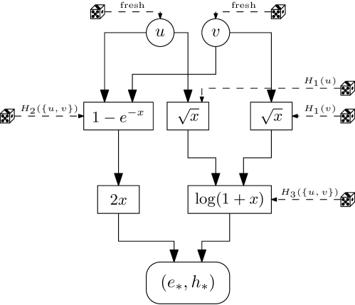
Figure 2: Circuit diagram for $G$-Edge-Sampler (Algorithm 4) with $G(a,b)=\log(1+\sqrt{a}+\sqrt{b})+2(1-e^{-(a+b)})$. Depicted are two of the input gates ($u$ and $v$), the unique output gate, and all gates related to the sampling of edge $\{u,v\}$. The dice symbol indicates the random seed $U\sim\mathrm{Uniform}(0,1)$ used by each $G$-gate, as well as the “fresh” exponential random variables $Y\sim\mathrm{Exp}(1)$ generated by the input gates for each update and each output wire. The “$2x$”-gate is a deterministic scalar gate with $\alpha=2$.

We illustrate how stochastic sampling circuits can be used to sample an edge from a graph with probability proportional to its weight. Let $H=([n],E)$ be a fixed graph and $\mathbf{x}\in\mathbb{R}_{+}^{n}$ be a vector of vertex weights subject to incremental updates. For a fixed edge-weight function $G:\mathbb{R}_{+}^{2}\to\mathbb{R}_{+}$, where the weight of $(u,v)$ is $G(\mathbf{x}(u),\mathbf{x}(v))$, we would like to select an edge $(u_{*},v_{*})$ with probability exactly $G(\mathbf{x}(u_{*}),\mathbf{x}(v_{*}))/\sum_{(u,v)\in E}G(\mathbf{x}(u),\mathbf{x}(v))$. Our running example is a symmetric weight function that exhibits summation, scalar multiplication, and a variety of $\mathcal{G}$-functions.

$$G(a,b)=\log(1+\sqrt{a}+\sqrt{b})+2(1-e^{-(a+b)}).$$

The stochastic sampling circuit corresponding to $G$ is depicted in Fig. 2. It uses the following level and hash functions.

• $\ell_{1}$, level function for $G_{1}(x)=\sqrt{x}$. See Example 3.

• $\ell_{2}$, level function for $G_{2}(x)=1-e^{-x}$. See Example 4.

• $\ell_{3}$, level function for $G_{3}(x)=\log(1+x)$. See Example 5.

• $H_{1}:V\to(0,1)$ uniformly at random.

• $H_{2},H_{3}:E\to(0,1)$ uniformly at random.

The implementation of this circuit as a $G$-Edge-Sampler is given in Algorithm 4. Note that since $G$ is symmetric, we can regard $H$ as an undirected graph and let Update$(v,\Delta)$ treat all edges incident to $v$ in the same way. If $G$ were not symmetric, the code for $G$-Edge-Sampler would have two for loops, one for outgoing edges $(v,u)\in E$, and one for incoming edges $(u,v)\in E$.

Algorithm 4 $G$-Edge-Sampler for $G(a,b)=\log(1+\sqrt{a}+\sqrt{b})+2(1-e^{-(a+b)})$

Specifications: $H=([n],E)$ is a fixed graph. The state is $(e_{*},h_{*})\in{[n]\choose 2}\cup\{\perp\}\times\mathbb{R}_{+}\cup\{\infty\}$, initially $(\perp,\infty)$. After processing a stream of updates, $\mathbb{P}(e_{*}=\{u_{*},v_{*}\})=G(\mathbf{x}(u_{*}),\mathbf{x}(v_{*}))/\sum_{\{u,v\}\in E}G(\mathbf{x}(u),\mathbf{x}(v))$.

1:procedure Update($v,\Delta$) $\triangleright$ $\mathbf{x}(v)\leftarrow\mathbf{x}(v)+\Delta$

2:     for each edge $\{u,v\}$ adjacent to $v$ do

3:         Generate fresh, independent $Y_{1},Y_{2}\sim\mathrm{Exp}(1)$

4:         $h\leftarrow\min\{\ell_{3}(\ell_{1}(Y_{1}/\Delta,H_{1}(v)),H_{3}(\{u,v\})),\,\ell_{2}(Y_{2}/\Delta,H_{2}(\{u,v\}))/2\}$

5:         if $h<h_{*}$ then

6:              $(e_{*},h_{*})\leftarrow(\{u,v\},h)$          

7:     end for

8:end procedure

6 Conclusion

In this paper we developed very simple sketches for perfect $G$-sampling using $O(\log n)$ bits and universal perfect $\mathcal{G}$-sampling using $O(\log^{2}n)$ bits. (See Remark 1 in Section 3 for a discussion of truly perfect implementations.) They were made possible by the explicit connection between the class $\mathcal{G}$ and the Laplace exponents of non-negative Lévy processes via the Lévy-Khintchine representation theorem (Theorem 3). To our knowledge this is the first explicit use of the Lévy-Khintchine theorem in algorithm design, though the class $\mathcal{G}$ was investigated without using this connection, by Cohen [3, 4, 5] and Cohen and Geri [6]. A natural question is whether $\mathcal{G}$ captures all functions that have minimal-size $O(\log n)$-bit perfect samplers.

Conjecture 1.

Suppose $\mathbf{x}\in\mathbb{R}_{+}^{n}$ is updated by an incremental stream. If there is an $O(\log n)$-bit perfect $G$-sampler in the random oracle model (i.e., an index $v\in[n]$ is sampled with probability $G(\mathbf{x}(v))/G(\mathbf{x})\pm 1/\text{poly}(n)$), then $G\in\mathcal{G}$.

Recall that $\mathcal{G}$ is in correspondence with non-negative, one-dimensional Lévy processes, which is just a small subset of all Lévy processes. It leaves out processes over $\mathbb{R}^{d}$, compound Poisson processes whose jump distribution includes positive and negative jumps, and $p$-stable processes for $p\in[1,2]$, among others. Exploring the connection between general Lévy processes, Lévy-Khintchine representation, and data sketches is a promising direction for future research.

Appendix A Sampling Without Replacement

We can take $k$ independent copies of the $G$-Sampler or ParetoSampler sketches to sample $k$ indices from the $(G(\mathbf{x}(v))/G(\mathbf{x}))_{v\in[n]}$ distribution with replacement. A small change to these algorithms will sample $k$ indices without replacement. See Cohen, Pagh, and Woodruff [7] for an extensive discussion of why WOR (without replacement) samplers are often more desirable in practice. The algorithm $(G,k)$-Sampler-WOR(Algorithm 5) samples $k$ (distinct) indices without replacement.

Algorithm 5 $(G,k)$-Sampler-WOR

Specifications: The state is a set $S\subset[n]\times\mathbb{R}_{+}$, initially empty. The function $k\textsf{-Min}(L)$ takes a list $L\subset[n]\times\mathbb{R}_{+}$, discards any $(v,h)\in L$ if there is a $(v,h^{\prime})\in L$ with $h^{\prime}<h$, then returns the $k$ elements with the smallest second coordinate.

1:procedure Update($v,\Delta$) $\triangleright$ $\mathbf{x}(v)\leftarrow\mathbf{x}(v)+\Delta$

2:     Generate fresh $Y\sim\mathrm{Exp}(1)$.

3:     $h\leftarrow\ell_{G}(Y/\Delta,H(v))$ $\triangleright$ $\ell_{G}$ is level function of $G$

4:     $S\leftarrow k\textsf{-Min}(S\cup\{(v,h)\})$

5:end procedure

In a similar fashion, one can define a sketch $k$-ParetoSampler-WOR analogous to $(G,k)$-Sampler-WOR, that maintains the minimum $k$-Pareto frontier, defined by discarding any tuple $(a,b,v)$ if there is another $(a^{\prime},b,v)$ with $a^{\prime}<a$, then retaining only those tuples that are dominated by at most $k-1$ other tuples.

Theorem 4.

Consider a stream a $\text{poly}(n)$ incremental updates to a vector $\mathbf{x}\in\mathbb{R}_{+}^{n}$. The $(G,k)$-Sampler-WOR occupies $2k$ words of memory, and can report an ordered tuple $(v_{*}^{1},\ldots,v_{*}^{k})\in[n]^{k}$ such that

$$\mathbb{P}((v_{*}^{1},\ldots,v_{*}^{k})=(v^{1},\ldots,v^{k}))=\prod_{i=1}^{k}\frac{G(\mathbf{x}(v^{i}))}{G(\mathbf{x})-\sum_{j=1}^{i-1}G(\mathbf{x}(v^{j}))}.$$ (3)

The $k$-ParetoSampler occupies $O(k\log n)$ words w.h.p. and for any $G\in\mathcal{G}$ at query time, can report a tuple $(v_{*}^{1},\ldots,v_{*}^{k})\in[n]^{k}$ distributed according to Eq. 3.

Proof.

The proof of Theorem 1 shows that $h_{v}\sim\mathrm{Exp}(G(\mathbf{x}(v)))$ and if $v_{*}^{1}$ minimizes $h_{v_{*}^{1}}$, that $h_{v_{*}^{1}}\sim\mathrm{Exp}(G(\mathbf{x}))$. It follows that $\mathbb{P}(v_{*}^{1}=v)=G(\mathbf{x}(v))/G(\mathbf{x})$. By the memoryless property of the exponential distribution, for any $v\neq v_{*}^{1},$ $h_{v}-h_{v_{*}^{1}}\sim\mathrm{Exp}(G(\mathbf{x}(v)))$, hence $h_{v_{*}^{2}}\sim\mathrm{Exp}(G(\mathbf{x})-G(\mathbf{x}(v_{*}^{1})))$ and $\mathbb{P}(v_{*}^{2}=v\mid v_{*}^{1},v\neq v_{*}^{1})=G(\mathbf{x}(v))/(G(\mathbf{x})-G(\mathbf{x}(v_{*}^{1})))$. The distribution of $v_{*}^{3},\ldots,v_{*}^{k}$ is analyzed in the same way.

By the 2D-monotonicity property, the $k$-Pareto frontier contains all the points that would be returned by $(G,k)$-Sampler-WOR, hence the output distribution of $k$-ParetoSampler-WOR is identical. The analysis of the space bound follows the same lines, except that $X_{i}$ is the indicator for the event that $h_{v_{i}}$ is among the $k$-smallest elements of $\{h_{v_{1}},\ldots,h_{v_{i}}\}$, so $\mathbb{E}(X_{i})=\min\{k/i,1\}$, $\mathbb{E}(|S|)<kH_{n}$, and by a Chernoff bound, $|S|=O(k\log n)$ with high probability. ∎

References

• [1] Alexandr Andoni, Robert Krauthgamer, and Krzysztof Onak. Streaming algorithms via precision sampling. In Proceedings 52nd Annual IEEE Symposium on Foundations of Computer Science (FOCS), pages 363–372, 2011.
• [2] Edith Cohen. Size-estimation framework with applications to transitive closure and reachability. Journal of Computer and System Sciences, 55(3):441–453, 1997.
• [3] Edith Cohen. HyperLogLog hyperextended: Sketches for concave sublinear frequency statistics. In Proceedings 23rd ACM SIGKDD International Conference on Knowledge Discovery and Data Mining (KDD), pages 105–114, 2017.
• [4] Edith Cohen. Stream sampling framework and application for frequency cap statistics. ACM Trans. Algorithms, 14(4):52:1–52:40, 2018.
• [5] Edith Cohen. Sampling big ideas in query optimization. In Proceedings 42nd ACM SIGMOD-SIGACT-SIGAI Symposium on Principles of Database Systems (PODS), pages 361–371, 2023.
• [6] Edith Cohen and Ofir Geri. Sampling sketches for concave sublinear functions of frequencies. In Proceedings of the Annual Conference on Neural Information Processing Systems (NeurIPS), pages 1361–1371, 2019.
• [7] Edith Cohen, Rasmus Pagh, and David P. Woodruff. WOR and $p$’s: Sketches for $\ell_{p}$-sampling without replacement. In Proceedings of the Annual Conference on Neural Information Processing Systems (NeurIPS), 2020.
• [8] Rajesh Jayaram. Sketching and Sampling Algorithms for High-Dimensional Data. PhD thesis, Carnegie Mellon University Pittsburgh, PA, 2021.
• [9] Rajesh Jayaram and David P. Woodruff. Perfect $L_{p}$ sampling in a data stream. SIAM J. Comput., 50(2):382–439, 2021.
• [10] Rajesh Jayaram, David P. Woodruff, and Samson Zhou. Truly perfect samplers for data streams and sliding windows. In Proceedings 41st ACM SIGMOD-SIGACT-SIGART Symposium on Principles of Database Systems (PODS), pages 29–40, 2022.
• [11] Hossein Jowhari, Mert Saǧlam, and Gábor Tardos. Tight bounds for $L_{p}$ samplers, finding duplicates in streams, and related problems. In Proceedings 30th ACM SIGMOD-SIGACT-SIGART Symposium on Principles of Database Systems (PODS), pages 49–58, 2011.
• [12] Morteza Monemizadeh and David P. Woodruff. 1-pass relative-error $L_{p}$-sampling with applications. In Proceedings 21st Annual ACM-SIAM Symposium on Discrete Algorithms (SODA), pages 1143–1160, 2010.
• [13] Karol A. Penson and Katarzyna Górska. Exact and explicit probability densities for one-sided Lévy stable distributions. Physical Review Letters, 105(21):210604.1–210604.4, 2010.
• [14] Ken-Iti Sato. Lévy processes and infinitely divisible distributions, volume 68 of Cambridge Studies in Advanced Mathematics. Cambridge University Press, 1999.
• [15] Jeffrey S. Vitter. Random sampling with a reservoir. ACM Transactions on Mathematical Software (TOMS), 11(1):37–57, 1985.