Multiple Interacting Photonic Modes in Strongly Coupled Organic Microcavities

Abstract

Room temperature cavity quantum electrodynamics with molecular materials in optical cavities offers exciting prospects for controlling electronic, nuclear and photonic degrees of freedom for applications in physics, chemistry and materials science. However, achieving strong coupling with molecular ensembles typically requires high molecular densities and substantial electromagnetic field confinement. These conditions usually involve a significant degree of molecular disorder and a highly structured photonic density of states. It remains unclear to what extent these additional complexities modify the usual physical picture of strong coupling developed for atoms and inorganic semiconductors. Using a microscopic quantum description of molecular ensembles in realistic multimode optical resonators, we show that the emergence of a vacuum Rabi splitting in linear spectroscopy is a necessary but not sufficient metric of coherent admixing between light and matter. In low finesse multi-mode situations we find that molecular dipoles can be partially hybridised with photonic dissipation channels associated with off-resonant cavity modes. These vacuum-induced dissipative processes ultimately limit the extent of light-matter coherence that the system can sustain.

I Introduction

Strong coupling between a large ensemble of molecules and an optical cavity mode is still a rapidly evolving field, despite being more than 25 years old Lidzey_PRL_1999_82_3316 . In strong coupling hybridization takes place between a molecular resonance and a cavity mode to yield two new polariton modes (states), modes that inherit characteristics of both light and matter. Two broad schemes have attracted the most attention: exciton-polaritons, where an excitonic molecular resonance is coupled to a cavity mode, and vibrational-polaritons, where a molecular vibrational mode is coupled to a cavity mode. Despite considerable progress, an underlying theoretical framework has yet to be established that provides a coherent picture of strong coupling phenomena to be given. Here we identify and explore one largely ignored ingredient, the multiple photonic modes nature of the cavities typically employed.

One of the main attractions of molecular strong coupling is that the key phenomenon, that of an anti-crossing between a molecular resonance and a photonic mode, can be explained with a very simple model based on two coupled oscillators, one oscillator representing the molecular system (a large number of identical molecules are taken to behave as though they are a single oscillator) the other representing a single photonic (cavity) resonance. This simple picture is a powerful one, but can do little to capture a wealth of important features, including dark states, disorder, and especially material behaviour such as reactivity. It is for this reason that so much effort has been devoted to developing a wider theoretical framework. Significant progress has been made by building more realistic models of the molecular systems involved, as reviewed recently Herrera2020perspective ; Sanchez2022 ; Mandal2023 .

Much of the theoretical work on strong coupling in the past few years has been devoted to incorporating the complexities that arise when including more realistic numbers of molecules (typically models have $<10^{3}$, whilst in experiments there may be $>10^{8}$) Bhuyan_AOM_2023_12_2301383 , and the presence of disorder Khazanov_ChemSocRev_2023_4_041305 . Various approaches have been explored, examples include: employing a Holstein-Tavis-Cummings (HTC) model Spano2015 ; Cwik2014 ; Herrera2016 ; Herrera_PRL_2017_118_223601 together with a Markovian Herrera2017-PRA ; delPino2018 approach for the dissipative dynamics of organic polaritons; ab-initio studies RuggenthalerP_PRA_2014_90_012508 ; Flick_PNAS_2017_114_3026 ; and multiscale molecular dynamics simulations Luk_JCTC_2017_13_4324 . Whilst these theoretical approaches strive to include more realistic models for the molecular ensembles involved, little if any attention appears to have been directed towards including photonic complexities.

It was recognised early on that the dispersion of the photon (cavity) modes was important Agranovich_PRB_2003_67_085311 , and recent studies have focused on dispersion in connection with energy transport Ribeiro2022 . Whilst dispersion of a given photon mode is indeed important in several processes of interest such as condensation Keeling2020 and lasing Arnardottir2020 , the fact that most cavities that are currently employed in experiments support several discrete cavity modes George_PRL_2016_117_153601 , has been largely overlooked. An unwritten assumption seems to have been that if the spacing between cavity modes (the free-spectral range) is ‘sufficient’, then the presence of many (rather than one) photonic modes can be ignored as having minimal influence on the polariton properties. Indeed, this presumed minimal effect has led to the use of ‘off-resonance’ modes being employed to monitor changes in the constituents within a cavity Thomas_JCP_2024_160_204303 . Here we show explicitly that the presence of multiple photonic modes can have a significant effect on the strong coupling process. Recently the importance of this effect has been recognized in other physical implementations of cavity QED, e.g. artificial atoms in superconducting resonators Sundaresan_PRX_2015_5_021035 . The model elucidated here is an expanded version of an outline we recently presented to explain polariton-mediated photoluminescence in low finesse cavities menghrajani2024 . Before looking at our multi-mode framework in detail, let us briefly mention some of the prior work on multimode cavities.

Multi-mode cavities have been employed in a large number of experiments, both for excitonic strong coupling (see for example Coles_APL_2014_104_191108 ; Georgiou_JCP_2021_154_124309 ; Godsi_JCP_2023_159_134307 ) and vibrational strong coupling (see for example Shalabney_NatComm_2015_6_5981 ; Simpkins_ACSPhotonics_2015_2_1460 ; George_PRL_2016_117_153601 ; Hertzog_ChemPhotChem_2020_4_612 ), but the implications of there being more than one mode have in general only involved considering the presence of single couplings, i.e. coupling between the molecular mode and each of the photonic modes. For example, when more than one photonic mode is involved then one has to take care about mode assignment due to the overlap (in energy) between different polariton bands George_PRL_2016_117_153601 . However, as we show below, one also needs to consider how the couplings between different photonic modes alters the overall picture. One of our major findings is that such couplings can limit the extent of light-matter mixing, and may thus limit the coherence of polaritons, with possible consequences for a variety of phenomena such as photoluminescence menghrajani2024 and polariton transport Balasubrahmaniyam_NatMat_2023_22_338 .

Figure 1 provides a schematic overview of our model. In molecular strong coupling an excitonic resonance is usually considered to interact with a single cavity mode, depicted in panel (a). Although other cavity modes might be present, they do not spectrally overlap with the cavity mode being considered, they are too far detuned. However, when the finesse is low, adjacent cavity modes may overlap and may thus couple to each other and to the excitonic resonance, see panel (b). In this situation the strong coupling is no longer single mode, the exciton resonance now being ‘spread’ over more than one cavity mode. The work reported here is the result of an investigation to explore the consequences of this ‘spreading’.

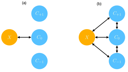
Figure 1: Schematic: Left, panel (a). Although several cavity modes are present ($C_{-1}$, $C_{0}$ and $C_{+1}$), our excitonic molecular resonance $X$ interacts with a single discrete on-resonance cavity mode, $C_{0}$. Right, panel (b). Now the finesse is low and there is spectral overlap between adjacent photonic (cavity) modes. The excitonic resonance interacts directly with the various cavity modes, and there is also direct interaction between adjacent photonic modes. The consequence is that the excitonic resonances is now ‘spread out’ over more than one cavity mode.

II Multi-Mode Theory of Organic Microcavities

Our aim is to build a model for molecular optical cavities that correspond to an ensemble of $N$ electronic dipole emitters coupled to the full set of resonant optical modes supported by a (planar) cavity structure. In what follows we restrict the discussion to molecular dipoles with negligible Huang-Rhys factor Hestand2018 , such that their emission properties are accurately described by considering only the vibration-less ground ($S_{0}\equiv g$) and first excited ($S_{1}\equiv e$) electronic states (see Refs. Hobson2002 ; Wang2019singlemolecule for examples). The system is described by a multimode Tavis-Cummings Hamiltonian of the form ($\hbar\equiv 1$ throughout),

$$\hat{\mathcal{H}}=\sum_{q}\omega_{q}\hat{a}^{\dagger}_{q}\hat{a}_{q}+\sum_{i=1}^{N}\omega_{i}\hat{\sigma}_{i}^{+}\hat{\sigma}_{i}^{-}+\sum_{q}\sum_{i=1}^{N}\,g_{iq}\hat{\sigma}_{i}^{+}\,\hat{a}_{q}+g_{iq}^{*}\,\hat{\sigma}_{i}^{-}\hat{a}_{q}^{\dagger},$$ (1)

where $q=\{\mathbf{q}_{\parallel},q_{\perp}\}$ is generally a composite photonic mode index describing the continuous in-plane component of the wavevector $\mathbf{q}_{\parallel}$ and the discrete transverse component $q_{\perp}$ of confined electromagnetic modes in planar cavities Skolnick1998 . The local dipole transition operators between ground $\ket{g_{i}}$ and excited state $\ket{e_{i}}$ are defined as $\hat{\sigma}_{i}^{-}=\ket{g_{i}}\bra{e_{i}}$ for emission and $\hat{\sigma}_{i}^{+}=(\hat{\sigma}_{i}^{-})^{\dagger}$ for absorption. The electronic transition frequency $\omega_{i}$ is in general inhomogeneously distributed, although there are examples of organic emitters with negligible inhomogeneous broadening Wang2019 . Bosonic cavity field operators are $\hat{a}_{q}$, and the local mode-dependent Rabi couplings are denoted by $g_{iq}$.

Ideal planar cavities of length $L$ have photon dispersion $\omega_{q}=(c/n_{\rm d})({q_{\parallel}^{2}+q_{\perp}^{2}(m)})^{1/2}$, where $q_{\perp}(m)=m\pi/2L$, with $m\geq 1$ an integer, which determines the discrete set of allowed cavity mode energies at normal incidence ($q_{\parallel}=0$); $c$ is the speed of light and $n_{d}$ the (real) dielectric constant of the intracavity medium. The mode dispersion with respect to the in-plane wavevector $\mathbf{q}_{\parallel}$ determines the propagation properties of the normal modes of the coupled system, which for strong light-matter coupling correspond to exciton-polaritons Lidzey1998 ; Barnes1998 ; kena-cohen2008 , and the free spectral range (FSR) between adjacent modes $\Delta_{q}\equiv\omega_{q+1}-\omega_{q}$, is controlled at normal incidence ($q_{\parallel}=0$) by the cavity length as $\Delta=c\pi/2n_{d}L$. Throughout this work, we neglect dispersion and only study system properties at $q_{\parallel}=0$.

The explicit multimode structure of Eq. (1) generalizes early approaches that simplify the mode structure of the microcavity to having a single dispersionless mode $\hat{a}$ Herrera2017-review , or a dispersive mode $\hat{a}_{q_{\parallel}}$ in a cavity with infinite FSR. Such simplifications are often introduced as a necessity in favour of capturing relevant aspects of complexity of the internal degrees of freedom of the molecular dipole emitters, such as high-frequency vibrations Cwik2014 ; Spano2015 ; Herrera2016 ; Herrera2017-PRA ; Herrera_PRL_2017_118_223601 ; Spano2020 , electron tunnelling Hagenmuller2017 , or the role of static disorder in establishing quantum transport regimes Engelhardt2023 ; Chavez2021 ; Ribeiro2022 . Single-mode or single-branch theories are intrinsically limited with respect to their ability to describe the influence of multiple transverse photonic modes in realistic organic microcavites with finite FSR, $\Delta$, as the value of $\Delta$ is not much larger than the frequency separation between lower and upper polaritons, i.e. the Rabi splitting $\Omega_{R}$. For some systems $\Delta$ is even smaller than $\Omega_{R}$ Kena-Cohen2013 .

III Microcavities as Open Quantum Systems

We model the organic microcavity microscopically as an open quantum system described by a Lindblad quantum master equation for the light-matter reduced density matrix $\hat{\rho}$, given by Breuer-book ,

$$\frac{d}{dt}\hat{\rho} = -i[\hat{\mathcal{H}},\hat{\rho}]+\sum_{q}\frac{\kappa_{q}}{2}\left(2\hat{a}_{q}\hat{\rho}\hat{a}_{q}^{\dagger}-\hat{a}_{q}^{\dagger}\hat{a}_{q}\hat{\rho}-\hat{\rho}\hat{a}_{q}^{\dagger}\hat{a}_{q}\right)$$ (2)

$$+\sum_{i}\frac{\gamma_{i}}{2}\left(2\hat{\sigma}^{-}_{i}\hat{\rho}\hat{\sigma}^{+}_{i}-\hat{\sigma}_{i}^{+}\hat{\sigma}^{-}_{i}\hat{\rho}-\hat{\rho}\hat{\sigma}_{i}^{+}\hat{\sigma}_{i}^{-}\right),$$

where $\kappa_{q}$ is the bare radiative decay rate of the $q$-th cavity mode and $\gamma_{i}$ the bare spontaneous decay rate of the $i$-th electronic dipole excitation, which includes radiative and non-radiative contributions. For simplicity, we ignored cross-terms that could dissipatively couple different cavity modes or different molecules, under the assumption that direct diagonal relaxation channels are much faster.

The Lindblad master equation is the basis for deriving effective non-unitary propagators that unravel the state evolution as an ensemble of wavefunction trajectories Molmer:93 . For the light-matter state ansatz,

$$\ket{\Psi(t)}\approx\sqrt{1-\xi(t)}\ket{\psi^{(0)}(t)}+\sqrt{\xi(t)}\ket{\psi^{(1)}(t)},$$ (3)

with $\xi\ll 1$, as is relevant for weakly excited microcavities, we can ignore stochastic quantum jumps coming from the recycling terms of the Lindblad equation Herrera2017-PRA , and account for dissipation as an exponential decay of the excited state population. This is equivalent to rewriting Eq. (2) as,

$$\frac{d}{dt}\hat{\rho}=-i[\hat{\mathcal{H}}_{\rm eff},\hat{\rho}]+\mathcal{L}_{1}[\hat{\rho}],$$ (4)

with an effective non-Hermitian Hamiltonian,

$$\hat{\mathcal{H}}_{\rm eff}=\hat{\mathcal{H}}-\frac{i}{2}\sum_{q}\kappa_{q}\hat{a}^{\dagger}_{q}\hat{a}_{q}-\frac{i}{2}\sum_{i}\gamma_{i}\hat{\sigma}_{i}^{+}\hat{\sigma}_{i}^{-}.$$ (5)

As mentioned above, we ignore the recycling terms $\mathcal{L}_{1}[\hat{\rho}]\equiv\sum_{q}\kappa_{q}\hat{a}_{q}\hat{\rho}\hat{a}_{q}^{\dagger}+\sum_{i}\gamma_{i}\hat{\sigma}^{-}_{i}\hat{\rho}\hat{\sigma}^{+}_{i}$. This simplified approach to the open system dynamics effectively reduces the problem to one of solving a non-Hermitian Schrodinger equation with the effective Hamiltonian $\hat{\mathcal{H}}_{\rm eff}$.

Since the ground state $\ket{\psi^{(0)}}$ has no electronic or photonic excitations, the dynamics of polaritons is fully determined by the excited electron-photon wavefunction

$$\ket{\psi^{(1)}}=\sum_{i}c_{i}^{(0)}\ket{e_{i}}\ket{\{0_{q}\}}+\sum_{q}\,c_{q}^{(1)}\ket{g_{1}g_{2},\ldots,g_{N}}\ket{1_{q}},$$ (6)

where $\ket{\{0_{q}\}}$ is the multi-mode cavity vacuum, $\ket{e_{i}}$ describes a single excitation in the $i$-th molecule with all other dipoles in the ground state. $\ket{1_{q}}$ describes a single photon in the $q$-th transverse mode, all other modes being empty.

IV Strong Coupling in High-Finesse Cavities

Consider $N$ molecular dipoles coupled near resonantly with a $q=0$ mode of frequency $\omega_{0}$ and decay rate $\kappa_{0}$. Higher and lower order cavity modes are detuned from the central frequency by $\Delta_{q}=\omega_{q}-\omega_{0}$, with $\Delta_{q}>0$ for higher-order and $\Delta_{q}<0$ for lower-order modes. They also have bandwidths that in general differ from $q=0$ by $\Delta\kappa_{q}=\kappa_{q}-\kappa_{0}$. In the large finesse limit, $|\Delta_{q}|\gg\Omega_{0}$, with $\Omega_{0}=\sqrt{N}g_{0}$ being the single-mode Rabi coupling strength for a homogeneous molecular ensemble, dipole excitations cannot exchange energy effectively with higher and lower order cavity modes. (Note, the single mode Rabi splitting $\Omega^{SM}_{R}$ is related to the single mode Rabi coupling $\Omega_{0}$ as $\Omega^{SM}_{R}$ = 2$\Omega_{0}$.) Consequently, light-matter hybridization leading to polariton formation only occurs in the vicinity of the near-resonant $q=0$ mode, see panel (a) of figure 1. However, far de-tuned modes do have an effect via second order (two photon) processes, something we look at next.

Far-detuned higher and lower-order modes evolve on a timescale of $1/\Delta_{q}$, which is much faster than the Rabi oscillation period $\tau_{R}\sim 1/\Omega_{0}$ between the near-resonant mode and molecular excitations. These fast-oscillating mode variables thus adiabatically adjust to the dynamics of the near-resonant manifold, which affects the process of polariton formation around $q=0$. This can be understood as the emergence of Raman-type processes in which molecules absorb and re-emit virtual photons from higher and lower-order modes. These two-photon processes result in a change to the energetics; a single-molecule frequency shift of the form,

$$\Gamma_{j}^{{}^{\prime\prime}}=-\sum_{q\neq 0}|g_{jq}|^{2}\frac{\Delta_{q}}{\Delta_{q}^{2}+(\Delta\kappa_{q}/2)^{2}},$$ (7)

and an effective inter-molecular coupling with interaction energy given by,

$$J_{ij}^{\prime\prime}=-\sum_{q\neq 0}g_{iq}^{*}g_{jq}\frac{\Delta_{q}/2}{\Delta_{q}^{2}+(\Delta\kappa_{q}/2)^{2}}.$$ (8)

The sign of the contributions per mode in these expressions is different for lower-order modes (blue shift and repulsive interaction) and higher-order modes (red shift and attractive interactions). In general, $J_{ij}^{\prime\prime}$ is a complex-valued quantity depending on the relative phase of the Rabi frequency at the location of the two dipoles.

Cavity-induced frequency shifts and inter-dipole interactions induced by far-detuned modes are well-known from atomic physics Raimond2001 and have been used for quantum state preparation in high-quality resonators Leroux2010 . Organic microcavities are qualitatively different from atomic cavities in that their quality factors are much lower, typically $Q\sim 1-10$, and changes in bandwidth $\kappa_{q}$ with mode order can be large. This is particularly true for modes close to the region where absorption of metal mirrors cannot be neglected Thomas_AdvMat_2024_36_2309393 . Therefore, in addition to the changes in frequency and interaction energy discussed above, the dispersive interaction of molecular dipoles with far-detuned lossy modes also changes the single-molecule dipole decay rates by,

$$\Gamma_{j}^{\prime}=-\sum_{q\neq 0}|g_{jq}|^{2}\frac{\Delta\kappa_{q}/2}{\Delta_{q}^{2}+(\Delta\kappa_{q}/2)^{2}},$$ (9)

and establishes the two-body loss rate,

$$J_{ij}^{\prime}=-\sum_{q\neq 0}g_{iq}^{*}g_{jq}\frac{\Delta\kappa_{q}/2}{\Delta_{q}^{2}+(\Delta\kappa_{q}/2)^{2}}.$$ (10)

These are again signed quantities summed over all available modes, whose contribution depends on the relative bandwidths $\Delta\kappa_{q}$. If all relevant modes have bandwidths $\kappa_{q}$ equal to the resonant ($q=0$) mode, then $\Delta\kappa_{q}\approx 0$ and no second-order corrections to the decay rates are expected. The bandwidth mismatch of sub-wavelength cavities thus introduces a phenomenology that is not present in other cavity QED systems, we discuss one key aspect next.

The dispersive relaxation channels discussed above involving material degrees of freedom could, in principle, alter the ability to establish strong coupling with the central $q=0$ mode. To assess this, consider a simplified homogeneous scenario in which all dipoles are identical (Dicke regime) and the polariton wavefunction in Eq. (6) reduces to,

$$\ket{\psi^{(1)}}=\beta\ket{X}\ket{0}+\alpha\ket{g_{1}g_{2},\ldots,g_{N}}\ket{1},$$ (11)

where $\ket{X}=\sum_{j}\ket{e_{j}}/\sqrt{N}$ is the fully-symmetric excitonic state and the Fock states $\{\ket{0},\ket{1}\}$ refer to the central $q=0$ mode. The dynamics of the state vector $\mathbf{x}=[\alpha,\beta]^{\rm T}$ can be written as $\dot{\mathbf{x}}=-iM\mathbf{x}$, where,

$$M=\left(\begin{array}[]{cc}0&\Omega_{0}\\ \Omega_{0}&-\delta_{N}-i\Delta\Gamma_{N}\end{array}\right),$$ (12)

is the dynamical matrix whose complex eigenvalues $\lambda=E+i\Gamma/2$ give the polariton energies, $E$, and bandwidths, $\Gamma$. $\Omega_{0}=\sqrt{N}g_{0}$ is the Rabi coupling strength. The effective detuning $\delta_{N}$ and bandwidth mismatch $\Delta\Gamma_{N}$ can be written as

$$\delta_{N} = \delta_{0}-\Gamma{{}^{\prime\prime}}-NJ{{}^{\prime\prime}}$$ (13)

$$\Delta\Gamma_{N} = -\Delta\gamma/2+\Gamma^{\prime}+NJ{{}^{\prime}},$$ (14)

where $\delta_{0}=\omega_{0}-\omega_{e}$ and $\Delta\gamma=\kappa_{0}-\gamma$ are the bare detuning and bandwidth mismatch between the $q=0$ mode and the dipole resonance. The one-body and two-body energy shifts $\Gamma^{\prime\prime}$ and $NJ^{\prime\prime}$ contribute to the detuning of the $q=0$ mode from the molecular resonance. The one- and two-body decay rates $\Gamma^{\prime}$ and $NJ^{\prime}$ contribute to the bandwidth mismatch. The microscopic derivation of Eq. (12) starting from Eq. (5) is given in the appendix.

The real part of the eigenvalues of $M$ give the lower and upper polariton frequencies, $E_{\rm LP}$ and $E_{\rm UP}$, respectively. The Rabi splitting $\Omega_{R}\equiv E_{\rm UP}-E_{\rm LP}$ can thus be written as

$$\Omega_{R}={\rm Re}\sqrt{(NJ^{\prime\prime}-\delta_{0}-i(NJ^{\prime}-\Delta\gamma/2))^{2}+4\Omega_{0}^{2}},$$ (15)

where $\Gamma^{\prime}$ and $\Gamma^{\prime\prime}$ are neglected in the thermodynamic limit . Equation (15) gives the usual strong coupling result $\Omega_{R}=2\Omega_{0}$ for infinite finesse, $\Delta_{q}\rightarrow\infty$ and finite $N$, since $NJ^{\prime}\sim 1/\Delta_{q}^{2}$ and $NJ^{\prime\prime}\sim 1/\Delta_{q}$.

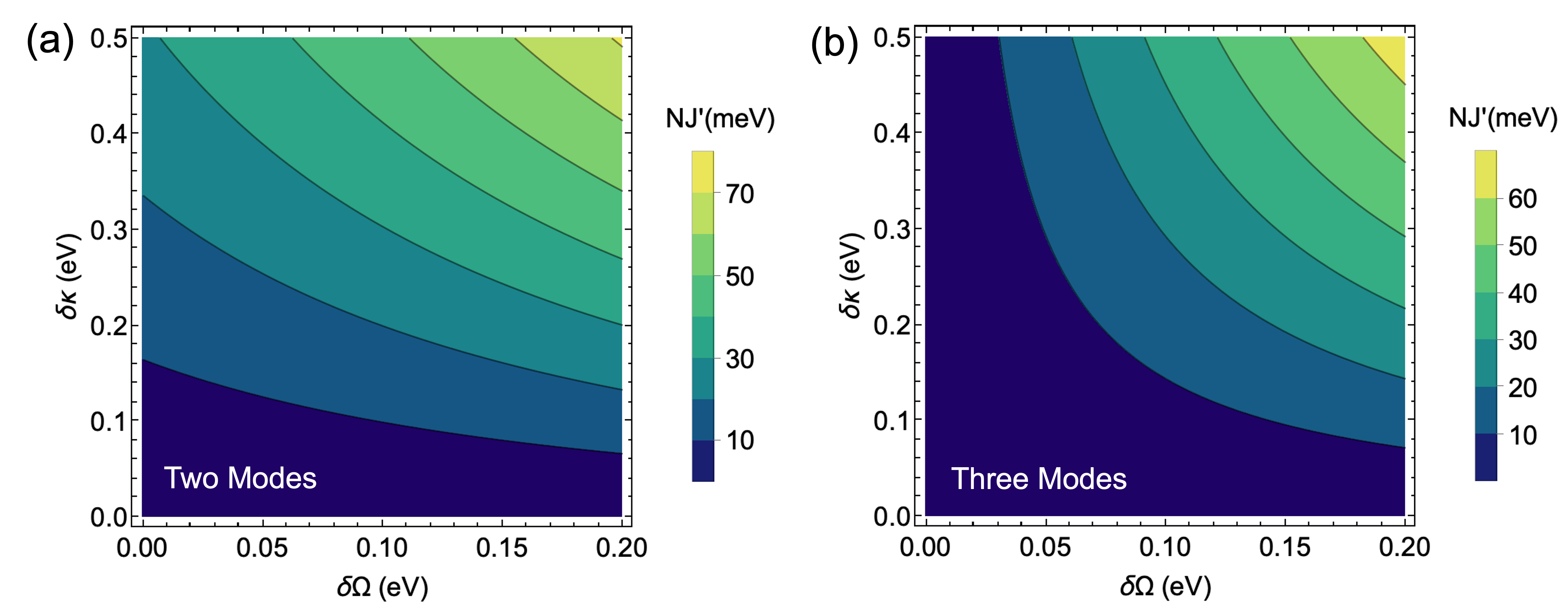
Figure 2: Modified polariton decay in high finesse cavities: Two-body contribution to the polariton decay rate $NJ^{\prime}$, as a function of the change in Rabi coupling $\delta\Omega$ and change in bandwidth $\delta\kappa$ relative to a reference $q=0$ strongly coupled resonant mode for two cases; (a) two-mode cavity where $q=0$ is the lowest order mode; (b) three-mode cavity with one lower and one higher-order mode. We use $\Omega_{0}=0.35$ eV and $\Delta=1.0$ eV.

To estimate the magnitude of $NJ^{\prime}$ for typical high-finesse cavities ($|\Delta_{q}|>\Omega_{R}$), consider a model three-mode cavity with a central $q=0$ mode at $\omega_{0}$, a lower-order mode ($q=-1$) detuned from $q=0$ by $\Delta_{-1}=-\Delta$ and a higher-order mode ($q=+1$) detuned by $\Delta_{+1}=\Delta$, with $\Delta>0$. The mode-dependent decay rates are $\{\kappa_{-},\kappa_{0},\kappa_{+}\}$, respectively. Without losing generality, we assume linear scaling of the bandwidth with mode order, i.e., $\kappa_{q}=\kappa_{0}+q\,\zeta$ with positive $\zeta$ for increasing bandwidth and negative otherwise. We also allow the Rabi coupling strength to depend on mode order as $\Omega_{\pm 1}\equiv\sqrt{N}g_{\pm 1}$, for collective coupling of dipoles to $q=\pm 1$ cavity modes. From Eq. (10), the two-body rate can be written as,

$$NJ{{}^{\prime}}=\left(\Omega_{-1}^{2}-\Omega_{+1}^{2}\right)\frac{\zeta/2}{{\Delta}^{2}+\zeta^{2}/4}\approx\frac{\zeta f\,\Omega_{0}^{2}}{{\Delta}^{2}+\zeta^{2}/4},$$ (16)

where in the second equality we used $\Omega_{\pm 1}=\Omega_{0}(1\pm f)$ with $|f|<1$. This contribution to the polariton decay can either increase or decrease the bandwidth of LP and UP resonances around the $q=0$ mode, depending on the sign of $\zeta f$.

Figure 2 shows the magnitude of $NJ^{\prime}$ from Eq. (16) as a function of the variation in Rabi coupling per mode $\delta\Omega=f\Omega_{0}$ and the variation in bandwidth $\delta\kappa=\zeta$, estimated for a system with $\Omega_{0}=0.35$ eV and FSR $\Delta=1.0$ eV. We consider a two-mode cavity (panel a), where $q=0$ is the lowest-order mode ($\Omega_{-1}=0$) and modes beyond $q=1$ are ignored, as well as the three-mode scenario (panel b). In general, the magnitude of $NJ^{\prime}$ is smaller than $k_{\rm B}T\approx 26\,{\rm meV}$ for multi-mode microcavities with relatively weak mode-dependence of the Rabi coupling and photon bandwidth ($\delta\Omega\sim\delta\kappa\sim 10^{-2}$ eV menghrajani2024 )), but the analysis above is general and larger polariton bandwitdh modifications could be expected for other high finesse photonic structures with greater cavity bandwidths and for coupling variations with mode order.

In summary, the presence of far off-resonance cavity modes can introduce adiabatic corrections to the Rabi splitting $\Omega_{R}$ established in strong coupling. Such corrections originate from coherent and incoherent two-photon Raman-type processes in which dipoles scatter virtual photons from far-detuned higher and lower-order modes, primarily leading to changes in the dipole bandwidth (Fig. 2). Since adiabatic corrections to $\Omega_{R}$ scale as $(\Omega_{0}/\Delta)^{2}$, it can be difficult to measure their contribution in typical high finesse Fabry-Perot microcavities ($\mathcal{F}\equiv\Delta/\kappa_{0}\gtrsim 10$, $\Omega_{0}/\Delta\lesssim 0.1$).

V Strong Coupling in Low-Finesse Cavities

The adiabatic elimination procedure in the previous Section is strictly valid for $\Omega_{R}/\Delta\ll 1$ and breaks down if the Rabi splitting is not much smaller than the FSR, even when the bare cavity finesse is nominally high ($\mathcal{F}\geq 10$).

For microcavities with lower finesse, there is no significant separation of scales between $\kappa$, $\gamma$, $\Omega_{0}$ and $\Delta$, although typically $\kappa\sim\gamma<\Omega_{0}<\Delta$ in strong coupling menghrajani2024 . For the light-matter system discussed above, with $N$ identical dipoles at $\omega_{e}$ resonant with a reference $q=0$ cavity mode at $\omega_{0}$, having Rabi coupling strength $\Omega_{0}$, the frequency separations $\Delta_{\pm 1}$ of adjacent higher-order and lower-order modes ($q\pm 1$) are comparable with the bare Rabi couplings $\Omega_{\pm 1}$ to those modes and thus the direct coupling of dipoles to neighbouring modes needs to be considered.

For the homogeneous dipole ensemble, the simplest extension of the light-matter state vector includes the next-order modes $q=\pm 1$, i.e., $\mathbf{x}=[\alpha_{-1},\alpha_{0},\alpha_{+1},\beta]^{\rm T}$, where $\alpha_{q}$ is the photon amplitude in the $q$-th mode. The dynamical matrix for this (3+1) system can be written as,

$$M=\left(\begin{array}[]{cccc}d_{-1}&0&0&e_{-1}\\ 0&0&0&e_{0}\\ 0&0&d_{+1}&e_{+1}\\ e_{-1}&e_{0}&e_{+1}&p\\ \end{array}\right),$$ (17)

where we used the simplified notation $d_{q}=\Delta_{q}-i\Delta\kappa_{q}/2$, $e_{q}=\Omega_{q}$ and $p=-\delta+i\Delta\gamma/2$. From the eigenvalues of $M$, $\lambda=E+i\Gamma/2$, the coupled energies $E$ and decay rates $\Gamma$ are obtained. In general, $\lambda$ is a root of the polynomial,

$$\Phi(\lambda)\equiv p-\lambda+\frac{e_{0}^{2}}{\lambda}-\frac{e_{-1}^{2}}{d_{-1}-\lambda}-\frac{e_{+1}^{2}}{d_{+1}-\lambda},$$ (18)

which for $\Omega_{\pm 1}=0$ gives the quadratic eigenvalue equation,

$$\lambda(\delta-i\Delta\gamma/2-\lambda)-\Omega_{0}^{2}=0,$$ (19)

that is often used to derive conditions for strong coupling in the single-mode picture. In particular, for resonant bandwidth-matched light-matter interaction with the $q=0$ mode ($\delta=0$, $\gamma=\kappa$), Eq. (19) gives the LP and UP frequencies $E_{\pm}=\pm\Omega_{0}$ ($\Omega_{R}=2\Omega_{0}$) with decay rates $\Gamma_{\pm}=\kappa$ .

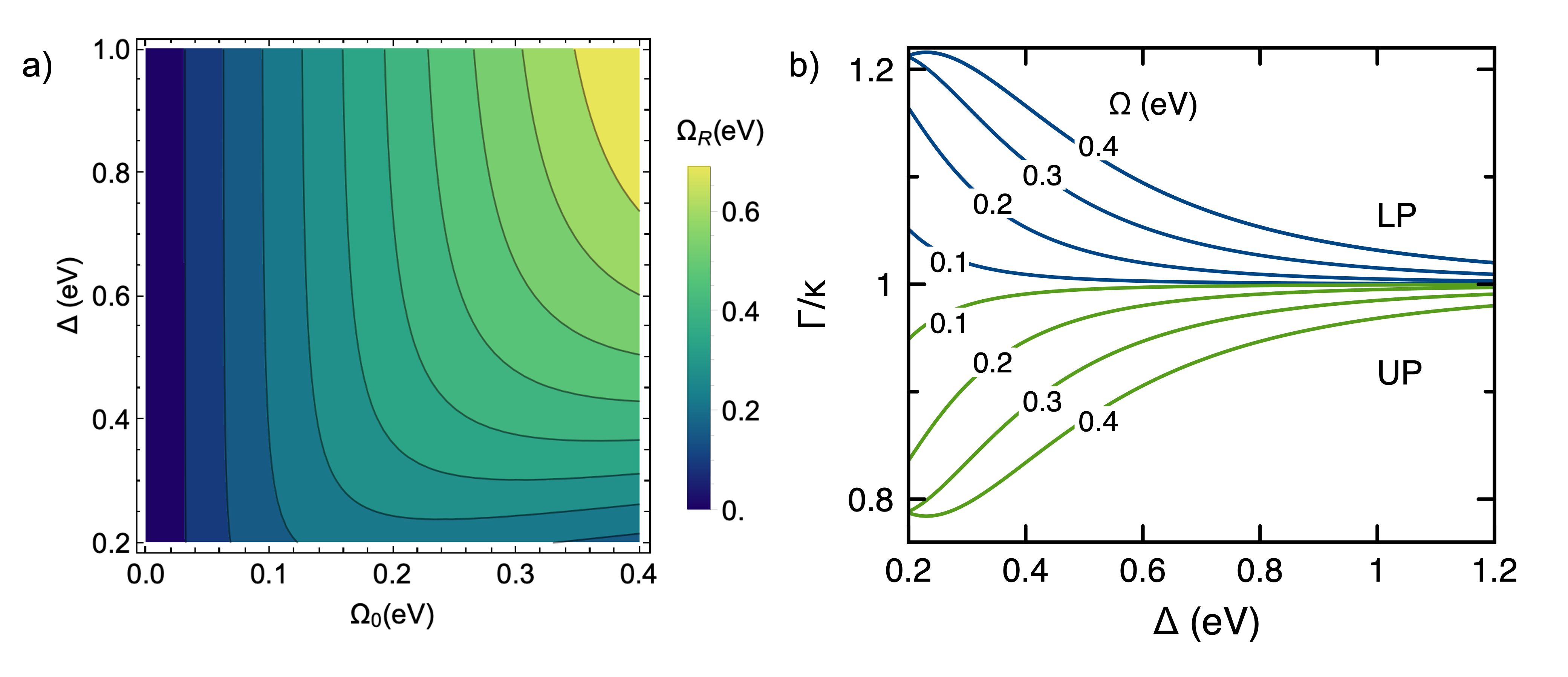
Figure 3: Modified Rabi splitting and bandwidth in low finesse cavities: (a) Rabi splitting $\Omega_{R}$ as function of the bare Rabi coupling $\Omega_{0}$ and free-spectral range $\Delta$ for a three-mode cavity ($q=\{0,\pm 1\}$) with the central mode on exact resonant with the dipole transition; (b) Decay rates $\Gamma$ of the Lower polariton (LP, blue lines) and upper polariton (UP, green lines) in units of $\kappa$, as functions of $\Delta$ for different values of the bare Rabi couping $\Omega_{0}$, for a linear variation of the mode bandwidths $\kappa_{q}=\kappa_{0}+q\zeta$. We use $\delta=0$, $\gamma=\kappa=0.1\,{\rm eV}$ and $\zeta=-0.1$ eV. -mode cavity with one lower and one higher-order mode. We use $\Omega_{0}=\Omega_{\pm 1}=0.35$ eV, $\kappa=\gamma=0.15\,{\rm eV}$, $\zeta=-0.1\,{\rm eV}$.

Direct coupling of dipoles to the $q=\pm 1$ modes modifies the LP and UP energies and bandwidths. In the appendix we derive a general expression for the lowest-order corrections to the energies and bandwidths of the single-mode polariton problem, due to the presence of neighbouring cavity modes. These corrections scale nonlinearly with the Rabi couplings $\Omega_{\pm 1}$ and mode detunings $\Delta_{\pm 1}$, and have a strong dependence with the change in bandwidth $\Delta\kappa_{q}$ between different cavity modes. For a resonant, bandwidth-matched interaction with the $q=0$ mode, and ignoring possible changes of the Rabi coupling for different cavity modes ($\Omega_{q}=\Omega$), the modified Rabi splitting and polariton bandwidths around the $q=0$ mode can be approximated as,

$$\Omega_{R}=2\Omega\left[1-\frac{\Omega^{2}(\Omega^{2}+\Delta^{2})}{(\Omega^{2}+\Delta^{2})^{2}+\Delta^{2}\zeta^{2}}\right],$$ (20)

and,

$$\Gamma_{\pm}=\kappa\pm 2\Omega\frac{\Omega^{2}\Delta\zeta}{(\Omega^{2}+\Delta^{2})^{2}+\Delta^{2}\zeta^{2}},$$ (21)

where again $\Delta_{\pm 1}=\pm\Delta$ and $\kappa_{q}=\kappa_{0}+q\zeta$ are assumed. These expressions reduce to the single-mode case, when $\Omega\ll\Delta$ and $|\zeta|\ll\Delta$, which is the high-finesse regime discussed in the previous section. Although the correction to the splitting also scales as $(\Omega/\Delta)^{2}$ for $\Delta\gg\Omega$ as in the high-finesse problem, now the presence of nearby modes in finite finesse cavities directly modifies the polariton energies $E_{\pm}$ around the dipole resonance via level repulsion. In contrast, adiabatic corrections introduce an overall dipole shift via two-photon Raman processes which can in principle be compensated for by tuning the cavity frequency.

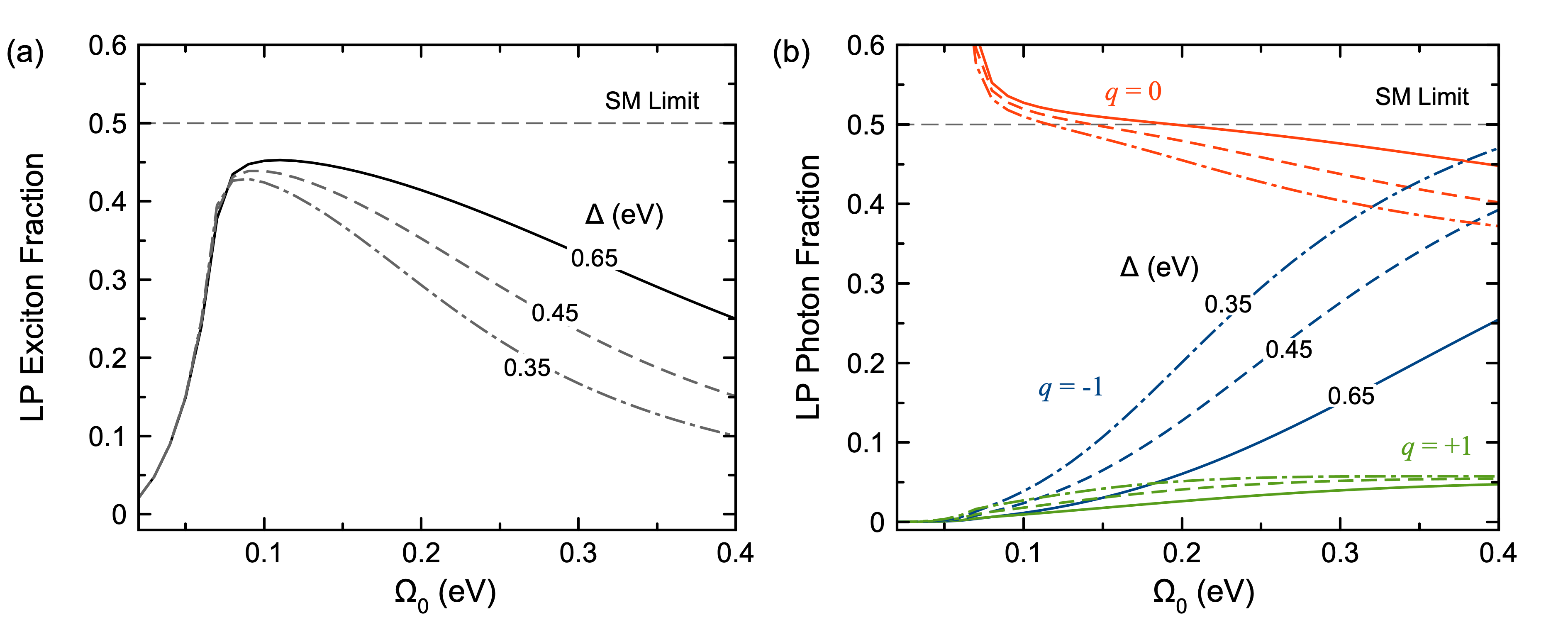
Figure 4: Modified polariton wavefunctions in low finesse cavities: (a) Exciton fraction of the LP state as a function of the bare Rabi coupling for a three-mode cavity with realistic parameters ($\Delta\approx 0.65$ eV Thomas_AdvMat_2024_36_2309393 ). The single-mode (SM) limit for $q=0$ resonant with the dipoles is marked. Results for other values of $\Delta$ are also shown, keeping other parameters the same. (b) Photon fraction per $q$-mode of the LP state as a function bare Rabi coupling for different values of $\Delta$, using the same parameters in (a).

Similar to the adiabatic corrections in Eq. (16), the changes of the polariton decay rates $\Gamma_{\pm}$ predicted for low-finesse cavities also scale linearly with the difference in bandwidth $\Delta\kappa_{q}$ of nearby modes relative to the near-resonant $q=0$ mode. However, whilst adiabatic bandwidth corrections vanish for systems with mode-independent Rabi couplings, Eq. (21) suggests that the mode-order dependence of the bare bandwidths is more important than variations in the field profile (Rabi coupling) of different cavity modes to establish the bandwidths of the LP and UP resonances.

Figure 3a shows the Rabi splitting $\Omega_{R}$ (in eV) predicted by Eq. (20) as function of the bare Rabi coupling $\Omega_{0}$ with the central mode ($\Omega_{q}=\Omega$) and the FSR $\Delta$, for a system with decreasing mode bandwidth with increasing mode order ($\zeta=-0.1$ eV). Even for relatively large values of $\Delta\sim 1{\rm eV}$, the direct interaction of dipoles with $q=\pm 1$ modes significantly reduces the multi-mode Rabi splitting from the usual single-mode value $\Omega_{R}^{\rm SM}=2\Omega_{0}$. In practical terms, the requirements for establishing a light-matter interaction strength that gives a desired polariton splitting become more demanding as the finesse decreases. Figure 3b shows the complementary effect on the LP and UP bandwidths $\Gamma_{\pm}$ given by Eq. (21), as functions of $\Delta$. The bare mode bandwidth is $\kappa=0.15$ eV and a small linear decrease of the bandwidth with mode order is assumed ($\zeta=-50$ meV). The polariton level (UP) closer in frequency to the narrower mode ($q=+1$), becomes narrower as $\Delta$ decreases, and the level (LP) closer to the broader mode ($q=-1$) broadens. Even for relatively large mode separations ($\Delta=1.2$eV, $\mathcal{F}\approx 8$), the LP and UP bandwidths are asymmetric and can differ significantly from the single-mode prediction $\Gamma_{\pm}^{\rm SM}=(\kappa+\gamma)/2$. The deviation from $\Gamma_{\pm}^{\rm SM}$ grows with increasing coupling strength $\Omega_{0}$.

In addition to the changes in Rabi splitting and polariton bandwidths introdcude by the direct interaction of dipoles with neighbouring modes, the microscopic composition of the LP and UP polariton wavefunctions can be very different in low-finesse cavities relative to a single-mode picture. Understanding this can improve the ability to control the emission properties of organic microcavities Herrera2017-PRA ; Herrera_PRL_2017_118_223601 .

In an ideal single-mode cavity under strong coupling conditions $\Omega_{R}>(\kappa_{0}+\gamma)/2$, the LP and UP states can be accurately described Eq. (11) with $|\beta|=|\alpha|=1/2$, i.e., equal exciton and photon content. For the three-mode problem centered around $q=0$, molecular dipoles can also admix with the lower- and higher-order modes $q=\pm 1$. Therefore, a more realistic description of LP and UP states would be

$$\ket{\psi} = \beta\ket{X}\ket{0_{0}}$$

$$+\ket{G}\otimes\left(\alpha_{-1}\ket{1_{-1}}+\alpha_{0}\ket{1_{0}}+\alpha_{+1}\ket{1_{+1}}\right)$$

where $\ket{n_{q}}$ denotes a Fock state of the $q$-th cavity mode and $\ket{G}=\ket{g_{1}g_{2},\ldots,g_{N}}$. $|\beta|^{2}$ is the exciton fraction and $|\alpha_{q}|^{2}$ the fraction of the $q$-th cavity mode in the polariton state. Equation (V) highlights that dipoles exchange energy and coherence with a single-photon wavepacket, not an individual Fock state. Since $\ket{\psi}$ is normalized, the photon fraction associated with the near-resonant mode $|\alpha_{0}|^{2}=1-|\beta|^{2}-|\alpha_{-1}|^{2}-|\alpha_{+1}|^{2}$ is always smaller than the single-mode limit ($\Delta\rightarrow\infty,\alpha_{\pm 1}\rightarrow 0$). The continuous-variable version of the single-photon wavepacket in Eq. (V) arises naturally when describing dipole emission in macroscopic QED Feist2021 ; Medina2021 .

Figure 4a shows the material (exciton) content of the LP state as a function of the bare coupling $\Omega_{0}$, obtained from the eigenvectors of the three-mode matrix $M$ in Eq. (17), parametrised with realistic frequencies and bandwidths from Ref. Thomas_AdvMat_2024_36_2309393 ($\omega_{e}=2.15$ eV, $\gamma=0.37$ eV, $\omega_{-1}=1.45$ eV, $\omega_{0}=2.14$ eV, $\omega_{+1}=2.76$ eV, $\kappa_{-1}=38$ meV, $\kappa_{0}=90$ meV, $\kappa_{+1}=90$ meV). $\Omega_{0}=\Omega_{\pm 1}$ is a free parameter. The $q=-1$ mode is significantly narrower than $q=0$, but no significant variation is seen for $q=1$. The standard single-mode picture of strong coupling suggests that for Rabi splittings $\Omega_{R}>(\kappa_{0}+\gamma)/2\approx 0.24$ eV ($\Omega_{0}>0.12$ eV) the exciton fraction should be $|\beta|^{2}\approx 0.5$. In contrast, the exciton fraction of the LP state in Fig. 4a decreases with increasing Rabi coupling. We also show results for a hypothetical scenario where the lower and higher-order mode frequencies are varied as $\omega_{\pm 1}^{\prime}=\omega_{\pm 1}\mp\varepsilon$ (reducing $\Delta$), with all other parameters kept constant . We find that even for moderate values of cavity finesse $\Delta/\kappa\sim 4-5$, the exciton fraction of the LP can be lower than 30% even when the Rabi coupling $\Omega_{0}$ exceeds the bare bandwidths $\kappa_{0}$ and $\gamma$ ($\Omega_{0}>0.3$ eV, $\Omega_{R}>0.5$ eV).

Figure 4b shows a complementary view of the photon content per mode of the LP state, for the same system parameters in Fig. 4a. As the bare Rabi coupling increases, the contribution of the $q=0$ mode decreases below the single-mode limit and the $q=-1$ contribution increases significantly. The changes in the $q=0$ and $q=-1$ components with $\Omega_{0}$ are stronger with decreasing inter-mode separation $\Delta$. The higher-order $q=+1$ state component is less sensitive to $\Omega_{0}$ and $\Delta$, because it is further detuned from the LP.

VI Conclusion and Outlook

It has been understood for many years that taking account of some of the real world complexities, especially disorder, is important in building up a full conceptual model of molecular strong coupling. In this contribution we have shown that it is also important to take into account off-resonance photonic modes supported by a cavity if one is to properly understand molecular strong coupling. In particular we have shown that in low-finesse situations the extent of light-matter mixing (hybridisation) is altered. When adjacent photonic modes are spectrally overlapped then the molecular content (here we considered excitons) is spread over several photonic modes, resulting in a lower matter content in any given polariton mode. This conclusion is supported by a similar finding in the context of circuit QED Sundaresan_PRX_2015_5_021035 . We have also shown that the extent of the Rabi-splitting can be curtailed by the effect of extra photonic modes.

Looking ahead it will be important to explore these issues further, especially in conjunction with experiment. We have already made a start in this direction menghrajani2024 , where we monitored luminescence from a range of planar samples, since luminescence probes the extent of light-matter mixing more directly that, for example, reflectivity. It would be useful to build on this start with a more systematic study. For example, one could envisage a series of experiments on Fabry Perot planar cavities that employ metal mirrors, where the metal-mirror thickness is altered to control the cavity mode-width, and hence the finesse.

Regarding development of the model that we have outlined here, future extensions should include frequency disorder of dipole transitions, which in most cases is the dominant contribution to material absorption lineshape Spano2010 . Disorder leads to the formation of semi-localized states in the spectral region where the uncoupled dipoles also absorb Dubail2022 ; Wellnitz2022 , adding complexity to the analysis of spectroscopic signals not present in the homogeneous dipole (Dicke) models we discussed here. We anticipate that disorder will introduce quantitative changes to the dependence with finesse of the polariton splitting and polariton bandwidths relative to the homogeneous model predictions here, but we the qualitative physics should remain. We already find evidence of the reduction of the exciton content of exciton-polariton states due to multimode light-matter interaction in a realistically disordered system menghrajani2024 . A more general theoretical framework should be able to treat the simultaneous coupling of molecular dipoles to multiple discrete transverse modes and continuous in-plane momenta in a microcavity. Such a theory would be complex, but may enable studies of controlled excitation transport along a polariton branch by possibly driving off-resonant coupled photonic branches with external fields.

VII Acknowledgements

WAB acknowledge the support of European Research Council through the photmat project (ERC-2016-AdG-742222 :www.photmat.eu). FH acknowledges the support of the Royal Society through the award of a Royal Society Wolfson Visiting Fellowship, and ANID through grants Fondecyt Regular 1221420, Millennium Science Initiative Program ICN17_012, and the Air Force Office of Scientific Research under award number FA9550-22-1-0245.

Appendix A Adiabatic elimination of far-detuned cavity modes

In this section we derive Eq. (12) in the main text.

The non-degenerate ground state has no excitations in the electronic and cavity modes and is given by $\ket{\psi^{(0)}}=\ket{g_{1}g_{2},\ldots,g_{N}}\ket{0_{-K},\ldots,0_{-1},0_{0},0_{+1},\ldots,0_{K}}$. $M=2K+1$ discrete transverse modes are considered. The single-excitation electron-photon wavefunction can be written as

$$\ket{\psi^{(1)}}=\sum_{i}c_{i}^{(0)}\ket{e_{i}}\ket{\{0_{q}\}}+\sum_{q}\,c_{q}^{(1)}\ket{g_{1}g_{2},\ldots,g_{N}}\ket{1_{q}},$$ (23)

where $\ket{\{0_{q}\}}$ is the multi-mode cavity vacuum, $\ket{e_{i}}$ describes a single excitation in the $i$-th molecule with all the other dipoles in the ground state, and $\ket{1_{q}}$ describes a single photon in the $q$-th mode, with all the other modes in the vacuum state. There are no other restrictions on the material and photonic coefficients $c_{i}^{(0)}$ and $c_{q}^{(1)}$ except for normalization $\sum_{i}|c_{i}^{(0)}|^{2}+\sum_{q}|c_{q}^{(1)}|^{2}=1$.

We derive evolution equations for the material and photonic wavepacket amplitudes $c_{i}^{(0)}$ and $c_{q}^{(1)}$ from the single-excitation ansatz (23), directly from the non-Hermitian Schrödinger equation $(d/dt)\ket{\psi^{1}}=-i\hat{\mathcal{H}}_{\rm eff}\ket{\psi^{(1)}}$, with $\hat{\mathcal{H}}_{\rm eff}$ given by Eq. (5). Rewriting the state amplitudes as $c_{j}^{(0)}=\tilde{c}_{j}^{(0)}\,{\rm exp}[-i\tilde{\omega}_{0}t]$ and $c_{q}^{(1)}=\tilde{c}_{q}^{(1)}\,{\rm exp}[-i\tilde{\omega}_{0}t]$, where $\tilde{\omega}_{0}=\omega_{0}-i\kappa_{0}/2$ is the complex frequency of the free $q=0$ mode. In this new $q=0$ frame, we obtain the following system of $(M+N)$ coupled equations for the amplitudes

$$\frac{d}{dt}\tilde{c}_{j}^{(0)} = (i\delta_{j}+\Delta\gamma_{j}/2)\tilde{c}_{j}^{(0)}-i\sum_{q}g_{jq}\tilde{c}_{q}^{(1)}$$ (24)

$$\frac{d}{dt}\tilde{c}_{q}^{(1)} = -(i\Delta_{q}+\Delta\kappa_{q}/2)\tilde{c}_{q}^{(1)}-i\sum_{j}g_{jq}^{*}\tilde{c}_{j}^{(0)},$$ (25)

where $\delta_{j}=\omega_{0}-\omega_{j}$ is the detuning of the reference ($q=0$) mode relative to the $i$-th dipole frequency, $\omega_{q}=\omega_{0}+\Delta_{q}$ is the frequency of the $q$-th higher ($\Delta_{q}>0$) or lower order mode ($\Delta_{q}<0$) relative to $q=0$. $\Delta\gamma_{j}=\kappa_{0}-\gamma_{j}$ is the decay mismatch between dipoles and the reference mode, and $\Delta\kappa_{q}=\kappa_{q}-\kappa_{0}$ is decay mismatch relative to $q=0$.

We derive a reduced set of coupled equations of motion for the $N$ excited state amplitudes $\tilde{c}_{j}^{(0)}$ and the single-photon amplitude of the reference mode $\tilde{c}_{0}{(1)}$, under the assumption that modes that only the reference mode $q=0$ interacts resonantly with the dipolar ensemble, but higher and lower order modes ($q\neq 0$) are sufficiently detuned from the dipole frequencies $\omega_{j}$ to prevent significantly exchange of energy and coherence between light and matter. In this case, the off-resonant modes simply follow adiabatically the dipole polarization to lowest order in $g_{jq}$. The stationary off-resonant mode amplitude is obtained from Eq. (25) to give

$$\tilde{c}_{q\neq 0}^{(1)}=-i\sum_{i=1}^{N}\frac{g_{iq}^{*}\,\tilde{c}_{i}^{(0)}}{i\Delta_{q}+\Delta\kappa_{q}/2}.$$ (26)

Separating Eqs. (24) and (25) into resonant ($q=0$) and non-resonant mode contributions, and inserting the adiabatic solution in Eq. (26) for the lower and higher order modes, we obtain a reduced set of ($1+N$) equations of motion of the form

$$\frac{d}{dt}\tilde{c}_{j}^{(0)} = i(\delta_{j}-\Gamma_{j}^{{}^{\prime\prime}})\tilde{c}_{j}^{(0)}+(\Delta\gamma_{j}/2-\Gamma_{j}^{\prime})\tilde{c}_{j}^{(0)}-ig_{j0}\tilde{c}_{0}^{(1)}-\sum_{i\neq j}(J_{ij}^{\prime}+iJ_{ij}^{{}^{\prime\prime}})\tilde{c}_{i}^{(0)}$$ (27)

$$\frac{d}{dt}\tilde{c}_{0}^{(1)} = -i\sum_{i}g_{i0}^{*}\,\tilde{c}_{i}^{(0)}$$ (28)

where we introduced the effective one-body and two-body decay rates,

$$\Gamma_{j}^{\prime} = -\sum_{q\neq 0}|g_{jq}|^{2}\frac{\Delta\kappa_{q}/2}{\Delta_{q}^{2}+(\Delta\kappa_{q}/2)^{2}},$$ (29)

$$J_{ij}^{\prime} = -\sum_{q\neq 0}g_{iq}^{*}g_{jq}\frac{\Delta\kappa_{q}/2}{\Delta_{q}^{2}+(\Delta\kappa_{q}/2)^{2}},$$ (30)

and effective frequency shifts given by

$$\Gamma_{j}^{{}^{\prime\prime}} = -\sum_{q\neq 0}|g_{jq}|^{2}\frac{\Delta_{q}}{\Delta_{q}^{2}+(\Delta\kappa_{q}/2)^{2}},$$ (31)

$$J_{ij}^{\prime\prime} = -\sum_{q\neq 0}g_{iq}^{*}g_{jq}\frac{\Delta_{q}/2}{\Delta_{q}^{2}+(\Delta\kappa_{q}/2)^{2}}.$$ (32)

In these expressions, the sum-over-modes exclude the reference $q=0$ cavity resonance. The reduced equations of motion (27) and (28) can accurately describe strong coupling between the $N$ oscillators and the near-resonant $q=0$ mode, and improves over previous treatments in the literature by including the effect of far-detuned higher and lower order modes self-consistently. The quasi-static solution for non-resonant modes in Eq. (26) is accurate for modes that do not significantly admix with dipole transitions, which requires $|\Delta_{q}|>\sqrt{\sum_{j}|g_{jq}|^{2}}$ for each $q\neq 0$.

In the idealized Dicke regime where the $N$ dipoles have equal transition frequencies ($\omega_{i}=\omega_{e}$), Rabi couplings ($g_{iq}=g_{q}$) and relaxation rates ($\gamma_{i}=\gamma$), the reduced dynamical equations (27) and (28) further simplify by writing $\tilde{c}_{i}=\beta/\sqrt{N}$ and $\tilde{c}_{0}=\alpha_{0}$. The evolution equation for the collective dipole coherence $\tilde{X}=\sum_{i}\tilde{c}_{i}^{(0)}=\sqrt{N}\beta$, can be obtained by summing Eq. (27) over all dipoles to obtain two coupled equations for $\alpha_{0}$ and $\beta$ that can be written in matrix form as

$$\left(\begin{array}[]{c}\dot{\alpha}_{0}\\ \dot{\beta}\end{array}\right)=\left(\begin{array}[]{cc}0&-i\sqrt{N}g_{0}\\ -i\sqrt{N}g_{0}&i\delta_{N}-\Delta\Gamma_{N}\end{array}\right)\left(\begin{array}[]{c}\alpha_{0}\\ \beta\end{array}\right),$$ (33)

with

$$\delta_{N} = \delta_{0}-\Gamma{{}^{\prime\prime}}-NJ{{}^{\prime\prime}}$$ (34)

$$\Delta\Gamma_{N} = -\Delta\gamma/2+\Gamma^{\prime}+NJ{{}^{\prime}}.$$ (35)

This is Eq. (12) in the main text. $\delta_{0}=\omega_{0}-\omega_{e}$, $\Delta\gamma=\kappa_{0}-\gamma$, and $g_{0}$ refer to properties of the near-resonant $q=0$ mode.

Appendix B Approximate Rabi splitting and polariton bandwidths in low-finesse three-mode cavities

In this section we derive Eqs. (20) and (21) in the main text.

We consider a three-mode cavity model with a central $q=0$ mode at $\omega_{0}$ tuned near resonance with a homogeneous ensemble of $N$ dipole transitions at $\omega_{e}$. The dipoles also couple to the lower-order mode $q=-1$ and a higher-order mode $q=+1$, with frequencies $\omega_{\pm 1}=\omega_{0}\pm\Delta_{\pm 1}$, respectively. The evolution equations (24)-(25) reduce in this case to a (3+1) system for the collective coherence $\tilde{X}=\sum_{j}\tilde{c}_{j}^{0}=\sqrt{N}\beta$, ($\delta_{j}=\delta_{0}$, $\Delta\gamma_{j}=\Delta\gamma$, $g_{jq}=g_{q}$) and photon amplitudes $\tilde{c}_{q}^{(1)}\equiv\alpha_{q}$, with $q=\{-1,0,1\}$. The resulting system of equations can be written in matrix form as $\dot{\mathbf{x}}=-i\mathbf{M}\,\mathbf{x}$, with $\mathbf{x}=[\alpha_{+1},\alpha_{0},\alpha_{-1},\beta]^{\rm T}$ and $\mathbf{M}$ written in arrowhead form as ,

$$\mathbf{M}=\left(\begin{array}[]{cccc}\Delta_{-1}-i\Delta\kappa_{-1}/2&0&0&\Omega_{-1}\\ 0&0&0&\Omega_{0}\\ 0&0&\Delta_{+1}-i\Delta\kappa_{+1}/2&\Omega_{+1}\\ \Omega_{-1}&\Omega_{0}&\Omega_{+1}&-\delta+i\Delta\gamma/2\\ \end{array}\right)\equiv\left(\begin{array}[]{cccc}d_{-1}&0&0&e_{-1}\\ 0&0&0&e_{0}\\ 0&0&d_{+1}&e_{+1}\\ e_{-1}&e_{0}&e_{+1}&p\\ \end{array}\right),$$ (36)

where $\Omega_{q}=\sqrt{N}g_{q}$ (with $g_{q}=g_{q}^{*}$), $\delta=\omega_{0}-\omega_{e}$, $\Delta\gamma=\kappa_{0}-\gamma$, $\Delta\kappa_{q}=\kappa_{q}-\kappa_{0}$,and $\Delta_{q}=\omega_{q}-\omega_{0}$. We introduced a simplified notation in the second equality. The complex eigenvalues $\lambda=E+i\Gamma/2$ of $\mathbf{M}$ are roots of the characteristic polynomial OLeary:1990

$$\Phi(\lambda)\equiv p-\lambda+\frac{e_{0}^{2}}{\lambda}-\frac{e_{-1}^{2}}{d_{-1}-\lambda}-\frac{e_{+1}^{2}}{d_{+1}-\lambda}.$$ (37)

We are interested in corrections to the polariton splitting $\Omega_{R}\equiv{\rm Re}[\lambda_{\rm UP}]-{\rm Re}[\lambda_{\rm LP}]$ and bandwidths $\Gamma_{\rm LP}=2{\rm Im}[\lambda_{\rm LP}]$, $\Gamma_{\rm UP}=2{\rm Im}[\lambda_{\rm UP}]$, from their values in a single-mode scenario where $q=0$ is resonant with the dipoles ($\delta\approx 0$). Corrections are due to the presence of the adjacent $q=\pm 1$ modes. We thus solve for $x$ in $\Phi(\lambda_{\pm}+x)=0$, where $\lambda_{\pm}$ denotes the pair of coupled single-mode solutions to Eq. (37) obtained for $\Omega_{\pm 1}=0$, giving $\lambda_{\pm}(p-\lambda_{\pm})+e_{0}^{2}=0$. For $\Delta\gamma=\delta=0$ ($p=0$), the single-mode LP and UP solutions are $\lambda_{\pm}=\pm\Omega_{0}$, giving the bare splitting $\Omega_{R}=2\Omega_{0}$ and bandwidths $\Gamma_{\rm LP}=\Gamma_{\rm UP}=\kappa$.

Linearizing the polynomial $\Phi(\lambda_{\pm}+x)=0$ around $x=0$ gives the general solution,

$$x_{\pm}=\frac{-\lambda_{\pm}[e_{-1}^{2}d_{+1}+e_{+1}^{2}d_{-1}-(e_{-1}^{2}+e_{+1}^{2})\lambda_{\pm}]}{P(\lambda_{\pm})},$$ (38)

with

$$P(\lambda_{\pm}) = d_{+1}(e_{0}^{2}+e_{-1}^{2})+d_{-1}(e_{0}^{2}+e_{+1}^{2})-d_{-1}d_{+1}p-2(e_{0}^{2}+e_{-1}^{2}+e_{+1}^{2}-d_{+1}p-d_{-1}p-d_{-1}d_{+1})\lambda_{\pm}$$ (39)

$$-3(d_{-1}+d_{+1}+p)\lambda_{\pm}^{2}+4\lambda_{\pm}^{3}.$$

The solution $\lambda_{\rm LP}=\lambda_{-}+x_{-}$ gives the LP frequency and decay rate and $\lambda_{\rm UP}=\lambda_{+}+x_{+}$ gives the UP properties. The denominator $P(\lambda_{\pm})$ can be reduced by setting $p=0$, which holds for a resonant single-mode scenario ($\delta_{0}=0$) without decay mismatch ($\Delta\gamma=0$), giving

$$x_{\pm}=-\lambda_{\pm}\times\frac{d_{+1}e_{-1}^{2}+d_{-1}e_{+1}^{2}-\lambda_{\pm}(e_{-1}^{2}+e_{+1}^{2})}{d_{+1}(e_{0}^{2}+e_{-1}^{2})+d_{-1}(e_{0}^{2}+e_{+1}^{2})-2(e_{0}^{2}+e_{+1}^{2}+e_{-1}^{2}-d_{-1}d_{+1})\lambda_{\pm}-3(d_{-1}+d_{+1})\lambda_{\pm}^{2}+4\lambda_{\pm}^{3}}.\\$$

For the special case where there are no mode-order variations of the Rabi coupling and cavity mode bandwidth, i.e., $\Omega_{q}=\Omega$ and $\kappa_{q}=\kappa$ for all $q$, and assuming modes that are equally spaced ($\Delta_{\pm}=\pm\Delta$), we have $d_{+1}e_{-1}^{2}+d_{-1}e_{+1}^{2}=+\Delta\Omega^{2}-\Delta\Omega^{2}=0$ in Eq. (B) and corrections to the LP and UP eigenvalues become purely real

$$x_{\pm}=-\lambda_{\pm}\,\frac{\Omega^{2}}{3\Omega^{2}+\Delta^{2}-2\lambda_{\pm}^{2}}=\mp\Omega\left(\frac{\Omega^{2}}{\Omega^{2}+\Delta^{2}}\right),$$ (40)

with $\Delta>\Omega$ and $\lambda_{\pm}=\pm\Omega$. Therefore, without mode-order variations of the cavity parameters, level pushing from the higher-order and lower-order modes gives the reduced Rabi splitting

$$\Omega_{R}=2\Omega+x_{+}-x_{-}=2\Omega\left(\frac{\Delta^{2}}{\Delta^{2}+\Omega^{2}}\right),$$ (41)

but there no changes to the polariton bandwidths relative to the single-mode scenario.

The simplest ideal scenario with corrections to the LP and UP bandwidths is one where the Rabi couplings do not depend on mode order ($\Omega_{p}=\Omega$), but cavity modes can differ in bandwidth ($\Delta\kappa_{q}\neq 0$). From Eq. (B), neglecting quadratic terms in $\Delta\kappa_{\pm 1}$ relative to $\Delta^{2}+\Omega^{2}$, we obtain in this case,

$${\rm Re}[x_{\pm}]\approx\mp\Omega\,\frac{\Omega^{2}(\Omega^{2}+\Delta^{2})^{2}}{(\Omega^{2}+\Delta^{2})^{2}+(\Delta(\Delta\kappa_{-1}-\Delta\kappa_{+1})\mp\Omega(\Delta\kappa_{-1}+\Delta\kappa_{+1})/2)^{2}},$$ (42)

and,

$$2{\rm Im}[x_{\pm}]=\mp\Omega\,\frac{\Omega(\Delta\kappa_{-1}+\Delta\kappa_{+1})(\Omega^{2}+\Delta^{2})/2\pm\Omega^{2}[\Delta(\Delta\kappa_{-1}-\Delta\kappa_{+1})\mp\Omega(\Delta\kappa_{-1}+\Delta\kappa_{+1})/2]}{(\Omega^{2}+\Delta^{2})^{2}+(\Delta(\Delta\kappa_{-1}-\Delta\kappa_{+1})\mp\Omega(\Delta\kappa_{-1}+\Delta\kappa_{+1})/2)^{2}}.$$ (43)

From these expressions we may obtain the lower and upper polariton energies $E_{\pm}=\pm\Omega+{\rm Re}[x_{\pm}]$ and decay rates $\Gamma_{\pm}=\kappa+2{\rm Im}[x_{\pm}]$. For linear changes in mode bandwidth of the form $\Delta\kappa_{q}=q\zeta$, with $\zeta$ positive or negative, the LP and UP energies can then be written as,

$$E_{\pm}=\pm\Omega\left[1-\frac{\Omega^{2}(\Omega^{2}+\Delta^{2})}{(\Omega^{2}+\Delta^{2})^{2}+\Delta^{2}\zeta^{2}}\right],$$ (44)

from where Eq. (20) in the main text is obtained. From Eq. (43), the polariton bandwidths for linear bandwidth changes with mode order are thus

$$\Gamma_{\pm}=\kappa\pm 2\Omega\frac{\Omega^{2}\Delta\zeta}{(\Omega^{2}+\Delta^{2})^{2}+\Delta^{2}\zeta^{2}},$$ (45)

which is Eq. (21) in the main text.

References

- [1] D. G. Lidzey, D. D. C. Bradley, T. Virgil, A. Armitage, M. S. Skolnick, and S. Walker. Room temperature polariton emission from strongly coupled organic semiconductor microcavities. Physical Review Letters, 82(16):3316–3319, 1999.
- [2] Felipe Herrera and Jeffrey Owrutsky. Molecular polaritons for controlling chemistry with quantum optics. The Journal of Chemical Physics, 152:100902, 2020.
- [3] Mónica Sánchez-Barquilla, Antonio I. Fernández-Domínguez, Johannes Feist, and Francisco J. García-Vidal. A theoretical perspective on molecular polaritonics. ACS Photonics, 9(6):1830–1841, 2022.
- [4] Arkajit Mandal, Michael A.D. Taylor, Braden M. Weight, Eric R. Koessler, Xinyang Li, and Pengfei Huo. Theoretical advances in polariton chemistry and molecular cavity quantum electrodynamics. Chemical Reviews, 123(16):9786–9879, 2023. PMID: 37552606.
- [5] Rahul Bhuyan, Maksim Lednev, Johannes Feist, and Karl Börjesson. The effect of the relative size of the exciton reservoir on polariton photophysics. Advanced Optical Materials, 12(2):2301383, 2024.
- [6] Thomas Khazanov, Suman Gunasekaran, Aleesha George, Rana Lomlu, Soham Mukherjee, and Andrew J. Musser. Embrace the darkness: An experimental perspective on organic exciton–polaritons. Chemical Physics Reviews, 4(4):041305, 11 2023.
- [7] F. C. Spano. Optical microcavities enhance the exciton coherence length and eliminate vibronic coupling in J-aggregates. The Journal of Chemical Physics, 142(18):184707, 05 2015.
- [8] Ćwik, Justyna A., Reja, Sahinur, Littlewood, Peter B., and Keeling, Jonathan. Polariton condensation with saturable molecules dressed by vibrational modes. EPL, 105(4):47009, 2014.
- [9] Felipe Herrera and Frank C. Spano. Cavity-controlled chemistry in molecular ensembles. Phys. Rev. Lett., 116:238301, 2016.
- [10] Felipe Herrera and Frank C. Spano. Dark vibronic polaritons and the spectroscopy of organic microcavities. Phys. Rev. Lett., 118:223601, May 2017.
- [11] Felipe Herrera and Frank C. Spano. Absorption and photoluminescence in organic cavity QED. Phys. Rev. A, 95:053867, 2017.
- [12] Javier del Pino, Florian A. Y. N. Schröder, Alex W. Chin, Johannes Feist, and Francisco J. Garcia-Vidal. Tensor network simulation of non-markovian dynamics in organic polaritons. Phys. Rev. Lett., 121:227401, Nov 2018.
- [13] Michael Ruggenthaler, Johannes Flick, Camilla Pellegrini, Heiko Appel, Ilya V. Tokatly, and Angel Rubio. Quantum-electrodynamical density-functional theory: Bridging quantum optics and electronic-structure theory. Phys. Rev. A, 90:012508, Jul 2014.
- [14] Johannes Flick, Michael Ruggenthaler, Heiko Appel, and Angel Rubio. Atoms and molecules in cavities, from weak to strong coupling in quantum-electrodynamics (qed) chemistry. Proceedings of the National Academy of Sciences, 114(12):3026–3034, 2017.
- [15] Hoi Ling Luk, Johannes Feist, J. Jussi Toppari, and Gerrit Groenhof. Multiscale molecular dynamics simulations of polaritonic chemistry. Journal of Chemical Theory and Computation, 13(9):4324–4335, Aug 2017.
- [16] V. M. Agranovich, M. Litinskaia, and D. G. Lidzey. Cavity polaritons in microcavities containing disordered organic semiconductors. Physical Review B, 67(8):085311, Feb 2003.
- [17] Raphael F. Ribeiro. Multimode polariton effects on molecular energy transport and spectral fluctuations. Communications Chemistry, 5(1):48, 2022.
- [18] Jonathan Keeling and Stéphane Kéna-Cohen. Bose–einstein condensation of exciton-polaritons in organic microcavities. Annual Review of Physical Chemistry, 71(Volume 71, 2020):435–459, 2020.
- [19] Kristin B. Arnardottir, Antti J. Moilanen, Artem Strashko, Päivi Törmä, and Jonathan Keeling. Multimode organic polariton lasing. Phys. Rev. Lett., 125:233603, Dec 2020.
- [20] Jino George, Thibault Chervy, Atef Shalabney, Eloïse Devaux, Hidefumi Hiura, Cyriaque Genet, and Thomas W. Ebbesen. Multiple rabi splittings under ultrastrong vibrational coupling. Physical Review Letters, 117(15):153601, Oct 2016.
- [21] Philip A. Thomas and William L. Barnes. Strong coupling-induced frequency shifts of highly detuned photonic modes in multimode cavities. The Journal of Chemical Physics, 160(20):204303, 05 2024.
- [22] Neereja M. Sundaresan, Yanbing Liu, Darius Sadri, Laszlo J. Szocs, Devin L. Underwood, Moein Malekakhlagh, Hakan E. Tureci, and Andrew A. Houck. Beyond strong coupling in a multimode cavity. Physical Review X, 5(2):021035, Jun 2015.
- [23] Kishan S. Menghrajani, Adarsh B. Vasista, Wai Jue Tan, Philip A. Thomas, Felipe Herrera, and William L. Barnes. Molecular strong coupling and cavity finesse, 2024.
- [24] David M. Coles and David G. Lidzey. A ladder of polariton branches formed by coupling an organic semiconductor exciton to a series of closely spaced cavity-photon modes. Applied Physics Letters, 104(19):191108, 05 2014.
- [25] Kyriacos Georgiou, Kirsty E. McGhee, Rahul Jayaprakash, and David G. Lidzey. Observation of photon-mode decoupling in a strongly coupled multimode microcavity. The Journal of Chemical Physics, 154(12):124309, 03 2021.
- [26] M. Godsi, A. Golombek, M. Balasubrahmaniyam, and T. Schwartz. Exploring the nature of high-order cavity polaritons under the coupling–decoupling transition. The Journal of Chemical Physics, 159(13):134307, 10 2023.
- [27] A. Shalabney, J. George, J. Hutchison, G. Pupillo, C. Genet, and T. W. Ebbesen. Coherent coupling of molecular resonators with a microcavity mode. Nature Communications, 6(1):1–6, Jan 2015.
- [28] B. S. Simpkins, Kenan P. Fears, Walter J. Dressick, Bryan T. Spann, Adam D. Dunkelberger, and Jeffrey C. Owrutsky. Spanning strong to weak normal mode coupling between vibrational and fabry–pérot cavity modes through tuning of vibrational absorption strength. ACS Photonics, 2(10):1460–1467, Oct 2015.
- [29] Manuel Hertzog and Karl Börjesson. The effect of coupling mode in the vibrational strong coupling regime. ChemPhotoChem, 4(8):612–617, 2020.
- [30] Mukundakumar Balasubrahmaniyam, Arie Simkhovich, Adina Golombek, Gal Sandik, Guy Ankonina, and Tal Schwartz. From enhanced diffusion to ultrafast ballistic motion of hybrid light–matter excitations. Nature Materials, 22(3):338–344, 2023.
- [31] Nicholas J Hestand and Frank C Spano. Expanded theory of h-and j-molecular aggregates: the effects of vibronic coupling and intermolecular charge transfer. Chemical reviews, 118(15):7069–7163, 2018.
- [32] P. A. Hobson, W. L. Barnes, D. G. Lidzey, G. A. Gehring, D. M. Whittaker, M. S. Skolnick, and S. Walker. Strong exciton–photon coupling in a low-Q all-metal mirror microcavity. Applied Physics Letters, 81(19):3519–3521, 2002.
- [33] Daqing Wang, Hrishikesh Kelkar, Diego Martin-Cano, Dominik Rattenbacher, Alexey Shkarin, Tobias Utikal, Stephan Götzinger, and Vahid Sandoghdar. Turning a molecule into a coherent two-level quantum system. Nature Physics, 15:483–489, 2019.
- [34] M. S. Skolnick, T. A. Fisher, and D. M. Whittaker. Strong coupling phenomena in quantum microcavity structures. Semiconductor Science and Technology, 13(7):645, 1998.
- [35] Daqing Wang, Hrishikesh Kelkar, Diego Martin-Cano, Dominik Rattenbacher, Alexey Shkarin, Tobias Utikal, Stephan Götzinger, and Vahid Sandoghdar. Turning a molecule into a coherent two-level quantum system. Nature Physics, 15(5):483–489, 2019.
- [36] D. G. Lidzey, D. D. C. Bradley, M. S. Skolnick, T. Virgili, S. Walker, and D. M. Whittaker. Strong exciton-photon coupling in an organic semiconductor microcavity. Nature, 395(6697):53–55, 09 1998.
- [37] W. L. Barnes. Fluorescence near interfaces: The role of photonic mode density. Journal of Modern Optics, 45:661–699, 1998.
- [38] S. Kéna-Cohen, M. Davanço, and S. R. Forrest. Strong exciton-photon coupling in an organic single crystal microcavity. Phys. Rev. Lett., 101:116401, Sep 2008.
- [39] Felipe Herrera and Frank C. Spano. Theory of nanoscale organic cavities: The essential role of vibration-photon dressed states. ACS Photonics, 5:65–79, 2018.
- [40] Frank C. Spano. Exciton–phonon polaritons in organic microcavities: Testing a simple ansatz for treating a large number of chromophores. The Journal of Chemical Physics, 152(20):204113, 05 2020.
- [41] David Hagenmüller, Johannes Schachenmayer, Stefan Schütz, Claudiu Genes, and Guido Pupillo. Cavity-enhanced transport of charge. Phys. Rev. Lett., 119:223601, Nov 2017.
- [42] Georg Engelhardt and Jianshu Cao. Polariton localization and dispersion properties of disordered quantum emitters in multimode microcavities. Phys. Rev. Lett., 130:213602, May 2023.
- [43] Nahum C. Chávez, Francesco Mattiotti, J. A. Méndez-Bermúdez, Fausto Borgonovi, and G. Luca Celardo. Disorder-enhanced and disorder-independent transport with long-range hopping: Application to molecular chains in optical cavities. Phys. Rev. Lett., 126:153201, Apr 2021.
- [44] Stéphane Kéna-Cohen, Stefan A. Maier, and Donal D. C. Bradley. Ultrastrongly coupled exciton–polaritons in metal-clad organic semiconductor microcavities. Advanced Optical Materials, 1(11):827–833, 2013.
- [45] H P. Breuer and F Petruccione. The theory of open quantum systems. Oxford University Press, 2002.
- [46] Klaus Mølmer, Yvan Castin, and Jean Dalibard. Monte carlo wave-function method in quantum optics. J. Opt. Soc. Am. B, 10(3):524–538, Mar 1993.
- [47] J. M. Raimond, M. Brune, and S. Haroche. Manipulating quantum entanglement with atoms and photons in a cavity. Rev. Mod. Phys., 73:565–582, Aug 2001.
- [48] Ian D. Leroux, Monika H. Schleier-Smith, and Vladan Vuletić. Implementation of cavity squeezing of a collective atomic spin. Phys. Rev. Lett., 104:073602, Feb 2010.
- [49] Philip A. Thomas, Wai Jue Tan, Vasyl G. Kravets, Alexander N. Grigorenko, and William L. Barnes. Non-polaritonic effects in cavity-modified photochemistry. Advanced Materials, 36(7):2309393, 2024.
- [50] Johannes Feist, Antonio I. Fernández-Domínguez, and Francisco J. García-Vidal. Macroscopic qed for quantum nanophotonics: emitter-centered modes as a minimal basis for multiemitter problems. Nanophotonics, 10(1):477–489, 2021.
- [51] Ivan Medina, Francisco J. García-Vidal, Antonio I. Fernández-Domínguez, and Johannes Feist. Few-mode field quantization of arbitrary electromagnetic spectral densities. Phys. Rev. Lett., 126:093601, Mar 2021.
- [52] Frank C Spano. The spectral signatures of frenkel polarons in h- and j-aggregates. Acc. Chem. Res., 43(3):429–439, 2010.
- [53] J. Dubail, T. Botzung, J. Schachenmayer, G. Pupillo, and D. Hagenmüller. Large random arrowhead matrices: Multifractality, semilocalization, and protected transport in disordered quantum spins coupled to a cavity. Phys. Rev. A, 105:023714, Feb 2022.
- [54] David Wellnitz, Guido Pupillo, and Johannes Schachenmayer. Disorder enhanced vibrational entanglement and dynamics in polaritonic chemistry. Communications Physics, 5(1):120, 2022.
- [55] D. P O’Leary and G. W Stewart. Computing the eigenvalues and eigenvectors of symmetric arrowhead matrices. Journal of Computational Physics, 90(2):497–505, 1990.
- [56] S. Richter, T. Michalsky, L. Fricke, C. Sturm, H. Frank, M. Grundmann, and R. Schmidt-Grund. Maxwell consideration of polaritonic quasi-particle hamiltonians in multi-level systems. Applied Physics Letters, 107:231104, 2015.