Lyu, Yuan, Zhou, Zhou

Optimality of SAA for Data-Driven Newsvendor Problems

Closing the Gaps: Optimality of Sample Average Approximation for Data-Driven Newsvendor Problems

Jiameng Lyu Department of Mathematical Sciences, Tsinghua University, Beijing 100084, China, lvjm21@mails.tsinghua.edu.cn Shilin Yuan Department of Mathematical Sciences, Tsinghua University, Beijing 100084, China, yuansl21@mails.tsinghua.edu.cn Bingkun Zhou Qiuzhen College, Tsinghua University, Beijing 100084, China, zbk23@mails.tsinghua.edu.cn Yuan Zhou Yau Mathematical Sciences Center & Department of Mathematical Sciences, Tsinghua University, Beijing 100084, China, yuan-zhou@tsinghua.edu.cn

We study the regret performance of Sample Average Approximation (SAA) for data-driven newsvendor problems with general convex inventory costs. In literature, the optimality of SAA has not been fully established under both $\alpha$-global strong convexity and $(\alpha,\beta)$-local strong convexity ($\alpha$-strongly convex within the $\beta$-neighborhood of the optimal quantity) conditions. This paper closes the gaps between regret upper and lower bounds for both conditions. Under the $(\alpha,\beta)$-local strong convexity condition, we prove the optimal regret bound of $\Theta(\log T/\alpha+1/(\alpha\beta))$ for SAA. This upper bound result demonstrates that the regret performance of SAA is only influenced by $\alpha$ and not by $\beta$ in the long run, enhancing our understanding about how local properties affect the long-term regret performance of decision-making strategies. Under the $\alpha$-global strong convexity condition, we demonstrate that the worst-case regret of any data-driven method is lower bounded by $\Omega(\log T/\alpha)$, which is the first lower bound result that matches the existing upper bound with respect to both parameter $\alpha$ and time horizon $T$. Along the way, we propose to analyze the SAA regret via a new gradient approximation technique, as well as a new class of smooth inverted-hat-shaped hard problem instances that might be of independent interest for the lower bounds of broader data-driven problems.

inventory management, newsvendor problem, sample average approximation, online learning, regret analysis

1 Introduction

The newsvendor model, a fundamental problem in operations management, has been extensively applied across various industries such as retailing, manufacturing, and healthcare. In a newsvendor problem, the decision-maker needs to carefully decide the daily order quantity to minimize costs, including underage costs due to unsatisfied demand and overage costs due to excess inventory. With the increasing success of statistical machine learning methods, significant research effort has been devoted to the study of the data-driven newsvendor problem. In this context, the demand distribution is unknown in advance, and the decision-maker collects historical demand data to inform decisions. Among the data-driven methods, Sample Average Approximation (SAA) has gained great popularity in practice due to its simplicity and competitive performance. This popularity has motivated a series of works to advance the theoretical understanding of this simple yet powerful method in data-driven newsvendor problems (Levi et al. 2007, Besbes and Muharremoglu 2013, Levi et al. 2015, Lin et al. 2022).

In a general stochastic optimization problem, SAA decision-makers use historical samples to approximate the objective function under the true distribution, and make decisions by optimizing this empirical objective. The study of SAA has long adopted various structural assumptions of the objective function, e.g., general convexity and $\alpha$-global strong convexity (see Definition 2.2).

In the context of newsvendor problems, demand samples are realized from the demand distribution and the above general assumptions usually hold because of the more specific conditions about the demand distribution. For example, a number of works (Huh and Rusmevichientong 2009, Shi et al. 2016, Zhang et al. 2018, Lyu et al. 2023) have imposed the $\alpha$-global minimal separation condition on the demand distribution to achieve improved logarithmic regret when the overage and underage costs are linear. This condition requires that the PDF of the demand distribution is at least $\alpha$ globally within the optimization domain, which, similarly, together with the linear costs, implies the $\alpha$-global strong convexity of the cost function up to a scaling constant.

A recent work by Lin et al. (2022) introduced the local minimal separation condition, relaxing the global minimal separation condition and aiming to explore the crucial role of local flatness of the demand CDF around the optimal quantity in the regret performance of SAA. Specifically, the $(\alpha,\beta)$-local minimal separation condition specifies that the PDF of the demand distribution is bounded below by a positive constant $\alpha$ within the $\beta$-neighborhood of the optimal quantity, corresponding to the $(\alpha,\beta)$-local strong convexity of the cost function up to a scaling constant.

Lin et al. (2022) established several state-of-the-art theoretical results for data-driven newsvendor problems with linear overage and underage costs under the above two minimal separation conditions. However, despite the significant progress made, the following important problems remain unsolved:

1. The regret analysis in Lin et al. (2022) is tailored for newsvendor problems with linear overage and underage costs. It does not work for the more general convex overage and underage costs. Besides, there is a notable gap between their regret lower bound $\Omega(1/(\alpha\beta))$ for any data-driven policy and their regret upper bound $\mathcal{O}(\log T/(\alpha\beta))$ for SAA, under the $(\alpha,\beta)$-local minimal separation condition.

2. There is no lower bound result that matches the regret upper bound $\mathcal{O}(\log T/\alpha)$ of SAA and SGD simultaneously for the parameter $\alpha$ and the time horizon $T$ under the $\alpha$-global minimal separation condition. Moreover, even without considering $\alpha$, we find that the proof of the widely cited $\Omega(\log T)$ lower bound result in Besbes and Muharremoglu (2013) may be flawed due to a subtle but critical technical oversight.

In this paper, we resolve the above problems via advancing both the upper and lower bounds for SAA (see Table 1 for the summary of our results and comparisons). Specifically, we close the regret gaps and establish the optimality of SAA assuming both global and local strong convexity of the cost objective function, which covers the local and global minimal separation condition under linear overage and underage costs, as well as a variety of other classical overage/underage cost formulations (see Section 2 for more discussions). Moreover, we propose new techniques that enrich the analysis of both regret upper and lower bounds in data-driven inventory management literature, which may have independent interest.

Table 1: Comparison between our results and the results in literature.

	Lower Bound	Upper Bound	Overage/Underage Cost	Setting
Besbes and Muharremoglu (2013)	$\Omega\left(\log T\right)$	—	Linear	$\alpha$-Global Minimal Separation
Lin et al. (2022)	$\Omega\left(\frac{1}{\alpha}\right)$	$\mathcal{O}\left(\frac{1}{\alpha}\log T\right)$	Linear	$\alpha$-Global Minimal Separation
Our results	$\Omega\left(\frac{1}{\alpha}\log T\right)$	$\bm{\Omega\left(\frac{1}{\alpha}\log T\right)}$	Convex	$\alpha$-Global Strong Convexity
Lin et al. (2022)	$\Omega\left(\frac{1}{\alpha\beta}\right)$	$\mathcal{O}\left(\frac{1}{\alpha\beta}\log T\right)$	Linear	$(\alpha,\beta)$-Local Minimal Separation
Our results	$\Omega\left(\frac{1}{\alpha}\log T+\frac{1}{\alpha\beta}\right)$	$\mathcal{O}\left(\frac{1}{\alpha}\log T+\frac{1}{\alpha\beta}\right)$	Convex	$(\alpha,\beta)$-Local Strong Convexity

1.1 Technical Contributions

We summarize our main technical contributions as follows.

Technical Contribution I: On the upper bound side, we prove that SAA enjoys $\mathcal{O}(\log T/\alpha+1/(\alpha\beta))$ regret under the $(\alpha,\beta)$-local strong convexity condition. Compared with the upper bound $\mathcal{O}(\log T/(\alpha\beta))$ established by Lin et al. (2022), our result demonstrates that the regret performance of SAA is only influenced by $\alpha$ in the long run, and the width $\beta$ only affects the regret in the early periods. This insight enhances our understanding of how objective functions’ local properties affect the long-term regret performance of decision-making strategies.

Regarding the analysis techniques, our proof is different from the existing methods that either study general SAA theory by approximating objective function $C(x)$ (e.g., Shapiro et al. (2021)) or utilize the quantile properties of newsvendor problems (e.g., Levi et al. (2007), Lin et al. (2022)). In particular, we introduce a new proof technique of gradient approximation. Specifically, we analyze the behavior of the true gradient of $C(x)$ at the SAA solution, by relating it to the gradient of the empirical cost function (i.e., the gradient approximation). Together with the local strong convexity condition, we obtain that the SAA decisions will fall into $[x^{*}-\beta,x^{*}+\beta]$ with a high probability for large $t$, which enables us to bound the regret leveraging the strong convexity. Based on this observation, we divide the regret into two parts according to whether the SAA decisions fall within or outside the specified interval, and bound them individually by relating the regret to the norm of the gradient. In Section 3, we also discuss the potential of our approach to provide a regret analysis of SAA for more general stochastic optimization problems, which might also shed light on the regret analysis of other algorithms under local strong convexity assumptions.

Technical Contribution II: On the lower bound side, our main theorem states that the worst-case regret of any data-driven method for the newsvendor problem is lower bounded by $\Omega(\log T/\alpha)$. This result is the first to match the existing upper bound with respect to both the parameter $\alpha$ and the time horizon $T$ simultaneously under the $\alpha$-global strong convexity condition, and thus advances the theoretical understanding of the limit of data-driven methods in newsvendor problems.

As in many existing lower bound proofs, the most critical part of our proof is the design of hard instances, which in our case is a family of parameterized demand distributions. To achieve the desired lower bound $\Omega(\log T/\alpha)$, the main challenge is to achieve two seemingly conflicting objectives while meeting several basic requirements such as global minimal separation condition and distribution regularity. First, to incur a large regret, the optimal solutions should be sensitive to changes in the unknown problem parameter. Second, to avoid easy learning of the problem parameters, the demand distributions should exhibit a stable response to parameter shifts. To achieve these two objectives, our hard instances feature a uniquely designed smooth inverted-hat shape, which is notably distinct from the existing hard instances in inventory management literature. We believe that our lower bound proof enriches the lower bound techniques in data-driven inventory management literature and may contribute to understanding the tight regret bounds of broader data-driven problems as a function of both the time horizon $T$ and other problem parameters.

1.2 Brief Literature Review

Motivated by the widespread adoption of SAA in newsvendor problems, several studies have concentrated on enhancing the theoretical understanding of this method. Levi et al. (2007) investigated the sample size required to ensure a specific accuracy level. Specifically, they show that when the number of demand samples is $\Omega\left(\left(1/\epsilon^{2}\right)\log\left(1/\delta\right)\right)$, SAA can guarantee that the expected cost of the solution is within $(1+\epsilon)$ times the clairvoyant optimal expected cost with probability at least $1-\delta$. Levi et al. (2015) improved the sample complexity result in Levi et al. (2007) and found a weighted mean spread effect of demand distribution on the accuracy of SAA. Lin et al. (2022) established several state-of-the-art results under the $\alpha$-global minimal separation condition and the $(\alpha,\beta)$-local minimal separation condition as we discussed detailedly before.

For the lower bound results of data-driven newsvendor problems, Zhang et al. (2018) established a lower bound $\Omega(\sqrt{T})$ of any learning algorithm under the general continuous demand distribution. Their hard instance construction is inspired by the lower bound result in Besbes and Muharremoglu (2013) for discrete demand distribution. Besbes and Muharremoglu (2013) also established a lower bound $\Omega(\log T)$ for continuous demand distribution under the $\alpha$-global minimal separation condition (see their Theorem 1). Their lower bound does not consider the dependence on parameter $\alpha$. Please refer to Appendix 9 for a detailed discussion of the $\Omega(\log T)$ lower bound result in Besbes and Muharremoglu (2013).

Besides, there are also various papers studying different data-driven multi-period inventory problems. For example, Cheung and Simchi-Levi (2019) and Zhang et al. (2021) studied the sample complexity of SAA for capacitated and multi-echelon serial inventory systems, respectively. Qin et al. (2023) established the optimal sample complexity for the basic multi-period inventory control problems. Qin et al. (2022) studied the sample complexity of joint pricing and inventory control problems. Besbes and Mouchtaki (2023) provided an exact worst-case regret analysis across all data sizes for newsvendor problems with linear inventory cost. Wang et al. (2023) proposed an algorithm that integrates SAA and gradient descent and applied it to two complex inventory systems successfully.

2 Problem Formulations

We consider the data-driven repeated newsvendor problem over $T$ periods, where the retailer does not know the demand distribution a priori and makes replenishment decisions adaptively based on the historical demand data. In each period, demand is sampled i.i.d. from a distribution $D$. Given order quantity $x$, the expected inventory cost is abstractly expressed as

$$C(x)=\mathbb{E}_{D}[c(x,D)],$$

where $c(x,d)$ is the cost when order quantity is $x$ and demand is $d$. We assume $c(x,d)$ is a convex function in $x$ for all $d\geq 0$ and $C(x)$ is twice differentiable.

The above abstract cost formulation covers a wide range of classical newsvendor cost formulations. We give some representative examples as follows.

• Convex inventory cost. The function $c(x,d)$ involves both the overage cost due to remaining inventory and the underage cost due to unsatisfied demand as $c(x,d)=h_{f}((x-d)^{+})+b_{f}((d-x)^{+})$, where $h_{f}(\cdot)$ and $b_{f}(\cdot)$ are convex overage cost and underage cost function, respectively.

• Linear inventory cost. As a special case of the above convex inventory costs, the linear inventory cost is the most commonly used: $c(x,d)=h\cdot(x-d)^{+}+b\cdot(d-x)^{+}$, where the underage and overage costs are both linear with coefficients $h$ and $b$.

• Convex production cost. $c(x,d)=c_{p}(x)-p\mathbb{E}[\min\{x,D\}]$, where $c_{p}(\cdot)$ is the convex production cost function (e.g. linear, quadratic costs) and $p\mathbb{E}[\min\{x,D\}]$ is the total revenue.

The assumption that $C(x)$ is generally convex is practical and widely adopted in various works (see, e.g., Scarf et al. (1960), Chen and Simchi-Levi (2004), Chen et al. (2022)). For more specific models where the underage, overage, and production costs are convex but nonlinear (e.g., the quadratic, piecewise linear costs), please refer to Porteus (1990), Lu and Song (2014).

We assume in period $t\in[T]$, the retailer has access to the history demand set $\mathcal{H}_{t}=\{d_{1},\dots,d_{t}\}$ with $t$ samples i.i.d. drawn from distribution $D$. The goal of the retailer is to design an admissible policy $\pi=(\pi_{1},\pi_{2},\dots)$ to minimize the total inventory costs, where $\pi_{t}$ maps $\mathcal{H}_{t}$ to order quantity $x_{t}^{\pi}$ in period $t$. Let $\Pi$ be the set of admissible policies. For a policy $\pi\in\Pi$, we measure its performance by regret, defined as

$$\mathcal{R}^{\pi}\left(F_{D},T\right)=\sum_{t=1}^{T}\mathbb{E}\left[C\left(x_{t}^{\pi}\right)-C\left(x^{*}\right)\right],$$

where $x^{*}=\argmin_{x\geq 0}C(x)$ and the expectation is taken over demand distribution $D$ (with cumulative distribution function $F_{D}$) and the randomness of $\pi$.

This paper studies the widely adopted sample average approximation method for data-driven newsvendor problems. In this method, the expected cost function $C(x)$ is approximated by a function obtained by the sample average as

$$\widehat{C}_{t}(x)=\frac{1}{t}\cdot\sum_{i=1}^{t}c(x,d_{i})$$

and we solve $\min_{x\geq 0}\widehat{C}_{t}(x)$ to obtain an approximate solution. Therefore, under the SAA method, the decision in period $t$ is given by

$$\widehat{x}_{t}=\argmin_{x\geq 0}\widehat{C}_{t}(x).$$ (1)

Throughout this paper, we make the following assumption, which states that $D$ is bounded from above by a positive constant with probability one. Let $\widebar{D}=\sup\{x:F_{D}(x)<1\}$ and we assume $\widebar{D}$ is a finite constant.

Note the above assumption is quite mild and practical as demand in real-world scenarios is always bounded. It is also remarkable that $\widebar{D}$ is only used in regret analysis and it will not be used in the implementation of the SAA method.

Remark 2.1

There are also studies about linear inventory cost models (Levi et al. 2007, Lin et al. 2022) that do not require the boundedness of $D$. Their analysis is tailored for the linear inventory costs, utilizing the quantile solution structure, and does not work for the general cost function considered in this paper. Meanwhile, similar bounded assumptions on the optimization domain are widely adopted in the general SAA analysis. Our boundedness assumption plays a role similar to these assumptions and may be relaxed by adding another bounded assumption on the optimization domain; see Remark 3.4 for detailed discussion.

A mainstream of stochastic optimization problems (data-driven newsvendor problems) focuses on understanding the performance of SAA under different conditions on the objective function (demand distribution). Next, we introduce two conditions on the objective functions $C(x)$.

Definition 2.2 (Global strong convexity)

We say $C(x)$ satisfies the $\alpha$-global strong convexity condition, if there exist a constant $\alpha>0$ such that $C^{\prime\prime}(x)\geq\alpha$ for all $x\in[0,\widebar{D}]$,

Note this definition is equivalent to that $C(x)$ is strongly convex on the entire interval $[0,\widebar{D}]$. For the linear inventory costs, the $\alpha$-global strong convexity is equivalent to the $\alpha/(h+b)$-global minimal separation condition. That is the density of the demand distribution is bounded from below by a positive constant $\alpha/(h+b)$ for all $x\in[0,\widebar{D}]$, i.e., $F^{\prime}_{D}(x)\geq\alpha/(h+b)$, $x\in[0,\widebar{D}]$.

Although this condition on $D$ has been widely used to obtain the logarithmic regret in the inventory management literature (see, e.g., Huh and Rusmevichientong (2009), Shi et al. (2016), Zhang et al. (2018), Lyu et al. (2023)), it seems to be a little bit restrictive and can not be satisfied by a wide range of demand distributions. Lin et al. (2022) proposed a weaker assumption known as $(\alpha,\beta)$-local minimal separation condition, which specifies that the density of the demand distribution is bounded below by a positive constant $\alpha$ within a $\beta$-neighborhood of the optimal quantity. Specifically, $F^{\prime}_{D}(x)\geq\alpha$, $x\in[x^{*}-\beta,x^{*}+\beta]$.

Inspired by the $(\alpha,\beta)$-local minimal separation assumption in Lin et al. (2022), we relax the global strong convexity condition and propose the following local strong convexity condition for the objective function.

Definition 2.3 (Local strong convexity)

We say $C(x)$ satisfies the $(\alpha,\beta)$-local strong convexity condition, if there exist constants $\alpha,\beta>0$, such that $C^{\prime\prime}(x)\geq\alpha$ for $x\in[x^{*}-\beta,x^{*}+\beta]\cap[0,\widebar{D}]$.

Note the $(\alpha,\beta)$-local strong convexity condition captures that $C(x)$ is strongly convex on a small interval around the optimal solution. Therefore, the performance of algorithms will be substantially influenced by the value of $(\alpha,\beta)$. In the rest of this paper, we investigate how the two parameters affect the performance of algorithms. Specifically, we establish regret upper and lower bounds in terms of $T$, $\alpha$, and $\beta$.

3 Upper Bound of SAA

In this section, we provide upper bounds on the performance of the SAA method. We first present the main result and the intuition behind the proof. The detailed proof is presented in Section 3.1.

For any $d\geq 0$, let $c^{\prime}(\cdot,d)$ be a subgradient function of $c(\cdot,d)$. Define $g(x)=C^{\prime}(x)$ and $\widehat{g}_{t}(x)=\sum_{i=1}^{t}c^{\prime}(x,d_{i})$ as the approximation of $g(x)$. We make some technical assumptions on $c^{\prime}(\cdot,d)$ and the SAA solution as follows. There exist constants $B,~{}C_{1}\geq 0$ such that

1. For any $d\geq 0$, $c(\cdot,d)$ is minimized by $x_{d}\leq d$.

2. There exists a constant $B$ such that $|c^{\prime}(\cdot,d)|\leq B$ for any $d\geq 0$.

3. The SAA solution $\widehat{x}_{t}$ given by Eq. (1) satisfies that $|\widehat{g}_{t}(\widehat{x}_{t})|\leq C_{1}/\sqrt{t}$ w.p. $1$.

Note the assumptions are all mild and easy to verify for specific inventory costs. Item 1 requires that when $d$ is known, the order quantity $x$ will not exceed $d$. Item 2 is a bounded assumption on subgradient. For Item 3, if $c^{\prime}(\cdot,d)$ is continuous, we can choose $C_{1}=0$ due to the optimality condition of the SAA optimization problem, i.e., $\widehat{g}_{t}(\widehat{x}_{t})=0$. For the piecewise cost function (e.g., linear cost function), whose derivative might be discontinuous, Item 3 is also straightforward to verify.

The following theorem provides an upper bound on the regret of the SAA method.

Theorem 3.1

Suppose Assumptions 2 and 3 hold, and $C(x)$ satisfies the $(\alpha,\beta)$-local strong convexity condition. We have

$$\sum_{t=1}^{T}\mathbb{E}\left[C(\widehat{x}_{t})-C\left(x^{*}\right)\right]\leq K_{1}+K_{2}\cdot\frac{1}{\alpha\beta}+K_{3}\cdot\frac{\ln T}{\alpha},$$

where $K_{1}=2\widebar{D}\sqrt{K_{4}}$, $K_{2}=8\sqrt{2}\widebar{D}\sqrt{K_{4}}(4C_{0}B+C_{1})+8\widebar{D}\sqrt{K_{4}}/(4C_{0}B+C_{1})$, $K_{3}=2K_{4}$, and $K_{4}=(4C_{0}B+C_{1})^{2}+2B^{2}+\sqrt{2\pi}B(4C_{0}B+C_{1})$.

Remark 3.2

Noting that as $\beta\geq\widebar{D}$ the $(\alpha,\beta)$-local strong convexity condition reduces to the $\alpha$-global strong convexity condition, by Theorem 3.1 we could simply obtain the regret upper bound of $\mathcal{O}(\log T/\alpha)$ for SAA under the $\alpha$-global strong convexity condition.

Compared with the upper bound of $\mathcal{O}(\log T/(\alpha\beta))$ established by Lin et al. (2022), our upper bound term $\mathcal{O}(\log T/\alpha)$ shows that regret is only influenced by $\alpha$ in the long run (as $T\to\infty$). Moreover, the term $\mathcal{O}((\alpha\beta)^{-1})$ shows the width $\beta$ only affects the regret in the early periods.

The above observations can be better illustrated by our proof techniques. Different from the existing methods that either study general SAA theory by approximating objective function $C(x)$ (Shapiro et al. 2021) or utilize the quantile properties of newsvendor problems (Levi et al. 2007, Lin et al. 2022), our proof is based on a new idea of gradient approximation.

Since $g(x^{*})=0$, by the strong convexity within $[x^{*}-\beta,x^{*}+\beta]\cap[0,\widebar{D}]$, we know that $|g^{\prime}(x)|\geq\alpha\beta$ for all $x\in[0,\widebar{D}]$ and not in $[x^{*}-\beta,x^{*}+\beta]$.

By the uniform concentration of $\widehat{g}_{t}(\cdot)$ around $g(\cdot)$ and the definition of $\widehat{x}_{t}$ given by SAA, we have $|g(\widehat{x}_{t})|\approx|\widehat{g}_{t}(\widehat{x}_{t})|=\mathcal{O}(1/\sqrt{t})$. Thus, we can infer that $\widehat{x}_{t}$ is near to $x^{*}$ when $t$ gets large. The observation motivates us to utilize the strongly convex of $C(x)$ in $[x^{*}-\beta,x^{*}+\beta]\cap[0,\widebar{D}]$ to get an improved regret bound.

Specifically, for each $t$, we define the good event that $\mathcal{B}_{t}=\left\{\left|g(\widehat{x}_{t})\right|\leq\alpha\beta\right\}$, which is related to whether $\widehat{x}_{t}$ falls into $[x^{*}-\beta,x^{*}+\beta]\cap[0,\widebar{D}]$. Then we decompose regret in period $t$ into

$$I_{1,t}=\mathbb{E}\left[\left(C(\widehat{x}_{t})-C\left(x^{*}\right)\right)\mathbb{I}\left[\mathcal{B}_{t}\right]\right]\text{~{}~{}~{}and~{}~{}~{}}I_{2,t}=\mathbb{E}\left[\left(C(\widehat{x}_{t})-C\left(x^{*}\right)\right)\mathbb{I}\left[\mathcal{B}_{t}^{\complement}\right]\right].$$ (2)

Intuitively, $\sum_{t=1}^{T}I_{1,t}$ is the total regret incurred when $\widehat{x}_{t}$ enters $[x^{*}-\beta,x^{*}+\beta]\cap[0,\widebar{D}]$ and we will prove it of order $\mathcal{O}(\log T/\alpha)$. Note the bound, which is not related to $\beta$, resembles the optimal regret of $\alpha$-strongly convex optimization problems as if $C(x)$ were globally $\alpha$-strongly convex.

The term $\sum_{t=1}^{T}I_{2,t}$ is the regret incurred when $\widehat{x}_{t}$ is out of $[x^{*}-\beta,x^{*}+\beta]\cap[0,\widebar{D}]$ and we will prove it of order $\mathcal{O}(1/\alpha\beta)$ by general convexity and bound for $g(\widehat{x}_{t})$. Note the bound would become larger as the width $\beta$ decreases. Intuitively, $\widehat{x}_{t}$ may not be in $[x^{*}-\beta,x^{*}+\beta]\cap[0,\widebar{D}]$ in the early stages and the stages would be longer as $\beta$ decreases, which contributes to the $\mathcal{O}(1/\alpha\beta)$ regret.

3.1 Proof of Theorem 3.1

We begin with the following lemma, which plays the central role in the regret analysis. This lemma shows that as $t$ increases, $g(\widehat{x}_{t})$ tends to concentrate on $0$ exponentially. We prove this lemma by deriving the pseudo dimension of the function class $\mathcal{F}=\{c^{\prime}(x,\cdot):x\in[0,\widebar{D}]\}$ and applying the classic results of learning theory (see Appendix 7 for its proof).

Lemma 3.3

There exist a universal constant $C_{0}>0$ such that for any $t$ and any $\lambda>0$,

$$\mathbb{P}\left[\left|g(\widehat{x}_{t})\right|\geq\lambda+\frac{4C_{0}B+C_{1}}{\sqrt{t}}\right]\leq\exp\left(-\frac{t\lambda^{2}}{2B^{2}}\right).$$

Now we are ready for the detailed proof of Theorem 3.1.

Proof of Theorem 3.1. As discussed earlier, we have

$$\mathcal{R}^{SAA}(T)=\sum_{t=1}^{T}I_{1,t}+\sum_{t=1}^{T}I_{2,t}.$$

We bound the above terms separately.

Upper bound of $\sum_{t=1}^{T}I_{1,t}$. Under the local strong convexity, $g^{\prime}(x)\geq\alpha$ for $[x^{*}-\beta,x^{*}+\beta]\cap[0,\widebar{D}]$ and $g(x^{*})=0$, we know that $|g(x)|\geq\alpha\beta$, for $x$ in $[0,\widebar{D}]$ but not in $[x^{*}-\beta,x^{*}+\beta]$. By Assumptions 2 and 3, we know that $c(x,d)$ is minimized at $x_{d}\leq d$ and $c(x,d)$ is convex, thus we obtain that $\widehat{x}_{t}\leq\widebar{D}$. Therefore, event $\mathcal{B}_{t}$ that $g(\widehat{x}_{t})\leq\alpha\beta$ implies that $|\widehat{x}_{t}-x^{*}|\leq\beta$.

Conditioned on event $\mathcal{B}_{t}$, by that $C(x)$ is $\alpha$-strongly convex on $[x^{*}-\beta,x^{*}+\beta]\cap[0,\widebar{D}]$ and properties of strongly convex function, we obtain that

$$I_{1,t}=\mathbb{E}\left[\left(C(\widehat{x}_{t})-C\left(x^{*}\right)\right)\mathbb{I}\left[\mathcal{B}_{t}\right]\right]\leq\mathbb{E}\left[\left(C(\widehat{x}_{t})-C\left(x^{*}\right)\right)\right]\leq\mathbb{E}\left[\frac{1}{2\alpha}\left|g(\widehat{x}_{t})\right|^{2}\right].$$

By Lemma 3.3 and some computation, it holds that

$$\mathbb{E}\left[\left|g(\widehat{x}_{t})\right|^{2}\right]=\int_{0}^{\infty}\mathbb{P}\left[\left|g(\widehat{x}_{t})\right|^{2}\geq y\right]\mathrm{d}y\leq\int_{0}^{r^{2}}1\mathrm{d}y+\int_{r^{2}}^{\infty}\exp\left(-t\left(\sqrt{y}-r\right)^{2}/2B^{2}\right)\mathrm{d}y\leq\frac{K_{4}}{t},$$ (3)

where we define $r=(4C_{0}B+C_{1})/\sqrt{t}$ and $K_{4}=(4C_{0}B+C_{1})^{2}+2B^{2}+\sqrt{2\pi}B(4C_{0}B+C_{1})$.

By the above two equations, we obtain that for $T\geq 2$,

$$\sum_{t=1}^{T}I_{1,t}\leq\sum_{t=1}^{T}\frac{K_{4}}{t\alpha}\leq 2K_{4}\cdot\frac{\ln T}{\alpha}.$$ (4)

Upper bound of $\sum_{t=1}^{T}I_{2,t}$. By the convexity of $C(x)$, we know

$$I_{2,t} =\mathbb{E}\left[\left(C(\widehat{x}_{t})-C\left(x^{*}\right)\right)\mathbb{I}\left[\mathcal{B}_{t}^{\complement}\right]\right]\leq\mathbb{E}\left[g(\widehat{x}_{t})|\widehat{x}_{t}-x^{*}|\cdot\mathbb{I}\left[\mathcal{B}_{t}^{\complement}\right]\right]\leq\widebar{D}\left(\mathbb{E}[|g(\widehat{x}_{t})|^{2}]\mathbb{P}\left[\mathcal{B}_{t}^{\complement}\right]\right)^{1/2},$$

where the second inequality is by Cauchy-Schwartz inequality.

By Lemma 3.3, the probability of $\mathbb{P}[\mathcal{B}_{t}^{\complement}]$ can be bounded by

$$\mathbb{P}[\mathcal{B}_{t}^{\complement}]\leq\begin{cases}1,&\text{ if }t\leq 4(4C_{0}B+C_{1})^{2}/(\alpha\beta)^{2},\\ \exp\left(-\alpha^{2}\beta^{2}t/8\right),&\text{ if }t\geq 4(4C_{0}B+C_{1})^{2}/(\alpha\beta)^{2}.\end{cases}$$ (5)

Let $K_{5}=4(4C_{0}B+C_{1})^{2}/(\alpha\beta)^{2}$. By Eq. (3) and Eq. (5), we obtain

$$\sum_{t=1}^{T}I_{2,t} \leq\widebar{D}\sum_{t=1}^{\lceil K_{5}\rceil}\frac{\sqrt{K_{4}}}{\sqrt{t}}+\widebar{D}\sum_{t=\lceil K_{5}\rceil+1}^{T}\frac{\sqrt{K_{4}}}{\sqrt{t}}\exp\left(-\frac{-\alpha^{2}\beta^{2}t}{16}\right)$$

$$\leq 2\widebar{D}\sqrt{K_{4}\lceil K_{5}\rceil}+\frac{16\widebar{D}\sqrt{K_{4}}}{\alpha^{2}\beta^{2}\sqrt{K_{5}}}\leq 2\widebar{D}\sqrt{K_{4}}+\frac{K_{2}}{\alpha\beta},$$ (6)

where $K_{2}=8\sqrt{2}\widebar{D}\sqrt{K_{4}}(4C_{0}B+C_{1})+8\widebar{D}\sqrt{K_{4}}/(4C_{0}B+C_{1})$ as define before.

Combining Eq. (4) and Eq. (6), the total regret is upper bounded by

$$\sum_{t=1}^{T}\mathbb{E}\left[C(\widehat{x}_{t})-C\left(x^{*}\right)\right] =\sum_{t=1}^{T}I_{1,t}+\sum_{t=1}^{T}I_{2,t}\leq K_{1}+K_{2}\cdot\frac{1}{\alpha\beta}+K_{3}\cdot\frac{\ln T}{\alpha},$$

where we complete the proof.

In the following remark, we discuss the potential of our proof approach to provide a regret analysis of SAA for more general stochastic optimization problems.

Remark 3.4

Note that in this proof, we use Item 1 of Assumption 3 to get the boundedness of $\widehat{x}_{t}$ and use it in the upper bound of $I_{2,t}$. For general SAA analysis, we can replace Item 1 in Assumption 3 by the bounded optimization domain assumption, which is a common assumption in the stochastic optimization literature. Moreover, it is also possible for us to prove the crucial technical lemma, Lemma 3.3 for general problems by establishing the uniform concentration of $\|\widehat{g}_{t}(x)-g(x)\|$.

4 Lower Bound

In this section, we select the linear inventory costs (i.e., $c(x,d)=h\cdot(x-d)^{+}+b\cdot(d-x)^{+}$) to establish the lower bound for data-driven newsvendor problems. As we discussed in Section 2, for the linear inventory costs, the $\alpha$-global strong convexity (resp. $(\alpha,\beta)$-local strong convexity) of the cost function is equivalent to the $\alpha/(h+b)$-global minimal separation condition (resp. $(\alpha/(h+b),\beta)$-local minimal separation condition) of demand distribution. Thus, in the following we only need to study the minimax lower bound on the corresponding demand distribution classes.

In the following theorem, we establish the minimax lower bound for the $\alpha$-global-minimal-separation demand distribution class $\mathcal{F}_{\alpha}:=\{F_{D}(\cdot):F_{D}^{\prime}(x)\geq\alpha\text{ for }x\in[0,\widebar{D}]\}$. This lower bound result matches the existing upper bound result $\mathcal{O}(\log T/\alpha)$ of SAA and SGD for newsvendor problems.

Theorem 4.1

Let $\rho=b/(h+b)$. For any $\alpha\leq\min\left\{1/2,2\rho,2\left(1-\rho\right)\right\}$, when $T\geq\max\{\alpha^{-3},64\}$, the minimax regret over $\mathcal{F}_{\alpha}$ satisfies

$$\underset{\pi\in\Pi}{\inf}\underset{F\in\mathcal{F}_{\alpha}}{\sup}R^{\pi}(F,T)\geq K_{6}\cdot\frac{\ln T}{\alpha},$$

where $K_{6}=\min\{\rho(1-\rho)/4\pi^{2},1/(400\pi^{2})\}(h+b)/12$.

Combining the above theorem with the $\Omega(1/(\alpha\beta))$ lower bound in Lin et al. (2022) (see their Theorem 1) for the $(\alpha,\beta)$-local-minimal-separation demand distribution class $\mathcal{F}_{\alpha,\beta}:=\{F_{D}(\cdot):F_{D}^{\prime}(x)\geq\alpha\text{ for }x\in[x^{*}-\beta,x^{*}+\beta]\}$, we could get the following lower bound result. This result together with our Theorem 3.1 demonstrates the optimality of SAA under the $(\alpha,\beta)$-local strong convexity.

Corollary 4.2

Let $\rho=b/(b+h)$. Suppose $\alpha\leq\min\left\{1/2,2\rho,2\left(1-\rho\right)\right\}$, $\alpha\beta\leq\min\{\rho/3,(1-\rho)/2\}$ and $4\beta+1\leq\mathbb{E}[D]$. When $T\geq\max\{\alpha^{-3},64\}$, the minimax regret over $\mathcal{F}_{\alpha,\beta}$ satisfies

$$\underset{\pi\in\Pi}{\inf}\underset{F\in\mathcal{F}_{\alpha,\beta}}{\sup}R^{\pi}(F,T)\geq K^{\prime}_{6}\cdot\frac{\ln T}{\alpha}+K_{7}\cdot\frac{1}{\alpha\beta},$$

where $K^{\prime}_{6}=\min\{\rho(1-\rho)/4\pi^{2},1/(400\pi^{2})\}\cdot(h+b)/24$ and $K_{7}=\exp(-12/\rho-4/(1-\rho))(b+h)/64$.

4.1 Proof of Theorem 4.1

Following the general framework of the lower bound proof as in Besbes and Muharremoglu (2013), we first reduce the regret lower bound problem to a parameter estimation lower bound problem, and then we bound the parameter estimation from below by utilizing the van Trees inequality (see Lemma 6.2 in Appendix).

Specifically, we denote a family of parameterized demand distributions as $\{f(\cdot|\theta):\theta\in\Theta\text{ and }\theta\sim q(\theta)\}$, where $f(\cdot|\theta)$ is the demand PDF with $\theta$, $\Theta$ is the parameter space and $q(\theta)$ is the prior distribution PDF of $\theta$. We will also use $F_{\theta}$ to denote the CDF of $f(\cdot|\theta)$. Let $C_{\theta}(x)$ be the expected cost function with respect to demand PDF $f(\cdot|\theta)$ and $x^{*}_{\theta}=\argmin_{x}C_{\theta}(x):=h(\theta)$. For any admissible policy $\pi\in\Pi$ and $t\in[T]$, by Taylor expansion and the van Trees inequality we have

$$\mathbb{E}\left[C_{\theta}\left(x_{t}^{\pi}\right)-C_{\theta}\left(x^{*}_{\theta}\right)\right]\geq\left(\underset{x,\theta}{\min}C^{{}^{\prime\prime}}_{\theta}(x)/2\right)\mathbb{E}\left[\left(x_{t}^{\pi}-x_{\theta}^{*}\right)^{2}\right]\geq\frac{\left(\underset{x,\theta}{\min}C^{{}^{\prime\prime}}_{\theta}(x)/2\right)\mathbb{E}[h^{\prime}(\theta)^{2}]}{\mathbb{E}[I_{t}(\theta)]+I(q)},$$ (7)

where $I_{t}(\theta)$ is the expected Fisher information for $\theta$ at time $t$, $I(q)$ is the Fisher information of $q(\theta)$ and the expectation is taken over the joint distribution of the historical demand and $\theta$.

As in many existing lower bound proofs, the most critical part of the proof is the design of the hard instances, which are a family of parameterized demand distributions in our problem. To establish lower bound result with respect to both parameter $\alpha$ and $T$ under the $\alpha$-global minimal separation condition, the hard instances in our problem should satisfy the following three basic assumptions:

1. For any $\theta\in\Theta$, $f(\cdot|\theta)$ should be bounded from below by $\alpha$ within $[0,x_{\theta}^{*}]$.

2. For any $\theta\in\Theta$, $\sup\{x:F_{D}(x)<1\}$ should be bounded above by an absolute constant independent of parameter $\alpha$.

3. For any $x$ in the domain set, the likelihood function $f(x|\cdot)$ should be absolutely continuous with respect to $\theta$.

4. For random variable $X\sim f(\cdot|\theta)$, we have $\mathbb{E}_{\theta}\left[\frac{\partial}{\partial\theta}\left(\log f\left(X|\theta\right)\right)\right]=0$, where $\mathbb{E}_{\theta}$ denotes the expectation over $X\sim f(\cdot|\theta)$.

By the $\alpha$-global minimal separation condition, we have $\min_{x,\theta}C^{{}^{\prime\prime}}_{\theta}(x)=\Omega(\alpha)$. Thus, to attain the desired lower bound $\mathcal{O}(\log T/\alpha)$, in addition to the above basic requirements, the hard instances should be carefully designed to satisfy $\mathbb{E}[h^{\prime}(\theta)^{2}]/(I_{t}(\theta)+I(q))=\Omega(1/(\alpha^{2}t))$.

This task involves two primary objectives: 1) ensuring a relatively significant minimum of the variability of the optimal solution (i.e., $\mathbb{E}[h^{\prime}(\theta)^{2}]$); 2) controlling the Fisher information (i.e., $I_{t}(\theta)$) from being too large. The main difficulty lies in reconciling the seemingly conflicting requirements of these two objectives: the first objective requires that the optimal quantities $x_{\theta}^{*}$ be sensitive to changes in $\theta$, while, the second objective requires that the distribution $f(|\theta)$ exhibit a more stable response to parameter shifts.

In this paper, we construct the following novel and carefully designed class of hard instance, which not only meets the basic requirements but also successfully attains the desired lower bound.

The parameter space is defined as $\Theta=\left[-\alpha/20,\alpha/20\right]$. For $\theta\in\Theta$,

$$f\left(x|\theta\right)=\left\{\begin{aligned} &2-\alpha,&x\in\left[0,l_{1}(\theta)\right]\cup\left[r_{1}(\theta),1\right],\\ &\alpha,&x\in\left(l_{2}(\theta),r_{2}(\theta)\right],\\ &\alpha+(1-\alpha)\left(\cos\left(w_{1}\left(x-l_{1}(\theta)\right)\right)+1\right),&x\in\left[l_{1}(\theta),l_{2}(\theta)\right],\\ &\alpha+(1-\alpha)\left(\cos\left(w_{2}\left(r_{1}(\theta)-x\right)+1\right)\right),&x\in\left[r_{2}(\theta),r_{1}(\theta)\right],\end{aligned}\right.$$

where $l_{1}(\theta)=(4\rho-\alpha)/(16-8\alpha)+\theta$, $l_{2}(\theta)=l_{1}(\theta)+\rho/2$, $r_{2}(\theta)=l_{2}(\theta)+1/4$, $r_{1}(\theta)=r_{2}(\theta)+(1-\rho)/2$, $w_{1}=2\pi/\rho$, and $w_{2}=2\pi/\left(1-\rho\right)$. The PDF of the prior distribution is defined as

$$q(\theta)=\frac{20}{\alpha}\cos^{2}\left(\frac{10\pi}{\alpha}\theta\right)\mathbb{I}\left[\theta\in\left[-\frac{\alpha}{20},\frac{\alpha}{20}\right]\right].$$

The graph illustration of our hard instance is presented in Figure 2.

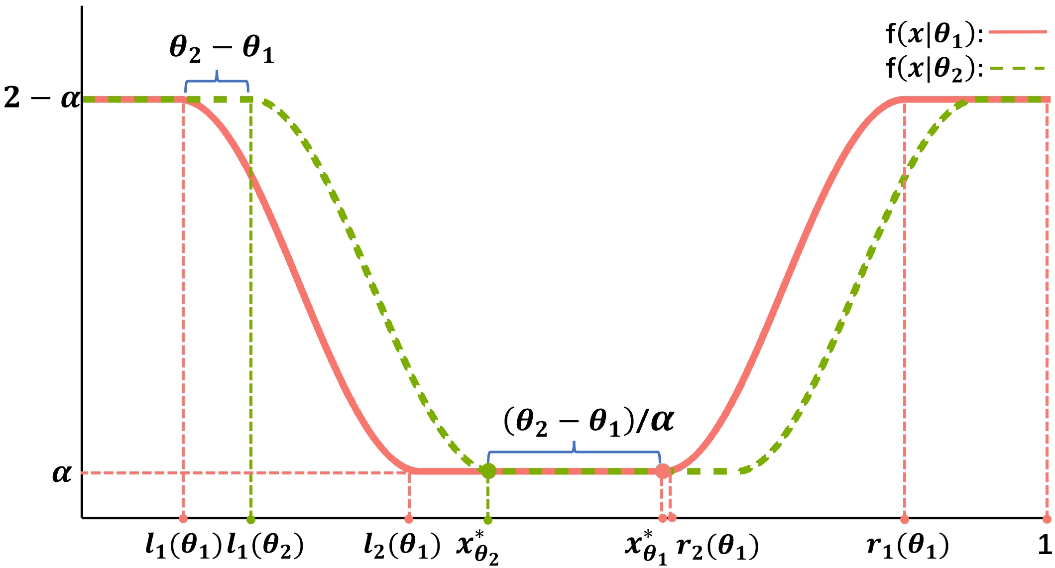
Figure 1: Our inverted-hat-shape hard instance using cosin functions to connect segments.

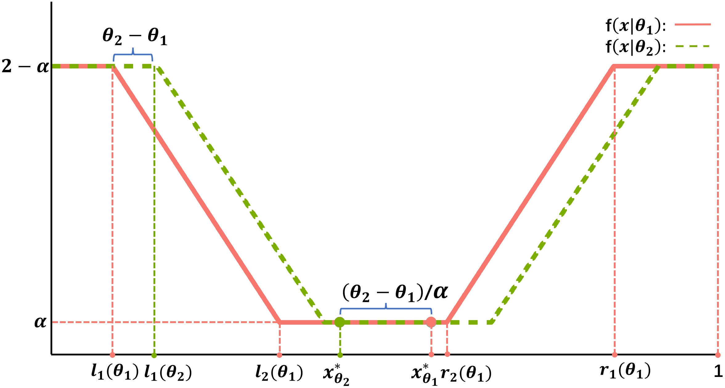
Figure 2: Another choice of hard instance using straight lines to connect segments.

The following lemma shows that our hard instance is well-defined and satisfies the basic assumptions.

Lemma 4.3

Suppose $\alpha\leq\min\left\{1/2,2\rho,2\left(1-\rho\right)\right\}$, $f(\cdot|\theta)$ is a well-defined PDF for any $\theta\in\Theta$, and our hard instance satisfies Assumptions A.1 – A.4.

Through the careful design of the inverted-hat-shape structure of the PDF plot in Figure 2, we can successfully constrain $x_{\theta}^{*}$ within the central part of the domain and thus make $x_{\theta}^{*}$ sensitive to parameter $\theta$. More specifically, as illustrated by Figure 2 and shown by the following lemma, our design guarantees that $x_{\theta}^{*}$ varies $\Omega(1)$ when $\theta$ varies only $\Theta(\alpha)$, which results in the relatively significant variability of $x_{\theta}^{*}$.

Lemma 4.4

For any $\theta\in\Theta:=[-\alpha/20,\alpha/20]$, we have $x_{\theta}^{*}$ lies within interval $[l_{2}(\theta),r_{2}(\theta)]$ and

$$x_{\theta}^{*}:=h(\theta)=\frac{\rho}{2}+\frac{4\rho-\alpha}{16-8\alpha}+\frac{1}{8}-\left(\frac{2}{\alpha}-2\right)\theta.$$ (8)

The following lemma demonstrates that the Fisher information of $f(\cdot|\theta)$ is bounded above by $\mathcal{O}(t)$.

Lemma 4.5

For any $t$ and $\theta\in\Theta:=[-\alpha/20,\alpha/20]$, the Fisher information

$$I_{t}(\theta):=\mathbb{E}_{\theta}\left[\left(\frac{\partial\log f\left(X_{1},\dots,X_{t}|\theta\right)}{\partial\theta}\right)^{2}\right]\leq\frac{4\pi^{2}t}{\rho(1-\rho)},$$ (9)

where $f\left(X_{1},\dots,X_{t}|\theta\right)$ is the joint PDF of independent random variables $X_{1}\dots X_{t}\sim f(\cdot|\theta)$, and $\mathbb{E}_{\theta}$ denotes the expectation over $X_{1},\dots,X_{t}$.

It is worth noting that in construction, we utilize the cosine functions to connect separated segments rather than employing simpler straight lines (see Figure 2). This approach is adopted because the Fisher information for the latter design is $\Theta(t\log 1/\alpha)$, as opposed to the desired $\mathcal{O}(t)$ in Lemma 4.5.

With all the above technical lemmas in hand, we are ready to complete the proof of Theorem 4.1.

Proof of Theorem 4.1. Since $\Theta=\left[-\alpha/20,\alpha/20\right]$, we have

$$\underset{\pi\in\Pi}{\inf}\underset{F\in\mathcal{F}_{\alpha}}{\sup}\{R^{\pi}\left(F,T\right)\}\geq\underset{\pi\in\Pi}{\inf}\int_{-\alpha/20}^{\alpha/20}\mathcal{R}^{\pi}(F_{\theta},T)q(\theta)\mathrm{d}\theta.$$ (10)

For an arbitrary policy $\pi$, by Eq. (7) the regret under the demand distribution $F_{\theta}$ is

$$\int_{-\alpha/20}^{\alpha/20}\mathcal{R}^{\pi}(F_{\theta},T)q(\theta)\mathrm{d}\theta\geq\sum_{t=1}^{T}\mathbb{E}\left[C_{\theta}\left(x_{t}^{\pi}\right)-C_{\theta}\left(x^{*}_{\theta}\right)\right]\geq\sum_{t=1}^{T}\frac{\left(\underset{x,\theta}{\min}C^{{}^{\prime\prime}}_{\theta}(x)/2\right)\mathbb{E}[h^{\prime}(\theta)^{2}]}{\mathbb{E}[I_{t}(\theta)]+I(q)},$$ (11)

Due to $f(x|\theta)\geq\alpha$, we have ${\min_{x,\theta}}C^{{}^{\prime\prime}}_{\theta}(x)\geq(h+b)\alpha$. By Lemma 4.4, we have $\mathbb{E}[h^{\prime}(\theta)^{2}]\geq(2/\alpha-2)^{2}$. Lemma 4.5 shows that $\mathbb{E}[I_{t}(\theta)]\leq 4\pi^{2}t/(\rho(1-\rho)).$ Besides, the Fisher information of $q(\theta)$ is

$$I(q)=\int_{-\alpha/20}^{\alpha/20}\frac{20^{3}\pi^{2}}{\alpha^{3}}\frac{\cos^{2}(10\pi\theta/\alpha)\sin^{2}(10\pi\theta/\alpha)}{\cos^{2}(10\pi\theta/\alpha)}\mathrm{d}\theta=\frac{400\pi^{2}}{\alpha^{2}}.$$ (12)

Therefore,

$$\underset{F\in\mathcal{F}_{\alpha}}{\sup}\{R^{\pi}\left(F,T\right)\} \geq\frac{(h+b)\alpha}{2}\sum_{t=1}^{T}\frac{2/\alpha-2}{4\pi^{2}t/(\rho(1-\rho))+400\pi^{2}/\alpha^{2}}$$

$$\geq\frac{h+b}{2\alpha}\sum_{t=1}^{T}\frac{\widetilde{K}_{6}}{t+\alpha^{-2}}\geq\frac{h+b}{2\alpha}\int_{1}^{T+1}\frac{\widetilde{K}_{6}}{t+\alpha^{-2}}\mathrm{d}t$$

$$\geq\frac{h+b}{2}\widetilde{K}_{6}\alpha^{-1}\ln\left(\frac{T+1+\alpha^{-2}}{1+\alpha^{-2}}\right)\geq\frac{h+b}{2}\widetilde{K}_{6}\alpha^{-1}(\ln T-2\ln\alpha^{-1}-\ln 2),$$

$$\geq C_{0}\alpha^{-1}\ln T,$$

where $\widetilde{K}_{6}=\min\{\rho(1-\rho)/4\pi^{2},1/(400\pi^{2})\}$, $K_{6}=\widetilde{K}_{6}(h+b)/12$, the second inequality is due to $\alpha\leq 1/2$ and the last inequality is due to $T\geq\max\{\alpha^{-3},64\}$.

5 Conclusion

In this paper, we close the regret gaps and establish the optimality of SAA under both global and local strong convexity conditions for data-driven newsvendor problems with general convex overage and underage cost. Our upper bound result demonstrates that the regret performance of SAA is only influenced by $\alpha$ in the long run under $(\alpha,\beta)$-local strong convexity. This insight enhances our understanding of how local properties affect the long-term regret performance of decision-making strategies. Our lower bound result is the first to match the existing upper bound with respect to both the parameter $\alpha$ and the time horizon $T$ simultaneously under $\alpha$-global strong convexity, which advances the theoretical understanding of the performance limit of data-driven methods in newsvendor problems. Moreover, the techniques we propose not only enrich the regret analysis techniques (including both upper bound and lower bound) in data-driven inventory management literature but also offer potential applications in broader data-driven decision-making problems.

6 Some Useful Technical Lemmas

By classic results and standard techniques in learning theory, we could translate pseudo-dimension into uniform convergence guarantees. For simplicity, we omit the definition of pseudo-dimension and the proof of the following lemma, please refer to Pollard (2012) for details.

Lemma 6.1

Let $\mathcal{F}$ be a $b$-uniformly bounded class, and let $\left\{X_{i}\right\}_{i=1}^{n}$ be a collection of i.i.d. samples from random variable $X$. For any positive integer $n\geq 1$ and any scalar $\delta\geq 0$, there exists a positive constant $C_{0}>0$ such that

$$\sup_{f\in\mathcal{F}}\left|\frac{1}{n}\sum_{i=1}^{n}f\left(X_{i}\right)-\mathbb{E}[f(X)]\right|\leq C_{0}b\sqrt{\frac{\mathrm{P}\text{-}\operatorname{dim}(\mathcal{F})}{N}}+\delta$$

with probability at least $1-\exp\left(-\frac{n\delta^{2}}{2b^{2}}\right)$, where $\mathrm{P}\text{-}\operatorname{dim}(\mathcal{F})$ is the pseudo dimension (or VC-subgraph dimension) of class $\mathcal{F}$.

Lemma 6.2 (The van Trees inequality (Gill and Levit 1995))

Let $(\mathcal{X},\mathcal{F},P_{\theta}:\theta\in\Theta,\mu)$ be a dominated family of distributions, where $\mathcal{X}$ is the sample space, $\mathcal{F}$ is the $\sigma$-algebra, $P_{\theta}$ is the probability measure with parameter $\theta$, the parameter space $\Theta$ is a closed interval on the real line, $\mu$ is the dominating measure. Let $f(x|\theta)$ denote the density of $P_{\theta}$ with respect to $\mu$, and $\pi$ be some probability distribution on $\Theta$ with a density $\lambda(\theta)$ with respect to the Lebesgue measure. Suppose the following assumptions hold:

1. $\lambda(\cdot)$ and $f(x|\cdot)$ are absolutely continuous ($\mu$-almost surely),

2. for any fixed $\theta\in\Theta$, $\mathbb{E}_{\theta}\left[\frac{\partial}{\partial\theta}\left(\log f\left(X|\theta\right)\right)\right]=0,$ where $\mathbb{E}_{\theta}$ denotes the expectation over $X\sim P_{\theta}$.

3. $\lambda(\cdot)$ converges to zero at the endpoints of the interval $\Theta$.

Let $\psi(\theta)$ be an absolute function. Then for any estimator $\widehat{\theta}(X)$ based on sample $X\sim P_{\theta}$, it holds that

$$\mathbb{E}\left[\left(\widehat{\psi}(x)-\psi(\theta)\right)^{2}\right]\geq\frac{\mathbb{E}[\psi^{\prime}(\theta)^{2}]}{\mathbb{E}\left[I(\theta)\right]+I\left(\lambda\right)},$$

where $\mathbb{E}$ denotes the expectation over the joint distribution of $X$ and $\theta$, $I(\theta)=\mathbb{E}_{\theta}\left[(\frac{\partial}{\partial\theta}\left(\log f\left(X|\theta\right)\right))^{2}\right]$ and $I(\lambda)=\mathbb{E}\left[(\frac{\partial}{\partial\theta}\left(\log\lambda(\theta)\right))^{2}\right]$ is the the Fisher information for $\theta$ and $\lambda$ respectively.

7 Omitted Proofs in Section 3

Proof of Lemma 3.3. By Assumption 3 and the definition of SAA, we know $|\widehat{g}_{t}(\widehat{x}_{t})|\leq C_{1}/\sqrt{t}$. Besides,

$$|g(\widehat{x}_{t})|\leq|g(\widehat{x}_{t})-\widehat{g}_{t}(x_{t})|+|\widehat{g}_{t}(\widehat{x}_{t})|\leq 2\sup_{x\in[0,\widebar{D}]}|\widehat{g}_{t}(x)-g(x)|+|\widehat{g}_{t}(\widehat{x}_{t})|.$$

We establish the concentration of $\sup_{x\in[0,\widebar{D}]}|\widehat{g}_{t}(x)-g(x)|$ by deriving the pseudo-dimension of the function class $\mathcal{F}=\{c^{\prime}(x,\cdot):x\in[0,\widebar{D}]\}$ and applying Lemma 6.1.

With a sight abuse of notation, we use $c^{\prime}(x,d)$ to refer the gradient (or subgradient) with respect to $x$. Given any demand samples $d_{1},d_{2},\dots,d_{m}$ and $\tau_{1},\tau_{2},\dots,\tau_{m}\in\mathbb{R}$, consider the set

$$S=\{(\mathbb{I}[c^{\prime}(x,d_{1})<\tau_{1}],\mathbb{I}[c^{\prime}(x,d_{2})<\tau_{2}],\dots,\mathbb{I}[c^{\prime}(x,d_{t})<\tau_{m}]):x\in[0,\widebar{D}]\}.$$

Since $c(x,d)$ is convex, $c^{\prime}(x,d)$ is non-decreasing in $x$ and the set $S$ has at most $m+1$ elements. It follows that the function class $\mathcal{F}=\{c^{\prime}(x,\cdot):x\in[0,\widebar{D}]\}$ has pseudo-dimension $m\leq 2$ (by $2^{m}\leq m+1$). Therefore, by Lemma 6.1, we know that with probability at least $1-\exp(-\frac{t\lambda^{2}}{2B^{2}})$,

$$\sup_{x\in[0,\widebar{D}]}|\widehat{g}_{t}(x)-g(x)|\leq\frac{\sqrt{2}C_{0}B}{\sqrt{t}}+\lambda,$$

where $B$ is the upper bound on $c^{\prime}(x,d)$ and $C_{0}$ is a universal constant in Lemma 6.1. Therefore, by the above discussion, we obtain

$$\mathbb{P}\left[\left|g(\widehat{x}_{t})\right|\geq\lambda+\frac{4C_{0}B+C_{1}}{\sqrt{t}}\right] \leq\mathbb{P}\left[2\sup_{x\in[0,\widebar{D}]}|\widehat{g}_{t}(x)-g(x)|+|\widehat{g}_{t}(\widehat{x}_{t})|\geq\lambda+\frac{2\sqrt{2}C_{0}B+C_{1}}{\sqrt{t}}\right]\leq\mathrm{exp}\left(-\frac{t\lambda^{2}}{2B^{2}}\right),$$

where the second inequality is due to $|\widehat{g}_{t}(\widehat{x}_{t})|\leq C_{1}/\sqrt{t}$.

8 Omitted Proofs in Section 4

Proof of Lemma 4.3. Since it is easy to verify the well-definiteness and Assumptions A.1 and A.2 for our hard instance. In the following, we verify Assumptions A.3 and A.4.

Verification of Assumption A.3. We will prove that the likelihood function $f(x|\cdot)$ is differentiable continuous, and consequently absolutely continuous. Fix $x\in[0,1]$, the likelihood function takes the following form

$$f(x|\theta)=\left\{\begin{aligned} &2-\alpha,&\theta\in((-\infty,\tilde{l}_{1}(x)]\cup[\tilde{r}_{1}(x),\infty))\cap\Theta,\\ &\alpha,&\theta\in[\tilde{l}_{2}(x),\tilde{r}_{2}(x)]\cap\Theta,\\ &\alpha+(1-\alpha)\left(\cos\left(w_{1}\left(\widetilde{r}_{1}(x)-\theta\right)\right)+1\right),&\theta\in[\widetilde{r}_{2}(x),\widetilde{r}_{1}(x)]\cap\Theta,\\ &\alpha+(1-\alpha)(\cos(w_{2}(\theta-\widetilde{l}_{1}(x)))+1),&\theta\in[\widetilde{l}_{1}(x),\widetilde{l}_{2}(x)]\cap\Theta,\end{aligned}\right.$$

where $\widetilde{l}_{1}(x)=x-(4\rho-\alpha)/(16-8\alpha)-3/4$, $\widetilde{l}_{2}(x)=x-(4\rho-\alpha)/(16-8\alpha)-1/4-\rho/2$, $\widetilde{r}_{2}(x)=x-(4\rho-\alpha)/(16-8\alpha)-\rho/2$, $\widetilde{r}_{1}(x)=x-(4\rho-\alpha)/(16-8\alpha)$, $w_{1}=2\pi/\rho$, and $w_{2}=2\pi/\left(1-\rho\right)$.

Through the above formulation, the derivative of the likelihood can be derived as

$$\frac{\mathrm{d}}{\mathrm{d}\theta}f(x|\theta)=\left\{\begin{aligned} &0,&\theta\in((-\infty,\tilde{l}_{1}(x)]\cup[\tilde{l}_{2}(x),\tilde{r}_{2}(x)]\cup[\tilde{r}_{1}(x),\infty))\cap\Theta,\\ &(1-\alpha)w_{1}\sin\left(w_{1}\left(\widetilde{r}_{1}(x)-\theta\right)\right),&\theta\in[\widetilde{r}_{2}(x),\widetilde{r}_{1}(x)]\cap\Theta,\\ &-(1-\alpha)w_{2}\sin\left(w_{2}\left(\theta-\widetilde{l}_{1}(x)\right)\right),&\theta\in[\widetilde{l}_{1}(x),\widetilde{l}_{2}(x)]\cap\Theta.\end{aligned}\right.$$

Thus, it is easy to note that for any $x\in[0,1]$, $f(x|\cdot)$ is absolutely continuous in $\Theta$.

Verification of Assumption A.4. Note that,

$$\mathbb{E}_{\theta}\left[\frac{\partial\log f\left(X|\theta\right)}{\partial\theta}\right]= \int_{l_{1}(\theta)}^{l_{2}(\theta)}(1-\alpha)w_{1}\sin\left(w_{1}\left(x-\frac{4\rho-\alpha}{16-8\alpha}-\theta\right)\right)\mathrm{d}x$$

$$-\int_{r_{2}(\theta)}^{r_{1}(\theta)}(1-\alpha)w_{2}\sin\left(w_{2}\left(\theta-x+\frac{3}{4}\right)\right)\mathrm{d}x.$$

Taking $y=w_{1}(x-l_{1}(\theta))$, $z=w_{2}(r_{1}(\theta)-x)$, by substituting the integral, one has

$$\int_{l_{1}(\theta)}^{l_{2}(\theta)}(1-\alpha)w_{1}\sin\left(w_{1}\left(x-\frac{4\rho-\alpha}{16-8\alpha}-\theta\right)\right)\mathrm{d}x=(1-\alpha)\int_{0}^{\pi}\sin\left(y\right)\mathrm{d}y=2(1-\alpha),$$

$$-\int_{r_{2}(\theta)}^{r_{1}(\theta)}(1-\alpha)w_{2}\sin\left(w_{2}\left(\theta-x+\frac{3}{4}\right)\right)\mathrm{d}x=-(1-\alpha)\int_{0}^{\pi}\sin\left(z\right)\mathrm{d}z=-2(1-\alpha).$$

Combining the above equations, we could get the conclusion.

Proof of Lemma 4.4. Let $F_{\theta}$ denote the cumulative distribution of $f(\cdot|\theta)$. For any $\theta\in\Theta$, since $-\alpha/16\leq\theta\leq\alpha/16$, it holds that

$$F_{\theta}\left(l_{2}(\theta)\right) =\int_{0}^{l_{1}(\theta)}f\left(x|\theta\right)\mathrm{d}x+\int_{l_{1}(\theta)}^{l_{2}(\theta)}f\left(x|\theta\right)\mathrm{d}x$$

$$=\left(2-\alpha\right)\left(\frac{4\rho-\alpha}{16-8\alpha}+\theta\right)+\frac{\rho}{2}\leq\rho-\frac{\alpha}{8}+\frac{\left(2-\alpha\right)\alpha}{16}<\rho.$$ (13)

Similarly, we have

$$F_{\theta}\left(r_{2}(\theta)\right) =\int_{0}^{l_{1}(\theta)}f\left(x|\theta\right)\mathrm{d}x+\int_{l_{1}(\theta)}^{l_{2}(\theta)}f\left(x|\theta\right)\mathrm{d}x+\int_{l_{2}(\theta)}^{r_{2}(\theta)}f\left(x|\theta\right)\mathrm{d}x$$

$$=\left(2-\alpha\right)\left(\frac{4\rho-\alpha}{16-8\alpha}+\theta\right)+\rho/2+\frac{\alpha}{4}=\rho+\frac{\alpha}{8}+\left(2-\alpha\right)\theta\geq\rho+\frac{\alpha}{8}-\frac{\left(2-\alpha\right)\alpha}{16}>\rho.$$ (14)

Combining Eq. (13) and Eq. (14), by definition of $x_{\theta}^{*}$, we have $\left[l_{2}(\theta),r_{2}(\theta)\right]$. Thus, solving equation

$$\rho=\int_{0}^{l_{1}(\theta)}f\left(x|\theta\right)\mathrm{d}x+\int_{l_{1}(\theta)}^{l_{2}(\theta)}f\left(x|\theta\right)\mathrm{d}x+\int_{l_{2}(\theta)}^{x_{\theta}^{*}}f\left(x|\theta\right)\mathrm{d}x=\left(2-\alpha\right)l_{1}(\theta)+\left(l_{2}(\theta)-l_{1}(\theta)\right)+\alpha\left(x_{\theta}^{*}-l_{2}(\theta)\right),$$

we obtain

$$x_{\theta}^{*}=\frac{\rho}{2}+\frac{4\rho-\alpha}{16-8\alpha}+\frac{1}{8}-\left(\frac{2}{\alpha}-2\right)\theta,$$

which completes the proof of this lemma.

Proof of Lemma 4.5. For any $t\geq 1$, let $I_{t}$ denote the expected Fisher information for $\theta$ at time $t$. It holds that,

$$I_{t}(\theta) =\mathbb{E}_{\theta}\left[\left(\frac{\partial\log f\left(X_{1},\dots,X_{t}|\theta\right)}{\partial\theta}\right)^{2}\right]$$

$$=\sum_{i=1}^{t}\mathbb{E}_{\theta}\left[\left(\frac{\partial\log f\left(X_{i}|\theta\right)}{\partial\theta}\right)^{2}\right]+2\sum_{1\leq i<j\leq t}\mathbb{E}_{\theta}\left[\frac{\partial\log f\left(X_{i}|\theta\right)}{\partial\theta}\right]\mathbb{E}_{\theta}\left[\frac{\partial\log f\left(X_{j}|\theta\right)}{\partial\theta}\right]=tI_{1}(\theta).$$ (15)

where the first equality is due to the independence of samples, and the second equality is due to Assumption A.4. Noting that $f(\cdot|\theta)$ is supported on $\left[0,1\right]$, we have

$$I_{1}(\theta) =\mathbb{E}_{\theta}\left[\left(\frac{\mathrm{d}}{\mathrm{d}\theta}\log f(x|\theta)\right)^{2}\right]=\int_{0}^{1}\frac{\left(\frac{\mathrm{d}}{\mathrm{d}\theta}f(x|\theta)\right)^{2}}{f(x|\theta)}\mathrm{d}x.$$

$$=\int_{l_{1}(\theta)}^{l_{2}(\theta)}\frac{(1-\alpha)^{2}w_{1}^{2}\sin^{2}\left(w_{1}\left(x-l_{1}(\theta)\right)\right)}{1+(1-\alpha)\cos\left(w_{1}\left(x-l_{1}(\theta)\right)\right)}\mathrm{d}x+\int_{r_{2}(\theta)}^{r_{1}(\theta)}\frac{(1-\alpha)^{2}w_{2}^{2}\sin^{2}\left(w_{2}\left(r_{1}(\theta)-x\right)\right)}{1+(1-\alpha)\cos\left(w_{2}\left(r_{1}(\theta)-x\right)\right)}\mathrm{d}x$$

$$=(1-\alpha)^{2}w_{1}\int_{0}^{\pi}\frac{1-\cos^{2}\left(y\right)}{1+(1-\alpha)\cos\left(y\right)}\mathrm{d}y+(1-\alpha)^{2}w_{2}\int_{0}^{\pi}\frac{1-\cos^{2}\left(z\right)}{1+(1-\alpha)\cos\left(z\right)}\mathrm{d}z,$$

where the last equality is due to $y=w_{1}(x-l_{1}(\theta))$, $z=w_{2}(r_{1}(\theta)-x)$ and bysubstitution of the integral. Since $1+(1-\alpha)\cos x>0$, and $1-\cos x\leq 2$ holds for any $x$, it is easy to calculate that

$$\frac{1-\cos^{2}(x)}{1+(1-\alpha)\cos(x)}\leq\frac{2\left(1+\cos(x)\right)}{1+(1-\alpha)\cos(x)}=\frac{2}{1-\alpha}\frac{(1-\alpha)\left(1+\cos(x)\right)}{\alpha+(1-\alpha)\left(1+\cos(x)\right)}\leq\frac{2}{1-\alpha},$$

and it follows that

$$I_{1}(\theta) =(1-\alpha)^{2}(w_{1}+w_{2})\int_{0}^{\pi}\frac{1-\cos^{2}(x)}{1+(1-\alpha)\cos(x)}\mathrm{d}x$$

$$\leq(1-\alpha)^{2}(w_{1}+w_{2})\int_{0}^{\pi}2(1-\alpha)^{-1}\mathrm{d}x=2\pi(1-\alpha)(w_{1}+w_{2}).$$

Combine this with Eq. (8), we get the conclusion that for any $\theta\in\Theta$, one has $I_{t}(\theta)=tI_{1}(\theta)\leq 2\pi(w_{1}+w_{2})t,$ where $w_{1}=2\pi/\rho$ and $w_{2}=2\pi/(1-\rho)$.

9 Constant Regret under Uniform Distributions

For the newsvendor problems with linear overage and underage costs (i.e., $c(x,d)=h\cdot(x-d)^{+}+b\cdot(d-x)^{+}$), Besbes and Muharremoglu (2013) proved the minimax lower bound under the global minimal separation (see their Theorem 1) by constructing a family of uniform distributions with CDF $F_{\theta},~{}\theta\in[0,1/2]$, where

$$F_{\theta}(x)=\left(x-\theta\right)\left(1-\theta\right)^{-1},\quad x\in[\theta,1].$$ (16)

Let $U(a,\widebar{b})$ denote the uniform distribution on $[a,\widebar{b}]$, and let $F_{a,\widebar{b}}$ be its CDF. We denote the uniform distribution family used in the proof of Theorem 1 in Besbes and Muharremoglu (2013) as $\mathcal{F}_{u}=\{F_{\theta,1}\mid\theta\in[0,1/2]\}.$

Next, we show that there exists a policy that can achieve constant regret under a uniform distribution. Specifically, we define $\rho=b/(h+b)$ and $\pi=(\pi_{t})_{t=1}^{T}$ as

$$\pi_{t}\left(D_{1},\dots,D_{t}\right)=\left(1-\rho\right)\min\left\{D_{1},\dots,D_{t}\right\}+\rho\max\left\{D_{1},\dots,D_{t}\right\},$$ (17)

where $D_{1},\dots,D_{t}$ are i.i.d. samples from $U(a,\widebar{b})$. Note that the policy $\pi$ is inspired by the maximum likelihood estimation of parameters $a,\widebar{b}$ for uniform distributions.

We have the following theorem on the performance of policy $\pi$.

Theorem D.1

For any fixed $a,\widebar{b}\in\mathbb{R}$, we have

$$\mathcal{R}^{\pi}\left(F_{a,\widebar{b}},T\right)\leq\left(\rho^{2}+\left(1-\rho\right)^{2}\right)(h+b)\left(\widebar{b}-a\right).$$

Proof D.2

Proof. Define $Y_{t}=\min\{D_{1},\dots,D_{t}\}$, $Z_{t}=\max\{D_{1},\dots,D_{t}\}$, then we know

$$\widehat{x}_{t}:=\pi_{t}\left(D_{1},\dots,D_{t}\right)=\left(1-\rho\right)Y_{t}+\rho Z_{t}.$$

When the demand distribution is $U(a,\widebar{b})$, we know the newsvendor solution is $x_{a,\widebar{b}}^{*}=\left(1-\rho\right)a+\rho\widebar{b}.$

Some calculation gives that $C^{\prime\prime}(x)=(h+b)/(\widebar{b}-a)$. Therefore, from the smoothness of $C(x)$, we have

$$C(\widehat{x}_{t})-C\left(x_{a,\widebar{b}}^{*}\right)\leq\frac{h+b}{2\left(\widebar{b}-a\right)}\left(\widehat{x}_{t}-x_{a,\widebar{b}}^{*}\right)^{2}.$$

It follows that

$$\mathcal{R}^{\pi}\left(F_{a,\widebar{b}},T\right) \leq\frac{h+b}{2(\widebar{b}-a)}\sum_{t=1}^{T}\mathbb{E}\left[\left(\widehat{x}_{t}-x_{a,\widebar{b}}^{*}\right)^{2}\right]$$

$$\leq\frac{h+b}{\widebar{b}-a}\sum_{t=1}^{T}\left(\left(1-\rho\right)^{2}\mathbb{E}\left[\left(Y_{t}-a\right)^{2}\right]+\rho^{2}\mathbb{E}\left[\left(Z_{t}-\widebar{b}\right)^{2}\right]\right).$$ (18)

Then we estimate the right-hand side terms of the above inequality.

$$\mathbb{E}\left[Y_{t}\right]=\int_{a}^{\widebar{b}}\frac{t}{\widebar{b}-a}\left(\frac{\widebar{b}-x}{\widebar{b}-a}\right)^{t-1}x\mathrm{d}x=a+\frac{\widebar{b}-a}{t+1},$$

$$\mathbb{E}\left[Y_{t}^{2}\right]=\frac{t}{\left(\widebar{b}-a\right)^{t}}\int_{a}^{\widebar{b}}\left(\widebar{b}-x\right)^{t-1}x^{2}\mathrm{d}x=a^{2}+\frac{2\left(\widebar{b}-a\right)}{t+1}\left(a+\frac{\widebar{b}-a}{t+2}\right).$$

Therefore, we get that

$$\mathbb{E}\left[\left(Y_{t}-a\right)^{2}\right]=\mathbb{E}\left[Y_{t}^{2}\right]+a^{2}-2a\mathbb{E}\left[Y_{t}\right]=\frac{2\left(\widebar{b}-a\right)^{2}}{\left(t+1\right)\left(t+2\right)}.$$

Similarly, we can show that

$$\mathbb{E}\left[\left(Z_{t}-\widebar{b}\right)^{2}\right]=\frac{2\left(\widebar{b}-a\right)^{2}}{\left(t+1\right)\left(t+2\right)}.$$

Combine the above equations with Eq. (18), we obtain

$$\mathcal{R}^{\pi}\left(F_{a,\widebar{b}},T\right) \leq\frac{h+b}{\widebar{b}-a}\sum_{t=1}^{T}\left(\left(1-\rho\right)^{2}\mathbb{E}\left[\left(Y_{t}-a\right)^{2}\right]+\rho^{2}\mathbb{E}\left[\left(Z_{t}-\widebar{b}\right)^{2}\right]\right)$$

$$\leq\frac{h+b}{\widebar{b}-a}\sum_{t=1}^{T}\left(\left(1-\rho\right)^{2}\frac{2\left(\widebar{b}-a\right)^{2}}{\left(t+1\right)\left(t+2\right)}+\rho^{2}\frac{2\left(\widebar{b}-a\right)^{2}}{\left(t+1\right)\left(t+2\right)}\right)$$

$$\leq\left(\rho^{2}+\left(1-\rho\right)^{2}\right)(h+b)\left(\widebar{b}-a\right),$$

where we complete the proof.

Then we have the following theorem about minimax regret over uniform distributions $\mathcal{F}_{u}$.

Theorem D.3

The minimax regret over $\mathcal{F}_{u}$ satisfies

$$\underset{\pi\in\Pi}{\inf}\underset{F\in\mathcal{F}_{u}}{\sup}\mathcal{R}^{\pi}(F,T)\leq\left(\rho^{2}+\left(1-\rho\right)^{2}\right)(h+b).$$

The above theorem contradicts the proof of Theorem 1 in Besbes and Muharremoglu (2013). We also find a subtle technical oversight in their lower bound proof which might be the cause of such a contradiction. Specifically, under their hard instance, the likelihood function $f(x|\cdot)$ is not continuous with respect to $\theta$, violating a necessary requirement for the applicability of the van Trees inequality (i.e., Assumption A.3, see Lemma 6.2 for details).

References

• Besbes and Mouchtaki (2023) Besbes O, Mouchtaki O (2023) How big should your data really be? data-driven newsvendor: Learning one sample at a time. Management Science 69(10):5848–5865.