Curie–Weiss Model under $\ell^{p}$ constraint and a Generalized Hubbard–Stratonovich Transform

Abstract.

We consider the Ising Curie–Weiss model on the complete graph constrained under a given $\ell_{p}$ norm for some $p>0$. For $p=\infty$, it reduces to the classical Ising Curie–Weiss model. We prove that for all $p>2$, there exists $\beta_{c}(p):=\frac{3}{p^{2/p}}\cdot\tfrac{\Gamma(1+1/p)}{\Gamma(1+3/p)}$ such that for $\beta<\beta_{c}(p)$, the magnetization is concentrated at zero and satisfies an appropriate Gaussian CLT; whereas for $\beta>\beta_{c}(p)$ the magnetization is not concentrated at zero similar to the classical case. Though $\beta_{c}(2)=1$, we have $\beta_{c}(p)>1$ for $p>2$ and $\lim_{p\to\infty}\beta_{c}(p)=3$. We further generalize the model for general symmetric spin distributions and prove a similar phase transition. For $0<p<1$, the log-partition function scales at the order of $n^{2/p-1}$. The proofs are mainly based on the generalized Hubbard–Stratonovich (GHS) transform, which is of independent interest.

1. Introduction

1.1. The Model

We consider the mean-field Curie–Weiss model under an $\ell^{p}$ constraint. The model has the same formula for the Hamiltonian and the Gibbs measure as in the classical Curie–Weiss model. However, the spins in this model are taken from the $n$-dimensional $\ell^{p}$-sphere instead of the hypercube as in the classical case. We fix a positive real number $p>0$ and define the spin configuration space $S_{n,p}$ to be the $n$-dimensional $\ell^{p}$-sphere of radius $n^{1/p}$, i.e.,

$$S_{n,p}:=\left\{\bm{\sigma}\in\mathds{R}^{n}\ \biggl{|}\ \frac{1}{n}\sum_{i=1}^{n}\left|\sigma_{i}\right|^{p}=1\right\}.$$

Consider the Gibbs measure at inverse temperature $\beta>0$ given by

$$d\mu_{n,\beta,p}(\bm{\sigma}):=\mathcal{Z}_{n,p}(\beta)^{-1}\exp(\beta H_{n}(\bm{\sigma}))\,d_{n,p}\bm{\sigma},$$ (1.1)

where $d_{n,p}$ is the uniform measure on $S_{n,p}$, $H_{n}(\bm{\sigma}):=\frac{1}{n}\sum_{i<j}\sigma_{i}\sigma_{j}$ is the Hamiltonian, and

$$\mathcal{Z}_{n,p}(\beta) :=\int_{S_{n,p}}\exp(\beta H_{n}(\bm{\sigma}))\,d_{n,p}\bm{\sigma}$$ (1.2)

is the partition function.

The classical Curie–Weiss model can be considered as the $p=\infty$ version of this model, where the critical inverse temperature is $\beta_{c}(\infty)=1$. When $p=2$, this model is equivalent to the self-scaled version with standard Gaussian base measure, and it is known that a similar phase transition happens at $\beta_{c}(2)=1$ (see Cerf and Gorny (2016); Gorny (2014) for more details at the critical $\beta_{c}(2)=1$).

1.2. Motivation

The classical Curie–Weiss model and its generalization by Ellis and Newman (1978) consider the product base measure, which leads to the independent structure. A natural question is whether there is a similar phase transition when the spin configuration has a dependence structure. In particular, in the $\ell^{p}$ constraint model, each spin has a global interaction with other spins and our question is whether there exists some $\beta_{c}(p)\in(0,\infty)$ such that for $\beta<\beta_{c}(p)$ the typical magnetization is concentrated at $0$ and for $\beta>\beta_{c}(p)$ it is not. From the explicit constraint model, our question is whether developing a general framework to analyze constrained spin models is possible.

The classical model can be understood as the special case $p=\infty$ in our model, and we are interested in the asymptotic behavior when $n$ goes to infinity. A natural question is whether the limits in $n$ and $p$ are interchangeable and whether there is a discontinuity. Specifically, we are interested in the behavior of the function $p\mapsto\beta_{c}(p)$ as $p$ varies from $0$ to $\infty$, for example, whether it is continuous and type of discontinuity if it is not. We clearly know that $\beta_{c}(2)=\beta_{c}(\infty)=1$. One might suspect that $\beta_{c}(p)$ is a constant or a continuous function for $p\in[2,\infty]$. However, the actual picture is quite involved and needs careful analysis.

Another motivation of the $\ell^{p}$-constraint model is the connection with the $\ell^{p}$-Gaussian Grothendieck problem. The $\ell^{p}$-Grothendieck problem is the optimization problem regarding the quadratic forms of a matrix over $\ell^{p}$. The corresponding disorder model of the $\ell^{p}$ Curie–Weiss model is closely related to the $\ell^{p}$-Grothendieck problem with a random matrix (see Chen and Sen (2023); Dominguez (2022); Khot and Naor (2012)).

1.3. Simplification

We can rewrite the model (1.1) with respect to a sequence of i.i.d. random variables to remove the dependency arising from the $\ell^{p}$ constraint, allowing us to generalize the model further. We define the norm $\left|\!\left|\!\left|\cdot\right|\!\right|\!\right|_{n,p}$ on $\mathds{R}^{n}$ as follows

$$\left|\!\left|\!\left|\bm{x}\right|\!\right|\!\right|_{n,p}:=\left(\frac{1}{n}\sum_{i=1}^{n}\left|x_{i}\right|^{p}\right)^{1/p}\text{ for }\bm{x}\in\mathds{R}^{n}.$$ (1.3)

Next, we define a collection of symmetric probability densities indexed by $p>0$ given by

$$\rho_{p}(x):=c_{p}\cdot e^{-\left|x\right|^{p}/p},\quad x\in\mathds{R}$$

where $c_{p}:=\frac{p^{-1/p}}{2\Gamma(1+1/p)}$ for $p>0$ and use $Z_{p}$ to denote a typical random variable having density $\rho_{p}$. Note that $|Z_{1}|\sim\text{Exp}(1)$ and $Z_{2}\sim\operatorname{N}(0,1)$. Moreover, it is easy to check that

$$\operatorname{\mathds{E}}\left|Z_{p}\right|^{p}=1\text{ for all }p>0.$$

One can easily verify that $\left|Z_{p}\right|^{p}/p$ is distributed as a Gamma random variable with shape parameter $1/p$ and scale parameter $1$, enabling us to compute all of its polynomial moments, in particular, the variance of $Z_{p}$ can be explicitly written as

$$\nu_{p}^{2}:=\operatorname{Var}(Z_{p})=\operatorname{\mathds{E}}Z_{p}^{2}=\frac{p^{2/p}\cdot\Gamma(1+3/p)}{3\Gamma(1+1/p)}\quad\text{ for }p>0.$$

Let the coordinates of the random vector $\bm{X}=(X_{1},X_{2},\ldots,X_{n})$ be $n$ i.i.d. random variables from $\rho_{p}$. Define

$$\widehat{X}_{i}:=\frac{X_{i}\;\;\;}{\left|\!\left|\!\left|\bm{X}\right|\!\right|\!\right|_{n,p}},\quad i=1,2,\ldots,n.$$

It is well-known (see Schechtman and Zinn (1990); Barthe et al. (2005)) that the vector $\widehat{\bm{X}}=(\widehat{X}_{1},\widehat{X}_{2},\ldots,\widehat{X}_{n})$ is uniformly distributed on the $n$-dimensional $\ell^{p}$-sphere $S_{n,p}$. In particular, for the partition function (1.2), we have

$$\mathcal{Z}_{n,p}(\beta) =\operatorname{\mathds{E}}\exp(\beta H_{n}(\widehat{\bm{X}}))$$

$$=\int_{\mathds{R}^{n}}\exp\left(\frac{\beta n}{2}\cdot\frac{\left|n^{-1}\sum_{i=1}^{n}x_{i}\right|^{2}}{\left|\!\left|\!\left|\bm{x}\right|\!\right|\!\right|_{n,p}^{2}}-\frac{\beta}{2}\cdot\frac{n^{-1}\sum_{i=1}^{n}x_{i}^{2}}{\left|\!\left|\!\left|\bm{x}\right|\!\right|\!\right|_{n,p}^{2}}\right)\prod_{i=1}^{n}\rho_{p}(x_{i})\,dx_{i}.$$ (1.4)

When $p\geqslant 1$, clearly

$$\frac{\left|n^{-1}\sum_{i=1}^{n}x_{i}\right|}{\left|\!\left|\!\left|\bm{x}\right|\!\right|\!\right|_{n,p}}\leqslant 1\text{ for all }\bm{x}\in\mathds{R}^{n}.$$

In particular, ${H_{n}(\bm{\sigma})}\leqslant n/2$ and for the log-partition function we get $\log\mathcal{Z}_{n,p}(\beta)\leqslant n\beta/2$ for all $\beta>0$. However, for $p\in(0,1)$ the Hamiltonian grows at the order of $n^{2/p-1}\gg n$ when finitely many of the spins are $\Theta(n^{1/p})$. The representation (1.3) also allows us to generalize the model further by replacing the base measure $\rho_{p}(x)dx$ with a general symmetric probability measure $d\rho(x)$; we postpone the discussion to Section 1.4.3.

By the strong law of large numbers, when $X_{1},X_{2},\ldots,X_{n}$ are i.i.d. from $\rho_{p}$, we have

$$\left|\!\left|\!\left|\bm{X}\right|\!\right|\!\right|_{n,p}^{p}\text{ is concentrated around }\operatorname{\mathds{E}}|X_{1}|^{p}=1\text{ for large }n.$$

Thus, motivated by the classical results by Ellis and Newman (1978), one expects the critical inverse temperature to be $\beta_{c}(p)$, where

$$\beta_{c}(p):=\nu_{p}^{-2}=\frac{3}{p^{2/p}}\cdot\frac{\Gamma(1+1/p)}{\Gamma(1+3/p)}$$ (1.5)

for $p\in[1,\infty)$. In Theorem 1.1 and Theorem 1.13, we prove that $\beta_{c}(p)$ is indeed the critical inverse temperature for the $\ell^{p}$ constraint Curie–Weiss model and its generalization to the $\ell^{p}$ self-scaled model (defined in Section 1.4.3) for $p\geqslant 2$. (See also Subsection 1.5.) Note that $\beta_{c}(2)$ coincides with the classical critical inverse temperature,i.e., $\beta_{c}(\infty)=1=\beta_{c}(2)$.

However, $\beta_{c}(p)$ converges to $3=1/\operatorname{Var}(U([-1,1]))$ as $p\to\infty$, which is different from $\beta_{c}(\infty)=1=1/\operatorname{Var}(U(\{+1,-1\}))$. Here, $U([-1,1])$ and $U(\{+1,-1\})$ are uniform distributions over $[-1,1]$ and $\{+1,-1\}$ respectively. This is due to the fact that $S_{n,p}$ can converge to the discrete hypercube or the continuous $\ell^{\infty}$-sphere depending on how we take the limit $p\to\infty$. For fixed $n$, if we take the limit $p\to\infty$ on the approximate constraint $\left(\sum_{i=1}^{n}|x_{i}|^{p}\right)^{1/p}\approx n^{1/p}$, then the limiting constraint defines the $\ell^{\infty}$-sphere $\{\bm{x}\in\mathds{R}^{n}:\max_{i}|x_{i}|\approx 1\}$. On the other hand, for fixed $n$ if we take the limit $p\to\infty$ on the exact constraint $\sum_{i=1}^{n}|x_{i}|^{p}=n$, then we obtain the discrete hypercube $\{\bm{x}\in\mathds{R}^{n}:\sum_{i=1}^{n}\lim_{p\to\infty}|x_{i}|^{p}=n\}=\{\bm{x}\in\mathds{R}^{n}:|x_{i}|=1\text{ for all }i=1,2,\cdots,n\}$. Here, we do not pursue a detailed analysis of the transition at $p=\infty$ and put it as an open question.

In analyzing the $\ell^{p}$ constraint model, the main difficulty is the nonlinearity arising from the $\ell^{p}$ scaling in the Gibbs measure and the Hamiltonian. In the classical case, one can linearize the quadratic terms in the Hamiltonian using the Hubbard–Stratonovich transform. Inspired by this, we develop a generalization of the transform by constructing an additive process that enables writing $Z\sim\rho_{p}$ as a product of independent random variables. It turns out that using the generalized Hubbard–Stratonovich (GHS) transform, one can linearize the Hamiltonian for computing the partition function and derive fluctuation of the magnetization and limiting free energy for $p\geqslant 2$.

1.4. Main Results

We first describe the main results before discussing the heuristics, background literature, and ideas behind the proofs.

1.4.1. $\ell^{p}$ constraint model

Our first main result is a phase transition of the Curie–Weiss model under $\ell^{p}$ constraint. Let $m_{n,\beta,p}(\bm{\sigma})=\frac{1}{n}\sum_{i=1}^{n}\sigma_{i}$ be the magnetization where $\bm{\sigma}$ is chosen according to the Gibbs measure (1.1) and $\beta_{c}(p)$ be defined as (1.5). The following theorem says that if $p\geqslant 2$, a phase transition of the magnetization $m_{n,\beta,p}$ happens at $\beta=\beta_{c}(p)$ and the fluctuation of $m_{n,\beta,p}$ is Gaussian as $n\to\infty$ when $\beta<\beta_{c}(p)$. Let

$$\psi_{p}(t):=\log\operatorname{\mathds{E}}[e^{tX}],\quad t\in\mathds{R}\,\text{ where }X\sim\rho_{p}.$$ (1.6)

Theorem 1.1.

Let $p\in[2,\infty)$ be fixed and $\beta_{c}(p)$ be as defined in (1.5). For all $\beta\geqslant 0$, we have

$$\lim_{n\to\infty}\frac{1}{n}\log\mathcal{Z}_{n,p}(\beta) =\sup_{z,w\geqslant 0}\left\{\psi_{p}\left(\sqrt{\beta}\frac{zw}{(1+z^{p})^{1/p}}\right)-\frac{1}{p}\log(1+z^{p})-\frac{p-2}{2p}w^{2p/(p-2)}\right\}$$ (1.7)

$$=\sup_{0\leqslant u<1,v\geqslant 0}\left\{\psi_{p}\left(\sqrt{\beta u^{2}v^{p-2}}\right)+\frac{1}{p}\log(1-u^{p})-\frac{p-2}{2p}v^{p}\right\}.$$

1. If $\beta<\beta_{c}(p)$, then $m_{n,\beta,p}$ is concentrated at zero and has a Gaussian limit as $n\to\infty$. More precisely, $\sqrt{n}\cdot m_{n,\beta,p}=\frac{1}{\sqrt{n}}\sum_{i=1}^{n}\sigma_{i}$ converges in distribution to $\mathrm{N}(0,(\beta_{c}(p)-\beta)^{-1})$ as $n\to\infty$ and $\mathcal{Z}_{n,p}(\beta)$ is uniformly bounded in $n$. In particular,

   $$\lim_{n\to\infty}\frac{1}{n}\log\mathcal{Z}_{n,p}(\beta)=0.$$

2. If $\beta>\beta_{c}(p)$, then $m_{n,\beta,p}$ is concentrated at $K\cup(-K)$ for some closed set $K\subset(0,1]$ and

   $$\lim_{n\to\infty}\frac{1}{n}\log\mathcal{Z}_{n,p}(\beta)>0.$$

The main tool used in the proof of Theorem 1.1 is the GHS transform introduced in the next Section 1.4.2. As an application of the GHS transform (see Lemma 2.1), we have for all $p\geqslant 2$,

$$\psi_{p}(t)\leqslant\psi_{2}(t\nu_{p})=t^{2}\nu_{p}^{2}/2,\qquad t\in\mathds{R}.$$

Using Young’s inequality $xy\leqslant\frac{2}{p}x^{p/2}+\frac{p-2}{p}y^{p/(p-2)}$ for $p>2,x,y\geqslant 0$, it is an easy exercise to see that for $\beta\leqslant\beta_{c}(p)=1/\nu_{p}^{2}$, we have

$$\psi_{p}\left(\sqrt{\beta u^{2}v^{p-2}}\right)+\frac{1}{p}\log(1-u^{p})-\frac{p-2}{2p}v^{p} \leqslant\frac{1}{2}u^{2}v^{p-2}+\frac{1}{p}\log(1-u^{p})-\frac{p-2}{2p}v^{p}$$

$$\leqslant\frac{1}{p}\log(1-u^{p})+\frac{1}{p}u^{p}\leqslant 0$$

for all $v\geqslant 0,u\in[0,1)$. It is nontrivial to show that the supremum in equation (1.7) is indeed strictly positive for $\beta>\beta_{c}(p)$. The proof is presented in Section 4.2.1.

Here, we note that the result in Theorem 1.1 cannot hold for $p<2$, as the right-hand side of equation 1.7 is infinity for $p<2$. However, in the $p>1$ case, we can use the theory of self-normalized processes (see de la Peña et al. (2009)) to get the following variational representation of the limiting free energy.

Proposition 1.2.

For $p>1$, we have

$$\lim_{n\to\infty}\frac{1}{n}\log\mathcal{Z}_{n,p}(\beta)$$

$$\qquad=\sup_{y,c\geqslant 0}\inf_{t\geqslant 0}\left\{\frac{\beta y^{2}}{2}+\psi_{p}\left(\frac{ct}{(1+ty)^{1/p}}\right)-\frac{1}{p}\log(1+ty)-\frac{p-1}{p}tyc^{p/(p-1)}\right\}.$$ (1.8)

For $p\neq 2$, the right-hand side of equation (1.2) in Proposition 1.2 can be written in a way similar to equation (1.7). By doing a change of variables, $w=(\beta y^{2})^{1/2-1/p},z=(\beta y^{2})^{1/p}c^{-1/(p-1)},t=s\cdot z^{p}/y$, we get

$$\lim_{n\to\infty}\frac{1}{n}\log\mathcal{Z}_{n,p}(\beta)$$

$$\qquad=\sup_{z,w\geqslant 0}\inf_{s\geqslant 0}\left\{\psi_{p}\left(\frac{\sqrt{\beta}\cdot szw}{(1+sz^{p})^{1/p}}\right)-\frac{1}{p}\log(1+sz^{p})-\frac{2ps-2s-p}{2p}w^{2p/(p-2)}\right\}.$$

By taking $s=1$, we thus get for $p>1$,

$$\lim_{n\to\infty}\frac{1}{n}\log\mathcal{Z}_{n,p}(\beta)\leqslant\sup_{z,w\geqslant 0}\left\{\psi_{p}\left(\frac{\sqrt{\beta}\cdot zw}{(1+z^{p})^{1/p}}\right)-\frac{1}{p}\log(1+z^{p})+\frac{2-p}{2p}w^{2p/(p-2)}\right\}.$$

For $p\in(1,2)$, we can use the GHS transform to get the following result. Since it follows from Theorem 1.13 with a change of variables, we omit the proof.

Theorem 1.3.

Let $p\in(1,2)$ be fixed and $E_{p}(\beta):=\lim_{n\to\infty}\frac{1}{n}\log\mathcal{Z}_{n,p}(\beta)$ for $\beta\geqslant 0$. We have

$$\sup_{z\geqslant 0}\left(\psi_{p}(\sqrt{y}z/(1+|z|^{p})^{1/p})-\frac{1}{p}\log(1+|z|^{p})\right)=\sup_{x\geqslant 0}\left\{E_{p}(xy)-\frac{2-p}{2p}x^{\frac{p}{2-p}}\right\}.$$

In particular, we have

$$\lim_{n\to\infty}\frac{1}{n}\log\mathcal{Z}_{n,p}(\beta)\leqslant\inf_{w>0}\sup_{z\geqslant 0}\left\{\psi_{p}\left(\frac{\sqrt{\beta}\cdot zw}{(1+z^{p})^{1/p}}\right)-\frac{1}{p}\log(1+|z|^{p})+\frac{2-p}{2p}w^{\frac{2p}{p-2}}\right\}.$$ (1.9)

Remark 1.4.

Note that the right-hand side of (1.9) is not a convex function of $\beta$, in general, because it is defined by an infimum of convex functions. Since the limiting free energy is convex in $\beta$, the inequality (1.9) may not be a tight bound for the limiting free energy. Proposition 1.2 tells us that the log-partition function converges as $n\to\infty$ to a well-defined function of $\beta$. However, the limit is given by supremum and infimum over three variables, so the variational formula does not give us much information about the phase transition and the critical temperature. It is open to find a variational formula for the limiting free energy similar to the $p\geqslant 2$ case and the critical temperature for $1<p<2$. We believe that similar to the $p\geqslant 2$ case, a phase transition happens in the $p\in(1,2)$ case at $\beta=\beta_{c}(p)$.

In the case when $0<p<1$, the log-partition function has a super-linear scaling, and the limiting free energy is an explicit function of $p$.

Theorem 1.5.

Define $p_{1}:=0$ and $p_{k}:=\frac{2\log(1+1/k)}{\log(1+2/(k-1))}$ for $k\geqslant 2$. For $p\in(p_{k-1},p_{k}]$, define $\tau(p):=k^{1-2/p}\cdot(k-1)$. For $p\in(0,1)$, we have

$$\lim_{n\to\infty}n^{1-2/p}\log\mathcal{Z}_{n,p}(\beta)=\frac{\beta}{2}\tau(p).$$

The result follows from Theorem 1.14 as a particular case because $X\sim\rho_{p}$ satisfies the both assumptions. Indeed, since $\mathbb{P}(|X|<x)\geqslant Ce^{-|x|^{p}/p}$, $\rho_{p}$ satisfies Assumption (2.). Thus we omit the proof.

1.4.2. Generalized Hubbard–Stratonovich transform

The following result plays a crucial role in analyzing the $\ell_{p}$ constraint Curie–Weiss model. The phase transition and the Gaussian fluctuation of the classical Curie–Weiss model can be investigated by the Hubbard–Stratonovich transform, which enables us to linearize the Hamiltonian (see Section 1.7). It turned out that we can use the following generalized version of the Hubbard–Stratonovich (GHS) transform to linearize the $\ell^{p}$ self-scaled Hamiltonian in our model.

Theorem 1.6 (GHS transform).

For any $p\geqslant 2$, there exists a positive r.v. $U=U_{2,p}$, such that for all $x\in\mathds{R},y>0$ we have

$$y^{-1/p}\exp\left(x^{2}y^{-2/p}\right)=c_{p}\cdot\operatorname{\mathds{E}}_{U}\int_{\mathds{R}}e^{\sqrt{2}xzU-y\left|z\right|^{p}/p}\,dz$$

where $c_{p}=\frac{p^{-1/p}}{2\Gamma(1+1/p)}$.

Corollary 1.7.

In particular, for $(\omega_{i},\nu_{i})_{i\geqslant 1}$ i.i.d. random vectors with $\nu_{1}>0$ a.s. and $p\geqslant 2$, we have

$$\operatorname{\mathds{E}}\left[\biggl{(}\frac{1}{n}\sum_{i=1}^{n}\nu_{i}\biggr{)}^{-1/p}\exp\left(\frac{\beta}{2n}\biggl{(}\sum_{i=1}^{n}\omega_{i}\biggr{)}^{2}\biggl{(}\frac{1}{n}\sum_{i=1}^{n}\nu_{i}\biggr{)}^{-2/p}\right)\right]$$

$$\qquad\qquad=c_{p}\cdot\operatorname{\mathds{E}}_{U}\int_{\mathds{R}}\left(\operatorname{\mathds{E}}\exp\left(\sqrt{\frac{\beta}{n}}\cdot\omega_{1}zU-\frac{\nu_{1}}{n}\cdot\frac{1}{p}\left|z\right|^{p}\right)\right)^{n}\,dz.$$

The key ingredient of the GHS transform is the existence of a positive random variable $U$ independent of $X\sim\rho_{p}$, $p\geqslant 2$, satisfying $X\cdot U\sim\mathrm{N}(0,1)=\rho_{2}$. Indeed, we construct a stochastic process $U_{p,q}$ indexed by $0<p<q$ such that $Z_{p}\cdot U_{p,q}\sim\rho_{q}$ where $Z_{p}\sim\rho_{p}$. The proof is based on the following construction of an additive process.

Theorem 1.8.

There exists an additive process $(Y_{t})_{t>0}$ with independent increments such that $Y_{t}\stackrel{{\scriptstyle\mathrm{d}}}{{=}}t\log X_{t}$ and $X_{t}\sim\textsc{Gamma}(t,1)$ for all $t>0$. Moreover, $Y_{0}\sim-\textsc{Exp}(1)$.

By Theorem 1.8 and letting $U_{p_{1},p_{2}}\stackrel{{\scriptstyle\mathrm{d}}}{{=}}\exp(Y_{1/p_{1}}-Y_{1/p_{2}})$, one can show the following.

Proposition 1.9.

Let $Z_{p}\sim\rho_{p}$ for $p>0$. For every $0<q<p$, there exists a positive r.v. $U=U_{p,q}$ independent of $Z_{p}$ such that

$$Z_{p}\cdot U_{p,q}\stackrel{{\scriptstyle\mathrm{d}}}{{=}}Z_{q}.$$

Moreover, $U_{p,q}$ has a strictly positive density $\theta_{p,q}(\cdot)$ on $(0,\infty)$ which satisfies

$$\lim_{x\to\infty}x^{-pq/(p-q)}\log\theta_{p,q}(x)=-\frac{p-q}{pq}.$$

Proposition 1.9 says that a random variable $Z_{q}$ can be written as a product of independent random variables. It is well-known (see Dufresne (2010) for example) that there are various identities regarding families of Beta and Gamma random variables, for example,

$$G^{(a)}+G^{(b)}=G^{(a+b)},\qquad B^{(a,b)}G^{(a+b)}=G^{(a)}$$

where $G^{(a)}$ is a Gamma random variable with the shape parameter $a$ and the scale parameter 1, and $B^{(a,b)}$ is a Beta random variable with parameters $a,b$. This is the so-called beta-gamma algebra. Since the $p$-th power of $Z_{p}\sim\rho_{p}$ is Gamma, the proposition can be understood as a variant of the beta-gamma algebra for the powers of Gamma distributions.

For general $p>2$, using Mellin transform, we show that the random variable $U_{2,p}$ has density $\theta_{p}$ where

$$\theta_{p}(x):=\frac{\Gamma(1/p)}{2\pi\Gamma(1/2)}\cdot\int_{\mathds{R}}x^{-it}\cdot\frac{\Gamma((1+it)/2)}{\Gamma((1+it)/p)}\,dt,\text{ for }x>0.$$

Moreover, for $a>0$, we have

$$\left|\frac{\Gamma(a+ib)}{\Gamma(a)}\right|=\prod_{k=0}^{\infty}\left(1+b^{2}/(a+k)^{2}\right)^{-1/2}\approx\exp(-b^{2}/2a),$$

which implies that $\theta_{p}$ is well-defined for $p>2$. The rigorous argument can be found in Section 3.3 in the proof of Proposition 1.9.

Remark 1.10.

In the case of $p=4$, one can explicitly compute the density of $U_{2,4}$ such that $U_{2,4}\cdot Z_{4}\sim\operatorname{N}(0,1)$, where $Z_{4}\sim\rho_{4}$ with

$$\rho_{4}(x)=\frac{\sqrt{2}}{\Gamma(1/4)}\cdot\exp(-x^{4}/4),\qquad x\in\mathds{R}.$$

Let $\theta_{2,4}:[0,\infty)\to\mathds{R}$ be the density given by

$$\theta_{2,4}(u):=\frac{1}{\sqrt{2}\Gamma(3/4)}\cdot u^{2}\exp(-u^{4}/4),\qquad u>0.$$

One can check that if $\theta_{2,4}$ is the density of $U_{2,4}$ and $U\perp Z_{4}$, then $U_{2,4}\cdot Z_{4}\sim\operatorname{N}(0,1)$.

In the proofs of the main results, we mainly used the existence of a random variable $U_{p,2}$ independent of $Z_{p}$ in Proposition 1.9 that satisfies $Z_{p}U_{p,2}\stackrel{{\scriptstyle\mathrm{d}}}{{=}}Z_{2}$, whereas we indeed constructed a stochastic process $U_{p,q}$ in $p$ for fixed $q$ in Theorem 1.8. A geometric interpretation and other possible applications of this stochastic process are of independent interest.

1.4.3. The $\ell^{p}$ self-scaled model

One can generalize the $\ell^{p}$ constraint model to the $\ell^{p}$ self-scaled model. As we have seen, the $\ell^{p}$ constraint Curie–Weiss model can be written in terms of self-normalized process $\widehat{\bm{X}}=(\widehat{X}_{1},\widehat{X}_{2},\ldots,\widehat{X}_{n})$ where

$$\widehat{X}_{i}:=\frac{X_{i}\;\;\;}{\left|\!\left|\!\left|\bm{X}\right|\!\right|\!\right|_{n,p}},\quad i=1,2,\ldots,n,$$

and the random vector $\bm{X}=(X_{1},X_{2},\ldots,X_{n})$ be $n$ i.i.d. random variables from $\rho_{p}$. Motivated by (1.3), one can consider $\ell^{p}$ self-scaled model with a symmetric base measure $\rho$, defined by

$$\mathcal{Z}_{n,p}(\beta;\rho) =\operatorname{\mathds{E}}\left[\frac{\beta}{n}\cdot\frac{\sum_{i<j}X_{i}X_{j}}{\left|\!\left|\!\left|\bm{X}\right|\!\right|\!\right|^{2}_{n,p}}\right]$$

$$=\int_{\mathds{R}^{n}}\exp\left(\frac{\beta n}{2}\cdot\frac{\left|n^{-1}\sum_{i=1}^{n}x_{i}\right|^{2}}{\left|\!\left|\!\left|\bm{x}\right|\!\right|\!\right|_{n,p}^{2}}-\frac{\beta}{2}\cdot\frac{n^{-1}\sum_{i=1}^{n}x_{i}^{2}}{\left|\!\left|\!\left|\bm{x}\right|\!\right|\!\right|_{n,p}^{2}}\right)\prod_{i=1}^{n}d\rho(x_{i}).$$

The above $\ell^{p}$ constraint model can be generalized with respect to any symmetric base measure $\rho$ on $\mathds{R}$ with $\mathbb{P}(X=0)=0$, $X\sim\rho$, and finite $p$-th moment under the self-scaled Hamiltonian

$$H_{n,p}(\bm{x}):=\frac{n}{2}\cdot\frac{\left|n^{-1}\sum_{i=1}^{n}x_{i}\right|^{2}}{\left|\!\left|\!\left|\bm{x}\right|\!\right|\!\right|_{n,p}^{2}}-\frac{1}{2}\cdot\frac{n^{-1}\sum_{i=1}^{n}x_{i}^{2}}{\left|\!\left|\!\left|\bm{x}\right|\!\right|\!\right|_{n,p}^{2}}.$$

Assumption 1.11.

Let $X\sim\rho$ with $\operatorname{\mathds{E}}_{\rho}|X|^{p}=1$. In what follows, we assume one of the following:

1. $\operatorname{\mathds{P}}(|X|>0)=1$ and $\operatorname{\mathds{E}}_{\rho}e^{\theta|X|^{p}}<\infty$ for some $\theta>0$.

2. $\operatorname{\mathds{P}}(|X|>0)=1$ and $\operatorname{\mathds{E}}_{\rho}[|X|^{-\alpha}]<\infty$ for some $\alpha>0$.

Since the Hamiltonian is normalized in the $\ell^{p}$ norm, it is necessary to assume that the base measure $\rho$ does not give a mass at 0 and decays fast enough near 0. Note that for $\rho_{p}$ distribution, Assumption (B) holds for any $0<\alpha<1$. For Assumption (A), one can find the same condition in Ellis and Newman (1978), where the generalized Curie–Weiss model was investigated.

Note that Assumption (A) is stronger than Assumption (B) and is needed only for the large deviation argument (Theorem 1.12). Using the GHS transform, we obtain a simpler variational form of the limiting free energy (Theorem 1.13) only under Assumption (B).

Large deviation based analysis. We write $\mathcal{Z}_{n,p}(\beta;\rho)$ to denote the corresponding partition function with $\sigma_{i},i\in[n]$ being i.i.d. from $\rho$. That is,

$$\mathcal{Z}_{n,p}(\beta;\rho)=\int_{\mathds{R}^{n}}\exp\left(\frac{\beta n}{2}\cdot\frac{\left|n^{-1}\sum_{i=1}^{n}x_{i}\right|^{2}}{\left|\!\left|\!\left|\bm{x}\right|\!\right|\!\right|_{n,p}^{2}}-\frac{\beta}{2}\cdot\frac{n^{-1}\sum_{i=1}^{n}x_{i}^{2}}{\left|\!\left|\!\left|\bm{x}\right|\!\right|\!\right|_{n,p}^{2}}\right)\prod_{i=1}^{n}d\rho(x_{i}).$$

Since

$$\frac{n^{-1}\sum_{i=1}^{n}x_{i}^{2}}{\left|\!\left|\!\left|\bm{x}\right|\!\right|\!\right|_{n,p}^{2}}\leqslant\begin{cases}1,&p\geqslant 2,\\ n^{\tfrac{2}{p}-1},&1<p<2,\end{cases}=o(n)\text{ for }p>1,$$

it suffices to consider the following partition function

$$\widetilde{\mathcal{Z}}_{n,p}(\beta;\rho)=\int_{\mathds{R}^{n}}\exp\left(\frac{\beta n}{2}\cdot\frac{\left|n^{-1}\sum_{i=1}^{n}x_{i}\right|^{2}}{\left|\!\left|\!\left|\bm{x}\right|\!\right|\!\right|_{n,p}^{2}}\right)\prod_{i=1}^{n}d\rho(x_{i}).$$ (1.10)

Let $F(x,y)=\frac{\beta}{2}x^{2}y^{-2/p}$ and $\mathcal{X}:=\{(x,y)\in\mathds{R}^{2}:0\leqslant|x|\leqslant y^{1/p}\}$. Let $(X_{i})_{i\geqslant 1}$ be an i.i.d. sequence of random variables with density $\rho$, $S_{n}=\sum_{i=1}^{n}X_{i}$, and $T_{n}=\sum_{i=1}^{n}|X_{i}|^{p}$. Let $Q_{n}$ be the joint distribution of $(S_{n}/n,T_{n}/n)$. The log Laplacian and the Cramér transform of $(X,|X|^{p})$ are given by

$$\psi_{\rho}(u,v):=\log\operatorname{\mathds{E}}_{\rho}e^{uX+v|X|^{p}},\qquad I(x,y):=\sup_{u,v}(ux+vy-\psi_{\rho}(u,v)).$$

Then, the partition function $\widetilde{\mathcal{Z}}_{n,p}(\beta;\rho)$ can be written as

$$\widetilde{\mathcal{Z}}_{n,p}(\beta;\rho)=\int_{\mathcal{X}}e^{nF(x,y)}Q_{n}(dx,dy).$$

Let $Q_{n,F}(A)=\widetilde{\mathcal{Z}}_{n,p}(\beta;\rho)^{-1}\int_{A}e^{nF}dQ_{n}$. We refer to the book Dembo and Zeitouni (2010) for detailed discussions on large deviation principles.

Theorem 1.12.

Let $X\sim\rho$ with $\operatorname{\mathds{E}}_{\rho}|X|^{p}=1$ and $p\geqslant 1$ be fixed. Assume that Assumption (A) holds. Then, $\{Q_{n,F}\}_{n\geqslant 1}$ has a large deviation property with speed $n$ and a rate function $I_{F}(x,y):=I(x,y)-F(x,y)$ and

$$\lim_{n\to\infty}\frac{1}{n}\log\mathcal{Z}_{n,p}(\beta;\rho)=\sup_{0\leqslant|x|\leqslant y^{1/p}}\left(F(x,y)-I(x,y)\right).$$ (1.11)

Furthermore, if $K$ is a closed subset in $\mathds{R}^{2}$ that does not contain any minimum points of $I_{F}$, then $Q_{n,F}(K)\leqslant e^{-Cn}$ for large $n$ and some constant $C=C(K)>0$.

Analysis using Generalized Hubbard–Stratonovich Transform. For $X\sim\rho_{p}$, it is easy to check that

$$\sup_{0\leqslant|x|\leqslant y^{1/p}} \left(\frac{1}{2}\beta x^{2}y^{-2/p}-I(x,y)\right)$$

$$=\sup_{0\leqslant x\leqslant y^{1/p}}\inf_{u,v}\left(\frac{1}{2}\beta x^{2}y^{-2/p}+\log\operatorname{\mathds{E}}_{\rho}e^{uX+v|X|^{p}}-ux-vy\right)$$

$$\leqslant\sup_{z,w\geqslant 0}\left(\log\operatorname{\mathds{E}}_{\rho}e^{\sqrt{\beta}zwX-|zX|^{p}/p}-\frac{p-2}{2p}\cdot w^{2p/(p-2)}\right)$$

by taking

$$u=\sqrt{\beta}zw,v=-z^{p}/p\text{ where }x=w^{2p/(p-2)}/(\sqrt{\beta}zw),y=w^{2p/(p-2)}/z^{p}.$$

It turns out that the equality holds under a weaker assumption on $\rho$.

Theorem 1.13.

Let $X\sim\rho$ with $\operatorname{\mathds{E}}_{\rho}|X|^{p}=1$ and Assumption (B) holds.

1. If $p>2$, then

   $$\lim_{n\to\infty}\frac{1}{n}\log\mathcal{Z}_{n,p}(\beta;\rho)=\sup_{z,w\geqslant 0}\left\{\psi_{\rho}(\sqrt{\beta}zw,-|z|^{p}/p)-\frac{p-2}{2p}\cdot w^{\frac{2p}{p-2}}\right\}.$$ (1.12)

   Furthermore, the limit is strictly positive if $\beta>\beta_{c}(\rho):=1/\operatorname{\mathds{E}}_{\rho}[X^{2}]$ and $0$ if $\beta\leqslant 1$.

2. For $p=2$, we have

   $$\lim_{n\to\infty}\frac{1}{n}\log\mathcal{Z}_{n,2}(\beta;\rho)=\sup_{z\geqslant 0}\psi_{\rho}(\sqrt{\beta}z,-z^{2}/2).$$

   Furthermore, the limit is strictly positive for $\beta>\beta_{c}(\rho)$, and the limit is zero for $\beta<\beta_{c}(\rho)$.

3. If $1<p<2$, then

   $$E(\beta) :=\lim_{n\to\infty}\frac{1}{n}\log\mathcal{Z}_{n,p}(\beta;\rho)=\sup_{y,c\geqslant 0}\inf_{t\geqslant 0}\left\{\frac{1}{2}\beta y^{2}+\psi_{\rho}\left(ct,-ty/p\right)-\frac{p-1}{p}tyc^{p/(p-1)}\right\}$$

   and

   $$\sup_{z\geqslant 0}\psi_{\rho}(\sqrt{y}z,-|z|^{p}/p)=\sup_{x\geqslant 0}\left\{E(xy)-\frac{2-p}{2p}x^{\frac{p}{2-p}}\right\}.$$

   In particular,

   $$\lim_{n\to\infty}\frac{1}{n}\log\mathcal{Z}_{n,p}(\beta;\rho)\leqslant\inf_{w>0}\sup_{z\geqslant 0}\left\{\psi_{\rho}\left({\sqrt{\beta}zw},-|z|^{p}/p\right)-\frac{p-2}{2p}w^{\frac{2p}{p-2}}\right\}.$$

Note that the representation (1.12) for $p>2$ case is a generalization of (1.14) in the classical Curie–Weiss model. One can prove a Gaussian CLT for the scaled magnetization in the setting of Theorem 1.13 for $\beta<1,p>2$ case. It is interesting to see if the maximizers in the right-hand side of (1.12) give us the information of the concentration of the magnetization as the large deviation results do in Theorem 1.12 for all $\beta<\beta_{c}(\rho)$.

For $p\in(0,1)$, we generalize the results in Theorem 1.5 to the $\ell^{p}$ self-scaled model as follows.

Theorem 1.14.

Let $(p_{k})_{k\geqslant 1}$ and the function $\tau(\cdot)$ be as defined in Theorem 1.5. Assume that for $X\sim\rho$, $\mathbb{P}(X=0)=0$, and one of the following holds:

1. $|\log\mathbb{P}(x\leqslant X\leqslant tx)|\leqslant Cx^{\alpha_{1}}$ for $C>0$, $x\to\infty$, $t\downarrow 1$, and $\alpha_{1}<2-p$.

2. $|\log\mathbb{P}(|X|<x)|\leqslant Cx^{-\alpha_{2}}$ for $C>0$, $x\to 0$, and $\alpha_{2}<2(1-p)$.

For $p\in(0,1)$, we have

$$\lim_{n\to\infty}n^{1-2/p}\log\mathcal{Z}_{n,p}(\beta;\rho)=\frac{\beta}{2}\tau(p).$$

1.5. Discussion on the Critical Temperatures

In Theorem 1.1, we have seen that the $\ell^{p}$ constraint Curie–Weiss model for $p>2$ has the critical inverse temperature $\beta_{c}(p)$ as in (1.5) in a sense that if $\beta<\beta_{c}(p)$ then the limiting free energy

$$\lim_{n\to\infty}\frac{1}{n}\log\mathcal{Z}_{n,p}(\beta)=0$$

and for $\beta>\beta_{c}(p)$ then the limiting free energy is strictly positive.

In the $\ell^{p}$ self-scaled model with general base measure $\rho$, Theorem 1.13 (a) tells us that the limiting free energy is strictly positive when $\beta>\beta_{c}(\rho):=1/\operatorname{Var}_{\rho}(X)$. However, it is unclear that $\beta_{c}(\rho)$ is indeed the critical inverse temperature. To show this, it follows from (1.12) that we need to show

$$\operatorname{\mathds{E}}\exp\left(\sqrt{\beta}zwX-z^{p}|X|^{p}/p\right)\leqslant\exp\left(\frac{p-2}{2p}w^{2p/(p-2)}\right)$$ (1.13)

for all $z,w\geqslant 0,\beta\leqslant\beta_{c}(\rho)$, where $X\sim\rho$.

One can derive the inequality for $\rho=\rho_{p}$, as mentioned in the discussion after Theorem 1.1.The inequality (1.13) holds true for $\rho=\frac{1}{2}\delta_{1}+\frac{1}{2}\delta_{-1}$ as well. Indeed,

$$\psi_{\rho}(\sqrt{\beta_{c}(\rho)}zw,-z^{p}/p) =\operatorname{\mathds{E}}_{\rho}\exp\left(\sqrt{\beta_{c}(\rho)}zwX-z^{p}|X|^{p}/p\right)$$

$$=\cosh(zw)e^{-z^{p}/p}\leqslant\exp\left(\frac{z^{2}w^{2}}{2}-\frac{z^{p}}{p}\right)\leqslant\exp\left(\frac{p-2}{2p}w^{2p/(p-2)}\right).$$

Here, we used the bound $\cosh(t)\leqslant\exp(t^{2}/2)$ and Young’s inequality $ab\leqslant a^{q}/q+b^{r}/r$ for $q=p/2$ and $1/q+1/r=1$. The inequality (1.13) is open for general symmetric measures. Note that one can show (1.13) for $\beta\leqslant 1$ using Young’s inequality.

For $p=2$ case, Theorem 1.13 (b) shows that $\beta_{c}(\rho)$ is the critical inverse temperature for the $\ell^{p}$ self-scaled model. The case where $1<p<2$, it is not clear whether $\beta_{c}(p)$ is the critical inverse temperature even for $\rho_{p}$ case.

For $\rho=\rho_{1}$, one can show that $\beta_{c}(1)=\frac{1}{2}$ is the critical inverse temperature. For $X\sim\rho_{1}$ and $0\leqslant x<y$, we have

$$I(x,y) =\sup_{u,v}(ux+vy-\log\operatorname{\mathds{E}}\exp(uX+v|X|))$$

$$=\sup_{0\leqslant u<w}(ux+(1-w)y-\log w+\log(w^{2}-u^{2}))$$

$$=y-\log y+\sup_{0\leqslant s<1,z>0}(zst-z+\log z+\log(1-s^{2}))$$

$$=y-1-\log y+\sup_{0\leqslant s<1}(\log(1-s^{2})-\log(1-st))$$

$$=y-1-\log y-\log\frac{1}{2}(1+\sqrt{1-t^{2}})$$

where $t:=x/y$ and the third equality follows by a change of variable $t=u/w,z=wy$. In particular, we get

$$\sup_{0\leqslant x\leqslant y}(\beta x^{2}/2y^{2}-I(x,y))=\sup_{0\leqslant t\leqslant 1}\left(\frac{1}{2}\beta t^{2}+\log\frac{1}{2}(1+\sqrt{1-t^{2}})\right).$$

By changing the variable $t=\sin\theta$, one can quickly check that the optimizer is attained at $t_{*}$ where

$$t_{*}^{2}:=\frac{2(2-1/\beta)_{+}}{\sqrt{\beta^{2}+4\beta}+2-\beta}.$$

If $\beta<\beta_{c}(1)=\frac{1}{2}$, then $t_{*}=0$ and the limiting free energy is zero. On the other hand, if $\beta>\beta_{c}(1)=\frac{1}{2}$, then one can see that the limiting free energy is strictly positive.

1.6. Related Literature

If we remove the $\ell^{p}$ scaling in the partition function (1.3), our model boils down to the generalized Curie–Weiss model in Ellis and Newman (1978), where the base measures are given by the product measure with sub-Gaussian tail decay. From this perspective, our model generalizes to the one in Ellis and Newman (1978) by introducing an extra dependence structure on the spin configuration, which arises from the $\ell^{p}$ constraint. Under Gaussian tail decay assumption for $\rho$, Ellis and Newman Ellis and Newman (1978) proved that the Curie–Weiss model without constraint exhibits the phase transition at $\beta_{c}(\rho)=1/\operatorname{Var}_{\rho}(X)$. It was shown in Eisele and Ellis (1988) that the generalized Curie–Weiss model can have a sequence of phase transitions at different critical temperatures.

Since the self-organized criticality model in Cerf and Gorny (2016) is the special case where $p=2$ and $\beta=\beta_{c}(2)$ is the critical inverse temperature, our model can also be considered as a generalization of the self-organized criticality model. Detailed analysis at criticality $\beta_{c}(2)$ was investigated in Gorny (2014); Gorny and Varadhan (2015).

We simplified our model with self-scaled random vectors with $\rho_{p}$ distribution and extended to a general $\ell^{p}$ self-scaled Curie–Weiss model. From this perspective, our model is closely connected to self-normalized processes in de la Peña et al. (2009).

Corresponding disordered model is known as $\ell^{p}$–Grothendieck spin–glass model Chen and Sen (2023); Dominguez (2022); Khot and Naor (2012). For an $n\times n$ matrix $A$, it is well-known that the maximum of $\langle Ax,x\rangle$ for $\|x\|_{2}\leqslant 1$ is the largest eigenvalue of $\frac{1}{2}(A+A^{T})$. A natural question is the optimization of $\langle Ax,x\rangle$ for $\|x\|_{p}\leqslant 1$ and $1\leqslant p\leqslant\infty$. This is called the $\ell^{p}$-Grothendieck problem. The same optimization problem with random matrix $A$, where the entries are i.i.d. standard Gaussian, has been studied in Chen and Sen (2023); Dominguez (2022); Khot and Naor (2012). The limiting free energy is given in Chen and Sen (2023).

The distribution of a typical point from the intersection of high-dimensional symmetric convex bodies shows phase transition. Chatterjee (2017) considered the uniform probability distribution on the intersection of $\ell^{1}$-ball and $\ell^{2}$-ball and showed that phase transitions and localization phenomena occur depending on the radius of $\ell^{2}$-ball. Suppose that $X=(X_{1},X_{2},\cdots,X_{n})$ is a random vector uniformly chosen from $\{x\in\mathds{R}^{n}:\frac{1}{n}\sum_{i=1}^{n}|x_{i}|=1,\frac{1}{n}\sum_{i=1}^{n}|x_{i}|^{2}=b\}$ for $b>1$. If $1<b\leqslant 2$, then the first $k$ random variables in $(X_{1},X_{2},\cdots,X_{n})$ converges to an i.i.d. sequence of some random variables depending on $b$ in law and in joint moments as $n\to\infty$. On the other hand, if $b>2$, then $(X_{1},X_{2},\cdots,X_{k})$ converges to an i.i.d sequence of exponential random variables, and the localization phenomenon appears in a sense that most of the mass is concentrated on the maximum component of $(X_{1},X_{2},\cdots,X_{n})$ and the other components have negligible masses as $n\to\infty$.

The result of Chatterjee (2017) has been extended to multiple constraints by Nam (2020). He considered the microcanonical ensembles with multiple constraints with unbounded observables and showed that a sequence $(X_{1},X_{2},\cdots,X_{n})$ sampled from the multiple constraints exhibits a phase transition, localization, and delocalization phenomena. Note that the microcanonical ensemble with unbounded multiple constraints has been of great interest due to its connection to nonlinear Schrödinger equations.

1.7. The Classical Curie–Weiss Model

Curie–Weiss model or Ising model on the complete graph is one of the simplest spin models exhibiting phase transition with respect to the temperature in terms of magnetization or average spin. The spins are arranged on the vertices of the complete graph $K_{n}=([n],\mathcal{E}_{n})$ on $n$-vertices. The spin at vertex $i\in[n]$ is denoted by $\sigma_{i}$ and the Hamiltonian corresponding to a spin configuration $\bm{\sigma}=(\sigma_{i})_{i=1}^{n}$ is given by

$$H_{n}(\bm{\sigma})=\frac{1}{n}\sum_{i<j}\sigma_{i}\sigma_{j}=\frac{n}{2}\left(\frac{1}{n}\sum_{i=1}^{n}\sigma_{i}\right)^{2}-\frac{1}{2}\quad\text{ for }\bm{\sigma}\in S_{n,\infty}:=\{-1,+1\}^{n}.$$

The Gibbs measure on $\{-1,+1\}^{n}$ at inverse temperature $\beta>0$ is defined as

$$d\mu_{n,\beta}(\bm{\sigma})=\mathcal{Z}_{n}(\beta)^{-1}\exp(\beta H_{n}(\bm{\sigma}))d\bm{\sigma}$$

where $d\bm{\sigma}$ is the uniform measure on $\{-1,+1\}^{n}$ and $\mathcal{Z}_{n}(\beta)$ is the partition function. Several approaches are available in the literature to analyze phase transition in the Curie–Weiss model.

1. One can prove the phase transition of the magnetization using direct combinatorial arguments, equivalent to large deviation analysis. Indeed, it follows from an elementary counting and Stirling’s formula that for any closed subset $K\subset[-1,1]$,

   $$\frac{1}{n}\log\mu_{n,\beta}(\{m(\bm{\sigma})\in K\})=-\min_{x\in K}\left\{(I(x)-F(x))-\min_{y\in[-1,1]}(I(y)-F(y))\right\}$$

   where $I(x)=\left(\tfrac{1+x}{2}\right)\log\left(\tfrac{1+x}{2}\right)+\left(\tfrac{1-x}{2}\right)\log\left(\tfrac{1-x}{2}\right)$ and $F(x)=\tfrac{\beta x^{2}}{2}$. Thus, the magnetization is concentrated on the minimum points of $I-F$, and the minimizer satisfies $x=\tanh(\beta x)$. If $\beta<1$, then the equation has the unique solution $x=0$ so that the magnetization is concentrated at $0$. On the other hand, for $\beta>1$, the magnetization is concentrated at $\pm x_{\beta}^{\ast}$, which are nonzero solutions to $x=\tanh(\beta x)$.

2. Another approach is to use the Glauber dynamics. Here, we describe Stein’s method for exchangeable pairs using Glauber dynamics. Suppose $\bm{\sigma}$ is sampled from $\mu_{n,\beta}$ and $I\in[n]$ is chosen at random. We define $\bm{\sigma}^{\prime}$ as follows. If $I=j$, then $\sigma_{i}^{\prime}:=\sigma_{i}$ for $i\neq j$ and $\sigma_{j}^{\prime}$ is sampled from $\mu_{n,\beta}$ conditioned to $(\sigma_{i})_{i\neq j}$. Then, $(\bm{\sigma},\bm{\sigma}^{\prime})$ is an exchangeable pair. For $W=n^{-1/2}\sum_{i=1}^{n}\sigma_{i}$ and $W^{\prime}=n^{-1/2}\sum_{i=1}^{n}\sigma_{i}^{\prime}$, we get $\operatorname{\mathds{E}}[W-W^{\prime}\mid W]\approx n^{-1}(1-\beta)W$ for $\beta<1$ and $\operatorname{\mathds{E}}[W-W^{\prime}\mid W]\approx n^{-2}W^{3}/3$ for $\beta=1$. Classical Stein’s method argument shows that $W$ converges to normal for $\beta<1$, and it converges to a non-normal distribution for $\beta=1$ under suitable scaling (see Chatterjee and Shao (2011)). We also note that Chatterjee (2007) used this exchangeable pair approach to obtain concentration inequalities for the magnetization.

3. One can study the phase transition of the Curie–Weiss model using analytic methods. Hubbard–Stratonovich transform is

   $$e^{{x^{2}}/{2}}=\frac{1}{\sqrt{2\pi}}\int_{\mathds{R}}\exp(-{y^{2}}/{2}+xy)\,dy.$$

   Since $H_{n}(\bm{\sigma})=\tfrac{1}{2n}(\sum_{i=1}^{n}\sigma_{i})^{2}-\tfrac{1}{2n}\sum_{i=1}^{n}\sigma_{i}^{2}=\tfrac{1}{2n}(\sum_{i=1}^{n}\sigma_{i})^{2}-\tfrac{1}{2}$, we have

   $$\mathcal{Z}_{n}(\beta) =\operatorname{\mathds{E}}[e^{\beta H_{n}(\bm{\sigma})}]=\frac{e^{-{\beta}/{2}}}{\sqrt{2\pi}}\operatorname{\mathds{E}}\left[\int_{\mathds{R}}\exp\left(-y^{2}/{2}+n\log\cosh\left(\sqrt{\beta/n}\cdot y\right)\right)\,dy\right]$$

   $$=\frac{e^{-{\beta}/{2}}\sqrt{n}}{\sqrt{2\pi}}\operatorname{\mathds{E}}\left[\int_{\mathds{R}}\exp\left(n\left(-{y^{2}}/{2}+\log\cosh\left(\sqrt{\beta}\cdot y\right)\right)\right)\,dy\right].$$

   Thus,

   $$\lim_{n\to\infty}\frac{1}{n}\log\mathcal{Z}_{n}(\beta)=\sup_{y}\left\{-{y^{2}}/{2}+\log\cosh\left(\sqrt{\beta}y\right)\right\}.$$ (1.14)

   If $\beta<1$, $W=\frac{1}{\sqrt{n}}\sum_{i=1}^{n}\sigma_{i}$, and $t>0$, it follows from Hubbard–Stratonovich transform and the dominated convergence theorem that

   $$\lim_{n\to\infty}\operatorname{\mathds{E}}_{\mu_{n,\beta}}[e^{tW}] =\lim_{n\to\infty}\frac{\int_{\mathds{R}}\exp\left(-{y^{2}}/{2}+n\log\cosh\left(n^{-1/2}(\sqrt{\beta}\cdot y-t)\right)\right)\,dy}{\int_{\mathds{R}}\exp\left(-{y^{2}}/{2}+n\log\cosh\left(\sqrt{\beta/n}\cdot y\right)\right)\,dy}$$

   $$=\exp\left({t^{2}}/{2(1-\beta)}\right).$$

   This shows that $W$ converges to a normal distribution as $n\to\infty$. For further details on the classical Curie–Weiss model, we refer the reader to (Friedli and Velenik, 2018, Chap. 2).

In this paper, we mainly focus on developing and applying the generalized Hubbard–Stratonovich (GHS) transform to our model and using the classical large deviation tools. Appropriate stationary dynamics, application of Stein’s method, and behavior at the critical temperature will be discussed in a future article.

1.8. Notation

The indicator function for an event $A$ is denoted by $\mathds{1}_{A}$. For random variables $X,Y$, we use the notations $X\stackrel{{\scriptstyle\mathrm{d}}}{{=}}Y$ when they have the same distribution. If $X$ and $Y$ are independent, we write $X\perp Y$. If the distribution of a random variable $X$ is given by its density or probability measure $\rho$, we denote by $X\sim\rho$. The normal distribution with mean $\mu$ and variance $\sigma^{2}$ is denoted by $\mathrm{N}(\mu,\sigma^{2})$. The expectation with respect to a random variable $X\sim\rho$ is denoted by $\operatorname{\mathds{E}}_{X}=\operatorname{\mathds{E}}_{\rho}$ and the subscript can be omitted when there is no ambiguity. For a probability measure $\nu$, we use the notation $\langle f\rangle_{\nu}=\operatorname{\mathds{E}}[f(X)]$ where $X\sim\nu$. For an $n$-dimensional vector $\bm{x}=(x_{1},\cdots,x_{n})$ and $p>0$, the normalized $\ell^{p}$ norm is denoted by

$$\left|\!\left|\!\left|\bm{x}\right|\!\right|\!\right|_{n,p}=\Big{(}\frac{1}{n}\sum_{i=1}^{n}|x_{i}|^{p}\Big{)}^{1/p}.$$

1.9. Organization of the paper

The paper is organized as follows. The model is defined in Sections 1.1 and 1.3. The main results are presented in Section 1.4. Sections 1.5–1.7 contain discussions about the critical temperature and related literature. Section 2 contains the proof of Theorem 1.1 and Theorem 1.5 about the behavior of the $\ell^{p}$ constraint Curie–Weiss model. In Section 3, we prove Theorem 1.6 and Theorem 1.8 for the generalized Hubbard–Stratonovich transform. Section 4 contains proofs of Theorems 1.12, 1.13, and 1.14 regarding the generalization to $\ell^{p}$ self-scaled model. Finally, Sections 5 and 6 contain discussions about the multi-species model and open questions, respectively.

2. Proofs for the $\ell^{p}$ constraint Curie–Weiss model

In this section, we provide the proofs of Theorem 1.1 and Proposition 1.2, where the limiting free energy and Gaussian fluctuation of the $\ell^{p}$ constraint Curie–Weiss model are discussed.

2.1. Proof of Theorem 1.1

The variational representation follows from Theorem 1.13 as a particular case $\rho=\rho_{p}$.

2.1.1. $p\geqslant 2$ and $\beta<\beta_{c}(p)$ case

First, we show that $\mathcal{Z}_{n,p}(\beta)$ is uniformly bounded in $n$. Fix $p\geqslant 2$. Let $X,X_{1},X_{2},\ldots,X_{n}$ be i.i.d. random variables from $\rho_{p}$. Define the random variables

$$S_{n}:=\sum_{i=1}^{n}X_{i}\text{ and }T_{n}:=\sum_{i=1}^{n}\left|X_{i}\right|^{p}.$$

Now, we define

$$\widehat{\mathcal{Z}}_{n,p}(\beta) :=\operatorname{\mathds{E}}\left[\bigl{(}T_{n}/n\bigr{)}^{-1/p}\exp\left(\frac{\beta}{2n}\cdot S_{n}^{2}\cdot\bigl{(}T_{n}/n\bigr{)}^{-2/p}\right)\right].$$

Since $T_{n}/p$ is a Gamma random variable with shape parameter $n/p$ and the rate parameter 1,

$$\widehat{\mathcal{Z}}_{n,p}(0)=n^{1/p}\operatorname{\mathds{E}}[T_{n}^{-1/p}]=\frac{(n/p)^{1/p}\cdot\Gamma((n-1)/p)}{\Gamma(n/p)}\leqslant(n/(n-p))^{1/p}\leqslant\exp(1/(n-p)),$$

where the first inequality follows by convexity of the log-Gamma function (also known as Gautschi’s inequality) and thus, is uniformly bounded for $n>p$.

Let

$$\psi_{p}(t):=\log\operatorname{\mathds{E}}\exp(tX),\quad t\in\mathds{R}$$

be the cumulant generating function of $X\sim\rho_{p}$. Note that, $\psi_{p}$ is symmetric in $t$ and increasing for $t\geqslant 0$.

Lemma 2.1.

Let $Z_{p}\sim\rho_{p}$ with $\nu_{p}^{2}=\operatorname{\mathds{E}}Z_{p}^{2}$. Then, for all real number $\ell\geqslant 2$ we have

$$\nu_{p}^{-\ell}\operatorname{\mathds{E}}\left|Z_{p}\right|^{\ell}\text{ is decreasing in }p>0.$$

In particular, for all $t\in\mathds{R},p\geqslant 2$ we have

$$\operatorname{\mathds{E}}\exp(tZ_{p})\leqslant\exp(\nu_{p}^{2}t^{2}/2).$$

Proof.

Fix $\ell\geqslant 2$ and $p\geqslant q>0$. To prove that $\nu_{p}^{-\ell}\operatorname{\mathds{E}}\left|Z_{p}\right|^{\ell}\leqslant\nu_{q}^{-\ell}\operatorname{\mathds{E}}\left|Z_{q}\right|^{\ell}$ or equivalently, $\operatorname{\mathds{E}}\left|Z_{q}\right|^{\ell}/\operatorname{\mathds{E}}\left|Z_{p}\right|^{\ell}\geqslant(\operatorname{\mathds{E}}Z_{q}^{2}/\operatorname{\mathds{E}}Z_{p}^{2})^{\ell/2}$, we use Proposition 1.9. We have $Z_{q}\stackrel{{\scriptstyle\mathrm{d}}}{{=}}Z_{p}\cdot U_{p,q}$ where $U_{p,q}$ is independent of $Z_{p}$. Thus,

$$\operatorname{\mathds{E}}\left|Z_{q}\right|^{\ell}/\operatorname{\mathds{E}}\left|Z_{p}\right|^{\ell}=\operatorname{\mathds{E}}U_{p,q}^{\ell}\geqslant(\operatorname{\mathds{E}}U_{p,q}^{2})^{\ell/2}=(\operatorname{\mathds{E}}Z_{q}^{2}/\operatorname{\mathds{E}}Z_{p}^{2})^{\ell/2}.$$

Using symmetry of $Z_{p}$, we have, for all $t\in\mathds{R}$,

$$\operatorname{\mathds{E}}\exp(tZ_{p})=\sum_{k=0}^{\infty}\frac{t^{2k}}{(2k)!}\operatorname{\mathds{E}}Z_{p}^{2k}.$$

Combining, we get for $p\geqslant 2$,

$$\operatorname{\mathds{E}}\exp(tZ_{p})\leqslant\operatorname{\mathds{E}}\exp(t\nu_{p}Z_{2})=\exp(\nu_{p}^{2}t^{2}/2).$$

This completes the proof. $\blacksquare$

Using the fact that $-X\stackrel{{\scriptstyle\mathrm{d}}}{{=}}X$ with $\operatorname{\mathds{E}}X^{2}=\nu_{p}^{2}$ and Lemma 2.1, we get that

$$\log\cosh(\nu_{p}t)\leqslant\psi_{p}(t)\leqslant\frac{1}{2}\nu_{p}^{2}t^{2}\text{ for all }t\in\mathds{R}.$$

For the first inequality, we use the fact that $\cosh\sqrt{x}$ is convex. We need the following bound

$$\operatorname{\mathds{E}}\exp(n\psi_{p}(t\eta/\sqrt{n}))<\infty\text{ for }t<\nu_{p}^{-1},\ \eta\sim\operatorname{N}(0,1).$$ (2.1)

Let $U\stackrel{{\scriptstyle\mathrm{d}}}{{=}}U_{2,p}$ independent of $X$ such that $X\cdot U\sim\operatorname{N}(0,1)$ which is constructed in Proposition 1.9. Using Theorem 1.6, we get

$$\widehat{\mathcal{Z}}_{n,p}(\beta)=c_{p}\cdot\operatorname{\mathds{E}}_{U}\int_{\mathds{R}}\left(\operatorname{\mathds{E}}_{X}\exp\left(\sqrt{\frac{\beta}{n}}\cdot XzU-\frac{1}{np}\left|Xz\right|^{p}\right)\right)^{n}\,dz.$$

Using the fact that $X\sim\rho_{p}$ and simplifying, we get

$$\widehat{\mathcal{Z}}_{n,p}(\beta)$$

$$=c_{p}\cdot\operatorname{\mathds{E}}_{U}\int_{\mathds{R}}(1+|z|^{p}/n)^{-n/p}\exp\left(n\psi_{p}\left(\sqrt{\beta/n}\cdot(1+|z|^{p}/n)^{-1/p}\cdot zU\right)\right)\,dz$$

$$=c_{p}\cdot\operatorname{\mathds{E}}_{U}\int_{\mathds{R}}\exp\left(-\frac{n}{p}f(|z|^{p}/n)-\frac{|z|^{p}}{p}\cdot\frac{1}{1+|z|^{p}/2n}+n\psi_{p}\left(\sqrt{\beta/n}\cdot\frac{zU}{(1+|z|^{p}/n)^{1/p}}\right)\right)\,dz,$$

where

$$f(x)=\log(1+x)-2x/(2+x)$$

is a positive increasing function on $[0,\infty)$. Note that,

$$f^{\prime}(x)=1/(1+x)-4/(2+x)^{2}=x^{2}/(1+x)(2+x)^{2}>0\text{ for }x>0.$$

Heuristically, the term inside the exponential is approximately $-|z|^{p}/p+{\beta\nu_{p}^{2}}/{2}\cdot z^{2}U^{2}$. Thus, using the fact that $XU\sim\operatorname{N}(0,1)$, the upper bound is roughly

$$\operatorname{\mathds{E}}_{X,U}\exp({\beta\nu_{p}^{2}}/{2}\cdot X^{2}U^{2})=(1-\beta\nu_{p}^{2})^{-1/2}<\infty\text{ when }\beta<\beta_{c}=\nu_{p}^{-2}.$$

To rigorously upper bound the term, we note that when $|z|^{p}\leqslant 2n\delta$ with $\beta^{\prime}:=\beta(1+\delta)^{2/p}<\beta_{c}(p)=1/\nu_{p}^{2}$, we have

$$c_{p}\cdot\operatorname{\mathds{E}}_{U}\int_{\mathds{R}}\mathds{1}_{|z|^{p}\leqslant 2n\delta}\exp\left(-\frac{n}{p}f(|z|^{p}/n)-\frac{|z|^{p}}{p}\cdot\frac{1}{1+|z|^{p}/2n}+n\psi_{p}\left(\sqrt{\beta/n}\cdot\frac{zU}{(1+|z|^{p}/n)^{1/p}}\right)\right)\,dz$$

$$\leqslant c_{p}\cdot\operatorname{\mathds{E}}_{U}\int_{\mathds{R}}\exp\left(-\frac{|z|^{p}}{p}\cdot\frac{1}{1+\delta}+n\psi_{p}\left(\sqrt{\beta/n}\cdot{zU}\right)\right)\,dz$$

$$=(1+\delta)^{1/p}\operatorname{\mathds{E}}_{\eta}\exp\left(n\psi_{p}\left(\sqrt{\frac{1}{n}\beta(1+\delta)^{2/p}}\cdot{\eta}\right)\right)<\infty.$$

In general, for $na\leqslant|z|^{p}\leqslant 2na$, we get

$$c_{p}\cdot\operatorname{\mathds{E}}_{U}\int_{\mathds{R}}\mathds{1}_{na\leqslant|z|^{p}\leqslant 2na}\exp\left(-\frac{n}{p}f(|z|^{p}/n)-\frac{|z|^{p}}{p}\cdot\frac{1}{1+|z|^{p}/2n}+n\psi_{p}\left(\sqrt{\beta/n}\cdot\frac{zU}{(1+|z|^{p}/n)^{1/p}}\right)\right)\,dz$$

$$\leqslant c_{p}e^{-nf(a)/p}\cdot\operatorname{\mathds{E}}_{U}\int_{\mathds{R}}\exp\left(-\frac{|z|^{p}}{p}\cdot\frac{1}{1+a}+n\psi_{p}\left(\sqrt{\beta/n}\cdot\frac{zU}{(1+a)^{1/p}}\right)\right)\,dz$$

$$\leqslant 2^{1/p}e^{-(n-1)f(a)/p}\operatorname{\mathds{E}}_{\eta}\exp\left(n\psi_{p}\left(\sqrt{\beta/n}\cdot\eta\right)\right).$$

Taking $a=2^{i}\delta,i\geqslant 1$ and summing we get that $\widehat{\mathcal{Z}}_{n,p}(\beta)$ is uniformly bounded in $n$ when $\beta<\beta_{c}$.

To see the Gaussian fluctuation of the magnetization, let

$$d\widehat{\mu}_{n,\beta,p}=\widehat{\mathcal{Z}}_{n,p}(\beta)^{-1}\bigg{(}\sum_{i=1}^{n}|x_{i}|^{p}/n\bigg{)}^{-1/p}\exp\left(\frac{\beta}{2n}\cdot\bigg{(}\sum_{i=1}^{n}x_{i}\bigg{)}^{2}\cdot\bigg{(}\sum_{i=1}^{n}|x_{i}|^{p}/n\bigg{)}^{-2/p}\right)\prod_{i=1}^{n}\rho_{p}(x_{i})dx_{i}.$$

For $u,v>0$, we consider

$$\left\langle\exp\left(-u\frac{S_{n}}{\sqrt{n}}-v\frac{T_{n}}{n}\right)\right\rangle_{\widehat{\mu}_{n,\beta,p}}$$

$$\qquad=\widehat{\mathcal{Z}}_{n,p}(\beta)^{-1}\operatorname{\mathds{E}}\left[\bigl{(}T_{n}/n\bigr{)}^{-1/p}\exp\left(\frac{\beta}{2n}\cdot S_{n}^{2}\cdot\bigl{(}T_{n}/n\bigr{)}^{-2/p}-u\frac{S_{n}}{\sqrt{n}}-v\frac{T_{n}}{n}\right)\right].$$

Using Theorem 1.6, we get

$$\operatorname{\mathds{E}}\left[\bigl{(}T_{n}/n\bigr{)}^{-1/p}\exp\left(\frac{\beta}{2n}\cdot S_{n}^{2}\cdot\bigl{(}T_{n}/n\bigr{)}^{-2/p}-u\frac{S_{n}}{\sqrt{n}}-v\frac{T_{n}}{n}\right)\right]$$

$$=c_{p}\cdot\operatorname{\mathds{E}}_{U}\int_{\mathds{R}}\left(\operatorname{\mathds{E}}_{X}\exp\left(\frac{X}{\sqrt{n}}\cdot(\sqrt{\beta}zU-u)-\frac{\left|X\right|^{p}}{np}(\left|z\right|^{p}+vp)\right)\right)^{n}\,dz$$

$$=c_{p}\cdot\operatorname{\mathds{E}}_{U}\int_{\mathds{R}}(1+(|z|^{p}+vp)/n)^{-n/p}\left(M_{X}\left(\frac{1}{\sqrt{n}}\cdot(1+(|z|^{p}+vp)/n)^{-1/p}\cdot(\sqrt{\beta}zU-u)\right)\right)^{n}\,dz$$

$$\leqslant c_{p}\cdot\operatorname{\mathds{E}}_{U}\int_{\mathds{R}}\exp\left(-\frac{n}{p}f((|z|^{p}+vp)/n)-\frac{(|z|^{p}+vp)}{p(1+(|z|^{p}+vp)/2n)}+\frac{\nu_{p}^{2}}{2}\cdot\frac{(\sqrt{\beta}zU-u)^{2}}{(1+(|z|^{p}+vp)/n)^{2/p}}\right)\,dz$$

where $f(x)=\log(1+x)-2x/(2+x)$ and $M_{X}(t)=\operatorname{\mathds{E}}[\exp(tX)]$. If $|z|^{p}+vp\leqslant 2n\delta$ with $\beta^{\prime}:=\beta(1+\delta)^{2/p}<\beta_{c}(p)$, we have

$$c_{p}\cdot\operatorname{\mathds{E}}_{U}\int_{\mathds{R}}\mathds{1}_{\{|z|^{p}+vp\leqslant 2n\delta\}}\exp\Big{(}-\frac{n}{p}f((|z|^{p}+vp)/n)-\frac{(|z|^{p}+vp)}{p(1+(|z|^{p}+vp)/2n)}$$

$$\qquad+\frac{\nu_{p}^{2}}{2}\cdot\frac{(\sqrt{\beta}zU-u)^{2}}{(1+(|z|^{p}+vp)/n)^{2/p}}\Big{)}\,dz$$

$$\leqslant c_{p}\cdot\operatorname{\mathds{E}}_{U}\int_{\mathds{R}}\exp\left(-\frac{(|z|^{p}+vp)}{p}\cdot\frac{1}{1+\delta}+\frac{\nu_{p}^{2}}{2}\cdot(\sqrt{\beta}zU-u)^{2}\right)\,dz$$

$$=c_{p}\cdot(1+\delta)^{1/p}\operatorname{\mathds{E}}_{U,X}\exp\left(-\frac{v}{1+\delta}+\frac{1}{2}\nu_{p}^{2}((1+\delta)^{1/p}\sqrt{\beta}XU-u)^{2}\right)<\infty.$$

For each $i\geqslant 1$, let $a=2^{i}\delta$. Then, for $na\leqslant|z|^{p}+vp\leqslant 2na$, we get

$$c_{p}\cdot\operatorname{\mathds{E}}_{U}\int_{\mathds{R}}\mathds{1}_{\{na\leqslant|z|^{p}+vp\leqslant 2na\}}\exp\Big{(}-\frac{n}{p}f((|z|^{p}+vp)/n)-\frac{(|z|^{p}+vp)}{p(1+(|z|^{p}+vp)/2n)}$$

$$\qquad+\frac{\nu_{p}^{2}}{2}\cdot\frac{(\sqrt{\beta}zU-u)^{2}}{(1+(|z|^{p}+vp)/n)^{2/p}}\Big{)}\,dz$$

$$\leqslant c_{p}e^{-nf(a)/p}\cdot\operatorname{\mathds{E}}_{U}\int_{\mathds{R}}\exp\left(-\frac{(|z|^{p}+vp)}{p}\cdot\frac{1}{1+a}+\frac{\nu_{p}^{2}}{2}(\sqrt{\beta}zU-u)^{2}\right)\,dz$$

$$\leqslant 2^{1/p}e^{-(n-1)f(a)/p}\operatorname{\mathds{E}}_{U,X}\exp\left(-\frac{v}{1+a}+\frac{1}{2}\nu_{p}^{2}(\sqrt{\beta}XU(1+a)^{-1/p}-u)^{2}\right).$$

Since this is summable in $i$, we get that $\langle\exp\left(-uS_{n}/\sqrt{n}-vT_{n}/n\right)\rangle_{\widehat{\mu}_{n,\beta,p}}$ is uniformly bounded in $n$ when $\beta<\beta_{c}$. Since L’Hospital rule yields

$$\lim_{s\to 0}\frac{\log(M_{X}(sx))}{s^{2}}=\frac{x^{2}M_{X}^{\prime\prime}(0)}{2},$$

we get

$$\lim_{n\to\infty}\left(M_{X}\left(\frac{1}{\sqrt{n}}\cdot(1+(|z|^{p}+vp)/n)^{-1/p}\cdot(\sqrt{\beta}zU-u)\right)\right)^{n}=\exp\left(\frac{\nu_{p}^{2}}{2}(\sqrt{\beta}zU-u)^{2}\right).$$

Thus, it follows from the DCT that

$$\lim_{n\to\infty}\operatorname{\mathds{E}}\left[\bigl{(}T_{n}/n\bigr{)}^{-1/p}\exp\left(\frac{\beta}{2n}\cdot S_{n}^{2}\cdot\bigl{(}T_{n}/n\bigr{)}^{-2/p}-\frac{uS_{n}}{\sqrt{n}}-\frac{vT_{n}}{n}\right)\right]$$

$$=c_{p}\lim_{n\to\infty}\operatorname{\mathds{E}}_{U}\int_{\mathds{R}}\left(1+\frac{(|z|^{p}+vp)}{n}\right)^{-n/p}\left(M_{X}\left(\frac{1}{\sqrt{n}}\cdot\left(1+\frac{(|z|^{p}+vp)}{n}\right)^{-1/p}\cdot(\sqrt{\beta}zU-u)\right)\right)^{n}\,dz$$

$$=\operatorname{\mathds{E}}_{Z_{2}}\left[\exp\left(-v+\frac{\beta\nu_{p}^{2}}{2}\left(Z_{2}-\frac{u}{\sqrt{\beta}}\right)^{2}\right)\right]$$

$$=\frac{1}{\sqrt{1-\beta\nu_{p}^{2}}}\exp\left(-v+\frac{\nu_{p}^{2}}{2(1-\beta\nu_{p}^{2})}u^{2}\right).$$

Therefore, we conclude that

$$\lim_{n\to\infty}\langle\exp\left(-uS_{n}/\sqrt{n}-vT_{n}/n\right)\rangle_{\widehat{\mu}_{n,\beta,p}}=\exp\left(-v+\frac{\nu_{p}^{2}}{2(1-\beta\nu_{p}^{2})}u^{2}\right).$$

The same argument works for pure imaginary exponents $u,v\in i\mathds{R}$. Thus, we see that $S_{n}/\sqrt{n}$ converges to $N(0,\nu_{p}^{2}/(1-\beta\nu_{p}^{2}))$. Also $T_{n}/n$ converges to 1 under the measure $\widehat{\mu}_{n,\beta,p}$, which yields the same convergence results under $\mu_{n,\beta,p}$.

2.1.2. $p\geqslant 2$ and $\beta>\beta_{c}(p)$ case

By (1.11) and Theorem 1.13 (a), we see that the infimum of $I_{F}=I-F$ is strictly negative. Since $I_{F}(0,1)=0$, it follows from Theorem 1.12 that the magnetization is concentrated on the set of minimum points of $I_{F}$ which does not contain $(0,1)$.

2.2. Proof of Proposition 1.2

Since

$$\frac{n^{-1}\sum_{i=1}^{n}\sigma_{i}^{2}}{\left|\!\left|\!\left|\bm{\sigma}\right|\!\right|\!\right|_{n,p}^{2}}\leqslant n^{\tfrac{2}{p}-1},$$

it suffices to consider the partition function

$$\widetilde{\mathcal{Z}}_{n,p}(\beta)=\operatorname{\mathds{E}}\left[\exp\left(\frac{\beta n}{2}\left(\frac{S_{n}}{T_{n}^{1/p}}\right)^{2}\right)\right]$$

where $S_{n}=\frac{1}{n}\sum_{i=1}^{n}X_{i}$ and $T_{n}=\frac{1}{n}\sum_{i=1}^{n}|X_{i}|^{p}$. It was shown in (de la Peña et al., 2009, p.31) that

$$\lim_{n\to\infty}\operatorname{\mathds{P}}\left(\frac{S_{n}}{T_{n}^{1/p}}\geqslant x\right)^{1/n}=\sup_{c\geqslant 0}\inf_{t\geqslant 0}\operatorname{\mathds{E}}\left[\exp\left(t\left(cX-x\left(\frac{|X|^{p}}{p}+\frac{p-1}{p}c^{p/(p-1)}\right)\right)\right)\right]$$

for all $x\geqslant 0$. Let $g(y)=\exp\left(\tfrac{\beta n}{2}y^{2}\right)$ and $Y_{n}=\frac{S_{n}}{T_{n}^{1/p}}$, then by symmetry we have

$$\widetilde{\mathcal{Z}}_{n,p}(\beta)=\operatorname{\mathds{E}}[g(Y_{n})]=2\int_{0}^{\infty}g^{\prime}(y)\operatorname{\mathds{P}}(Y_{n}\geqslant y)\,dy.$$

Thus, we get

$$\lim_{n\to\infty}\frac{1}{n}\log\mathcal{Z}_{n,p}(\beta) =\lim_{n\to\infty}\frac{1}{n}\log\widetilde{\mathcal{Z}}_{n,p}(\beta)$$

$$=\sup_{y\geqslant 0}\left\{\frac{\beta y^{2}}{2}+\sup_{c\geqslant 0}\inf_{t\geqslant 0}\log\operatorname{\mathds{E}}\left[\exp\left(t\left(cX-y\left(\frac{|X|^{p}}{p}+\frac{p-1}{p}c^{p/(p-1)}\right)\right)\right)\right]\right\}$$

$$=\sup_{y,c\geqslant 0}\inf_{t\geqslant 0}\left\{\frac{\beta y^{2}}{2}+\psi_{p}\left(\frac{ct}{(1+ty)^{1/p}}\right)-\frac{1}{p}\log(1+ty)-\frac{p-1}{p}tyc^{p/(p-1)}\right\}$$

as desired.

3. Proofs for the Generalized Hubbard–Stratonovich transform

Recall the collection of symmetric densities

$$\rho_{p}(x):=c_{p}\cdot e^{-\left|x\right|^{p}/p},\quad x\in\mathds{R}$$

where $c_{p}:=\frac{p^{-1/p}}{2\Gamma(1+1/p)}$ for $p>0$. We use $Z_{p}$ to denote a typical random variable with density $\rho_{p}$. Now, fix $p\geqslant 2$. Using Proposition 1.9, we can prove the GHS transform for $p$.

3.1. Proof of Theorem 1.6

Recall that $Z_{2}\sim\operatorname{N}(0,1)$ satisfies $\operatorname{\mathds{E}}\exp(tZ_{2})=\exp(t^{2}/2)$ for all $t\in\mathds{R}$. By Proposition 1.9, there exist independent random variables $Z_{p}\sim\rho_{p}$ and $U\stackrel{{\scriptstyle\mathrm{d}}}{{=}}U_{2,p}$ such that $Z_{p}\cdot U\sim\operatorname{N}(0,1)$. Thus, we have

$$\exp\left(x^{2}y^{-2/p}\right) =\operatorname{\mathds{E}}\exp\left(\sqrt{2}xy^{-1/p}\cdot Z_{2})\right)$$

$$=\operatorname{\mathds{E}}_{U}\int_{\mathds{R}}c_{p}\exp\left(\sqrt{2}x\cdot y^{-1/p}z\cdot U-\left|z\right|^{p}/p\right)\,dz$$

$$=c_{p}y^{1/p}\operatorname{\mathds{E}}_{U}\int_{\mathds{R}}\exp\left(\sqrt{2}xzU-y\left|z\right|^{p}/p\right)\,dz.$$

Here we used a change of variable $z\to y^{1/p}z$ in the last equality.

3.2. Proof of Theorem 1.8

Let $f:[0,\infty)\to[0,\infty)$ be a continuously differentiable, increasing function with $f(0)=0$. Let $(\mathcal{P}_{f},w_{x})$ be a marked Poisson point process where $\mathcal{P}_{f}$ is a Poisson point process with intensity $\mu_{f}(x):=f^{\prime}(x)/f(x)$, $x>0$, and the mark $w_{x}$ is an exponential random variable with mean $f(x)$. Define

$$V_{t}^{(f)}=\sum_{x\in\mathcal{P}_{f}\cap[0,t]}w_{x}=\int_{0}^{t}w_{x}\,\mathcal{P}_{f}(dx),\qquad t\geqslant 0,$$

and $V_{t,s}^{(f)}:=V_{s}^{(f)}-V_{t}^{(f)}$ for $0\leqslant t<s<\infty$. For an integer $k\geqslant 1$, let $f_{k}(x):=f(x/k)$ and $V^{(k)}_{t}$ be an independent copy of $V^{(f_{k})}_{t}$. Note that

$$\operatorname{\mathds{E}}e^{i\xi V_{t}^{(f)}}=\operatorname{\mathds{E}}\left(\prod_{x\in\mathcal{P}_{f}\cap[0,t]}e^{i\xi w_{x}}\right) =\operatorname{\mathds{E}}\left(\exp\left(-\int_{0}^{t}\log(1-i\xi f(x))\,\mathcal{P}_{f}(dx)\right)\right)$$

$$=\exp\left(-\int_{0}^{t}\left(1-\frac{1}{1-i\xi f(x)}\right)\,\frac{f^{\prime}(x)}{f(x)}\,dx\right)=\frac{1}{1-i\xi f(t)}.$$

Define

$$U_{t}^{(m)}:=\sum_{k=1}^{m}(V_{t}^{(k)}-\operatorname{\mathds{E}}V_{t}^{(k)}).$$

We assume that $\sum_{k=1}^{\infty}f(t/k)^{2}<\infty$ for each $t>0$. Then, $\operatorname{\mathds{E}}[U_{t}^{(m)}]=0$ and $\operatorname{Var}(U_{t}^{(m)})<\infty$, which yields that $U_{t}^{(m)}\to U_{t}$ as $m\to\infty$ in distribution, for all $t\geqslant 0$. Note that the characteristic function of $U_{t}$ can be computed as

$$\operatorname{\mathds{E}}e^{i\xi U_{t}}=\prod_{k=1}^{\infty}\operatorname{\mathds{E}}e^{i\xi V_{t}^{(k)}}\cdot e^{-i\xi\operatorname{\mathds{E}}V_{t}^{(k)}}=\prod_{k=1}^{\infty}(1-i\xi f(t/k))^{-1}e^{-i\xi f(t/k)}.$$

Let $f(x):=x/(1+x)$, then

$$\operatorname{\mathds{E}}e^{i\xi U_{t}}=\prod_{k=1}^{\infty}\left(1-\frac{i\xi t}{k+t}\right)^{-1}e^{-i\xi t/(k+t)}.$$

Note that

$$e^{-\gamma z}\prod_{k=1}^{\infty}(1+z/k)^{-1}e^{z/k}=\frac{\Gamma^{\prime}(z+1)}{\Gamma(z+1)}=-\gamma+\sum_{k=1}^{\infty}\frac{z}{k(k+z)},$$

where $\Gamma$ is the Gamma function and $\gamma$ is the Euler constant. It then follows that

$$\operatorname{\mathds{E}}e^{i\xi U_{t}} =\prod_{k=1}^{\infty}\left(1-\frac{i\xi t}{k+t}\right)^{-1}e^{-i\xi t/(k+t)}$$

$$=\prod_{k=1}^{\infty}\left(1+(1-i\xi)t/k\right)^{-1}e^{(1-i\xi)t/k}\cdot\left(1+{t}/{k}\right)e^{-t/k}\cdot e^{i\xi t^{2}/(k(k+t))}$$

$$=\frac{e^{\gamma(1-i\xi)t}\Gamma((1-i\xi)t+1)}{e^{\gamma t}\Gamma(t+1)}\prod_{k=1}^{\infty}e^{i\xi t^{2}/(k(k+t))}$$

$$=\frac{\Gamma((1-i\xi)t+1)}{\Gamma(t+1)}\exp\left(i\xi t\left(-\gamma+\sum_{k=1}^{\infty}\frac{t}{k(k+t)}\right)\right)$$

$$=\frac{\Gamma((1-i\xi)t+1)}{\Gamma(t+1)}\exp\left(i\xi t\frac{\Gamma^{\prime}(t+1)}{\Gamma(t+1)}\right)=(1-i\xi)e^{i\xi}\cdot\frac{\Gamma((1-i\xi)t)}{\Gamma(t)}\exp\left(i\xi t\frac{\Gamma^{\prime}(t)}{\Gamma(t)}\right).$$

Let $X_{t}$ be the Gamma random variable with shape parameter $t$ and rate parameter $1$. Then

$$\operatorname{\mathds{E}}e^{-i\xi t\log X_{t}}=\operatorname{\mathds{E}}X_{t}^{-i\xi t}={\Gamma((1-i\xi)t)}/{\Gamma(t)},\quad\operatorname{\mathds{E}}\log X_{t}=\frac{d}{du}\operatorname{\mathds{E}}e^{u\log X_{t}}|_{u=0}={\Gamma^{\prime}(t)}/{\Gamma(t)}.$$

Let $Y$ be an exponential random variable with rate 1, independent of $(U_{t})_{t}\geqslant 0$. Thus,

$$\operatorname{\mathds{E}}e^{i\xi(U_{t}+Y-1)} =e^{-i\xi}\cdot\operatorname{\mathds{E}}e^{i\xi Y}\cdot\operatorname{\mathds{E}}e^{i\xi U_{t}}$$

$$=e^{-i\xi}\cdot(1-i\xi)^{-1}\cdot(1-i\xi)e^{i\xi}\cdot\frac{\Gamma((1-i\xi)t)}{\Gamma(t)}\cdot e^{i\xi t\Gamma^{\prime}(t)/\Gamma(t)}$$

$$=\frac{\Gamma((1-i\xi)t)}{\Gamma(t)}\cdot e^{i\xi t\Gamma^{\prime}(t)/\Gamma(t)}$$

$$=\operatorname{\mathds{E}}e^{-i\xi(t\log X_{t}-t\operatorname{\mathds{E}}\log X_{t})}.$$

Thus, we have

$$-U_{t}+1-Y\stackrel{{\scriptstyle\mathrm{d}}}{{=}}t\log X_{t}-t\operatorname{\mathds{E}}\log X_{t},\text{ for all }t>0.$$

In particular, if we define the process

$$Y_{t}:=-U_{t}-Y+t\Gamma^{\prime}(t+1)/\Gamma(t+1),t\geqslant 0,$$ (3.1)

it has independent increments and $Y_{t}\stackrel{{\scriptstyle\mathrm{d}}}{{=}}t\log X_{t}$ for all $t>0$.

From the proof, we can construct the marginals for the $Y$ process at any finitely many time points. We get the existence of the process $Y$ over the positive real line by Theorem 9.7(ii) in (Sato, 2013, page 51), which states that if a system of probability measures $\{\mu_{s,t}:0\leqslant s\leqslant t<\infty\}$ satisfies

$$\mu_{s,t}\ast\mu_{t,u} =\mu_{s,u}\text{ for all }0\leqslant s\leqslant t\leqslant u<\infty,$$

$$\mu_{s,s} =\delta_{0}\text{ for }0\leqslant s<\infty,$$

$$\lim_{s\uparrow t}\mu_{s,t} =\delta_{0}\text{ for }0<t<\infty,$$

$$\lim_{t\downarrow s}\mu_{s,t} =\delta_{0}\text{ for }0\leqslant s<\infty,$$

then there exists an additive process $X_{t}$ such that the law of $X_{t}-X_{s}$ is $\mu_{s,t}$.

3.3. Proof of Proposition 1.9

According to the proof of Theorem 1.8, for the existence of the density, it suffices to show that

$$\prod_{k=1}^{\infty}\left(1-\frac{i\xi t}{k+t}\right)^{-1}e^{-i\xi t/(k+t)}$$

converges absolutely. Indeed, let $a_{k}=\frac{i\xi t}{k+t}$, then

$$\left|\frac{e^{-a_{k}}}{1-a_{k}}-1\right|=\frac{|e^{-a_{k}}-1+a_{k}|}{1-|a_{k}|}\leqslant c\frac{|a_{k}|^{2}}{1-|a_{k}|}$$

for large $k$ and it is summable. Thus, the infinite product converges absolutely. Since $Y_{t}$ is defined by the independent sum of nonnegative random variables (see (3.1)) and one of them is an exponential random variable, it follows that the density is strictly positive.

From $Z_{p}\cdot U\stackrel{{\scriptstyle\mathrm{d}}}{{=}}Z_{q}$ with $U\stackrel{{\scriptstyle\mathrm{d}}}{{=}}U_{q,p}$, we get

$$c_{p}e^{-|x|^{q}/q}=c_{q}\int_{0}^{\infty}\theta(y)e^{-|x/y|^{p}/p}\,\frac{dy}{y}.$$

Let $z>0$, $x=n^{1/p}z$, and $y=n^{\frac{1}{q}-\frac{1}{p}}\frac{z}{w}$, then

$$\log(c_{q}/c_{p})-\frac{n}{q}|z|^{q}=\log\left(\int_{0}^{\infty}\exp\left(-n|w|^{p}/p+\log\theta(n^{\frac{1}{q}-\frac{1}{p}}z/w)\right)\,\frac{dw}{w}\right).$$

Define $F_{n}(x)=-\frac{q}{n}\log\theta(|x|^{1/q}n^{1/q-1/p})$, then

$$\frac{|z|^{q}}{q}=-\frac{1}{n}\log\left(\int_{0}^{\infty}\exp\left(-n\left(\frac{|w|^{p}}{p}+\frac{F_{n}(|z/w|^{q})}{q}\right)\right)\,\frac{dw}{w}\right)+\frac{1}{n}\log(c_{q}/c_{p}).$$

Let $\underline{F}(x)=\liminf_{n\to\infty}F_{n}(x)$ and $\overline{F}(x)=\limsup_{n\to\infty}F_{n}(x)$, then for each $\varepsilon>0$, there exists a sequence $n_{k}$ such that $n_{k}\to\infty$ as $k\to\infty$ and

$$\frac{|z|^{q}}{q}\geqslant-\frac{1}{n_{k}}\log\left(\int_{0}^{\infty}\exp\left(-n_{k}\left(\frac{|w|^{p}}{p}+\frac{\overline{F}(|z/w|^{q})}{q}-\varepsilon\right)\right)\,\frac{dw}{w}\right)+\frac{1}{n_{k}}\log(c_{q}/c_{p}).$$

Taking $k\to\infty$ and $\varepsilon\to 0$, we get

$$\frac{|z|^{q}}{q}\geqslant\inf_{w}\left(\frac{|w|^{p}}{p}+\frac{\overline{F}(|z/w|^{q})}{q}\right).$$

Similarly, we have

$$\frac{|z|^{q}}{q}\leqslant\inf_{w}\left(\frac{|w|^{p}}{p}+\frac{\underline{F}(|z/w|^{q})}{q}\right).$$

Let $a:=|w|^{q}$, $b:=|z/w|^{q}$, then the observations above yield that for each $b>0$

$$ab \leqslant\frac{q}{p}{a^{p/q}}+\underline{F}(b)\quad\text{ for all }a>0,$$

$$ab \geqslant\frac{q}{p}{a^{p/q}}+\overline{F}(b)\quad\text{ for some }a>0.$$

Thus,

$$\overline{F}(b)\leqslant\sup_{a}\left(ab-\frac{q}{p}{a^{p/q}}\right)\leqslant\underline{F}(b),$$

which implies that

$$\lim_{n\to\infty}F_{n}(x)=\overline{F}(x)=\underline{F}(x)=\frac{p-q}{p}|x|^{p/(p-q)}.$$

By change of variables, we conclude that

$$\lim_{x\to\infty}x^{-pq/(p-q)}\log\theta(x)=-\frac{p-q}{pq}.$$

4. Proofs for the $\ell^{p}$ Self-Scaled Model

4.1. Proof of Theorem 1.12

Since $Q_{n}$ has the large deviation property (which follows from the moment assumption and (Ellis, 2006, Theorem II.4.1) and $\sup_{(x,y)\in\mathcal{X}}F(x,y)<\infty$, it follows from (Ellis, 2006, Theorem II.7.1) that

$$\lim_{n\to\infty}\frac{1}{n}\log\mathcal{Z}_{n,p}(\beta;\rho)=\lim_{n\to\infty}\frac{1}{n}\log\widetilde{\mathcal{Z}}_{n,p}(\beta;\rho)=\sup_{0\leqslant|x|\leqslant y^{1/p}}\left(F(x,y)-I(x,y)\right),$$

where $\widetilde{\mathcal{Z}}_{n,p}(\beta;\rho)$ is defined as in (1.10). Since $F$ is continuous on $\mathcal{X}$, $\int_{\mathcal{X}}e^{nF(x,y)}\,Q_{n}(dx,dy)$ is finite, and

$$\lim_{L\to\infty}\limsup_{n\to\infty}\frac{1}{n}\log\int_{F\geqslant L}e^{nF(x,y)}\,Q_{n}(dx,dy)=-\infty,$$

we apply (Ellis, 2006, Theorem II.7.2) to conclude the proof.

4.2. Proof of Theorem 1.13

4.2.1. Part (a)

Let $X,X_{1},X_{2},\ldots,X_{n}$ be i.i.d. random variables from $\rho$. As in the proof of Theorem 1.1 (a), we consider

$$\widehat{\mathcal{Z}}_{n,p}(\beta;\rho)=\operatorname{\mathds{E}}_{\rho}\left[\bigl{(}T_{n}/n\bigr{)}^{-1/p}\exp\left(\frac{\beta}{2n}\cdot S_{n}^{2}\cdot\bigl{(}T_{n}/n\bigr{)}^{-2/p}\right)\right]$$

where

$$S_{n}:=\sum_{i=1}^{n}X_{i}\text{ and }T_{n}:=\sum_{i=1}^{n}\left|X_{i}\right|^{p}.$$

Then, it follows from Theorem 1.6 that

$$\widehat{\mathcal{Z}}_{n,p}(\beta;\rho) =c_{p}\iint\operatorname{\mathds{E}}_{U}\left[\exp\left(\sqrt{\beta n}S_{n}\cdot z\cdot U-T_{n}|z|^{p}/p\right)\right]\,dz\prod_{i=1}^{n}d\rho(x_{i})$$

$$=c_{p}\iint\left(\int\exp\left(\sqrt{\frac{\beta}{n}}x\cdot z\cdot u-\frac{1}{np}|x|^{p}|z|^{p}\right)d\rho(x)\right)^{n}\theta(u)\,dudz$$

$$=c_{p}\iint\exp\left(n\psi_{\rho}(\sqrt{\beta}zu,-|z|^{p}/p)\right)\theta(n^{\frac{1}{2}-\frac{1}{p}}u)n^{\frac{1}{2}-\frac{2}{p}}\,dudz$$

where $U\stackrel{{\scriptstyle\mathrm{d}}}{{=}}U_{2,p}$ is independent of $X_{i},i=1,2,\ldots,n$ such that $X\cdot U\sim\operatorname{N}(0,1)$. Since $\log\theta(n^{\frac{1}{2}-\frac{1}{p}}u)=-\frac{p-2}{2p}nu^{2p/(p-2)}+o(1)$ by Proposition 1.9, we get

$$\lim_{n\to\infty}\frac{1}{n}\log\widehat{\mathcal{Z}}_{n,p}(\beta;\rho)=\sup_{z,u}\left\{\psi_{\rho}(\sqrt{\beta}zu,-|z|^{p}/p)-\frac{p-2}{2p}u^{\frac{2p}{p-2}}\right\}.$$

Note that

$$\operatorname{\mathds{P}}_{\rho}(|X_{1}|\leqslant x)\leqslant\frac{\operatorname{\mathds{E}}_{\rho}|X_{1}|^{-\alpha}}{x^{-\alpha}}\leqslant Cx^{\alpha}.$$

Choose $k>\frac{pq}{\alpha}$, then for all $n>k$, we have

$$\operatorname{\mathds{E}}_{\rho}[|T_{n}|^{-q}] \leqslant\operatorname{\mathds{E}}_{\rho}[|\max_{i}|X_{i}|^{-pq}]$$ (4.1)

$$=pq\int_{0}^{\infty}x^{-pq-1}\operatorname{\mathds{P}}_{\rho}(|X_{1}|\leqslant x)^{n}\,dx$$

$$\leqslant pq\int_{0}^{\infty}x^{-pq-1}\operatorname{\mathds{P}}_{\rho}(|X_{1}|\leqslant x)^{k}\,dx$$

$$\leqslant C\int_{0}^{\infty}x^{-pq+\alpha k-1}\,dx<\infty.$$

Let $\widehat{\beta}<\beta$ and $r=\beta/\widehat{\beta}$, then we have

$$\log\widehat{\mathcal{Z}}_{n,p}(\widehat{\beta};\rho)=\frac{1}{r}\log\mathcal{Z}_{n,p}(\beta;\rho)+\left(1-\frac{1}{r}\right)\log\operatorname{\mathds{E}}_{\rho}[|T_{n}|^{-q}]$$

where $q=\frac{r}{p(r-1)}=\frac{\beta}{p(\beta-\widehat{\beta})}$. Letting $\widehat{\beta}\to\beta$ (that is, $r\to 1$), it follows from the continuity of $\psi$ that

$$\lim_{n\to\infty}\frac{1}{n}\log\mathcal{Z}_{n,p}(\beta;\rho) =\lim_{\widehat{\beta}\to\beta}\lim_{n\to\infty}\frac{1}{n}\log\widehat{\mathcal{Z}}_{n,p}(\widehat{\beta};\rho)$$

$$=\lim_{\widehat{\beta}\to\beta}\sup_{z,u}\left\{\psi_{\rho}(\sqrt{\widehat{\beta}}zu,-|z|^{p}/p)-\frac{p-2}{2p}u^{\frac{2p}{p-2}}\right\}$$

$$=\sup_{z,u}\left\{\psi_{\rho}(\sqrt{\beta}zu,-|z|^{p}/p)-\frac{p-2}{2p}u^{\frac{2p}{p-2}}\right\}.$$

Define the function $f_{\beta}:[0,\infty)^{2}\to\mathds{R}$ given by

$$f_{\beta}(z,w):=\psi_{\rho}(\sqrt{\beta}zw,-z^{p}/p)-\frac{p-2}{2p}\cdot w^{2p/(p-2)}.$$

One can see that $\sup_{z,w\geqslant 0}f_{\beta}(z,w)>0$ when $\beta>\beta_{c}(\rho)$. Indeed, fix $\beta>\beta_{c}(\rho)$, a constant $a>0$ and consider the function

$$g(t)=p\cdot f_{\beta}(t^{2/p},at^{1-2/p}),\ t\geqslant 0.$$

It is easy to check that $g(0)=g^{\prime}(0)=0$ and

$$g^{\prime\prime}(0)=-2+p\beta\sigma_{X}^{2}\cdot a^{2}-(p-2)\cdot a^{2p/(p-2)},$$

where $\sigma_{X}^{2}=\operatorname{\mathds{E}}[X^{2}]$. In particular, $g^{\prime\prime}(0)>0$ iff

$$\beta\sigma_{X}^{2}\cdot a^{2}>2/p+(1-2/p)\cdot a^{2p/(p-2)}.$$

We can take $a_{0}=1$ so that

$$\frac{2/p+(1-2/p)\cdot a_{0}^{2p/(p-2)}}{a_{0}^{2}}=1<\beta\sigma_{X}^{2}.$$

Thus, there exists $t>0$ such that $f_{\beta}(t^{2/p},t^{1-2/p})>0$.

4.2.2. Part (b)

As in the proof of Theorem 1.13, it suffices to consider

$$\widehat{\mathcal{Z}}_{n,2}(\beta;\rho)=\operatorname{\mathds{E}}_{\rho}\left[\bigl{(}T_{n}/n\bigr{)}^{-1/2}\exp\left(\frac{\beta}{2n}\cdot S_{n}^{2}\cdot\bigl{(}T_{n}/n\bigr{)}^{-1}\right)\right].$$

Using the GHS transform, we get

$$\widehat{\mathcal{Z}}_{n,2}(\beta;\rho) =\operatorname{\mathds{E}}_{\rho}\left[\bigl{(}T_{n}/n\bigr{)}^{-1/2}\exp\left(\sqrt{\frac{\beta}{n}}\cdot S_{n}\cdot\bigl{(}T_{n}/n\bigr{)}^{-1/2}\cdot\eta\right)\right]$$

$$=c_{2}\int\operatorname{\mathds{E}}_{\rho}\left[\exp\left(\sqrt{\frac{\beta}{n}}\cdot S_{n}\cdot y-\frac{1}{2}\frac{T_{n}}{n}y^{2}\right)\right]\,dy$$

$$=c_{2}\sqrt{n}\int\left(\operatorname{\mathds{E}}_{\rho}\left[\exp\left(\sqrt{\beta}\cdot X\cdot y-\frac{1}{2}X^{2}\cdot y^{2}\right)\right]\right)^{n}\,dy$$

where $\eta\sim\operatorname{N}(0,1)$. Thus, we have

$$\lim_{n\to\infty}\frac{1}{n}\log\widehat{\mathcal{Z}}_{n,2}(\beta;\rho)=\sup_{y}\log\operatorname{\mathds{E}}_{\rho}\left[\exp\left(\sqrt{\beta}y\cdot X-\frac{1}{2}y^{2}X^{2}\right)\right].$$

Let $f(z)=\psi_{\rho}(\sqrt{\beta}z,-z^{2}/2)$. One can see that $\sup_{z\geqslant 0}f(z)>0$ for $\beta>\beta_{c}(\rho)=1$ because $f^{\prime}(0)=0$ and $f^{\prime\prime}(0)=(\beta-1)\operatorname{\mathds{E}}|X|^{2}>0$. On the other hand, if $\beta<1$, then

$$\psi_{\rho}(\sqrt{\beta}z,-z^{2}/2) =\log\operatorname{\mathds{E}}_{\rho}[\cosh(\sqrt{\beta}zX)\exp(-z^{2}X^{2}/2)]$$

$$\leqslant\log\operatorname{\mathds{E}}_{\rho}[\exp((\beta-1)z^{2}X^{2}/2)]\leqslant 0$$

for all $z\geqslant 0$. Thus, $\sup_{z\geqslant 0}f(z)=f(0)=0$.

4.2.3. Part (c)

By (de la Peña et al., 2009, p.31) (as in the proof of Theorem 1.1 (b)), we have

$$\lim_{n\to\infty}\frac{1}{n}\mathcal{Z}_{n,p}(\beta;\rho) =\lim_{n\to\infty}\frac{1}{n}\widetilde{\mathcal{Z}}_{n,p}(\beta;\rho)$$

$$=\sup_{y\geqslant 0}\left\{\frac{\beta y^{2}}{2}+\sup_{c\geqslant 0}\inf_{t\geqslant 0}\log\operatorname{\mathds{E}}_{\rho}\left[\exp\left(t\left(cX-y\left(\frac{|X|^{p}}{p}+\frac{p-1}{p}c^{p/(p-1)}\right)\right)\right)\right]\right\}$$

$$=\sup_{y\geqslant 0}\left\{\frac{\beta y^{2}}{2}+\sup_{c\geqslant 0}\inf_{t\geqslant 0}\left\{\log\operatorname{\mathds{E}}_{\rho}\left[\exp\left(ctX-ty\frac{|X|^{p}}{p}\right)\right]-\frac{p-1}{p}tyc^{p/(p-1)}\right\}\right\}$$

$$=\sup_{y,c\geqslant 0}\inf_{t\geqslant 0}\left\{\frac{\beta y^{2}}{2}+\psi_{\rho}\left(ct,-{ty}/{p}\right)-\frac{p-1}{p}tyc^{p/(p-1)}\right\}$$ (4.2)

where $\widetilde{\mathcal{Z}}_{n,p}(\beta;\rho)$ is defined as in (1.10).

Let $Z\sim\rho_{p}$, then by the GHS transform we have $Z\stackrel{{\scriptstyle\mathrm{d}}}{{=}}\eta\cdot U$ where $\eta\sim\operatorname{N}(0,1)$ and $\eta\perp U$. Define $\widetilde{U}=n^{\frac{p-2}{2p}}U\cdot\mathbf{1}_{A_{n}}$ where $A_{n}=\{U\leqslant kn^{\frac{2-p}{2p}}\}$ and $k>0$. Then,

$$\operatorname{\mathds{E}}[\widehat{\mathcal{Z}}_{n,p}(\beta\widetilde{U}^{2};\rho)] =\operatorname{\mathds{E}}\left[\bigl{(}T_{n}/n\bigr{)}^{-1/p}\exp\left(\frac{\beta}{2n}\cdot\widetilde{U}^{2}\cdot S_{n}^{2}\cdot\bigl{(}T_{n}/n\bigr{)}^{-2/p}\right)\right]$$

$$=\operatorname{\mathds{E}}\left[\bigl{(}T_{n}/n\bigr{)}^{-1/p}\exp\left(\sqrt{\frac{\beta}{n}}\cdot\widetilde{U}\cdot S_{n}\cdot\bigl{(}T_{n}/n\bigr{)}^{-1/p}\cdot\eta\right)\right]$$

$$=\operatorname{\mathds{E}}\left[\bigl{(}T_{n}/n\bigr{)}^{-1/p}\exp\left(\sqrt{\beta}\cdot U\cdot S_{n}\cdot\bigl{(}T_{n}\bigr{)}^{-1/p}\cdot\eta\right);A_{n}\right]+\operatorname{\mathds{E}}\left[\bigl{(}T_{n}/n\bigr{)}^{-1/p};A_{n}^{c}\right]$$

$$=\int\left(\operatorname{\mathds{E}}\left[\exp\left(\sqrt{\beta}zX-\frac{1}{p}|z|^{p}|X|^{p}\right)\right]\right)^{n}\,dz+\operatorname{\mathds{E}}\left[\bigl{(}T_{n}/n\bigr{)}^{-1/p};A_{n}^{c}\right]$$

$$\qquad+\operatorname{\mathds{E}}\left[\bigl{(}T_{n}/n\bigr{)}^{-1/p}\exp\left(\sqrt{\beta}\cdot U\cdot\eta\cdot S_{n}\cdot\bigl{(}T_{n}\bigr{)}^{-1/p}\right);A_{n}^{c}\right].$$

By (4.1), we have

$$\operatorname{\mathds{E}}\left[\bigl{(}T_{n}/n\bigr{)}^{-1/p};A_{n}^{c}\right]\leqslant n^{\frac{1}{p}}\operatorname{\mathds{E}}\left[(T_{n})^{-1/p}\right]\leqslant Cn^{\frac{1}{p}}.$$

Let $r>1$, then

$$\operatorname{\mathds{E}}\left[\bigl{(}T_{n}/n\bigr{)}^{-1/p}\exp\left(\sqrt{\beta}\cdot U\cdot\eta\cdot S_{n}\cdot\bigl{(}T_{n}\bigr{)}^{-1/p}\right);A_{n}^{c}\right]$$

$$\qquad\leqslant n^{\frac{1}{p}}\operatorname{\mathds{E}}\left[(T_{n})^{-\frac{r}{p(r-1)}}\right]^{1-\frac{1}{r}}\operatorname{\mathds{E}}\left[\exp\left(r\sqrt{\beta}\cdot U\cdot\eta\cdot S_{n}\cdot\bigl{(}T_{n}\bigr{)}^{-1/p}\right);A_{n}^{c}\right]^{1/r}.$$

Since $S_{n}(T_{n})^{-1/p}\leqslant n^{1-1/p}$, we get

$$\operatorname{\mathds{E}}\left[\exp\left(r\sqrt{\beta}\cdot U\cdot\eta\cdot S_{n}\cdot\bigl{(}T_{n}\bigr{)}^{-1/p}\right);A_{n}^{c}\right]\leqslant\operatorname{\mathds{E}}_{\eta}\left[\int_{kn^{\frac{2-p}{2p}}}^{\infty}\exp\left(r\sqrt{\beta}n^{1-1/p}\eta x+\log\theta(x)\right)\,dx\right].$$

It follows from Proposition 1.9 that

$$r\sqrt{\beta}n^{1-1/p}\eta x+\log\theta(x)=r\sqrt{\beta}n^{1-1/p}\eta x-\frac{2-p}{2p}x^{\frac{2p}{2-p}}+o(1),$$

which implies that

$$\operatorname{\mathds{E}}_{\eta}\left[\int_{kn^{\frac{2-p}{2p}}}^{\infty}\exp\left(r\sqrt{\beta}n^{1-1/p}\eta x+\log\theta(x)\right)\,dx\right]<\infty.$$

Thus,

$$\lim_{n\to\infty}\frac{1}{n}\log\operatorname{\mathds{E}}[\widehat{\mathcal{Z}}_{n,p}(\beta\widetilde{U}^{2};\rho)] =\lim_{n\to\infty}\frac{1}{n}\log\int\left(\operatorname{\mathds{E}}\left[\exp\left(\sqrt{\beta}zX-\frac{1}{p}|z|^{p}|X|^{p}\right)\right]\right)^{n}\,dz$$

$$=\lim_{n\to\infty}\frac{1}{n}\log\int\exp\left(n\psi_{\rho}(\sqrt{\beta}z,-|z|^{p}/p)\right)\,dz$$

$$=\sup_{z}\psi_{\rho}(\sqrt{\beta}z,-|z|^{p}/p).$$

Let $E_{n}(x):=\frac{1}{n}\log\widehat{\mathcal{Z}}_{n,p}(x;\rho)$, then

$$\sup_{z}\psi_{\rho}(\sqrt{y}z,-\frac{1}{p}|z|^{p}) =\lim_{n\to\infty}\frac{1}{n}\log\operatorname{\mathds{E}}\left[\exp\left(nE_{n}(y\widetilde{U}^{2})\right)\right]$$

$$=\lim_{n\to\infty}\frac{1}{n}\log\int_{0}^{kn^{\frac{2-p}{2p}}}\exp\left(nE_{n}(yn^{\frac{2-p}{p}}z^{2})+\log\theta(z)\right)\,dz$$

$$=\lim_{n\to\infty}\frac{1}{n}\log\int_{0}^{k}\exp\left(nE_{n}(yz^{2})+\log\theta(n^{\frac{2-p}{2p}}z)\right)\,dz$$

$$=\lim_{n\to\infty}\frac{1}{n}\log\int_{0}^{k}\exp\left(n\left(E_{n}(yz^{2})-\frac{2-p}{2p}z^{\frac{2p}{2-p}}\right)+o(1)\right)\,dz.$$ (4.3)

By (4.2.3), we know that $E_{n}$ converges to a well-defined function $E$ as $n\to\infty$. Thus, from equation (4.2.3) we get that

$$\sup_{z\geqslant 0}\psi_{\rho}(\sqrt{y}z,-|z|^{p}/p)=\sup_{x\geqslant 0}\left\{E(x^{2}y)-\frac{2-p}{2p}x^{\frac{2p}{2-p}}\right\}.$$

Letting $y=\beta/x^{2}$, we get

$$E(\beta)\leqslant\sup_{z\geqslant 0}\psi_{\rho}\left({\sqrt{\beta}z}/{x},-|z|^{p}/p\right)+\frac{2-p}{2p}x^{\frac{2p}{2-p}}$$

for all $x>0$. Thus,

$$E(\beta)\leqslant\inf_{x>0}\sup_{z\geqslant 0}\left\{\psi_{\rho}\left({\sqrt{\beta}z}/{x},-|z|^{p}/p\right)+\frac{2-p}{2p}x^{\frac{2p}{2-p}}\right\}.$$

4.3. Proof of Theorem 1.14

Since

$$\mathcal{Z}_{n,p}(\beta;\rho)=\operatorname{\mathds{E}}\left[\frac{\beta}{n}\cdot\frac{\sum_{i<j}X_{i}X_{j}}{\left|\!\left|\!\left|\bm{X}\right|\!\right|\!\right|^{2}_{n,p}}\right]=\operatorname{\mathds{E}}\left[\frac{\beta}{n^{1-2/p}}\cdot\frac{\sum_{i<j}X_{i}X_{j}}{(\sum_{i}|X_{i}|^{p})^{2/p}}\right]$$

where $X_{1},\cdots,X_{n}$ be an i.i.d. sequence with common density $\rho$,

$$\limsup_{n\to\infty}n^{1-2/p}\log\mathcal{Z}_{n,p}(\beta;\rho)\leqslant\beta\sup\left\{\sum_{i<j}x_{i}x_{j}:\sum_{i=1}^{\infty}|x_{i}|^{p}=1\right\}.$$

Let

$$B(n,p):=\sup\left\{\sum_{1\leqslant i<j\leqslant n}x_{i}x_{j}:\sum_{i=1}^{n}|x_{i}|^{p}=1,x_{i}>0\right\}.$$

Fix an integer $n\geqslant 2$. To find $B(n,p)$, we consider

$$F(x_{1},\cdots,x_{n},\lambda)=\sum_{1\leqslant i<j\leqslant n}x_{i}x_{j}-\lambda\left(\sum_{i=1}^{n}|x_{i}|^{p}-1\right)$$

and

$$\frac{\partial}{\partial x_{k}}F(\bm{x},\lambda)=\sum_{i=1}^{n}x_{i}-(\lambda px_{k}^{p-1}+x_{k})=0$$

for all $k=1,2,\cdots,n$. If $\lambda=0$, then $\sum_{i}x_{i}=x_{k}$ for all $k$, which implies $x_{k}=0$ for all $k$. This is a contradiction, so $\lambda\neq 0$. In this case, for $c=\sum_{i}x_{i}$, $x_{1},\cdots,x_{n}$ are solutions to the equation $\lambda px^{p-1}+x-c=0$. Let $g(t)=\lambda px^{p-1}+x-c$, then $g^{\prime}(t)=\lambda p(p-1)x^{p-2}+1$. If $\lambda>0$, then there exists $t_{\ast}=(\lambda p(1-p))^{1/(2-p)}>0$ such that $g$ is decreasing on $(0,t_{\ast})$ and increasing on $(t_{\ast},\infty)$. Thus, there are at most two solutions to $g(t)=0$. If $\lambda<0$ then $f$ is increasing. Thus, there exists only one solution for $g(t)=0$. Therefore $B(n,p)$ attains its maximum when $\{x_{i}\}\subset\{a,b\}$ for some $a,b>0$.

Suppose that $B(n,p)$ attains its maximum when there are $k$ many $a$ and $l$ many $b$ among $x_{1},x_{2},\cdots,x_{n}$. That is,

$$B(n,p)=\max\left\{\sum_{1\leqslant i<j\leqslant n}x_{i}x_{j}:\sum_{i=1}^{n}|x_{i}|^{p}=1,x_{i}>0\right\}=\binom{k}{2}a^{2}+klab+\binom{l}{2}b^{2}$$

given $ka^{p}+lb^{p}=1$. Without loss of generality, let $a>b$. Since

$$B(n,p)=\frac{\binom{k}{2}a^{2}+klab+\binom{l}{2}b^{2}}{(ka^{p}+lb^{p})^{2/p}}=\frac{\binom{k}{2}+kl(b/a)+\binom{l}{2}(b/a)^{2}}{(k+l(b/a)^{p})^{2/p}}$$

we consider

$$h_{k,l}(t) =\log\left(\frac{k(k-1)+2klt+l(l-1)t^{2}}{(k+lt^{p})^{2/p}}\right)$$

$$=\log(k(k-1)+2klt+l(l-1)t^{2})-\frac{2}{p}\log(k+lt^{p})$$

for $0<t<1$. Assume $k,l\geqslant 1$. To find the maximum of $h_{k,l}(t)$ in $t$, we consider

$$h_{k,l}^{\prime}(t) =\frac{2kl+2l(l-1)t}{k(k-1)+2klt+l(l-1)t^{2}}-\frac{2}{p}\frac{plt^{p-1}}{k+lt^{p}}$$

$$=\frac{2}{(k(k-1)+2klt+l(l-1)t^{2})(k+lt^{p})}((kl+l(l-1)t)(k+lt^{p})-(k(k-1)$$

$$\qquad+2klt+l(l-1)t^{2})lt^{p-1})$$

$$=\frac{2kl}{(k(k-1)+2klt+l(l-1)t^{2})(k+lt^{p})}(k+(l-1)t-(k-1)t^{p-1}-lt^{p}).$$

Note that

$$k(k-1)+2klt+l(l-1)t^{2}=((k-1)+(l-1)t)^{2}+(k-1)+2(k+l-1)t+(l-1)t^{2}>0.$$

Let $u_{k,l}(t)=k+(l-1)t-(k-1)t^{p-1}-lt^{p}$, then

$$u_{k,l}^{\prime\prime}(t)=(1-p)t^{p-3}((p-2)(k-1)-plt)<0$$

and so $u_{k,l}$ is concave. Since $u_{k,l}(1)=0$ and $\lim_{t\to 0}u_{k,l}(t)=-\infty$, there is at most one $t_{0}$ in $[0,1]$ such that $u_{k,l}(t_{0})=h_{k,l}^{\prime}(t_{0})=0$. Since $h_{k,l}(t)<0$ for $t\in[0,t_{0})$ and $h_{k,l}(t)>0$ for $t\in(t_{0},1]$ so $t_{0}$ is not a maximizer. Therefore, there is no maximizer $t$ in $[0,1]$. This implies that $k=0$ or $l=0$ and so $B(n,p)=\binom{n}{2}n^{-2/p}=\frac{1}{2}n^{1-2/p}(n-1)$.

Let $v_{p}(t)=(1-2/p)\log t+\log(t-1)$ for $t>1$. Then,

$$v_{p}^{\prime}(t)=\left(1-\frac{2}{p}\right)\cdot\frac{1}{t}-\frac{1}{t-1}=\frac{1}{pt(t-1)}((p-2)(t-1)+pt)=\frac{1}{pt(t-1)}(2(p-1)t-(p-2)).$$

Thus, $v_{p}(t)$ is increasing on $(1,(2-p)/(2(1-p)))$ and decreasing on $((2-p)/(2(1-p)),\infty)$. For each $k\geqslant 2$, we define $p_{k}\in(0,1)$ by $v_{p_{k}}(k)=v_{p_{k}}(k+1)$. Then, $p_{k}=2\log(1+1/k)/\log(1+2/(k-1))$ and

$$\max\{v_{p}(n):n\geqslant 2\text{ integer}\}=v_{p}(k)$$

if $p\in[p_{k-1},p_{k}]$. Therefore, we conclude that

$$\sup\left\{\sum_{i<j}x_{i}x_{j}:\sum_{i=1}^{\infty}|x_{i}|^{p}=1\right\} =\max\{B(n,p):n\geqslant 2\text{ integer}\}=\frac{1}{2}k^{1-2/p}(k-1)$$

if $p\in[p_{k-1},p_{k}]$.

Now, it suffices to show that

$$\liminf_{n\to\infty}n^{1-2/p}\log\mathcal{Z}_{n,p}(\beta;\rho)\geqslant\frac{\beta}{2}k^{1-2/p}(k-1).$$

Fix $p\in[p_{k-1},p_{k}]$. Consider an i.i.d. sequence of random variables, say $X_{1},X_{2},\cdots,X_{n}$, with common density $\rho$.

Under Assumption 1. Fix $C_{1},C_{2},C_{3}>0$ and define

$$A:=\{C_{1}(n/k)^{1/p}\leqslant X_{i}\leqslant C_{2}(n/k)^{1/p}\text{ for }1\leqslant i\leqslant k;|X_{j}|<C_{3}\text{ for }k<j\leqslant n\}.$$

On the event $A$,

$$\left|\!\left|\!\left|\bm{X}\right|\!\right|\!\right|_{n,p}^{2}=\left(\frac{1}{n}\sum_{i=1}^{n}|X_{i}|^{p}\right)^{2/p}\leqslant\left(C_{2}^{p}+C_{3}^{p}\right)^{2/p}$$

and

$$\sum_{i<j}X_{i}X_{j} \geqslant\frac{k(k-1)}{2}C_{1}^{2}(n/k)^{2/p}-nkC_{1}C_{3}(n/k)^{1/p}-\frac{1}{2}C_{3}^{2}n^{2}.$$

So,

$$n^{1-2/p}\log\mathcal{Z}_{n,p}(\beta;\rho) \geqslant n^{1-2/p}\log\operatorname{\mathds{E}}\left[\exp\left(\frac{\beta}{n}\frac{\sum_{i<j}X_{i}X_{j}}{\left|\!\left|\!\left|\bm{X}\right|\!\right|\!\right|_{n,p}^{2}}\right);A_{\varepsilon_{1},\varepsilon_{2}}\right]$$

$$\geqslant\frac{\beta}{1+\frac{2}{p}\varepsilon_{2}^{p}}\Bigg{[}\frac{k^{1-2/p}(k-1)}{2}(1-\varepsilon_{1})^{2}-(nk)^{1-1/p}\varepsilon_{2}(1-\varepsilon_{1})$$

$$\qquad\qquad-\frac{1}{2}n^{2(1-1/p)}\varepsilon_{2}^{2}\Bigg{]}+n^{1-2/p}\log\mathbb{P}(A_{\varepsilon_{1},\varepsilon_{2}}).$$

From the assumption on $\rho$, we can choose $C_{1}=C_{1}(n),C_{2}=C_{2}(n)$, and $0<C_{3}<\infty$ so that $C_{1},C_{2}\to\infty$, $\lim_{n\to\infty}C_{1}/C_{2}=1$, and

$$\limsup_{n\to\infty}n^{1-2/p}|\log\mathbb{P}(A_{\varepsilon_{1},\varepsilon_{2}})| \leqslant k\limsup_{n\to\infty}n^{1-2/p}\left|\log\mathbb{P}\left(C_{1}(n/k)^{1/p}\leqslant X\leqslant C_{2}(n/k)^{1/p}\right)\right|$$

$$\qquad+\limsup_{n\to\infty}n^{2-2/p}|\log\mathbb{P}(|X|\leqslant C_{3})|\leqslant 0.$$

Combining these, we get

$$\liminf_{n\to\infty}n^{1-2/p}\log\mathcal{Z}_{n,p}(\beta;\rho)\geqslant\frac{C_{1}^{2}}{(C_{2}^{p}+C_{3}^{p})^{2/p}}\cdot\frac{\beta}{2}k^{1-2/p}(k-1).$$

Letting $\varepsilon_{1},\varepsilon_{2}\to 0$, we conclude that

$$\liminf_{n\to\infty}n^{1-2/p}\log\mathcal{Z}_{n,p}(\beta;\rho)\geqslant\frac{\beta}{2}k^{1-2/p}(k-1).$$

Under Assumption 2. For $C_{1},C_{2},C_{3}>0$, define

$$B:=\{C_{1}\leqslant X_{i}\leqslant C_{2}\text{ for }1\leqslant i\leqslant k;|X_{j}|<C_{3}(k/n)^{1/p}\text{ for }k<j\leqslant n\}.$$

On the event $B$,

$$\left|\!\left|\!\left|\bm{X}\right|\!\right|\!\right|_{n,p}^{2}=\left(\frac{1}{n}\sum_{i=1}^{n}|X_{i}|^{p}\right)^{2/p}\leqslant\left(\frac{k}{n}(C_{2}^{p}+C_{3}^{p})\right)^{2/p}$$

and

$$\sum_{i<j}X_{i}X_{j} \geqslant\frac{k(k-1)}{2}C_{1}^{2}-nkC_{1}C_{3}(k/n)^{1/p}-\frac{1}{2}n^{2}C_{3}^{2}(k/n)^{2/p}.$$

So,

$$n^{1-2/p}\log\mathcal{Z}_{n,p}(\beta;\rho) \geqslant n^{1-2/p}\log\operatorname{\mathds{E}}\left[\exp\left(\frac{\beta}{n}\frac{\sum_{i<j}X_{i}X_{j}}{\left|\!\left|\!\left|\bm{X}\right|\!\right|\!\right|_{n,p}^{2}}\right);B\right]$$

$$\geqslant\frac{\beta}{2}\cdot\frac{C_{1}^{2}}{(C_{2}^{p}+C_{3}^{p})^{2/p}}k^{1-2/p}(k-1)-(nk)^{1-1/p}C_{1}(C_{2}^{p}+C_{3}^{p})^{-2/p}$$

$$\qquad-\frac{1}{2}n^{2(1-1/p)}(C_{2}^{p}+C_{3}^{p})^{-2/p}+n^{1-2/p}\log\mathbb{P}(B).$$

Since

$$\limsup_{n\to\infty}n^{1-2/p}|\log\mathbb{P}(B)| \leqslant k\limsup_{n\to\infty}n^{1-2/p}\left|\log\mathbb{P}\left(C_{1}\leqslant X\leqslant C_{2}\right)\right|$$

$$\qquad+\limsup_{n\to\infty}n^{2-2/p}|\log\mathbb{P}(|X|\leqslant C_{3}(k/n)^{1/p})|,$$

by the assumption, we can choose $C_{1},C_{2},C_{3}$ such that

$$\frac{C_{1}^{2}}{(C_{2}^{p}+C_{3}^{p})^{2/p}}\to 1,\qquad\limsup_{n\to\infty}n^{1-2/p}|\log\mathbb{P}(B)|\leqslant 0.$$

Combining these, we get

$$\liminf_{n\to\infty}n^{1-2/p}\log\mathcal{Z}_{n,p}(\beta;\rho)\geqslant\frac{\beta}{2}k^{1-2/p}(k-1)$$

as desired.

5. Multi-species Curie–Weiss model under $\ell^{p}$ constraint

One of the natural generalizations of the $\ell^{p}$ Curie–Weiss model is a multi-group or multi-species version. A multi-group version of the Curie–Weiss model was introduced in Gallo and Contucci (2008) and developed in Berthet et al. (2019); Knöpfel et al. (2020); Kirsch and Toth (2022); Fedele and Contucci (2011). In this model, there are $d$ many groups, and a spin interaction between groups $s$ and $t$ for $s,t\in[d]$ is given by $\delta_{s,t}$. One can study this model with $\ell^{p}$ ball spin configuration.

To be precise, we consider the complete graph with $N$ vertices. Suppose there are $d$ groups in the set of vertices, and each group has $N_{1},\cdots,N_{d}$ many vertices. That is, $N=N_{1}+\cdots+N_{d}$. We assume that as $N\to\infty$, the ratio $\frac{N_{s}}{N}$ converges to $\alpha_{s}$, with $\alpha_{1}+\cdots+\alpha_{d}=1$. Let $I_{s}$ be the index set of $s$-th group (so $|I_{s}|=N_{s}$), then the Hamiltonian is defined by

$$H_{N}(\bm{\sigma})=\exp\left(\frac{1}{N}\sum_{s,t=1}^{d}\delta_{s,t}\sum_{i\in I_{s}}\sum_{j\in I_{t}}\sigma_{i}\sigma_{j}\right)$$

for $\bm{\sigma}\in\Omega_{N}=\{-1,1\}^{N}=\prod_{s=1}^{d}\{-1,1\}^{N_{s}}$ and a $d\times d$ inverse temperature matrix $\bm{\delta}=(\delta_{s,t})_{s,t=1,\cdots,d}$. The phase transition of the magnetizations of each group $(S_{1},\cdots,S_{d})$, $S_{t}=\frac{1}{N_{t}}\sum_{i\in I_{t}}\sigma_{i}$, has been studied in Fedele and Contucci (2011); Kirsch and Toth (2022), which proved that the multi-group Curie–Weiss model has similar phase transition as in the classical model. The critical temperature is characterized by the matrix $J:=\bm{\delta}^{-1}-\bm{\alpha}$, where $\bm{\alpha}$ is a diagonal matrix whose entries are $\alpha_{1},\cdots,\alpha_{d}$. In the high-temperature regime where $J$ is positive definite, it was shown that the magnetizations $(S_{1},\cdots,S_{d})$ are concentrated on 0 with Gaussian fluctuation.

One can consider the multi-group Curie–Weiss model under $\ell^{p}$ constraint by replacing the spin configuration space with $\Omega_{N,p}$ and the Gibbs measure with the uniform measure on $\Omega_{N,p}$. As above, one can rewrite the Hamiltonian and the Gibbs measure regarding the self-scaled vector with $\rho_{p}$ distribution. That is, the partition function has the following form

$$\mathcal{Z}=\int\exp\left(\frac{1}{N}\sum_{s,t=1}^{d}\delta_{s,t}\sum_{i\in I_{s}}\sum_{j\in I_{t}}\frac{x_{i}x_{j}}{\left|\!\left|\!\left|\bm{x}\right|\!\right|\!\right|_{n,p}^{2}}\right)d\rho_{p}(\bm{x}).$$

Applying the GHS transform to linearize the Hamiltonian as before, one can perform a similar analysis in the high-temperature regime and $p\geqslant 2$. Note that the Hubbard–Stratonovich transform method has been used in Kirsch and Toth (2022) for multi-group Curie–Weiss model with $\pm 1$ spin case $\Omega_{N}$.

6. Discussions and Further Questions

1. It is still open to prove the fluctuation behaviors of the magnetization for low temperature ($\beta>\beta_{c}(p)$) and critical temperature ($\beta=\beta_{c}(p)$) regimes. For $p\geqslant 2$, it is expected that the $\ell^{p}$ Curie–Weiss model has the same fluctuation behavior as the classical case. In the case of $p=4$, we have $U_{2,4}\cdot Z_{4}\sim\operatorname{N}(0,1)$, where $Z_{4}\sim\rho_{4}$ and $U_{2,4}\sim\theta_{2,4}$ where

   $$\theta_{2,4}(u):=\frac{1}{\sqrt{2}\Gamma(3/4)}\cdot u^{2}\exp(-u^{4}/4),\qquad u>0.$$

   Given $t>0$ fixed, $m$ large, we get the conditional density of $m^{-1/4}\cdot U_{2,4}$ given $\left|U_{2,4}Z_{4}\right|=m^{1/2}t$ at $x>0$ is

   $$\text{constant}\cdot mx^{2}\exp(-m(x^{2}-t^{2}/x^{2})^{2}/4).$$

2. For $p\geqslant 2$ and $\beta<\beta_{c}(p)$ (the high-temperature regime), we have shown that the magnetization has a Gaussian fluctuation. The natural following question is to obtain a rate of convergence for CLT. This will be done in a forthcoming paper.

3. In the $\rho_{p}$ case, it is still open to show that there exists $x_{\ast}(\beta,p)\in(0,1)$ such that the magnetization $m_{n,\beta,p}(\sigma)$ is concentrated on $\pm x_{\ast}(\beta,p)$ as $n\to\infty$ when $\beta>\beta_{c}(p)$. It suffice to show that $F(x,y)-I(x,y)=\frac{\beta}{2}x^{2}y^{-2/p}-I(x,y)$ attains its maximum at $\pm x_{\ast}(\beta,p)$ where $I(x,y)$ is the Legendre transform of $\psi_{p}:=\log\operatorname{\mathds{E}}[\exp(uX+v|X|^{p})]$, which is not clear at this moment. We have shown that the supremum of $F-I$ is the same as the supremum of

   $$G(z,w):=\psi_{p}(\sqrt{\beta}zw,-z^{p}/p)-\frac{p-2}{2p}w^{\frac{2p}{p-2}}$$

   over $z,w\geqslant 0$ (see Theorems 1.12 and 1.13). It is believed that the uniqueness of the nonzero maximizer of $G$ up to sign symmetry implies that of $F-I$ up to sign symmetry of $x$. We plotted the graphs of $G(z,w)$ for $0\leqslant z\leqslant 8$, $0\leqslant w\leqslant 3$, $p=4$ when $\beta=\beta_{c}(4)/2<\beta_{c}(4)$ (Figure 2) and $\beta=3\beta_{c}(4)>\beta_{c}(4)$ (Figure 2), which shows there is a unique maximizer away from the origin when $\beta>\beta_{c}(\rho)$.

4. Another generalization one can investigate is a multiple $\ell^{p}$ constraints version. One can consider the Curie–Weiss model, where the spin configuration is the intersection of several $\ell^{p}$ balls for different $p$’s. This has a natural connection to microcanonical ensemble models in Nam (2020) and nonlinear Schrödinger equations.

5. One can generalize the $\ell^{p}$ constraint model to $p$-spin model, where the Hamiltonian is defined by the interaction between $k$ many spins for $k\geqslant 3$.

6. It is interesting to study a geometric interpretation for the GHS transformation. To prove the GHS transform, we introduced a random variable $U_{p,q}$ independent of $Z_{p}$ in Proposition 1.9 that satisfies $Z_{p}U_{p,q}\stackrel{{\scriptstyle\mathrm{d}}}{{=}}Z_{q}$. For the existence of such random variables, we constructed a stochastic process $U_{p,q}$ in $p$ for fixed $q$ in Theorem 1.8, which is a stronger result. Since such stochastic processes can be considered a stochastic deformation of the uniform measures on $\ell^{p}$ balls in $p$, it is natural to ask if the process will provide any geometric interpretation of the GHS transform.

   

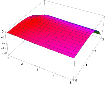
   Figure 1. Graph of $G(z,w)$ for $\beta=\beta_{c}/2<\beta_{c}$, $p=4$.

   

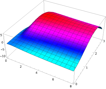
   Figure 2. Graph of $G(z,w)$ for $\beta=3\beta_{c}>\beta_{c}$, $p=4$.

7. Note the discontinuity of $\beta_{c}(p)$ at $p=\infty$. It is interesting to investigate the limiting behavior of the phase transition phenomena. In particular, it is expected that when $p=\alpha\log n$, our model would be closely related to an extremal point process behavior as $n\to\infty$. One can ask if there is another phase transition with respect to $\alpha$.

Acknowledgments. We want to thank Grigory Terlov, Kesav Krishnan, and Qiang Wu for many enlightening discussions at the beginning stage of the project. We also thank Prof. Renming Song and Prof. Christian Houdré for providing valuable references.

References

- Barthe et al. (2005) Barthe, F., O. Guédon, S. Mendelson, and A. Naor (2005). A probabilistic approach to the geometry of the -ball. Ann. Probab. 33(2), 480–513.
- Berthet et al. (2019) Berthet, Q., P. Rigollet, and P. Srivastava (2019). Exact recovery in the Ising blockmodel. Ann. Statist. 47(4), 1805–1834.
- Cerf and Gorny (2016) Cerf, R. and M. Gorny (2016). A Curie-Weiss model of self-organized criticality. Ann. Probab. 44(1), 444–478.
- Chatterjee (2007) Chatterjee, S. (2007). Stein’s method for concentration inequalities. Probab. Theory Related Fields 138(1-2), 305–321.
- Chatterjee (2017) Chatterjee, S. (2017). A note about the uniform distribution on the intersection of a simplex and a sphere. J. Topol. Anal. 9(4), 717–738.
- Chatterjee and Shao (2011) Chatterjee, S. and Q.-M. Shao (2011). Nonnormal approximation by Stein’s method of exchangeable pairs with application to the Curie-Weiss model. Ann. Appl. Probab. 21(2), 464–483.
- Chen and Sen (2023) Chen, W.-K. and A. Sen (2023). On -Gaussian-Grothendieck problem. Int. Math. Res. Not. IMRN 2023(3), 2344–2428.
- de la Peña et al. (2009) de la Peña, V. H., T. L. Lai, and Q.-M. Shao (2009). Self-normalized processes. Probability and its Applications (New York). Springer-Verlag, Berlin. Limit theory and statistical applications.
- Dembo and Zeitouni (2010) Dembo, A. and O. Zeitouni (2010). Large deviations techniques and applications, Volume 38 of Stochastic Modelling and Applied Probability. Springer-Verlag, Berlin. Corrected reprint of the second (1998) edition.
- Dominguez (2022) Dominguez, T. (2022). The -Gaussian-Grothendieck problem with vector spins. Electron. J. Probab. 27, Paper No. 70, 46.
- Dufresne (2010) Dufresne, D. (2010). distributions and the beta-gamma algebra. Electron. J. Probab. 15, no. 71, 2163–2199.
- Eisele and Ellis (1988) Eisele, T. and R. S. Ellis (1988). Multiple phase transitions in the generalized Curie-Weiss model. J. Statist. Phys. 52(1-2), 161–202.
- Ellis (2006) Ellis, R. S. (2006). Entropy, large deviations, and statistical mechanics. Classics in Mathematics. Springer-Verlag, Berlin. Reprint of the 1985 original.
- Ellis and Newman (1978) Ellis, R. S. and C. M. Newman (1978). Limit theorems for sums of dependent random variables occurring in statistical mechanics. Z. Wahrsch. Verw. Gebiete 44(2), 117–139.
- Fedele and Contucci (2011) Fedele, M. and P. Contucci (2011). Scaling limits for multi-species statistical mechanics mean-field models. J. Stat. Phys. 144(6), 1186–1205.
- Friedli and Velenik (2018) Friedli, S. and Y. Velenik (2018). Statistical mechanics of lattice systems. Cambridge University Press, Cambridge. A concrete mathematical introduction.
- Gallo and Contucci (2008) Gallo, I. and P. Contucci (2008). Bipartite mean field spin systems. Existence and solution. Math. Phys. Electron. J. 14, Paper 1, 21.
- Gorny (2014) Gorny, M. (2014). A Curie-Weiss model of self-organized criticality: the Gaussian case. Markov Process. Related Fields 20(3), 563–576.
- Gorny and Varadhan (2015) Gorny, M. and S. R. S. Varadhan (2015). Fluctuations of the self-normalized sum in the Curie-Weiss model of SOC. J. Stat. Phys. 160(3), 513–518.
- Khot and Naor (2012) Khot, S. and A. Naor (2012). Grothendieck-type inequalities in combinatorial optimization. Comm. Pure Appl. Math. 65(7), 992–1035.
- Kirsch and Toth (2022) Kirsch, W. and G. Toth (2022). Limit theorems for multi-group Curie-Weiss models via the method of moments. Math. Phys. Anal. Geom. 25(4), Paper No. 24, 43.
- Knöpfel et al. (2020) Knöpfel, H., M. Löwe, K. Schubert, and A. Sinulis (2020). Fluctuation results for general block spin Ising models. J. Stat. Phys. 178(5), 1175–1200.
- Nam (2020) Nam, K. (2020). Large deviations and localization of the microcanonical ensembles given by multiple constraints. Ann. Probab. 48(5), 2525–2564.
- Sato (2013) Sato, K.-i. (2013). Lévy processes and infinitely divisible distributions (Revised ed.), Volume 68 of Cambridge Studies in Advanced Mathematics. Cambridge University Press, Cambridge. Translated from the 1990 Japanese original.
- Schechtman and Zinn (1990) Schechtman, G. and J. Zinn (1990). On the volume of the intersection of two balls. Proc. Amer. Math. Soc. 110(1), 217–224.