Flip Dynamics for Sampling Colorings: Improving $(11/6-\varepsilon)$ Using A Simple Metric

Abstract

We present improved bounds for randomly sampling $k$-colorings of graphs with maximum degree $\Delta$; our results hold without any further assumptions on the graph. The Glauber dynamics is a simple single-site update Markov chain. Jerrum (1995) proved an optimal $O(n\log{n})$ mixing time bound for Glauber dynamics whenever $k>2\Delta$ where $\Delta$ is the maximum degree of the input graph. This bound was improved by Vigoda (1999) to $k>(11/6)\Delta$ using a “flip” dynamics which recolors (small) maximal 2-colored components in each step. Vigoda’s result was the best known for general graphs for 20 years until Chen et al. (2019) established optimal mixing of the flip dynamics for $k>(11/6-\varepsilon)\Delta$ where $\varepsilon\approx 10^{-5}$. We present the first substantial improvement over these results. We prove an optimal mixing time bound of $O(n\log{n})$ for the flip dynamics when $k\geq 1.809\Delta$. This yields, through recent spectral independence results, an optimal $O(n\log{n})$ mixing time for the Glauber dynamics for the same range of $k/\Delta$ when $\Delta=O(1)$. Our proof utilizes path coupling with a simple weighted Hamming distance for “unblocked” neighbors.

1 Introduction

A problem of great interest and considerable study at the intersection of theoretical computer science, discrete mathematics, and statistical physics is the random sampling of $k$-colorings of a given input graph $G$. Given a graph $G=(V,E)$ of maximum degree $\Delta$ and an integer $k\geq 2$, let $\Omega$ denote the collection of proper vertex $k$-colorings of $G$, that is $\Omega$ is the collection of assignments $X_{t}:V\rightarrow\{1,\dots,k\}$ where for all $(v,w)\in E$, $X_{t}(v)\neq X_{t}(w)$. Let $\pi$ denote the uniform distribution over $\Omega$. The colorings problem is a natural example of a non-binary graphical model [Mur12, KF09] and, in statistical physics, it is the zero-temperature limit of the antiferromagnetic Potts model [SS97].

We study algorithms for the approximate counting problem of estimating $\lvert\Omega\rvert$, the number of $k$-colorings, and the approximate sampling problem of generating random $k$-colorings from a nearly uniform distribution. In particular, given a graph $G=(V,E)$ and a $\delta>0$, for the sampling problem, our goal is to sample from a distribution $\mu$ which is within total variation distance $\leq\epsilon$ of the uniform distribution $\pi$ in time polynomial in $n=|V|$ and $\log(1/\varepsilon)$. In the approximate counting problem, a graph $G=(V,E)$, an $\varepsilon,$ and a $\delta>0$ are given, and the goal is to obtain a $\mathsf{FPRAS}$ to estimate $|\Omega|$, which is an algorithm to estimate $|\Omega\rvert$ within a $(1\pm\varepsilon)$ multiplicative factor with probability $\geq 1-\delta$ in time $\mathrm{poly}(n,1/\varepsilon,\log(1/\delta))$. These approximate sampling/counting problems are polynomial-time inter-reducible to each other. Relevant for our work, an $O(n\log(n/\varepsilon))$ sampling algorithm yields an $O^{*}(n^{2})$ time-approximate counting algorithm [ŠVV09, Hub15, Kol18].

The Markov chain Monte Carlo (MCMC) method is a natural algorithmic approach to approximate sampling. The Glauber dynamics (also known as the Gibbs sampler) is the simplest example of the MCMC method. The Glauber dynamics is a Markov chain on the collection of $k$-colorings and the transitions update the coloring at a randomly chosen vertex in each step as follows. From a coloring $X_{t}\in\Omega$, choose a vertex $v\in V$ and a color $c\in\{1,\dots,k\}$ uniformly at random. If no neighbor of $v$ has color $c$ in the current coloring $X_{t}$ then we recolor $v$ to color $c$ in $X_{t+1}$ and all other vertices maintain the same color $X_{t+1}(w)=X_{t}(w)$ for all $w\neq v$; and if color $c$ is not available for $v$ then we set $X_{t+1}=X_{t}$. The Glauber dynamics is ergodic whenever $k\geq\Delta+2$; hence, the unique stationary distribution is the uniform distribution $\pi$.

The mixing time $T_{\mathrm{mix}}$ is the number of steps from the worst initial state $X_{0}$ to guarantee that the total variation distance from the stationary distribution $\pi$ is $\leq 1/4$. A mixing time of $O(n\log{n})$ is referred to as an optimal mixing time as this matches the lower bound established by Hayes and Sinclair [HS07] for any graph of constant maximum degree $\Delta$.

Jerrum [Jer95] (see also Salas and Sokal [SS97]) established an optimal mixing time of $O(n\log{n})$ for the Glauber dynamics whenever $k>2\Delta$. This was a seminal result in the development of coupling techniques, including the path coupling method of Bubley and Dyer [BD97]. Vigoda [Vig99] improved Jerrum’s result to $k>(11/6)\Delta$ by proving $O(n\log{n})$ mixing time of the following flip dynamics, which implied $O(n^{2})$ mixing time of the Glauber dynamics.

The flip dynamics is a generalization of the Glauber dynamics, which recolors maximal two-colored components in each step. For a coloring $X_{t}$, vertex $v\in V$, and color $c\in\{1,\dots,k\}$, let $S_{X_{t}}(v,c)$ denote the set of vertices $w$ which have an alternating path on colors $(X_{t}(v),c)$ from $v$ to $w$; we refer to the set $S_{X_{t}}(v,c)$ as a cluster. The flip dynamics is defined by a set of parameters $(P_{i})_{i\geq 1}$ for the flip probabilities. The dynamics operates by choosing a random vertex $v$ and color $c$, and then ‘flipping’ the cluster $S_{X_{t}}(v,c)$ by interchanging the colors $X_{t}(v)$ and $c$ on the chosen cluster with probability $P_{\ell}/\ell$ where $\ell=|S_{X_{t}}(v,c)|$. In Vigoda’s original work, the parameters satisfy the basic properties: $P_{1}=1$, $P_{i}\geq P_{i+1}$ for all $i\geq 1$, and $P_{j}=0$ for $j\geq 7$, see Section 3.1 for more details. All subsequent works (including this paper) follow these broad settings but differ in the detailed setting. Note the flip dynamics is a generalization of the Glauber dynamics which corresponds to the setting: $P_{1}=1$ and $P_{j}=0$ for all $j\geq 2$.

Since Vigoda’s result, there was a myriad of improved results for various restricted classes of graphs, including optimal mixing on triangle-free graphs when $k>\alpha^{*}\Delta$ for $\Delta=O(1)$ where $\alpha^{*}\approx 1.763$ [CGŠV21, FGYZ21, CLV21] (see also [JPV22, LSS19, DFHV13] for related results), optimal mixing on large girth graphs when $k\geq\Delta+3$ [CLMM23], and further improvements for trees [MSW04], planar graphs [HVV15], and sparse random graphs [EHSV18].

The first improvement on Vigoda’s result for general graphs was 20 years later by Chen, Delcourt, Moitra, Perarnau, and Postle [CDM⁺19] who proved the mixing of $O(n\log{n})$ of the flip dynamics when $k>(11/6-\varepsilon_{0})\Delta$ where $\varepsilon_{0}\approx 10^{-5}$ is a fixed positive constant. Their result (as well as Vigoda’s result [Vig99]) was obtained for a specific setting of the flip parameters. We present the first substantial improvement over Vigoda’s result in obtaining optimal mixing of the flip dynamics when $k\geq 1.809\Delta$ for any $\Delta$.

Theorem 1.1.

For all $\Delta\geq 125$, for all $k\geq 1.809\Delta$, there exists a setting of the parameters for the flip dynamics with $P_{j}=0$ for all $j\geq 7$, so that for any graph $G$ on $n$ vertices with maximum degree $\Delta$, the flip dynamics has mixing time $O(n\log(n))$.

The flip probabilities are presented in Section 3.1. Note we use a universal setting of the flip probabilities for all $1.809\leq k<11/6$, and when $k\geq(11/6)\Delta$ then one can use the flip probabilities from [CDM⁺19, Vig99].

As in [Vig99, CDM⁺19] this implies polynomial mixing of the Glauber dynamics for the same range of $k/\Delta$. In particular, by comparison of the spectral gaps of the transition matrices, it implies $O(n^{2})$ mixing time of the Glauber dynamics where the hidden constant is polynomial in $\Delta$ and $k$ (see Section 4.6 for more details). Moreover, recent work of [BCC⁺22, Liu21] utilizing spectral independence [CLV21, ALO20], implies $O(n\log{n})$ mixing time of the Glauber dynamics when $\Delta$ is constant; the same result held for the previous work of [CDM⁺19] for the corresponding range of parameters $k$ and $\Delta$.

Corollary 1.2.

For all $\Delta\geq 125$, there exists a constant $C=C(\Delta)$ such that for any $k\geq 1.809\Delta$ and for any graph $G$ on $n$ vertices with maximum degree $\Delta$, the mixing time of the Glauber dynamics is $\leq Cn\log{n}$.

Our proof of Theorem 1.1 utilizes a novel distance metric described here at a high level.

Jerrum’s bound of $k>2\Delta$ can be proved using path coupling in which we consider a pair of configurations $X_{t},Y_{t}$ that differ at exactly one vertex, say $v^{*}$. We then analyze the expected Hamming distance of $X_{t+1},Y_{t+1}$ after one step of a coupled transition $(X_{t},Y_{t})\rightarrow(X_{t+1},Y_{t+1})$. The coupling in this setting is fairly simple as it is the identity coupling (i.e., both chains attempt the same (vertex, color) pair $(v,c)$) for the Glauber update except when the updated vertex $v$ is a neighbor $w$ of $v^{*}$; in which case we couple trying to recolor $w$ to color $X_{t}(v^{*})$ in one chain with color $Y_{t}(v^{*})$ in the other chain. Under this coupling, there is at most one coupled transition per neighbor which can increase the Hamming distance by at most one, and this yields the $k>2\Delta$ bound.

Vigoda’s result for $k>(11/6)\Delta$ uses the same path coupling framework to analyze the expected Hamming distance for a pair $X_{t},Y_{t}$ that differ at a single vertex $v^{*}$. In flip dynamics, the coupling is more complicated than in Jerrum’s analysis because of additional moves.

Recall that the transitions of the flip dynamics correspond to flipping maximal 2-colored components, where flipping refers to interchanging the $2$ colors. An alternative and equivalent view of the transitions of the flip dynamics is as follows: For $X_{t}$, consider the collection of all clusters (where a cluster is a maximal 2-colored component); note that there are at most $nk$ clusters. Choose a cluster $S$ with probability $P_{|S|}/(nk)$ and then flip $S$ to obtain $X_{t+1}$ (with the remaining probability set $X_{t+1}=X_{t}$).

We give a brief high-level overview of Vigoda’s coupling $(X_{t},Y_{t})\rightarrow(X_{t+1},Y_{t+1})$ which is the one-step coupling that for a Hamming distance one pair of colorigns minimizes the expected Hamming distance at time $t+1$ and hence is called the greedy coupling in [CDM⁺19]. Consider a pair $X_{t},Y_{t}$ that differ at a single vertex $v^{*}$, thus $X_{t}(w)=Y_{t}(w)$ for all $w\neq v^{*}$. The coupling uses the identity coupling for all clusters $S$ that are the same in chains $X_{t}$ and $Y_{t}$. This means that the cluster $S$ is flipped in both chains or in neither chain. The only nontrivial couplings are for those clusters that appear in only one chain (and not in the other chain).

What are these clusters that appear in exactly one chain? They are clusters that include a neighbor $w$ of $v^{*}$ and a color $c^{\prime}$ which is $X_{t}(v^{*})$ or $Y_{t}(v^{*})$. In other words, if we try to recolor some $w\in N(v^{*})$ to a color $c^{\prime}\in\{X_{t}(v^{*}),Y_{t}(v^{*})\}$ then this yields a different cluster in the two chains, as the cluster includes $v^{*}$ in one chain but not in the other chain. These are the clusters that use a nontrivial coupling. Moreover, this coupling depends on the current color $c=X_{t}(w)=Y_{t}(w)$ of the neighbor $w$ of $v^{*}$; we partition the clusters involving color $c$ into a set $\mathcal{D}_{t,c}$ and clusters within $\mathcal{D}_{t,c}$ are coupled with other clusters in the same set $\mathcal{D}_{t,c}$.

Vigoda demonstrated a choice of the flip probabilities and a coupling so that the expected increase in the Hamming distance is $\leq 5/6$ in an amortized cost per neighbor $w$ of $v^{*}$, which yields the bound $k>(11/6)\Delta$. Chen et al. [CDM⁺19] identified $6$ extremal configurations in Vigoda’s analysis (these are the configurations that maximize the expected increase in the Hamming distance) and presented a slightly different setting of the flip probabilities with only two extremal configurations. They considered a weighted Hamming distance where for every neighbor $w\in N(v^{*})$, if the local configuration around $w$ is different from the two extremal configurations, then the definition of the distance (between $X_{t}$ and $Y_{t}$) is decreased by $\eta/\Delta$ for a fixed constant $\eta$ where $1/2>\eta>0$. Using Vigoda’s greedy coupling with this new metric, they established that the expected distance decreases when $k>(11/6-\varepsilon_{0})\Delta$ where $\varepsilon_{0}\approx 10^{-5}$.

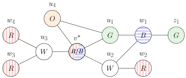
Figure 1: A small graph showing how vertices can be unblocked, singly blocked, and multiblocked. The vertex $u_{1}$ is singly blocked with respect to $v^{*}$ since it has a neighbor $w_{1}$ that is colored $B$. The vertex $u_{2}$ is multiblocked with respect to $v^{*}$ since it has a $B$ and $R$ neighbor, $w_{1}$ and $w_{2}$ respectively. Likewise, $u_{3}$ is multiblocked since it has two $R$ neighbors, $w_{3}$ and $w_{4}$. Finally, $u_{4}$ is unblocked since it has no neighbors that are $R$ or $B$.

We take a complementary approach. Whereas Chen et al. [CDM⁺19] reweight the worst configurations (or equivalently all non-worst case configurations), we instead consider a particularly “good” configuration. Namely, we consider the local configuration where the neighbor $w$ is unblocked, which means that the colors $X_{t}(v^{*})$ and $Y_{t}(v^{*})$ do not appear in $N(w)\setminus\{v^{*}\}$, see Fig. 1. Unblocked neighborhoods are the best local configurations for the greedy coupling (with respect to the Hamming distance). For unblocked neighbors $w$, the potentially problematic recolorings of $w\in N(v^{*})$ with colors $X_{t}(v^{*})$ or $Y_{t}(v^{*})$ can be coupled with flips of clusters of size 2 (containing $v^{*}$ and $w$). Consequently, the expected increase in the Hamming distance for $w$ is $1-P_{2}$, significantly less than $5/6$ for any setting of the flip probabilities considered.

We choose the flip probabilities to optimize for this new metric, which results in a setting for the flip probabilities that are suboptimal (with respect to Hamming distance) for the extremal configurations considered by Chen et al. [CDM⁺19]. However, for our choice of distance metric, these extremal configurations improve as they have a reasonable probability of moving to the unblocked configurations, yielding a decrease in the distance.

An essential aspect of our proof is that if a neighbor $w$ is unblocked, then it may have a considerable probability of becoming blocked (which increases the distance with respect to our new metric); however, in this case, if $w$ itself becomes a disagreement, then its neighbors will be unblocked (and hence this new disagreement at $w$ has a smaller weight in our new metric). This is the crucial trade-off in our argument: For an unblocked neighbor $w$, either $w$ is unlikely to become blocked, or if it becomes a disagreement, it has many unblocked neighbors. Our overall proof is of a similar technical level of difficulty as in [CDM⁺19] but yields a substantially improved bound of $k\geq 1.809\Delta$.

We present some basic definitions, including a more formal definition of the flip dynamics, and the path coupling lemma in Section 2. In Section 3 we define our new metric. We then present Vigoda’s greedy coupling, analyze our new metric, and prove Theorem 1.1 in Section 4.

2 Preliminaries

2.1 Neighboring Colorings

For positive integer $k$, let $[k]=\{1,\dots,k\}$. Let $\Omega=[k]^{V}$ be the collection of all $k$-labelings of $G$, and let $\Omega^{*}\subset\Omega$ denote the collection of proper $k$-colorings, i.e., for $\sigma\in\Omega^{*}$, for all $(v,w)\in E$, $\sigma(v)\neq\sigma(w)$.

For a pair $X_{t},Y_{t}\in\Omega$, let $H(X_{t},Y_{t})=|\{v\in V:X_{t}(v)\neq Y_{t}(v)\}|$ denote the Hamming distance between $X_{t}$ and $Y_{t}$. Let $\Lambda\subset\Omega^{2}$ denote the pairs $(X_{t},Y_{t})\in\Omega^{2}$ where $H(X_{t},Y_{t})=1$. Moreover, for $v\in V$, let $\Lambda_{v}\subset\Lambda$ where $X_{t}(v)\neq Y_{t}(v)$; thus, $\Lambda_{v}$ is the set of pairs of labelings that only differ at vertex $v$. Note, $\Lambda=\bigcup_{v\in V}\Lambda_{v}$. We will refer to pairs $(X_{t},Y_{t})\in\Lambda$ as neighboring colorings. For simplicity, we use the term coloring throughout since the distinction between colorings and labelings is clear from the notation $\Omega$ vs. $\Omega^{*}$.

2.2 Clusters, Flip Dynamics, and Mixing Time

For a coloring $X_{t}\in\Omega$, vertex $v\in V$, and color $c\in[k]$, let $S_{X_{t}}(v,c)$ denote the set of vertices reachable from $v$ by a $(X_{t}(v),c)$ alternating path in $X_{t}$. Note that $X_{t}$ may not be a proper coloring, but we still require that the colors alternate along the path. For all $v\in V$, let $S_{X_{t}}(v,X_{t}(v))=S_{Y_{t}}(v,Y_{t}(v))=\emptyset$. For a coloring $X_{t}\in\Omega$ and a cluster $S=S_{X_{t}}(v,c)$, we refer to “flipping” cluster $S$ with the operation of interchanging colors $X_{t}(v)$ and $c$ on the set $S$; let $X_{t+1}$ denote the resulting coloring. If $X_{t}$ is a proper coloring, then $X_{t+1}$ is a proper coloring. Moreover, if $X_{t},X_{t+1}$ are proper colorings then by flipping $S^{\prime}=S_{X_{t+1}}(v,X_{t}(v))$ in $X_{t+1}$ we obtain $X_{t}$, and hence the operation is symmetric on $\Omega^{*}$.

We can now define the flip dynamics. Consider probabilities $(P_{i})_{i\geq 1}$. For $X_{t}\in\Omega$ the transitions $X_{t}\rightarrow X_{t+1}$ of the flip dynamics are defined as follows:

• Choose $v\in V$ and $c\in[k]$ uniformly at random.

• Let $S=S_{X_{t}}(v,c)$ and let $\ell=|S|$ denote the size of the cluster defined by vertex $v$ and color $c$.

• With probability $P_{\ell}/\ell$, let $X_{t+1}$ denote the coloring obtained by interchanging colors $X_{t}(v)$ and $c$ in $S$ (and for $w\notin S_{X_{t}}$ set $X_{t+1}(w)=X_{t}(w)$).

• With probability $1-P_{\ell}/\ell$, let $X_{t+1}=X_{t}$.

When $P_{1}=1$ and $P_{i}=0$ for all $i>1$ then the flip dynamics attempts to update a random vertex with a random color in each step and corresponds to the Glauber dynamics (see Jerrum [Jer95]). Moreover, when $P_{1}>0$ and $k\geq\Delta+2$, then the unique stationary distribution of the flip dynamics is the uniform distribution $\pi$ over $\Omega^{*}$, which is the set of proper $k$-colorings; note, the states in $\Omega\setminus\Omega^{*}$ are transient.

Our interest is the mixing time $T_{\mathrm{mix}}$, which measures the speed of convergence to the unique stationary distribution $\pi$ from the worst initial state $X_{0}\in\Omega$. For a pair of distributions $\mu,\pi$ on $\Omega$, the total variation distance is defined as $d_{\mathsf{TV}}(\mu,\pi)=\frac{1}{2}\sum_{X_{t}\in\Omega}|\mu(X_{t})-\pi(X_{t})|$. For $\varepsilon>0$, define the mixing time as:

$$T_{\mathrm{mix}}(\varepsilon)=\max_{X_{0}\in\Omega}\min\{t:d_{\mathsf{TV}}(P^{t}(X_{t},\cdot),\pi)\leq\varepsilon\},$$

where $\pi$ is the stationary distribution. We will often refer to $T_{\mathrm{mix}}=T_{\mathrm{mix}}(1/4)$ as the mixing time since $T_{\mathrm{mix}}(\varepsilon)\leq T_{\mathrm{mix}}\times\lceil\log_{2}(1/\varepsilon)\rceil$ for any $\varepsilon>0$.

2.3 Path Coupling

We will utilize the coupling method to upper-bound the mixing time. For a pair of states $X_{t},Y_{t}\in\Omega$, a coupling for the flip dynamics is a joint evolution $(X_{t},Y_{t})\rightarrow(X_{t+1},Y_{t+1})$ such that when the individual transitions $(X_{t}\rightarrow X_{t+1})$ and $(Y_{t}\rightarrow Y_{t+1})$ are viewed in isolation of each other then they are identical to the flip dynamics, see [Jer03] for a more detailed introduction.

We will bound the mixing time using the path coupling framework of Bubley and Dyer [BD97].

Theorem 2.1.

[BD97, DG99] Consider a Markov chain with transition matrix $P$, state space $\Omega$, and unique stationary distribution $\pi$. Let $\Lambda\subset\Omega^{2}$ denote a subset of pairs of states such that the graph $(\Omega,\Lambda)$ is connected. Consider weights $w(X_{t},Y_{t})$ defined for all pairs $(X_{t},Y_{t})\in\Lambda$. Assume there exists a constant $1/2\leq C\leq 1$ where $w(X_{t},Y_{t})\in[C,1]$ for all $(X_{t},Y_{t})\in\Lambda$. For arbitrary pairs $(X_{t+1},Y_{t+1})\in\Omega^{2}$, define $w(X_{t+1},Y_{t+1})$ by the length of the shortest path in the graph $(\Omega,\Lambda)$ where edges $(X_{t},Y_{t})\in\Lambda$ have weight $w(X_{t},Y_{t})$.

If there exists a $\delta>0$ and for all $(X_{t},Y_{t})\in\Lambda$ there exists a coupling $(X_{t},Y_{t})\rightarrow(X_{t+1},Y_{t+1})$ where:

$${\mathbf{E}\left[{w(X_{t+1},Y_{t+1})}\right]}\leq(1-\delta)w(X_{t},Y_{t}),$$

then the mixing time is bounded as $T_{\mathrm{mix}}(\varepsilon)\leq O\left({\log(n/\varepsilon)}/{\delta}\right)$.

3 New Metric Definition

This section introduces our new metric, the heart of the proof of Theorem 1.1. First, we describe our flip probabilities and identify some of their key properties. Then, we introduce some new notation. Finally, we define the new metric.

3.1 Cluster and Flip Dynamics

To prove Theorem 1.1, we use the following setting of flip probabilities, which we will refer to as Eq. 1:

$$P_{1}:=1,P_{2}:=0.324,P_{3}:=0.154,P_{4}:=0.088,P_{5}:=0.044,P_{6}:=0.011,\mbox{ and }P_{i}:=0\mbox{ for }i\geq 7.$$ (1)

We also include the following variable which we will use when defining our new metric:

$$\eta:=0.0469.$$ (2)

We will assume the following properties, which we will refer to as Eq. 2:

$$P_{1} =1,\ \ P_{2}\leq 1/3,\mbox{ and }P_{7}=0$$ (FP0)

$$P_{j} \leq(2/3)P_{j-1}\mbox{ for all }j\geq 3,$$ (FP1)

$$(1-P_{2}) \geq(P_{2}-P_{3})\geq 2(P_{3}-P_{4})$$ (FP2)

$$2(P_{3}-P_{4}) \geq(j-1)(P_{j}-P_{j+1})\mbox{ for }j\geq 4$$ (FP3)

$$(P_{4}-P_{5}) \geq(P_{5}-P_{6})\geq(P_{6}-P_{7})$$ (FP4)

$$2P_{2} \leq 1-4P_{4}$$ (FP5)

$$2P_{3} \leq 4P_{4}-P_{5}$$ (FP6)

$$\eta \leq(6/19)P_{2}$$ (FP7)

Note that these properties hold for Eq. 1 and the settings originally considered by Vigoda. As we will see later in our analysis, this assumption allows us to quickly identify those initial configurations with the worst expected change for our new metric (introduced in the following sections). The relevant lemma statements include any further assumptions on the flip probabilities.

Our setting for the flip probabilities also differs from those in previous works [Vig99, CDM⁺19]. One of the key differences is that the previous work sets $P_{3}\approx 1/6$. In particular, the setting $P_{3}=1/6$ was critical in [Vig99] and any setting of $P_{3}\neq 1/6$ yields a worse bound of $k>C\Delta$ for a constant $C>11/6$ using Vigoda’s analysis. In [CDM⁺19] they also fix $P_{3}=1/6$ for their analysis with a modified metric; the argument using a variable length coupling sets slightly above $1/6$, namely $P_{3}=0.166762>1/6$. In contrast, our setting of $P_{3}<1/6$ is somewhat counterintuitive at first glance as it increases the expected change in Hamming distance for the extremal configurations in Vigoda’s analysis, but the introduction of our new metric offsets this effect.

3.2 Our New Metric

Before we introduce our new metric, we need several new definitions. For an integer $s\geq 0$, consider a pair of colorings $X_{s},Y_{s}\in\Omega$; note this pair $X_{s},Y_{s}$ may differ at an arbitrary number of vertices.

For a vertex $z\in V$ such that $X_{s}(z)\neq Y_{s}(z)$, we partition the neighbors of $z$ based on how many occurrences of the colors $X_{s}(z),Y_{s}(z)$ occur in their neighborhood (besides at $z$). For a vertex $y\in N(z)$, let

$$B^{z}_{s}(y):=\{w\in N(y)\setminus\{z\}:X_{s}(w)=X_{s}(z)\mbox{ or }Y_{s}(w)=Y_{s}(z)\}$$

as the blocking neighbors of $y$ with respect to $z$ in $X_{s}$ and $Y_{s}$.

We say that a neighbor $y\in N(z)$ is unblocked with respect to $z$ if it has no blocking neighbors (i.e. $\lvert B^{z}_{s}(y)\rvert=0$), singly blocked with respect to $z$ if there is exactly one blocking neighbor (i.e. $\lvert B^{z}_{s}(y)\rvert=1$), and multiblocked otherwise (i.e. $\lvert B^{z}_{s}(y)\rvert\geq 2$).

For integer $i\geq 0$, if $X_{s}(z)\neq Y_{s}(z)$ then let

$$F^{i}_{s}(z):=\{y\in N(z):\lvert B^{z}_{s}(y)\rvert=i\}\mbox{ and }F^{\geq i}_{s}(z):=\bigcup_{j\geq i}F^{i}_{s}(z).$$

be the neighbors of $z$ with exactly $i$ (or at least $i$) blocking neighbors. Moreover, if $X_{s}(z)=Y_{s}(z)$ then let $F^{i}_{s}(z)=\emptyset$. Let

$$d^{i}_{s}(z):=\lvert F^{i}_{s}(z)\rvert\mbox{ and }d^{\geq i}_{s}(z):=\sum_{j\geq i}d^{j}_{s}(z).$$

be the number of neighbors of $z$ with exactly $i$ (or at least $i$) blocking neighbors. Notice that $F^{0}_{s}{(z)}$ is the set of unblocked neighbors of $z$ in $(X_{s},Y_{s})$, $F^{1}_{s}(z)$ is the set of singly blocked neighbors of $z$, and $F^{\geq 2}_{s}(z)$ is the set of multiblocked neighbors of $z$.

We can now formally define our new metric. Recall the definition of the constant $\eta$ from Eq. 2. For a pair $(X_{t},Y_{t})\in\Lambda_{v^{*}}$, we define the distance between these neighboring colorings as follows:

$$\widetilde{H}(X_{t},Y_{t}):=1-\frac{\eta}{\Delta}d^{0}_{t}(v^{*}).$$ (3)

Extend $\widetilde{H}$ to define a metric $\widetilde{H}$ over all pairs in $\Omega^{2}$ by considering the path metric defined by the shortest path distance in the graph $(\Omega,\Lambda)$ where neighboring colorings have weight defined by Eq. 3.

The following lemma upper bounds $\widetilde{H}$ by the Hamming metric $H$ and the number of unblocked neighbors. The bound is tight if the two states differ at exactly one vertex, $v$. Recall that if $X_{t}(u)=Y_{t}(u)$ then $F^{0}_{t}{(u)}=\emptyset$ and hence $d^{0}_{t}(u)=0$. This lemma has nothing to do with the coupling; it means that the path metric $\widetilde{H}$, which we implicitly defined for pairs $(X_{t},Y_{t})$ that differ at more than one vertex, can be bounded naturally by the Hamming distance and the number of unblocked neighbors of disagreements in $X_{t},Y_{t}$.

Consider an arbitrary pair $X_{t},Y_{t}\in\Omega$. We first define for a vertex $z\in V$,

$$H_{z}(X_{t},Y_{t}):=\begin{cases}1&\mbox{if }X_{t}(z)\neq Y_{t}(z)\\ 0&\mbox{otherwise}\end{cases}$$ (4)

and

$$\widetilde{H}_{z}(X_{t},Y_{t}):=\begin{cases}1-\frac{\eta}{\Delta}d^{0}_{t}(z)&\mbox{if }X_{t}(z)\neq Y_{t}(z)\\ 0&\mbox{otherwise.}\end{cases}$$ (5)

We can then upper bound the distance $\widetilde{H}{}$ for an arbitrary pair of colorings by the sum over disagreeing vertices.

Lemma 3.1.

For any $X_{t},Y_{t}\in\Omega$,

$$\widetilde{H}(X_{t},Y_{t})\leq\sum_{z\in V}\widetilde{H}_{z}(X_{t},Y_{t}).$$

Proof.

Let $U=\{u\in V\;:\;{Y_{t}}(u)\not={X_{t}}(u)\}$ be the set of vertices that ${X_{t}}$ and ${Y_{t}}$ disagree on and let $U=\{u_{1},\ldots,u_{\lvert U\rvert}\}$ be an arbitrary ordering of $U$. Let $\rho_{0}={X_{t}}$ and $\rho_{\lvert U\rvert}={Y_{t}}$ and for $1\leq i\leq\lvert U\rvert-1$, let $\rho_{i}(u_{j})=\rho_{i-1}(u_{j})$ for $j\not=i$ and $\rho_{i}(u_{i})={Y_{t}}(u_{i})$. It follows that

$$\widetilde{H}({X_{t}},{Y_{t}})\leq\sum_{i}\widetilde{H}(\rho_{i-1},\rho_{i})$$ (6)

since $\widetilde{H}({X_{t}},{Y_{t}})$ is defined to be the length of the shortest path between ${X_{t}}$ and ${Y_{t}}$ and the path $\rho_{0},\ldots,\rho_{\lvert U\rvert}$ is a particular path. We will prove that for all $u_{i}\in U$,

$$d^{0}(u_{i},{\rho_{i-1}},{\rho_{i}})\geq d^{0}({u_{i}},{{X_{t}}},{{Y_{t}}}).$$ (7)

Assuming Eq. 7 and making use of Eq. 6 we can conclude the lemma as follows:

$$\widetilde{H}({X_{t}},{Y_{t}}) \leq\sum_{i}\widetilde{H}(\rho_{i-1},\rho_{i})$$ (by Eq. 6)

$$=\frac{\eta}{\Delta}\sum_{u_{i}\in U}\left(1-d^{0}(u_{i},{\rho_{i-1}},{\rho_{i}})\right)$$ (by Eq. 3)

$$=H({X_{t}},{Y_{t}})-\frac{\eta}{\Delta}\sum_{u_{i}\in U}d^{0}(u_{i},{\rho_{i-1}},{\rho_{i}}) \lvert U\rvert=H(X_{t},Y_{t})$$ ()

$$\leq H({X_{t}},{Y_{t}})-\frac{\eta}{\Delta}\sum_{u_{i}\in U}d^{0}(u_{i},{X_{t}},{Y_{t}}).$$ (by Eq. 7)

It remains to prove Eq. 6, for which it suffices to show that, for all $u_{i}\in U$,

$$F^{0}(u_{i},\rho_{i-1},\rho_{i})\supseteq F^{0}(u_{i},{X_{t+1}},{Y_{t+1}}).$$

Fix $i$ and suppose $w\in F^{0}(u_{i},{X_{t}},{Y_{t}})$. We will show that $w\in F^{0}(u_{i},\rho_{i-1},\rho_{i})$. Since $w\in F^{0}(u_{i},{X_{t}},{Y_{t}})$, for all $z\in N(w)\setminus\{u_{i}\}$, $\{{X_{t}}(z),{Y_{t}}(z)\}\cap\{{X_{t}}(u_{i}),{Y_{t}}(u_{i})\}=\emptyset$. By the definition of $\rho_{i-1}$ and $\rho_{i}$, $\rho_{i}(z)=\rho_{i-1}(z)={X_{t}}(z)={Y_{t}}(z)$, $\rho_{i-1}(u_{i})={X_{t}}(u_{i})$, and $\rho_{i}(u_{i})={Y_{t}}(u_{i})$. Thus, for all $z\in N(w)\setminus\{u_{i}\}$, $\{\rho_{i-1}(z),\rho_{i}(z)\}\cap\{\rho_{i-1}(u_{i}),\rho_{i}(u_{i})\}=\emptyset$ and $w\in F^{0}(u_{i},\rho_{i-1},\rho_{i})$. ∎

4 Coupling Analysis

We start our analysis by giving a brief description of the greedy coupling.

To define the greedy coupling for the flip dynamics, let us first observe an alternative formulation of the dynamics. For a state $X_{t}\in\Omega$, every cluster $S$ in $X_{t}$ has an associated flip probability $P_{|S|}$. To simulate the flip dynamics we choose a cluster $S$ with probability $P_{|S|}/(nk)$ and then flip it to obtain the new state $X_{t+1}$, and with the remaining probability, we stay in the same state $X_{t+1}=X_{t}$.

If the same cluster occurs in both chains, the greedy coupling will flip it in both chains or not in either chain; this is referred to as the identity coupling. The only non-identity coupling is for clusters that potentially differ in the two chains. These potential disagreeing clusters involve $v^{*}$ or neighbors of $v^{*}$ and can be partitioned according to the current colors of the neighbors of $v^{*}$.

We now partition the neighbors of a vertex $z\in V$ on a per color basis. For any coloring $X_{s}\in\Omega$, a color $c$, and vertex $z\in V$, let

$$N_{c}(z,X_{s}):=\{w\in N(z)\;:\;X_{s}(z)=c\}$$

be the neighbors of $z$ that are color $c$ in $X_{s}$. We extend this notation for an arbitrary pair $X_{s},Y_{s}\in\Omega$ by letting

$$N_{s,c}(z):=N_{c}(z,X_{s})\cup N_{c}(z,Y_{s}).$$

Note that if $(X_{t},Y_{t})\in\Lambda_{v^{*}}$ then $N_{t,c}(v^{*})=N_{c}(v^{*},X_{t})=N_{c}(v^{*},Y_{t})$. Let

$$d_{t,c}(v^{*}):=\lvert N_{t,c}(v^{*})\rvert$$

be the number of neighbors of $v^{*}$ that are colored $c$ in $X_{t}$ or $Y_{t}$.

Now we will give a brief overview of the greedy coupling. Fix a pair $(X_{t},Y_{t})\in\Lambda_{v^{*}}$. The clusters involving color $c$ that we need to couple (using the greedy coupling) are the following:

$$\mathcal{D}_{t,c}:=\left\{S_{X_{t}}(v^{*},c)\right\}\cup\left\{S_{Y_{t}}(v^{*},c)\right\}\cup\bigcup_{u\in N_{t,c}(v^{*})}\{S_{X_{t}}(u,Y_{t}(v^{*})),S_{Y_{t}}(u,X_{t}(v^{*}))\}.$$ (8)

Let us digest this collection of clusters $\mathcal{D}_{t,c}$. Consider the case when $d_{t,c}(v^{*})=0$, then $\mathcal{D}_{t,c}$ consists of two clusters $S_{X_{t}}(v^{*},c)$ and $S_{Y_{t}}(v^{*},c)$, and both of these clusters are the same: $S_{X_{t}}(v^{*},c)=S_{Y_{t}}(v^{*},c)=\{v^{*}\}$ since color $c$ does not appear in the neighborhood of $v^{*}$. These clusters are coupled with the identity coupling, which means that we flip the cluster in both chains or neither chain. Note that if we flip these clusters $S_{X_{t}}(v^{*},c)=S_{Y_{t}}(v^{*},c)$ when $d_{t,c}(v^{*})=0$ then the resulting colorings are the same $X_{t+1}=Y_{t+1}$ (as $X_{t+1}(v^{*})=Y_{t+1}(v^{*})=c$); these are the “good” moves which decrease the Hamming distance by one.

The nontrivial case is when $d_{t,c}(v^{*})\geq 1$. The clusters of $\mathcal{D}_{t,c}$ which occur in $X_{t}$, are the $S_{X_{t}}(w,Y_{t}(v^{*}))$ cluster for every $w\in N_{t,c}(v^{*})$ and the $S_{X_{t}}(v^{*},c)$ cluster; and in $Y_{t}$ we have the $S_{X_{t}}(w,X_{t}(v^{*})$ for $w\in N_{t,c}(v^{*})$ and the $S_{Y_{t}}(v^{*},c)$ cluster. Notice that these two $(v^{*},c)$ clusters are large clusters that consist of the union of the other small clusters plus $v^{*}$, namely,

$$S_{X_{t}}(v^{*},c)=\{v^{*}\}\cup\bigcup_{w\in N_{t,c}(v^{*})}S_{Y_{t}}(w,X_{t}(v^{*}))\ \ \mbox{ and }\ \ S_{Y_{t}}(v^{*},c)=\{v^{*}\}\cup\bigcup_{w\in N_{t,c}(v^{*})}S_{X_{t}}(w,Y_{t}(v^{*})).$$

The only non-identity coupling involves clusters in $\mathcal{D}_{t,c}$ for some $c$ where $d_{t,c}(v^{*})\geq 1$. The clusters in $\mathcal{D}_{t,c}$ are coupled with each other (or with nothing corresponding to a self-loop in the other chain); the greedy coupling in these cases is detailed in Section 5.1.

We define the set of vertices besides $v^{*}$ that are contained in a cluster of $\mathcal{D}_{t,c}$ as

$$\mathcal{L}_{t,c}:=\{u\in V\setminus\{v^{*}\}:\mbox{ there exists }S\in\mathcal{D}_{c}(X_{t},Y_{t})\mbox{ such that }u\in S\}.$$

That is, $\mathcal{L}_{t,c}$ is every vertex besides $v^{*}$ that can be reached from $v^{*}$ with a $(c,X_{t}(v^{*}))$ or $(c,Y_{t}(v^{*}))$ alternating path. These are precisely the vertices where new disagreements can form after a single step of the greedy coupling. Observe that $N_{t,c}(v^{*})\subseteq\mathcal{L}_{t,c}$.

4.1 Relating $\widetilde{H}$ to $H$

Fix a pair $(X_{t},Y_{t})\in\Lambda_{v^{*}}$. Let

$$W_{t}:={\mathbf{E}\left[{H(X_{t+1},Y_{t+1})-H(X_{t},Y_{t})}\right]}$$

and

$$\widetilde{W}_{t}:={\mathbf{E}\left[{\widetilde{H}(X_{t+1},Y_{t+1})-\widetilde{H}(X_{t},Y_{t})}\right]}$$ (9)

denote the expected change over one step of the greedy coupling, $(X_{t},Y_{t})\rightarrow(X_{t+1},Y_{t+1})$, for $H$ and $\widetilde{H}$ respectively. The following subsections aim to bound $\widetilde{W}_{t}$ by decomposing it with respect to each color.

4.2 Analysis by Color

We want to decompose the expected change in the Hamming distance $W_{t}$ and our metric $\widetilde{W}_{t}$ with respect to each color $c$.

Recall $H_{z}$ is the Hamming distance at a vertex $z$, see Eq. 4. Fix colorings $X_{s},Y_{s}\in\Omega$. We define the Hamming distance with respect to an arbitrary subset $R\subseteq V$ as

$$H_{R}(X_{s},Y_{s}):=\sum_{z\in R}H_{z}(X_{s},Y_{s}).$$

Similarly, we define the new metric distance with respect to an arbitrary subset $R\subseteq V$ and vertex $z\not\in R$ as

$$\widetilde{H}_{z,R}(X_{s},Y_{s}):=H_{R}(X_{s},Y_{s})-\frac{\eta}{\Delta}\left(\lvert F^{0}_{s}{(z)}\cap R\rvert+\sum_{y\in R}\rvert F^{0}_{s}{(y)}\lvert\right).$$ (10)

We will give some intuition for the definition of $\widetilde{H}_{z,R}(X_{s},Y_{s})$ in Eq. 10 after the statement of Lemma 4.1 below.

We can now define for all pairs $(X_{t},Y_{t})\in\Lambda_{v^{*}}$ and for all $c$ such that $d_{t,c}(v^{*})\geq 1$,

$$W^{c}_{t}:={\mathbf{E}\left[{H_{\mathcal{L}_{t,c}}(X_{t+1},Y_{t+1})-H_{\mathcal{L}_{t,c}}(X_{t},Y_{t})}\right]}$$

and

$$\widetilde{W}^{c}_{t}:={\mathbf{E}\left[{\widetilde{H}_{v^{*},\mathcal{L}_{t,c}}(X_{t+1},Y_{t+1})-\widetilde{H}_{v^{*},\mathcal{L}_{t,c}}(X_{t},Y_{t})}\right]}$$ (11)

as the expected change concerning $\mathcal{L}_{t,c}$, which are the vertices related to color $c$. Notice that both terms for $W^{c}_{t}$ (and also $\widetilde{W}^{c}_{t}$) the set $R=\mathcal{L}_{t,c}$ which is defined for time $t$.

We will show that if we bound these new functions $W^{c}_{t}$ and $\widetilde{W}^{c}_{t}$ for every color $c$ such that $d_{t,c}(v^{*})\geq 1$, then we obtain an upper bound on the total change as follows:

Lemma 4.1.

For $(X_{t},Y_{t})\in\Lambda_{v^{*}}$,

$$\widetilde{W}_{t}\leq{\mathbf{E}\left[{H_{v^{*}}(X_{t+1},Y_{t+1})-H_{v^{*}}(X_{t},Y_{t})}\right]}+\sum_{c\in[k]:\atop d_{t,c}(v^{*})\geq 1}\widetilde{W}^{c}_{t}.$$

In Lemma 4.1, the ${\mathbf{E}\left[{H_{v^{*}}(X_{t+1},Y_{t+1})-H_{v^{*}}(X_{t},Y_{t})}\right]}$ term is capturing the change in Hamming distance at $v^{*}$. For the change in the new metric at $v^{*}$ we also need to capture the change in the number of unblocked neighbors of $v^{*}$; these terms are considered based on the colors of the neighbors of $v^{*}$ and are captured in the second term in Eq. 10, namely $\lvert F^{0}_{t}{(v^{*})}\cap\mathcal{L}_{t,c}\rvert$. Finally, the change in the new metric for all other vertices (besides $v^{*}$) are also considered on a per color basis and captured by the last summation in Eq. 10.

Proof of Lemma 4.1.

Since $(X_{t},Y_{t})\in\Lambda_{v^{*}}$ we have that:

$$\widetilde{H}(X_{t},Y_{t}) =\widetilde{H}_{v^{*}}(X_{t},Y_{t})$$

$$=H_{v^{*}}(X_{t},Y_{t})+\sum_{c\in[k]:\atop d_{t,c}(v^{*})\geq 1}\widetilde{H}_{v^{*},\mathcal{L}_{t,c}}(X_{t},Y_{t}).$$ (12)

For a vertex $u\in V$, observe that if $u\neq v^{*}$ then $X_{t}(u)=Y_{t}(u)$, and if for all colors $c\in[k]$ we have $u\not\in\mathcal{L}_{t,c}$ then every cluster that contains $u$ is in both $X_{t}$ and $Y_{t}$ and hence $X_{t+1}(u)=Y_{t+1}(u)$, since the greedy coupling either flips a cluster containing $u$ in both chains or neither (see Section 5.1). Therefore, $H_{u}(X_{t+1},Y_{t+1})=0$ and $\widetilde{H}_{u}(X_{t+1},Y_{t+1})=0$ by definition. In summary, we have the following:

$$\sum_{u\notin\bigcup_{c}\mathcal{L}_{t,c}:\atop u\neq v^{*}}\widetilde{H}_{u}(X_{t+1},Y_{t+1})=0.$$ (13)

This yields the following decomposition of the new metric at time $t+1$:

$$\widetilde{H}(X_{t+1},Y_{t+1}) \leq\sum_{u\in V}\widetilde{H}_{u}(X_{t+1},Y_{t+1})$$ (by Lemma 3.1)

$$\leq\widetilde{H}_{v^{*}}(X_{t+1},Y_{t+1})+\sum_{c\in[k]:\atop d_{t,c}(v^{*})\geq 1}\sum_{u\in\mathcal{L}_{t,c}}\widetilde{H}_{u}(X_{t+1},Y_{t+1})$$ (by Eq. 13)

$$=H_{v^{*}}(X_{t+1},Y_{t+1})+\sum_{c\in[k]:\atop d_{t,c}(v^{*})\geq 1}\widetilde{H}_{v^{*},\mathcal{L}_{t,c}}(X_{t+1},Y_{t+1})$$ (by Definition 10) (14)

where the second inequality is in fact an equality for a graph with sufficiently high girth.

We can now use Eqs. 12 and 14 to finish the proof:

$$\widetilde{W}_{t} ={\mathbf{E}\left[{\widetilde{H}(X_{t+1},Y_{t+1})-\widetilde{H}(X_{t},Y_{t})}\right]}\hskip 180.67499pt\mbox{(by Definition \ref{def:wt})}$$

$$\leq{\mathbf{E}\left[{H_{v^{*}}(X_{t+1},Y_{t+1})-H_{v^{*}}(X_{t},Y_{t})}\right]}+\sum_{c\in[k]:\atop d_{t,c}(v^{*})\geq 1}{\mathbf{E}\left[{\widetilde{H}_{v^{*},t,c}(X_{t+1},Y_{t+1})-\widetilde{H}_{v^{*},t,c}(X_{t},Y_{t})}\right]}$$

$$={\mathbf{E}\left[{H_{v^{*}}(X_{t+1},Y_{t+1})-H_{v^{*}}(X_{t},Y_{t})}\right]}+\sum_{c\in[k]:\atop d_{t,c}(v^{*})\geq 1}\widetilde{{W}}^{c}_{t}\hskip 97.56493pt\mbox{(by Definition \ref{def:wct}),}$$

where the second line follows from Eqs. 12 and 14. This completes the proof of the lemma. ∎

4.3 Vertices Changing Between Blocked and Unblocked

Fix $(X_{t},Y_{t})\in\Lambda_{v^{*}}$. Our goal now is to bound $\widetilde{W}^{c}_{t}$ for all $c$. Recall $d_{t,c}(v^{*})=\lvert N_{t,c}(v^{*})\rvert$. Now let

$$d^{i}_{t,c}(v^{*}):=\lvert N_{t,c}(v^{*})\cap F^{i}_{t}(v^{*})\rvert$$

be the number of neighbors of $v^{*}$ that are colored $c$ in $X_{t}$ or $Y_{t}$ and have exactly $i$ blocking neighbors with respect to $v^{*}$. For $i\geq 1$, let

$$\Delta_{i}=\Delta_{i,t}(v^{*}):=\lvert\{u\in N(v^{*}):d_{X_{t}(u)}=d_{Y_{t}(u)}=i\}\rvert$$

denote the number of neighbors whose color appears exactly $i$ times in the neighborhood of $v^{*}$. Finally, let $\mathcal{A}_{t}(v^{*})=\{c\in[k]:d_{t,c}(v^{*})=0\}$ be the set of “available” colors for $v^{*}$ in $X_{t}$ and $Y_{t}$.

The following function will serve as an upper bound on $\widetilde{W}^{c}_{t}$ and is a function of $W^{c}_{t}$, $d^{0}_{t,c}(v^{*})$, and $d^{1}_{t,c}(v^{*})$. The quantities $\alpha$ and $\beta$ will appear in later lemmas.

Definition 4.2.

Let $\alpha:=(k-\Delta-2)$ and $\beta:=k-P_{2}\left(\Delta_{1}+\Delta_{2}\right)+(1+P_{2})\Delta$. Then for $(X_{t},Y_{t})\in\Lambda_{v^{*}}$, let

$$nk\widetilde{Z}^{c}_{t} :=nkW^{c}_{t}+d^{0}_{t,c}(v^{*})\frac{\eta\beta}{\Delta}-d^{1}_{t,c}(v^{*})\frac{\eta\alpha}{\Delta}.$$

The following lemma shows that it suffices to bound $\widetilde{Z}^{c}_{t}$ instead of $\widetilde{W}^{c}_{t}$ directly. We will later be able to show that $\widetilde{Z}^{c}_{t}$ is maximized in just a few cases, which we can analyze individually.

Lemma 4.3.

For $(X_{t},Y_{t})\in\Lambda_{v^{*}}$ and $c\in[k]$,

$$\widetilde{W}^{c}_{t} \leq\widetilde{Z}^{c}_{t}.$$

To prove Lemma 4.3, we use the following two lemmas that bound the expected number of vertices colored $c$ in $X_{t}$ and $Y_{t}$ that become blocked or unblocked after a single step of the greedy coupling.

We first give a lower bound on the number of newly unblocked neighbors of $v^{*}$. In particular, for a color $c$, we lower bound the probability that for a neighbor $w$ which is colored $c$ in $X_{t}$ and $Y_{t}$, that $w$ becomes unblocked after a single step of the greedy coupling.

Lemma 4.4.

Let $\alpha:=(k-\Delta-2)$. Then for $(X_{t},Y_{t})\in\Lambda_{v^{*}}$ and color $c$ such that $d_{t,c}(v^{*})\geq 1$,

$${\mathbf{E}\left[{\lvert(F^{0}_{t+1}{(v^{*})}\setminus F^{0}_{t}{(v^{*})})\cap N_{t,c}(v^{*})\rvert}\right]}\geq d^{1}_{t,c}(v^{*})\frac{\alpha}{nk}.$$

Proof.

Let $u\in F^{1}_{t}(v^{*})\cap N_{t,c}(v^{*})$. Since $u$ is a singly blocked neighbor of $v^{*}$ there must exist a unique neighbor $w\in N(u)\setminus(N(v^{*})\cup\{v^{*}\})$ where $X_{t}(w)\in\{X_{t}(v^{*}),Y_{t}(v^{*})\}$. There are at least $\lvert\mathcal{A}_{t}(v^{*})\setminus\{X_{t}(v^{*}),Y_{t}(v^{*})\}\rvert\geq k-\Delta-2=:\alpha$ colors (other than $X_{t}(v^{*})$ and $Y_{t}(v^{*})$) that do not appear in the neighborhood of $w$ in $X_{t}$ and $Y_{t}$. Thus, for each color $c^{\prime}\in\mathcal{A}_{t}(v^{*})\setminus\{X_{t}(v^{*}),Y_{t}(v^{*})\}$, there is a cluster of size $1$ that contains just $w$ and flipping such a cluster results in $X_{t+1}(w)=Y_{t+1}(w)=c^{\prime}$. Therefore, for each $u\in N^{1}_{t,c}(v^{*})$ there are at least $\alpha=(k-\Delta-2)$ clusters of size $1$ (and thus flip with probability $P_{1}/(nk)=1/(nk)$) for which flipping one of these clusters results in $u\in F^{0}_{t+1}{(v^{*})}$.

Summarizing the above calculations we have the following:

$${\mathbf{E}\left[{\lvert(F^{0}_{t+1}{(v^{*})}\setminus F^{0}_{t}{(v^{*})})\cap N_{t,c}(v^{*})\rvert}\right]}\geq{\mathbf{E}\left[{\lvert(F^{0}_{t+1}{(v^{*})}\cap F^{1}_{t}(v^{*}))\cap N_{t,c}(v^{*})\rvert}\right]}\geq d^{1}_{t,c}(v^{*})\frac{\alpha}{nk}.$$

∎

We now want to bound the probability that an unblocked neighbor $u$ of $v^{*}$ is no longer unblocked after a single step of the greedy coupling. Note that it does not suffice to only consider the probability $u$ becomes blocked because there may no longer be a disagreement at $v^{*}$ after a step of the greedy coupling, which results in $u$ being neither blocked or unblocked (by definition).

There is a subtle and important trade-off in the following lemma. There are some unblocked neighbors $u$ for which the probability $u$ becomes unblocked is relatively high; in these scenarios we will argue that there is a reasonable probability of having new unblocked vertices, namely, when $u$ becomes a disagreement it will have many unblocked neighbors.

In order to capture the above trade-off we need to consider two terms together, namely: ${\mathbf{E}\left[{(F^{0}_{t}{(v^{*})}\setminus F^{0}_{t+1}{(v^{*})})\cap N_{t,c}(v^{*}))}\right]}$ and $\sum_{u\in\mathcal{L}_{t,c}}{\mathbf{E}\left[{d^{0}_{t+1}(u)}\right]}$. Notice that the first term is the expected number of $c$ colored vertices in the neighborhood of $v^{*}$ that go from unblocked in $(X_{t},Y_{t})$ to not unblocked in $(X_{t+1},Y_{t+1})$. The summand ${\mathbf{E}\left[{d^{0}_{t+1}(u)}\right]}$ in the second term is the expected number of unblocked neighbors of a vertex $u$ in $(X_{t+1},Y_{t+1})$ assuming $u$ is a disagreement at time $t+1$ since it equals $0$ if $X_{t+1}(u)=Y_{t+1}(u)$ (by definition). This trade-off is a key idea in our improved bound.

Lemma 4.5.

Let $\beta:=k-P_{2}\left(\Delta_{1}+\Delta_{2}\right)+(1+P_{2})\Delta.$ If Eq. FP5 and Eq. FP6 hold then for $(X_{t},Y_{t})\in\Lambda_{v^{*}}$ and color $c$ such that $d_{t,c}(v^{*})\geq 1$,

$${\mathbf{E}\left[{\lvert(F^{0}_{t}{(v^{*})}\setminus F^{0}_{t+1}{(v^{*})})\cap N_{t,c}(v^{*}))\rvert}\right]}-\sum_{u\in\mathcal{L}_{t,c}}{\mathbf{E}\left[{d^{0}_{t+1}(u)}\right]}\leq d^{0}_{t,c}(v^{*})\frac{\beta}{nk}.$$

Proof.

Recall that $N_{t,c}(v^{*})\subseteq\mathcal{L}_{t,c}$. Thus, it will suffice to show that for all $u\in F^{0}_{t}{(v^{*})}\cap N_{t,c}(v^{*})$ the following holds:

$${\mathbf{Pr}\left({u\not\in F^{0}_{t+1}{(v^{*})}}\mid{u\in F^{0}_{t}{(v^{*})}\cap N_{t,c}(v^{*})}\right)}+{\mathbf{E}\left[{d^{0}_{t+1}(u)}\right]}\leq\frac{\beta}{nk}.$$ (15)

Consider $u\in F^{0}_{t}{(v^{*})}\cap N_{t,c}(v^{*})$. Hence, $u$ is an unblocked neighbor of $v^{*}$, and $X_{t}(u)=Y_{t}(u)=c$.

We begin by focusing on ${\mathbf{Pr}\left({u\not\in F^{0}_{t+1}{(v^{*})}}\mid{u\in F^{0}_{t}{(v^{*})}\cap N_{t,c}(v^{*})}\right)}$. If $u$ is not an unblocked neighbor of $v^{*}$ after a single step of the greedy coupling (i.e., $u\not\in F^{0}_{t+1}{(v^{*})}$) then from the definition of $F^{0}_{t+1}{(v^{*})}$ it follows that $v^{*}$ was recolored in at least one of the chains or a neighbor $w\in N(u)\setminus\{v^{*}\}$ was recolored to $X_{t}(v^{*})$ or $Y_{t}(v^{*})$ in one of the chains. Let $\mathcal{E}_{v^{*}}$ be the event that $v^{*}$ is recolored in at least one chain (i.e., $X_{t+1}(v^{*})\neq X_{t}(v^{*})$ or $Y_{t+1}(v^{*})\neq Y_{t}(v^{*})$) and let $\overline{\mathcal{E}_{v^{*}}}$ be the event that $v^{*}$ is not recolored in either chain (i.e., $X_{t+1}(v^{*})=X_{t}(v^{*})$ and $Y_{t+1}(v^{*})=Y_{t}(v^{*})$). Then, we can write

$${\mathbf{Pr}\left({u\not\in F^{0}_{t+1}{(v^{*})}}\mid{u\in F^{0}_{t}{(v^{*})}\cap N_{t,c}(v^{*})}\right)}\\ \qquad\leq{\mathbf{Pr}\left({\mathcal{E}_{v^{*}}}\right)}+\sum_{w\in N(u)\setminus\{v^{*}\}}{\mathbf{Pr}\left({X_{t+1}(w)\in\{X_{t}(v^{*}),Y_{t}(v^{*})\}}\mid{\overline{\mathcal{E}_{v^{*}}}}\right)}.$$

Therefore, to prove Eq. 15 it suffices to show the following:

$${\mathbf{Pr}\left({\mathcal{E}_{v^{*}}}\right)}+\sum_{w\in N(u)\setminus\{v^{*}\}}{\mathbf{Pr}\left({X_{t+1}(w)\in\{X_{t}(v^{*}),Y_{t}(v^{*})\}\mbox{ and }\overline{\mathcal{E}_{v^{*}}}}\right)}+{\mathbf{E}\left[{d^{0}_{t+1}(u)}\right]}\leq\frac{\beta}{nk}.$$ (16)

We now bound ${\mathbf{Pr}\left({\mathcal{E}_{v^{*}}}\right)}$ which is the probability that $v^{*}$ is recolored in at least one of the chains. If $X_{t+1}(v^{*})\neq X_{t}(v^{*})$ or $Y_{t+1}(v^{*})\neq Y_{t}(v^{*})$ then a cluster containing $v^{*}$ must have flipped in $X_{t}$ or $Y_{t}$. There are $k$ clusters that contain $v^{*}$ in each chain, one for each color. For every color $c$ that does not appear in the neighborhood of $v^{*}$, there is a cluster in both chains that contains only $v^{*}$; the number of such colors is $\lvert\mathcal{A}_{t}(v^{*})\rvert=k-\lvert\{c\in[k]\;:\;d_{t,c}(v^{*})\geq 1\}\rvert$. Each of these clusters is of size $1$ and thus flips with probability $1/(nk)$. For every color $c$ that appears in the neighborhood of $v^{*}$ (i.e., $d_{t,c}(v^{*})\geq 1$), there are at most two clusters containing $v^{*}$ (and all neighbors of $v^{*}$ that are colored $c$), $S_{X_{t}}(v^{*},c)$ and $S_{Y_{t}}(v^{*},c)$. Note that $S_{X_{t}}(v^{*},c)$ and $S_{Y_{t}}(v^{*},c)$ flip with probability $P_{\lvert S_{X_{t}}(v^{*},c)\rvert}/(nk)$ and $P_{\lvert S_{Y_{t}}(v^{*},c)\rvert}/(nk)$ respectively. Also note that $\lvert S_{X_{t}}(v^{*},c)\rvert\geq d_{t,c}(v^{*})+1$ since it contains $v^{*}$ and $N_{t,c}(v^{*})$ and similarly $\lvert S_{Y_{t}}(v^{*},c)\rvert\geq d_{t,c}(v^{*})+1$. Thus,

$${\mathbf{Pr}\left({\mathcal{E}_{v^{*}}}\right)} =\frac{1}{nk}\left(\mathcal{A}_{t}(v^{*})+\sum_{c\in[k]:\atop d_{t,c}(v^{*})\geq 1}\left(P_{\lvert S_{X_{t}}(v^{*},c)\rvert}+P_{\lvert S_{Y_{t}}(v^{*},c)\rvert}\right)\right)$$

$$=\frac{1}{nk}\left(k-\sum_{c\in[k]:\atop d_{t,c}(v^{*})\geq 1}\left(1-P_{\lvert S_{X_{t}}(v^{*},c)\rvert}-P_{\lvert S_{Y_{t}}(v^{*},c)\rvert}\right)\right)$$

$$\leq\frac{1}{nk}(k-\sum_{c\in[k]:\atop d_{t,c}(v^{*})\geq 1}\left(1-2P_{d_{t,c}(v^{*})+1}\right))$$

$$\leq\frac{1}{nk}(k-\left(1-2P_{2}\right)\Delta_{1}-\left(1-2P_{3}\right)\Delta_{2}/2)$$

$$\leq\frac{1}{nk}(k-P_{2}(\Delta_{1}+\Delta_{2})).$$ (17)

where the last inequality holds because $P_{2}\leq 1/3$ by Eq. FP0 and $1/2\geq P_{2}+P_{3}$ which is obtained by summing Eq. FP5 and Eq. FP6 and dividing by $2$.

We now want to show for all $w\in N(u)\setminus\{v^{*}\}$:

$${\mathbf{Pr}\left({X_{t+1}(w)\in\{X_{t}(v^{*}),Y_{t}(v^{*})\}\mbox{ and }\overline{\mathcal{E}_{v^{*}}}}\right)}-{\mathbf{Pr}\left({w\in F^{0}_{t+1}{(u)}}\right)}\leq\frac{1+P_{2}}{nk}.$$ (18)

If Eq. 18 holds then summing it over all $w\in N(u)\setminus\{v^{*}\}$ and combining it with Eq. 17 proves Eq. 16, which completes the proof of the lemma.

It remains to prove that Eq. 18 holds for all $w\in N(u)\setminus\{v^{*}\}$. Let $w\in N(u)\setminus\{v^{*}\}$. We consider two cases: case (i) is that $w$ has at least one neighbor with color $X_{t}(v^{*})$ or $Y_{t}(v^{*})$ in $X_{t}$ or in $Y_{t}$, and case (ii) is that $w$ has no neighbors in $X_{t}$ with colors $X_{t}(v^{*})$ or $Y_{t}(v^{*})$ and $w$ has no neighbors in $Y_{t}$ with colors $X_{t}(v^{*})$ or $Y_{t}(v^{*})$.

Suppose case (ii) occurs, hence no neighbors of $w$ are colored $X_{t}(v^{*})$ or $Y_{t}(v^{*})$ in $X_{t}$ or $Y_{t}$. Then $S_{X_{t}}(w,X_{t}(v^{*}))$ and $S_{Y_{t}}(w,Y_{t}(v^{*}))$ contain only the vertex $w$ and flip in each chain with probability $1/(nk)$. Thus, the probability of $w$ recoloring to $X_{t}(v^{*})$ or $Y_{t}(v^{*})$ is $2/(nk)$. Notice that if $S_{X_{t}}(w,X_{t}(v^{*}))$ and $S_{Y_{t}}(w,Y_{t}(v^{*}))$ flips then $v^{*}$ does not flip since $w\neq v^{*}$. With probability at least $(1-P_{2})/(nk)$ the greedy coupling flips $S_{X_{t}}(u,Y_{t}(v^{*}))$ in $X_{t}$ and flips $S_{Y_{t}}(u,X_{t}(v^{*}))$ in $Y_{t}$ (see Section 5.1) and no other clusters flip at that time (hence no other vertices change colors). Hence, with probability at least $(1-P_{2})/(nk)$, $X_{t+1}(u)=Y_{t}(v^{*})$, $Y_{t+1}(u)=X_{t}(v^{*})$ and for all $z\neq u$, $X_{t+1}(z)=X_{t}(z)$ and $Y_{t+1}(z)=Y_{t}(z)$. Thus, with probability at least $(1-P_{2})/(nk)$ we have $w\in F^{0}_{t+1}{(u)}$ since $w$ has no neighbors colored $X_{t+1}(v^{*})=X_{t}(v^{*})$ or $Y_{t+1}(v^{*})=Y_{t}(v^{*})$. Therefore, in this case,

$${\mathbf{Pr}\left({X_{t+1}(w)\in\{X_{t}(v^{*}),Y_{t}(v^{*})\}\mbox{ and }\overline{\mathcal{E}_{v^{*}}}}\right)}-{\mathbf{Pr}\left({w\in F^{0}_{t+1}{(u)}}\right)}\leq\frac{2}{nk}-\frac{1-P_{2}}{nk}=\frac{1+P_{2}}{nk}$$

and Eq. 18 holds in this case.

Now suppose that case (i) holds so there is at least one neighbor $z\in N(w)\setminus\{u\}$ such that $X_{t}(z)=X_{t}(v^{*})$ or $Y_{t}(z)=Y_{t}(v^{*})$. Suppose without loss of generality that $X_{t}(z)=X_{t}(v^{*})$. If $S_{X_{t}}(w,X_{t}(z))=S_{Y_{t}}(w,X_{t}(z))$ then it contains $w$ and $z$ and thus flips with probability at most $P_{2}/(nk)$. If $S_{X_{t}}(w,X_{t}(z))\neq S_{Y_{t}}(w,X_{t}(z))$, then it must be the case that $S_{X_{t}}(w,X_{t}(z))=S_{Y_{t}}(w,X_{t}(z))\cup\{v^{*}\}$ since $(X_{t},Y_{t})\in\Lambda_{v^{*}}$. Thus, flipping $S_{X_{t}}(w,X_{t}(z))$ in $X_{t}$ will recolor $v^{*}$. Moreover, $S_{Y_{t}}(w,X_{t}(z))$ must contain $w$ and $z$ and thus flip with probability at most $P_{2}/(nk)$. Hence, the probability of recoloring $w$ to $X_{t}(v^{*})$ conditioned on $v^{*}$ not being recolored is at most $P_{2}/(nk)$. Likewise, if there exists $z^{\prime}\in N(w)$ such that $Y_{t}(z)=Y_{t}(v^{*})$ then the probability of recoloring $w$ to $X_{t}(v^{*})$ conditioned on $v^{*}$ not being recolored is at most $P_{2}/(nk)\leq 1/(nk)$. Finally, if there exists no $z^{\prime}\in N(w)$ such that $Y_{t}(z^{\prime})=Y_{t}(v^{*})$ then the probability of recoloring $w$ to $X_{t}(v^{*})$ is at most $1/(nk)$ since, similar to the previous case, $S_{Y_{t}}(w,Y_{t}(v^{*}))=S_{X_{t}}(w,Y_{t}(v^{*}))$ is a size $1$ cluster and flips with probability $1/(nk)$. Thus,

$${\mathbf{Pr}\left({X_{t+1}(w)\in\{X_{t}(v^{*}),Y_{t}(v^{*})\}\mbox{ and }\overline{\mathcal{E}_{v^{*}}}}\right)}\leq\frac{1+P_{2}}{nk}.$$

Therefore, in this case, Eq. 18 holds since ${\mathbf{Pr}\left({w\in F^{0}_{t+1}{(u)}}\right)}\geq 0$. ∎

We now have the tools to prove Lemma 4.3, which states that $\widetilde{W}^{c}_{t}\leq\widetilde{Z}^{c}_{t}$.

Proof of Lemma 4.3.

We start by observing:

$$\lvert F^{0}_{t+1}{(v^{*})}\cap N_{t,c}(v^{*})\rvert-d^{0}_{t,c}(v^{*})=\lvert F^{0}_{t+1}{(v^{*})}\cap N_{t,c}(v^{*})\rvert-\lvert F^{0}_{t}{(v^{*})}\cap N_{t,c}(v^{*})\rvert\\ =\lvert(F^{0}_{t+1}{(v^{*})}\setminus F^{0}_{t}{(v^{*})})\cap N_{t,c}(v^{*})\rvert-\lvert(F^{0}_{t}{(v^{*})}\setminus F^{0}_{t+1}{(v^{*})})\cap N_{t,c}(v^{*})\rvert,$$ (19)

where the second line uses the basic fact that for any sets $A$ and $B$ then $|A|-|B|=|A\setminus B|-|B\setminus A|$. We can now bound $\widetilde{W}^{c}_{t}$ as follows:

$$\widetilde{W}^{c}_{t} ={\mathbf{E}\left[{\widetilde{H}_{v^{*},\mathcal{L}_{t,c}}(X_{t+1},Y_{t+1})-\widetilde{H}_{v^{*},\mathcal{L}_{t,c}}(X_{t},Y_{t})}\right]}$$

$$={\mathbf{E}\left[{H_{v^{*},c}(X_{t+1},Y_{t+1})}\right]}$$ (by definition)

$$-\frac{\eta}{\Delta}{\mathbf{E}\left[{\sum_{z\in\mathcal{L}_{t,c}}\rvert F^{0}_{t+1}{(z)}\lvert+\lvert F^{0}_{t+1}{(v^{*})}\cap N_{t,c}(v^{*})\rvert}\right]}-H_{v^{*},c}(X_{t},Y_{t})+\frac{\eta}{\Delta}d^{0}_{t,c}(v^{*})$$

$$\leq W_{t}-\frac{\eta}{\Delta}\sum_{z\in N_{c,t}(v^{*})}{\mathbf{E}\left[{\rvert F^{0}_{t+1}{(z)}\lvert}\right]}-\frac{\eta}{\Delta}\left({\mathbf{E}\left[{\lvert F^{0}_{t+1}{(v^{*})}\cap N_{t,c}(v^{*})\rvert}\right]}+d^{0}_{t,c}(v^{*})\right) N_{t,c}(v^{*})\subseteq\mathcal{L}_{t,c}$$ ()

$$=W_{t}-\frac{\eta}{\Delta}\sum_{z\in N_{c,t}(v^{*})}{\mathbf{E}\left[{\rvert F^{0}_{t+1}{(z)}\lvert}\right]}$$

$$\qquad-\frac{\eta}{\Delta}{\mathbf{E}\left[{\lvert(F^{0}_{t+1}{(v^{*})}\setminus F^{0}_{t}{(v^{*})})\cap N_{t,c}(v^{*})\rvert}\right]}$$ (by Eq. 19)

$$\qquad+\frac{\eta}{\Delta}{\mathbf{E}\left[{\lvert(F^{0}_{t}{(v^{*})}\setminus F^{0}_{t+1}{(v^{*})})\cap N_{t,c}(v^{*})\rvert}\right]}$$

$$\leq W_{t}-d^{1}_{t}(v^{*})\frac{\alpha}{nk}$$ (by Lemma 4.4)

$$\qquad-\frac{\eta}{\Delta}\sum_{z\in N_{c,t}(v^{*})}{\mathbf{E}\left[{\rvert F^{0}_{t+1}{(z)}\lvert}\right]}+{\mathbf{E}\left[{\frac{\eta}{\Delta}\lvert(F^{0}_{t}{(v^{*})}\setminus F^{0}_{t+1}{(v^{*})})\cap N_{t,c}(v^{*})\rvert}\right]}$$

$$\leq W_{t}+d^{0}_{t,c}(v^{*})\frac{\beta\eta}{\Delta nk}-d^{1}_{t}(v^{*})\frac{\alpha\eta}{\Delta nk}$$ (by Lemma 4.5)

$$=\widetilde{Z}^{c}_{t}.$$

∎

4.4 Bounding $\widetilde{Z}^{c}_{t}$

Fix a graph $G=(V,E)$, a pair of states $({X_{t}},{Y_{t}})\in\Lambda_{v^{*}}$, and a color $c$. The following two lemmas significantly reduce the initial configurations we have to consider by showing it suffices to consider the case where $v^{*}$ has at most $2$ neighbors that are color $c$, and all those neighbors are of the same type: unblocked (which is then considered in Lemma 4.8), singly blocked (Lemma 4.9), or multiblocked (Lemma 4.10). The proofs of these lemmas are deferred to Section 5 but follow from Lemma 4.3 and Eq. 2.

This first lemma handles the case where $d_{t,c}\geq 3$. In the proof of this lemma, we observe that as $d_{t,c}(v^{*})$ grows, the expected change divided by $d_{t,c}(v^{*})$ shrinks. This means that the gain from having additional colors in $\mathcal{A}_{c}(v^{*})$ (from having more neighbors colored $c$) quickly exceeds the cost of having additional clusters that could flip and cause new disagreements.

Recall,

$$\beta=k-P_{2}(\Delta_{1}+\Delta_{2})+(1+P_{2})\Delta\quad\quad\mbox{ and }\quad\quad\alpha=(k-\Delta-2)$$

from Lemmas 4.5 and 4.4 respectively. In the following lemma we will assume that $\eta\beta/\Delta\leq P_{2}$, we will show that this holds in our parameter region in the upcoming proof of Theorem 1.1.

Lemma 4.6.

If Eq. 2 hold, $\eta\beta/\Delta\leq P_{2}$, and $d_{t,c}(v^{*})\geq 3$ then

$$nk\widetilde{Z}^{c}_{t}\leq-1+d_{t,c}(v^{*})\left(\frac{4}{3}+P_{2}+\frac{4}{3}P_{4}\right).$$

This next lemma handles asymmetric cases: those cases where $d^{i}_{t,c}(v^{*})>0$ and $d^{j}_{t,c}(v^{*})>0$ for $i\neq j$. The proof follows from observing that the definition of $\widetilde{Z}^{c}_{t}$ is linear in $d^{0}_{t,c}(v^{*})$, $d^{1}_{t,c}(v^{*})$, and $d^{\geq 1}_{t,c}(v^{*})$.

Lemma 4.7.

If Eq. 2 hold and $d_{t,c}(v^{*})\leq 2$ then the function $\widetilde{Z}^{c}_{t}$ is maximized when $d_{t,c}(v^{*})=d^{0}_{t,c}(V^{*})$, $d_{t,c}(v^{*})=d^{1}_{t,c}(v^{*})$, or $d_{t,c}(v^{*})=d^{\geq 2}_{t,c}(v^{*})$.

Based on the above lemma we can assume that all neighbors with a specific color $c$ are all unblocked (i.e., $d_{t,c}(v^{*})=d^{0}_{t,c}(v^{*})$), all singly blocked (i.e., $d_{t,c}(v^{*})=d^{1}_{t,c}(v^{*})$), or all multiblocked (i.e., $d_{t,c}(v^{*})=d^{\geq 2}_{t,c}(v^{*})$). The following three lemmas will handle each of these three cases.

This first lemma handles the case where all neighbors of color $c$ are unblocked. The critical observation is that while these colors will be “charged” a lot since unblocked neighbors can become blocked, their expected change in Hamming distance is relatively small because $P_{2}$ is so big.

Lemma 4.8.

If Eq. 2 hold and $d^{0}_{t,c}(v^{*})=d_{t,c}(v^{*})$ then

$$nk\widetilde{Z}^{c}_{t} \leq-1+d_{t,c}(v^{*})\left(2-P_{2}+\frac{\eta\beta}{\Delta}\right).$$

The following lemma is similar to the previous one, but handles the case when all neighbors colored $c$ are singly blocked. Without the new metric (i.e., setting $\eta=0$) these bounds would not satisfy the desired bound of $nk\widetilde{Z}^{c}_{t}\leq-1+d_{t,c}(v^{*})\cdot 1.809$. However, since $\eta\not=0$ and each of these cases has at least one singly blocked vertex, we get some benefit from the probability that a blocked neighbor becomes unblocked.

Lemma 4.9.

If Eq. 2 hold and $d^{1}_{t,c}(v^{*})=d_{t,c}(v^{*})$ then

$$nk\widetilde{Z}^{c}_{t} \leq-1+d_{t,c}(v^{*})\left(2-P_{3}-\frac{\eta\alpha}{\Delta}\right).$$

Finally, this last lemma handles the case when all neighbors of color $c$ are multiblocked. Since none of these cases will be affected by the new metric, it will be enough to bound the expected change in Hamming distance.

Lemma 4.10.

If Eq. 2 hold and $d^{\geq 2}_{t,c}(v^{*})=d_{t,c}(v^{*})$ then

$$nk\widetilde{Z}^{c}_{t} \leq-1+d_{t,c}(v^{*})(2-P_{2}+2P_{3}-2P_{4}).$$

Lemmas 4.10, 4.9, 4.8 and 4.7 are proved in Section 5. We now prove the main result Theorem 1.1.

4.5 Proof of Theorem 1.1

We now prove Theorem 1.1.

Proof of Theorem 1.1.

We will in fact prove that the mixing time is $O(n\log{n})$ when $k>1.8089\Delta$ which is slightly stronger than the $k>1.809\Delta$ statement in Theorem 1.1. Note that we can assume $k<(11/6)\Delta$ since otherwise, the result is known by [CDM⁺19].

We apply the Path Coupling Theorem (Theorem 2.1) with the metric $\widetilde{H}$. We use the flip probabilities defined in Eq. 1. Recall $\eta=0.0469$ (see Eq. 2). Observe that for $k<(11/6)\Delta$, $P_{2}=0.324$, and $\beta$ defined in Lemma 4.5, we have

$$\beta/\Delta\leq(k/\Delta+(1+P_{2}))\leq 19/6,$$

and hence by Eq. FP7, $\eta\beta/\Delta\leq P_{2}$. Let

$$\lambda:=\max\{2-P_{2}+{\eta\beta}/{\Delta},2-P_{3}-{\eta\alpha}/{\Delta},2-P_{2}+2P_{3}-2P_{4}\}.$$

Consider $v^{*}\in V$ and $({X_{t}},{Y_{t}})\in\Lambda_{v^{*}}$. Then for all $c\in[k]$ where $1\leq d_{t,c}(v^{*})\leq 2$, it follows from Lemmas 4.8, 4.9 and 4.10 that

$$nk\widetilde{Z}^{c}_{t}\leq-1+\lambda d_{t,c}(v^{*}).$$ (20)

And for all $c$ where $d_{t,c}(v^{*})\geq 3$, it follows from Lemma 4.6 that

$$nk\widetilde{Z}^{c}_{t}\leq-1+d_{t,c}(v^{*})\left(\frac{4}{3}+P_{2}+\frac{4}{3}P_{4}\right)\leq-1+1.775d_{t,c}(v^{*})$$ (21)

where we used that $P_{2}=0.324$ and $P_{4}=0.088$.

Recall that for $i\geq 1$, $\Delta_{i}=\lvert\{u\in N(v^{*})\;:\;d_{{X_{t}}(u)}=d_{{Y_{t}}(u)}=i\}\rvert$ denotes the number of neighbors of $v^{*}$ that are colored with a color that appears exactly $i$ times in the neighborbood of $v^{*}$. Also, recall that $\Delta_{\geq 3}=\sum_{i\geq 3}\Delta_{i}$ denotes the number of neighbors of $v^{*}$ that are colored with a color that appears at least three times in the neighborhood of $v^{*}$. We can combine the above bounds as follows:

$$nk\widetilde{Z}^{c}_{t} \leq-\lvert\mathcal{A}_{t}(v^{*})\rvert+nk\sum_{c\in[k]:\atop d_{t,c}(v^{*})\geq 1}\widetilde{Z}^{c}_{t}$$ (by Lemma 4.1)

$$\leq-\lvert\mathcal{A}_{t}(v^{*})\rvert-\lvert\{c\in[k]\;:\;d_{t,c}(v^{*})\geq 1\}\rvert+\lambda(\Delta_{1}+\Delta_{2})+1.775\Delta_{\geq 3}$$ (by Eqs. 20 and 21)

$$=-k+\lambda(\Delta_{1}+\Delta_{2})+1.775\Delta_{\geq 3}$$

We will show that

$$\lambda(\Delta_{1}+\Delta_{2})+1.775\Delta_{\geq 3}\leq(1-10^{-5})k$$ (22)

when $k\geq 1.8089\Delta$ and hence, this implies

$$nk\widetilde{Z}^{c}_{t}<-10^{-5}\Delta$$

when $k\geq 1.8089\Delta$. Then applying Theorem 2.1 with $\delta=10^{-5}\Delta/(nk)$ we get that $T_{mix}(\varepsilon)\leq O(n\log(n/\varepsilon)))$, which completes the proof of the theorem.

All that remains is to establish Eq. 22. Recall the definition of $\lambda$, and we will consider the three corresponding cases.

Suppose $\lambda=2-P_{2}+2P_{3}-2P_{4}$, then plugging in the settings of $P_{2}=0.324$, $P_{3}=0.1539$ and $P_{4}=0.088$ from Eq. 1 we see that $\lambda=1.808$ and hence Eq. 22 holds in this case.

Now suppose $\lambda=2-P_{3}-{\eta\alpha}/{\Delta}$. Plugging in $\alpha=(k-\Delta-2)$, $P_{3}=0.1539$ and $\eta=0.0469$ we have that for $k\geq 1.8089\Delta$:

$$\lambda=2-P_{3}-{\eta\alpha}/{\Delta}=1.8929-0.0469(k-2)/\Delta\leq 1.80807+0.0938/\Delta\leq 1.80888,$$ (23)

where the last inequality requires $\Delta\geq 114$. This establishes Eq. 22 for this case of $\lambda$ when $\Delta\geq 114$.

Finally, suppose $\lambda=2-P_{2}+{\eta\beta}/{\Delta}$. Plugging in $\beta=k-P_{2}(\Delta_{1}+\Delta_{2})+(1+P_{2})\Delta$, $P_{2}=0.324$, and $\eta=0.0469$, we get for $k\geq 1.8089$,

$$\lambda =2-P_{2}+{\eta\beta}/{\Delta}$$

$$\leq 1.676+0.0469\left(k-P_{2}(\Delta_{1}+\Delta_{2})+(1+P_{2})\Delta\right)/\Delta$$

$$\leq 1.7381+0.0469\left(k-0.324(\Delta_{1}+\Delta_{2})\right)/\Delta$$

$$\leq 1.824084-0.0151956(\Delta_{1}+\Delta_{2})/\Delta.$$ (24)

Note that $\Delta\geq\Delta_{1}+\Delta_{2}+\Delta_{\geq 3}$. Let $x=(\Delta_{1}+\Delta_{2})/\Delta$. Recall that our goal is to establish Eq. 22. Plugging in Eq. 24 into Eq. 22 we have the following:

$$\lambda(\Delta_{1}+\Delta_{2})+1.775\Delta_{\geq 3} \leq\lambda\Delta x+1.775\Delta(1-x)$$

$$\leq 1.824084\Delta x-0.0151956\Delta x^{2}+1.775\Delta(1-x).$$ (25)

The maximum of Eq. 25 is $1.8088884$, which occurs when $x=1$. Thus, Eq. 22 holds in all three cases. ∎

4.6 Proof of Corollary 1.2

Proof of Corollary 1.2.

Theorem 1.1 established a mixing time bound of $O(n\log(n))$ for the flip dynamics. By comparison of the associated Dirichlet forms, Vigoda [Vig99] showed that $O(n\log{n})$ mixing time for the flip dynamics (with constant sized flips) implies $O(n^{2}\log{n})$ mixing time for the Glauber dynamics. In fact, since the dependence on $\varepsilon$ in the mixing time is of the form $O(n\log(n/\varepsilon))$ then one obtains $O(n^{2})$ mixing time of the Glauber dynamics, see [DJV02, Corollary 2] or [LP17, Chapter 14 notes].

To obtain $O(n\log{n})$ mixing time of the Glauber dynamics for constant $\Delta$, we utilize the work of Chen, Liu, and Vigoda [CLV21], who showed optimal mixing via spectral independence. For an introduction to spectral independence, see [ŠV22].

We first observe that our proofs generalize to list colorings, as observed in [CDM⁺19, Section 6] (this will be detailed in the full version of the paper); consequently, this implies that spectral independence holds for any pinning see [BCC⁺22, Liu21], and yields $O(n\log{n})$ mixing time for constant $k$ and $\Delta$. ∎

5 Greedy Coupling and Remaining Proofs

To complete the proof of Theorem 1.1 it remains to prove Lemma 4.6 through Lemma 4.10. Most of these proofs are straightforward, but require additional information about the greedy coupling or the consideration of several specific cases. We first give additional details on the greedy coupling in Section 5.1. Then we prove Lemma 4.6 and Lemmas 4.8, 4.9 and 4.10 with careful case analysis. Finally, in Section 5.6, we prove Lemma 4.7 using a result of [Vig99].

5.1 Greedy Coupling: Detailed Definition

In this section, we formally define the details of the greedy coupling and analyze its expected change in Hamming distance. Recall the definition of the clusters in the set $\mathcal{D}_{t,c}$ from Eq. 8. As stated earlier, for each color $c\in[k]$, flips in $\mathcal{D}_{t,c}$ are coupled with other flips within the set (or coupled with no flip corresponding to a self-loop). Consequently, we can consider each set $\mathcal{D}_{t,c}$ separately.

Fix a pair $({X_{t}},{Y_{t}})\in\Lambda_{v^{*}}$ for some $v^{*}\in V$. Fix a color $c\in[k]$ and we will define the coupling for the flips of clusters in the set $\mathcal{D}_{t,c}$.

If $c\notin{X_{t}}(N(v^{*}))$ (and thus $c$ is an available color for $v^{*}$) then $\mathcal{D}_{t,c}$ consists of two clusters $S_{X_{t}}(v^{*},c)$ and $S_{Y_{t}}(v^{*},c)$, and both of these clusters are simply the vertex $v^{*}$: $S_{X_{t}}(v^{*},c)=S_{Y_{t}}(v^{*},c)=\{v^{*}\}$. The coupling is the identity coupling for these clusters, and hence, we choose the same $(v^{*},c)$ in both chains and flip the cluster in both chains or in neither chain.

Now suppose $c\in{X_{t}}(N(v^{*}))$. To define the coupling within $\mathcal{D}_{t,c}$ let us begin with the simpler case $d_{t,c}(v^{*})=1$; let $N_{c}=\{u\}$. In this case, within $\mathcal{D}_{t,c}$ we have 2 clusters for each chain; in ${X_{t}}$ we have $S_{{X_{t}}}(v^{*},c)$ and $S_{{X_{t}}}(u,{Y_{t}}(v^{*}))$, and in ${Y_{t}}$ we have $S_{{Y_{t}}}(v^{*},c)$ and $S_{{Y_{t}}}(u,{X_{t}}(v^{*}))$. Let $a=|S_{{X_{t}}}(u,{Y_{t}}(v^{*}))|$ and $A=|S_{{Y_{t}}}(v^{*},c)|$, and similarly $b=|S_{{Y_{t}}}(u,{X_{t}}(v^{*}))|$ and $B=|S_{{X_{t}}}(v^{*},c)|$. Note that $S_{{Y_{t}}}(v^{*},c)=\{v^{*}\}\cup S_{{X_{t}}}(u,{Y_{t}}(v^{*}))$, and hence, $A=1+a_{1}$; similarly, $B=1+b_{1}$.

With probability $P_{B}$, we couple the flip of $S_{{X_{t}}}(v^{*},c)$ (of size $B$) in ${X_{t}}$ with $S_{{Y_{t}}}(u,{X_{t}}(v^{*}))$ (of size $P_{b}$) in ${Y_{t}}$; this does not change the Hamming distance as the new chains ${X_{t+1}},{Y_{t+1}}$ only differ at $v^{*}$. Similarly, we couple the flip of $S_{{Y_{t}}}(v,c)$ (of size $A$) in ${Y_{t}}$ with $S_{{X_{t}}}(u,{Y_{t}}(v^{*}))$ (of size $P_{a}$) in ${X_{t}}$; again, this does not change the Hamming distance. There remains probability $P_{a}-P_{A}$ for flipping $S_{{X_{t}}}(u,{Y_{t}}(v^{*}))$ (of size $a$) in ${X_{t}}$ and probability $P_{b}-P_{B}$ for flipping $S_{{Y_{t}}}(u,{X_{t}}(v^{*}))$ (of size $b$) in ${Y_{t}}$; we use the maximal coupling for these flips. Hence, with probability $\min\{P_{a}-P_{A},P_{b}-P_{B}\}$ we flip both $S_{{X_{t}}}(u,{Y_{t}}(v^{*}))$ in ${X_{t}}$ and $S_{{Y_{t}}}(u,{X_{t}}(v^{*}))$ in ${Y_{t}}$; this increases the Hamming distance by $|S_{{X_{t}}}(u,{Y_{t}}(v^{*}))\cup S_{{Y_{t}}}(u,{X_{t}}(v^{*}))|\leq a+b-1$. With the remaining probability, the remaining cluster flips by itself (self-loop in the other chain).

Summarizing, in the case $d_{t,c}(v^{*})=1$, the expected change in Hamming distance is at most

$$a(P_{a}-P_{A})+b(P_{b}-P_{B})-\min\{P_{A}-P_{a},P_{B}-P_{b}\}.$$

Now consider the general case $d_{t,c}(v^{*})\geq 1$. Let $N_{c}=\{u_{1},\ldots,u_{d_{t,c}(v^{*})}\}$. Recall, $\mathcal{D}_{t,c}$ consists of the following clusters in ${X_{t}}$:

$$\{S_{{X_{t}}}(v^{*},c)\}\cup\bigcup_{i}\{S_{X_{t}}(u_{i},{Y_{t}}(v^{*}))\}$$

and in ${Y_{t}}$ we have:

$$\{S_{{Y_{t}}}(v^{*},c)\}\cup\bigcup_{i}\{S_{Y_{t}}(u_{i},{X_{t}}(v^{*}))\}$$

For $1\leq i\leq d_{t,c}(v^{*})$, let $a_{i}=|S_{X_{t}}(u_{i},{Y_{t}}(v^{*}))|$ and $b_{i}=|S_{Y_{t}}(u_{i},{X_{t}}(v^{*}))|$ denote the sizes of the $(c,{Y_{t}}(v^{*}))$ and $(c,{X_{t}}(v^{*}))$, respectively, clusters containing $u_{i}$. Moreover, if $u^{c}_{i}\in S_{X_{t}}(u_{j},{Y_{t}}(v^{*}))$ for some $j<i$ then redefine $a^{c}_{i}=0$ (this will avoid double-counting); similarly, if $u^{c}_{i}\in S_{Y_{t}}(u_{j},{X_{t}}(v^{*}))$ for some $j<i$ then $b^{c}_{i}=0$.

Let $a_{\max}=\max_{i}a_{i}$ and $b_{\max}=\max_{i}b_{i}$. Let $i_{\max}$ be an index $i$ where $a_{i}=a_{\max}$ and similarly let $i^{\prime}_{\max}$ be an index $i^{\prime}$ where $b_{i^{\prime}}=b_{\max}$. Moreover, if possible it sets $i_{\max}=i^{\prime}_{\max}$. Finally, let $A=|S_{{Y_{t}}}(v^{*},c)|$ and $B=|S_{{X_{t}}}(v^{*},c)|$. If $c\neq{Y_{t}}(v^{*})$ then $A=1+\sum_{i}a_{i}$ and if $c\neq{X_{t}}(v^{*})$ then $B=1+\sum_{i}b_{i}$.

We try to couple the flips of the large clusters of size $A$ and $B$ with the largest of the small clusters of sizes $a_{\max}$ and $b_{\max}$, respectively. If $c\neq{X_{t}}(v^{*})$ then with probability $P_{A}$ we couple the flip of $S_{{X_{t}}}(v^{*},c)$ in ${X_{t}}$ with $S_{{Y_{t}}}(u_{i^{\prime}_{\max}},{X_{t}}(v^{*}))$ in ${Y_{t}}$; this changes the Hamming distance by $A-a_{\max}-1$ if $c\neq{Y_{t}}(v^{*})$ and $A-a_{\max}-2$ if $c={Y_{t}}(v^{*})$ since $X_{t+1}(v^{*})=Y_{t+1}(v^{*})$ in this case. Similarly, with probability $P_{B}$ we couple the flip of $S_{{Y_{t}}}(v^{*},c)$ in ${Y_{t}}$ with $S_{{X_{t}}}(u_{i_{\max}},{Y_{t}}(v^{*}))$ in ${X_{t}}$; this changes the Hamming distance by $B-b_{\max}-1$ if $c\neq{X_{t}}(v^{*})$ and changes it by $B-b_{\max}-2$ if $c={X_{t}}(v^{*})$ since $X_{t+1}(v^{*})=Y_{t+1}(v^{*})$ in this case. For $1\leq i\leq d_{t,c}(v^{*})$, denote the remaining flip probabilities as $Q_{i}=P_{a_{i}}-P_{A}\mathbf{1}({i=i_{\max}})$, and $Q^{\prime}_{i}=P_{b_{i}}-P_{B}\mathbf{1}({i=i^{\prime}_{\max}})$. Then, for each $1\leq i\leq d_{t,c}(v^{*})$, with probability $\min\{Q_{i},Q^{\prime}_{i}\}$ we flip both $S_{{X_{t}}}(u_{i},{Y_{t}}(v^{*}))$ in ${X_{t}}$ and $S_{{Y_{t}}}(u_{i},{X_{t}}(v^{*}))$ in ${Y_{t}}$; this increases the Hamming distance by $a_{i}+b_{i}-m_{i}$ where $m_{i}=\lvert S_{{X_{t}}}(u_{i},{Y_{t}}(v^{*}))\cap S_{{Y_{t}}}(u_{i},{X_{t}}(v^{*}))\rvert$. With the remaining probability, the remaining cluster flips by itself (self-loop in the other chain).

Hence, for any $c$ such that $d_{t,c}(v^{*})\geq 1$, observe that

$$nkZ^{c}_{t}=(A-a_{\max}-1)P_{A}+(B-b_{\max}-1)P_{B}+\sum_{i}\left(a_{i}Q_{i}+b_{i}Q^{\prime}_{i}-m_{i}\min\{Q_{i},Q^{\prime}_{i}\}\right).$$

Note that for all $i$, $m_{i}\geq 1$ since $u_{i}\in S_{{X_{t}}}(u_{i},{Y_{t}}(v^{*}))\cap S_{{Y_{t}}}(u_{i},{X_{t}}(v^{*}))$. Moreover, larger values of $m_{i}$ only decrease the expected change in Hamming distance. One can view the tree as the worst case since if the graph considered is a tree (or has high girth), then $m_{i}=1$ since $S_{{X_{t}}}(u_{i},{Y_{t}}(v^{*}))\cap S_{{Y_{t}}}(u_{i},{X_{t}}(v^{*}))=\{u_{i}\}$ for all $i$. We define the following function, which is an upper bound for all graphs:

Definition 5.1.

For any $c$ such that $d_{t,c}(v^{*})\geq 1$, let

$$nkZ^{c}_{t} :=(A-a_{\max}-1)P_{A}+(B-b_{\max}-1)P_{B}+\sum_{i}\left(a_{i}Q_{i}+b_{i}Q^{\prime}_{i}-\min\{Q_{i},Q^{\prime}_{i}\}\right).$$

When $G$ has sufficiently large girth (namely, girth $\geq 15$ suffices) then $W^{c}_{t}=Z^{c}_{t}$. Moreover, for any $G$ we have $W^{c}_{t}\leq Z^{c}_{t}$ Recall Definition 4.2 and thus

$$\widetilde{Z}^{c}_{t}\leq Z^{c}_{t}+d^{0}_{t,c}(v^{*})\frac{\eta\beta}{\Delta}-d^{1}_{t,c}(v^{*})\frac{\eta\alpha}{\Delta}.$$ (26)

5.2 Proof of Lemma 4.6: Color Appearing At Least 3 Times

In this section, we prove Lemma 4.6.

Proof of Lemma 4.6.

Let $N_{t,c}(v^{*})=\{u_{1},\ldots,u_{d_{t,c}(v^{*})}\}$ be the neighbors of $v^{*}$ that are colored $c$ in $X_{t}$ and $Y_{t}$. Since $d_{t,c}(v^{*})\geq 3$, it follows that $A\geq 4$ and $B\geq 4$. Hence, $(A-a_{max}-1)P_{A}\leq(A-2)P_{A}$ and then it follows from Eq. FP1 that $(A-2)P_{A}\leq\max_{j}\{(j-2)P_{j}\}\leq 2P_{4}$, and similarly, $(B-b_{max}-1)P_{B}\leq 2P_{4}$.

Fix $u_{i}\in N_{t,c}(v^{*})$ and suppose without loss of generality that $b_{i}\geq a_{i}$. If $u_{i}$ is unblocked then $a_{i}=1$, $b_{i}=1$, and $a_{i}Q_{i}+b_{i}Q^{\prime}_{i}-\min\{Q_{i},Q^{\prime}_{i}\}=Q_{i}+Q^{\prime}_{i}-\min\{Q_{i},Q^{\prime}_{i}\}=\max\{Q_{i},Q^{\prime}_{i}\}\leq 1$. If $u_{i}$ is not unblocked, then it must be the case that $a_{i}\geq 2$ or $b_{i}\geq 2$; thus $a_{i}Q_{i}+b_{i}Q^{\prime}_{i}-\min\{Q_{i},Q^{\prime}_{i}\}=a_{i}Q_{i}+(b_{i}-1)Q^{\prime}_{i}\leq 1+P_{2}$ since $a_{i}Q_{i}\leq 1$ by Eq. FP0 and Eq. FP1, and $(b_{i}-1)Q^{\prime}_{i}\leq P_{2}$ by Eq. FP2 and Eq. FP3. Putting together these bounds and using Definition 5.1 we have:

$$nkZ^{c}_{t}\leq 4P_{4}+d_{t,c}(v^{*})+(d_{t,c}(v^{*})-d^{0}_{t,c}(V^{*}))P_{2}.$$

Thus, using Definition 5.1 and Eq. 26 we get

$$nk\widetilde{Z}^{c}_{t} \leq nkZ^{c}_{t}+d^{0}_{t,c}(v^{*})\frac{\eta\beta}{\Delta}$$

$$\leq d_{t,c}(v^{*})+\left(d_{t,c}(v^{*})-d^{0}_{t,c}(V^{*})\right)P_{2}+4P_{4}+d^{0}_{t,c}(v^{*})\frac{\eta\beta}{\Delta}$$

$$\leq-1+d_{t,c}(v^{*})\left(\frac{4}{3}+P_{2}+\frac{4}{3}P_{4}\right).$$

where the last inequality holds because $\eta\beta/\Delta\leq P_{2}$ and $d_{t,c}(v^{*})\geq 3$. ∎

5.3 Proof of Lemma 4.8: All Unblocked

Now we prove Lemma 4.8. The key to this proof is the observation that since $d^{0}_{t,c}(v^{*})=d_{t,c}(v^{*})$ (by Lemma 4.7), there is a unique configuration to consider for each value of $d_{t,c}(v^{*})$, and hence we can directly compute $W^{c}_{t}$ for any value of $d_{t,c}(v^{*})$.

Proof of Lemma 4.8.

We first consider the case when $d_{t,c}(v^{*})=1$. Since $d^{0}_{t,c}(v^{*})=d_{t,c}(v^{*})$, it follows that $a_{1}=1$ and $b_{1}=1$. Hence, $A=2$, $B=2$, and by Eq. 26,

$$nk\widetilde{Z}^{c}_{t} =1-P_{2}+\frac{\eta\beta}{\Delta}=-1+d_{t,c}(v^{*})\left(2-P_{2}+\frac{\eta\beta}{\Delta}\right).$$

We now consider the case when $d_{t,c}(v^{*})=2$. Since $d^{0}_{t,c}(v^{*})=d_{t,c}(v^{*})$, it follows that $a_{1}=a_{2}=b_{1}=b_{2}=1$. Hence, $A=3$, $B=3$, by Definition 5.1,

$$Z^{c}_{t}=-1+d_{t,c}(v^{*})\left(\frac{3}{2}+P_{3}\right).$$

Thus, by Eq. 26,

$$nk\widetilde{Z}^{c}_{t} \leq nkZ^{c}_{t}+d_{t,c}(v^{*})\frac{\eta\beta}{\Delta}\leq-1+d_{t,c}(v^{*})\left(\frac{3}{2}+P_{3}+\frac{\eta\beta}{\Delta}\right)\leq-1+d_{t,c}(v^{*})\left(2-P_{2}+\frac{\eta\beta}{\Delta}\right)$$

where the last inequality follows since $P_{2}+P_{3}\leq 1/2-P_{5}/2\leq 1/2$ follows from summing Eq. FP5 and Eq. FP6 and dividing by $2$. ∎

5.4 Proof of Lemma 4.9: All Singly Blocked

Next, we prove Lemma 4.9. With the help of Lemma 4.7, the proof of this lemma is very similar to that of Lemma 4.8. However, unlike unblocked vertices, singly blocked vertices can be in clusters of arbitrary size. We have to show that the worst case is when the clusters are relatively small.

Proof of Lemma 4.9.

Using Lemma 5.3 we can assume $a_{i}=1$ and $b_{i}=2$ for $1\leq i\leq d_{t,c}(v^{*})$.

We first consider the case when $d_{t,c}(v^{*})=1$. In this case, $A=2$ and $B=3$. Hence, by Eq. 26,

$$nk\widetilde{Z}^{c}_{t} \leq 1-P_{3}-\frac{\eta\alpha}{\Delta}=-1+d_{t,c}(v^{*})\left(2-P_{3}-\frac{\eta\alpha}{\Delta}\right).$$

We now consider the $d_{t,c}(v^{*})=2$ case. In this case, $A=3$, $B=5$, and by Definition 5.1,

$$nkZ^{c}_{t}=-1+d_{t,c}(v^{*})\left(\frac{3}{2}+P_{2}+\frac{P_{5}}{2}\right)\leq-1+d_{t,c}(v^{*})\left(2-P_{3}\right)$$

since $P_{2}+P_{3}\leq 1/2-P_{5}/2\leq 1/2$ follows from summing Eq. FP5 and Eq. FP6 and dividing by $2$. Hence, by Eq. 26,

$$nk\widetilde{Z}^{c}_{t} \leq nkZ^{c}_{t}-d_{t,c}(v^{*})\frac{\eta\alpha}{\Delta}\leq-1+d_{t,c}(v^{*})\left(2-P_{3}-\frac{\eta\alpha}{\Delta}\right).$$

∎

5.5 Proof of Lemma 4.10: All Multiblocked

Finally, we prove Lemma 4.10. Again, this proof is similar to the proofs of Lemmas 4.8 and 4.9.

Proof of Lemma 4.10.

Since $d^{0}_{t,c}(v^{*})=d^{1}_{t}(v^{*})=0$ it follows from Eq. 26 that $nk\widetilde{Z}^{c}_{t}\leq nkZ^{c}_{t}$ and it suffices to show $nkZ^{c}_{t}\leq-1+d_{t,c}(v^{*})(2-P_{2}+2(P_{3}-P_{4}))$.

We first consider the case when $d_{t,c}(v^{*})=1$. Using Lemma 5.2 we can assume $a_{1}=1$ and $b_{1}=3$. In this case, $A=2$, $B=4$, and by Definition 5.1:

$$nk\widetilde{Z}^{c}_{t}\leq 1-P_{2}+2(P_{3}-P_{4})=-1+d_{t,c}(v^{*})(2-P_{2}+2(P_{3}-P_{4})).$$

We now consider the case where $d_{t,c}(v^{*})=2$. It follows from Lemma 5.3 that we can assume $a_{i}=1$ and $b_{i}=3$ for all $i$. In this case, $A=3$, $B=7$, and by Definition 5.1,

$$nkZ^{c}_{t}=2+4P_{3}=-1+d_{t,c}(v^{*})\left(\frac{3}{2}+2P_{3}\right)\leq-1+d_{t,c}(v^{*})(2-P_{2}+2(P_{3}-P_{4}))$$

where the last inequality follows from the fact that $1/2\geq P_{2}+2P_{4}$ by Eq. FP5. ∎

5.6 Proof of Lemma 4.7: Extremal Cases

In this section, we prove Lemma 4.7 using the following two lemmas; these two lemmas are analogous to similar claims in previous works, namely [Vig99, Claim 6] and [CDM⁺19, Observation B.1].

Lemma 5.2.

Assume Eq. 2 hold. For $c\in[k]$ where $d_{t,c}(v^{*})=1$, then $Z^{c}_{t}$ is maximized when $a_{1}=1$ and $b_{1}=2$. Moreover, if $d_{t,c}(v^{*})=1$ and $b_{1}\geq 3$, then $Z^{c}_{t}$ is maximized when $a_{1}=1$ and $b_{1}=3$.

Proof.

Assume without loss of generality that $b_{1}\geq a_{1}$. Then

$$nkZ^{c}_{t}=a_{1}(P_{a_{1}}-P_{a_{1}+1})+(b_{1}-1)(P_{b_{1}}-P_{b_{1}+1}).$$

If $a_{1}=1$ then we get

$$nkZ^{c}_{t}=1-P_{2}+(b_{1}-1)(P_{b_{1}}-P_{b_{1}+1}).$$ (27)

Observe that Eq. 27 is maximized when $b_{1}=2$ by Eq. FP2 and Eq. FP3. Moreover, if $b_{1}\geq 3$ then Eq. 27 is maximized when $b_{1}=3$ by Eq. FP3.

Now let us consider the case where $a_{1}\geq 2$. First, suppose $b_{1}=2$. If $b_{1}=2$ and $a_{1}=1$, then $nkZ^{c}_{t}=1-P_{3}$. If $b_{1}=2$ and $a_{1}=2$, then $nkZ^{c}_{t}=2(P_{2}-P_{3})\leq 2P_{2}\leq 2/3\leq 1-P_{2}\leq 1-P_{3}$ by Eq. FP0 and Eq. FP1. Thus, if $b_{1}=2$ then $nkZ^{c}_{t}$ is maximized when $a_{1}=1$.

Now let us suppose $b_{1}\geq 3$. If $b_{1}=3$ and $a_{1}=1$ then $nkZ^{c}_{t}=1-P_{2}+2(P_{3}-P_{4})$. If $b_{1}\geq 3$ and $a_{1}\geq 2$ then $(b_{1}-1)(P_{b_{1}}-P_{b_{1}+1})$ is maximized when $b_{1}=3$ by Eq. FP3. Observe that $2(P_{2}-P_{3})\geq 2(j-1)(P_{j}-P_{j+1})\geq j(P_{j}-P_{j+1})$ for all $j\geq 2$ by Eq. FP2 and Eq. FP3. Hence, $a_{1}(P_{a_{1}}-P_{a_{1}+1})$ is maximized when $a_{1}=2$. Therefore, if $b_{1}\geq 3$ and $a_{1}\geq 2$, then $nkZ^{c}_{t}$ is maximized with $a_{1}=2$ and $b_{1}=3$ which yields $nkZ^{c}_{t}\leq 2(P_{2}-P_{3})+2(P_{3}-P_{4})\leq 1-P_{2}+2(P_{3}-P_{4})$ since $2(P_{2}-P_{3})\leq 2/3\leq 1-P_{2}$ by Eq. FP0. Therefore, if $b_{1}\geq 3$ then $nkZ^{c}_{t}$ is maximized when $b_{1}=3$ and $a_{1}=1$. ∎

Lemma 5.3.

Assume Eq. 2 hold. For $c\in[k]$ where $d_{t,c}(v^{*})=2$, then $Z^{c}_{t}$ is maximized when $a_{1}=a_{2}=1$ and $b_{\max}\leq 3$.

Proof.

Assume without loss of generality that $b_{1}\geq\max\{b_{2},a_{1},a_{2}\}$. Recall from Definition 5.1

$$nkZ^{c}_{t}=(A-a_{\max}-1)P_{A}+(B-b_{\max}-1)P_{B}+\sum_{i}\left(a_{i}Q_{i}+b_{i}Q^{\prime}_{i}-\min\{Q_{i},Q^{\prime}_{i}\}\right).$$

We first show that we can assume $a_{1}\leq a_{2}$. Suppose $a_{2}<a_{1}$. Observe that since $b_{1}\geq\max\{a_{1},a_{2}\}$, then we have that $Q^{\prime}_{1}=P_{b_{1}}-P_{B}\leq\min\{Q_{1}=P_{a_{1}}-P_{A},Q_{2}=P_{a_{2}}\}=P_{a_{1}}-P_{A}$ since $P_{a_{1}}-P_{A}=\min\{Q_{1}=P_{a_{1}}-P_{A},Q_{2}=P_{a_{2}}\}$ by Eq. FP1 and $P_{b_{1}}-P_{B}\leq P_{a_{1}}-P_{A}$ since $(P_{j}-P_{j+1})\leq(P_{j-1}-P_{j})$ which holds by Eqs. FP2, FP3 and FP4. Thus, the switching of $a_{1}$ and $a_{2}$ can only change the $\min\{Q_{2},Q^{\prime}_{2}\}$ term in $nkZ^{c}_{t}$. Moreover, setting $a_{2}=\min\{a_{1},a_{2}\}$ can only decrease $\min\{Q_{2},Q^{\prime}_{2}\}$. Therefore, $Z^{c}_{t}$ is maximized when $a_{2}\geq a_{1}$.

We can assume $b_{1}\geq b_{2}$, $b_{1}\geq a_{1}$, and $a_{2}\geq a_{1}$. Then we can write

$$nkZ^{c}_{t}=(A-2a_{2}-1)P_{A}+(B-2b_{1})P_{B}+a_{1}P_{a_{1}}+a_{2}P_{a_{2}}+(b_{1}-1)P_{b_{1}}+b_{2}P_{b_{2}}-\min\{P_{a_{2}}-P_{A},P_{b_{2}}).$$

Observe that when $a_{1}=a_{2}=1$ and $b_{1}=b_{2}=3$ then $nkZ^{c}_{t}=2+4P_{3}$. We now consider the case where $P_{b_{2}}\leq P_{a_{2}}-P_{A}$ and $P_{b_{2}}>P_{a_{2}}-P_{A}$ and show in each that the maximum is at most $2+4P_{3}$.

Suppose $P_{b_{2}}\leq P_{a_{2}}-P_{A}$. Then we can write:

$$nkZ^{c}_{t}=(A-2a_{2}-1)P_{A}+(B-2b_{1})P_{B}+a_{1}P_{a_{1}}+a_{2}P_{a_{2}}+(b_{1}-1)P_{b_{1}}+(b_{2}-1)P_{b_{2}}.$$

Observe that $(b_{i}-1)P_{b_{i}}$ is maximized when $b_{i}=2$ by Eq. FP1. Moreover, $(B-2b_{1})P_{B}$ is maximized when $b_{1}+b_{2}\leq 6$ since $P_{7}=0$ by Eq. FP0. Thus, $Z^{c}_{t}$ is maximized when $b_{i}=3$ for all $i$. If $a_{1}\geq 2$ then $a_{2}\geq 2$, $(A-2a_{2}-1)P_{A}\leq P_{5}$ by Eq. FP1 and $a_{1}P_{a_{1}}+a_{2}P_{a_{2}}\leq 2P_{2}$ by Eq. FP1. The claim holds in this case since $2P_{2}+P_{5}\leq 2+4P_{3}$ by Eq. FP0 and Eq. FP1.

Now suppose $P_{b_{2}}>P_{a_{2}}-P_{A}$. Then we can write:

$$nkZ^{c}_{t}=(A-2a_{2})P_{A}+(B-2b_{1})P_{B}+a_{1}P_{a_{1}}+(a_{2}-1)P_{a_{2}}+(b_{1}-1)P_{b_{1}}+b_{2}P_{b_{2}}.$$

Suppose $a_{2}\geq 2$. Notice that $a_{1}P_{a_{1}}\leq 1$ by Eq. FP1 If $a_{1}<a_{2}$ then $(A-2a_{2})P_{A}+a_{1}P_{a_{1}}+(a_{2}-1)P_{a_{2}}\leq 1-P_{2a_{2}+1}+(a_{2}-1)P_{a_{2}}\leq 1+(a_{2}-1)P_{a_{2}}\leq 1+P_{2}$ by Eq. FP1. If $a_{1}=a_{2}$ then $(A-2a_{2})P_{A}+a_{1}P_{a_{1}}+(a_{2}-1)P_{a_{2}}\leq a_{1}P_{a_{2}}+(a_{2}-1)P_{a_{2}}\leq 3P_{2}\leq 1$ by Eq. FP1 and Eq. FP0. Similarly, we get that $(B-2b_{1})P_{B}+a_{1}P_{a_{1}}+(b_{1}-1)P_{b_{1}}+b_{2}P_{b_{2}}\leq 1$. The claim then holds since $2\leq 2+4P_{3}$. ∎

We can now prove Lemma 4.7. Using Lemma 5.3 we will write $\widetilde{Z}^{c}_{t}$ as a linear function in $d^{0}_{t}(v^{*})$, $d^{1}_{t}(v^{*})$, and $d^{\geq 2}_{t}(v^{*})$.

Proof of Lemma 4.7.

Note that the claim is trivially true if $d_{t,c}(v^{*})=1$. Suppose $d_{t,c}(v^{*})=2$. Let $\{u_{1},u_{2}\}=N_{t,c}(v^{*})$. Without loss of generality, assume $A\leq B$, and $b_{1}\geq b_{2}$. Note that if $u_{i}\in F^{0}_{0}{(t)}$ then $a_{i}=b_{i}=1$ by definition. Likewise, if $u_{i}\in F^{1}_{1}(t)$ then $\max\{a_{i},b_{i}\}=2$ and $\min\{a_{i},b_{i}\}=2$. Finally, if $u_{i}\in F^{\geq 2}_{2}(t)$ then $a_{i}+b_{i}\geq 4$. Recall from Eq. 26 that

$$nk\widetilde{Z}^{c}_{t} \leq nk\widetilde{Z}^{c}_{t}+d^{0}_{t,c}(v^{*})\frac{\eta\beta}{\Delta}-d^{1}_{t,c}(v^{*})\frac{\eta\alpha}{\Delta}$$

and this is an equality when the underlying graph has sufficiently high girth. Notice that the only term affected by the value $a_{1},a_{2},b_{1}$ and $b_{2}$ is $nk\widetilde{Z}^{c}_{t}$. Thus, using Lemma 5.3 it suffices to assume $a_{1}=a_{2}=1$ and

$$b_{i}=\begin{cases}1&\mbox{if }u_{i}\in F^{0}(v^{*},{X_{t}},{Y_{t}})\\ 2&\mbox{if }u_{i}\in F^{1}(v^{*},{X_{t}},{Y_{t}})\\ 3&\mbox{if }u_{i}\in F^{\geq 2}(v^{*},{X_{t}},{Y_{t}}).\end{cases}$$ (28)

for $1\leq i\leq 2$. Then by Definition 5.1,

$$Z^{c}_{t} =(b_{2}-1)P_{b_{1}+b_{2}+1}+P_{3}+(1-P_{2})+(b_{1}-1)(P_{b_{1}}-P_{b_{1}+b_{2}+1})+1+(b_{2}-1)P_{b_{2}}$$

$$=(b_{2}-b_{1})P_{b_{1}+b_{2}+1}+2-P_{2}+P_{3}+(b_{1}-1)P_{b_{1}}+(b_{2}-1)P_{b_{2}}.$$

Thus,

$$\widetilde{Z}^{c}_{t} =(b_{2}-b_{1})P_{b_{1}+b_{2}+1}+2-P_{2}+P_{3}+(b_{1}-1)P_{b_{1}}+(b_{2}-1)P_{b_{2}}+d^{0}_{t,c}(v^{*})\frac{\eta\beta}{\Delta}-d^{1}_{t,c}(v^{*})\frac{\eta\alpha}{\Delta}$$

$$=2-P_{2}+P_{3}+(b_{1}-1)P_{b_{1}}+(b_{2}-1)P_{b_{2}}+d^{0}_{t,c}(v^{*})\frac{\eta\beta}{\Delta}-d^{1}_{t,c}(v^{*})\frac{\eta\alpha}{\Delta}\quad\qquad\mbox{(since $b_{1}\geq b_{2}$)}$$

$$=2-P_{2}+P_{3}+d^{0}_{t,c}(v^{*})\frac{\eta\beta}{\Delta}+d^{1}_{t,c}(v^{*})\left(P_{2}-\frac{\eta\alpha}{\Delta}\right)+2d^{1}_{t,c}(v^{*})P_{3}.\qquad\qquad\quad\mbox{(by \lx@cref{creftype~refnum}{eqn:bvalues})}$$ (29)

Note that Section 5.6 is linear in $d^{0}_{t,c}(V^{*})$, $d^{1}_{t,c}(V^{*})$, and $d^{\geq 2}_{t,c}(V^{*})$. It follows that Section 5.6 is maximized when $d^{i}_{t,c}(V^{*})=d_{t,c}(v^{*})$ for some $i\in\{1,2,3\}$. ∎

6 Conclusions

The major open question is to obtain a substantial improvement over Theorem 1.1 by establishing rapid mixing of the flip dynamics (or any other dynamics) for general graphs when $k>\alpha_{1}\Delta$ for a constant $\alpha_{1}<1.8$. If we restrict attention to triangle-free graphs the best known rapid mixing result holds for $k>\alpha_{2}\Delta$ where $\alpha_{2}\approx 1.763...$ is the solution of $\alpha_{2}=\exp(1/\alpha_{2})$ using spectral independence [FGYZ21, CGŠV21] (or assuming girth $\geq 5$ using burn-in and local uniformity properties [DFHV13]). Can we utilize triangle-freeness to achieve similar bounds using a modified metric as in this paper? It would be interesting to see if the threshold $\alpha_{2}$ is only an obstacle for certain proof techniques (which utilize properties of the stationary distribution) or if it corresponds to the onset of worst-case mixing obstacles for local Markov chains on locally dense graphs.

References

• [ALO20] Nima Anari, Kuikui Liu, and Shayan Oveis Gharan. Spectral independence in high-dimensional expanders and applications to the hardcore model. In Proceedings of the 61st Annual IEEE Symposium on Foundations of Computer Science (FOCS), pages 1319โ€“1330, 2020.
• [BCC+22] Antonio Blanca, Pietro Caputo, Zongchen Chen, Daniel Parisi, Daniel ล tefankoviฤ, and Eric Vigoda. On Mixing of Markov Chains: Coupling, Spectral Independence, and Entropy Factorization. In Proceedings of the 33rd Annual ACM-SIAM Symposium on Discrete Algorithms (SODA), pages 3670โ€“3692, 2022.
• [BD97] Russ Bubley and Martinย E. Dyer. Path coupling: a technique for proving rapid mixing in Markov chains. In Proceedings of the 38th Annual IEEE Symposium on Foundations of Computer Science (FOCS), pages 223โ€“231, 1997.
• [CDM+19] Sitan Chen, Michelle Delcourt, Ankur Moitra, Guillem Perarnau, and Luke Postle. Improved bounds for randomly sampling colorings via linear programming. In Proceedings of the 30th Annual ACM-SIAM Symposium on Discrete Algorithms (SODA), pages 2216โ€“2234, 2019.
• [CGล V21] Zongchen Chen, Andreas Galanis, Daniel ล tefankoviฤ, and Eric Vigoda. Rapid mixing for colorings via spectral independence. In Proceedings of the 32nd Annual ACM-SIAM Symposium on Discrete Algorithms (SODA), pages 1548โ€“1557, 2021.
• [CLMM23] Zongchen Chen, Kuikui Liu, Nitya Mani, and Ankur Moitra. Strong spatial mixing for colorings on trees and its algorithmic applications. In Proceedings of the 64th Annual IEEE Symposium on Foundations of Computer Science (FOCS), pages 810โ€“845, 2023.
• [CLV21] Zongchen Chen, Kuikui Liu, and Eric Vigoda. Optimal mixing of Glauber dynamics: Entropy factorization via high-dimensional expansion. In Proceedings of the 53rd Annual ACM Symposium on Theory of Computing (STOC), pages 1537โ€“1550, 2021.
• [DFHV13] Martinย E. Dyer, Alanย M. Frieze, Thomasย P. Hayes, and Eric Vigoda. Randomly coloring constant degree graphs. Random Structures & Algorithms, 43:181โ€“200, 2013.
• [DG99] Martin Dyer and Catherine Greenhill. Random walks on combinatorial objects. Surveys in Combinatorics, page 101โ€“136, 1999.
• [DJV02] Martin Dyer, Mark Jerrum, and Eric Vigoda. Rapidly mixing Markov chains for dismantleable constraint graphs. In Randomization and Approximation Techniques in Computer Science (RANDOM), pages 68โ€“77, 2002.
• [EHSV18] Charilaos Efthymiou, Thomasย P. Hayes, Daniel Stefankovic, and Eric Vigoda. Sampling random colorings of sparse random graphs. In Proceedings of the 29th Annual ACM-SIAM Symposium on Discrete Algorithms (SODA), pages 1759โ€“1771, 2018.
• [FGYZ21] Weiming Feng, Heng Guo, Yitong Yin, and Chihao Zhang. Rapid mixing from spectral independence beyond the Boolean domain. In Proceedings of the 32nd Annual ACM-SIAM Symposium on Discrete Algorithms (SODA), pages 1558โ€“1577, 2021.
• [HS07] Thomasย P. Hayes and Alistair Sinclair. A general lower bound for mixing of single-site dynamics on graphs. The Annals of Applied Probability, 17(3):931โ€“952, 2007.
• [Hub15] Mark Huber. Approximation algorithms for the normalizing constant of Gibbs distributions. The Annals of Applied Probability, 25(2):974โ€“985, 2015.
• [HVV15] Thomasย P. Hayes, Juanย Carlos Vera, and Eric Vigoda. Randomly coloring planar graphs with fewer colors than the maximum degree. Random Structures & Algorithms, 47(4):731โ€“759, 2015.
• [Jer95] Mark Jerrum. A very simple algorithm for estimating the number of $k$-colorings of a low-degree graph. Random Structures & Algorithms, 7(2):157โ€“165, 1995.
• [Jer03] Mark Jerrum. Counting, Sampling and Integrating: Algorithms and Complexity. Lectures in Mathematics ETH Zรผrich. Birkhรคuser Verlag, second edition, 2003.
• [JPV22] Vishesh Jain, Huyย Tuan Pham, and Thuy-Duong Vuong. Spectral independence, coupling, and the spectral gap of the Glauber dynamics. Information Processing Letters, 177:106268, 2022.
• [KF09] Daphne Koller and Nir Friedman. Probabilistic Graphical Models: Principles and Techniques. MIT Press, 2009.
• [Kol18] Vladimir Kolmogorov. A faster approximation algorithm for the Gibbs partition function. In Proceedings of the 31st Annual Conference on Learning Theory (COLT), volumeย 75, pages 1โ€“22, 2018.
• [Liu21] Kuikui Liu. From coupling to spectral independence and blackbox comparison with the down-up walk. In Randomization and Approximation Techniques in Computer Science (RANDOM), pages 32:1โ€“32:21, 2021.
• [LP17] Davidย A. Levin and Yuval Peres. Markov chains and mixing times. American Mathematical Society, 2017.
• [LSS19] Jingcheng Liu, Alistair Sinclair, and Piyush Srivastava. Correlation decay and partition function zeros: Algorithms and phase transitions. In Proceedings of the 60th Annual IEEE Symposium on Foundations of Computer Science (FOCS), pages 1380โ€“1404, 2019.
• [MSW04] Fabio Martinelli, Alistair Sinclair, and Dror Weitz. Fast mixing for independent sets, colorings and other models on trees. In Proceedings of the 15th Annual ACM-SIAM Symposium on Discrete Algorithms (SODA), pages 456โ€“465, 2004.
• [Mur12] Kevinย P. Murphy. Machine Learning: A Probabilistic Perspective (Adaptive Computation and Machine Learning). MIT Press, 2012.
• [SS97] Jesรบs Salas and Alanย D Sokal. Absence of phase transition for antiferromagnetic Potts models via the Dobrushin uniqueness theorem. Journal of Statistical Physics, 86(3-4):551โ€“579, 1997.
• [ล V22] Daniel ล tefankoviฤ and Eric Vigoda. Lecture notes on spectral independence and bases of a matroid: Local-to-global and trickle-down from a Markov chain perspective. Available from arXiv at: https://arxiv.org/abs/2307.13826, 2022.
• [ล VV09] Daniel ล tefankoviฤ, Santosh Vempala, and Eric Vigoda. Adaptive simulated annealing: A near-optimal connection between sampling and counting. Journal of the ACM, 56(3):1โ€“36, 2009.
• [Vig99] Eric Vigoda. Improved bounds for sampling colorings. In Proceedings of the 40th Annual IEEE Symposium on Foundations of Computer Science (FOCS), pages 51โ€“59, 1999.