Lunar Time in General Relativity

Abstract

We introduce the general-relativistic definition of Lunar Coordinate Time (TCL) based on the IAU 2000 resolutions that provide a framework of relativistic reference systems. From this foundation, we derive a transformation equation that describes the relative rate of TCL with respect to Geocentric Coordinate Time (TCG). This equation serves as the cornerstone for constructing a relativistic TCL–TCG time conversion algorithm. Using this algorithm, we can compute both secular and periodic variations in the rate of an atomic clock placed on the Moon, relative to an identical clock on Earth. The algorithm accounts for various effects, including time dilation caused by the Moon’s orbital motion around Earth, gravitational potentials of both Earth and Moon, and direct and indirect time dilation effects due to tidal perturbations caused by the Sun. Our approach provides exquisite details of the TCL–TCG transformation, accurate to a precision of 1 nanosecond. To validate our methodology for lunar coordinate time, we compare it with the formalism of local inertial frames applied to the Earth-Moon system, and confirm their equivalence.

I Introduction

Within the next decade, it is likely that humans will return to the lunar surface. Any extended operations on the lunar surface, including exploration, surveying, construction, mining, and scientific work will require that standards be established for communication, lunar geodesy, navigation, and timekeeping (see, e.g., [1]). It is reasonable, therefore, to anticipate that precise clocks may eventually be placed on the lunar surface. One idea is to synchronize such clocks with Coordinated Universal Time (UTC) on the Earth through a microwave radio link [2], using two-way time transfer techniques well established for synchronizing Earth-based clock systems.

Besides the technical challenges of the clock synchronization procedure, there is a fundamental difference between time measured on Earth and that measured on the Moon, as described by Einstein’s theory of general relativity. The Moon has a weaker gravitational potential than the Earth and moves around the common center of mass, the Earth-Moon barycenter. The Earth also moves around Earth-Moon barycenter, but because mass of the Earth is 81.3 times the mass of the Moon, this motion is less important; the Earth-Moon barycenter is actually within the Earth. These two factors — the different strengths of the gravitational fields and the relative motion — cause a clock on the Moon to run at a different average rate relative to an identical clock on the Earth, even though both clocks advance by local SI seconds. Furthermore, general relativity predicts periodic variations in the relative rate of lunar time with respect to Earth time. The amplitude of the periodic variations is an important factor in the choice of a synchronization scheme and practical metrological realization of the lunar time scale.

As Moon and Earth move around the Sun, clocks on the Moon and Earth experience both relative rate differences and rather large periodic differences with respect to the barycentric coordinate time (called TCB) of the solar system. The major monthly periodicity has an amplitude of 127 $\mu$s between the two clocks from the point of view of the observer at rest with respect to the solar system barycenter. However, we expect this difference to be significantly smaller for an observer on the Earth. The physical reason to expect such a decrease in the amplitude of the periodic variation is that the Earth and the Moon form a single, gravitationally-bound system, which falls freely in the gravitational field of the Sun. The principle of equivalence applied to the Earth-Moon system states that the gravitational field of the Sun (and other planets of the solar system) can reveal itself only in the form of tidal terms which exclude the orbital (absolute) motion of the Earth-Moon system. What really matters for the comparison of the rate of clocks on Moon and Earth is merely the relative strength of the gravitational potentials of the Earth and Moon and the speed of their relative orbital motion, while the gravitational field of the Sun appears only in the form of the tidal potential having significantly smaller effect. This qualitative representation of the gravitational physics of the Earth-Moon system is well understood [3, 4, 5] but insufficiently developed in view of the high importance of the problem for near-future practical applications for lunar science and technology. In order to reach significant reduction of errors in the maintenance of the lunar time and navigation system, it is necessary to better understand and accurately calculate the relativistic effects affecting the relative rate of terrestrial and lunar clocks. The goal of this paper is to explore this problem.

The International Astronomical Union (IAU) has recommended the fundamental concepts, terminology, and basic equations of a relativistic framework of astronomical reference systems and time scales in the solar system [6]. These have been firmly established and are described in a number of papers and textbooks, for example, [7, 8, 9, 10, 11]. Therefore, in this paper, we skip the mathematical description of the spacetime manifold, the metric tensor, and the principles of the matched asymptotic expansion technique. The latter technique is used for finding solutions of the Einstein equations and the derivation of the coordinate transformations between global and local coordinates associated with different massive bodies of the solar system.

After introducing the basic notations and conventions in Section II, we begin this paper by describing two crucial constructs that are part of the IAU framework. In Section III, we consider the Barycentric Celestial Reference System (BCRS) and Barycentric Coordinate Time (TCB) for the solar system, and in Section IV, we describe the Geocentric Celestial Reference System (GCRS) and Geocentric Coordinate Time (TCG) for the near-Earth environment. We then explore the relationship between TCG and TCB. Moving on, in Section V, we define the Lunar Celestial Reference System (LCRS) and its time counterpart, Lunar Coordinate Time (TCL), such that the definition of TCL closely mirrors that of TCG. Section VI employs Einstein’s principle of equivalence to minimize the gravitational influence of external solar system bodies on the Earth-Moon system by reducing it to tidal effects. In the context of Section VI, we explore the relationship between the proper times $\tau_{\scriptscriptstyle{\rm E}}$ and $\tau_{\scriptscriptstyle{\rm L}}$, as would be measured by actual (although idealized) atomic clocks on the surfaces Earth and the Moon, with the corresponding coordinate times TCG and TCL. Additionally, we present a physical model for comparing TCL and TCG. Section VII discusses the influence of tidal effects on the evolution of the orbital elements of the Earth-Moon system. This sets the stage for developing an analytic model of the TCL–TCG transformation in Section VIII. The model takes into account several factors: (1) the kinematic time dilation due to the relative motion of the Earth and Moon; (2) the gravitational time dilation caused by gravitational potentials of the Earth and Moon; and (3) the tidal time dilation due to the gravitational field of the Sun. Section IX reports on a number of numerical experiments that provide time-difference series that illustrate the complexity of the difference between time kept by clocks on the Moon and those on the Earth, the various components of which can be compared to the analytic model. Finally, in Section X, we summarize our results and discuss several implications of these results for establishing a practical time standard for operations on or near the Moon. In the appendix A of our work, we present a complementary theoretical model for lunar coordinate time. This model leverages intermediate local coordinates (EMCRS) associated with the Earth-Moon barycenter. By doing so, we can compare our concept of lunar coordinate time with the one recently introduced by Ashby and Patla [5]. Remarkably, we find out that the two concepts are identical. However, the formalism based on the IAU 2000 resolutions provides a more comprehensive framework, allowing us to account for a greater number of terms in the TCL–TCG transformation.

II Notations, Conventions and Astronomical Constants

We denote $c$ for the fundamental speed of the Minkowski spacetime which is equal to the speed of both light and gravity in general relativity. The symbol $G$ denotes the universal gravitational constant. We use capital Roman subscripts (and indices) A, B, C, …, to represent all massive bodies of the solar system. Subscripts E, L, S respectively denote Earth, Moon (L stands for Luna which is Latin for Moon), and Sun. Symbol $M_{\scriptscriptstyle{\rm A}}$ represents the mass of body A and $\mu_{\scriptscriptstyle{\rm A}}:=GM_{\scriptscriptstyle{\rm A}}$ represents the gravitational parameter of body A.

Throughout the paper we employ vector notations such that bold letters denote three-dimensional Cartesian vectors, for example, ${\bm{a}}=\left(a^{1},a^{2},a^{3}\right)$, ${\bm{b}}=\left(b^{1},b^{2},b^{3}\right)$. For any two vectors, let say, ${\bm{a}}$ and ${\bm{b}}$:

• ${\bm{a}}\cdot{\bm{b}}$ denotes the Euclidean dot product of two vectors ${\bm{a}}$ and ${\bm{b}}$,

• ${\bm{a}}\times{\bm{b}}$ denotes the Euclidean cross product of two vectors ${\bm{a}}$ and ${\bm{b}}$.

Notations used for time scales are:

• $t$ is the barycentric coordinate time TCB,

• $u$ is the geocentric coordinate time TCG,

• $s$ is the lunar coordinate time TCL,

• $\tau_{\scriptscriptstyle{\rm E}}$ is the proper time of clock located on the Earth,

• $\tau_{\scriptscriptstyle{\rm L}}$ is the proper time of clock located on the Moon .

Several coordinate systems are used in the paper. They are the Barycentric Celestial Reference System (BCRS), Geocentric Celestial Reference System (GCRS), and Lunar Celestial Reference System (LCRS). The corresponding coordinates are denoted as follows:

• ${\bm{x}}$ is a barycentric (BCRS) radius-vector from the center of mass of the solar system to a point with the BCRS coordinate ${\bm{x}}$,

• ${\bm{w}}$ is a geocentric (GCRS) radius-vector from the geocenter to a point with the BCRS coordinate ${\bm{x}}$,

• ${\bm{z}}$ is a selenocentric (LCRS) radius-vector directed from Moon’s center of mass to a point with the BCRS coordinate ${\bm{x}}$.

We also denote:

• ${\bm{x}}_{\scriptscriptstyle{\rm A}}$ is the radius vector of the center of mass of body A in BCRS coordinates,

• ${\bm{r}}_{\scriptscriptstyle{\rm A}}:={\bm{x}}-{\bm{x}}_{\scriptscriptstyle{\rm A}}$ is a radius-vector from body A to the point with BCRS coordinates ${\bm{x}}$ ,

• ${\bm{r}}_{{\scriptscriptstyle{\rm A}}{\scriptscriptstyle{\rm B}}}:={\bm{x}}_{\scriptscriptstyle{\rm A}}-{\bm{x}}_{\scriptscriptstyle{\rm B}}$ is the radius-vector directed from body B to body A.

These notations establish relationships between the coordinate systems:

$${\bm{w}}={\bm{x}}-{\bm{x}}_{\scriptscriptstyle{\rm E}}={\bm{r}}_{\scriptscriptstyle{\rm E}}\qquad,\qquad{\bm{z}}={\bm{x}}-{\bm{x}}_{\scriptscriptstyle{\rm L}}={\bm{r}}_{\scriptscriptstyle{\rm L}}\;.$$

We use a dot above a function or a vector that depends on time to denote a total derivative with respect to time, e.g. $\dot{\bm{x}}=d{\bm{x}}/dt$. Thus,

• ${\bm{v}}_{\scriptscriptstyle{\rm A}}:=\dot{\bm{x}}_{\scriptscriptstyle{\rm A}}$ is the velocity vector of the center of mass of body A in BCRS coordinates,

• ${\bm{a}}_{\scriptscriptstyle{\rm A}}:=\dot{\bm{v}}_{\scriptscriptstyle{\rm A}}$ is the acceleration vector of the center of mass of body A in BCRS coordinates,

• ${\bm{v}}_{{\scriptscriptstyle{\rm A}}{\scriptscriptstyle{\rm B}}}:={\bm{v}}_{\scriptscriptstyle{\rm A}}-{\bm{v}}_{\scriptscriptstyle{\rm B}}$ is the relative velocity vector of body A with respect to body B.

We introduce special notations for vectors of the relative positions and velocities of the bodies in the Earth-Moon-Sun system to simplify some equations

• ${\bm{r}}:={\bm{r}}_{{\scriptscriptstyle{\rm L}}{\scriptscriptstyle{\rm E}}}$ is the geocentric radius-vector of the Moon with respect to the Earth,

• ${\bm{r}}^{\prime}:={\bm{r}}_{{\scriptscriptstyle{\rm E}}{\scriptscriptstyle{\rm S}}}$ is the heliocentric radius-vector of the Earth with respect to the Sun,

• ${\bm{v}}:={\bm{v}}_{{\scriptscriptstyle{\rm L}}{\scriptscriptstyle{\rm E}}}$ is the geocentric velocity vector of the Moon,

• ${\bm{v}}^{\prime}:={\bm{v}}_{{\scriptscriptstyle{\rm E}}{\scriptscriptstyle{\rm S}}}$ is the heliocentric velocity vector of the Earth.

For numerical estimates given in Section VIII we use the following approximate values of the astronomical constants taken from NASA website https://nssdc.gsfc.nasa.gov/planetary/planetfact.html,

• mass of the Sun, $M_{\scriptscriptstyle{\rm S}}=1\,988\,500\times 10^{24}$ kg

• mass of the Earth, $M_{\scriptscriptstyle{\rm E}}=5.9722\times 10^{24}$ kg

• mass of the Moon, $M_{\scriptscriptstyle{\rm L}}=7.346\times 10^{22}$ kg

• the mean radius of the Earth, $R_{\scriptscriptstyle{\rm E}}=6.371\times 10^{3}$ m

• the mean radius of the Moon, $R_{\scriptscriptstyle{\rm L}}=1.737\times 10^{3}$ m

• semi-major axis of the lunar orbit, $a=3.8444\times 10^{8}$ m

• semi-major axis of the Earth orbit, $a^{\prime}=1.49598\times 10^{11}$ m

• eccentricity of the lunar orbit, $e=0.0549$

• eccentricity of Earth’s orbit, $e^{\prime}=0.0167$

• inclination of lunar orbit to ecliptic, $i=5.145^{\circ}=0.0898$ rad

• inclination of lunar equator to ecliptic, $I=1.543^{\circ}=0.0269$ rad

Additional notations and conventions are introduced in the text of the paper and in Appendix A.

III The Barycentric Coordinate Time

The concept of the relativistic time scales and reference coordinate systems was a matter of intensive theoretical discussion at various working groups, conferences and meetings of the IAU starting more than three decades ago (see, for example, [8, 12, 13, 14]). The various technical issues were settled at meetings of several IAU working groups, where corresponding resolutions on time scales and reference systems had been formulated. The resolutions were finally adopted at the IAU General Assembly in 2000 [6] and are fully described in [9].

The primary astronomical time scale is Barycentric Coordinate Time $t:=$ TCB (Temps-Coordonnée Barycentrique) of the solar system. It is a uniform time that is conceptually equivalent to the proper time measured by a set of fictitious observers at rest with respect to the solar system barycenter with the gravitational field of all bodies of the solar system being completely removed, and with Systéme International (SI) seconds as the basic unit. In the language of general relativity this configuration is known as asymptotically-flat Minkowskian spacetime [10].

TCB is defined as the independent argument of the relativistic equations of motion of solar system bodies referred to the Barycentric Celestial Reference System (BCRS). The solutions of these equations for the coordinates and velocities of the bodies are given either analytically [15, 16] or tabulated numerically [17, 18] in the form of the solar system ephemerides [19]. To the extent that the effects of the gravitational field of the Milky Way and other galaxies can be considered negligibly small and not sensible in the dynamics of the solar system bodies, the BCRS can be considered as a global inertial coordinate system.

We denote BCRS spatial coordinates as ${\bm{x}}=\left(x^{i}\right)$ where $x^{1}:=x,\;x^{2}:=y,\;x^{3}:=z$. The origin of the BCRS is at the center of mass (barycenter) of the solar system bodies. The spatial axes of BCRS are not rotating kinematically with respect to the set of distant quasars that form the International Celestial Reference Frame (ICRF) in the sky [20], which matches the Gaia catalog orientation with an uncertainty below 20 microarcseconds [21].

IV The Geocentric Coordinate Time

Geocentric Coordinate Time $u:=$ TCG (Temps-Coordonnée Géocentrique) is the coordinate time of the local Geocentric Celestial Reference System (GCRS). It can be interpreted as the proper time of a fictitious observer located at the geocenter under the condition that the gravitational field of the Earth is removed from the gravitational potential of the solar system [10]. The geocenter is the center of mass of the Earth, including the oceans and atmosphere. TCG is the uniform argument of the equations for the evolution of the Earth’s rotational parameters (precession, nutation, polar wobble and diurnal rotation) as well as the equations of motion of artificial satellites in orbit around the Earth.

According to the IAU 2000 resolutions, Geocentric Coordinate Time (TCG) is related to the Barycentric Coordinate Time (TCB) of the solar system by the following relativistic equation [6, 10]

$$u = t-\frac{1}{c^{2}}\int\limits_{t_{0}}^{t}\left(\frac{v_{\scriptscriptstyle{\rm E}}^{2}}{2}+\frac{{\mu}_{\scriptscriptstyle{\rm L}}}{r_{{\scriptscriptstyle{\rm E}}{\scriptscriptstyle{\rm L}}}}+\sum_{{\scriptscriptstyle{\rm A}}\neq{\scriptscriptstyle{\rm E}},{\scriptscriptstyle{\rm L}}}\frac{{\mu}_{\scriptscriptstyle{\rm A}}}{r_{{\scriptscriptstyle{\rm E}}{\scriptscriptstyle{\rm A}}}}\right)dt-\frac{1}{c^{2}}{\bm{v}}_{\scriptscriptstyle{\rm E}}\cdot{\bm{r}}_{\scriptscriptstyle{\rm E}}+{\cal O}(c^{-4})\;,$$ (1)

where $u$ denotes TCG, $t$ denotes TCB, sub-index L refers to the Moon, sub-index E refers to the Earth, and sub-index A refers to all other massive bodies of the solar system. In Eq. (1), the point in space at which the time $u$ is calculated has the BCRS coordinates ${\bm{x}}=\left(x^{i}\right)$, and the spatial coordinates of all bodies are calculated at the BCRS instant of time $t$, so that ${\bm{x}}_{\scriptscriptstyle{\rm L}}:={\bm{x}}_{\scriptscriptstyle{\rm L}}(t)$, ${\bm{x}}_{\scriptscriptstyle{\rm E}}:={\bm{x}}_{\scriptscriptstyle{\rm E}}(t)$ and ${\bm{x}}_{\scriptscriptstyle{\rm A}}:={\bm{x}}_{\scriptscriptstyle{\rm A}}(t)$. The BCRS velocity of the Earth’s center of mass is also computed at time $t$, that is ${\bm{v}}_{\scriptscriptstyle{\rm E}}:={\bm{v}}_{\scriptscriptstyle{\rm E}}(t)=d{\bm{x}}_{\scriptscriptstyle{\rm E}}/dt$. The BCRS coordinate distance between the Earth and a body A is denoted as $r_{{\scriptscriptstyle{\rm E}}{\scriptscriptstyle{\rm A}}}=|{\bm{r}}_{{\scriptscriptstyle{\rm E}}{\scriptscriptstyle{\rm A}}}|$, ${\bm{r}}_{{\scriptscriptstyle{\rm E}}{\scriptscriptstyle{\rm A}}}={\bm{x}}_{\scriptscriptstyle{\rm E}}-{\bm{x}}_{\scriptscriptstyle{\rm A}}$. The BCRS vector ${\bm{r}}_{\scriptscriptstyle{\rm E}}={\bm{x}}-{\bm{x}}_{\scriptscriptstyle{\rm E}}$ is directed from the Earth to the point where the time $u$ is calculated.

Notice that in accordance with the IAU resolutions, the overall gravitational potential within the integral in Eq. (1) does not include the gravitational potential of the Earth. This omission arises from the general relativistic definition of the GCRS [9]. According to this definition, the GCRS is considered to be in a state of free fall within the gravitational field of the external massive bodies of the solar system, which includes the Moon. However, it is instructive to single out the gravitational potential of the Moon $\mu_{\scriptscriptstyle{\rm L}}/r_{{\scriptscriptstyle{\rm E}}{\scriptscriptstyle{\rm L}}}=GM_{\scriptscriptstyle{\rm L}}/r_{{\scriptscriptstyle{\rm E}}{\scriptscriptstyle{\rm L}}}$ in Eq. (1) from the sum of the gravitational potentials over the other solar system bodies. This is because the Moon is gravitationally bound to Earth, forming the Earth-Moon system that itself is in the state of a free fall in the field of the other massive bodies of the solar system like Sun, Jupiter, etc. Unlike the external bodies, the Earth and the Moon experience a unique gravitational interplay. This property of the Earth-Moon system significantly amplifies the impact of the Moon’s gravitational field on lunar time, setting it apart from the effects of the other external bodies. For a more detailed exploration, refer to the next section.

Eq. (1) is formulated within the framework of the first post-Newtonian approximation (1 PNA). This approximation incorporates terms exclusively of order ${\cal O}(c^{-2})$. However, it is essential to recognize that Eq. (1) also includes contributions from the second post-Newtonian approximation (2 PNA), which operate at a high precision level — specifically, terms of order ${\cal O}(c^{-4})$. We have indicated the presence of these 2 PNA terms in Eq. (1) but dropped them as they are negligibly small for the problem under discussion and can be ignored. The explicit form of the 2 PNA terms in Eq. (1) can be found in publications [8, 10]. In the equations which follow, all 2 PNA residual terms are systematically neglected due to their smallness.

It is important to note that the TCG–TCB time transformation, as per Eq. (1), is formulated under the approximation of spherically-symmetric and non-rotating bodies, known as the mass-monopole gravitational field approximation [9]. The effects associated with the non-sphericity and rotation of the bodies can be incorporated into the time transformation (1) (refer to the book by Kopeikin et al. [10, sections 4, 5] for more details). For example, when the Sun’s quadrupole perturbation is included in the TCG–TCB transformation, as outlined by Park et al. [18], it results in an additional secular divergence between the TCG and TCB time scales. Our calculations estimate this divergence to be less than $10^{-5}$ ns/day. Similarly, incorporating the quadrupole perturbation of the Moon’s gravitational field results in a secular drift rate of TCG–TCB of less than $10^{-6}$ ns/day. The magnitude of these higher multipole perturbations of the TCG–TCB transformation (1) is too small to be important for timekeeping metrology and navigation in cislunar space. Therefore, the effects of the higher multipoles of the Moon, Sun, and other planets are not discussed further in this paper.

We denote GCRS spatial coordinates as ${\bm{w}}=\left(w^{i}\right)=\left(w^{1},w^{2},w^{3}\right)$. The origin of the GCRS is at the geocenter and the spatial axes of the GCRS are kinematically non-rotating with respect to the spatial axes of BCRS. This convention on the direction of the coordinate axes of the BCRS and GCRS introduces a small relativistic term to the GCRS metric tensor, caused by the geodetic precession of Earth’s intrinsic angular momentum vector around the vector of Earth’s orbital angular momentum [10]. This remark is important in building the precise theory of the relativistic equations of motion but not essential for the derivation of the time transformations that appear in the next sections.

V The Lunar Coordinate Time

The concept of local relativistic time scales associated with the other massive bodies of the solar system (planetocentric coordinate time) is similar in nature to that of TCG. It was introduced and briefly discussed in the work by Brumberg and Kopeikin [8]. In particular, we can introduce the lunar coordinate time $s:=$ TCL (Temps-Coordonnée Lunocentrique). It is related to TCB by a transformation which is similar to (1) where all ‘Earth’ terms must be replaced with ‘lunar’ terms and vice versa [8, 3]

$$s = t-\frac{1}{c^{2}}\int\limits_{t_{0}}^{t}\left(\frac{v_{\scriptscriptstyle{\rm L}}^{2}}{2}+\frac{{\mu}_{\scriptscriptstyle{\rm E}}}{r_{{\scriptscriptstyle{\rm L}}{\scriptscriptstyle{\rm E}}}}+\sum_{{\scriptscriptstyle{\rm A}}\neq{\scriptscriptstyle{\rm E}},{\scriptscriptstyle{\rm L}}}\frac{{\mu}_{\scriptscriptstyle{\rm A}}}{r_{{\scriptscriptstyle{\rm L}}{\scriptscriptstyle{\rm A}}}}\right)dt-\frac{1}{c^{2}}{\bm{v}}_{\scriptscriptstyle{\rm L}}\cdot{\bm{r}}_{\scriptscriptstyle{\rm L}}+{\cal O}(c^{-4})\;.$$ (2)

Notice that, according to this definition, $r_{{\scriptscriptstyle{\rm L}}{\scriptscriptstyle{\rm E}}}=r_{{\scriptscriptstyle{\rm E}}{\scriptscriptstyle{\rm L}}}$ is the distance between the centers of mass of the Earth and the Moon, the BCRS vector, ${\bm{r}}_{\scriptscriptstyle{\rm L}}={\bm{x}}-{\bm{x}}_{\scriptscriptstyle{\rm L}}$, is directed from the center of mass of the Moon to the point ${\bm{x}}$ where the time $s$ is calculated, and ${\bm{v}}_{\scriptscriptstyle{\rm L}}=\dot{\bm{x}}_{\scriptscriptstyle{\rm L}}=d{\bm{x}}_{\scriptscriptstyle{\rm L}}/dt$ is the BCRS velocity of the Moon.

The TCL–TCB transformation as given in Eq. (2) is formulated in the mass-monopole approximation similar to the TCG–TCB transformation given by Eq. (1). The most significant contribution from the omitted higher-order multipoles could come only from the quadrupole moment $J_{2}$ of the Earth’s gravitational field. For example, the secular drift that is caused by the $J_{2}$ perturbation on GPS satellite time reaches 0.6 ns/day, while the periodic variations have an amplitude of 0.02 ns [22]. Detailed study of this effect reveals that its inclusion improves the clock solution precision, as referenced in [23, 24, 25]. However, the amplitude of the quadrupole-induced perturbation scales inversely proportional to the square of the radius of the clock’s orbit. Given that the radius of the lunar orbit is 15 times that of GPS satellites, the effect of $J_{2}$ on the secular drift of the lunar clock decreases to 0.004 ns/day, which is completely insignificant for the operation of that clock.

The Earth-Moon system is a binary system bounded by the mutual gravitational force of attraction. For this reason, it is convenient to single out in Eq. (2) those terms that belong to the Earth-Moon system from those that belong to the external massive bodies. This is achieved by shifting the origin of BCRS to geocenter which leads to transformation of the relative radius vector,

$${\bm{r}}_{{\scriptscriptstyle{\rm L}}{\scriptscriptstyle{\rm A}}} = {\bm{x}}_{{\scriptscriptstyle{\rm L}}}-{\bm{r}}_{{\scriptscriptstyle{\rm A}}}=({\bm{x}}_{{\scriptscriptstyle{\rm L}}}-{\bm{x}}_{{\scriptscriptstyle{\rm E}}})+({\bm{x}}_{{\scriptscriptstyle{\rm E}}}-{\bm{r}}_{{\scriptscriptstyle{\rm A}}})={\bm{r}}_{{\scriptscriptstyle{\rm L}}{\scriptscriptstyle{\rm E}}}+{\bm{r}}_{{\scriptscriptstyle{\rm E}}{\scriptscriptstyle{\rm A}}}\;,$$ (3)

where ${\bm{r}}_{{\scriptscriptstyle{\rm L}}{\scriptscriptstyle{\rm E}}}={\bm{x}}_{\scriptscriptstyle{\rm L}}-{\bm{x}}_{\scriptscriptstyle{\rm E}}$ is the radius vector of the Moon with respect to the Earth. Taking the transformation of the BCRS coordinates of the Moon, ${\bm{x}}_{\scriptscriptstyle{\rm L}}={\bm{x}}_{\scriptscriptstyle{\rm E}}+{\bm{r}}_{{\scriptscriptstyle{\rm L}}{\scriptscriptstyle{\rm E}}}$ and differentiating it with respect to TCB yields the transformation of the lunar velocity,

$${\bm{v}}_{\scriptscriptstyle{\rm L}} = {\bm{v}}_{\scriptscriptstyle{\rm E}}+{\bm{v}}_{{\scriptscriptstyle{\rm L}}{\scriptscriptstyle{\rm E}}}\;,$$ (4)

where ${\bm{v}}_{{\scriptscriptstyle{\rm L}}{\scriptscriptstyle{\rm E}}}:={\bm{v}}_{{\scriptscriptstyle{\rm L}}}-{\bm{v}}_{{\scriptscriptstyle{\rm E}}}$ is the relative velocity of the Moon with respect to the Earth.

Transformations (3) and (4) allow us to consider the orbital motion of the Moon with respect to the Earth but not with respect to the barycenter of the solar system. Effectively, transformations (3) and (4) are the Galilean coordinate transformations from the BCRS to GCRS which are sufficient at the level of the 1st post-Newtonian approximation. More exact post-Newtonian transformations from the BCRS to GCRS are given, e.g., in [10, section 5] but the post-Newtonian corrections to Eqs. (3) and (4) are exceedingly small and will be ignored in the present paper.

The transformation (3) is used to expand the terms within the sum in Eq. (2) in a Taylor series with respect to a small parameter, which is the ratio of the Earth-Moon distance to the distance to the external bodies. More specifically,

$$\frac{{\mu}_{\scriptscriptstyle{\rm A}}}{r_{{\scriptscriptstyle{\rm L}}{\scriptscriptstyle{\rm A}}}} = \frac{{\mu}_{\scriptscriptstyle{\rm A}}}{|{\bm{r}}_{{\scriptscriptstyle{\rm E}}{\scriptscriptstyle{\rm A}}}+{\bm{r}}_{{\scriptscriptstyle{\rm L}}{\scriptscriptstyle{\rm E}}}|}=\frac{{\mu}_{\scriptscriptstyle{\rm A}}}{r_{{\scriptscriptstyle{\rm E}}{\scriptscriptstyle{\rm A}}}}-\frac{{\mu}_{\scriptscriptstyle{\rm A}}}{r^{3}_{{\scriptscriptstyle{\rm E}}{\scriptscriptstyle{\rm A}}}}\left({\bm{r}}_{{\scriptscriptstyle{\rm E}}{\scriptscriptstyle{\rm A}}}\cdot{\bm{r}}_{{\scriptscriptstyle{\rm L}}{\scriptscriptstyle{\rm E}}}\right)+\frac{3}{2}\frac{{\mu}_{A}}{r_{{\scriptscriptstyle{\rm E}}{\scriptscriptstyle{\rm A}}}^{5}}\left[\left({\bm{r}}_{{\scriptscriptstyle{\rm E}}{\scriptscriptstyle{\rm A}}}\cdot{\bm{r}}_{{\scriptscriptstyle{\rm L}}{\scriptscriptstyle{\rm E}}}\right)^{2}-\frac{1}{3}r_{{\scriptscriptstyle{\rm E}}{\scriptscriptstyle{\rm A}}}^{2}r_{{\scriptscriptstyle{\rm L}}{\scriptscriptstyle{\rm E}}}^{2}\right]+{\cal O}\left(\frac{r_{{\scriptscriptstyle{\rm L}}{\scriptscriptstyle{\rm E}}}^{3}}{r_{{\scriptscriptstyle{\rm E}}{\scriptscriptstyle{\rm A}}}^{3}}\right)\;,$$ (5)

where the residual terms are negligibly small and will be dropped out from the subsequent equations. The Taylor expansion (5) of the gravitational potential is also known as the expansion in tidal multipoles [10, 26]. It follows from (5) that

$$\sum_{{\scriptscriptstyle{\rm A}}\neq{\scriptscriptstyle{\rm E}},{\scriptscriptstyle{\rm L}}}\frac{{\mu}_{\scriptscriptstyle{\rm A}}}{r_{{\scriptscriptstyle{\rm L}}{\scriptscriptstyle{\rm A}}}} = \sum_{{\scriptscriptstyle{\rm A}}\neq{\scriptscriptstyle{\rm E}},{\scriptscriptstyle{\rm L}}}\frac{{\mu}_{\scriptscriptstyle{\rm A}}}{r_{{\scriptscriptstyle{\rm E}}{\scriptscriptstyle{\rm A}}}}-\sum_{{\scriptscriptstyle{\rm A}}\neq{\scriptscriptstyle{\rm E}},{\scriptscriptstyle{\rm L}}}\frac{{\mu}_{\scriptscriptstyle{\rm A}}}{r^{3}_{{\scriptscriptstyle{\rm E}}{\scriptscriptstyle{\rm A}}}}\left({\bm{r}}_{{\scriptscriptstyle{\rm E}}{\scriptscriptstyle{\rm A}}}\cdot{\bm{r}}_{{\scriptscriptstyle{\rm L}}{\scriptscriptstyle{\rm E}}}\right)+\frac{3}{2}\sum_{{\scriptscriptstyle{\rm A}}\neq{\scriptscriptstyle{\rm E}},{\scriptscriptstyle{\rm L}}}\frac{{\mu}_{\scriptscriptstyle{\rm A}}}{r^{5}_{{\scriptscriptstyle{\rm E}}{\scriptscriptstyle{\rm A}}}}\left[\left({\bm{r}}_{{\scriptscriptstyle{\rm E}}{\scriptscriptstyle{\rm A}}}\cdot{\bm{r}}_{{\scriptscriptstyle{\rm L}}{\scriptscriptstyle{\rm E}}}\right)^{2}-\frac{1}{3}r_{{\scriptscriptstyle{\rm E}}{\scriptscriptstyle{\rm A}}}^{2}r_{{\scriptscriptstyle{\rm L}}{\scriptscriptstyle{\rm E}}}^{2}\right]$$

$$= -\frac{{\mu}_{\scriptscriptstyle{\rm L}}}{r_{{\scriptscriptstyle{\rm L}}{\scriptscriptstyle{\rm E}}}}+\sum_{{\scriptscriptstyle{\rm A}}\neq{\scriptscriptstyle{\rm E}},{\scriptscriptstyle{\rm L}}}\frac{{\mu}_{\scriptscriptstyle{\rm A}}}{r_{{\scriptscriptstyle{\rm E}}{\scriptscriptstyle{\rm A}}}}-\sum_{{\scriptscriptstyle{\rm A}}\neq{\scriptscriptstyle{\rm E}}}\frac{{\mu}_{\scriptscriptstyle{\rm A}}}{r^{3}_{{\scriptscriptstyle{\rm E}}{\scriptscriptstyle{\rm A}}}}\left({\bm{r}}_{{\scriptscriptstyle{\rm E}}{\scriptscriptstyle{\rm A}}}\cdot{\bm{r}}_{{\scriptscriptstyle{\rm L}}{\scriptscriptstyle{\rm E}}}\right)+\frac{3}{2}\sum_{{\scriptscriptstyle{\rm A}}\neq{\scriptscriptstyle{\rm E}},{\scriptscriptstyle{\rm L}}}\frac{{\mu}_{\scriptscriptstyle{\rm A}}}{r^{5}_{{\scriptscriptstyle{\rm E}}{\scriptscriptstyle{\rm A}}}}\left[\left({\bm{r}}_{{\scriptscriptstyle{\rm E}}{\scriptscriptstyle{\rm A}}}\cdot{\bm{r}}_{{\scriptscriptstyle{\rm L}}{\scriptscriptstyle{\rm E}}}\right)^{2}-\frac{1}{3}r_{{\scriptscriptstyle{\rm E}}{\scriptscriptstyle{\rm A}}}^{2}r_{{\scriptscriptstyle{\rm L}}{\scriptscriptstyle{\rm E}}}^{2}\right]\;.$$

Notice that, in the above equation, we have included the lunar term (the term with the subscript L) in the second sum in the right hand-side of the equation. This was done to allow us to single out the terms depending on the BCRS orbital acceleration of the Earth, which are given in the Newtonian and point-like body approximation by the following equation:

$${\bm{a}}_{\scriptscriptstyle{\rm E}} = -\sum_{{\scriptscriptstyle{\rm A}}\neq{\scriptscriptstyle{\rm E}}}\frac{{\mu}_{\scriptscriptstyle{\rm A}}}{r^{3}_{{\scriptscriptstyle{\rm E}}{\scriptscriptstyle{\rm A}}}}{\bm{r}}_{{\scriptscriptstyle{\rm E}}{\scriptscriptstyle{\rm A}}}\;,$$ (7)

where the sum on the right hand-side depends on all masses outside the Earth, which includes the Moon.

Accounting for (V) and (7) and omitting the tidal terms from external major planets (they are, at least, a factor of $10^{-3}$ smaller than that from the Sun), we can bring the time transformation Eq. (2) to a simpler form

$$s = t-\frac{1}{c^{2}}\int\limits_{t_{0}}^{t}\left\{\frac{v_{\scriptscriptstyle{\rm E}}^{2}}{2}+\frac{v_{{\scriptscriptstyle{\rm L}}{\scriptscriptstyle{\rm E}}}^{2}}{2}+\frac{{\mu}_{\scriptscriptstyle{\rm E}}}{r_{{\scriptscriptstyle{\rm L}}{\scriptscriptstyle{\rm E}}}}-\frac{{\mu}_{\scriptscriptstyle{\rm L}}}{r_{{\scriptscriptstyle{\rm L}}{\scriptscriptstyle{\rm E}}}}+\sum_{{\scriptscriptstyle{\rm A}}\neq{\scriptscriptstyle{\rm E}},{\scriptscriptstyle{\rm L}}}\frac{{\mu}_{\scriptscriptstyle{\rm A}}}{r_{{\scriptscriptstyle{\rm E}}{\scriptscriptstyle{\rm A}}}}+\frac{3}{2}\frac{{\mu}_{\scriptscriptstyle{\rm S}}}{r^{5}_{{\scriptscriptstyle{\rm E}}{\scriptscriptstyle{\rm S}}}}\left[\left({\bm{r}}_{{\scriptscriptstyle{\rm E}}{\scriptscriptstyle{\rm S}}}\cdot{\bm{r}}_{{\scriptscriptstyle{\rm L}}{\scriptscriptstyle{\rm E}}}\right)^{2}-\frac{1}{3}r_{{\scriptscriptstyle{\rm E}}{\scriptscriptstyle{\rm S}}}^{2}r_{{\scriptscriptstyle{\rm L}}{\scriptscriptstyle{\rm E}}}^{2}\right]\right\}dt$$

$$\;\;-\frac{1}{c^{2}}\int\limits_{t_{0}}^{t}\left({\bm{v}}_{{\scriptscriptstyle{\rm L}}{\scriptscriptstyle{\rm E}}}\cdot{\bm{v}}_{\scriptscriptstyle{\rm E}}+{\bm{r}}_{{\scriptscriptstyle{\rm L}}{\scriptscriptstyle{\rm E}}}\cdot{\bm{a}}_{\scriptscriptstyle{\rm E}}\right)dt-\frac{1}{c^{2}}{\bm{v}}_{\scriptscriptstyle{\rm L}}\cdot{\bm{r}}_{\scriptscriptstyle{\rm L}}\;,$$

which makes the terms depending on the BCRS velocity and acceleration of the Earth integrable. Performing the integration of these terms in the second line of Eq. (V), we get

$$s = t-\frac{1}{c^{2}}\int\limits_{t_{0}}^{t}\left\{\frac{v_{\scriptscriptstyle{\rm E}}^{2}}{2}+\frac{v_{{\scriptscriptstyle{\rm L}}{\scriptscriptstyle{\rm E}}}^{2}}{2}+\frac{{\mu}_{\scriptscriptstyle{\rm E}}}{r_{{\scriptscriptstyle{\rm L}}{\scriptscriptstyle{\rm E}}}}-\frac{{\mu}_{\scriptscriptstyle{\rm L}}}{r_{{\scriptscriptstyle{\rm L}}{\scriptscriptstyle{\rm E}}}}+\sum_{{\scriptscriptstyle{\rm A}}\neq{\scriptscriptstyle{\rm E}},{\scriptscriptstyle{\rm L}}}\frac{{\mu}_{\scriptscriptstyle{\rm A}}}{r_{{\scriptscriptstyle{\rm E}}{\scriptscriptstyle{\rm A}}}}+\frac{3}{2}\frac{{\mu}_{\scriptscriptstyle{\rm S}}}{r^{5}_{{\scriptscriptstyle{\rm E}}{\scriptscriptstyle{\rm S}}}}\left[\left({\bm{r}}_{{\scriptscriptstyle{\rm E}}{\scriptscriptstyle{\rm S}}}\cdot{\bm{r}}_{{\scriptscriptstyle{\rm L}}{\scriptscriptstyle{\rm E}}}\right)^{2}-\frac{1}{3}r_{{\scriptscriptstyle{\rm E}}{\scriptscriptstyle{\rm S}}}^{2}r_{{\scriptscriptstyle{\rm L}}{\scriptscriptstyle{\rm E}}}^{2}\right]\right\}dt$$

$$\;\;-\frac{1}{c^{2}}\Bigl{(}{\bm{v}}_{\scriptscriptstyle{\rm E}}\cdot{\bm{r}}_{{\scriptscriptstyle{\rm L}}{\scriptscriptstyle{\rm E}}}+{\bm{v}}_{\scriptscriptstyle{\rm L}}\cdot{\bm{r}}_{\scriptscriptstyle{\rm L}}\Bigr{)}\;,$$

where the subscript S stands for the Sun. The terms with the BCRS coordinates and velocity of the Moon can be rearranged as follows

$${\bm{v}}_{\scriptscriptstyle{\rm E}}\cdot{\bm{r}}_{{\scriptscriptstyle{\rm L}}{\scriptscriptstyle{\rm E}}}+{\bm{v}}_{\scriptscriptstyle{\rm L}}\cdot{\bm{r}}_{\scriptscriptstyle{\rm L}} = {\bm{v}}_{\scriptscriptstyle{\rm E}}\cdot{\bm{r}}_{\scriptscriptstyle{\rm E}}+{\bm{v}}_{{\scriptscriptstyle{\rm L}}{\scriptscriptstyle{\rm E}}}\cdot{\bm{r}}_{\scriptscriptstyle{\rm E}}-{\bm{v}}_{{\scriptscriptstyle{\rm L}}{\scriptscriptstyle{\rm E}}}\cdot{\bm{r}}_{{\scriptscriptstyle{\rm L}}{\scriptscriptstyle{\rm E}}}\;.$$ (10)

so that the equation of transformation between lunar and barycentric times finally reads

$$s = t-\frac{1}{c^{2}}\int\limits_{t_{0}}^{t}\left\{\frac{v_{\scriptscriptstyle{\rm E}}^{2}}{2}+\frac{v_{{\scriptscriptstyle{\rm L}}{\scriptscriptstyle{\rm E}}}^{2}}{2}+\frac{{m}_{\scriptscriptstyle{\rm E}}}{r_{{\scriptscriptstyle{\rm L}}{\scriptscriptstyle{\rm E}}}}-\frac{{\mu}_{\scriptscriptstyle{\rm L}}}{r_{{\scriptscriptstyle{\rm L}}{\scriptscriptstyle{\rm E}}}}+\sum_{{\scriptscriptstyle{\rm A}}\neq{\scriptscriptstyle{\rm E}},{\scriptscriptstyle{\rm L}}}\frac{{\mu}_{\scriptscriptstyle{\rm A}}}{r_{{\scriptscriptstyle{\rm E}}{\scriptscriptstyle{\rm A}}}}+\frac{3}{2}\frac{{\mu}_{\scriptscriptstyle{\rm S}}}{r^{5}_{{\scriptscriptstyle{\rm E}}{\scriptscriptstyle{\rm S}}}}\left[\left({\bm{r}}_{{\scriptscriptstyle{\rm E}}{\scriptscriptstyle{\rm S}}}\cdot{\bm{r}}_{{\scriptscriptstyle{\rm L}}{\scriptscriptstyle{\rm E}}}\right)^{2}-\frac{1}{3}r_{{\scriptscriptstyle{\rm E}}{\scriptscriptstyle{\rm S}}}^{2}r_{{\scriptscriptstyle{\rm L}}{\scriptscriptstyle{\rm E}}}^{2}\right]\right\}dt$$

$$\;\;-\frac{1}{c^{2}}\Bigl{(}{\bm{v}}_{\scriptscriptstyle{\rm E}}\cdot{\bm{r}}_{\scriptscriptstyle{\rm E}}+{\bm{v}}_{{\scriptscriptstyle{\rm L}}{\scriptscriptstyle{\rm E}}}\cdot{\bm{r}}_{\scriptscriptstyle{\rm E}}-{\bm{v}}_{{\scriptscriptstyle{\rm L}}{\scriptscriptstyle{\rm E}}}\cdot{\bm{r}}_{{\scriptscriptstyle{\rm L}}{\scriptscriptstyle{\rm E}}}\Bigr{)}\;.$$

This form of the time transformation equation is the most convenient for comparing the ticking rate of TCL with respect to TCB.

In what follows, we shall also use the Lunar Celestial Reference System (LCRS). Its spatial coordinates are denoted ${\bm{z}}=\left(z^{i}\right)=\left(z^{1},z^{2},z^{3}\right)$. The origin of LCRS is at the center of mass of the Moon and the spatial axes of LCRS are non-rotating with respect to the spatial axes of the BCRS. It is the lunar analog of the GCRS.

VI Physical Model of the Time Comparison of Atomic Clocks on Earth and Moon

We can use the equations from the previous sections to compare TCG and TCL. The time transformations TCG–TCB (1) and TCL–TCB (V) are performed at the point at which the BCRS coordinates were denoted as ${\bm{x}}$. This is the point where the real clock will be placed. In practice, two different clocks measuring time will be used — one clock will be placed on the lunar surface and another clock is placed on the Earth. Hence, we have to distinguish the coordinates of the spatial locations of clocks in the TCL–TCB and TCG–TCB transformations.

Let us label the clock counting the proper time on the Earth as the E-clock (Earth clock), and the clock counting the proper time on the Moon as the L-clock (lunar clock). The spatial position of the E-clock in the GCRS is ${\bm{w}}$ and the spatial position of the L-clock in the LCRS is ${\bm{z}}$. Notice that the E-clock counts its proper time denoted as $\tau_{\scriptscriptstyle{\rm E}}$, which is related to TCG by an additional transformation, and the L-clock counts its proper time denoted as $\tau_{\scriptscriptstyle{\rm L}}$, which is related to TCL by another additional transformation. These additional transformations from the proper time of each clock to a corresponding coordinate time will be given below in section VI. In this section we focus on the comparison of the coordinate times.

In order to write down the TCL–TCG time transformation, we subtract the TCG time Eq. (1) from the TCL time Eq. (V). It is straightforward to observe that most of the BCRS coordinate-related terms cancel out. This is because the principle of equivalence eliminates the main BCRS-dependent terms, leaving only the terms having a direct relation to the Earth-Moon system, while the contribution of the external bodies (mainly the Sun) appears in the form of tidal terms [10, 4]. Thus, the TCL–TCG difference has a relatively simple expression,

$$s = u-\frac{1}{c^{2}}\int\limits_{t_{0}}^{t}\left\{\frac{v_{{\scriptscriptstyle{\rm L}}{\scriptscriptstyle{\rm E}}}^{2}}{2}+\frac{{\mu}_{\scriptscriptstyle{\rm E}}}{r_{{\scriptscriptstyle{\rm L}}{\scriptscriptstyle{\rm E}}}}-\frac{2{\mu}_{\scriptscriptstyle{\rm L}}}{r_{{\scriptscriptstyle{\rm L}}{\scriptscriptstyle{\rm E}}}}+\frac{3}{2}\frac{{\mu}_{\scriptscriptstyle{\rm S}}}{r^{5}_{{\scriptscriptstyle{\rm E}}{\scriptscriptstyle{\rm S}}}}\left[\left({\bm{r}}_{{\scriptscriptstyle{\rm E}}{\scriptscriptstyle{\rm S}}}\cdot{\bm{r}}_{{\scriptscriptstyle{\rm L}}{\scriptscriptstyle{\rm E}}}\right)^{2}-\frac{1}{3}r_{{\scriptscriptstyle{\rm E}}{\scriptscriptstyle{\rm S}}}^{2}r_{{\scriptscriptstyle{\rm L}}{\scriptscriptstyle{\rm E}}}^{2}\right]\right\}dt-\frac{1}{c^{2}}\Bigl{(}{\bm{v}}_{{\scriptscriptstyle{\rm L}}{\scriptscriptstyle{\rm E}}}\cdot{\bm{r}}_{{\scriptscriptstyle{\rm E}}}-{\bm{v}}_{{\scriptscriptstyle{\rm L}}{\scriptscriptstyle{\rm E}}}\cdot{\bm{r}}_{{\scriptscriptstyle{\rm L}}{\scriptscriptstyle{\rm E}}}\Bigr{)}\;,$$ (12)

which is in a full agreement with a physical intuition based on the principle of equivalence [27] that tells us that local measurements cannot determine the speed of the orbital motion of a freely falling local coordinate system, and the gravitational field of external bodies can reveal itself solely in the form of the tidal terms. Indeed, the leading terms (the terms within the integral) of the TCL–TCG time transformation (12) are now clearly expressed solely in terms of the geocentric (relative) distance ${\bm{r}}_{{\scriptscriptstyle{\rm L}}{\scriptscriptstyle{\rm E}}}$ and velocity ${\bm{v}}_{{\scriptscriptstyle{\rm L}}{\scriptscriptstyle{\rm E}}}$ of the Moon with respect to the Earth and the terms depending on the barycentric orbital velocity, ${\bm{v}}_{\scriptscriptstyle{\rm E}}$, of the Earth cancel out. It is worth noticing that Eq. (12) can be also derived by introducing the local coordinates of the Earth-Moon system and matching them to the geocentric and selenocentric coordinates as explained in Appendix A.

TCG represents the coordinate time of the local Geocentric Celestial Reference System (GCRS) and TCL represents the coordinate time of the local Lunar Celestial Reference System (LCRS). Neither TCG nor TCL are the proper times measured by real clocks. Nonetheless, the GCRS and LCRS are mathematically constructed in such a way that the proper time measured by the E-clock is very close to TCG while the proper time measured by the L-clock differs insignificantly from TCL.

Let us denote $\tau_{\scriptscriptstyle{\rm E}}$ as the proper time measured by a stationary atomic clock on the Earth (the E-clock) and $\tau_{\scriptscriptstyle{\rm L}}$ as the proper time measured by an atomic clock located at rest on the Moon (the L-clock). The world line of the E-clock is described in the non-rotating geocentric (GCRS) coordinate system by a time-dependent vector ${\bm{w}}={\bm{w}}(u)$. The transformation between the proper time $\tau_{\scriptscriptstyle{\rm E}}$ and the geocentric coordinate time $u=$TCG is given by equation [10]

$$\tau_{\scriptscriptstyle{\rm E}}=u-\frac{1}{c^{2}}\int\limits_{u_{0}}^{u}\left(\frac{{\dot{w}}^{2}}{2}+U_{{\scriptscriptstyle{\rm E}}}\right)du\;,$$ (13)

where $\dot{\bm{w}}={\bm{v}}-{\bm{v}}_{\scriptscriptstyle{\rm E}}$ is the geocentric velocity of the E-clock with respect to the GCRS coordinates and $U_{{\scriptscriptstyle{\rm E}}}=U_{\scriptscriptstyle{\rm E}}[{\bm{w}}(u)]$ is the value of the gravitational potential of the Earth measured at the position of the E-clock. The integral in Eq. (13) leads to a secular drift between the proper time of the E-clock and TCG. This secular drift is absorbed by rescaling TCG to the rate of the International Atomic Time (TAI) — the latter based on the SI second on the rotating geoid — but the conventional definitions of the two time scales retain the rate difference.

Let the lunar L-clock have a fixed selenographic coordinates. The world line of the L-clock with respect to the selenocentric non-rotating (LCRS) coordinate system is described by vector ${\bm{z}}={\bm{z}}(s)$. The transformation between the proper time $\tau_{\scriptscriptstyle{\rm L}}$ and the lunar coordinate time $s=$TCL is given by the equation

$$\tau_{\scriptscriptstyle{\rm L}}=s-\frac{1}{c^{2}}\int\limits_{s_{0}}^{s}\left(\frac{{\dot{z}}^{2}}{2}+U_{{\scriptscriptstyle{\rm L}}}\right)ds\;,$$ (14)

where $\dot{\bm{z}}={\bm{v}}-{\bm{v}}_{\scriptscriptstyle{\rm L}}$ is the velocity of the L-clock with respect to the LCRS and $U_{\scriptscriptstyle{\rm L}}=U_{\scriptscriptstyle{\rm L}}[{\bm{z}}(s)]$ is the value of the gravitational potential of the Moon at the position of the clock. The integrand in Eq. (14) is practically constant for the clock placed on the surface of the Moon and leads to a secular drift of the proper time of the L-clock on the Moon with respect to TCL. In the case where the clock is on a spacecraft orbiting the Moon, the integral in Eq. (14) may include, in addition to the secular term, also time-dependent terms if the orbit has a sensible eccentricity.

The physical model of the time transformation between the proper time measured by an atomic clock on the Moon with respect to one on the Earth consists of three parts: (1) the transformation (V) between TCG and TCL; (2) the transformation (13) between the proper time $\tau_{\scriptscriptstyle{\rm E}}$ of the clock on Earth and TCG; and (3) the transformation (14) between the proper time $\tau_{\scriptscriptstyle{\rm L}}$ of the clock on Moon and TCL.

Let us assume that the two clocks are located at rest respectively on the physical surfaces of the Earth and Moon. When calculating the proper time measured by each clock, it is useful to combine the quadratic velocity-dependent term and the Newtonian gravity potential within the integral in Eqs. (13) and (14) into a single function, $\Phi$, defined at the location of each clock as follows:

$$\Phi_{\scriptscriptstyle{\rm E}} := \frac{{\dot{w}}^{2}}{2}+U_{{\scriptscriptstyle{\rm E}}}=\frac{1}{2}\left({\bm{\omega}}_{\scriptscriptstyle{\rm E}}\times{\bm{w}}\right)^{2}+U_{{\scriptscriptstyle{\rm E}}}\;$$ (15)

$$\Phi_{\scriptscriptstyle{\rm L}} := \frac{{\dot{z}}^{2}}{2}+U_{{\scriptscriptstyle{\rm L}}}=\frac{1}{2}\left({\bm{\omega}}_{\scriptscriptstyle{\rm L}}\times{\bm{z}}\right)^{2}+U_{{\scriptscriptstyle{\rm L}}}\;,$$ (16)

where ${\bm{\omega}}_{\scriptscriptstyle{\rm E}}$ and ${\bm{\omega}}_{\scriptscriptstyle{\rm L}}$ are the angular velocity of rotation of the Earth and Moon respectively. Functions $\Phi_{\scriptscriptstyle{\rm E}}$ and $\Phi_{\scriptscriptstyle{\rm L}}$ represent correspondingly the gravity potentials in the rigidly rotating frames of the Earth and Moon, and they have constant values for clocks at rest on the surface of the Earth and Moon.

In general, the constant numerical value of $\Phi_{\scriptscriptstyle{\rm E}}$ is slightly different for clocks having different geographic coordinates because the physical surface of the Earth on continents does not coincide with the geoid. The geoid represents a reference equipotential surface of the Earth that coincides with the surface of the ocean undisturbed by tides and atmospheric phenomena [28]. The same statement applies to the lunar gravity potential $\Phi_{{\scriptscriptstyle{\rm L}}}$ at the locations of clocks having different selenographic coordinates. In the case of the Moon, the reference equipotential surface of the gravitational potential is referred to as the selenoid [29], although an internationally accepted definition and height with respect to lunar surface features has not yet been established.

The variation of the gravity potential from one geographic location of a clock to another can be represented by a Taylor series of $\Phi_{\scriptscriptstyle{\rm E}}$ with respect to the reference value $\Phi_{0{\scriptscriptstyle{\rm E}}}=6.26368560\times 10^{7}$ ${\rm m}^{2}{\rm s}^{-2}$ of the gravity potential of the geoid [30]. The first two terms in the expansion of the gravity potential $\Phi_{\scriptscriptstyle{\rm E}}$ are [28]

$$\Phi_{\scriptscriptstyle{\rm E}} = \Phi_{0{\scriptscriptstyle{\rm E}}}+g_{\scriptscriptstyle{\rm E}}H_{\scriptscriptstyle{\rm E}}\;$$ (17)

where $H_{\scriptscriptstyle{\rm E}}$ is the orthometric height of the terrestrial E-clock above the geoid and $g_{\scriptscriptstyle{\rm E}}$ is the value of the acceleration of gravity at the position of the clock. The variation of the lunar gravity potential is, similarly,

$$\Phi_{{\scriptscriptstyle{\rm L}}} = \Phi_{0{\scriptscriptstyle{\rm L}}}+\mathit{g}_{\scriptscriptstyle{\rm L}}H_{\scriptscriptstyle{\rm L}}\;.$$ (18)

where $\Phi_{0{\scriptscriptstyle{\rm L}}}=2.822336927\times 10^{6}$ ${\rm m}^{2}{\rm s}^{-2}$ is the value of the potential of the selenoid given in Ref. [31], $H_{\scriptscriptstyle{\rm L}}$ is the normal height of the lunar L-clock above the surface of the selenoid, and $\mathit{g}_{\scriptscriptstyle{\rm L}}$ is the value of the acceleration of gravity at the position of the clock on the Moon.

It is convenient to introduce Terrestrial Time (TT) and Lunar Time (LT). TT is described as an idealized form of International Atomic Time, TAI (apart from a constant offset), with a rate that is nominally given by the SI second on the rotating geoid [32, Resolution A4, Recommendation IV, pp. 45-47]. LT is useful for the same reason as TT in that it represents an idealized form of what might be called Lunar Atomic Time (a concept not yet adopted by international scientific bodies), which would be based on the SI second on the rotating selenoid. TT and LT are defined by similar equations

$${\rm TT} = \left(1-L_{\scriptscriptstyle{\rm E}}\right){\rm TCG}\;,$$ (19)

$${\rm LT} = \left(1-L_{\scriptscriptstyle{\rm L}}\right){\rm TCL}\;,$$ (20)

where the scaling constants

$$L_{\scriptscriptstyle{\rm E}} = \frac{\Phi_{0{\scriptscriptstyle{\rm E}}}}{c^{2}}=60.2147\;\mu\mbox{\rm s/day}\;,$$ (21)

$$L_{\scriptscriptstyle{\rm L}} = \frac{\Phi_{0{\scriptscriptstyle{\rm L}}}}{c^{2}}=2.7128\;\mu\mbox{\rm s/day}\;,$$ (22)

define the secular drift of the rate of clocks placed on the surface of the geoid and selenoid with respect to the coordinate times TCG and TCL, respectively. The secular rates shown in Eq. (21) and Eq. (22) correspond to the following adopted numerical values of the scale factors: $L_{\scriptscriptstyle{\rm E}}=6.969\,290\,134\times 10^{-10}$ [30] and $L_{\scriptscriptstyle{\rm L}}=3.14027\times 10^{-11}$ [31].

Let us simplify the notations of the vectors entering Eq. (15) and denote ${\bm{r}}:={\bm{r}}_{{\scriptscriptstyle{\rm L}}{\scriptscriptstyle{\rm E}}}$, ${\bm{r}}^{\prime}:={\bm{r}}_{{\scriptscriptstyle{\rm E}}{\scriptscriptstyle{\rm S}}}$, ${\bm{v}}:={\bm{v}}_{{\scriptscriptstyle{\rm L}}{\scriptscriptstyle{\rm E}}}$, ${\bm{v}}^{\prime}:={\bm{v}}_{{\scriptscriptstyle{\rm E}}{\scriptscriptstyle{\rm S}}}$ (see Section II for further details). The terms standing outside of the integral in Eq. (V) can be rearranged by considering the point ${\bm{x}}$ as the point of physical location of the lunar L-clock,

$${\bm{v}}_{{\scriptscriptstyle{\rm L}}{\scriptscriptstyle{\rm E}}}\cdot{\bm{r}}_{{\scriptscriptstyle{\rm E}}}-{\bm{v}}_{{\scriptscriptstyle{\rm L}}{\scriptscriptstyle{\rm E}}}\cdot{\bm{r}}_{{\scriptscriptstyle{\rm L}}{\scriptscriptstyle{\rm E}}}={\bm{v}}\cdot\left({\bm{x}}-{\bm{x}}_{\scriptscriptstyle{\rm L}}\right)={\bm{v}}\cdot{\bm{z}}\;,$$ (23)

where ${\bm{z}}:={\bm{r}}_{{\scriptscriptstyle{\rm L}}}={\bm{x}}-{\bm{x}}_{\scriptscriptstyle{\rm L}}$ is the selenocentric position of the lunar L-clock. We also note that the term depending on the gravitational parameter $\mu_{\scriptscriptstyle{\rm S}}$ of the Sun in the right-hand side of Eq. (12) is, actually, the tidal gravitational potential of the Sun perturbing the orbital motion of the Moon [33, p. 57]:

$$W := \frac{3}{2}\frac{{\mu}_{\scriptscriptstyle{\rm S}}}{r^{5}_{{\scriptscriptstyle{\rm E}}{\scriptscriptstyle{\rm S}}}}\left[\left({\bm{r}}_{{\scriptscriptstyle{\rm E}}{\scriptscriptstyle{\rm S}}}\cdot{\bm{r}}_{{\scriptscriptstyle{\rm L}}{\scriptscriptstyle{\rm E}}}\right)^{2}-\frac{1}{3}r_{{\scriptscriptstyle{\rm E}}{\scriptscriptstyle{\rm S}}}^{2}r_{{\scriptscriptstyle{\rm L}}{\scriptscriptstyle{\rm E}}}^{2}\right]=\frac{3}{2}\frac{\mu_{\scriptscriptstyle{\rm S}}}{r^{\prime}}\left(\frac{r}{r^{\prime}}\right)^{2}\left[({\bm{n}}^{\prime}\cdot{\bm{n}})^{2}-\frac{1}{3}\right]\;,$$ (24)

where $r^{\prime}=|{\bm{r}}^{\prime}|=|{\bm{r}}_{{\scriptscriptstyle{\rm E}}{\scriptscriptstyle{\rm S}}}|$ and we have introduced two unit vectors ${\bm{n}}^{\prime}:={\bm{r}}_{{\scriptscriptstyle{\rm E}}{\scriptscriptstyle{\rm S}}}/|{\bm{r}}_{{\scriptscriptstyle{\rm E}}{\scriptscriptstyle{\rm S}}}|={\bm{r}}^{\prime}/r^{\prime}$ and ${\bm{n}}:={\bm{r}}_{{\scriptscriptstyle{\rm L}}{\scriptscriptstyle{\rm E}}}/|{\bm{r}}_{{\scriptscriptstyle{\rm L}}{\scriptscriptstyle{\rm E}}}|={\bm{r}}/r$.

Then, the physical model of the proper time transformation between terrestrial and lunar clocks takes on the following form:

$${\rm LT} = \Bigl{(}1+L_{\scriptscriptstyle{\rm E}}-L_{\scriptscriptstyle{\rm L}}\Bigr{)}{\rm TT}-\frac{1}{c^{2}}\int\limits_{t_{0}}^{t}\left(\frac{v^{2}}{2}+\frac{{\mu}_{\scriptscriptstyle{\rm E}}-2{\mu}_{\scriptscriptstyle{\rm L}}}{r}\right)dt-\frac{1}{c^{2}}\int\limits_{t_{0}}^{t}Wdt-\frac{1}{c^{2}}{\bm{v}}\cdot{\bm{z}}\;,$$ (25)

$$\tau_{\scriptscriptstyle{\rm E}} = \left(1-\frac{1}{c^{2}}\mathit{g}_{\scriptscriptstyle{\rm E}}H_{\scriptscriptstyle{\rm E}}\right){\rm TT}\;,$$ (26)

$$\tau_{\scriptscriptstyle{\rm L}} = \left(1-\frac{1}{c^{2}}\mathit{g}_{\scriptscriptstyle{\rm L}}H_{\scriptscriptstyle{\rm L}}\right){\rm LT}\;.$$ (27)

In Eq. (25), we need to perform a time integration along the world lines of both the Earth and the Moon. Additionally, this equation also considers the position-dependent contribution of the clock. This contribution is represented as the final term in Eq. (25). It encapsulates the special relativistic effect of time dilation experienced by a moving clock that has been relocated from the origin of the Lunar Celestial Reference System (LCRS) to a different position, denoted as ${\bm{z}}$, in space. We discuss the analytic results of integration of Eq. (25) in next two sections. A numerical evaluation of the integral in Eq. (25) along with discussion of other aspects of LT–TT time transformation are given in Section IX

Eqs. (26) and (27) contain only secular terms, which are proportional to the gravity potential and its gradient and reveal themselves in the form of a linear drift of the proper times of the atomic clocks from the corresponding coordinate times. The main difference between the proper time $\tau_{\scriptscriptstyle{\rm E}}$ and TCG is in the secular rate given by the scale constant $L_{\scriptscriptstyle{\rm E}}$, shown in Eq. (19), which is part of the IAU definition of the time scale TT. An additional secular drift of the proper time $\tau_{\scriptscriptstyle{\rm E}}$ with respect to TT is due to the elevation $H_{\scriptscriptstyle{\rm E}}$ of the clock above the level of the geoid. This rate is determined by the value of the normal acceleration of gravity $g_{\scriptscriptstyle{\rm E}}$ on geoid, which depends on the latitude of the clock according to Somigliana’s formula [28, Eq. 4.41a]. This dependence gives a negligibly small contribution to the rate of clock. Thus, after taking the standard value of the acceleration of gravity on sea level, $g_{\scriptscriptstyle{\rm E}}=9.81$ m s^-2 and evaluating the rate of the secular drift between TT and the proper time $\tau_{\scriptscriptstyle{\rm E}}$ of a clock at the elevation $H_{\scriptscriptstyle{\rm E}}$, we obtain

$$\frac{1}{c^{2}}g_{\scriptscriptstyle{\rm E}}H_{\scriptscriptstyle{\rm E}} = 9.4\times 10^{-6}\left(\frac{H_{\scriptscriptstyle{\rm E}}}{1\,{\rm m}}\right)\,\mu{\rm s}/{\rm day}\;.$$ (28)

A similar consideration applies in evaluating the relationship (27) between the proper time of the L-clock on Moon and TCL. The main effect is a secular drift of $\tau_{\scriptscriptstyle{\rm L}}$ with respect to TCL given by the numerical value of the scale factor $L_{\scriptscriptstyle{\rm L}}$ in Eq. (22). The elevation $H_{\scriptscriptstyle{\rm L}}$ of the lunar L-clock above the equipotential surface of the selenoid yields the following secular drift of the clock:

$$\frac{1}{c^{2}}g_{\scriptscriptstyle{\rm L}}H_{\scriptscriptstyle{\rm L}} = 1.6\times 10^{-6}\left(\frac{H_{\scriptscriptstyle{\rm L}}}{1\,{\rm m}}\right)\,\mu{\rm s}/{\rm day}\;,$$ (29)

where we have used the mean value of the acceleration of gravity on lunar surface, $g_{\scriptscriptstyle{\rm L}}=1.63$ m s^-2.

VII Analytic Model of the Earth-Moon-Sun System

To integrate the LT–TT transformation analytically as shown in Eq. (25), we need to express the integrand as a function of time. To do this, we use a simplified but realistic Keplerian model for the Earth-Moon-Sun system. This model overlooks perturbations caused by the major planets in the solar system. We also assume that the barycenter of the Earth-Moon system aligns with the geocenter of the Earth when we calculate the tidal effects of the solar gravitational field on the Moon’s motion relative to Earth. It’s important to note that these simplifications are not applicable to more accurate numerical models, which we discuss in more detail in section IX.

VII.1 The orbital elements of the Earth-Moon-Sun system

VII.1.1 The Earth’s orbit

Let’s introduce the ecliptic reference frame defined by a triad of unit vectors:

$${\bm{e}}_{x}=(1,0,0)\qquad,\qquad{\bm{e}}_{y}=(0,1,0)\qquad,\qquad{\bm{e}}_{z}=(0,0,1)\;,$$ (30)

where ${\bm{e}}_{x}$ points toward the true equinox at the epoch $t_{0}$, within the plane of the ecliptic, ${\bm{e}}_{y}$ also lies in the ecliptic plane, and ${\bm{e}}_{z}={\bm{e}}_{z}\times{\bm{e}}_{y}$ points toward the ecliptic pole. The Keplerian model approximates Earth’s orbital motion around the Sun as an ellipse within the ecliptic plane. Specifically, the heliocentric radius vector of the Earth is given by

$${\bm{r}}^{\prime} = r^{\prime}\Bigl{(}{\bm{e}}_{x}\cos\phi^{\prime}+{\bm{e}}_{y}\sin\phi^{\prime}\Bigr{)}\;,$$ (31)

$$r^{\prime} = \frac{a^{\prime}(1-e^{\prime 2})}{1+e^{\prime}\cos\phi^{\prime}}\;,$$ (32)

where $a^{\prime}$ and $e^{\prime}$ are the semi-major axis and eccentricity of the Earth’s orbit, and $\phi^{\prime}$ corresponds to the true anomaly of Earth’s angular motion around the Sun. Our analytic model simplifies Earth’s orbital dynamics by neglecting perturbations from the major planets. Consequently,

• the orbital elements $a^{\prime}$ (semi-major axis) and $e^{\prime}$ (eccentricity), which define Earth’s orbit shape, remain constant;

• the spatial orientation of Earth’s orbit remains fixed: its inclination ($i^{\prime}$) is zero, the pericenter ($\omega^{\prime}$) is zero, and the ascending node ($\Omega^{\prime}$) is zero. Notably, the angles $i^{\prime}$, $\omega^{\prime}$, and $\Omega^{\prime}$ do not play a role in our calculations.

Moving forward, we adopt a linearized model with respect to eccentricity $e^{\prime}$ for Earth’s orbital motion. In this approximation, we calculate the true anomaly $\phi^{\prime}$ in terms of the mean anomaly $M^{\prime}$ of the Earth by using equation [33, Eq. 35]

$$\phi^{\prime}=M^{\prime}+2e^{\prime}\sin M^{\prime}\;.$$ (33)

Here, $M^{\prime}$ varies linearly with time,

$$M^{\prime} = M^{\prime}_{0}+n^{\prime}(t-t_{0})\;,$$ (34)

where the quantity $M^{\prime}_{0}$ is the mean anomaly of the Earth at the epoch $t_{0}$, and

$$n^{\prime} = \mu_{\scriptscriptstyle{\rm S}}^{1/2}{a^{\prime}}^{-3/2}\;,$$ (35)

represents the constant angular rate of the mean orbital motion of the Earth around the Sun.

VII.1.2 The Moon’s orbit

The reference frame used for describing the orbital motion of the Moon around the Earth is defined by the triad of unit vectors placed at the center of mass of the Earth (geocenter). They are:

$${\bm{l}} = \phantom{+}{\bm{e}}_{x}\cos\Omega+{\bm{e}}_{y}\sin\Omega\;,$$ (36)

$${\bm{m}} = -{\bm{e}}_{x}\cos i\sin\Omega+{\bm{e}}_{y}\cos i\cos\Omega+{\bm{e}}_{z}\sin i\;,$$ (37)

$${\bm{k}} = \phantom{+}{\bm{e}}_{x}\sin i\sin\Omega-{\bm{e}}_{y}\sin i\cos\Omega+{\bm{e}}_{z}\cos i\;,$$ (38)

where ${\bm{l}}$ points toward the ascending node of the lunar orbit, ${\bm{m}}$ lies in the plane of the lunar orbit, and ${\bm{k}}={\bm{l}}\times{\bm{m}}$ is orthogonal to the plane of the lunar orbit so that the orbital motion of the Moon is counterclockwise as seen from the tip of the vector ${\bm{k}}$. These vectors provide a convenient reference frame for analyzing the Moon’s motion relative to the Earth. They assist in describing the orientation and geometry of the lunar orbit.

Let’s consider the details of the Moon’s orbital motion around the Earth using the Keplerian approximation. The Earth is situated at one of the foci of the Moon’s elliptical orbit, which is also the origin of the geocentric coordinate reference system (GCRS) affiliated with the triad of vectors ${\bm{l}}$, ${\bm{m}}$ and ${\bm{k}}$. The key vectors defining the Moon’s orbit are the radius vector ${\bm{r}}$ and velocity of the Moon ${\bm{v}}=\dot{\bm{r}}$. They are defined by the following equations [34]

$${\bm{r}} = r\Bigl{(}{\bm{P}}\cos\phi+{\bm{Q}}\sin\phi\Bigr{)}\;,$$ (39)

$${\bm{v}} = \sqrt{\frac{\mu_{\scriptscriptstyle{\rm E}}+\mu_{\scriptscriptstyle{\rm L}}}{a\left(1-e^{2}\right)}}\Bigl{[}-{\bm{P}}\sin\phi+{\bm{Q}}\left(\cos\phi+e\right)\Bigr{]}\;,$$ (40)

where $r:=|{\bm{r}}|$,

$$r = \frac{a(1-e^{2})}{1+e\cos\phi}\;,$$ (41)

the parameter $a$ represents the semi-major axis and $e$ is eccentricity of the lunar orbit, and

$${\bm{P}}={\bm{l}}\cos\omega+{\bm{m}}\sin\omega\qquad,\qquad{\bm{Q}}=-{\bm{l}}\sin\omega+{\bm{m}}\cos\omega\;,$$ (42)

are the unit vectors in the plane of the lunar orbit. Vector ${\bm{P}}$ points along the semi-major axis toward the pericenter, ${\bm{Q}}$ points along the semi-minor axes. These vectors depend on the angles $\omega$, the angular distance of the pericenter from the ascending node, and $\phi$, the true anomaly, which is a crucial parameter in describing the position of the Moon in its elliptical orbit.

Let’s express the sine and cosine of the true anomaly $\phi$ as functions of time using Fourier series with respect to the mean anomaly $M$ of the Moon [33, p. 49]

$$\sin\phi = \left(1-e^{2}\right)\sum_{k=1}^{\infty}\Bigl{[}J_{k-1}\left(ke\right)-J_{k+1}\left(ke\right)\Bigr{]}\sin kM\;,$$ (43)

$$\cos\phi = -e+2\frac{1-e^{2}}{e}\sum_{k=1}^{\infty}J_{k}\left(ke\right)\cos kM\;.$$ (44)

where the coefficients $J_{k}(ke)$ are the Bessel functions depending on the eccentricity of the lunar orbit. The Fourier series (43), (44) can be further expanded with respect to the eccentricity by using a Taylor expansion of the Bessel functions

$$J_{k}(ke)=\sum_{p=0}^{\infty}\frac{(-1)^{p}}{p!(p+k)!}\left(\frac{ke}{2}\right)^{2p+k}\;.$$ (45)

In the Keplerian approximation, the mean anomaly of the the Moon $M$ is an angular parameter that increases uniformly with time,

$$M = M_{0}+n(t-t_{0})\;,$$ (46)

where $M_{0}$ is the mean anomaly of the Moon at the epoch $t_{0}$, and

$$n = \left(\mu_{\scriptscriptstyle{\rm E}}+\mu_{\scriptscriptstyle{\rm L}}\right)^{1/2}a^{-3/2}\;,$$ (47)

represents the constant angular rate of the mean orbital motion of the Moon around the Earth.

VII.2 The perturbing potential

The effects of solar tidal perturbations emerge in the LT–TT time transformation (25) in two ways:

1. the explicit effects of the perturbing potential $W$, which accounts for the gravitational influence of the Sun on the Earth-Moon system and contributes directly to the transformation between lunar and terrestrial times,

2. the implicit effects from the perturbations of the Moon’s radial distance $r$ and orbital velocity ${\bm{v}}$ due to solar tides. These perturbations enter under the integral sign in the transformation Eq. (25). The integral represents the cumulative effect of these small variations over time.

To thoroughly investigate the impact of both types of perturbations on the LT–TT time transformation, it is essential to provide a detailed analytical exposition of the perturbing potential $W$. We begin this analysis with Eq. (24), which defines $W$. This potential depends on the distances $r$ and $r^{\prime}$ as well as the dot product ${\bm{n}}\cdot{\bm{n}}^{\prime}$ of two unit vectors ${\bm{n}}$ and ${\bm{n}}^{\prime}$. Making use of Eqs. (31) and (39), we find that

$${\bm{n}}^{\prime}\cdot{\bm{n}} = \cos(\phi^{\prime}-\Omega)\cos(\phi+\omega)+\cos i\sin(\phi^{\prime}-\Omega)\sin(\phi+\omega)\;,$$ (48)

which is used for making $W$ an exact function of time in Eq. (25). Unfortunately, this form of $W$ is not amenable to analytic integration due to its intricate functional dependence on time through the true anomalies $\phi$ and $\phi^{\prime}$. In order to facilitate analytic calculations, we propose expanding the perturbing potential $W$ in a Taylor series with respect to several small parameters: the eccentricity $e\simeq 0.055$ of the Moon’s orbit, the eccentricity $e^{\prime}\simeq 0.017$ of the Earth’s orbit, the inclination $i\simeq 0.090$ rad, and the ratio of orbital frequencies $n^{\prime}/n\simeq 0.075$. By doing so, we can approximate the effects of these parameters on the LT–TT time transformation. The magnitudes of various terms arising from the expansion and integration of the direct and indirect perturbations in Eq. (25) are shown in Table 1.

Table 1. Magnitude of Periodic Terms in the LT–TT Transformation.
	$\displaystyle\frac{na^{2}}{c^{2}}$	$\displaystyle\frac{n^{\prime}a^{2}}{c^{2}}$	$\displaystyle\frac{n^{\prime 2}a^{2}}{nc^{2}}$	$\displaystyle\frac{n^{\prime 3}a^{2}}{n^{2}c^{2}}$	$\displaystyle\frac{n^{\prime 4}a^{2}}{n^{3}c^{2}}$
1	4.38382	0.32792	0.02453	0.00183	0.00014
$e$	0.24068	0.01800	0.00135	0.00010	$\sim 10^{-6}$
$e^{\prime}$	0.07321	0.00548	0.00041	0.00003	$\sim 10^{-6}$
$i^{2}$	0.03535	0.00264	0.00020	0.00002	$\sim 10^{-6}$
$e^{2}$	0.01321	0.00099	0.00007	$\sim 10^{-6}$	$\sim 10^{-7}$
$ee^{\prime}$	0.00402	0.00030	0.00002	$\sim 10^{-6}$	$\sim 10^{-7}$
$e^{\prime 2}$	0.00122	0.00009	$\sim 10^{-6}$	$\sim 10^{-7}$	$\sim 10^{-8}$

The column that is proportional to the mean motion $n$ of the Moon provides the magnitude of the temporal periodic variations caused by the Keplerian motion of the Moon. The columns that are proportional to the powers of the mean motion $n^{\prime}$ of the Earth provide the magnitudes of the temporal periodic variations caused by the direct and indirect tidal perturbations of the Keplerian orbit. All numbers are given in microseconds ($\mu$s).

The table shows that if we constrain the accuracy of our analytical calculation for the LT–TT time transformation to terms of the order 0.1 ns (equivalent to 0.0001 $\mu$s), we can simplify the expansion of the perturbing potential $W$ by retaining only the terms linear in $e^{\prime}$ and quadratic in $e$ and $i$. By focusing on these specific terms, we strike a balance between accuracy and computational complexity.

Let’s provide a clearer presentation of the expansion of the perturbing potential $W$. We begin by expanding Eq. (32) for $r^{\prime}$ with respect to the small eccentricity $e^{\prime}$, retaining only the linear term. Additionally, we expand (48) in a series with respect to the inclination of the lunar orbit to the ecliptic, a small angle, keeping only the quadratic terms in $i$. Combining these expansions, we arrive at the following expression for the perturbing potential $W$:

$$W = n^{\prime 2}r^{2}\left(1+3e^{\prime}\cos\phi^{\prime}\right)\left[\frac{3}{2}\left(1-\frac{i^{2}}{2}\right)\cos^{2}\left(\phi+\omega+\Omega-\phi^{\prime}\right)+\frac{3i^{2}}{8}\cos(2\phi+2\omega)+\frac{3i^{2}}{8}\cos(2\Omega-2\phi^{\prime})-\frac{1}{2}\right].$$ (49)

Here, $n^{\prime}$ represents the mean motion of the Earth around the Sun, as defined in Eq. (35).

We proceed by expanding the radial distance $r$ and the true anomaly $\phi$ of the lunar orbit in a series with respect to the eccentricity $e$ of the lunar orbit. We also expand Eq. (49) in a Taylor series by expanding the true anomaly $\phi^{\prime}$ with respect to the eccentricity of the orbital motion of the Earth-Moon system around the Sun. We utilize the expansions given in Eqs. (43) and (44) for the Moon’s true anomaly $\phi$, and similar equations for the Earth’s true anomaly $\phi^{\prime}$ (replacing $e\rightarrow e^{\prime}$) in the right-hand side of Eq. (49), and keep only the leading order terms with respect to the small parameters $e$, $e^{\prime}$ and $i$. The resulting expression for the perturbing potential $W$ is as follows (c.f. [33, p. 99]):

$$W = n^{\prime 2}a^{2}\left[\frac{1}{4}+\frac{3e^{2}}{8}-\frac{e}{2}\cos M-\frac{e^{2}}{8}\cos 2M+\frac{15e^{2}}{8}\cos\left(2D-2M\right)-\frac{9e}{4}\cos\left(2D-M\right)\right.$$

$$\left.\phantom{n^{\prime 2}a^{2}}\left(\frac{3}{4}-\frac{15e^{2}}{8}\right)\cos 2D+\frac{3e}{4}\cos\left(2D+M\right)+\frac{3e^{2}}{4}\cos\left(2D+2M\right)\right]$$

$$+ i^{2}n^{\prime 2}a^{2}\left[-\frac{3}{8}-\frac{3}{8}\cos 2D+\frac{3}{8}\cos(2M+2\omega)+\frac{3}{8}\cos(2D-2F)\right]$$

$$+ e^{\prime}n^{\prime 2}a^{2}\left[\frac{3}{4}\cos M^{\prime}+\frac{21}{8}\cos(2D-M^{\prime})-\frac{3}{8}\cos(2D+M^{\prime})\right]$$

$$+ \frac{3ee^{\prime}}{4}n^{\prime 2}a^{2}\left[-\cos(M+M^{\prime})-\cos(M-M^{\prime})-\frac{1}{2}\cos(2D+M+M^{\prime})\right.$$

$$\phantom{\frac{3ee^{\prime}}{4}n^{\prime 2}a^{2}[}\left.+\frac{7}{2}\cos(2D+M-M^{\prime})+\frac{3}{2}\cos(2D-M+M^{\prime})-\frac{21}{2}\cos(2D-M-M^{\prime})\right]\;.$$

Here, $M^{\prime}$ represents the mean anomaly of the Earth. The angles $D$ and $F$ are defined as

$$D := M-M^{\prime}+\omega+\Omega\;,\qquad\quad F:=M+\omega\;.$$ (51)

The angle $D$ represents the Moon’s mean elongation (angular distance of the mean longitude of the Moon from the mean longitude of the Sun) and the angle $F$ is the difference between the mean longitude of the Moon and the longitude of the node of the lunar orbit. The angles $D$, $F$, $M$ and $M^{\prime}$ represent the canonical Delaunay variables [35].

The tidal potential (VII.2) is expressed in terms of the trigonometric functions of the true anomalies $M^{\prime}$ and $M$, which are linear functions of time (as given by Eqs. (34) and (46)) in the unperturbed Keplerian approximation. Hence, the above expression for $W$ can be easily integrated with respect to time after substitution of expression (VII.2) into Eq. (25) to determine the direct tidal contribution to the relationship between lunar and terrestrial times. Additionally, we need to account for the indirect tidal perturbation arising from the tidal deformation of the lunar orbit, which necessitates evaluating the tidal evolution of its orbital elements.

VII.3 Evolution of the orbital elements

The evolution of the orbital elements of the lunar orbit is determined by the Lagrange equations [33, p. 41]. In particular, the evolution of semi-major axis $a$, eccentricity $e$, and the mean anomaly $M$ obey the following equations [33]:

$$\frac{da}{dt} = \frac{2}{na}\frac{\partial W}{\partial M}\;,$$ (52)

$$\frac{de}{dt} = \frac{1-e^{2}}{na^{2}e}\frac{\partial W}{\partial M}-\frac{\sqrt{1-e^{2}}}{na^{2}e}\frac{\partial R}{\partial\omega}\;,$$ (53)

$$\frac{dM}{dt} = n-\frac{2}{na}\frac{\partial W}{\partial a}-\frac{1-e^{2}}{na^{2}e}\frac{\partial W}{\partial e}\;,$$ (54)

where $W$ is the perturbing potential (VII.2), and $n$ is the mean motion (mean angular rate of the orbital motion) of the Moon. The mean motion $n$ is related to the semi-major axis $a$ of the lunar orbit by Kepler’s 3rd law, Eq. (47), where the semi-major axis $a$ is considered a function of time because of the tidal perturbation. It implies that in order to calculate perturbation of the mean anomaly $M$, we need, first, to solve the Langrange equation (52) for $a$ and only after that proceed with the integration of Eq. (54).

After taking $W$ from Eq. (VII.2), computing the partial derivatives, and reducing similar terms, Eqs. (52) and (53) take on the following forms:

$$\frac{da}{dt} = -3\frac{an^{\prime 2}}{n}\left[\left(1-\frac{i^{2}}{2}\right)\sin{2D}-\frac{3e}{2}\sin(2D-M)+\frac{3e}{2}\sin(2D+M)\right.$$

$$\left.+\frac{7e^{\prime}}{2}\sin(2D-M^{\prime})-\frac{e^{\prime}}{2}\sin(2D+M^{\prime})-\frac{e}{3}\sin M\right]\;,$$

$$\frac{de}{dt} = \frac{{n}^{\prime 2}}{n}\left[\frac{1}{2}\sin M+\frac{e}{4}\sin 2M-\frac{9}{4}\sin\left(2D-M\right)-\frac{3}{4}\sin\left(2D+M\right)\right.$$

$$\left.\leavevmode\nobreak\ \leavevmode\nobreak\ \leavevmode\nobreak\ +\frac{15e}{4}\sin\left(2D-2M\right)+\frac{3e}{4}\sin{2D}-\frac{3e}{2}\sin\left(2D+2M\right)\right]$$

$$+ \frac{3e^{\prime}}{4}\frac{n^{\prime 2}}{n}\left[\sin(M+M^{\prime})+\sin(M-M^{\prime})+\frac{1}{2}\sin(2D+M+M^{\prime})\right.$$

$$\phantom{\frac{3ee^{\prime}}{4}}\left.-\frac{7}{2}\sin(2D+M-M^{\prime})+\frac{3}{2}\sin(2D-M+M^{\prime})-\frac{21}{2}\sin(2D-M-M^{\prime})\right]\;,$$

where we have retained only the terms which amplitude exceeds 0.1 ns in LT–TT time transformation. Solutions of these equations are

$$a={\mathsf{a}}+\delta a\qquad\qquad,\qquad\qquad e={\mathsf{e}}+\delta e\;,$$ (57)

where ${\mathsf{a}}$, ${\mathsf{e}}$ are constants, and $\delta a$, $\delta e$ are perturbations. The perturbations are obtained by direct integration of Eqs. (VII.3) and (VII.3) by employing the unperturbed mean anomalies (34), (46) with constant values of the mean motions (35), (47). We obtain

$$\delta a = \frac{3a}{2}\frac{n^{\prime 2}}{n^{2}}\left[\left(1+\frac{n^{\prime}}{n}-\frac{i^{2}}{2}\right)\cos 2D-3e\cos(2D-M)+e\cos(2D+M)\right.$$

$$\left.\phantom{\leavevmode\nobreak\ \leavevmode\nobreak\ \leavevmode\nobreak\ \leavevmode\nobreak\ \leavevmode\nobreak\ \leavevmode\nobreak\ }+\frac{7e^{\prime}}{2}\cos(2D-M^{\prime})-\frac{e^{\prime}}{2}\cos(2D+M^{\prime})-\frac{2e}{3}\cos M\right]\;,$$

$$\delta e = \frac{15e}{8}\frac{n^{\prime}}{n}\cos(2D-2M)-e\frac{n^{\prime 2}}{n^{2}}\left[\frac{1}{8}\cos 2M+\frac{3}{8}\cos 2D-\frac{3}{8}\cos\left(2D+2M\right)\right]$$

$$- \frac{e^{\prime}}{4}\frac{n^{\prime 2}}{n^{2}}\left[3\cos(M+M^{\prime})+3\cos(M-M^{\prime})+\frac{1}{2}\cos(2D+M+M^{\prime})\right.$$

$$\phantom{\frac{3ee^{\prime}}{4}}\left.-\frac{7}{2}\cos(2D+M-M^{\prime})+\frac{9}{2}\cos(2D-M+M^{\prime})-\frac{63}{2}\cos(2D-M-M^{\prime})\right]$$

$$+ \frac{n^{\prime 2}}{n^{2}}\left[-\frac{1}{2}\cos M+\frac{9}{4}\left(1+\frac{2n^{\prime}}{n}\right)\cos\left(2D-M\right)+\frac{1}{4}\left(1+\frac{2n^{\prime}}{3n}\right)\cos\left(2D+M\right)\right]\;.$$

Substituting the perturbed value of $a={\mathsf{a}}+\delta a$ to the expression (47) of the mean motion $n$, and replacing this expression for $n$ in Eq. (54) for the perturbed mean anomaly yields

$$\frac{dM}{dt} = {n}\left(1-\frac{7}{4}\frac{{n}^{\prime 2}}{{n}^{2}}\right)+\frac{{n}^{\prime 2}}{{ne}}\left[\frac{1}{2}\cos M+\frac{9}{4}\cos(2D-M)-\frac{3}{4}\cos(2D+M)\right]$$

$$+ \frac{{n}^{\prime 2}}{{4n}}\left[\cos 2M+3\cos{2D}-15\cos(2D-2M)-6\cos(2D+2M)-21e^{\prime}\cos M^{\prime}\right]$$

$$+ \frac{3e^{\prime}}{4e}\frac{{n}^{\prime 2}}{{n}}\left[\cos(M+M^{\prime})+\cos(M-M^{\prime})+\frac{1}{2}\cos(2D+M+M^{\prime})\right.$$

$$\leavevmode\nobreak\ \leavevmode\nobreak\ \leavevmode\nobreak\ \leavevmode\nobreak\ \leavevmode\nobreak\ \leavevmode\nobreak\ \leavevmode\nobreak\ \left.-\frac{7}{2}\cos(2D+M-M^{\prime})-\frac{3}{2}\cos(2D-M+M^{\prime})+\frac{21}{2}\cos(2D-M-M^{\prime})\right]\;,$$

where $n^{\prime}$ and $n$ on the right hand side are considered to have constant values defined by Eqs. (35), (47).

Integrating Eq. (VII.3) once with respect to time results in

$$M = \mathsf{M}+\delta M\;,$$ (61)

where $\mathsf{M}$ is a secular perturbation

$$\mathsf{M} = M_{0}+n\left(1-\frac{7}{4}\frac{n^{\prime 2}}{n^{2}}\right)(t-t_{0})\;,$$ (62)

and

$$\delta M = \frac{1}{e}\frac{n^{\prime 2}}{n^{2}}\left[\frac{1}{2}\sin M+\frac{9}{4}\left(1+\frac{2n^{\prime}}{n}\right)\sin(2D-M)-\frac{1}{4}\left(1+\frac{2n^{\prime}}{3n}\right)\sin(2D+M)\right]$$

$$+\frac{n^{\prime}}{n}\left[\frac{15}{8}\sin(2D-2M)-\frac{21}{4}e^{\prime}\sin M^{\prime}\right]+\frac{n^{\prime 2}}{n^{2}}\Bigl{[}\frac{1}{8}\sin 2M+\frac{3}{8}\sin 2D-\frac{3}{8}\sin(2D+2M)\Bigr{]}$$

$$+ \frac{e^{\prime}}{e}\frac{{n}^{\prime 2}}{{n}}\left[\frac{3}{4}\sin(M+M^{\prime})+\frac{3}{4}\sin(M-M^{\prime})+\frac{1}{8}\sin(2D+M+M^{\prime})\right.$$

$$\leavevmode\nobreak\ \leavevmode\nobreak\ \leavevmode\nobreak\ \leavevmode\nobreak\ \leavevmode\nobreak\ \leavevmode\nobreak\ \leavevmode\nobreak\ \left.-\frac{7}{8}\sin(2D+M-M^{\prime})-\frac{9}{8}\sin(2D-M+M^{\prime})+\frac{63}{8}\sin(2D-M-M^{\prime})\right]\;,$$

are periodic perturbations of the mean anomaly. An important detail to note is that on the right-hand side of Eq. (VII.3), the eccentricity is present in the denominator. However, this does not result in a degeneracy in the LT–TT time transformation because all terms depending on $\delta M$ appear as the product $e\,\delta M$. This ensures that the eccentricity in the denominator does not introduce any singularities or undefined values in the LT–TT time transformation. This is crucial for the maintenance of stability and accuracy in the transformation.

We have conducted a comparison between our analytic computation of the primary periodic components of lunar osculating elements $a$, $e$, $M$ and the semi-analytic theory of lunar motion as proposed by Simon et al. [35]. The concordance between these two results is within a 5-10% margin for the initial three terms in the expansions (VII.3), (VII.3) and (VII.3). However, the level of agreement deteriorates to approximately 50-60% for the subsequent terms. The explanation lies in the relatively large value of the small parameter $n^{\prime}/n\simeq 0.075$ used in the perturbation theory of the osculating elements of the lunar orbit. This parameter is significant enough that including additional terms in the perturbation series results in a substantial contribution to the numerical coefficients of the expansion. This underscores the importance of considering higher-order terms in the series for a more accurate analytic representation.

The remaining three osculating elements of the lunar orbit — the inclination of the orbit to the ecliptic $i$, the argument of the pericenter $\omega$, and the longitude of the ascending node $\Omega$ — are also perturbed by the tidal gravitational field of the Sun. Equations for perturbations of these elements are [33]

$$\frac{di}{dt} = \frac{\cos i}{na^{2}\sqrt{1-e^{2}}}\frac{1}{\sin i}\frac{\partial W}{\partial\omega}-\frac{1}{na^{2}\sqrt{1-e^{2}}}\frac{1}{\sin i}\frac{\partial W}{\partial\Omega}\;,$$ (64)

$$\frac{d\omega}{dt} = \frac{\sqrt{1-e^{2}}}{na^{2}e}\frac{\partial R}{\partial e}-\frac{\cos i}{na^{2}\sqrt{1-e^{2}}}\frac{1}{\sin i}\frac{\partial W}{\partial i}\;,$$ (65)

$$\frac{d\Omega}{dt} = \frac{1}{na^{2}\sqrt{1-e^{2}}}\frac{1}{\sin i}\frac{\partial W}{\partial i}\;,$$ (66)

where $W$ is the perturbing potential (VII.2).

The orbital inclination $i$ appears explicitly only in the perturbing potential itself. Therefore, its variation affects the orbital elements only in the second order approximation and can be ignored. Hence, we can consider the orbital inclination $i$ as constant. The periodic variations of the orbital elements $\Omega$ and $\omega$ are also insignificant for the goal of the present paper. However, their secular variations are important for the correct prediction of the periods of the periodic terms in the LT–TT transformation. Direct computation of the secular variations of $\Omega$ and $\omega$ yields

$$\frac{d\Omega}{dt}=-\frac{3}{4}\frac{n^{\prime 2}}{n}\left(1+\frac{e^{2}}{2}\right)=-20.16^{\circ}\;{\rm yr}^{-1}\qquad\quad,\quad\qquad\frac{d\omega}{dt}=\frac{3}{2}\frac{n^{\prime 2}}{n}=39.09^{\circ}\;{\rm yr}^{-1}\;,$$ (67)

which gives periods 17.86 and 9.21 years, respectively. More precise values in the complete theory of the Moon’s motion are 18.60 and 8.85 years [35].

VIII Analytic Model of the LT–TT Transformation

In this section we consider the analytic model for the LT–TT time transformation given by Eq. (25). We write this equation in the form of a linear superposition of four terms

$${\rm LT}-{\rm TT} = \mathcal{F}_{0}(t)+\mathcal{F}_{1}(t)+\mathcal{F}_{2}(t)+\mathcal{F}_{3}(t)\;.$$ (68)

Here, the first term on the right-hand side

$$\mathcal{F}_{0}(t) = \left(L_{\scriptscriptstyle{\rm E}}-L_{\scriptscriptstyle{\rm L}}\right){\rm TT}\;,$$ (69)

describes a secular drift of LT with respect to TT; the second term, given by the integral

$$\mathcal{F}_{1}(t) = -\frac{1}{c^{2}}\int\limits_{t_{0}}^{t}\left(\frac{v^{2}}{2}+\frac{{\mu}_{\scriptscriptstyle{\rm E}}-2{\mu}_{\scriptscriptstyle{\rm L}}}{r}\right)dt\;,$$ (70)

describes the quadratic Doppler and gravitational time dilation effects caused by the orbital motion of Moon, the gravitational field of the Earth-Moon system, and the indirect tidal perturbation of the lunar orbit by the Sun; the integral

$$\mathcal{F}_{2}(t) = -\frac{1}{c^{2}}\int\limits_{t_{0}}^{t}Wdt\;$$ (71)

describes the direct time dilation effect of the tidal gravitational field of the Sun; and the instantaneous time-dependent term

$$\mathcal{F}_{3}(t) = -\frac{1}{c^{2}}\,{\bm{v}}\cdot{\bm{z}}\;,$$ (72)

describes a special-relativistic time dilation effect caused by the orbital and rotational motion of the lunar L-clock having the (time-dependent) LCRS position ${\bm{z}}={\bm{z}}(t)$.

Analytic expressions for each term can be derived by applying the Keplerian orbital approximation, supplemented with the secular and periodic variations of the lunar orbital elements. These variations are induced by solar tidal perturbations, as outlined in section VII. It is important to note that the time argument used in Eqs. (68)–(72) is TCB $=t$. However, the difference between TCB and TT is of the post-Newtonian order of magnitude, which is negligible. Therefore, we can treat functions $\mathcal{F}_{1}$, $\mathcal{F}_{2}$ and $\mathcal{F}_{3}$ as being expressed in the TT time scale.

VIII.1 Computing the integral $\mathcal{F}_{1}$

The integral $\mathcal{F}_{1}(t)$ can be evaluated analytically by considering the lunar orbit as an osculating Keplerian ellipse with its focus at the geocenter and its semi-major axis $a$ and eccentricity $e$ given in Eq. (57). Making use of the osculating Keplerian orbit representation (41) – (45) and expanding the Bessel functions in power series with respect to eccentricity $e$, yields

$$\frac{v^{2}}{2}+\frac{{\mu}_{\scriptscriptstyle{\rm E}}-2{\mu}_{\scriptscriptstyle{\rm L}}}{r} = \frac{3{\mu}_{\scriptscriptstyle{\rm E}}}{2a}\left(1-\frac{\mu_{\scriptscriptstyle{\rm L}}}{\mu_{\scriptscriptstyle{\rm E}}}\right)+\frac{{\mu}_{\scriptscriptstyle{\rm E}}}{a}\left(2-\frac{\mu_{\scriptscriptstyle{\rm L}}}{\mu_{\scriptscriptstyle{\rm E}}}\right)\left[\left(1-\frac{e^{2}}{8}\right)e\cos M+e^{2}\cos 2M+\frac{9}{8}e^{3}\cos 3M\right]\;.$$ (73)

Coefficients of the series (73) depend on the osculating elements of the lunar orbit — the semi-major axis $a$ and eccentricity $e$ that are subject to the tidal perturbations from the Sun. The true anomaly $M$ is also perturbed by the solar tide. These perturbations produce the indirect tidal deformation of function (73) that has the same order of magnitude as the direct tidal effects on the rate of lunar time caused by the potential $W$. Hence, the effects of the indirect perturbation must be taken into account and calculated explicitly. This can be done with the help of Eqs. (VII.3), (VII.3), and (VII.3) for the perturbations of the osculating elements of the lunar orbit.

Using the perturbed values of the orbital elements, expanding the right-hand side of Eq. (73) in a Taylor series, and keeping only linear terms with respect to the perturbations, gives us

$$\mathcal{F}_{1}(t) = -n^{2}\int\limits_{t_{0}}^{t}\Bigl{[}f(t)+\delta f(t)\Bigr{]}dt\;,$$ (74)

where

$$f(t) = \alpha_{1}+\alpha_{2}\left[\left(1-\frac{e^{2}}{8}\right)e\cos M+e^{2}\cos 2M+\frac{9}{8}e^{3}\cos 3M\right]$$ (75)

; (76)

is the time series representation of the Doppler and gravitational shift effects, while

$$\delta f(t) = -\alpha_{1}\frac{\delta a}{a}+\alpha_{2}\left[\left(\delta e-e\frac{\delta a}{a}\right)\cos M+2e\delta e\cos 2M-e\delta M\sin M-2e^{2}\delta M\sin 2M\right]\;,$$ (77)

is the time series representation of the effect of the deformation of the lunar orbit caused by the tidal gravitational field of the Sun. The constant numerical coefficients in Eqs. (75), (77) are

$$\alpha_{1}=\frac{3}{2}\frac{\mu_{\scriptscriptstyle{\rm E}}-\mu_{\scriptscriptstyle{\rm L}}}{\mu_{\scriptscriptstyle{\rm E}}+\mu_{\scriptscriptstyle{\rm L}}}\frac{a^{2}}{c^{2}}\quad\qquad,\quad\qquad\alpha_{2}=\frac{2\mu_{\scriptscriptstyle{\rm E}}-\mu_{\scriptscriptstyle{\rm L}}}{\mu_{\scriptscriptstyle{\rm E}}+\mu_{\scriptscriptstyle{\rm L}}}\frac{a^{2}}{c^{2}}\;,$$ (78)

and the mean anomaly $M$ is understood in the sense of Eq. (61).

We further use Eqs. (VII.3), (VII.3), and (62) to calculate the function $\delta f(t)$ explicitly. It results in

$$\delta f(t) = -\frac{\alpha_{2}}{2}\frac{n^{\prime 2}}{n^{2}}+e\frac{n^{\prime 2}}{n^{2}}\left({\alpha_{1}}-\frac{9}{8}{\alpha_{2}}\right)\cos M+e\frac{n^{\prime}}{n}\left[\frac{15}{8}{\alpha_{2}}+\left(\frac{9}{2}{\alpha_{1}}-\frac{1}{16}{\alpha_{2}}\right)\frac{n^{\prime}}{n}\right]\cos(2D-M)$$

$$- \frac{n^{\prime 2}}{n^{2}}\left(\frac{3}{2}{\alpha_{1}}-\frac{5}{2}{\alpha_{2}}\right)\cos 2D-e\frac{n^{\prime 2}}{n^{2}}\left(\frac{3}{2}{\alpha_{1}}-\frac{57}{16}{\alpha_{2}}\right)\cos(2D+M)-\frac{33}{8}\frac{n^{\prime 2}}{n^{2}}\alpha_{2}e^{2}\cos(2D-2M)$$

$$- e^{\prime}\frac{n^{\prime 2}}{n^{2}}\left[\left(\frac{21}{4}{\alpha_{1}}-\frac{35}{4}{\alpha_{2}}\right)\cos(2D-M)-\left(\frac{3}{4}{\alpha_{1}}-\frac{5}{4}{\alpha_{2}}\right)\cos(2D+M)+\frac{3}{2}\alpha_{2}\cos M^{\prime}\right]$$

$$+ \alpha_{2}e^{\prime}e\frac{n^{\prime}}{n}\left[\frac{21}{8}\cos(M-M^{\prime})-\frac{21}{8}\cos(M+M^{\prime})+\frac{35}{8}\cos(2D-M-M^{\prime})-\frac{15}{8}\cos(2D-M+M^{\prime})\right]\;.$$

Integrating functions $f(t)$ and $\delta f(t)$ in Eq. (74) by making use of Eqs. (34), (46) for the unperturbed mean anomalies $M^{\prime}$ and $M$, respectively, yields

$$\mathcal{F}_{1}(t) = A_{0}(t-t_{0})+A_{1}\sin M+A_{2}\sin 2M+A_{3}\sin 3M+A_{4}\sin(2D-M)+A_{5}\sin 2D$$

$$+ A_{6}\sin(2D+M)+A_{7}\sin(M-M^{\prime})+A_{8}\sin M^{\prime}+A_{9}\sin(M+M^{\prime})+A_{10}\sin(2D-2M)$$

$$+ A_{11}\sin(2D-M^{\prime})+A_{12}\sin(2D+M^{\prime})+A_{13}\sin(2D-M-M^{\prime})+A_{14}\sin(2D-M+M^{\prime})\;,$$

where the analytic expressions for the numerical coefficients are given below:

$$A_{0} = -\alpha_{1}n^{2}+\frac{1}{2}\alpha_{2}n^{\prime 2}\;,$$ (81a)

$$A_{1} = -en\left[\alpha_{2}\left(1-\frac{e^{2}}{8}\right)+\left(\alpha_{1}-\frac{9}{8}\alpha_{2}\right)\frac{n^{\prime 2}}{n^{2}}\right]\;,$$ (81b)

$$A_{2} = -\frac{1}{2}\alpha_{2}e^{2}n\;,$$ (81c)

$$A_{3} = -\frac{3}{8}\alpha_{2}e^{3}n\;,$$ (81d)

$$A_{4} = +en^{\prime}\left[-\frac{15}{8}{\alpha_{2}}-\left(\frac{9}{2}{\alpha_{1}}+\frac{59}{16}{\alpha_{2}}\right)\frac{n^{\prime}}{n}\right]\;,$$ (81e)

$$A_{5} = +\frac{n^{\prime 2}}{n}\left(\frac{3}{4}{\alpha_{1}}-\frac{5}{4}{\alpha_{2}}\right)\;,$$ (81f)

$$A_{6} = +e\frac{n^{\prime 2}}{n}\left(\frac{1}{2}{\alpha_{1}}-\frac{19}{16}{\alpha_{2}}\right)$$ (81g)

$$A_{7} = -\frac{21}{8}\alpha_{2}ee^{\prime}n^{\prime}\;,$$ (81h)

$$A_{8} = +\frac{3}{2}\alpha_{2}e^{\prime}n^{\prime}\;,$$ (81i)

$$A_{9} = +\frac{21}{8}\alpha_{2}ee^{\prime}n^{\prime}\;,$$ (81j)

$$A_{10} = +\frac{33}{16}\alpha_{2}e^{2}n^{\prime}\;,$$ (81k)

$$A_{11} = +e^{\prime}\frac{n^{\prime 2}}{n}\left(\frac{21}{8}{\alpha_{1}}-\frac{35}{8}{\alpha_{2}}\right)\;,$$ (81l)

$$A_{12} = -e^{\prime}\frac{n^{\prime 2}}{n}\left(\frac{3}{8}{\alpha_{1}}-\frac{5}{8}{\alpha_{2}}\right)\;,$$ (81m)

$$A_{13} = -\frac{35}{8}\alpha_{2}ee^{\prime}n^{\prime}\;,$$ (81n)

$$A_{14} = +\frac{15}{8}\alpha_{2}ee^{\prime}n^{\prime}\;.$$ (81o)

Notice that each of these coefficients is actually represented in the form of an infinite power series with respect to the small parameters $e$, $e^{\prime}$, $n^{\prime}/n$. Eq. (81a) provides only the leading terms of the series in the expansion of the numerical coefficients, which is sufficient for our analytic study.

VIII.2 Computing the integral $\mathcal{F}_{2}$

The integral in Eq. (71) defines the tidal time dilation $\mathcal{F}_{2}(t)$ that can be computed by direct integration of the perturbing potential $W$ given by Eq. (VII.2). Substituting Eq. (VII.2) in Eq. (71) and integrating with respect to time, yields the following result:

$$\mathcal{F}_{2}(t) = B_{0}(t-t_{0})+B_{1}\sin M+B_{2}\sin 2M+B_{3}\sin 3M+B_{4}\sin M^{\prime}$$

$$+ B_{5}\sin(2M^{\prime}-2\Omega)+B_{6}\sin(2D-M)+B_{7}\sin 2D+B_{8}\sin(2D+M)$$

$$+ B_{9}\sin(2D-2M)+B_{10}\sin(2D-M^{\prime})+B_{11}\sin(2D+M^{\prime})\;,$$

where the analytic expressions for constant coefficients are

$$B_{0} = -\frac{1}{4}\frac{n^{\prime 2}a^{2}}{c^{2}}\left(1+\frac{3e^{2}}{2}-\frac{3i^{2}}{2}\right)\;,$$ (83a)

$$B_{1} = +\frac{e}{2}\frac{n^{\prime 2}a^{2}}{nc^{2}}\;,$$ (83b)

$$B_{2} = +\frac{e^{2}}{16}\frac{n^{\prime 2}a^{2}}{nc^{2}}\;,$$ (83c)

$$B_{3} = -\frac{e^{3}}{16}\frac{n^{\prime 2}a^{2}}{nc^{2}}\;,$$ (83d)

$$B_{4} = -\frac{3e^{\prime}}{4}\frac{n^{\prime}a^{2}}{c^{2}}\;,$$ (83e)

$$B_{5} = -\frac{3i^{2}}{16}\frac{n^{\prime}a^{2}}{c^{2}}\;,$$ (83f)

$$B_{6} = +\frac{9e}{4}\frac{n^{\prime 2}a^{2}}{nc^{2}}\;,$$ (83g)

$$B_{7} = -\frac{3}{8}\frac{n^{\prime 2}a^{2}}{nc^{2}}\;,$$ (83h)

$$B_{8} = -\frac{e}{4}\frac{n^{\prime 2}a^{2}}{nc^{2}}\;,$$ (83i)

$$B_{9} = \frac{15e^{2}}{16}\frac{n^{\prime}a^{2}}{c^{2}}\;$$ (83j)

$$B_{10} = -\frac{21e^{\prime}}{16}\frac{n^{\prime 2}a^{2}}{nc^{2}}\;$$ (83k)

$$B_{11} = \frac{3e^{\prime}}{16}\frac{n^{\prime 2}a^{2}}{nc^{2}}\;.$$ (83l)

It is evident that the rate $B_{0}$ of the secular drift of TCL with respect to TCG, caused by the tidal gravitational potential of the Sun, is substantially smaller (by a factor $n^{\prime 2}/n^{2}\simeq 0.005$) than the rate $A_{0}$ of the secular drift of function $\mathcal{F}_{1}$. Nonetheless, the amplitudes of the periodic terms in Eqs. (VIII.1), (VIII.2) for $\mathcal{F}_{1}$ and $\mathcal{F}_{2}$ are comparable, even though many terms exhibit distinct frequencies.

Making use of the numerical values of the astronomical constants for the Earth-Moon-Sun system, the analytic model gives the following numerical estimate of the sum of two functions:

$$\mathcal{F}_{1}(t)+\mathcal{F}_{2}(t) = C_{0}(t-t_{0})+C_{1}\sin M+C_{2}\sin 2M+C_{3}\sin 3M+C_{4}\sin(2D-M)+C_{5}\sin 2D$$

$$+ C_{6}\sin(2D+M)+C_{7}\sin M^{\prime}+C_{8}\sin(2D-2F)+C_{9}\sin(2D-2M)$$

$$+ C_{10}\sin(2D-M^{\prime})+C_{11}\sin(2D+M^{\prime})+C_{12}\sin(M-M^{\prime})+C_{13}\sin(M+M^{\prime})$$

$$+ C_{14}\sin(2D-M+M^{\prime})+C_{15}\sin(2D-M-M^{\prime})\;.$$

where the angle $F:=M+\omega$. The coefficient $C_{0}$ defines the secular rate of TCL with respect to TCG. Its numerical value is

$$C_{0} = -1.4714\;\,\mu{\rm s}/{\rm day}\;.$$ (85)

The amplitudes of the periodic terms in Eq. (VIII.2) are

$$C_{1} = -0.4707\;\,\mu{\rm s}\;,\qquad C_{2}=-0.0130\;\,\mu{\rm s}\;,\qquad C_{3}=-0.0005\;\,\mu{\rm s}\;,\qquad C_{4}=-0.0814\;\,\mu{\rm s}\;,$$

$$C_{5} = -0.0468\;\,\mu{\rm s}\;,\qquad C_{6}=-0.0025\;\,\mu{\rm s}\;,\qquad C_{7}=+0.0120\;\,\mu{\rm s}\;,\qquad C_{8}=+0.0005\;\,\mu{\rm s}\;,$$

$$C_{9} = -0.0031\;\,\mu{\rm s}\;,\quad\leavevmode\nobreak\ \;\;\,C_{10}=-0.0024\;\,\mu{\rm s}\;,\quad\;\;C_{11}=+0.0003\;\,\mu{\rm s}\;,\quad\;\;C_{12}=-0.0016\;\,\mu{\rm s}\;,$$

$$C_{13} = +0.0016\;\,\mu{\rm s}\;,\qquad C_{14}=+0.0011\;\,\mu{\rm s}\;,\qquad C_{15}=-0.0025\;\,\mu{\rm s}\;.$$ (86)

VIII.3 Computing the term $\mathcal{F}_{3}$

The instantaneous periodic function $\mathcal{F}_{3}(t)$ defined in Eq. (72) can be calculated by using the orbital velocity of the Moon (40) and the LCRS coordinates ${\bm{z}}$ of the L-clock on the lunar surface. The clock coordinates are introduced in three steps. First, we introduce the lunar coordinates associated with the mean rotational motion of the Moon, with the origin at the center of mass of the Moon. They are defined by the triad of unit vectors $\left\{{\bm{a}},{\bm{b}},{\bm{c}}\right\}$ which obey the empirical Cassini laws of the mean rotational motion of the Moon:

• the Moon’s rotation axis ${\bm{c}}$, its orbit normal ${\bm{k}}$, and the normal to the ecliptic ${\bm{e}}_{3}$ are coplanar,

  $$\sin i\left({\bm{c}}\times{\bm{e}}_{3}\right) = \sin I\left({\bm{e}}_{3}\times{\bm{k}}\right)\;,$$ (87)

  where $i$ and $I$ are the small angles of the inclination of the lunar orbit and the lunar equator to ecliptic;

• the ascending node of Moon’s mean equator is always opposite the ascending node of Moon’s orbit

  $${\bm{e}}_{3}\times{\bm{c}} = -(\sin I){\bm{l}}\;,$$ (88)

  which means that the lunar equator precesses around the ecliptic at the same rate as Moon’s orbit.

Here, the unit vectors ${\bm{l}}$ and ${\bm{k}}$ of the Moon’s orbit are defined by Eqs. (36), (38).

For the purpose of this paper, it suffices to disregard the small terms that are quadratic with respect to the inclination of the lunar equator to the ecliptic, $I={1^{\circ}}.542=0.027\;{\rm rad}\ll 1$. The triad of unit vectors $\left\{{\bm{a}},{\bm{b}},{\bm{c}}\right\}$ is rotating relative to the BCRS axes with a mean angular velocity that is equal to the mean orbital motion of the Moon. Therefore, accounting for Eqs. (87), (88), the triad $\left\{{\bm{a}},{\bm{b}},{\bm{c}}\right\}$ is expressed with respect to the ecliptic frame as follows [36, Section 4.7]:

$${\bm{a}} = -{\bm{e}}_{x}\cos(M+\omega+\Omega)-{\bm{e}}_{y}\sin(M+\omega+\Omega)+{\bm{e}}_{z}\sin I\sin(M+\omega)\;,$$ (89)

$${\bm{b}} = \leavevmode\nobreak\ \leavevmode\nobreak\ {\bm{e}}_{x}\sin(M+\omega+\Omega)-{\bm{e}}_{y}\cos(M+\omega+\Omega)+{\bm{e}}_{z}\sin I\cos(M+\omega)\;,$$ (90)

$${\bm{c}} = -{\bm{e}}_{x}\sin I\sin\Omega+{\bm{e}}_{y}\sin I\cos\Omega+{\bm{e}}_{z}\;,$$ (91)

where $M$ is the mean orbital motion. Notice that vector ${\bm{a}}$ is almost anti-aligned with the radius-vector ${\bm{r}}$ of the Moon at any instant of time (c.f. Eqs. (39) and (89)).

As a second step, we introduce a triad of unit vectors $\left\{{\bm{A}},{\bm{B}},{\bm{C}}\right\}$ which is rigidly attached to the principal axes of Moon’s figure, with vectors ${\bm{A}}$ and ${\bm{C}}$ directed along the axis of the minimal and maximal moments of inertia of the Moon, respectively, and ${\bm{B}}={\bm{C}}\times{\bm{A}}$. Finally, we consider the L-clock on the surface of the Moon, with a position defined by the vector ${\bm{z}}$ that is fixed with respect to selenographic coordinates. The clock’s selenographic coordinates are

$${\bm{z}} = \rho\left({\bm{A}}\cos b\cos l+{\bm{B}}\cos b\sin l+{\bm{C}}\sin b\right)\;,$$ (92)

where $\rho$ is the radial distance of the clock from the center of the Moon, and the angles $-90^{\circ}\leq b\leq+90^{\circ}$, $0\leq l\leq 360^{\circ}$ are the selenographic latitude and longitude, respectively, with the latitude $b$ being positive toward the north pole of the Moon.

The selenographic triad $\left\{{\bm{A}},{\bm{B}},{\bm{C}}\right\}$ is subject to a wobble and experiences small periodic variations in its spatial orientation called physical libration [37]. The transformation between the triads $\left\{{\bm{A}},{\bm{B}},{\bm{C}}\right\}$ and $\left\{{\bm{a}},{\bm{b}},{\bm{c}}\right\}$ is given by

$$\left[{\bm{A}}{\bm{B}}{\bm{C}}\right]^{\rm T} = \left({\bm{U}}+\bm{\mathcal{R}}\right)\left[{\bm{a}}{\bm{b}}{\bm{c}}\right]^{\rm T}\;,$$ (93)

where the symbol T denotes vector transposition, ${\bm{U}}$ is the unit matrix, and $\bm{\mathcal{R}}$ is the matrix of the physical libration. Components of the libration matrix do not exceed 0.001 rad [18] so that their effects in the calculation of function $\mathcal{F}_{3}(t)$ are negligibly small, and we can accept $\left\{{\bm{A}},{\bm{B}},{\bm{C}}\right\}=\left\{{\bm{a}},{\bm{b}},{\bm{c}}\right\}$. As mentioned above, the selenographic coordinates attached to the triad $\left\{{\bm{A}},{\bm{B}},{\bm{C}}\right\}$ rotate with respect to the BCRS making one revolution in one sidereal month around the rotational axis defined by the unit vector ${\bm{c}}$. The velocity of the clock with respect to the LCRS is easily obtained by taking a time derivative of Eq. (92), which yields

$$\dot{\bm{z}} = n\rho\left({\bm{B}}\cos b\cos l+{\bm{A}}\cos b\sin l\right)\;,$$ (94)

where $n$ represents the mean motion of the Moon. When taking the derivative, we have neglected the radial oscillations and tangential movements of the Moon’s surface as well as the precession of the ascending node.

Now we can calculate the function $\mathcal{F}_{3}$. It is achieved by making the dot product of the orbital velocity of the Moon, ${\bm{v}}=\dot{\bm{r}}$, with the selenographic radius-vector ${\bm{z}}$ of the lunar L-clock in definition (72). The result is

$$\mathcal{F}_{3}(t) = \frac{na^{2}}{c^{2}}\frac{\rho}{a}\Bigl{[}\cos b\sin l-e\cos b\sin(M-l)-\sin(i+I)\sin b\cos F\Bigr{]}\;,$$ (95)

where the angle $F:=M+\omega$. Substituting the numerical values of the Earth-Moon system into the above equation yields, in nanoseconds (ns),

$$\mathcal{F}_{3}(t) = 19.8\cos b\sin l-1.1\cos b\sin(M-l)-2.3\sin b\cos F\;\;{\rm ns}\;,$$ (96)

where for $\rho$ we have used the value of the mean radius of the Moon, $\rho=R_{\scriptscriptstyle{\rm L}}=1.737\times 10^{3}$ m. The first term in the right hand-side of formula (96) defines a constant shift in the readings of the lunar clocks having different selenographic coordinates, while the second and the third terms are periodic with a period of about 27.3 days. The periodicity is caused by the geometric libration of the Moon in longitude ($\sim e$) and latitude ($\sim\sin(i+I)$), respectively. The libration $\sin(M-l)$ signal in the function $\mathcal{F}_{3}(t)$ is maximal for clocks placed on the lunar equator, $b=0^{\circ}$, and vanishes for the clocks placed on the lunar poles, $b=\pm 90^{\circ}$. The $\cos F$ signal is maximal for the clocks on the poles, $b=\pm 90^{\circ}$, and vanishes for the clocks on the lunar equator, $b=0^{\circ}$.

IX Numerical Models

IX.1 The TCL–TCG coordinate time transformation

In order to check the consistency of the overall theory and, in particular, the analytic formulas of Section VIII, we have numerically evaluated several time transformation formulas given in Sections IV, V, and VI, using computer code that employs standard numerical integration techniques adapted specifically for this purpose. We first tested the code on the known TCB–TCG transformation formula (1) by comparing our results to an analytic approximation of this transformation given in the IAU Standards of Fundamental Astronomy (SOFA) [38], which is based on a development in Ref. [39]. (A more accurate analytical decomposition of the transformation is given in [40] but the SOFA code was adequate for our software validation.) Differences over a 10-year integration were at the nanosecond level, which is similar to the estimated errors of the approximation. Forward-backward tests on the integrations indicate numerical precision of $10^{-16}$. The code utilizes the BCRS positions and velocities of the solar system bodies from the Jet Propulsion Laboratory’s DE440 ephemeris [18]. Because that ephemeris uses Barycentric Dynamical Time (TDB) as its independent argument (with an average rate given approximately by the SI second on the geoid), rather than TCB, our numerical results have been divided by the scaling factor $(1-L_{\scriptscriptstyle{\rm B}})$, with $L_{\scriptscriptstyle{\rm B}}=1.550519768\times 10^{-8}$, as described in IAU resolution B1.5 of 2000 [6].

Figure 1 shows the results of the TCB–TCG integration over two years (out of ten years integrated). A secular drift of 1.2794 ms/day has been removed, leaving the prominent and well-known 1.6 ms annual term due to the Earth’s eccentricity. The computer code allows for a choice of the solar system object that defines the body-centric reference system; the equivalent integration for the Moon, i.e., TCB–TCL as given by Eq. (2), is shown in Fig. 2. A secular drift of 1.2808 ms/day has been removed. In Fig. 2, we see both the annual term seen in TCB–TCG and an additional monthly component, of order 0.1 ms, due to the Moon’s orbit about the Earth. In both of these computations, the location of the point in space where the time difference is computed is the center of mass of the body, i.e., the origin of the local reference system (GCRS or LCRS), so that the non-integrated location-dependent term in Eq. (1) or Eq. (2) is zero. Both computations produce many smaller periodic components not obvious in the two figures.

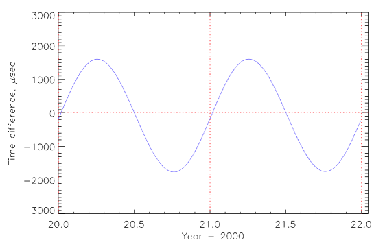
Figure 1: The time difference TCB–TCG, computed at the geocenter. The secular drift of 1.2794 ms/day has been removed.

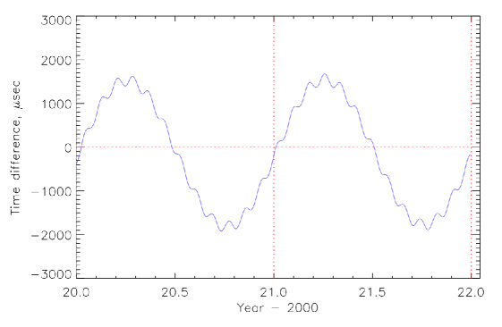
Figure 2: The time difference TCB–TCL, computed at the center of mass of the Moon. The secular drift of 1.2808 ms/day has been removed.

The result of the numerical integration of Eq. (12) for TCL–TCG is shown in Fig. 3, where a linear rate term of $\approx\!-1.5\;\mu\rm{s/day}$ has been removed (more on the rate below). For this integration, the point of reference is the center of mass of the Moon, so the last (non-integrated) term in Eq. (12) is zero.

Figure 3: Time difference TCL–TCG, with the secular drift removed, computed by evaluation of equation (12) at the Moon’s center of mass.

The integration covered 10 years at 0.1-day intervals, although only the first two years are shown in Figure 3. Note that the integral in Eq. (12) for TCL–TCG is the same as that in Eq. (25) for LT–TT, so that all the resulting periodic components from the integration of (12) appear in both transformations. The figure clearly shows the largest periodic term in the transformation shown in Eq. (86) (for $\mathcal{F}_{1}+\mathcal{F}_{2}$; $\mathcal{F}_{3}$ is zero in this case), which has an amplitude of $\approx\!0.5\;\mu\rm{s}$ and a period of 27.55 days. The power spectrum of the periodicities is shown in Fig. 4, with the periods of the largest components listed in (VIII.2) and (86) marked.

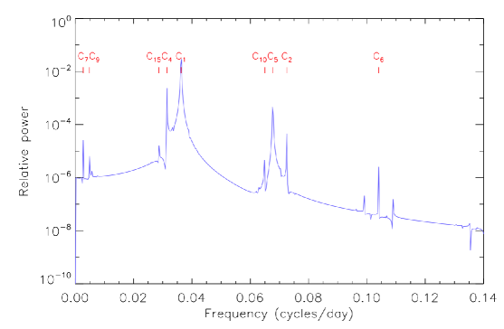
Figure 4: The power spectrum of periodicities in the integration result shown in Fig. 3.

Another numerical approach to obtaining TCL–TCG is to subtract the results of the separate integrations of Eqs. (1) and (2). However, in doing so it is important that a common point of reference, ${\bm{x}}$, be used. For ${\bm{x}}$ at the center of the Moon, i.e., ${\bm{x}}={\bm{x}}_{\scriptscriptstyle{\rm L}}$, the last (non-integrated) term in Eq. (1) must be evaluated but the corresponding term in Eq. (2) is zero. The overall difference between the coordinate times for the Moon and Earth time is then

$$s-u ={\rm(TCB-TCG)}({\bm{x}}_{L})-{\rm(TCB-TCL)}({\bm{x}_{L}})={\rm(TCL-TCG)}({\bm{x}_{L}})\;,$$ (97)

The result is identical to the result from integrating Eq. (12) except for a constant offset of $123.997\,\mu{\rm s}$, due to the different initializations in the two methods: all the integrations were arbitrarily set to zero at step 1 (on 2020 January 1), but Eq. (1) yields a non-zero value at step 1 due to the the term outside the integral. This independently validates Eq. (12).

If we extend the integration of Eq. (12) to 30 years and solve for the amplitudes of the 15 periodic components listed in (VIII.2), and compare them to the analytically obtained amplitudes given in Eq. (86), we obtain the results shown in Table 2.

Table 2. Major Periodic Components in TCL–TCG and LT–TT.
Symbol	Luni-solar	xxPeriod		Analytic	Numeric	Numeric
(this paper)	xargumentsx			xamplitudex	xamplitudex	uncertainty
		d0000		$\mu$s	$\mu$s	$\mu$s
$C_{1}$	$M$	27.5546		–0.4707	–0.4710	0.0003
$C_{2}$	$2M$	13.7773		–0.0130	–0.0128	0.0001
$C_{3}$	$3M$	9.1848		–0.0005	–0.0005	<0.0001<
$C_{4}$	$2D-M$	31.8119		–0.0814	–0.0927	0.0002
$C_{5}$	$2D$	14.7653		–0.0468	–0.0587	<0.0001<
$C_{6}$	$2D+M$	9.6137		–0.0025	–0.0035	0.0001
$C_{7}$	$M^{\prime}$	365.2596		- 0.0120	-0.0100	0.0002
$C_{8}$	$2F-2D$	173.3100		-.0.0005	-0.0013	0.0001
$C_{9}$	$2D-2M$	–205.8922		-.0.0009	–0.0046	0.0001
$C_{10}$	$2D-M^{\prime}$	15.3873		–0.0024	–0.0040	0.0001
$C_{11}$	$2D+M^{\prime}$	14.1916		–0.0003	-0.0006	0.0001
$C_{12}$	$M-M^{\prime}$	29.8028		–0.0016	—	—
$C_{13}$	$M+M^{\prime}$	25.6217		-.0.0016	-0.0023	0.0001
$C_{14}$	$2D-M+M^{\prime}$	29.2633		- 0.0011	—	—
$C_{15}$	$2D-M-M^{\prime}$	34.8469		–0.0025	–0.0041	0.0001

Here $M$ is the Moon’s mean anomaly, $M^{\prime}$ is the Earth’s mean anomaly, $D$ is the mean elongation of the Moon from the Sun, and $F$ is the difference between the mean longitude of the Moon and the longitude of the node of the lunar orbit ($F$ is also called the argument of latitude). Negative amplitudes indicate that the phase of the term is $\pm 180^{\circ}$ from that indicated by the arguments.

The formal uncertainties of the amplitudes from this 30-year solution are all <$0.0001\,\mu$s, and the phases were all very close to either 0 for positive amplitudes or $\pm 180^{\circ}$ for negative amplitudes. The uncertainties listed for each component in the last column are half the total range of amplitude values ($\frac{1}{2}$(max–min)) among five solutions involving 6-year subsets of the 30-year integration output, so they are more conservative than the formal errors. We did not obtain reliable solutions for $C_{12}$ or $C_{14}$ (the phases were inconsistent among solutions). The overall rate value computed in the same 30-year solution is $-1.4769\,\mu$s/day with an uncertainty of <$0.0001\,\mu$s/day, which can be compared to the analytical value of $C_{0}=-1.4714\,\mu$s/day given in Eq. (85).

Due to the complexity of the lunar orbit, the table is undoubtedly incomplete. Removing the rate term and these 15 components from the integration output leaves a TCL–TCG time series that remains within a range of $\pm 7$ ns and that shows evidence of other small periodicities.

IX.2 Clocks on the surfaces of the Earth and Moon

The ultimate objective is to compare the proper time kept by hypothesized real clocks on the surfaces of the Moon and Earth, i.e., a comparison of proper times as given by Eqs. (25), (26), and (27). If we limit the discussion here to clocks on the reference equipotential surfaces, the geoid for the Earth and the selenoid for the Moon, then by Eqs. (26) and (27), the proper times are TT for the Earth clock and LT for the Moon clock. Note that there has been no international agreement on the definition of the selenoid (which may vary by lunar gravity model), so the precise rate of LT with respect to the coordinate time TCL may need some future adjustment.

The integrals in Eq. (25) have already been evaluated, since their sum is the same as the integral in Eq. (12), the computation of which was described in the previous subsection. The results were described by a secular drift of $-1.4769\,\mu$s/day and the periodic terms in Table 2. Call that secular drift rate $L_{\scriptscriptstyle{\rm{TCL-TCG}}}$; then the total rate difference between the Earth and Moon clocks is $L_{\scriptscriptstyle{\rm E}}-L_{\scriptscriptstyle{\rm L}}-L_{\scriptscriptstyle{\rm{TCL-TCG}}}=60.2147-2.7128-1.4769=56.025\,\mu$s/day (TT day), using the rates for $L_{\scriptscriptstyle{\rm E}}$ and $L_{\scriptscriptstyle{\rm L}}$ given in Eqs. (21) and (22). The lunar clock runs faster than the terrestrial one by that amount, as a long-term average.

With the secular drift rate of proper time on the lunar surface with respect to the proper time on the Earth’s geoid established, as well as the periodic terms given in Table 2 from the difference in the coordinate times at the center of mass of the Moon, the problem of comparing real clocks on the Earth and Moon reverts to the evaluation of the small location-dependent component of TCL–TCG, or LT–TT, given by the last (non-integrated) term in Eq. (25). This component is approximated by the function $\mathcal{F}_{3}$ in the analytic development in Section VIII.3 and involves a few nanosecond-level periodic components but no additional rate changes.

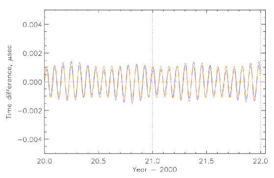
Figure 5: Difference in time between TCL on the selenoid at a location near the center of the Moon’s disk as seen from Earth (lunar longitude $l=0^{\circ}$, latitude $b=0^{\circ}$) and TCL at the Moon’s center of mass. The location-dependent term in (25), evaluated using the JPL ephemerides, is shown in blue and the analytic approximation $\mathcal{F}_{3}$ is shown in orange.

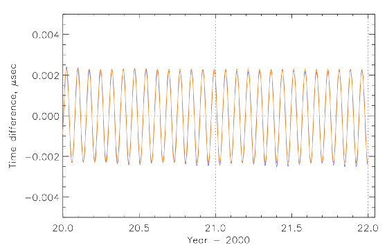
Figure 6: Same as Figure 5, but for a clock at the lunar south pole. The two curves overlap almost exactly at this location.

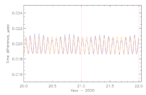
Figure 7: Same as Figure 5, but for a clock at the Moon’s eastern limb (lunar longitude $l=90^{\circ}$, latitude $b=0^{\circ}$).

Evaluating the location-dependent term in Eq. (25), using the lunar velocity and orientation data from the JPL DE440 ephemeris, we obtain Figs. 5, 6, and 7 for clocks at the center of the disk (longitude $l=0^{\circ}$, latitude $b=0^{\circ}$), the lunar south pole, and the eastern limb at the equator (longitude $l=90^{\circ}$, latitude $b=0^{\circ}$), respectively. These plots also show the curves representing the expression (96) for $\mathcal{F}_{3}$. The center of disk location (Figure 5) is sensitive to only the second term in (96); the south pole location (Figure 6) is sensitive to only the last term; and the equatorial limb location (Figure 7) is sensitive to both the first and second terms. As can be seen, the analytic expression well represents the numerical results.

X Conclusion

The current decade will see increasing operations, both human and robotic, on the lunar surface and in orbit around the Moon. A precise time standard, or standards, for the Moon will be necessary to enable such basic capabilities as navigation, selenodesy, secure communications, and many types of scientific measurements [2].

We have examined the relativistic differences between hypothetical clocks on the Moon and Earth. A Lunar Celestial Reference System has been described that is analogous to the Geocentric Celestial Reference System now used for precise applications on the Earth and in the near-Earth environment. TCL, a proposed lunar coordinate time for the LCRS, runs slow compared to TCG, geocentric coordinate time, by $1.477\,\mu\rm{s}/\rm{day}$ as a long-term average. However, periodic variations at several amplitudes and frequencies, including a monthly component with an amplitude of $0.5\,\mu\rm{s}$, are also present. LT, the proper time of a clock on the lunar surface (i.e., at the adopted lunar radius), would run systematically fast compared to TT, the proper time of a clock on the Earth’s surface (on the adopted Earth geoid), by $56.025\,\mu\rm{s}/\rm{day}$ as a long-term average. The periodic variations that appear in the comparison of the two coordinate times are also present in the comparison of the two proper times, LT and TT, and may be significant for some practical applications.

Satellite navigation systems require satellite clocks that are synchronized to $\approx$ $30\,\rm{ns}$ for $\approx$ $10\,\rm{m}$ positioning accuracy, and that duplicate, at the same level of accuracy, a ground-based time standard that is used by the control system. For such a system for the Moon, this means that the satellite clocks must be synchronized within the LCRS, in TCL or a constant-rate-difference substitute for TCL, i.e,

$$t_{\rm nav}={\rm TCL}\times(1+r_{\rm nav})+\Delta t_{0}\;,$$

where $r_{\rm nav}$ is the fractional rate offset ($|r_{\rm nav}|\ll 1$), and $\Delta t_{0}$ is an epoch difference. That is, whatever time scale is used for navigation must advance by seconds that have a known and fixed relation to SI seconds at the origin of the LCRS. Note, however, that the use of any time scale for the LCRS that does not have the same rate as TCL would necessitate a re-scaling of the meter. Furthermore, any astronomical constant present in equations where the meter is used as a dimension would also need to be recalibrated [41, 42].

The differences between LT and TT described in this paper apply to any clock on the Moon that is set up to distribute Earth time. Any clock system on the Moon that compensates in some way for the periodic variations described in Table 2 would produce seconds that would not have a constant length at the Moon. For example, the $C_{1}$ periodic component represents a maximum variation of 0.2% in the LT–TT clock rate difference, and a maximum fractional variation in the length of a lunar second of $\sim\!10^{-12}$. Although this appears to be a small number, it is orders of magnitude larger than the precision of the best modern atomic clocks. This is an issue that may not be important for most ordinary lunar applications, but that would be a consideration for those in the future requiring very precise time or metrology.

Appendix A The Earth-Moon Local Coordinate System and Lunar Time

In a recent scientific paper, Ashby and Patla [5] propose a framework that addresses the establishment and dissemination of Coordinated Universal Time (UTC) from Earth to the Moon and beyond. Their approach utilizes a metric that is appropriate for a locally freely falling Earth-Moon system. The approach by Ashby and Patla [5] to the lunar time (LT) diverges from the formalism of local inertial coordinates, which is based on the IAU 2000 resolutions [9] adopted in the present paper. Notably, it leads to the establishment of the LT–TT relationship [5, Section 3] that appears to differ formally from the result we obtained in Eq. (25).

The primary objective of this appendix is threefold:

1. Extension of IAU 2000 resolutions on time scales: We aim to extend the IAU time resolutions to encompass the Earth-Moon system.

2. Comparison with the Ashby and Patla [5] approach: We demonstrate that the LT–TT relationship derived through this extension not only reproduces but also generalizes the approach in Ashby and Patla [5].

3. Comparison with the standard approach based on the IAU 2000 resolutions: We demonstrate that the extended and standard approaches to establishing the coordinate time on the Moon lead to the identical LT–TT relationship and are interconvertible. It ensures consistency in timekeeping and facilitates seamless communication and navigation between Earth and the Moon.

Throughout of the appendix we use some additional notations. Spatial vector and/or tensor indices $i,j,k$ take values 1,2,3. We use a multi-index tensor notation for space tensors, for example, a tensor $Q_{K}:=Q_{i_{1}i_{2}...i_{k}}$, a tensor $X^{K}:=X^{i_{1}i_{2}...i_{k}}=X^{i_{1}}X^{i_{2}}...X^{i_{l}}$. By the symbol $\partial_{i}$ we denote a partial derivative with respect to the $i$-th spatial coordinate. Multi-index notations are also used for high-order partial derivatives, for example, a partial derivative of the order $k$ is denoted as $\partial_{K}:=\partial_{i_{1}i_{2}...i_{k}}$. A repeated spatial index represents a summation from 1 to 3, that is, $A_{i}B^{i}=A_{1}B^{1}+A_{2}B^{2}+A_{3}B^{3}$.

A.1 Extension of IAU 2000 time resolutions to the Earth-Moon system

The IAU 2000 resolutions concerning astronomical reference systems focus on two distinct coordinate systems within the solar system: the Barycentric Celestial Reference System (BCRS) and the Geocentric Celestial Reference System (GCRS) and their respective coordinate times, TCB and TCG. The BCRS serves as a global coordinate chart that spans the entire spacetime. It provides a framework for precise astronomical measurements and calculations. Importantly, the BCRS metric takes into account the gravitational influence of all massive bodies in the solar system. The GCRS, in contrast, represents an example of local inertial coordinates. It is constructed in the vicinity of a single massive body: our planet, Earth. Within this framework, the Moon is treated as one of the massive external bodies in the solar system. The Moon’s orbital motion is considered on equal terms with Earth’s orbital motion around the solar system barycenter.

However, the Moon is gravitationally bound to Earth and is an integral part of the Earth-Moon system. This system is in a state of free fall within the gravitational field of the Sun and other massive bodies in our solar system. In certain relativistic applications (such as establishing lunar time or conducting lunar laser ranging), where we need to treat the Moon as a massive body, it is more natural to extend the IAU reference system concepts to encompass the Earth-Moon system as a whole. To achieve this, we introduce an intermediate Earth-Moon coordinate chart, specifically designed for the Earth-Moon system and centered at the system’s center of mass.

Let us denote the Earth-Moon coordinate reference system (EMCRS) as $(T,{\bm{X}})$ where $T$ represents the new time coordinate and ${\bm{X}}=(X^{i})=(X^{1},X^{2},X^{3})$ are the spatial coordinates aligned with the coordinate axes of the BCRS. The EMCRS metric tensor accounts for the gravitational interaction between Earth and Moon. A detailed relativistic description of the EMCRS, including its metric tensor, is provided in the work by [3]. This paper also establishes the connection between the EMCRS and other reference systems such as the BCRS, GCRS, and LCRS. By introducing the intermediate time scale $T$ associated with the Earth-Moon system, we can establish the lunar coordinate time (TCL) and explore the TCL–TCG time transformation from a different perspective.

Firstly, let’s establish the transformation between the time $T$ of the Earth-Moon system and $t=$TCB (Barycentric Coordinate Time). The derivation of this transformation relies upon the same guiding principles of the IAU resolutions as the derivation of the transformation between TCG (Geocentric Coordinate Time) and TCB. However, in this case, we replace the Earth with the Earth-Moon system. The relevant equation is given as follows [3, Eq. 5.24] (notice that designations used for time and space coordinates in paper [3] differ from the present paper):

$$T = t-\frac{1}{c^{2}}\int\limits_{t_{0}}^{t}\left[\frac{v_{\scriptscriptstyle{\rm B}}^{2}}{c^{2}}+\hbox to0.0pt{\hskip 1.459pt\leavevmode\hbox{\set@color$\overline{\hbox{}}$}\hss}{\leavevmode\hbox{\set@color$U$}}\left({\bm{x}}_{\scriptscriptstyle{\rm B}}\right)\right]dt-\frac{1}{c^{2}}{\bm{v}}_{\scriptscriptstyle{\rm B}}\cdot{\bm{r}}_{\scriptscriptstyle{\rm B}}\;,$$ (98)

where

$$\hbox to0.0pt{\hskip 1.459pt\leavevmode\hbox{\set@color$\overline{\hbox{}}$}\hss}{\leavevmode\hbox{\set@color$U$}}\left({\bm{x}}\right) = \sum_{{\scriptscriptstyle{\rm A}}\neq{\scriptscriptstyle{\rm E}},{\scriptscriptstyle{\rm L}}}\frac{\mu_{\scriptscriptstyle{\rm A}}}{r_{{\scriptscriptstyle{\rm A}}}}\;,$$ (99)

is the gravitational potential of the external bodies taken at the point ${\bm{x}}={\bm{x}}_{\scriptscriptstyle{\rm B}}$, $r_{A}=|{\bm{r}}_{\scriptscriptstyle{\rm A}}|$, and ${\bm{r}}_{\scriptscriptstyle{\rm A}}={\bm{x}}-{\bm{x}}_{\scriptscriptstyle{\rm A}}$. Notice that both Earth and Moon have been excluded from the potential  $\overline{\hbox{}}$$U$. Transformation of the spatial coordinates of the BCRS and EMCRS is given by a simple translation of the coordinate origin

$${\bm{X}}={\bm{x}}-{\bm{x}}_{\scriptscriptstyle{\rm B}}\;,$$ (100)

where ${\bm{x}}_{\scriptscriptstyle{\rm B}}$ are the BCRS coordinates of the center of mass of the Earth-Moon system. In what follows, two EMCRS vectors will be important: (1) the radius vector of the Earth’s center of mass, ${\bm{X}}_{\scriptscriptstyle{\rm E}}={\bm{x}}_{\scriptscriptstyle{\rm E}}-{\bm{x}}_{\scriptscriptstyle{\rm B}}$, and (2) the radius vector of the Moon’s center of mass, ${\bm{X}}_{\scriptscriptstyle{\rm L}}={\bm{x}}_{\scriptscriptstyle{\rm L}}-{\bm{x}}_{\scriptscriptstyle{\rm B}}$. It is worth noting that the EMCRS spatial vector ${\bm{X}}_{{\scriptscriptstyle{\rm L}}{\scriptscriptstyle{\rm E}}}$ is equivalent to the geocentric radius-vector of the Moon ${\bm{r}}_{{\scriptscriptstyle{\rm L}}{\scriptscriptstyle{\rm E}}}$, that is ${\bm{X}}_{{\scriptscriptstyle{\rm L}}{\scriptscriptstyle{\rm E}}}={\bm{r}}_{{\scriptscriptstyle{\rm L}}{\scriptscriptstyle{\rm E}}}$ which can be checked by inspection.

Both the GCRS and LCRS exists in a state of free fall with respect to the barycenter of the Earth-Moon system. Since the Earth and Moon are gravitationally bound, the rate of the E-clock on the Earth is subject to the direct influence of the gravitational potential of the Moon. However, because the Earth-Moon system is itself in a state of free fall with respect to the barycenter of the solar system, the gravitational field of other bodies of the solar system can appear only in the form of a tidal potential. Hence, the time transformation between $u=$TCG (Geocentric Coordinate Time) and the coordinate time $T$ of the Earth-Moon coordinate system takes on the following form [3, Eq. 5.63]:

$$u = T-\frac{1}{c^{2}}\int\limits_{T_{0}}^{T}\left[\frac{V_{\scriptscriptstyle{\rm E}}^{2}}{2}+\frac{\mu_{\scriptscriptstyle{\rm L}}}{R_{{\scriptscriptstyle{\rm L}}{\scriptscriptstyle{\rm E}}}}+Q_{i}X^{i}_{\scriptscriptstyle{\rm E}}+\sum_{k=2}^{\infty}\frac{1}{k!}Q_{K}X^{K}_{\scriptscriptstyle{\rm E}}\right]dT-\frac{1}{c^{2}}{\bm{V}}_{\scriptscriptstyle{\rm E}}\cdot{\bm{R}}_{\scriptscriptstyle{\rm E}}\;,$$ (101)

where ${\bm{V}}_{\scriptscriptstyle{\rm E}}=\dot{\bm{X}}_{\scriptscriptstyle{\rm E}}$ is the velocity of the geocenter with respect to the barycenter of the Earth-Moon system, ${\bm{X}}_{\scriptscriptstyle{\rm E}}=(X^{i}_{\scriptscriptstyle{\rm E}})$ represents the EMCRS coordinate of the geocenter, ${\bm{R}}_{\scriptscriptstyle{\rm E}}={\bm{X}}-{\bm{X}}_{\scriptscriptstyle{\rm E}}={\bm{r}}_{\scriptscriptstyle{\rm E}}$ is the radius-vector from the geocenter to the point of measurement of TCG, and ${\bm{R}}_{{\scriptscriptstyle{\rm L}}{\scriptscriptstyle{\rm E}}}={\bm{X}}_{\scriptscriptstyle{\rm L}}-{\bm{X}}_{\scriptscriptstyle{\rm E}}={\bm{r}}_{{\scriptscriptstyle{\rm L}}{\scriptscriptstyle{\rm E}}}$ is the radius-vector from geocenter to the center of mass of the Moon.

Equation (101) contains additional parameters compared to the transformation between TCG and TCB. They include the dipole moment, $Q_{i}$, and higher-order external multipole moments, $Q_{K}:=Q_{i_{1}i_{2}...i_{k}}$ ($k\leq 2$). The dipole moment $Q_{i}$ is interconnected to the high-order multipoles by the constraint that the linear momentum of the Earth-Moon system vanishes in the local EMCRS coordinates [10, Section 6.1.4]. We obtain

$$Q_{i} = \-\left(M_{\scriptscriptstyle{\rm E}}+M_{\scriptscriptstyle{\rm L}}\right)^{-1}\sum_{k=1}^{\infty}Q_{ii_{1}i_{2}...i_{k}}M^{i_{1}i_{2}...i_{k}}\;,$$ (102)

where $M^{i_{1}i_{2}...i_{k}}$ are the intrinsic multipole moments of the gravitational field of the Earth-Moon system:

$$M^{i_{1}i_{2}...i_{k}} = M_{\scriptscriptstyle{\rm E}}X_{\scriptscriptstyle{\rm E}}^{i_{1}i_{2}...i_{k}}+M_{\scriptscriptstyle{\rm L}}X_{\scriptscriptstyle{\rm L}}^{i_{1}i_{2}...i_{k}}\qquad\quad(k\geq 2)\;.$$ (103)

Thus, physical significance of the dipole moment $Q_{i}$ is that it describes how the combined center of mass of the Earth and Moon (the Earth-Moon barycenter) accelerates relative to a hypothetical particle which is moving freely along a path (called a timelike geodesic) in the gravitational field created by the Sun and other large bodies in the solar system. The acceleration is caused by the gravitational coupling of the intrinsic multipole moments of the Earth-Moon system $M^{i_{1}i_{2}...i_{k}}$ with the external multipole moments of tidal gravitational field of the external bodies of the solar system, which are defined in terms of the partial derivatives

$$Q_{i_{1}i_{2}...i_{k}} = \partial_{i_{1}i_{2}...i_{k}}{\hbox to0.0pt{\hskip 1.459pt\leavevmode\hbox{\set@color$\overline{\hbox{}}$}\hss}{\leavevmode\hbox{\set@color$U$}}}({\bm{x}}_{\scriptscriptstyle{\rm B}})\;,$$ (104)

of the external gravitational field of the solar system bodies computed at the barycenter of the Earth-Moon system. The motion of the center of mass of the Earth-Moon system with respect to BCRS obeys the equations of motion

$$a^{i}_{\scriptscriptstyle{\rm B}} = \partial_{i}{\hbox to0.0pt{\hskip 1.459pt\leavevmode\hbox{\set@color$\overline{\hbox{}}$}\hss}{\leavevmode\hbox{\set@color$U$}}}({\bm{x}}_{\scriptscriptstyle{\rm B}})-Q_{i}\;.$$ (105)

where $(a^{i}_{\scriptscriptstyle{\rm B}})={\bm{a}}_{\scriptscriptstyle{\rm B}}=\ddot{\bm{x}}_{\scriptscriptstyle{\rm B}}$ is the BCRS coordinate acceleration of the Earth-Moon barycenter.

Similar arguments are applied to the derivation of the time transformation between TCL$=s$ and the coordinate time $T$ of the Earth-Moon system. We have [3, Eq. 5.78]

$$s = T-\frac{1}{c^{2}}\int\limits_{T_{0}}^{T}\left[\frac{V_{\scriptscriptstyle{\rm L}}^{2}}{2}+\frac{\mu_{\scriptscriptstyle{\rm E}}}{R_{{\scriptscriptstyle{\rm L}}{\scriptscriptstyle{\rm E}}}}+Q_{i}X^{i}_{\scriptscriptstyle{\rm L}}+\sum_{k=2}^{\infty}\frac{1}{k!}Q_{K}X^{K}_{\scriptscriptstyle{\rm L}}\right]dT-\frac{1}{c^{2}}{\bm{V}}_{\scriptscriptstyle{\rm L}}\cdot{\bm{R}}_{\scriptscriptstyle{\rm L}}\;,$$ (106)

where ${\bm{X}}_{\scriptscriptstyle{\rm L}}=(X^{i}_{\scriptscriptstyle{\rm L}})$ is the EMCRS coordinate of the Moon’s center of mass, ${\bm{V}}_{\scriptscriptstyle{\rm L}}=\dot{\bm{X}}_{\scriptscriptstyle{\rm L}}$ is the velocity of the Moon with respect to the barycenter of the Earth-Moon system, ${\bm{R}}_{\scriptscriptstyle{\rm L}}={\bm{X}}-{\bm{X}}_{\scriptscriptstyle{\rm L}}={\bm{r}}_{\scriptscriptstyle{\rm L}}$ is the radius-vector from the center of mass of the Moon to the point of measurement of TCL, and the dipole moment $Q_{i}$ is given in Eq. (102) and the multipole moments $Q_{K}$ in Eq. (104).

The infinite sums appearing in Eqs. (101) and (106) can be considered part of the Taylor expansion of the gravitational potential $\hbox to0.0pt{\hskip 1.459pt\leavevmode\hbox{\set@color$\overline{\hbox{}}$}\hss}{\leavevmode\hbox{\set@color$U$}}({\bm{x}})$ of the external bodies with the center of the expansion taken at different points of space. Indeed, it is straightforward to confirm that

$$\sum_{k=2}^{\infty}\frac{1}{k!}Q_{K}X^{K}_{\scriptscriptstyle{\rm E}} = {\hbox to0.0pt{\hskip 1.459pt\leavevmode\hbox{\set@color$\overline{\hbox{}}$}\hss}{\leavevmode\hbox{\set@color$U$}}}({\bm{x}}_{\scriptscriptstyle{\rm E}})-\hbox to0.0pt{\hskip 1.459pt\leavevmode\hbox{\set@color$\overline{\hbox{}}$}\hss}{\leavevmode\hbox{\set@color$U$}}({\bm{x}}_{\scriptscriptstyle{\rm B}})-X^{i}_{\scriptscriptstyle{\rm E}}\partial_{i}\hbox to0.0pt{\hskip 1.459pt\leavevmode\hbox{\set@color$\overline{\hbox{}}$}\hss}{\leavevmode\hbox{\set@color$U$}}({\bm{x}}_{\scriptscriptstyle{\rm B}})\;,$$ (107)

$$\sum_{k=2}^{\infty}\frac{1}{k!}Q_{K}X^{K}_{\scriptscriptstyle{\rm L}} = {\hbox to0.0pt{\hskip 1.459pt\leavevmode\hbox{\set@color$\overline{\hbox{}}$}\hss}{\leavevmode\hbox{\set@color$U$}}}({\bm{x}}_{\scriptscriptstyle{\rm L}})-\hbox to0.0pt{\hskip 1.459pt\leavevmode\hbox{\set@color$\overline{\hbox{}}$}\hss}{\leavevmode\hbox{\set@color$U$}}({\bm{x}}_{\scriptscriptstyle{\rm B}})-X^{i}_{\scriptscriptstyle{\rm L}}\partial_{i}\hbox to0.0pt{\hskip 1.459pt\leavevmode\hbox{\set@color$\overline{\hbox{}}$}\hss}{\leavevmode\hbox{\set@color$U$}}({\bm{x}}_{\scriptscriptstyle{\rm B}})\;.$$ (108)

Subtracting (101) from (106) cancels out the coordinate time $T$ and leads to a new equation that describes the relationship between TCL (Lunar Coordinate Time) and TCG (Geocentric Coordinate Time)

$$s = u-\frac{1}{c^{2}}\int\limits_{T_{0}}^{T}\left[\frac{V_{\scriptscriptstyle{\rm L}}^{2}-V_{\scriptscriptstyle{\rm E}}^{2}}{2}+\frac{\mu_{\scriptscriptstyle{\rm E}}-\mu_{\scriptscriptstyle{\rm L}}}{r_{{\scriptscriptstyle{\rm L}}{\scriptscriptstyle{\rm E}}}}+\hbox to0.0pt{\hskip 1.459pt\leavevmode\hbox{\set@color$\overline{\hbox{}}$}\hss}{\leavevmode\hbox{\set@color$U$}}({\bm{x}}_{\scriptscriptstyle{\rm L}})-\hbox to0.0pt{\hskip 1.459pt\leavevmode\hbox{\set@color$\overline{\hbox{}}$}\hss}{\leavevmode\hbox{\set@color$U$}}({\bm{x}}_{\scriptscriptstyle{\rm E}})+r_{{\scriptscriptstyle{\rm L}}{\scriptscriptstyle{\rm E}}}^{i}Q_{i}-r_{{\scriptscriptstyle{\rm L}}{\scriptscriptstyle{\rm E}}}^{i}\partial_{i}\hbox to0.0pt{\hskip 1.459pt\leavevmode\hbox{\set@color$\overline{\hbox{}}$}\hss}{\leavevmode\hbox{\set@color$U$}}({\bm{x}}_{\scriptscriptstyle{\rm B}})\right]dT$$ (109)

$$\leavevmode\nobreak\ \leavevmode\nobreak\ -\frac{1}{c^{2}}\left({\bm{V}}_{\scriptscriptstyle{\rm L}}\cdot{\bm{r}}_{\scriptscriptstyle{\rm L}}-{\bm{V}}_{\scriptscriptstyle{\rm E}}\cdot{\bm{r}}_{\scriptscriptstyle{\rm E}}\right),$$

where $(r_{{\scriptscriptstyle{\rm L}}{\scriptscriptstyle{\rm E}}}^{i})={\bm{r}}_{{\scriptscriptstyle{\rm L}}{\scriptscriptstyle{\rm E}}}={\bm{X}}_{{\scriptscriptstyle{\rm L}}{\scriptscriptstyle{\rm E}}}$ is the radius-vector of the Moon with respect to the Earth’s geocenter. This equation can be elaborated further by expanding the gravitational potential $\hbox to0.0pt{\hskip 1.459pt\leavevmode\hbox{\set@color$\overline{\hbox{}}$}\hss}{\leavevmode\hbox{\set@color$U$}}({\bm{x}}_{\scriptscriptstyle{\rm L}})$ in a Taylor series around the point ${\bm{x}}_{\scriptscriptstyle{\rm E}}$. This yields

$$s = u-\frac{1}{c^{2}}\int\limits_{T_{0}}^{T}\left[\frac{V_{\scriptscriptstyle{\rm L}}^{2}-V_{\scriptscriptstyle{\rm E}}^{2}}{2}+\frac{\mu_{\scriptscriptstyle{\rm E}}-\mu_{\scriptscriptstyle{\rm L}}}{r_{{\scriptscriptstyle{\rm L}}{\scriptscriptstyle{\rm E}}}}+W({\bm{x}}_{\scriptscriptstyle{\rm E}})+r_{{\scriptscriptstyle{\rm L}}{\scriptscriptstyle{\rm E}}}^{i}Q_{i}+r_{{\scriptscriptstyle{\rm L}}{\scriptscriptstyle{\rm E}}}^{i}\partial_{i}\hbox to0.0pt{\hskip 1.459pt\leavevmode\hbox{\set@color$\overline{\hbox{}}$}\hss}{\leavevmode\hbox{\set@color$U$}}({\bm{x}}_{\scriptscriptstyle{\rm E}})-r_{{\scriptscriptstyle{\rm L}}{\scriptscriptstyle{\rm E}}}^{i}\partial_{i}\hbox to0.0pt{\hskip 1.459pt\leavevmode\hbox{\set@color$\overline{\hbox{}}$}\hss}{\leavevmode\hbox{\set@color$U$}}({\bm{x}}_{\scriptscriptstyle{\rm B}})\right]dT$$ (110)

$$\leavevmode\nobreak\ \leavevmode\nobreak\ -\frac{1}{c^{2}}\Bigl{(}{\bm{V}}_{\scriptscriptstyle{\rm L}}\cdot{\bm{r}}_{\scriptscriptstyle{\rm L}}-{\bm{V}}_{\scriptscriptstyle{\rm E}}\cdot{\bm{r}}_{\scriptscriptstyle{\rm E}}\Bigr{)}\;,$$

where the perturbing tidal potential of the external bodies

$$W({\bm{x}}_{\scriptscriptstyle{\rm E}}) := \sum_{k=2}\frac{1}{k!}\partial_{i_{1}i_{2}...i_{k}}\hbox to0.0pt{\hskip 1.459pt\leavevmode\hbox{\set@color$\overline{\hbox{}}$}\hss}{\leavevmode\hbox{\set@color$U$}}({\bm{x}}_{\scriptscriptstyle{\rm E}})r_{{\scriptscriptstyle{\rm L}}{\scriptscriptstyle{\rm E}}}^{i_{1}i_{2}...i_{k}}\;,$$ (111)

is computed at the geocenter. Finally, we expand the difference between the two last terms in the integrand of Eq. (110) in the Taylor series

$$r_{{\scriptscriptstyle{\rm L}}{\scriptscriptstyle{\rm E}}}^{i}\partial_{i}\hbox to0.0pt{\hskip 1.459pt\leavevmode\hbox{\set@color$\overline{\hbox{}}$}\hss}{\leavevmode\hbox{\set@color$U$}}({\bm{x}}_{\scriptscriptstyle{\rm E}})-r_{{\scriptscriptstyle{\rm L}}{\scriptscriptstyle{\rm E}}}^{i}\partial_{i}\hbox to0.0pt{\hskip 1.459pt\leavevmode\hbox{\set@color$\overline{\hbox{}}$}\hss}{\leavevmode\hbox{\set@color$U$}}({\bm{x}}_{\scriptscriptstyle{\rm B}}) = \sum_{k=1}\frac{1}{k!}Q_{iK}X^{K}_{\scriptscriptstyle{\rm E}}\;,$$ (112)

and express the coordinate times $s=$TCL and $u=$TCG in terms of proper times LT and TT measured on selenoid and geoid, respectively, by means of Eqs. (19), (20). It allows us to present Eq. (110) in the following form:

$${\rm LT} = \left(1+L_{\scriptscriptstyle{\rm E}}-L_{\scriptscriptstyle{\rm L}}\right){\rm TT}-\frac{1}{c^{2}}\int\limits_{t_{0}}^{t}\left[\frac{1}{2}\left(V_{\scriptscriptstyle{\rm L}}^{2}-V_{\scriptscriptstyle{\rm E}}^{2}\right)+\frac{\mu_{\scriptscriptstyle{\rm E}}-\mu_{\scriptscriptstyle{\rm L}}}{r_{{\scriptscriptstyle{\rm L}}{\scriptscriptstyle{\rm E}}}}+W({\bm{x}}_{\scriptscriptstyle{\rm E}})+r_{{\scriptscriptstyle{\rm L}}{\scriptscriptstyle{\rm E}}}^{i}\left(Q_{i}+\sum_{k=1}\frac{1}{k!}Q_{iK}X^{K}_{\scriptscriptstyle{\rm E}}\right)\right]dt$$ (113)

$$\phantom{\left(1+L_{\scriptscriptstyle{\rm E}}-L_{\scriptscriptstyle{\rm L}}\right){\rm TT}}-\frac{1}{c^{2}}\Bigl{(}{\bm{V}}_{\scriptscriptstyle{\rm L}}\cdot{\bm{r}}_{\scriptscriptstyle{\rm L}}-{\bm{V}}_{\scriptscriptstyle{\rm E}}\cdot{\bm{r}}_{\scriptscriptstyle{\rm E}}\Bigr{)}\;,$$

where we have replaced integration with respect to time $T$ with integration with respect to TCB time $t$, because the difference between these two time scales is of the post-Newtonian order of magnitude and can be neglected.

Equation (113) is fundamental in the extension of the IAU time resolutions to the Earth-Moon system. It expresses the lunar time in terms of the terrestrial time which is directly connected to UTC, and all quantities entering the LT–TT transformation are measured by a fictitious observer who is at rest with respect to the Earth-Moon barycenter. It is like having a clock that works the same way whether you are on the Earth or the Moon.

A.2 Comparison with the Ashby and Patla approach

The fundamental time transformation Eq. (113) can be compared to the corresponding equation derived by Ashby and Patla [5]. These authors considered the fractional frequency shift of two atomic clocks counting the lunar and terrestrial time, but they neglected all tidal terms that appear in Eq. (113) under the sign of the integral. The proper time of the L-clock on the Moon, $\tau_{\scriptscriptstyle{\rm L}}$, and the proper time of the E-clock on Earth, $\tau_{\scriptscriptstyle{\rm E}}$, are linear functions of the lunar time LT and terrestrial time TT, respectively, as evident from Eqs. (26), (27). Making use of these equations and differentiating Eq. (113), with all tidal and multipole-moment terms discarded, we obtain

$$\frac{d\tau_{\scriptscriptstyle{\rm L}}-d\tau_{\scriptscriptstyle{\rm E}}}{d\tau_{\scriptscriptstyle{\rm E}}} = -\frac{1}{2c^{2}}\Bigl{(}V^{2}_{\scriptscriptstyle{\rm L}}-V^{2}_{\scriptscriptstyle{\rm E}}\Bigr{)}+\frac{\mu_{\scriptscriptstyle{\rm L}}-\mu_{\scriptscriptstyle{\rm E}}}{c^{2}r_{{\scriptscriptstyle{\rm L}}{\scriptscriptstyle{\rm E}}}}+\frac{\Phi_{0{\scriptscriptstyle{\rm E}}}-\Phi_{0{\scriptscriptstyle{\rm L}}}}{c^{2}}$$

$$-\frac{1}{c^{2}}\Bigl{(}{\bm{A}}_{\scriptscriptstyle{\rm L}}\cdot{\bm{z}}-{\bm{A}}_{\scriptscriptstyle{\rm E}}\cdot{\bm{w}}\Bigr{)}-\frac{1}{c^{2}}\Bigl{(}{\bm{V}}_{\scriptscriptstyle{\rm L}}\cdot\dot{\bm{z}}-{\bm{V}}_{\scriptscriptstyle{\rm E}}\cdot\dot{\bm{w}}\Bigr{)}\;,$$

where the notation for the selenocentric (LCRS) coordinates ${\bm{z}}={\bm{r}}_{\scriptscriptstyle{\rm L}}$ and that for the geocentric (GCRS) coordinates ${\bm{w}}={\bm{r}}_{\scriptscriptstyle{\rm E}}$ of the atomic clocks have been used, and ${\bm{A}}_{\scriptscriptstyle{\rm E}}=\dot{\bm{V}}_{\scriptscriptstyle{\rm E}}$ and ${\bm{A}}_{\scriptscriptstyle{\rm L}}=\dot{\bm{V}}_{\scriptscriptstyle{\rm L}}$ are the coordinate accelerations of the Earth and Moon with respect to the barycenter of the Earth-Moon system. Terms in the first line of the right hand-side of Eq. (A.2) coincide with the terms given by Ashby and Patla [5] in their equation (18), while the terms from the second line of Eq. (A.2) appear in equations (29), (32) and (33) of their paper. This highlights a valuable correspondence between the paper by Ashby and Patla [5] and the extended IAU 2000 resolutions on time scales described in this appendix. The extended IAU 2000 framework provides a more fundamental approach to the time scales in the Earth-Moon system by accounting not only for the kinematic (motion-related) effects and those from the gravitational field of the Earth and Moon, but it also includes a comprehensive description of the tidal effects on the time transformations, which helps us to better understand how we measure time.

A.3 Comparison with the standard approach based on the IAU 2000 resolutions

Let us compare Eq. (113) with Eq. (25), which has been obtained in the main body of the present paper without introducing the intermediate local coordinates attached to the barycenter of the Earth-Moon system. The kinematic (velocity-dependent) term under the sign of integral in Eq. (113) can be decomposed into three terms:

$$\frac{V_{\scriptscriptstyle{\rm L}}^{2}-V_{\scriptscriptstyle{\rm E}}^{2}}{2} = \frac{v_{{\scriptscriptstyle{\rm L}}{\scriptscriptstyle{\rm E}}}^{2}}{2}-{\bm{A}}_{\scriptscriptstyle{\rm E}}\cdot{\bm{r}}_{{\scriptscriptstyle{\rm L}}{\scriptscriptstyle{\rm E}}}+\frac{d}{dT}\Bigl{(}{\bm{V}}_{\scriptscriptstyle{\rm E}}\cdot{\bm{r}}_{{\scriptscriptstyle{\rm L}}{\scriptscriptstyle{\rm E}}}\Bigr{)}\;,$$ (115)

where ${\bm{r}}_{{\scriptscriptstyle{\rm L}}{\scriptscriptstyle{\rm E}}}:={\bm{X}}_{\scriptscriptstyle{\rm L}}-{\bm{X}}_{\scriptscriptstyle{\rm E}}={\bm{x}}_{\scriptscriptstyle{\rm L}}-{\bm{x}}_{\scriptscriptstyle{\rm E}}$ is the radius-vector of the Moon with respect to Earth’s geocenter, ${\bm{v}}_{{\scriptscriptstyle{\rm L}}{\scriptscriptstyle{\rm E}}}:={\bm{V}}_{\scriptscriptstyle{\rm L}}-{\bm{V}}_{\scriptscriptstyle{\rm E}}={\bm{v}}_{\scriptscriptstyle{\rm L}}-{\bm{v}}_{\scriptscriptstyle{\rm E}}$ is the relative velocity of the Moon with respect to Earth, and ${\bm{A}}_{\scriptscriptstyle{\rm E}}=\dot{\bm{V}}_{\scriptscriptstyle{\rm E}}$ is the coordinate acceleration of the geocenter with respect to the barycenter of the Earth-Moon system. Interestingly, the acceleration ${\bm{A}}_{\scriptscriptstyle{\rm E}}$ of the geocenter obeys the Newtonian equation of motion valid in the EMCRS coordinates (c.f. [3, Eq. 5.73])

$$A^{i}_{\scriptscriptstyle{\rm E}} = \frac{\mu_{\scriptscriptstyle{\rm L}}}{r_{{\scriptscriptstyle{\rm L}}{\scriptscriptstyle{\rm E}}}^{3}}r_{{\scriptscriptstyle{\rm L}}{\scriptscriptstyle{\rm E}}}^{i}+Q_{i}+\sum_{k=1}\frac{1}{k!}Q_{iK}X^{K}_{\scriptscriptstyle{\rm E}}\;.$$ (116)

Replacing Eqs. (115), (116) in Eq. (113), integrating the term with the total time derivative, and using the identity

$${\bm{V}}_{\scriptscriptstyle{\rm E}}\cdot{\bm{r}}_{{\scriptscriptstyle{\rm L}}{\scriptscriptstyle{\rm E}}}+{\bm{V}}_{\scriptscriptstyle{\rm L}}\cdot{\bm{r}}_{\scriptscriptstyle{\rm L}}-{\bm{V}}_{\scriptscriptstyle{\rm E}}\cdot{\bm{r}}_{\scriptscriptstyle{\rm E}} = {\bm{v}}_{{\scriptscriptstyle{\rm L}}{\scriptscriptstyle{\rm E}}}\cdot{\bm{z}}\;,$$ (117)

results in

$${\rm LT} = \Bigl{(}1+L_{\scriptscriptstyle{\rm E}}-L_{\scriptscriptstyle{\rm L}}\Bigr{)}{\rm TT}-\frac{1}{c^{2}}\int\limits_{t_{0}}^{t}\left(\frac{v_{{\scriptscriptstyle{\rm L}}{\scriptscriptstyle{\rm E}}}^{2}}{2}+\frac{{\mu}_{\scriptscriptstyle{\rm E}}-2\mu_{\scriptscriptstyle{\rm L}}}{r_{{\scriptscriptstyle{\rm L}}{\scriptscriptstyle{\rm E}}}}+W\right)dt-\frac{1}{c^{2}}{\bm{v}}_{{\scriptscriptstyle{\rm L}}{\scriptscriptstyle{\rm E}}}\cdot{\bm{z}}\;,$$ (118)

which exactly coincides with Eq. (25) derived without introducing the intermediate Earth-Moon local coordinates.

Taking the time derivative of Eq. (118), we obtain both a significant simplification and a generalization of Ashby and Patla [5] formula, c.f. Eq. (A.2)

$$\frac{d\tau_{\scriptscriptstyle{\rm L}}-d\tau_{\scriptscriptstyle{\rm E}}}{d\tau_{\scriptscriptstyle{\rm E}}} = -\frac{v_{{\scriptscriptstyle{\rm L}}{\scriptscriptstyle{\rm E}}}^{2}}{2c^{2}}+\frac{\mu_{\scriptscriptstyle{\rm L}}-2\mu_{\scriptscriptstyle{\rm E}}}{c^{2}r_{{\scriptscriptstyle{\rm L}}{\scriptscriptstyle{\rm E}}}}+\frac{\Phi_{0{\scriptscriptstyle{\rm E}}}-\Phi_{0{\scriptscriptstyle{\rm L}}}}{c^{2}}+\frac{W}{c^{2}}-\frac{1}{c^{2}}\Bigl{(}\dot{\bm{v}}_{{\scriptscriptstyle{\rm L}}{\scriptscriptstyle{\rm E}}}\cdot{\bm{z}}-{\bm{v}}_{{\scriptscriptstyle{\rm L}}{\scriptscriptstyle{\rm E}}}\cdot\dot{\bm{z}}\Bigr{)}\;.$$ (119)

Notice that the tidal potential $W$ entering Eqs. (118), (119) has been defined in Eq. (111). It generalizes the tidal potential $W$ from Eq. (25) by accounting for all other gravitating bodies of the solar system (besides the Sun) lying external to the Earth-Moon system.

The derivation of the TCL–TCG relationship presented in this appendix validates the equivalence between two methodologies. The first method directly employs the IAU 2000 resolutions framework, while the second incorporates the intermediate freely-falling local coordinates of the Earth-Moon system.

Formula (25) offers a distinct advantage by working with directly measurable orbital parameters of the lunar orbit, such as the relative Earth-Moon distance, ${\bm{r}}_{{\scriptscriptstyle{\rm L}}{\scriptscriptstyle{\rm E}}}$, and the geocentric velocity of the Moon, ${\bm{v}}_{{\scriptscriptstyle{\rm L}}{\scriptscriptstyle{\rm E}}}$.

In contrast, Eq. (113) requires knowledge of the not directly measurable velocities of Earth, ${\bm{V}}_{\scriptscriptstyle{\rm E}}$, and Moon, ${\bm{V}}_{\scriptscriptstyle{\rm L}}$, with respect to the barycenter of the Earth-Moon system. Additionally, Eq. (113) includes a more complex description of the tidal terms compared to Eq. (25) or Eq. (118).