Kullback-Leibler Barycentre of Stochastic Processes

Abstract

We consider the problem where an agent aims to combine the views and insights of different experts’ models. Specifically, each expert proposes a diffusion process over a finite time horizon. The agent then combines the experts’ models by minimising the weighted Kullback-Leibler divergence to each of the experts’ models. We show existence and uniqueness of the barycentre model and proof an explicit representation of the Radon-Nikodym derivative relative to the average drift model. We further allow the agent to include their own constraints, which results in an optimal model that can be seen as a distortion of the experts’ barycentre model to incorporate the agent’s constraints.
Two deep learning algorithms are proposed to find the optimal drift of the combined model, allowing for efficient simulations. The first algorithm aims at learning the optimal drift by matching the change of measure, whereas the second algorithm leverages the notion of elicitability to directly estimate the value function. The paper concludes with a extended application to combine implied volatility smiles models that were estimated on different datasets.

1 Introduction

In many situations a modeller or agent aims to find a single model to e.g., predict, forecast, classify, or approximate observed patterns. While model selection procedures provide rankings of the different models’ performances – thus allowing the agent to select one model – an alternative to disregarding all but one model is model combination. In the statistical literature, so-called forecast ensemble or superensemble models have been widely applied to weather prediction as they are known to improve deterministic forecasts, see e.g., [12] and reference therein. A variant of a statistical superensemble that allows for predictive distribution functions is to regress a quantity of interest (e.g., air pressure, temperature) onto forecasts stemming from different models [12]. Averaging different predictions have also been used in machine learning, where early examples include bagging predictors [5], Adaptive, Reweighting and Combining (ARCing) algorithms and Adaboost [6]. To improve the architecture of neural networks, [13] propose neural networks ensembles – averaging different neural network architectures –, which have been applied in e.g., credit scoring [20] and oil price forecasting [21].

This work focuses on model combinations of dynamic stochastic models in continuous-time. A related stream of literature, though in discrete-time, is called dynamic time warping (see, e.g., [3]), which aims at matching or detecting similarities in time series data by finding a “warping path” that minimises a distance between the time series. Applications of dynamic time warping are widespread and range from classification of genome signals [19], to speech recognition [17], and clustering of financial stocks [10].

Differently from dynamic time warping, which is a data driven approach based on time series sample paths, we propose to average different dynamics of stochastic processes. Furthermore, while most model averaging methodologies optimise for the weights to be associated with each model, in our setting the weights are given. Thus, a key contribution of this work is to characterise the dynamics of the stochastic process that minimises a weighted distance to each model, that is finding the stochastic barycentre model.

In this manuscript, we consider a finite number of experts, each having their own belief about the dynamics of a continuous-time diffusion process. The experts’ models are characterised by different probability measures, under which the process follows the experts’ dynamics. An agent then aims at combining the different experts’ models by finding the probability measure that minimises the weighted Kullback-Leibler (KL) divergence to all models. The resulting dynamics of the stochastic process is described by the barycentre model. Moreover, we allow the agent to include their own views, described by expectations of functions of the terminal values of the process or expected running cost, which results in a constrained barycentre model. Key contributions of this work are as follows. First, we derive the optimal value function of our optimisation problem and a succinct representation of the Radon-Nikodym (RN) derivative of the optimal probability measure to, what we term, the average drift measure. We find that the optimal RN derivative is of Escher type albeit different to the classical solution of maximum entropy, see e.g., [9]. Second, we prove that our constraint optimisation problem is equivalent to an optimisation problem of distorting the expert’s barycentre model to include the agent constraints. The latter optimisation problem, that is distorting stochastic processes to include constraints has been studied in [18] and [15]. Third, we propose two deep learning algorithms to approximate the optimal probability measure and thus the dynamics of the constrained barycentre process, allowing for simulation under the constrained barycentre model. Forth, we apply our framework to combining implied volatility smile models that were estimated on different sets of real data.

Here, we utilise the KL divergence to quantify divergences between probability measures on the path space of stochastic processes. Alternatives could be distances on the space of probability measures stemming from optimal transport theory, such as the Wasserstein distance. There are however two caveats: first, calculating a Wasserstein barycentre between random variables is in general an NP hard problem [1], highlighting the curse of dimensionality associated with the Wasserstein distance; second, as we work in continuous-time and over a finite time horizon, the Wasserstein distance need be replaced by the adapted (also called bicausal) Wasserstein distance. The adapted Wasserstein distance between stochastic processes is only known in special cases, indicatively see [4] and [2], while with the KL divergence we obtain a closed-form solution of the optimal RN derivative for arbitrary dimension of the stochastic process.

The manuscript is structure as follows. Section 2 introduces the experts’ models and the agent’s optimisation problem (P). Its solution is presented in Section 2.2, where we additionally characterise the solution to the pure barycentre problem. Key results are the concise representation of the optimal change of measure (Proposition 2.9) and the recasting of optimisation problem (P) into an optimisation problem of minimally distorting the barycentre measure to include the agent’s constraints (Proposition 2.11). In Section 3, we propose two deep learning algorithms to approximate the drift of the optimally combined model. Section 4.1 illustrates and compares these algorithms on simulated examples. A financial application to combining implied volatility smiles models, that were estimated on different datasets, is provided in Section 4.2.

2 Constrained Kullback-Leibler barycentre

This section first introduces the experts’ models and the optimisation problem that the agent aims to tackle. Second, using a stochastic control approach, we solve the optimisation problem and characterise the optimal model. Third, we relate the optimisation problem to a modified barycentre model, in the spirit of [15].

2.1 Experts’ opinions and agent’s problem

We work on a complete and filtered probability space, denoted by $\left(\Omega,\mathbb{P},{\mathcal{F}},({\mathcal{F}}_{t})_{t\in{[0,T]}}\right)$, on which we have a $d$-dimensional Brownian motion $B=(B_{t})_{t\in{[0,T]}}$ (with independent components) and the filtration is the natural one generated by $B$. We further have an $d$-dimensional process $X=(X_{t})_{t\in{[0,T]}}$ and a set of experts ${\mathcal{K}}=\{1,\dots,K\}$. Each expert $k\in{\mathcal{K}}$ has a probability measure ${\mathbb{P}}^{(k)}$ – which we call the “model” of expert $k$ – that is equivalent to ${\mathbb{P}}$ (${\mathbb{P}}\sim{\mathbb{P}}^{(k)}$), and believes that under ${\mathbb{P}}^{(k)}$ the process $X$ satisfies the SDE

(1) $${\rm d}X_{t}=\mu^{(k)}(t,X_{t})\,{\rm d}t+\sigma(t,X_{t})\,{\rm d}W_{t}^{(k)}\,,$$

where $W^{(k)}=(W^{(k)}_{t})_{t\in{[0,T]}}$ denotes a $d$-dimensional ${\mathbb{P}}^{(k)}$-Brownian motion, $\mu^{(k)}(t,x):{\mathds{R}}_{+}\times{\mathds{R}}^{d}\to{\mathds{R}}^{d}$, and $\sigma(t,x):{\mathds{R}}_{+}\times{\mathds{R}}^{d}\to{\rm{S}}^{d}_{++}$, where ${\rm{S}}^{d}_{++}$ is the set of $d$-dimensional positive definite matrices. Note that despite requiring the probability measures to be equivalent, we may allow for differing volatilities by introducing a stochastic volatility process that, under each expert’s model, mean-reverts to the volatility model of the expert.

The next assumption guarantees that a strong solution to (1) exists.

Assumption 2.1.

The functions $\mu^{(k)}(\cdot,\cdot)$, for all $k\in{\mathcal{K}}$, and $\sigma(\cdot,\cdot)$ satisfy the linear growth and Lipschitz continuity conditions. That is for all ${t\in[0,T]}$ and all $x\in{\mathds{R}}^{d}$, there exists a $C_{1}<\infty$ such that

$$\|\sigma(t,x)\|^{2}+|\mu^{(k)}(t,x)|^{2}\leq C_{1}(1+|x|^{2})\,,$$

where $|\cdot|$ denotes the Euclidean norm and $||\cdot||$ the Frobenius norm. Moreover, for all ${t\in[0,T]}$ and all $x,y\in{\mathds{R}}^{d}$, there exists a $C_{2}<\infty$ such that

$$\|\sigma(t,x)-\sigma(t,y)\|^{2}+|\mu^{(k)}(t,x)-\mu^{(k)}(t,y)|^{2}\leq C_{2}\,|x-y|^{2}\,.$$

While the experts have differing views – in particular they disagree on the drift of $X$ – an agent wishes to combine the opinions of these experts and assigns each expert a weight $\pi=(\pi_{1},\dots,\pi_{K})$ with $\pi_{k}\in[0,1]$, $k\in{\mathcal{K}}$, and $\sum_{k\in{\mathcal{K}}}\pi_{k}=1$. That is, the agent aims at reflecting the experts’ options and incorporating them with their own belief into a combined probability measure ${\mathbb{Q}}$, which we call the combined model. Specifically, for functions $g\colon{\mathds{R}}_{+}\times{\mathds{R}}^{d}\to{\mathds{R}}$ and $f\colon{\mathds{R}}^{d}\to{\mathds{R}}$ they wish to ensure that ${\mathbb{E}}^{\mathbb{Q}}[f(X_{T})]=0$ and ${\mathbb{E}}^{\mathbb{Q}}[\int_{0}^{T}g(u,X_{u}){\rm d}u]=0$, where we use the notation ${\mathbb{E}}^{{\mathbb{Q}}}[\cdot]$ and ${\mathbb{E}}^{{\mathbb{P}}^{(k)}}[\cdot]$ to denote expectations under the combined and the $k$-th expert’s model, respectively. If $X_{T}$ is univariate and continuously distributed, the choice $f(x)={\mathds{1}}_{\{x<q\}}-\alpha$, $\alpha\in(0,1)$, for example, corresponds to the agent requiring that the Value-at-Risk (VaR) at level $\alpha$ of the combined model equals to $q$. The weights $\pi$ could be, e.g., obtain by computing the posterior probability that the data the agent is using stems from expert-$k$’s model.

We propose that the agent combines the models by finding the (weighted) Kullback-Leibler (KL) barycentre of the expert models subject to the agent’s constraints, thus aims to solve the optimisation problem

(P) $$\inf_{{\mathbb{Q}}\in{\mathcal{Q}}}\sum_{k\in K}\pi_{k}\,{\mathcal{H}}\left[{\mathbb{Q}}\,\big{\|}\,{\mathbb{P}}^{(k)}\right],\qquad s.t.\quad {\mathbb{E}}^{\mathbb{Q}}\left[\int_{0}^{T}g(u,X_{u})\,{\rm d}u\right]=0\,,\quad\text{and}\quad$$

$${\mathbb{E}}^{\mathbb{Q}}[f(X_{T})]=0\,,$$

where

$${\mathcal{H}}\left[{\mathbb{Q}}~{}\|~{}{\mathbb{P}}^{(k)}\right]:={\mathbb{E}}^{{\mathbb{P}}^{(k)}}\left[\frac{{\rm d}{\mathbb{Q}}}{{\rm d}{\mathbb{P}}^{(k)}}\log\frac{{\rm d}{\mathbb{Q}}}{{\rm d}{\mathbb{P}}^{(k)}}\right]$$

denotes the KL divergence of ${\mathbb{Q}}$ relative to ${\mathbb{P}}^{(k)}$, and ${\mathcal{Q}}$ is the set of probability measures parametrised as

$${\mathcal{Q}}:=\Bigg{\{}\;{\mathbb{Q}}[\theta]~{}\Big{|}~{} \frac{{\rm d}{\mathbb{Q}}[\theta]}{{\rm d}{\mathbb{P}}^{(k)}}=\exp\left\{-\tfrac{1}{2}\int_{0}^{T}|\lambda^{(k)}(t,X_{t})|^{2}{\rm d}t-\int_{0}^{T}\lambda^{(k)}(t,X_{t})\,{\rm d}W_{t}^{(k)}\right\}\,,$$

$$\text{where}\quad\lambda^{(k)}(t,x):=\sigma^{-1}(t,x)\big{(}\mu^{(k)}(t,x)-\theta(t,x)\big{)}\,,$$

$$\text{and}\quad{\mathbb{E}}^{{\mathbb{P}}^{(k)}}\left[\frac{{\rm d}{\mathbb{Q}}[\theta]}{{\rm d}{\mathbb{P}}^{(k)}}\right]=1\ \Bigg{\}}\,.$$

As ${\mathbb{P}}^{(k)}\sim{\mathbb{P}}$ this set does not depend on $k$. We parameterise a probability measure ${\mathbb{Q}}[\theta]\in{\mathcal{Q}}$ by its drift $\theta(t,X_{t})$, as by Girsanov’s Theorem, $W_{t}=\int_{0}^{t}\lambda^{(k)}(u,X_{u})\,{\rm d}u+W_{t}^{(k)}$ is a ${\mathbb{Q}}[\theta]$-Brownian motion for each $k\in{\mathcal{K}}$, and therefore the ${\mathbb{Q}}[\theta]$-drift of $X$ is equal to $\theta(t,X_{t})$.

To satisfy the condition that ${\mathbb{E}}^{{\mathbb{P}}^{(k)}}\left[\frac{{\rm d}{\mathbb{Q}}[\theta]}{{\rm d}{\mathbb{P}}^{(k)}}\right]=1$, we impose the Novikov condition.

Assumption 2.2 (Novikov condition).

Let ${\mathcal{A}}$ denote the set of admissible drifts $\theta(\cdot,\cdot)$ satisfying

$${\mathbb{E}}\left[\exp\left\{\tfrac{1}{2}\int_{0}^{T}|\lambda^{(k)}(t,X_{t})|^{2}\,{\rm d}t\right\}\right]<\infty\,,$$

where $\lambda^{(k)}$ is given in the definition of ${\mathcal{Q}}$.

We may therefore rewrite optimisation problem (P) in terms of an optimisation over $\theta$ as follows

(2) $$\inf_{\theta\in{\mathcal{A}}}\sum_{k\in{\mathcal{K}}}\pi_{k}\,{\mathbb{E}}^{{\mathbb{Q}}[\theta]}\left[\tfrac{1}{2}\int_{0}^{T}\Delta\theta^{(k)\,\intercal}_{t}\,\Sigma(t,X_{t})^{-1}\,\Delta\theta^{(k)}_{t}{\rm d}t\right],$$

subject to ${\mathbb{E}}^{\mathbb{Q}}[\int_{0}^{T}g_{u}\,{\rm d}u]=0$ and ${\mathbb{E}}^{\mathbb{Q}}[f_{T}]=0$, where for simplicity of notation we write $g_{u}:=g(u,X_{u})$ and $f_{T}:=f(X_{T})$, $\Delta\theta^{(k)}_{t}:=\theta(t,X_{t})-\mu^{(k)}(t,X_{t})$, and $\Sigma(t,x):=\sigma(t,x)^{\intercal}\sigma(t,x)$.

2.2 Optimal model, barycentre model, and average drift model

To solve this constrained optimisation problem, we introduce the associated Lagrangian with Lagrange multiplier $\eta:=(\eta_{0},\eta_{1})\in{\mathds{R}}^{2}$, that is

$$L_{\eta}[\theta] (t,x):={\mathbb{E}}^{{\mathbb{Q}}[\theta]}_{t,x}\left[\int_{t}^{T}\tfrac{1}{2}\sum_{k\in{\mathcal{K}}}\pi_{k}\,\Delta\theta_{u}^{(k)\intercal}\,\Sigma(u,X_{u})^{-1}\Delta\theta_{u}^{(k)}\,{\rm d}u+\eta_{0}\,\int_{t}^{T}g_{u}\,{\rm d}u+\eta_{1}\,f_{T}\,\right],$$

where ${\mathbb{E}}_{t,x}^{\mathbb{Q}}[\cdot]$ denotes expectation conditional on $X_{t}=x$. If we set $\eta=(0,0)$, then the problem reduces to finding the (pure) barycentre of the experts’ models, i.e., without any constraints, which we discuss in Definition 2.4 and Proposition 2.5.

For fixed $\eta\in{\mathds{R}}^{2}$, we define the value function

(3) $$L_{\eta}(t,x):=\inf_{\theta\in{\mathcal{A}}}L_{\eta}[\theta](t,x)\,.$$

Note that for each $\eta$, the value function has an associated probability measure that attains the value function. Thus, when $\eta$ is chosen to bind the constraints the corresponding probability measure is the solution to optimisation problem (P). Thus, in a first step, we find for fixed $\eta$ the value function $L_{\eta}(t,x)$ and in a second step find the optimal $\eta$ such that the constraints are fulfilled.

The following probability measure, which averages the drifts of the experts, plays an important role in the solution to optimisation problem (P).

Definition 2.1 (Average drift measure).

We define the probability measure ${\mathbb{Q}}[{\bar{\mu}}]\in{\mathcal{Q}}$, termed the “average drift measure”, which has drift ${\bar{\mu}}(t,x)$ given by

(4) $${\bar{\mu}}(t,x):=\displaystyle\sum_{k\in{\mathcal{K}}}\pi_{k}\,\mu^{(k)}(t,x)\,.$$

We make the following assumptions, which is central to the existence of a solution to optimisation problem (P).

Assumption 2.3.

It holds that

$${\mathbb{E}}^{{\mathbb{Q}}[{\bar{\mu}}]}\left[\,e^{-\int_{0}^{T}\varsigma(u,X_{u})\,{\rm d}u}\,\right]<+\infty\,,$$

where

(5) $$\varsigma(t,x):=\tfrac{1}{2}\sum_{k\in{\mathcal{K}}}\pi_{k}\,\left(\mu^{(k)}(t,x)-{\bar{\mu}}(t,x)\right)^{\intercal}\,\Sigma^{-1}(t,x)\,\left(\mu^{(k)}(t,x)-{\bar{\mu}}(t,x)\right).$$

The next result characterises the value function and the drift of the probability measure which attains the value function.

Proposition 2.2 (Value function and optimal drift).

Let Assumptions 2.1, 2.2 and 2.3 be satisfied. Then, for fixed $\eta\in{\mathds{R}}^{2}$, a candidate for the value function is

(6) $$L_{\eta}(t,x)=-\log{\mathbb{E}}^{{\mathbb{Q}}[{\bar{\mu}}]}_{t,x}\left[\;e^{-\int_{t}^{T}(\varsigma(u,X_{u})\,+\eta_{0}\,g_{u})\,{\rm d}u-\eta_{1}\,f_{T}}\;\right],$$

where ${\bar{\mu}}(t,x)$ and $\varsigma(t,x)$ are given in Equations (4) and (5), respectively. Moreover, a probability measure that attains the candidate value function in (3) is given by ${\mathbb{Q}}[\theta_{\eta}]$, where

(7) $$\theta_{\eta}(t,x)={\bar{\mu}}(t,x)-\Sigma(t,x)\nabla L_{\eta}(t,x)\,.$$

Proof 2.3.

The Hamilton-Jacobi-Bellman equation associated with the value function is

(8) $$\left\{\begin{split}\partial_{t}L+\min_{\theta\in{\mathds{R}}^{d}}\left\{\theta^{\intercal}\,\nabla L+\tfrac{1}{2}{{\rm Tr}}\left(\Sigma\,\nabla^{2}L\right)+\tfrac{1}{2}\sum_{k\in{\mathcal{K}}}\pi_{k}(\theta-\mu^{(k)})^{\intercal}\Sigma^{-1}(\theta-\mu^{(k)})+\eta_{0}\,g\right\}&=0,\\ L(T,x)&=\eta_{1}\,f(x),\end{split}\right.$$

where we suppressed the arguments $t,x$ and $\eta$. The unique optimiser is

$$\theta^{*}={\bar{\mu}}-\Sigma\,\nabla L\,.$$

Upon substituting into the inner minimisation of (8), we obtain

$$\min_{\theta\in{\mathds{R}}} \left\{\theta^{\intercal}\,\nabla L+\tfrac{1}{2}{{\rm Tr}}\left(\Sigma\,\nabla^{2}L\right)+\tfrac{1}{2}\sum_{k\in{\mathcal{K}}}\pi_{k}(\theta-\mu^{(k)})^{\intercal}\Sigma^{-1}(\theta-\mu^{(k)})+\eta_{0}\,g\right\}$$

$$\begin{split}&=({\bar{\mu}}-\Sigma\,\nabla L)^{\intercal}\,\nabla L+\tfrac{1}{2}{{\rm Tr}}\left(\Sigma\,\nabla^{2}L\right)\\ &\quad+\tfrac{1}{2}\sum_{k\in{\mathcal{K}}}\pi_{k}({\bar{\mu}}-\mu^{(k)}-\Sigma\,\nabla L)^{\intercal}\Sigma^{-1}({\bar{\mu}}-\mu^{(k)}-\Sigma\,\nabla L)+\eta_{0}\,g\end{split}$$

$$\begin{split}&=-\nabla L^{\intercal}\,\Sigma\,\nabla L+\tfrac{1}{2}{{\rm Tr}}\left(\Sigma\,\nabla^{2}L\right)+{\bar{\mu}}^{\intercal}\nabla L\\ &\quad+\tfrac{1}{2}\sum_{k\in{\mathcal{K}}}\pi_{k}\left\{({\bar{\mu}}-\mu^{(k)})^{\intercal}\Sigma^{-1}({\bar{\mu}}-\mu^{(k)})+\nabla L^{\intercal}\,\Sigma\,\nabla L-2({\bar{\mu}}-\mu^{(k)})^{\intercal}\nabla L\right\}+\eta_{0}\,g\,.\end{split}$$

Thus, the Dynamic Programming Equation becomes

$$\partial_{t}L+{\bar{\mu}}^{\intercal}\,\nabla L+\tfrac{1}{2}{{\rm Tr}}\left(\Sigma\,\nabla^{2}L\right)-\tfrac{1}{2}\nabla L^{\intercal}\Sigma\nabla L+\tfrac{1}{2}\sum_{k\in{\mathcal{K}}}\pi_{k}\,\Delta\mu^{(k)^{\intercal}}\,\Sigma^{-1}\,\Delta\mu^{(k)}+\eta_{0}\,g=0,$$

where we set $\Delta\mu^{(k)}:=\mu^{(k)}-{\bar{\mu}}$.

Writing $L(t,x)=-\log\omega(t,x)$, we find that $\omega$ satisfies the PDE

$$\left\{\begin{split}\partial_{t}\omega+{\bar{\mu}}^{\intercal}\,\nabla\omega+\tfrac{1}{2}{{\rm Tr}}\left(\Sigma\,\nabla^{2}\omega\right)-(\varsigma+\eta_{0}\,g)\,\omega&=0,\\ \omega(T,x)&=e^{-\eta_{1}\,f(x)}\,.\end{split}\right.$$

The Feyman-Kac formula then implies that we may represent

$$\omega(t,x)={\mathbb{E}}^{{\mathbb{Q}}[{\bar{\mu}}]}_{t,x}\left[e^{-\int_{t}^{T}(\varsigma(u,X_{u})+\eta_{0}\,g_{u})\,{\rm d}u-\eta_{1}\,f(X_{T})}\right]\,,$$

which concludes the proof.

We provide a verification result shortly.

To obtain the solution to problem (P), the optimal Lagrange multipliers $\eta^{*}$ must be chosen to bind the constraints, that is solve

$${\mathbb{E}}^{{\mathbb{Q}}[\theta_{\eta^{*}}]}\Big{[}\int_{0}^{T}g_{u}\,{\rm d}u\Big{]}=0\qquad\text{and}\qquad{\mathbb{E}}^{{\mathbb{Q}}[\theta_{\eta^{*}}]}\big{[}f_{T}\big{]}=0\,\,.$$

Before stating the solution to optimisation problem (P), we consider the (pure) barycentre measure without any constraints, which is essential in determining the optimal Lagrange parameters.

Definition 2.4 (Barycentre measure).

Consider optimisation problem (P) without any constraints, whose solution we call the barycentre (probability) measure and denote it by ${\mathbb{Q}}^{\mathfrak{b}}$, that is

$${\mathbb{Q}}^{\mathfrak{b}}:=\operatorname*{arg\,min}_{{\mathbb{Q}}\in{\mathcal{Q}}}\sum_{k\in{\mathcal{K}}}\pi_{k}\,{\mathcal{H}}\left[{\mathbb{Q}}\,\big{\|}\,{\mathbb{P}}^{(k)}\right]\,.$$

The Radon-Nikodym (RN) derivative of the barycentre model to the average drift model admits a succinct representation as presented next.

Proposition 2.5 (Pure barycentre).

Let Assumptions 2.1, 2.2 and 2.3 be satisfied. Then the barycentre measure exists, is unique, and its RN derivative has representation

(9) $$\frac{{\rm d}{\mathbb{Q}}^{\mathfrak{b}}}{{\rm d}{\mathbb{Q}}[{\bar{\mu}}]}=\frac{e^{-\int_{0}^{T}\varsigma(t,X_{t})\,{\rm d}t}}{{\mathbb{E}}^{{}^{{\mathbb{Q}}[{\bar{\mu}}]}}\left[e^{-\int_{0}^{T}\varsigma(t,X_{t})\,{\rm d}t}\right]}\;.$$

Proof 2.6.

Existence and uniqueness follows by the strict convexity and coerciveness of the KL divergence. Setting $\eta_{0}=\eta_{1}=0$ in (3) corresponds to solving for the barycentre measure. From Proposition 2.2 and we have that the Lagrangian $L_{0}(t,x)=-\log{\mathbb{E}}^{{\mathbb{Q}}[{\bar{\mu}}]}_{t,x}\left[\;e^{-\int_{t}^{T}\varsigma(u,X_{u})\,{\rm d}u}\;\right]$ and by 2.3, $L_{0}(t,x)$ is finite for all $t$ and $x$. The representation (9) follows by Theorem 2.7 in [15].

We remark that the RN derivative of the barycentre to the average drift model is of Escher type, but different to the solution to the classical entropy maximisation, see e.g., [9]. Interestingly, in the exponent is a time integral over the weighted deviation between each expert’s drift to the average drift ${\bar{\mu}}(t,x)$ scaled by the instantaneous covariance matrix $\Sigma(t,x)$.

Next, we make the following assumption, which guarantees that the constraints imposed by the agent are feasible.

Assumption 2.4 (Feasibility of constraints).

A solution to the following set of equations exists

(10) $$\nabla_{\eta}\log\left({\mathbb{E}}^{{\mathbb{Q}}^{\mathfrak{b}}}\left[e^{-\eta_{0}\int_{0}^{T}g_{t}\,{\rm d}t-\eta_{1}\,f_{T}}\right]\right)=0\,.$$

We denote the solution by $\eta^{*}:=(\eta^{*}_{0},\eta^{*}_{1})$.

Theorem 2.7 (Verification).

Let Assumptions 2.1, 2.2, and 2.3 be satisfied. Take $\eta\in{\mathds{R}}^{2}$ such that ${\mathbb{E}}^{{\mathbb{Q}}^{\mathfrak{b}}}[\exp\{-\eta_{0}\int_{0}^{T}g_{t}\,{\rm d}t-\eta_{1}\,f_{T}\}]<+\infty$. Suppose that $L_{\eta}(t,x)$ in (6) is in ${\mathcal{C}}^{1,2}([0,T)\times{\mathds{R}}^{d};{\mathds{R}})\cap{\mathcal{C}}^{0}([0,T]\times{\mathds{R}}^{d};{\mathds{R}})$ and has at most quadratic growth, i.e. $|L_{\eta}(t,x)|\leq C(1+|x|^{2})$ for some $C\in{\mathds{R}}_{+}$. Let $\theta_{\eta}(t,x)$ be as in (7), and suppose that

$${\mathbb{E}}^{{\mathbb{Q}}[\theta_{\eta}]}\left[e^{\frac{1}{2}\int_{0}^{T}|{\bar{\lambda}}_{u}|^{2}{\rm d}u}\right]<+\infty\,,\quad{\mathbb{E}}^{{\mathbb{Q}}[\theta_{\eta}]}\left[\sup_{t\in[0,T]}|X_{t}|^{2}\right]<+\infty\,,$$

$${\mathbb{E}}^{{\mathbb{Q}}[\theta_{\eta}]}\left[|f_{T}|\right]<+\infty\,,\quad\text{and}\quad{\mathbb{E}}^{{\mathbb{Q}}[\theta_{\eta}]}\left[\int_{0}^{T}|g_{u}|{\rm d}u\right]<+\infty\,,$$

where ${\bar{\lambda}}(t,x):=\sigma^{-1}(t,x)\big{(}{\bar{\mu}}(t,x)-\theta_{\eta}(t,x)\big{)}$. Then $\theta_{\eta}(t,x)$ is admissible and $L_{\eta}(t,x)$ is the value function.

Proof 2.8.

The proof follows along the lines of Theorem 2.6 in [15], and is omitted.

We are finally in the position to state the succinct representation of the change of measure of the optimal measure to the average drift model.

Proposition 2.9 (Optimal change of measure).

Let Assumptions 2.1, 2.2, 2.3, and 2.4 be satisfied. Then, there exists a unique solution to optimisation problem (P). The measure that attains the infimum has RN derivative given by

(11) $$\frac{{\rm d}{\mathbb{Q}}[\theta_{\eta^{*}}]}{{\rm d}{\mathbb{Q}}[{\bar{\mu}}]}=\frac{e^{-\int_{0}^{T}(\varsigma(t,X_{t})+\eta^{*}_{0}\,g_{t})\,{\rm d}t-\eta_{1}^{*}\,f_{T})}}{{\mathbb{E}}^{{}^{{\mathbb{Q}}[{\bar{\mu}}]}}\left[e^{-\int_{0}^{T}(\varsigma(t,X_{t})+\eta_{0}^{*}\,g_{t})\,{\rm d}t-\eta_{1}^{*}\,f_{T}}\right]}\;.$$

Proof 2.10.

For any $\eta$ the solution to (3) is ${\mathbb{Q}}[\theta_{\eta}]$ and given by Proposition 2.2. Thus, we only need to find the Lagrange multipliers $\eta$ that bind the constraints, which then gives the solution to optimisation problem (P). Uniqueness follows by strict convexity of the KL divergence and as the constraints are linear functionals of the probability measure.

To obtain an explicit representation of $\frac{{\rm d}{\mathbb{Q}}[\theta_{\eta}]}{{\rm d}{\mathbb{Q}}[{\bar{\mu}}]}$, we use the optimal drift representation in Proposition 2.2 and apply Theorem 2.7 in [15], to obtain that

(12) $$\frac{{\rm d}{\mathbb{Q}}[\theta_{\eta}]}{{\rm d}{\mathbb{Q}}[{\bar{\mu}}]}=\frac{e^{-\int_{0}^{T}(\varsigma(t,X_{t})+\eta_{0}\,g_{t})\,{\rm d}t-\eta_{1}\,f_{T}}}{{\mathbb{E}}^{{}^{{\mathbb{Q}}[{\bar{\mu}}]}}\left[\,e^{-\int_{0}^{T}(\varsigma(t,X_{t})+\eta_{0}\,g_{t})\,{\rm d}t-\eta_{1}\,f_{T}}\right]}\,.$$

Next, using Proposition 2.5, we rewrite this RN derivative as follows

(13a) $$\frac{{\rm d}{\mathbb{Q}}[\theta_{\eta}]}{{\rm d}{\mathbb{Q}}[{\bar{\mu}}]} =\frac{e^{-\int_{0}^{T}(\varsigma(t,X_{t})+\eta_{0}\,g_{t})\,{\rm d}t-\eta_{1}\,f_{T}}}{{\mathbb{E}}^{{}^{{\mathbb{Q}}^{\mathfrak{b}}}}\left[\,\frac{{\rm d}{\mathbb{Q}}[{\bar{\mu}}]}{{\rm d}{\mathbb{Q}}^{\mathfrak{b}}}\,e^{-\int_{0}^{T}(\varsigma(t,X_{t})+\eta_{0}\,g_{t})\,{\rm d}t-\eta_{1}\,f_{T}}\right]}$$

(13b) $$=\frac{e^{-\int_{0}^{T}(\varsigma(t,X_{t})+\eta_{0}\,g_{t}))\,{\rm d}t-\eta_{1}\,f_{T}}}{{\mathbb{E}}^{{\mathbb{Q}}[{\bar{\mu}}]}\left[e^{-\int_{0}^{T}\varsigma(t,X_{t})\,{\rm d}t}\right]\,{\mathbb{E}}^{{}^{{\mathbb{Q}}^{\mathfrak{b}}}}\left[\,e^{-\eta_{0}\int_{0}^{T}g_{t}\,{\rm d}t-\eta_{1}\,f_{T}}\right]}$$

(13c) $$=\frac{{\rm d}{\mathbb{Q}}^{\mathfrak{b}}}{{\rm d}{\mathbb{Q}}[{\bar{\mu}}]}\,\frac{e^{-\eta_{0}\int_{0}^{T}g_{t}\,{\rm d}t-\eta_{1}\,f_{T}}}{{\mathbb{E}}^{{}^{{\mathbb{Q}}^{\mathfrak{b}}}}\left[\,e^{-\eta_{0}\int_{0}^{T}g_{t}\,{\rm d}t-\eta_{1}\,f_{T}}\right]}\,.$$

Next, using the above representation of the RN derivative, we rewrite the running constraint expectation

$${\mathbb{E}}^{{\mathbb{Q}}[\theta_{\eta}]}\left[\int_{0}^{T}g_{u}\,{\rm d}u\right] ={\mathbb{E}}^{{\mathbb{Q}}^{\mathfrak{b}}}\left[\frac{{\rm d}{\mathbb{Q}}[\theta_{\eta}]}{{\rm d}{\mathbb{Q}}[{\bar{\mu}}]}\frac{{\rm d}{\mathbb{Q}}[{\bar{\mu}}]}{{\rm d}{\mathbb{Q}}^{\mathfrak{b}}}\int_{0}^{T}g_{u}\,{\rm d}u\right]$$

$$={\mathbb{E}}^{{\mathbb{Q}}^{\mathfrak{b}}}\left[\frac{{\rm d}{\mathbb{Q}}^{\mathfrak{b}}}{{\rm d}{\mathbb{Q}}[{\bar{\mu}}]}\,\frac{e^{-\eta_{0}\int_{0}^{T}g_{t}\,{\rm d}t-\eta_{1}\,f_{T}}}{{\mathbb{E}}^{{}^{{\mathbb{Q}}^{\mathfrak{b}}}}\left[\,e^{-\eta_{0}\int_{0}^{T}g_{t}\,{\rm d}t-\eta_{1}\,f_{T}}\right]}\frac{{\rm d}{\mathbb{Q}}[{\bar{\mu}}]}{{\rm d}{\mathbb{Q}}^{\mathfrak{b}}}\int_{0}^{T}g_{u}\,{\rm d}u\right]$$

$$={\mathbb{E}}^{{\mathbb{Q}}^{\mathfrak{b}}}\left[\frac{e^{-\eta_{0}\int_{0}^{T}g_{t}\,{\rm d}t-\eta_{1}\,f_{T}}}{{\mathbb{E}}^{{}^{{\mathbb{Q}}^{\mathfrak{b}}}}\left[e^{-\eta_{0}\int_{0}^{T}g_{t}\,{\rm d}t-\eta_{1}\,f_{T}}\right]}\int_{0}^{T}g_{u}\,{\rm d}u\,\right]$$

(14) $$=-\frac{\partial}{\partial a}\log\left({\mathbb{E}}^{{\mathbb{Q}}^{\mathfrak{b}}}\left[e^{-a\int_{0}^{T}g_{t}\,{\rm d}t-\eta_{1}\,f_{T}}\,\right]\right)\Big{|}_{a=\eta_{0}}\,.$$

Similarly, we can rewrite the second constraint expectation as

(15) $${\mathbb{E}}^{{\mathbb{Q}}[\theta_{\eta}]}\left[f_{T}\,\right] =-\frac{\partial}{\partial a}\log\left({\mathbb{E}}^{{\mathbb{Q}}^{\mathfrak{b}}}\left[e^{-\eta_{0}\int_{0}^{T}g_{t}\,{\rm d}t-a\,f_{T}}\,\right]\right)\Big{|}_{a=\eta_{1}}\,.$$

By 2.4, when $\eta=\eta^{*}$ the Equations (14) and (15) vanish and hence, under the measure ${\mathbb{Q}}[\theta_{\eta^{*}}]$ the constraints are binding. Replacing $\eta$ with $\eta^{*}$ in (12) yields the representation of the RN derivative $\frac{{\rm d}{\mathbb{Q}}[\theta_{\eta^{*}}]}{{\rm d}{\mathbb{Q}}[{\bar{\mu}}]}$ in the statement.

We can view the optimal measure as a distortion of the barycentre measure by incorporating the constraints. Specifically, alternatively to optimisation problem (P), we can in a first step find the barycentre and then in a second step distort the barycentre model to incorporate the constraints. This idea is formalised in the next statement. Modifying stochastic processes to include expectation and running cost constraints has been studied in [15] for Lévy-Itô processes, and in [18] for pure jump processes in a financial risk management setting.

Proposition 2.11 (Alternative optimisation problem).

Let Assumptions 2.1, 2.2, 2.3, and 2.4 be satisfied. Then, optimisation problem (P) is equivalent to

($$P^{\prime} \inf_{{\mathbb{Q}}\in{\mathcal{Q}}^{\mathfrak{b}}}\,{\mathcal{H}}\left[{\mathbb{Q}}\,\big{\|}\,{\mathbb{Q}}^{\mathfrak{b}}\right],\qquad s.t.\quad {\mathbb{E}}^{\mathbb{Q}}\left[\int_{0}^{T}g(u,X_{u})\,{\rm d}u\,\right]=0\,,\quad\text{and}\quad$$)

$${\mathbb{E}}^{\mathbb{Q}}[f(X_{T})]=0\,,$$

where

$${\mathcal{Q}}^{\mathfrak{b}}:=\Bigg{\{}\;{\mathbb{Q}}[\theta]~{}\Big{|}~{} \frac{{\rm d}{\mathbb{Q}}[\theta]}{{\rm d}{\mathbb{Q}}^{{}^{\mathfrak{b}}}}=\exp\big{\{}-\tfrac{1}{2}\int_{0}^{T}|\lambda(t,X_{t})|^{2}{\rm d}t-\int_{0}^{T}\lambda(t,X_{t})\,{\rm d}W_{t}^{{\mathfrak{b}}}\big{\}}\,,$$

$$\text{where}\quad\lambda(t,x):=\sigma^{-1}(t,x)\big{(}\mu^{{\mathfrak{b}}}(t,x)-\theta(t,x)\big{)}\,,$$

$$\text{and}\quad{\mathbb{E}}^{{\mathbb{Q}}^{{\mathfrak{b}}}}\left[\frac{{\rm d}{\mathbb{Q}}[\theta]}{{\rm d}{\mathbb{Q}}^{{}^{\mathfrak{b}}}}\right]=1\ \Bigg{\}}\,,$$

and $\mu^{\mathfrak{b}}$ is the drift of the barycentre model and $W^{\mathfrak{b}}$ is a ${\mathbb{Q}}^{\mathfrak{b}}$-Brownian motion.

Proof 2.12.

From Corollary 2.9 in [15], the solution to ($P^{\prime}$) has RN derivative given by

$$\frac{{\rm d}{\mathbb{Q}}^{\dagger}}{{\rm d}{\mathbb{Q}}^{\mathfrak{b}}}:=\frac{e^{-\eta_{0}^{*}\int_{0}^{T}g_{u}\,{\rm d}u-\eta_{1}^{*}\,f_{T}}}{{\mathbb{E}}^{{}^{{\mathbb{Q}}^{\mathfrak{b}}}}\left[e^{-\eta_{0}^{*}\int_{0}^{T}g_{u}\,{\rm d}u-\eta_{1}^{*}\,f_{T}}\right]}\,,$$

where $\eta^{*}$ is the solution to Equation (10). Recall that the solution to optimisation problem (P), ${\mathbb{Q}}[\theta_{\eta^{*}}]$, is given by Proposition 2.9. Next, using (13) we obtain

$$\frac{{\rm d}{\mathbb{Q}}[\theta_{\eta^{*}}]}{{\rm d}{\mathbb{Q}}^{\mathfrak{b}}} =\frac{{\rm d}{\mathbb{Q}}[\theta_{\eta^{*}}]}{{\rm d}{\mathbb{Q}}[{\bar{\mu}}]}\frac{{\rm d}{\mathbb{Q}}[{\bar{\mu}}]}{{\rm d}{\mathbb{Q}}^{\mathfrak{b}}}=\frac{e^{-\eta_{0}^{*}\int_{0}^{T}g_{u}\,{\rm d}u-\eta_{1}^{*}\,f_{T}}}{{\mathbb{E}}^{{}^{{\mathbb{Q}}^{\mathfrak{b}}}}\left[\,e^{-\eta_{0}^{*}\int_{0}^{T}g_{u}\,{\rm d}u-\eta_{1}^{*}\,f_{T}}\right]}\,,$$

where the Lagrange multipliers $\eta^{*}$ are the solution to Equation (10). Therefore, it holds that $\frac{{\rm d}{\mathbb{Q}}[\theta_{\eta^{*}}]}{{\rm d}{\mathbb{Q}}^{\mathfrak{b}}}=\frac{{\rm d}{\mathbb{Q}}^{\dagger}}{{\rm d}{\mathbb{Q}}^{\mathfrak{b}}}$ almost everywhere, which concludes the proof.

Remark 2.13 (Multiple constraints).

Optimisation problems (P) and ($P^{\prime}$) can be generalised to multiple constraints of the form

$${\mathbb{E}}^{\mathbb{Q}}\left[\int_{0}^{T}g^{i}(u,X_{u})\,{\rm d}u\right] =0\,,\quad\text{for}\quad i=1,\ldots,I\,,\quad\text{and}\quad$$

$${\mathbb{E}}^{\mathbb{Q}}[f^{j}(X_{T})] =0\,,\quad\text{for}\quad j=1,\ldots,J\,,$$

where $I,J\in{\mathds{N}}$, $g^{i}\colon{\mathds{R}}_{+}\times{\mathds{R}}^{d}\to{\mathds{R}}$, $i=1,\ldots,I$ and $f^{j}\colon{\mathds{R}}^{d}\to{\mathds{R}}$, $j=1,\ldots,J$.

Moreover, all the results in this section, in particular Proposition 2.2, 2.4, Proposition 2.9, and Proposition 2.11, hold when replacing $\eta_{0}g(\cdot,\cdot)$ with $\boldsymbol{\eta_{0}}\cdot\mathfrak{g}(\cdot,\cdot)$, where $\boldsymbol{\eta_{0}}:=(\eta_{0}^{1},\ldots\eta_{0}^{I})$ and $\mathfrak{g}:=(g^{1},\ldots,g^{I})$, and similarly when replacing $\eta_{1}f(\cdot)$ with $\boldsymbol{\eta_{1}}\cdot\mathfrak{f}(\cdot)$, where $\boldsymbol{\eta_{1}}:=(\eta_{1}^{1},\ldots\eta_{1}^{J})$ and $\mathfrak{f}:=(f^{1},\ldots,f^{J})$, and where $\cdot$ denotes the dot product.

As an illustration of this extension, Section 4.1 considers a numerical example with three constraints.

3 Deep learning algorithms

In low dimensions, such as $d=1$ or $2$, we can approximate the solution to optimisation problem (P) using finite-difference methods by (a) solving for the optimal Lagrange multipliers by solving the appropriate PDE, and (b) once the optimal Lagrange multipliers are obtained, using a second finite-difference scheme to approximate $\omega(t,x)$ which then provides, through Proposition 2.2, the optimal drift. In higher dimensions, however, finite-difference and other PDE methods are not applicable. Hence, to overcome the curse of dimensionality, we propose two deep learning algorithms to approximate the solution to optimisation problem (P). The first deep learning algorithm approximates the drift of a candidate measure and uses the difference in the RN densities as a loss function. The second deep learning algorithm approximates a transformation of the value function, specifically $\omega(t,x)=e^{-L_{\eta^{*}}(t,x)}$, by leveraging the notion of elicitability.

3.1 Learning the optimal drift

In this section, we develop a deep learning approach that directly learns the stochastic exponential that drives the measure change from ${\mathbb{Q}}[{\bar{\mu}}]$ to the optimal measure ${\mathbb{Q}}[\theta_{\eta^{*}}]$. For this, we write the measure change from a candidate measure ${\mathbb{Q}}[\theta]$ to ${\mathbb{Q}}[{\bar{\mu}}]$ as

(16) $$\frac{{\rm d}{\mathbb{Q}}[\theta]}{{\rm d}{\mathbb{Q}}[{\bar{\mu}}]}=\exp\left\{-\tfrac{1}{2}\int_{0}^{T}|{\bar{\lambda}}(t,X_{t})|^{2}\,{\rm d}t-\int_{0}^{T}{\bar{\lambda}}(t,X_{t})\,{\rm d}{\overline{W}}_{t}\right\},$$

where ${\bar{\lambda}}(t,x):=\sigma^{-1}(t,x)({\bar{\mu}}(t,x)-\theta(t,x))$ and $({\overline{W}}_{t})_{{t\in[0,T]}}$ are ${\mathbb{Q}}[{\bar{\mu}}]$-Brownian motions. To approximate the optimal measure, we parameterise the drift process (under the candidate measure ${\mathbb{Q}}[\theta]$) $(\theta_{t})_{{t\in[0,T]}}$ by a neural network with parameters ${\mathfrak{a}}$, and write this as $\theta[{\mathfrak{a}}](t,X_{t})$ – which takes $t$ and $X_{t}$ as inputs and outputs the drift at time $t$ and state $X_{t}$.

The approach we take to learning the drift is as follows. First, introduce a time grid $\{t_{0},\dots,t_{N}\}$, where $t_{i}:=i\Delta t$ and $\Delta t:=\frac{T}{N}$. Second, simulate Brownian motions under the measure ${\mathbb{Q}}[{\bar{\mu}}]$, denoted as ${\overline{W}}_{t_{0}},{\overline{W}}_{t_{1}},\dots,{\overline{W}}_{t_{N}}$ and write $\Delta{\overline{W}}_{t_{i}}:={\overline{W}}_{t_{i+1}}-{\overline{W}}_{t_{i}}$. Third, use an Euler–Maruyama discretisation of $X$ via

$$X_{t_{i}}=X_{t_{i-1}}+{\bar{\mu}}_{t_{i-1}}\,\Delta t+\sigma_{t_{i-1}}\,\Delta{\overline{W}}_{t_{i}}\,,$$

where ${\bar{\mu}}_{t_{i-1}}:={\bar{\mu}}(t_{i-1},X_{t_{i-1}})$ and $\sigma_{t_{i-1}}:=\sigma(t_{i-1},X_{t_{i-1}})$. From these sample paths, for the current estimate of the parameters ${\mathfrak{a}}$, we then obtain samples of $\theta_{t_{i}}^{\mathfrak{a}}:=\theta[{\mathfrak{a}}](t_{i},X_{t_{i}})$ and evaluate

$${\bar{\lambda}}_{t_{i-1}}=\sigma_{t_{i-1}}^{-1}\big{(}{\bar{\mu}}_{t_{i-1}}-\theta_{t_{i-1}}^{\mathfrak{a}}\big{)}\,,$$

for all $i=0,\dots,N$.

With the sample paths of $X$ under ${\mathbb{Q}}[{\bar{\mu}}]$, we then obtain the Lagrange multipliers by solving for the root of the equations

(17) $${\mathbb{E}}^{{\mathbb{Q}}[{\bar{\mu}}]}\left[\frac{{\rm d}{\mathbb{Q}}[\theta_{\eta}]}{{\rm d}{\mathbb{Q}}[{\bar{\mu}}]}\,f_{T}\right]=0\,\quad\text{and}\quad{\mathbb{E}}^{{\mathbb{Q}}[{\bar{\mu}}]}\left[\frac{{\rm d}{\mathbb{Q}}[\theta_{\eta}]}{{\rm d}{\mathbb{Q}}[{\bar{\mu}}]}\,\int_{0}^{T}g_{u}\,{\rm d}u\right]=0\,.$$

Note that the above quantities can be approximated from samples under the fixed measure ${\mathbb{Q}}[{\bar{\mu}}]$. The algorithm for finding $\eta^{*}$ is presented in Algorithm 1. Note that while 2.4 gives $\eta^{*}$ as a solution to a set of non-linear equations, the expectations are with respect to the barycentre measure ${\mathbb{Q}}^{\mathfrak{b}}$. Thus, to utilise 2.4, we need samples paths under ${\mathbb{Q}}^{\mathfrak{b}}$, which require to solve for the barycentre model. The above approach makes use of the readily available average drift model, which is straightforwardly obtained from simulations of the experts’ models.

Finally, to learn the optimal drift, we use the loss function

$${\mathfrak{L}}\big{[}\theta[{\mathfrak{a}}]\big{]}:={\mathbb{E}}^{{\mathbb{Q}}[{\bar{\mu}}]}\left[\log\left(\frac{{\rm d}{\mathbb{Q}}\big{[}\theta[{\mathfrak{a}}]\big{]}}{{\rm d}{\mathbb{Q}}[{\bar{\mu}}]}\right)-\log\left(\frac{{\rm d}{\mathbb{Q}}[\theta_{\eta^{*}}]}{{\rm d}{\mathbb{Q}}[{\bar{\mu}}]}\right)\right]\,,$$

with $\frac{{\rm d}{\mathbb{Q}}[\theta_{\eta^{*}}]}{{\rm d}{\mathbb{Q}}[{\bar{\mu}}]}$ given in Proposition 2.9. All terms in the loss function may be approximated by simulating under the single measure ${\mathbb{Q}}[{\bar{\mu}}]$. We update the parameters ${\mathfrak{a}}$ using gradient descent, via ${\mathfrak{a}}\leftarrow{\mathfrak{a}}-r_{\mathfrak{a}}\,\nabla_{\mathfrak{a}}{\mathfrak{L}}\big{[}\theta[{\mathfrak{a}}]\big{]}$, where $r_{\mathfrak{a}}$ is a learning rate. Further details are given in Algorithm 2.

Input : $\eta=\epsilon\mathds{1}$ and $tol$;

1

2generate batch of paths $({\overline{W}}_{t_{0}}^{{[m]}},\ldots,{\overline{W}}_{t_{N}}^{{[m]}})_{m\in{\mathfrak{M}}}$ and $(X_{t_{0}}^{{[m]}},\ldots,X_{t_{N}}^{{[m]}})_{m\in{\mathfrak{M}}}$ from ${\mathbb{Q}}[{\bar{\mu}}]$;

3approx. (12) to obtain samples $\left(\left(\frac{{\rm d}{\mathbb{Q}}[\theta_{\eta}]}{{\rm d}{\mathbb{Q}}[{\bar{\mu}}]}\right)^{{[m]}}\right)_{m\in{\mathfrak{M}}}$;

4approx. the constraint expectations in (17) by

$${\hat{f}}[\eta]:=\frac{1}{M}\sum_{m\in{\mathfrak{M}}}f\big{(}X_{t_{N}}^{{[m]}}\big{)}\,\left(\frac{{\rm d}{\mathbb{Q}}[\theta_{\eta}]}{{\rm d}{\mathbb{Q}}[{\bar{\mu}}]}\right)^{{[m]}}\quad\text{and}\quad{\hat{g}}[\eta]:=\frac{1}{M}\sum_{\begin{subarray}{c}m\in{\mathfrak{M}}\\ i=0,\ldots,N-1\end{subarray}}g\big{(}t_{i},X_{t_{i}}^{{[m]}}\big{)}\,\left(\frac{{\rm d}{\mathbb{Q}}[\theta_{\eta}]}{{\rm d}{\mathbb{Q}}[{\bar{\mu}}]}\right)^{{[m]}}\,\Delta t;$$

use root finder to obtain $\eta^{*}$ s.t. $\Big{|}{\hat{f}}[\eta^{*}]\Big{|}<tol$ and $\Big{|}{\hat{g}}[\eta^{*}]\Big{|}<tol$;

Algorithm 1 Learning Optimal $\eta$

Input : NN parameters ${\mathfrak{a}}$;

Input :  $r_{\mathfrak{a}}=0.001$;

1

2Use Algorithm 1 to obtain $\eta^{*}$;

3do

4       generate batch of paths $({\overline{W}}_{t_{0}}^{{[m]}}\dots\overline{W}_{t_{N}}^{{[m]}})_{m\in{\mathfrak{M}}}$ and $(X_{t_{0}}^{{[m]}}\dots X_{t_{N}}^{{[m]}})_{m\in{\mathfrak{M}}}$ from ${\mathbb{Q}}[{\bar{\mu}}]$;

5      use batch to generate $(\theta_{t_{0}}^{{[m]}}[{\mathfrak{a}}],\dots,\theta_{t_{N}}^{{[m]}}[{\mathfrak{a}}])_{m\in{\mathfrak{M}}}$, and $({\bar{\lambda}}_{t_{0}}^{{[m]}},\dots,{\bar{\lambda}}_{t_{N}}^{{[m]}})_{m\in{\mathfrak{M}}}$;

6      approx. $\int_{0}^{T}|{\bar{\lambda}}_{u}|^{2}{\rm d}u$ and $\int_{0}^{T}{\bar{\lambda}}_{u}^{\intercal}{\rm d}{\overline{W}}$ and use (16) to generate samples $\Big{(}\Big{(}\frac{{\rm d}{\mathbb{Q}}\big{[}\theta[{\mathfrak{a}}]\big{]}}{{\rm d}{\mathbb{Q}}[{\bar{\mu}}]}\big{)}^{{[m]}}\Big{)}_{m\in{\mathfrak{M}}}$;

7      approx. (11) to obtain samples $\Big{(}\Big{(}\frac{{\rm d}{\mathbb{Q}}[\theta_{\eta^{*}}]}{{\rm d}{\mathbb{Q}}[{\bar{\mu}}]}\Big{)}^{{[m]}}\Big{)}_{m\in{\mathfrak{M}}}$;

8      compute loss

$${\mathfrak{L}}\big{[}\theta[{\mathfrak{a}}]\big{]}:=\frac{1}{M}\sum_{m\in{\mathfrak{M}}}\left(\log\left(\frac{{\rm d}{\mathbb{Q}}\big{[}\theta[{\mathfrak{a}}]\big{]}}{{\rm d}{\mathbb{Q}}[{\bar{\mu}}]}\right)^{{[m]}}-\log\left(\frac{{\rm d}{\mathbb{Q}}[\theta_{\eta^{*}}]}{{\rm d}{\mathbb{Q}}[{\bar{\mu}}]}\right)^{{[m]}}\right)^{2};$$

9      update ${\mathfrak{a}}\leftarrow{\mathfrak{a}}-r_{\mathfrak{a}}\,\nabla_{\mathfrak{a}}\,{\mathfrak{L}}\big{[}\theta[{\mathfrak{a}}]\big{]}$;

10while not converged;

Algorithm 2 Learning Optimal Drift

3.2 Learning the value function

In this approach, we approximate $\omega(t,x)=e^{-L_{\eta^{*}}(t,x)}$, where $\eta^{*}$ is obtained via Algorithm 1, using a neural network approximator. From the proof of Theorem 2.2, we have that with the optimal Lagrange parameters

$$\omega(t,x)={\mathbb{E}}^{{\mathbb{Q}}[{\bar{\mu}}]}_{t,x}\left[\;e^{-\int_{t}^{T}(\varsigma(u,X_{u})+\eta_{0}^{*}\,g_{u})\,{\rm d}u-\eta_{1}^{*}\,f_{T}}\;\right].$$

We then exploit elicitability of conditional expectations to find the best neural network approximator for $\omega$ denoted $\omega[{\mathfrak{o}}]$ where ${\mathfrak{o}}$ are the parameters of the NN. Leveraging elicitability for estimating conditional functionals using deep learning has been used in [11, 8, 16] to avoid time consuming nested simulations. We refer the interested reader to [12] for elicitability in a statistical context and Appendix C in [16] for a discussion on conditional elicitability and its application in deep learning. Specifically, conditional elicitability implies that minimising the loss function

(18) $${\mathfrak{L}}\big{[}\omega[{\mathfrak{o}}]\big{]}:=\operatorname*{arg\,min}_{{\mathfrak{o}}}\;{\mathbb{E}}^{{\mathbb{Q}}[{\bar{\mu}}]}\left[\int_{0}^{T}\left(\omega[{\mathfrak{o}}](t,X_{t})-e^{-\int_{t}^{T}(\varsigma(u,X_{u})+\eta_{0}^{*}\,g_{u})\,{\rm d}u-\eta_{1}^{*}\,f_{T}}\right)^{2}\;{\rm d}t\right]$$

over neural network parameters $\mathfrak{o}$ yields a good approximation of $\omega(t,x)$. Indeed by conditional elicitability it holds that

$$\omega(t,x)=\operatorname*{arg\,min}_{h}\;{\mathbb{E}}^{{\mathbb{Q}}[{\bar{\mu}}]}\left[\int_{0}^{T}\left(h(t,X_{t})-e^{-\int_{t}^{T}(\varsigma(u,X_{u})+\eta_{0}^{*}\,g_{u})\,{\rm d}u-\eta_{1}^{*}\,f_{T}}\right)^{2}\;{\rm d}t\right]\,,$$

where the minimum is taken over all square integrable functions $h\colon{\mathds{R}}_{+}\times{\mathds{R}}^{d}\to{\mathds{R}}_{+}$, for more details see [12] and [16] Appendix C.

In implementation, we use the empirical estimator of the expectation by generating simulations of $X$ under ${\mathbb{Q}}[{\bar{\mu}}]$, using the same methodology as in Section 3.1, and then approximate the Riemman integrals in (18) using the same time discretisation as in the simulation of $X$. The detailed steps for estimating $\omega$ using the elicitability methodology are provided in Algorithm 3.

Input : NN parameters ${\mathfrak{o}}$;

Input :  $r_{\mathfrak{o}}=0.001$;

1

2Use Algorithm 1 to obtain $\eta^{*}$;

3do

4       generate batch of paths $({\overline{W}}_{t_{0}}^{{[m]}}\dots\overline{W}_{t_{N}}^{{[m]}})_{m\in{\mathfrak{M}}}$ and $(X_{t_{0}}^{{[m]}}\dots X_{t_{N}}^{{[m]}})_{m\in{\mathfrak{M}}}$ from ${\mathbb{Q}}[{\bar{\mu}}]$;

5      use samples to approximate $(\zeta_{i}^{[m]}:=\big{(}\int_{t_{i}}^{T}\big{(}\varsigma(u,X_{u}^{[m]})+\eta_{0}^{*}\,g(u,X_{u}^{[m]})\big{)}\,{\rm d}u\big{)}_{i\in\{0,\dots,N-1\},m\in{\mathfrak{M}}}$;

6      compute loss

$${\mathfrak{L}}\big{[}\omega[{\mathfrak{o}}]\big{]}:=\frac{1}{M}\sum_{\begin{subarray}{c}m\in{\mathfrak{M}}\\ i=0,\ldots,N-1\end{subarray}}\left(\omega[{\mathfrak{o}}](t_{i},X_{t_{i}}^{[m]})-e^{-\zeta_{i}^{[m]}-\eta_{1}^{*}\,f(X_{t_{N}}^{[m]})}\right)^{2}\Delta t;$$

7      update ${\mathfrak{o}}\leftarrow{\mathfrak{o}}-r_{\mathfrak{o}}\,\nabla_{\mathfrak{o}}{\mathfrak{L}}\big{[}\omega[{\mathfrak{o}}]\big{]}$;

8while not converged;

Algorithm 3 Learning $\omega$ using Elicitability

We conduct a comparison case study of the two algorithms in the next section.

4 Applications

This section is devoted to illustrations of the proposed methodology of combining experts opinions. Section 4.1 compares the two deep learning algorithms on simulated examples while Section 4.2 provides an application to implied volatility (IV) smiles. For the IV smiles application, we combine three different models of IV smiles, estimated from real data, and calculate the minimal weighted KL model that satisfies a constraint on the average skewness of the IV smiles.

4.1 Simulation examples

Using the methodology of learning the optimal drift explained in Section 3.1 and Algorithm 2, we ran experiments where we start the training using the same initial neural network, however, the number of steps for the Euler discretisation is increased from 10 to 100 to 1000 steps. For simplicity we consider a one-dimensional process with volatility that is constant $\sigma=1$ and where the drifts under the two experts’ models are

$$\mu^{(1)}(t,x) =4\,t-0.7\,x\,,\text{ and}$$

$$\mu^{(2)}(t,x) =3\left(t+\sin\left(4\pi\,t+\tfrac{1}{12}\pi\right)-x\right)\,.$$

The time horizon is $T=1$, the experts weights are$\pi_{1}=\pi_{2}=\frac{1}{2}$. Simulated paths under the two expert models are displayed in Figure 1. We observe that expert 1’s model has an upward drift while expert 2’s model is mean-reverting and cyclical. Figure 1 further displays simulated paths under the average drift model, which combines both the upward drift of expert 1 and the mean-reverting and cyclical pattern of expert 2.

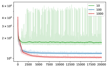
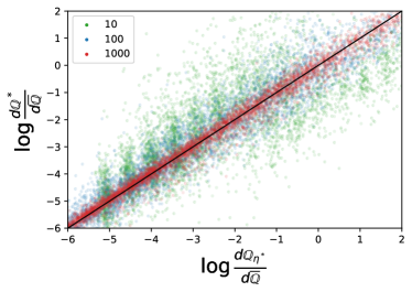
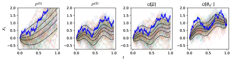
Figure 1: Top: (left) comparison of loss as a function of iteration, and (right) scatter plot of obtain RN derivative versus target, both for various time discretisations. Bottom: evolution under the expert models, average model, and optimal model.

Next, we consider the constraints

$$f(x)={\mathds{1}}_{\{x\in(0.8,1.2)\}}-0.9\,,\quad\text{and}\quad g(t,x)={\mathds{1}}_{\{x<t\}}-0.2\,.$$

These choices of constrains mean that the processes at time $T=1$ should lie with 90% probability within the interval $(0.8,1.2)$, that is ${\mathbb{Q}}(X_{1}\in(0.8,1.2))=0.9$, and that the average time the process spends below a barrier is 0.2, specifically ${\mathbb{E}}^{\mathbb{Q}}[\int_{0}^{1}{\mathds{1}}_{\{X_{u}<t\}}{\rm d}u]\allowbreak=0.2$. In Table 1 we reports the value of the constraints under the two experts models, the average drift model, and the optimal model.

Table 1: Terminal constraints under various measures. ${\mathbb{E}}^{\circ}$ indicates the expectation under the different probability measures indicated in the columns.

	${\mathbb{P}}^{(1)}$	${\mathbb{P}}^{(2)}$	${\mathbb{Q}}[{\bar{\mu}}]$	${\mathbb{Q}}[\theta_{\eta^{*}}]$
${\mathbb{E}}^{\circ}[f(X_{1})]$	$-0.746$	$-0.717$	$-0.626$	$-2.2\times 10^{-3}$
${\mathbb{E}}^{\circ}[\int_{0}^{1}g(u,X_{u})\,{\rm d}u]$	$0.285$	$0.429$	$0.392$	$-5.6\times 10^{-3}$

We observe that the value of the constraints of the average drift model is not the average of the value of the constraints of the experts, this is because ${\mathbb{Q}}[{\bar{\mu}}]$ average the drifts of both experts’ models.

The top two panels of Figure 1 show the corresponding losses during training as well as a scatter plot of the learnt RN derivative for the three different time discretisations. When the number of time steps is small, the discrete approximation of the stochastic integrals cannot capture the optimal measure, generated by $\frac{d{\mathbb{Q}}[\theta_{\eta^{*}}]}{d{\mathbb{Q}}[{\bar{\mu}}]}$, path-by-path. This explains why the scatter plot concentrates more and more along the diagonal as the number of time steps increases. Further, the bottom panel shows sample paths generated by the same Brownian motions for all four models: ${\mathbb{P}}^{(1)}$, ${\mathbb{P}}^{(2)}$, ${\mathbb{Q}}[{\bar{\mu}}]$, and ${\mathbb{Q}}[\theta_{\eta^{*}}]$. We observe that at terminal time, the sample paths are concentrated in the interval (0.8, 1.2) and that the sample paths are shifted upwards to enforce both constraints.

Next we examine how the approach where we learn the drift Algorithm 2 and the approach where we learn the value function compare Algorithm 3 to one another. For this, we consider the same underlying models as above, but with the three constraints

$$f_{1}(x)=(x-1)\,,\qquad f_{2}(x)=(x-1)^{2}-0.05\,,\qquad\text{and}\qquad g_{1}(t,x)={\mathds{1}}_{\left\{x<1-(0.5-t)^{2}\right\}}-0.8\,.$$

The first set of constraints functions are constraints on the mean and variance, in particular ${\mathbb{E}}^{\mathbb{Q}}[X_{1}]=1$ and $\text{var}^{\mathbb{Q}}(X_{1})=0.05$. The running cost constraint is ${\mathbb{E}}^{\mathbb{Q}}[\int_{0}^{1}{\mathds{1}}_{\left\{X_{u}<1-(0.5-t)^{2}\right\}}{\rm d}u]=0.8$.

Figure 2 shows the learnt model in the top panel (both methods produce indistinguishable results), as well as the evolution of the constraint as training progresses. After about 1,000 iterations, both approaches lead to constraints that are well within acceptable errors ($\lesssim 1\times 10^{-3}$) – see the first two panels in the bottom of Figure 2. The right most figure in the bottom panel shows the histogram of the difference between the measure change $\frac{{\rm d}{\mathbb{Q}}[\theta^{*}]}{{\rm d}{\mathbb{Q}}[{\bar{\mu}}]}$ and $\frac{{\rm d}{\mathbb{Q}}[\theta_{\eta^{*}}]}{{\rm d}{\mathbb{Q}}[{\bar{\mu}}]}$ where $\theta^{*}$ is the drift obtained from either learning the drift (Algorithm 2) or learning the value function (Algorithm 3). They have estimated means of $1.1\times 10^{-7}\pm 10^{-3}$ and $6.1\times 10^{-8}\pm 1.1\times 10^{-3}$, respectively. Finally, we estimate the (constrained) KL divergence (2), using Monte Carlo simulations of $10,000$ sample paths, where the optimal $\theta$ stems from Algorithm 2 or Algorithm 3. For Algorithm 2 the estimated (constrained) KL divergence is $1.683\pm 0.005$ and for learning the value function it is $1.660\pm 0.005$. Thus, as expected, learning the value function through elicitability produces an optimal drift that results in a lower KL divergence when compared with learning the drift directly.

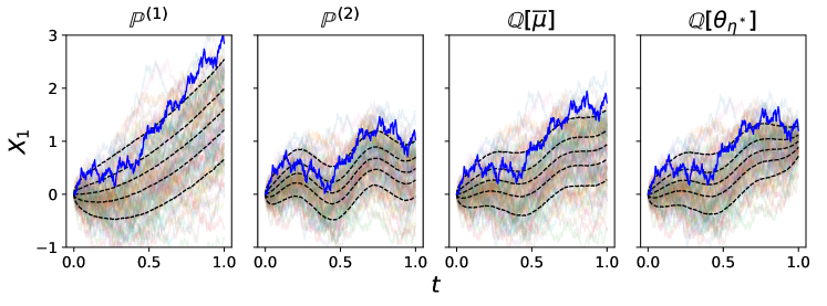
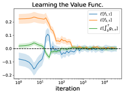
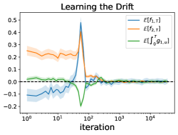
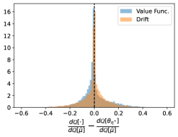
Figure 2: (top) sample paths under the expert models, the average drift model, and the optimal measure. (bottom) The left and middle panels show the evolution of the expectations as the two learning algorithms proceed. The right panel shows the histogram of the difference between the Radon-Nikodym derivative of the learnt model minus $\frac{{\rm d}{\mathbb{Q}}[\theta_{\eta^{*}}]}{{\rm d}{\mathbb{Q}}[{\bar{\mu}}]}$.

4.2 Implied volatility smiles

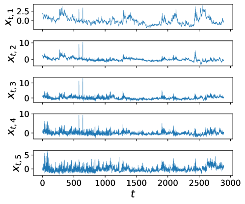
Figure 3: Time series of the (normalised) functional basis coefficients from implied volatility smiles.

In this section we investigate an application to modelling the evolution of implied volatility (IV) smiles. For this we estimate three different models (the expert models) using three distinct time frames and obtain the optimal model with a constraint on the at-the-money skewness. We use daily data for fixed time-to-maturity (TTM) IV smiles from the WRDS database for the assets AMZN at TTM of 60 days over the period July 8, 2010 to December 31, 2021. The data consists of pairs of Delta ($\Delta$) – rather than strike – and IV ($\sigma^{IV}$), that is $(\Delta_{i},\,\sigma^{IV}_{t,i})_{i=1,\dots,17=:I}$, for days $t=1,\ldots,T=2,893$, where $\Delta_{i}=0.1,0.15,\dots,0.9$. We approximate the real-world dynamics of the IV smile using the approach in [7], where the authors consider the entire IV surfaces. Here, we restrict to IV smiles for simplicity. In a first stage, for each time $t$, we project the data onto a functional basis of normalised Legendre polynomials $\{L_{j}(\Delta)\}_{j=0,..,4=:d-1}$ of up to order $4$ using linear regression. That is

$$x_{t}:=\operatorname*{arg\,min}_{a\in{\mathds{R}}^{d}}\sum_{i=1}^{I}\bigg{(}\sum_{j=1}^{d}a_{j}\,L_{j-1}(\Delta_{i})-\sigma_{t,i}^{IV}\bigg{)}^{2}\,,$$

where $x_{t}:=(x_{t,1},\ldots x_{t,d})$. This results in a time-series of coefficients $(\{x_{t,j}\}_{j=1,\dots,d})_{t=1,\dots,T}$, which are shown in Figure 3.

Using the time series $(\{x_{t,j}\}_{j=1,\dots,d})_{t=1,\dots,T}$, we train a neural-SDE model of the form

(19) $${\rm d}X_{t}=\mu(X_{t})\,{\rm d}t+\sigma(X_{t})\,{\rm d}W_{t},$$

with $\mu:{\mathds{R}}^{d}\to{\mathds{R}}^{d}$ and $\sigma:{\mathds{R}}^{d}\to{\rm{S}}^{d}_{++}$, by maximising the likelihood of the observed data subject to a probability integral transform (PIT) penalty – [7] demonstrates that including the PIT penalty significantly decreases model misspecification. By telescoping the likelihood, we have the following loss function

$$-\sum_{t=1}^{T}\Bigg{[}\frac{1}{2\Delta t}\left(\mu(x_{t})\Delta t-\Delta x_{t}\right)^{\intercal}\Sigma^{-1}(x_{t})\left(\mu(x_{t})-\Delta x_{t}\right)+\frac{1}{2}\log\det\big{(}\Sigma(x_{t})\big{)}\Bigg{]}+\zeta\,\sum_{j=1}^{d}PIT_{j},$$

where $\Delta x_{t}:=(\Delta x_{t,1},\ldots,\Delta x_{t,d})$ with $\Delta x_{t,j}:=x_{t+1,j}-x_{t,j}$, $j=1,\ldots,d$, and

$$PIT_{j}:=\int_{0}^{1}\left(\sum_{t=1}^{T}\psi_{h}(u;z_{t,j})-u\right)^{2}{\rm d}u,\quad\text{where}\quad z_{t,j}:=\Phi\left(\frac{\mu_{j}(x_{t})-\Delta x_{t,j}}{\sigma_{j}(x_{t})}\right)\,,$$

and $\zeta$ is a hyper-parameter, $\Phi(\cdot)$ is the standard normal cumulative density function, $\psi_{h}(\cdot)$ is a kernel density with bandwidth $h$ (we use a Gaussian kernel with $h=0.01$), $\mu:=(\mu_{1},\ldots,\mu_{d})$, $\Sigma=\sigma\sigma^{\intercal}$, and $\sigma_{j}=\sqrt{\Sigma_{jj}}$, $j=1,\dots,d$.

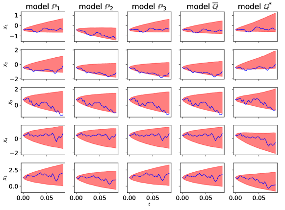
Figure 4: Simulations under the various models. The red bands show the 10% and 90% quantiles at each time point, while the blue line indicates a specific sample path.

To train the neural-SDE we employ two feed forward neural networks with five hidden layers and SiLU activation in all but the output layer for $\mu(x)$ and $\Sigma(x)$ separately. For the output layer, we use a $10\tanh(\cdot)$ activation function to bound the outputs to the range $[-10,10]$ – this improves the speed of convergence of the loss minimisation and also ensures that the resulting dynamics have strong solutions to the associated SDE. For $\Sigma(x)$, we reshape the output of the neural network into a $5$-dimensional lower triangular matrix $U(x)$ and set $\Sigma(x)=U(x)\,(U(x))^{\intercal}+10^{-3}I$, where $I$ is the $5\times 5$ identity matrix, to ensure strict positive definiteness.

To obtain the three expert models, we retrain (19) with a neural SDE model using data restricted to one of $[0,\frac{1}{3}T]$, $(\frac{1}{3}T,\frac{2}{3}T]$, and $(\frac{2}{3}T,T]$, but only retrain the drifts $\mu(x)$. Note that the experts’ models are absolutely continuous with respect to each other, thus they need to share the same volatility $\Sigma(x)$. This results in three distinct (experts) models, whose drift are $\mu^{(1)}(x)$, $\mu^{(2)}(x)$, and $\mu^{(3)}(x)$, and have volatility $\Sigma(x)$.

These three expert models together with the weights $\pi=(0.2,0.2,0.6)$ are then used to approximate the barycentre model subject to the constraint ${\mathbb{E}}^{{\mathbb{Q}}}[\partial_{\Delta}\sigma_{\tau}^{IV}(\Delta)|_{\Delta=\frac{1}{2}}]=0.05$ using the elicitability approach, see Algorithm 3, over a time horizon of $[0,\tau]$ years (with $\tau=\frac{1}{12}$). This constraint imposes that on average, the at-the-money skewness (i.e., at $\Delta=\frac{1}{2})$ of the IV smile at terminal time is equal to $0.05$. Figure 4 displays the sample paths of the 5-dimensional coefficients of the Legendre polynomials under the three experts, the average drift model, and the optimal model. Using simulations of the coefficients under the different models, we then generate under each model sample paths of IV smiles for the time horizon $[0,\tau]$.

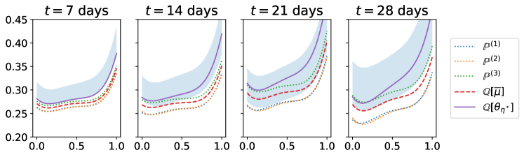
Figure 5: Simulated sample paths of IV smiles for times $t=7,14,21,28$ days under the experts models ${\mathbb{P}}^{(1)},{\mathbb{P}}^{(2)},{\mathbb{P}}^{(3)}$ (dotted), the average drift model ${\mathbb{Q}}[{\bar{\mu}}]$ (dashed), and ${\mathbb{Q}}[\theta_{\eta^{*}}]$ (solid). Shaded blue area are the 10% to 90% bands for the simulated IV smiles under ${\mathbb{Q}}[\theta_{\eta^{*}}]$. The weights for the experts are $\pi=(0.2,0.2,0.6)$.

Figure 5 show a sample path of IV smiles from each expert, the model ${\mathbb{Q}}[{\bar{\mu}}]$, and the learnt constrained barycentre model ${\mathbb{Q}}[\theta_{\eta^{*}}]$, for four different times $t\in[0,28]$ days. The plots also display the $10\%$ to $90\%$ band of for $10,000$ sample paths from the ${\mathbb{Q}}[\theta_{\eta^{*}}]$ model. We observe that for later days, the bands increase and the models deviate from one another. Moreover, the displayed sample IV smile under ${\mathbb{Q}}[\theta_{\eta^{*}}]$ becomes steeper at $\Delta=\frac{1}{2}$ to meet the constraint.

5 Conclusions

We present an approach to combine expert models, based on minimisation of the weighted KL divergence between the experts’ models and a candidate model, that incorporates the agent’s beliefs in the form of expectation constraints. The proposed methodology may be suitable to combine models in a multitude of settings in mathematical finance ranging from climate finance, to volatility modelling, and high-frequency trading. Moreover the resulting optimal model can be reinterpreted as a generative model for, e.g., a dynamic risk-aware reinforcement learning approach to mitigating risks and optimising portfolio allocation [8, 16] or generating climate scenarios that feed into risk management for carbon planning [14].

References

• [1] J. M. Altschuler and E. Boix-Adsera, Wasserstein barycenters are NP-hard to compute, SIAM Journal on Mathematics of Data Science, 4 (2022), pp. 179–203.
• [2] J. Backhoff-Veraguas, S. Källblad, and B. A. Robinson, Adapted Wasserstein distance between the laws of SDEs, arXiv preprint arXiv:2209.03243, (2022).
• [3] D. J. Berndt and J. Clifford, Using dynamic time warping to find patterns in time series, in Proceedings of the 3rd international conference on knowledge discovery and data mining, 1994, pp. 359–370.
• [4] J. Bion-Nadal and D. Talay, On a Wasserstein-type distance between solutions to stochastic differential equations, The Annals of Applied Probability, 29 (2019), pp. 1609–1639.
• [5] L. Breiman, Bagging predictors, Machine Learning, 24 (1996), pp. 123–140.
• [6] L. Breiman, Prediction games and arcing algorithms, Neural Computation, 11 (1999), pp. 1493–1517.
• [7] V. Choudhary, S. Jaimungal, and M. Bergeron, Funvol: A multi-asset implied volatility market simulator using functional principal components and neural SDEs, arXiv preprint arXiv:2303.00859, (2023).
• [8] A. Coache, S. Jaimungal, and Á. Cartea, Conditionally elicitable dynamic risk measures for deep reinforcement learning, SIAM Journal on Financial Mathematics, 14 (2023), pp. 1249–1289.
• [9] I. Csiszár, I-divergence geometry of probability distributions and minimization problems, The Annals of Probability, (1975), pp. 146–158.
• [10] P. D’Urso, L. De Giovanni, and R. Massari, Trimmed fuzzy clustering of financial time series based on dynamic time warping, Annals of operations research, 299 (2021), pp. 1379–1395.
• [11] T. Fissler and S. M. Pesenti, Sensitivity measures based on scoring functions, European Journal of Operational Research, 307 (2023), pp. 1408–1423.
• [12] T. Gneiting, Making and evaluating point forecasts, Journal of the American Statistical Association, 106 (2011), pp. 746–762.
• [13] L. K. Hansen and P. Salamon, Neural network ensembles, IEEE transactions on pattern analysis and machine intelligence, 12 (1990), pp. 993–1001.
• [14] M. Hellmich and R. Kiesel, Carbon Finance: A Risk Management View, World Scientific, 2021.
• [15] S. Jaimungal, S. M. Pesenti, and L. Sánchez-Betancourt, Minimal Kullback–Leibler divergence for constrained Lévy–Itô processes, SIAM Journal on Control and Optimization, 62 (2024), pp. 982–1005.
• [16] S. Jaimungal, S. M. Pesenti, Y. F. Saporito, and R. S. Targino, Risk budgeting allocation for dynamic risk measures, arXiv preprint arXiv:2305.11319, (2023).
• [17] B.-H. Juang, On the hidden Markov model and dynamic time warping for speech recognition—a unified view, AT&T Bell Laboratories Technical Journal, 63 (1984), pp. 1213–1243.
• [18] E. Kroell, S. M. Pesenti, and S. Jaimungal, Stressing dynamic loss models, Insurance: Mathematics and Economics, 114 (2024), pp. 56–78.
• [19] H. Skutkova, M. Vitek, P. Babula, R. Kizek, and I. Provaznik, Classification of genomic signals using dynamic time warping, BMC bioinformatics, 14 (2013), pp. 1–7.
• [20] D. West, S. Dellana, and J. Qian, Neural network ensemble strategies for financial decision applications, Computers & operations research, 32 (2005), pp. 2543–2559.
• [21] L. Yu, S. Wang, and K. K. Lai, Forecasting crude oil price with an emd-based neural network ensemble learning paradigm, Energy economics, 30 (2008), pp. 2623–2635.