The mechanism of electrical conduction in glassy semiconductors
Abstract
We argue that the dominant charge carrier in glassy semiconducting alloys is a compound particle in the form of an electron or hole bound to an intimate pair of topological lattice defects; the particle is similar to the polaron solution of the Su-Schrieffer-Heeger Hamiltonian. The spatial component of the density of states for these special polarons is determined by the length scale of spatial modulation of electronegativity caused by a separate set of standalone topological defects. The latter length scale is fixed by the cooperativity size for structural relaxation; the size is largely independent of temperature in the glass but above melting, it decreases with temperature. Thus we predict that the temperature dependence of the electrical conductivity should exhibit a jump in the slope near the glass transition; the size of the jump is predicted to increase with the fragility of the melt. The predicted values of the jump and of the conductivity itself are consistent with experiment.
The microscopic mechanism of electrical conduction in amorphous semiconductors is a long-standing question of condensed matter physics. In Mott’s picture [1, 2], electrical current in amorphous semiconductors is carried through relatively extended, wavepacket-like electronic excitations. The lattice remains largely a spectator of electronic motions, vibrations being a perturbation as in Migdal’s theorem [3]. Owing to the disorder, the electronic bands are not collections of extended Bloch states, but, instead, are mobility bands composed of orbitals whose extent only needs to be greater than the mean free path of the electronic quasiparticle. Emin [4, 5] argued that when the electron-lattice coupling is sufficiently strong, the current is carried, instead, by small polarons [6]. The small polaron is a compound, emergent entity in the form of a self-trapped electron or hole that occupies an impurity-like bound state. The bound state is due to a local deformation of the lattice stabilized by the trapped charge itself; its formation is subject to an activation barrier [6]. Mott’s and Emin’s scenarios each predict an Arrhenius temperature dependence of the conductivity, the activation energy tied to the optical gap. Both descriptions are continuum, the microscopic length scale provided by the spatial concentration of the frontier orbitals, irrespective of the material’s structure.
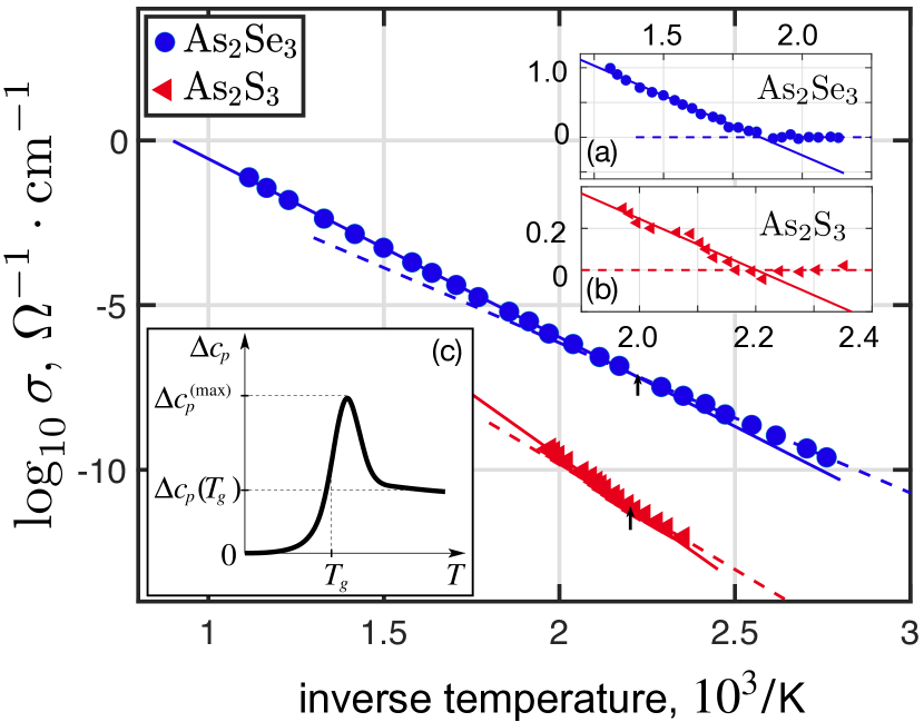
The optical gap [7, 8, 9] and the structure [10, 11] of a glassy melt both vary continuously with temperature across the glass transition. The treatments in Refs. [2, 4] thus imply the electrical conductivity should depend smoothly on temperature near the glass transition temperature . Contrary to this expectation, the measured temperature dependence of the electrical conductivity exhibits a distinct jump in the slope at [12], see Fig. 1.
To rationalize this apparent, puzzling connection between electronic and structural properties of glassy semiconductors, here we put forth an expressly non-continuum picture. It derives from relatively recent findings that glassy melts and frozen glasses alike exhibit organization on two length scales. The smaller of these length scales, often called the bead size [16, 17], corresponds with the first sharp diffraction peak [18, 19] and is only marginally greater than the atom spacing. This length is static and reflects a symmetry breaking at the level of the first coordination shell [10] caused by the anisotropy in bonding intrinsic to electron-rich centers [20, 21, 22]. The pertinent particle spacing in the symmetry-lowered structure can be thought of as the size of a rigid molecular unit that is perturbed only weakly during structural relaxation [10, 23]. The greater length, often called the cooperativity size [24], is the volumetric size of the smallest region than can reconfigure in the glassy material [25, 11, 26]. In a frozen glass, nm, cm-3 [27], approximately independent of temperature [11]. Upon melting, the length begins to decrease with temperature and drops down to or so, in magnitude, by the dynamical crossover, beyond which the system becomes a uniform liquid [17, 28, 29]. This microscopic picture has quantitatively explained dozens of disparate phenomena in glassy melts and frozen glasses, see reviews [30, 31, 32, 33]. Though of dynamical origin [30, 34, 35], the length has a static aspect in that it provides the characteristic length scale for the spatial variation of the excess strain of the glassy matrix [26, 31].
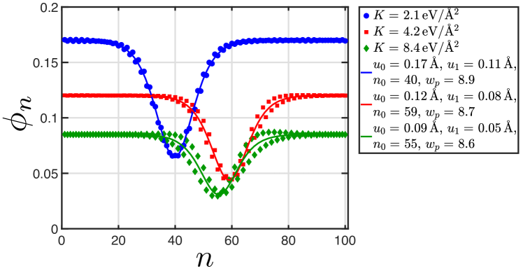
We have argued that in glassy semiconductors that charge-density-wave (CDW) solids, such strained regions host midgap electronic states [36, 37, 38]. These special midgap states are similar to the topological midgap states arising when the two alternative dimerization patterns of a trans-polyacetylene chain are brought into contact [36, 39]. This picture provides a unified, quantitative explanation for the puzzling light-induced midgap absorption and electron paramagnetic resonance signal [40, 41, 42], anomalous fluorescence [42, 43, 44], and difficulty in doping glassy semiconductors [45, 46]. We illustrate here the emergence of these special midgap states by considering a Peierls-distorted chain of electron-hosting sites at half-filling, at the level of the Su-Schrieffer-Heeger (SSH) Hamiltonian [39]. The spatial profile of the staggered displacement of the sites, in the ground state of an odd-numbered, closed chain is shown with circles in Fig. 2. There is a topologically stable defect in the dimerization pattern—owing to the odd number of sites—that cannot be removed by elastic deformation. The conduction and valence edges, respectively, of the insulating gap effectively cross at the defect, thus leading to the appearance of a midgap electronic state there [47, 39, 38]. Inset (a) of Fig. 2 shows a neutral midgap state with spin ; it can be thought of as a solid-state analog of a free radical.
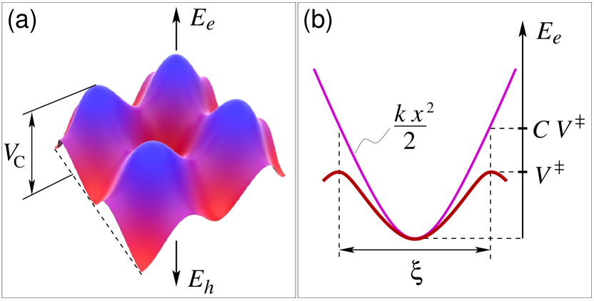
A topological midgap state in a glassy semiconductor is typically charged negatively or positively [36, 37, 38], which would correspond to the singly-occupied state in Fig. 2, inset (a), becoming instead either filled or empty, respectively. The so charged defects thus comprise a disordered checkerboard pattern of excess negative and positive charges, the corresponding length scale being the cooperativity length itself. The pattern is tied to the structure and can change only if the melt flows or ages; both of the latter processes are activated and, typically, slow [30, 31]. The aperiodic checkerboard charge pattern is a source of an electrostatic potential, see Fig. 3(a), that will act on itinerant charges.
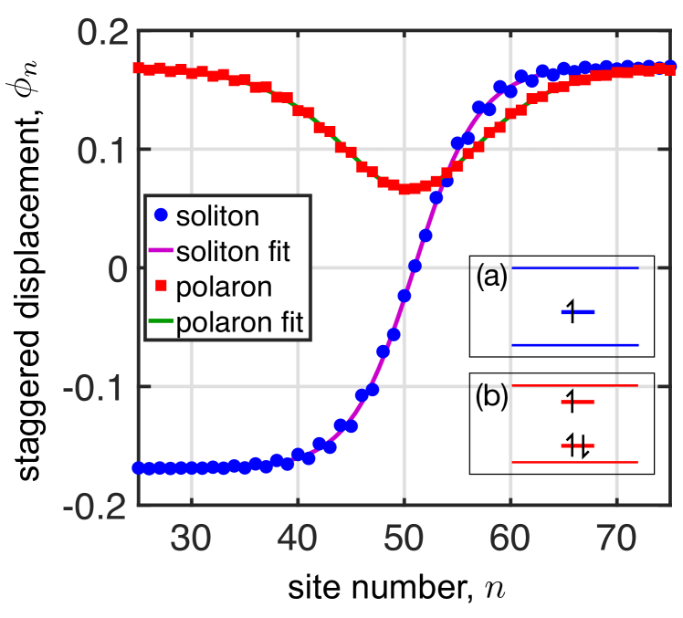
To determine the detailed nature of itinerant charges in glassy CDW solids, we note that already their periodic counterparts can house intimate pairs of topological defects bound to a polaron [48, 49, 39]. We illustrate such an (electron) polaron configuration in Fig. 2, at the SSH level, using an even-numbered closed chain at half-filling and an added electron. In the extreme limit of a chain of weakly interacting dimers, this special polaron can be thought of as an electron placed in the anti-bonding orbital on an individual dimer, inset (b) of Fig. 2. At the same time, a destabilization of the filled orbital takes place. The bonding—anti-bonding orbital pair corresponds to two mutually-hybridized midgap states centered on, respectively, an over-coordinated and under-coordinated site [39]. The hole-polaron case is analogous and would correspond to an empty antibonding orbital and half-filled bonding orbital in Fig. 2, inset (b).
An extended carrier turns into the topological polaron via a downhill, barrierless process that results in a relatively extended deformation pattern, shown with squares in Fig. 2. Polaron-like configurations analogous to that in Fig. 2 have been obtained at an ab initio level in 3D samples of disordered chalcogenide alloys [38]. The corresponding orbitals are part of the Urbach-Lifshitz tail of the localized states [38, 9] and can contain one or more quasi-linear fragments, each of which is similar to the topological polaron in conjugated polymers [48, 49, 39].
The electrical conductivity is a sum of the contributions from the electron () and hole () polarons, respectively:
| (1) |
where is the density of thermally available polaron states, the effective charge, and the mobility, respectively, of carrier at energy .
The polaron must be centered on a covalent bond, per Fig. 2, inset (b). Each pnictogen typically forms three such bonds, chalcogen two [50]. The bonding is locally distorted-octahedral, where the number of covalent bonds is approximately a half of the total number of the inter-atomic contacts, the rest being weaker, closed-shell interactions [50, 10]. At the same time, the covalent bonds must be associated with rigid molecular units; thus their volumetric volume should be equated with the bead size ; generically Å in chalcogenides Ref. [36]. Pretend for a moment that the underlying lattice and the potential due to the built-in charged topological defects, Fig. 3(a), are both strictly periodic and have the same point-group symmetry. The lowering of the translational symmetry, due to the potential, would result in a reduction of the Brillouin zone, relative to the potential-free case, by a factor of along each spatial dimension. The new, smaller zone would then contain distinct polaron bands per each band in the original, large zone.
The potential in Fig. 3(a) is aperiodic but, more importantly, it exhibits enough variation, eV, for the polaron (mobility) bands to become so narrow as to break up into distinct sets of vibrational levels within respective wells. This is similar to how core electronic orbitals in a solid do not form bands but, instead, remain localized. Indeed, first we note the potential around an individual charged defect is parabolic in the vicinity of its respective minimum, denote the corresponding spring constant with . Thus the vibrational quantum number for motion in one spatial direction is limited from above, so that , where is the altitude of the lowest saddle point relative to the bottom of the well, , the soliton’s mass, and is a numerical constant. The latter constant specifies, by construction, how much the parabolic approximation exceeds the actual potential near the saddle point: , see Fig. 3(b). The total number of the vibrational states for three-dimensional motion is approximately . To estimate the value of above which every polaron band must cross classically forbidden regions, we require that the number of bands be less than . The mass of the soliton is significantly lower than the atomic mass , because a displacement of the soliton over a lattice spacing implies a much smaller displacement, or so, for an actual atom [24, 39]: . The length , often called the Lindemann length [51], is the displacement at the mechanical stability edge of a solid. We set , for concreteness, to obtain:
| (2) |
Using and , where is the electron mass, one obtains eV, which is much less than . As a consequence, the tunneling matrix element for inter-well tunneling is astronomically small: , where we used the standard WKB expression for the under-barrier wavefunction and Eq. 2.
The localization of the polarons means that the translational degrees of freedom of the itinerant charge have been effectively converted into vibrations of the polaron around an individual charged center. The expectation value of the polaron’s vibrational coordinate is at the center of the respective well of the potential from Fig. 3(a), be the vibration in the ground or any of the excited states. As a result, the location of the polaron can be only determined up to the spacing between nearby centers, i.e., the length itself. Thus the spatial component of the density of states for charge carriers must be equal to , not the usually postulated density of valence electrons/holes.
At the same time, because the tunneling between distinct minima is negligible, the polaron must move via thermally-activated, adiabatic transitions [52] between nearby minima on the potential surface from Fig. 3(a). An individual jump is thus of length . At the transition state, the electron/hole is delocalized at least over a distance and is best thought of as belonging to the pertinent mobility band. The activation barrier for polaron’s hopping between pairs of distinct attractive wells is then determined by the distance from the polaron level ( for electrons, for holes) to the edge of the appropriate mobility band ( conduction, valence band). Thus we obtain for the electron (hole) polaron hopping rate: (), and for the (long-time) diffusivity . To determine the prefactor we note that the bonds must return to their equilibrium lengths when the polaron delocalizes. Thus the reaction coordinate near the transition state is essentially the vibration of the covalent bond where the polaron is centered at the moment, denote the respective frequency with . Away from the transition state, the reaction coordinate increasingly hybridizes with other vibrational modes, implying a barrier-crossing event will have likely succeeded after a single vibration of the reaction coordinate. Consequently the prefactor can be well approximated by its value near critical damping, [52]. The energy dependence of the equilibrium density of states for electrons, at the energies in question, is given by the Boltzmann factors , being the chemical potential. The overall activation rate determining the conductivity in Eq. 1 becomes the Arrhenius factor for electrons and for holes. Thus Eq. 1 yields:
| (3) |
where only the dominant term inside the square brackets should be used.
We discuss implications of Eq. 3 for the -dependence of for an experimental protocol [14], in which electrodes are deposited on a glass sample, after which the conductivity is measured for a set of temperatures , . According to the random first-order transition (RFOT) theory [31, 30], the cooperativity size will remain near stationary in the glass but will be decreasing with temperature above melting, a good approximation provided by the expression [26] . Here is the configurational entropy per unit volume and is the bulk modulus. As a result, the -derivative of the length and, hence, of the conductivity should exhibit a discontinuity at the glass transition. The discontinuity is somewhat smeared because the relaxation times in the glass are distributed [34, 53]. Thus we obtain a simple relation for and for . This yields that the apparent activation energy should exhibit a discontinuity at the glass transition:
| (4) |
Here is the peak value of the excess heat capacity of the liquid relative to the frozen glass, as determined using the same protocol as that for the measurements. During melting, undergoes a (smeared) jump from zero to a positive value and, then, gradually declines with temperature. The latter gradual decline is often preceded by a sharp peak, whose height is the greater, the more slowly the glass had been prepared [54], see illustration in Fig. 1, inset (c). The overshoot, if any, comes about because glasses are the more stable the more slowly they are prepared [11, 31]. Consequently, we expect that the jump in the apparent activation energy will exhibit a range of values depending on the detailed preparation protocol. By construction,
| (5) |
The configurational entropy at the glass transition can be well approximated according to [27, 17], where is the melting entropy of the corresponding crystal. The quantity in the melt is generically around unity in chalcogenides [55]; we set for concreteness, see also SM.
| material | (exp), eV | (th), eV |
|---|---|---|
| As2Se3 | ||
| As2S3 | 0.093 |
The range of predicted values of for the selenide, see Table 1, corresponds to the range of heights of the peaks reported in Ref [54]. The sulfide calorimetry data we found [56] do not exhibit a peak; the one value we provide for the sulfide should be regarded as a lower bound. We see the present predictions are consistent with experiment, while suggesting the samples had been aged.
When the peak is absent – corresponding to the equality in Eq. 5 – one may connect to the conventional fragility coefficient , where is the -relaxation time and the corresponding free energy barrier. Since [26], one obtains:
| (6) |
Eq. 5 then implies:
| (7) |
is readily measured. The dynamical range of the glassy melt, , is certainly less than but, most likely, no less than . Thus the quantity multiplying in the equation above is greater than or so. For known substances [31], which implies the jump should be distributed, among different substances, within the range or so. Other relations connecting to material properties can be written, see SM.
The optical gap itself exhibits a temperature dependence [9], which is approximately linear around . This will contribute to the apparent pre-exponential factor in Eq. 3. We estimate the overall apparent prefactor, see SM, to be around S/cm, consistent with Fig. 1. The prefactor in Emin’s scenario is somewhat greater but is comparable to the present prediction. Emin’s scenario also predicts a non-vanishing since a melt expands more readily with temperature than the respective glass, but this volumetric effect is two orders of magnitude weaker than the prediction in Eq. 4, see SM.
The present picture applies to glassy materials that host charge-density waves [36, 10]. All known glassy semiconductors appear to fit into this category, whereby the bond order varies within unity while the magnitude of electronegativity variation is modest. Disordered semiconductors that are made by deposition—or using other non-equilibrium methods—may or may not house a CDW. For instance, amorphous silicon films exhibit (distorted) tetrahedral bonding whose saturation is spatially uniform, and thus lack CDWs. At the same time silicon does not vitrify readily in the first place.
Acknowledgments: V. L. thanks David Emin for insightful conversations. We gratefully acknowledge the support by the NSF Grants CHE-1465125 and CHE-1956389, the Welch Foundation Grant E-1765, and a grant from the Texas Center for Superconductivity at the University of Houston.
References
- Mott and Davis [1979] N. F. Mott and E. A. Davis, Electronic Processes in Non-crystalline Materials (Clarendon Press, Oxford, 1979).
- Mott [1993] N. F. Mott, Conduction in Non-crystalline Materials (Clarendon Press, Oxford, 1993).
- Migdal [1958] A. Migdal, Sov. Phys. JETP 7, 996 (1958).
- Emin [1983a] D. Emin, Comments Solid State Phys. 11, 35 (1983a).
- Emin [1983b] D. Emin, Comments Solid State Phys. 11, 59 (1983b).
- Emin and Holstein [1976] D. Emin and T. Holstein, Phys. Rev. Lett. 36, 323 (1976).
- Arai et al. [1975] T. Arai, S. Komiya, and K. Kudo, JNC 18, 295 (1975).
- Hosokawa et al. [1991] S. Hosokawa, Y. Sakaguchi, H. Hiasa, and K. Tamura, J. Phys. Cond. Mat. 3, 6673 (1991).
- Lubchenko and Kurnosov [2019] V. Lubchenko and A. Kurnosov, J. Chem. Phys. 150, 244502 (2019).
- Lukyanov and Lubchenko [2017] A. Lukyanov and V. Lubchenko, J. Chem. Phys. 147, 114505 (2017).
- Lubchenko and Wolynes [2004] V. Lubchenko and P. G. Wolynes, J. Chem. Phys. 121, 2852 (2004).
- Seager and Quinn [1975] C. H. Seager and R. K. Quinn, J. Non-Cryst. Sol. 17, 386 (1975).
- Davey and Baker [1983] T. C. Davey and E. H. Baker, J. Mater. Sci. 18, 717 (1983).
- Bobb et al. [1975] L. C. Bobb, H. H. Byer, and K. Kramer, Electrical properties of As2S3 glass, techreport (Pitman-Dunn Laboratory, U.S. ARMY ARMAMENT COMMAND, FRANKFORD ARSENAL, PHILADELPHIA, PENNSYLVANIA 19137, 1975) https://apps.dtic.mil/sti/citations/tr/ADA020552.
- Kolomiets [1964] B. T. Kolomiets, physica status solidi (b) 7, 713 (1964).
- Xia and Wolynes [2000] X. Xia and P. G. Wolynes, Proc. Natl. Acad. Sci. U. S. A. 97, 2990 (2000).
- Lubchenko and Wolynes [2003] V. Lubchenko and P. G. Wolynes, J. Chem. Phys. 119, 9088 (2003).
- Salmon [1994] P. Salmon, Proc. R. Soc. Lond. A 445, 351 (1994).
- Elliott [1991] S. R. Elliott, Nature 354, 445 (1991).
- Papoian and Hoffmann [2000] G. A. Papoian and R. Hoffmann, Angew. Chem. Int. Ed. 39, 2408 (2000).
- Golden et al. [2017] J. C. Golden, V. Ho, and V. Lubchenko, J. Chem. Phys. 146, 174502 (2017).
- Albright et al. [2013] T. A. Albright, J. K. Burdett, and M.-H. Whangbo, Orbital Interactions in Chemistry (Wiley, Hoboken, NJ, 2013).
- Bevzenko and Lubchenko [2009] D. Bevzenko and V. Lubchenko, J. Phys. Chem. B 113, 16337 (2009).
- Lubchenko and Wolynes [2001] V. Lubchenko and P. G. Wolynes, Phys. Rev. Lett. 87, 195901 (2001).
- Kirkpatrick et al. [1989] T. R. Kirkpatrick, D. Thirumalai, and P. G. Wolynes, Phys. Rev. A 40, 1045 (1989).
- Lubchenko and Rabochiy [2014] V. Lubchenko and P. Rabochiy, J. Phys. Chem. B 118, 13744 (2014).
- Rabochiy et al. [2013] P. Rabochiy, P. G. Wolynes, and V. Lubchenko, J. Phys. Chem. B 117, 15204 (2013).
- Stevenson et al. [2006] J. D. Stevenson, J. Schmalian, and P. G. Wolynes, Nature Physics 2, 268 (2006).
- Rabochiy and Lubchenko [2012] P. Rabochiy and V. Lubchenko, J. Chem. Phys. 136, 084504 (2012).
- Lubchenko and Wolynes [2007a] V. Lubchenko and P. G. Wolynes, Annu. Rev. Phys. Chem. 58, 235 (2007a).
- Lubchenko [2015] V. Lubchenko, Adv. Phys. 64, 283 (2015).
- Lubchenko and Wolynes [2007b] V. Lubchenko and P. G. Wolynes, Adv. Chem. Phys. 136, 95 (2007b), https://arxiv.org/abs/cond-mat/0506708.
- Lubchenko [2018] V. Lubchenko, Advances in Physics: X 3, 1510296 (2018).
- Xia and Wolynes [2001] X. Xia and P. G. Wolynes, Phys. Rev. Lett. 86, 5526 (2001).
- Lubchenko and Wolynes [2020] V. Lubchenko and P. G. Wolynes, J. Phys. Chem. B 124, 8434 (2020).
- Zhugayevych and Lubchenko [2010a] A. Zhugayevych and V. Lubchenko, J. Chem. Phys. 132, 044508 (2010a).
- Zhugayevych and Lubchenko [2010b] A. Zhugayevych and V. Lubchenko, J. Chem. Phys. 133, 234504 (2010b).
- Lukyanov et al. [2018] A. Lukyanov, J. C. Golden, and V. Lubchenko, J. Phys. Chem. B 122, 8082 (2018).
- Heeger et al. [1988] A. J. Heeger, S. Kivelson, J. R. Schrieffer, and W. P. Su, Rev. Mod. Phys. 60, 781 (1988).
- Biegelsen and Street [1980] D. K. Biegelsen and R. A. Street, Phys. Rev. Lett. 44, 803 (1980).
- Hautala et al. [1988] J. Hautala, W. D. Ohlsen, and P. C. Taylor, Phys. Rev. B 38, 11048 (1988).
- Tada and Ninomiya [1989a] T. Tada and T. Ninomiya, Sol. St. Comm. 71, 247 (1989a).
- Tada and Ninomiya [1989b] T. Tada and T. Ninomiya, J. Non-Cryst. Sol. 114, 88 (1989b).
- Tada and Ninomiya [1989c] T. Tada and T. Ninomiya, J. Non-Cryst. Sol. 137&138, 997 (1989c).
- Anderson [1975] P. W. Anderson, Phys. Rev. Lett. 34, 953 (1975).
- Kolomiets [1981] B. T. Kolomiets, J. Phys. (Paris) C4 42, 887 (1981).
- Jackiw and Rebbi [1976] R. Jackiw and C. Rebbi, Phys. Rev. D 13, 3398 (1976).
- Su and Schrieffer [1980] W. P. Su and J. R. Schrieffer, Proc. Natl. Acad. Sci. U. S. A. 77, 5626 (1980).
- Brazovskii and Kirova [1981] S. Brazovskii and N. Kirova, JETP Lett. 33, 4 (1981).
- Zhugayevych and Lubchenko [2010c] A. Zhugayevych and V. Lubchenko, J. Chem. Phys. 133, 234503 (2010c).
- Lubchenko [2006] V. Lubchenko, J. Phys. Chem. B 110, 18779 (2006).
- Frauenfelder and Wolynes [1985] H. Frauenfelder and P. G. Wolynes, Science 229, 337 (1985).
- Lubchenko [2007] V. Lubchenko, J. Chem. Phys. 126, 174503 (2007).
- Eastel et al. [1977] A. J. Eastel, J. A. Wilder, R. K. Mohr, and C. T. Moynihan, J. Amer. Ceramic Soc. 60, 134 (1977).
- Gadaud and Pautrot [2003] P. Gadaud and S. Pautrot, J. Non-Cryst. Sol. 316, 146 (2003).
- Wagner et al. [1998] T. Wagner, S. O. Kasap, M. Vlcek, A. Sklenár, and A. Stronski, J. Mater. Sci. 33, 5581 (1998).
Supplementary Material
I The topological midgap state and polaron solution of the Su-Schrieffer-Heeger Hamiltonian
We describe the topological defects and the accompanying electronic states that arise in Peierls-dimerized chains using the Su-Schrieffer-Heeger Hamiltonian [1]:
| (S1) |
Here () creates (annihilates) an electron with spin at site . The lattice component of the full energy describes, at a quadratic level, inter-site interactions as they would be in the absence of frontier electrons:
| (S2) |
where is the spring constant, is the atomic mass, and the displacements of the site off the locations they would have in a chain with undeformed springs.
We follow SSH by adopting the following parametrization of the hopping matrix element as a function of the inter-site separation:
| (S3) |
which is a linear approximation for the actual, approximately exponential dependence of inter-site matrix elements.
The on-site energies are introduced, as in Refs. [2, 3], to model a spatial distribution of the electronegativity. For concreteness we adopt a perfectly alternating pattern of electronegativity variation along the chain:
| (S4) |
This is the case considered and solved by Rice and Mele [2], who showed that the system will become Peierls-stable when the electronegativity variation exceeds a certain threshold value. In the latter case, the chain does not spontaneously form a charge-density wave (CDW) but, instead, represents an ionic insulator. Thus we adopt here a sufficiently small value of such that the (doubly-degenerate) ground state of our chain, at half-filling, is a perfectly Peierls-dimerized chain. Denote the ground state value of the staggered displacement
| (S5) |
with . (The latter quantity is doubly degenerate.) Denote the values of the larger and smaller overlap integrals with and , respectively. This system does host a charge-density wave, whose magnitude scales approximately linearly with the hopping-element differential .
We next choose concrete values for the parameters , , and that are roughly consistent with mechanical and electronic properties of the chalcogenides of interest, such as arsenic selenide or sulphide. The optical gap is about 1.8 eV for As2Se3, eV for As2S3. For concreteness, we set the insulating gap in the ground state of our dimerized chain at 2 eV, at . This provides a constraint for the hopping matrix element differential: . An additional constraint on the parameters can be obtained by noting that the zone width in the SSH Hamiltonian, at , is approximately equal to [1]:
| (S6) |
while the width of the valence zone is calculated to be around 6 eV [4]. This, then, imposes bounds on the choice of the parameter since the spring constant should be in the range eVÅ [5]. In what follows, we adopt values eV and eV.
Excitations in the SSH Hamiltonian can be quite complicated because they mutually couple the electronic and vibrational motions, even though there is no interaction within the respective individual sets of motions. To simplify reasoning, it is often useful to think of a dimerized chain in an ultra-local limit of a set of weakly interacting dimers [4], whereby . As a concrete chemical implementation of this limit, imagine an even-numbered chain of hydrogen atoms. It is obvious that for its ground state, such a chain will break up into a set of H2 dimers, so that the bonding within each dimer is covalent, while nearest-neighbor dimers are coupled but weakly, through a closed-shell interaction. In this extreme limit and , it is obvious that a chain containing an odd number of atoms, in its ground state, will have precisely one excess weak or strong bond. Molecular realizations of the latter arrangement, as pertinent to chalcogenide alloys, can be found in Refs. [6, 7, 4]. Such coordination defects can only be removed by changing the number of sites and, therefore, are topologically stable against vibrations. At the defect, the staggered displacement will exhibit a discrete sign reversal. The cases of an excess weak and strong bond can be thought of as an extra single site or an extra trimer, respectively [7]. In either case, there will appear an edge-like, non-bonding orbital located inside the forbidden gap [4].
When the disparity between the hopping elements and is not very large, the defect and the accompanying midgap state will persist, but the aforementioned discrete sign change will be replaced by a milder, sigmodal curve. In other words, the deviation from the perfect coordination pattern, as well as the accompanying excess strain, are now distributed over a relatively extended region. At the center of the strained region, the bonds will be intermediate, length- and strength-wise, between the weak and strong bond, respectively, of a dimerized chain [6]. The width of the kink scales roughly inversely proportionally with the band gap [1, 3]. It is common to fit the sigmodal dependence using the following functional form:
| (S7) |
This form becomes exact in the continuum limit [8, 1]. The latter limit also drives home the solitonic nature of the coordination defect. The parameter can be thought of as the half-width of the soliton.
For a chain at half-filling, the midgap state will be singly occupied. The resulting energy cost is about for a long chain; it tends asymptotically to in the continuous limit [8]. We show a soliton in its vibrational ground state, at , for a closed chain of 101 sites in Fig. S1.
The topological solitons represent a family of gapped excitations of the chain. While we generated the soliton solution above by employing an odd-numbered chain—which drove home the soliton’s topological nature—such solitons can be generated in extended chains irrespective of the parity of the total chain length. Indeed, following activation, a pair of defects can spontaneously emerge in a perfectly dimerized chain, one defect corresponding to an undercoordinated center, the other to an overcoordinated center [1, 3]. Imagine that the so emerged two defects fail to mutually annihilate but, instead, separate in space. An individual soliton or anti-soliton should each be considered as a standalone excitation, the same way we consider electrons and holes as standalone excitations. A chain housing a standalone soliton will equilibrate vibrationally yet no restoring force from the chain will appear that attempts to remove the soliton; the latter can be removed only via annihilation with a separate solition of opposite polarity, as already alluded to. In addition, the soliton can travel unimpeded along the chain [1].
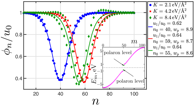
An alternative set of intrinsically gapped excitations for a vibrationally equilibrated chain come about when an electron/hole is added to the conduction/valence band. This type of excited state represents a polaron. It is common for electronically excited states to interact with the lattice and, in particular, with optical phonons [9]. Such interactions serve to stabilize charge-separated states, resulting in a Stokes shift in photoemission, among other things. Similarly, the total energy of a polaron in a Peierls-distorted chain will be lowered somewhat relative to the width of the insulating gap, following vibrational relaxation of the chain [10, 11, 1]. In fact, the corresponding vibration should be classified largely as an optical vibrational mode: In the presence of a polaron, the stronger bond housing the polaron will elongate, as mentioned in the main text. This is an optical mode because it involves displacement within a unit cell of the dimerized chain. Alternatively, this displacement can be thought of an intimate soliton—anti-soliton pair because it attempts to create, next to each other, two nearest-neighbor short bonds, on the one hand, and two nearest-neighbor long bonds, on the other hand. This suggests that one may fit the resulting spatial profile of the staggered displacement using the spatial derivative of the solitonic profile from Eq. S7, viz.:
| (S8) |
We note that at the SSH level, the energy of the polaron level, relative to the middle of the gap, depends on the parameters through the gap width alone, at [12, 11, 13]:
| (S9) |
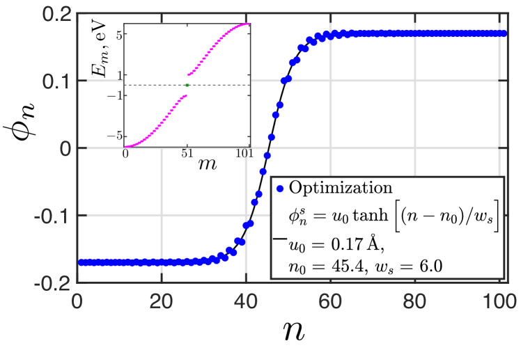
Here we illustrate the polaron solution, at . We have optimized a chain of length filled with electrons. The result is shown in Fig. S2. The splitting of polaron levels off the edges of the electronic bands is eV for the gap eV, in agreement with Eq. S9. We have observed that the polaron width is independent of the spring constant as long as the electron-phonon coupling is adjusted so as to maintain the gap fixed.
In the main text, we illustrate the soliton and polaron solutions at a non-vanishing value of eV, as would be appropriate for chalcogenides. The rest of the parameters are as follows: eV, eV/Å, and eV/Å. Both solutions are qualitatively and quantitatively similar to solutions obtained at , consistent with the notion that these excitations come about owing to the charge-density wave, while the non-vanishing electronegativity variation is a perturbation.
II Estimates
II.1 Experimental data and fits
First we provide the result of our fits of the measured conductivity data. We fit the vs. curve for each substance using a set of two straight lines, one line pertaining to , the other to . The corresponding negative slopes are denoted with and , respectively. The error of the slopes is evaluated within the -confidence interval.
| (S10) |
| Material | , eV | , eV | , eV |
|---|---|---|---|
| As2Se3 [14] | |||
| As2S3 [15] |
Our fits for the selenide are consistent with Seager and Quinn [16].
We point out a great deal of variability in the experimental data, among distinct groups, especially for materials with larger gaps. The conductivity in the latter materials becomes rather low below and, thus, may display greater sensitivity to detailed preparation. Bobb et al. [15] state that “silver readily diffuses inside the sample lowering the resistivity.” Seager and Quinn [16] state to the contrary while, at the same time, reporting substantially higher conductivities in the As2S3 glass, as does Borisova [17]. The latter author reports many systems whose exhibits a visible jump in the derivative near the glass transition. Most of these systems, including phosphorus chalcogenides and various non-stoichiometric selenides appear to be chemicallly unstable, however, nor could we find descriptions of sample preparation. Neither of the references we found contained information on the quenching rate used to make the respective glass. The present estimates suggest the samples had been aged, consistent with Bobb et al.s [15] statement that the sample had been acquired from elsewhere. To summarize, the present discussion that systems most suitable for testing the present picture should (a) be stable against ordering or separation; (b) exhibit little interaction with the electrode material; (c) desirably have a gap no too large so make it easier to measure the conductivity.
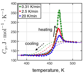
A separate, calorimetric study due to Eastel et al. [18] does report a range of preparation protocols. We replot their heat capacity data per stoichiometric unit in Fig. S3, where we also provide smooth fits. The fits employ ad hoc functional forms. For heating (solid lines), we have:
| (S11) |
where the trial function is given by
| (S12) |
We fix the specific heat at K at the value J(molK) and at K at the value J(molK). Subsequently, , , , , are determined by fitting. For cooling we use the form:
| (S13) |
where trial function is given by
| (S14) |
with , , as fitting parameters.
We list below the resulting values of the peak values of the excess heat capacity of the melt relative to the glass:
| Cooling rate, K/min | , J/(molK) |
|---|---|
We use the cooling part of the protocol to infer J/(molK) for As2Se3, which is in agreement with Wagner et al. [19] According to the latter work, J/(molK) for As2S3. These values, listed in the Table below, are used to evaluate the low bound in Eq. 4.
| material | , J/(molK) | , J/K | , K | , K |
|---|---|---|---|---|
| As2Se3 | 65 | 31.4 | 450 | |
| As2S3 | 62 | 24.5 | 465 | 265 |
We approximate the value of the configurational entropy as , where is the entropy of melting of the corresponding crystal. This approximation is based on two established notions: On the one hand, the configurational entropy, at the glass transition, varies within a modest range [20, 21, 22, 23] per bead. On the other hand, the number of beads for a compound can be determined by calibrating its fusion entropy to that of the Lennard-Jones liquid [21, 22], viz. . Thus we use , where is the fusion enthalpy ( kJ/mol (As2Se3), kJ/mol (As2S3) [24]) and is the melting temperature ( K (As2Se3), K (As2S3) [24]). We list the resulting values of in the Table above, as well as values of [16, 25] and the Kauzmann temperature , as reported in Ref. [26], to be used in evaluating Eqs. S18 and S19.
II.2 predictions: Numerical estimates
We do not have data on the dimensionless rate of decrease of the bulk modulus with temperature for either As2Se3 or As2S3. The quantity is, however, not expected to be too different from negative unity, judging from data on a different intermetallic compound [27]. Thus we estimate Eq. 4 of the main text for two specific values of viz. and , respectively, , to get a quantitative feel for the significance of the thermally-induced changes of the elastic response. Thus we compute two quantities, as pertinent to Eq. 4:
| (S15) |
| (S16) |
As an alternative to the fragility-based estimate in Eq. 7 of main text, one may also use the conventional parameterization [28, 21] , where is the so called Kauzmann temperature. For known glassformers, [29, 21]. Assuming at , one obtains straightforwardly
| (S17) |
Thus one may evaluate the following two lower bounds on :
| (S18) |
and
| (S19) |
Numerical estimates of the expressions in Eqs. S15, S16, S18 and S19 are given in the Table below:
| material | , eV | , eV | , eV | , eV |
| As2Se3 | 0.041 | 0.054 | ||
| As2S3 | 0.080 | 0.093 | 0.049 | 0.062 |
Of the four options, we regard the quantity from Eq. S16 as the most reliable estimate and, hence, present it as our predicted value in the main text. We see that not knowing the value of translates to at most a 15% uncertainty in the first place.
Eq. 7 in the main text and Eqs. S18 and S19 are very simple algebraically but, at the same time, are subject to greater uncertainty than the .
Eq. 7 only give a lower bound and requires one to independently determine the actual, not apparent barrier for -relaxation. This can be done indirectly, by measuring the apparent activation barrier above and below the glass transition, respectively and then applying the the formalism presented in Ref. [30]. For the sake of a quick estimate, one may use the available fragility data for the selenide from Ref. [31], whose authors report a fragility coefficient at K. Adopting , one obtains eV for the dynamic range , eV for . This is consistent with Eqs. (7) being a lower bound.
Moving onto Eqs. S18 and S19, the Kauzmann temperature is a fiducial temperature at which the configurational entropy would vanish. It is determined in two steps [32]: First one must subtract the entropy of a frozen glass from that of the equilibrated melt. We do not know the entropy of the glass but expect it to be numerically close to that of the corresponding crystal. There is, however, some uncertainty stemming from the free energy minima in glasses being separated by finite barriers in finite dimensions. In physical terms, this means that the glass might have additional degrees of freedom, including in particular the boson peak and two-level systems [5, 33, 34, 35], that might meaningfully contribute to its entropy, even though the contribution is expected to be modest [36]. Once evaluated, the configurational entropy must be extrapolated below the glass transition temperature to determine the temperature where it would vanish, which introduces further uncertainty. While the overall trend for the values of predicted using calorimetry and kinetics, respectively, clearly points out the two quantities are equal, individual substances may deviate from this trend substantially [28, 32, 22, 23].
III Conductivity prefactor
Here we perform basic estimates for polaron-based mechanisms of electrical conduction, in which transport occurs via activated hops. First, we reproduce the expression from the main text for the conductivity in the present scenario
| (S20) |
where for concreteness we assume that the hole polarons are the dominant charge carriers [37, 38]. The insulating gap depends on the temperature, the dependence well approximated by a linear law within the temperature range in question [9]:
| (S21) |
According to our earlier work [9], both edges of the insulating gap contribute to the temperature dependence of the insulating gap. The contribution of the temperature-dependent part of the gap to the prefactor in the conductivity is bounded from above by the quantity . Thus we proceed to estimate
| (S22) |
For the four substances considered in Ref. [9], the quantity varies within the range to . We adopt the lower value , since the r.h.s. of the equation above is an upper bound. Near the glass transition, nm [3, 5, 32]. The fraction is of order one. The effective charge of the polaron is numerically close to the electron charge, but is actually less, owing to the polarization of the lattice [4]. Having this reduction in the effective charge in mind and setting nm yields a prefactor of order or less, in agreement with Fig. 1 of the main text.
If aging causes a relaxation in the electronic structure, there will be an additional contribution to for aged samples. Assume, again, that the dominant charge carrier is holes. It is conceivable that the Urbach tail states, which are candidate states for polarons [4], will relax relative to the edge of the valence band. We anticipate that this contribution would be much smaller than the present predictions for . Indeed, stabilization of electronic levels would have to be a small quotient of the enthalpy of melting per electron, which is roughly or so for chalcogenides; here is the melting temperature. Indeed, the entropy of melting is rather universally per atom [24] and the number of valence electrons, on the average, is close to five. In contrast, the predicted value of can be no smaller than even for the strongest known substances. These notions are consistent with a reported insensitivity of the optical edge to heat treatment [39].
It is instructive to compare the prefactor in Eq. 3 of main text to that arising in Emin’s small polaron picture [37], viz., . Here, is the volumetric size of an atom, up to a constant of order one, and is a generic bond-vibrational frequency. Assuming, as before, that local vibrations are not sensitive to freezing, the apparent activation energy will exhibit a jump in its -dependence, across the glass transition, because the lattice constant will increase with temperature at different rates, below and above the glass transition, respectively. One may show straightforwardly that
| (S23) |
where is the thermal expansion coefficient. This yields eV for As2Se3, for which K-1 and K-1, respectively [40]. We see the volumetric effect is two orders of magnitude less than the effect of the arrest of dynamics, below the glass transition, because the density depends on temperature too weakly in the first place. In Emin’s small polaron scenario, the prefactor would be increased, relative to the estimate above, by the factor or so. This is not a significant difference, in view of the approximate nature of the estimate in the first place.
References
- Heeger et al. [1988] A. J. Heeger, S. Kivelson, J. R. Schrieffer, and W. P. Su, Rev. Mod. Phys. 60, 781 (1988).
- Rice and Mele [1982] M. J. Rice and E. J. Mele, Phys. Rev. Lett. 49, 1455 (1982).
- Zhugayevych and Lubchenko [2010a] A. Zhugayevych and V. Lubchenko, J. Chem. Phys. 132, 044508 (2010a).
- Lukyanov et al. [2018] A. Lukyanov, J. C. Golden, and V. Lubchenko, J. Phys. Chem. B 122, 8082 (2018).
- Lubchenko and Wolynes [2001] V. Lubchenko and P. G. Wolynes, Phys. Rev. Lett. 87, 195901 (2001).
- Zhugayevych and Lubchenko [2010b] A. Zhugayevych and V. Lubchenko, J. Chem. Phys. 133, 234504 (2010b).
- Golden et al. [2017] J. C. Golden, V. Ho, and V. Lubchenko, J. Chem. Phys. 146, 174502 (2017).
- Takayama et al. [1980] H. Takayama, Y. R. Lin-Liu, and K. Maki, Phys. Rev. B 21, 2388 (1980).
- Lubchenko and Kurnosov [2019] V. Lubchenko and A. Kurnosov, J. Chem. Phys. 150, 244502 (2019).
- Su and Schrieffer [1980] W. P. Su and J. R. Schrieffer, Proc. Natl. Acad. Sci. U. S. A. 77, 5626 (1980).
- Brazovskii and Kirova [1981] S. Brazovskii and N. Kirova, JETP Lett. 33, 4 (1981).
- Emin [1980] D. Emin, Electrical and optical properties of amorphous thin films, in Polycrystalline and Amorphous Thin Films and Devices, edited by L. L. Kazmerski (Academic Press, New York, 1980) p. 17.
- Campbell and Bishop [1982] D. K. Campbell and A. R. Bishop, Nuclear Physics B 200, 297 (1982).
- Davey and Baker [1983] T. C. Davey and E. H. Baker, J. Mater. Sci. 18, 717 (1983).
- Bobb et al. [1975] L. C. Bobb, H. H. Byer, and K. Kramer, Electrical properties of As2S3 glass, techreport (Pitman-Dunn Laboratory, U.S. ARMY ARMAMENT COMMAND, FRANKFORD ARSENAL, PHILADELPHIA, PENNSYLVANIA 19137, 1975) https://apps.dtic.mil/sti/citations/tr/ADA020552.
- Seager and Quinn [1975] C. H. Seager and R. K. Quinn, J. Non-Cryst. Sol. 17, 386 (1975).
- Borisova [1981] Z. U. Borisova, Glassy semiconductors (Plenum Press, New York, 1981).
- Eastel et al. [1977] A. J. Eastel, J. A. Wilder, R. K. Mohr, and C. T. Moynihan, J. Amer. Ceramic Soc. 60, 134 (1977).
- Wagner et al. [1998] T. Wagner, S. O. Kasap, M. Vlcek, A. Sklenár, and A. Stronski, J. Mater. Sci. 33, 5581 (1998).
- Xia and Wolynes [2000] X. Xia and P. G. Wolynes, Proc. Natl. Acad. Sci. U. S. A. 97, 2990 (2000).
- Lubchenko and Wolynes [2003a] V. Lubchenko and P. G. Wolynes, J. Chem. Phys. 119, 9088 (2003a).
- Rabochiy et al. [2013] P. Rabochiy, P. G. Wolynes, and V. Lubchenko, J. Phys. Chem. B 117, 15204 (2013).
- Lubchenko and Rabochiy [2014] V. Lubchenko and P. Rabochiy, J. Phys. Chem. B 118, 13744 (2014).
- Haynes [2015] W. M. Haynes, ed., CRC Handbook of Chemistry and Physics, 96th Edition (CRC Press, Boca Raton, 2015).
- Kolomiets [1964] B. T. Kolomiets, physica status solidi (b) 7, 713 (1964).
- Tatsumisago et al. [1990] M. Tatsumisago, B. L. Halfpap, J. L. Green, S. M. Lindsay, and C. A. Angell, Phys. Rev. Lett. 64, 1549 (1990).
- Gadaud and Pautrot [2003] P. Gadaud and S. Pautrot, J. Non-Cryst. Sol. 316, 146 (2003).
- Richert and Angell [1998] R. Richert and C. A. Angell, J. Chem. Phys. 108, 9016 (1998).
- Wang and Angell [2003] L.-M. Wang and C. A. Angell, J. Chem. Phys. 118, 10353 (2003).
- Lubchenko and Wolynes [2004] V. Lubchenko and P. G. Wolynes, J. Chem. Phys. 121, 2852 (2004).
- Koštál et al. [2024] P. Koštál, M. Včeláková, and J. Málek, J. Am. Ceram. Soc. 107, 844 (2024).
- Lubchenko [2015] V. Lubchenko, Adv. Phys. 64, 283 (2015).
- Lubchenko and Wolynes [2003b] V. Lubchenko and P. G. Wolynes, Proc. Natl. Acad. Sci. U. S. A. 100, 1515 (2003b).
- Lubchenko [2018] V. Lubchenko, Advances in Physics: X 3, 1510296 (2018).
- Lubchenko and Wolynes [2007] V. Lubchenko and P. G. Wolynes, Adv. Chem. Phys. 136, 95 (2007), https://arxiv.org/abs/cond-mat/0506708.
- Eastwood and Wolynes [2002] M. P. Eastwood and P. G. Wolynes, Europhys. Lett. 60, 587 (2002).
- Emin [1983a] D. Emin, Comments Solid State Phys. 11, 35 (1983a).
- Emin [1983b] D. Emin, Comments Solid State Phys. 11, 59 (1983b).
- Arai et al. [1975] T. Arai, S. Komiya, and K. Kudo, JNC 18, 295 (1975).
- Voronova et al. [2001] A. E. Voronova, V. A. Ananichev, and L. N. Blinov, Glass Phys. Chem. 27, 267 (2001).