Simplifying Deep Temporal Difference Learning

Abstract

$Q$-learning played a foundational role in the field reinforcement learning (RL). However, TD algorithms with off-policy data, such as $Q$-learning, or nonlinear function approximation like deep neural networks require several additional tricks to stabilise training, primarily a replay buffer and target networks. Unfortunately, the delayed updating of frozen network parameters in the target network harms the sample efficiency and, similarly, the replay buffer introduces memory and implementation overheads. In this paper, we investigate whether it is possible to accelerate and simplify TD training while maintaining its stability. Our key theoretical result demonstrates for the first time that regularisation techniques such as LayerNorm can yield provably convergent TD algorithms without the need for a target network, even with off-policy data. Empirically, we find that online, parallelised sampling enabled by vectorised environments stabilises training without the need of a replay buffer. Motivated by these findings, we propose PQN, our simplified deep online $Q$-Learning algorithm. Surprisingly, this simple algorithm is competitive with more complex methods like: Rainbow in Atari, R2D2 in Hanabi, QMix in Smax, PPO-RNN in Craftax, and can be up to 50x faster than traditional DQN without sacrificing sample efficiency. In an era where PPO has become the go-to RL algorithm, PQN reestablishes $Q$-learning as a viable alternative. We make our code available at: https://github.com/mttga/purejaxql

1 Introduction

In reinforcement learning (RL), the challenge of developing simple, efficient and stable algorithms remains open. Temporal difference (TD) methods have the potential to be simple and efficient, but are notoriously unstable when combined with either off-policy sampling or nonlinear function approximation [76]. Starting with the introduction of the seminal deep $Q$-network (DQN)[52], many tricks have been developed to stabilise TD for use with deep neural network function approximators, most notably: the introduction of a replay buffer [52], target networks [53], trust region based methods [65], double Q-networks [78, 23], maximum entropy methods [26, 27] and ensembling [14]. Out of this myriad of algorithmic combinations, proximal policy optimisation (PPO) [66] has emerged as the de facto choice for RL practitioners, proving to be a strong and efficient baseline across popular RL domains. Unfortunately, PPO is far from stable and simple: PPO does not have provable convergence properties for nonlinear function approximation and requires extensive tuning and additional tricks to implement effectively [33, 20].

Recent empirical studies [47, 48, 9] provide evidence that TD can be stabilised without target networks by introducing regularisation such as BatchNorm [35] and LayerNorm [2] into the $Q$-function approximator. Little is known about why these techniques work or whether they have unintended side-effects. Motivated by these findings, we ask: are regularisation techniques such as BatchNorm and LayerNorm the key to unlocking simple, efficient and stable RL algorithms? To answer this question, we provide a rigorous analysis of regularised TD. We summarise our core theoretical insights as: I) introducing BatchNorm in TD methods can lead to myopic behaviour if not applied carefully to a function approximator, and II) introducing LayerNorm and $\ell_{2}$ regularisation into the $Q$-function approximator leads to provable convergence, stabilising nonlinear, off-policy TD without the need for target networks and without the myopic behaviour of BatchNorm.

Guided by these insights, we develop a modern value-based TD method which we call a parallelised $Q$-network (PQN): for simplicity, we revisit the original $Q$-learning algorithm [81], which updates a $Q$-function approximator online without a target network. A recent breakthrough in RL has been running the environment and agent jointly on the GPU [49, 25, 46, 51, 63, 41]. However, the replay buffer’s large memory footprint makes pure-GPU training impractical with traditional DQN. With the goal of enabling $Q$-learning in pure-GPU setting, we propose replacing the replay buffer with an online synchronous update across a large number of parallel environments. For stability, we integrate our theoretical findings in the form of a normalised deep $Q$ network. We provide a schematic of our proposed PQN algorithm in Fig. 1(d).

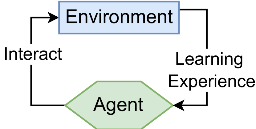
(a) Online $Q$-Learning

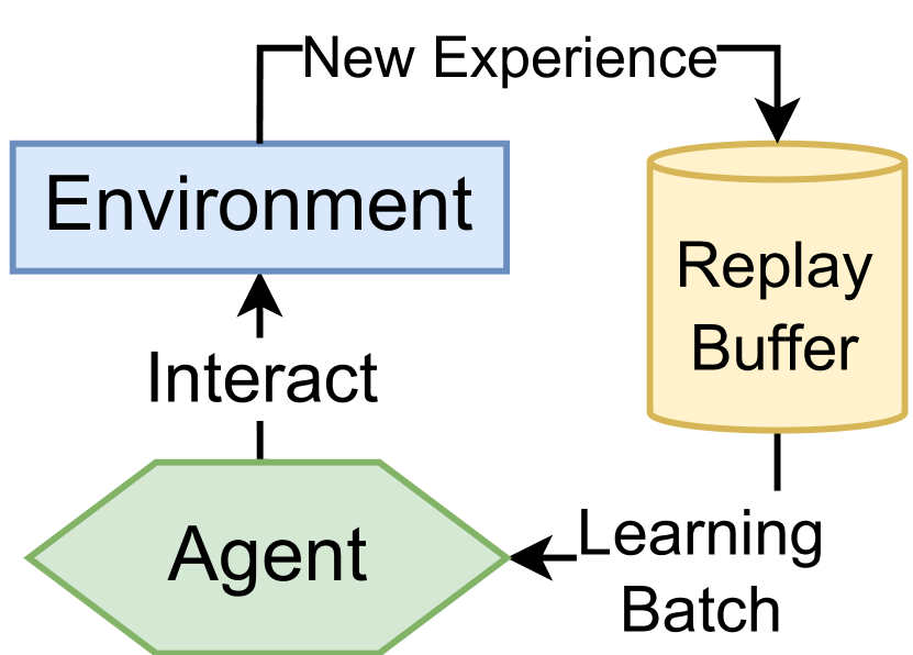
(b) DQN

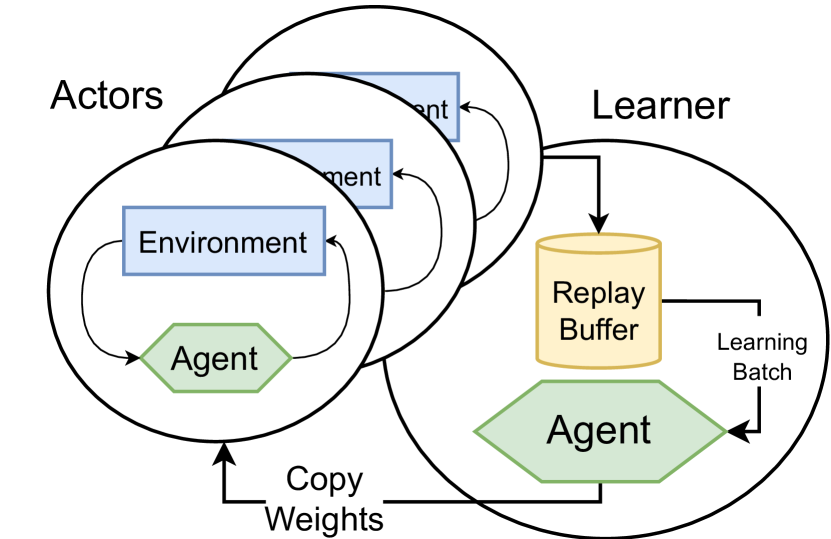
(c) Distributed DQN

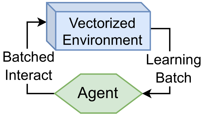
(d) PQN

Figure 1: Classical $Q$-Learning directly interacts with the environment and trains on each transition. In contrast, DQN stores experiences in a replay buffer and performs gradient updates using minibatches sampled from this buffer. Distributed DQN enhances this approach by collecting experiences in parallel threads, while a separate process continually trains the agent. PQN operates similarly to classical online $Q$-Learning, but conducts interactions and learning in batches.

To validate our theoretical results, we evaluated PQN in Baird’s counterexample, a challenging domain that is provably divergent for off-policy methods [4]. Our results show that PQN can converge where non-regularised variants fails. We provide an extensive empirical evaluation to test the performance of PQN in single-agent and multi-agent settings. Despite its simplicity, we found this algorithm competitive in a range of tasks. Notably, PQN achieves high performances in just a few hours in many games of the Arcade Learning Environment (ALE) [6], competes effectively with PPO on the open-ended Craftax task [50], and stands alongside state-of-the-art Multi-Agent RL (MARL) algorithms, such as R2D2-VDN in Hanabi [5] and Qmix in Smax [63]. Despite not sampling from past experiences in a replay buffer, the faster convergence of PQN demonstrates that the sample efficiency loss can be minimal. This positions PQN as a strong method for efficient and stable RL in the age of deep vectorised Reinforcement Learning (DVRL).

We summarise our empirical contributions: I) we propose PQN, a simplified, parallelised, and normalised version of DQN which eliminates the use of both the replay buffer and the target network; II) we demonstrate that PQN is fast, stable, simple to implement, uses few hyperparameters, and is compatible with pure-GPU training and temporal-based networks such as RNNs, and III) our extensive empirical study demonstrates PQN achieves competitive results in significantly less wall-clock time than existing state-of-the-art methods.

2 Preliminaries

We now formalise our problem setting in the context of vectorised environments before introducing the necessary theoretical and regularisation tools for our analysis. We provide a discussion of related work in Appendix B. We denote the set of all probability distributions on a set $\mathcal{X}$ as $\mathcal{P}(\mathcal{X})$.

2.1 Reinforcement Learning

In this paper, we consider the infinite horizon discounted RL setting, formalised as a Markov Decision Process (MDP) [7, 59]: $\mathcal{M}\coloneqq\langle\mathcal{S},\mathcal{A},P_{S},P_{0},P_{R},\gamma\rangle$ with state space $\mathcal{S}$, action space $\mathcal{A}$, transition distribution $P_{S}:\mathcal{S}\times\mathcal{A}\to\mathcal{P}(\mathcal{S})$, initial state distribution $P_{0}\in\mathcal{P}(\mathcal{S})$, bounded stochastic reward distribution $P_{R}:\mathcal{S}\times\mathcal{A}\to\mathcal{P}([-r_{max},r_{max}])$ where $r_{max}\in\mathbb{R}<\infty$ and scalar discount factor $\gamma\in[0,1)$. An agent in state $s_{t}\in\mathcal{S}$ taking action $a_{t}\in\mathcal{A}$ observes a reward $r_{t}\sim P_{R}(s_{t},a_{t})$. The agent’s behaviour is determined by a policy that maps a state to a distribution over actions: $\pi:\mathcal{S}\to\mathcal{P}(\mathcal{A})$ and the agent transitions to a new state $s_{t+1}\sim P_{S}(s_{t},a_{t})$. As the agent interacts with the environment through a policy $\pi$, it follows a trajectory $\tau_{t}\coloneqq(s_{0},a_{0},r_{0},s_{1},a_{1},r_{1},\dots s_{t-1},a_{t-1},r_{t-1},s_{t})$ with distribution $P^{\pi}_{t}$. For simplicity, we denote state-action pair $x_{t}\coloneqq(s_{t},a_{t})\in\mathcal{X}$ where $\mathcal{X}\coloneqq\mathcal{S}\times\mathcal{A}$. The state-action pair transitions under policy $\pi$ according to the distribution $P_{X}^{\pi}:\mathcal{X}\rightarrow\mathcal{X}$.

The agent’s goal is to learn an optimal policy of behaviour $\pi^{\star}\in\Pi^{\star}$ by optimising the expected discounted sum of rewards over all possible trajectories $J^{\pi}$, where: $\Pi^{\star}\coloneqq\operatorname*{arg\,max}_{\pi}J^{\pi}$ is an optimal policy for the objective $J^{\pi}\coloneqq\mathbb{E}_{\tau_{\infty}\sim P_{\infty}}\left[\sum_{t=0}^{\infty}\gamma^{t}r_{t}\right]$. The expected discounted reward for an agent in state $s_{t}$ for taking action $a_{t}$ is characterised by a $Q$-function, which is defined recursively through the Bellman equation: $Q^{\pi}(x_{t})=\mathcal{B}^{\pi}[Q^{\pi}](x_{t})$, where the Bellman operator $\mathcal{B}^{\pi}$ projects functions forwards by one step through the dynamics of the MDP: $\mathcal{B}^{\pi}[Q^{\pi}](x_{t})\coloneqq\mathbb{E}_{x_{t+1}\sim P_{X}^{\pi}(x_{t}),r_{t}\sim P(x_{t})}\left[r_{t}+\gamma Q^{\pi}(x_{t+1})\right]$. Of special interest is the $Q$-function for an optimal policy $\pi^{\star}$, which we denote as $Q^{\star}(x_{t})\coloneqq Q^{\pi_{\star}}(x_{t})$. The optimal $Q$-function satisfies the optimal Bellman equation $Q^{\star}(x_{t})=\mathcal{B}^{\star}[Q^{\star}](x_{t})$, where $\mathcal{B}^{\star}$ is the optimal Bellman operator: $\mathcal{B}^{\star}[Q^{\star}](x_{t})\coloneqq\mathbb{E}_{s_{t+1}\sim P_{S}(x_{t}),r_{t}\sim P(x_{t})}\left[r_{t}+\gamma\max_{a^{\prime}}Q^{\star}(s_{t+1},a^{\prime})\right]$.

As an optimal policy can be constructed from the optimal $Q$ function by taking a greedy action $a_{t}^{\star}\in\operatorname*{arg\,max}_{a^{\prime}}Q^{\star}(s_{t},a^{\prime})$ in each state $s_{t}$, learning an optimal $Q$-function is sufficient for solving the RL problem. Approaches that estimate $Q$-functions directly are known as model-free approaches as they do not require a model of environment dynamics. In all but the simplest discrete MDPs, some form of $Q$ function approximation $Q_{\phi}:\mathcal{X}\to\mathbb{R}$ parametrised by $\phi\in\Phi$ is required to represent the space of $Q$-functions. For sake of analysis, we assume $\Phi$ is convex.

2.2 Vectorised Environments

In the context of DVRL, all interactions between an agent and a vectorised environment contain a batch dimension: the agent receives $n$ observations, produces $n$ actions, and receives $n$ rewards, where $n$ is the number of parallel environments. In classical frameworks like Gymnasium [75], this is achieved with multi-threading and a batching layer that aggregates the information. However, in more recent GPU-based frameworks like IsaacGym [49], ManiSkill2 [25] Jumanji [10], Craftax [51], JaxMARL [63] and so on, operations are truly vectorised, meaning that a single hardware processes the parallel environments using batched tensors. This allows an agent to interact with thousands of environments, without copying parameters on different nodes or cores, and enables end-to-end GPU learning pipelines, which can accelerate the training of PPO agents by orders of magnitude [49, 82, 25, 46]. End-to-end single-GPU training is not compatible with traditional off-policy methods for two reasons: firstly keeping a replay buffer in GPU memory is not possible in complex environments, as it would occupy most of the memory, and secondly, convergence of off-policy methods demands a very high number of updates in respect to the sampled experiences (DQN performs traditionally one gradient step per each environment step) which is impractical unless learning occurs in a different parallel process (see Fig. 1(c)). For this reason, all referenced frameworks provide mainly PPO or A2C baselines, i.e. DVRL is missing a $Q$-learning baseline.

2.3 Temporal Difference Methods

Many RL algorithms employ TD learning for policy evaluation, which combines bootstrapping, state samples and sampled rewards to estimate the expectation in the Bellman operator [71]. In their simplest form, TD methods update the function approximation parameters according to:

$$\phi_{i+1}=\phi_{i}+\alpha_{i}\left(r+\gamma Q_{\phi_{i}}(x^{\prime})-Q_{\phi_{i}}(x)\right)\nabla_{\phi}Q_{\phi_{i}}(x),$$ (1)

where $x\sim d^{\mu},r\sim P_{R}(x),x^{\prime}\sim P_{X}^{\pi}(x)$. Here $d^{\mu}\in\mathcal{P}(\mathcal{X})$ is a sampling distribution, and $\mu$ is a sampling policy that may be different from the target policy $\pi$. Methods for which the sampling policy differs from the target policy are known as off-policy methods. In this paper, we will study on the $Q$-learning [81, 17] TD update:

$$\phi_{i+1}=\phi_{i}+\alpha_{i}\left(r+\gamma\sup_{a^{\prime}}Q_{\phi_{i}}(s^{\prime},a^{\prime})-Q_{\phi_{i}}(x)\right)\nabla_{\phi}Q_{\phi_{i}}(x),$$ (2)

which aims to learn an optimal $Q$-function by estimating the optimal Bellman operator. As data in $Q$-learning is gathered from an exploratory policy $\mu$ that is not optimal, $Q$-learning is an inherently off-policy algorithm.

For simplicity of notation we define the tuple $\varsigma\coloneqq(x,r,x^{\prime})$ with distribution $P_{\varsigma}$ and the TD-error vector as:

$$\delta(\phi,\varsigma)\coloneqq\left(r+\gamma Q_{\phi}(x^{\prime})-Q_{\phi}(x)\right)\nabla_{\phi}Q_{\phi}(x),$$ (3)

allowing us to write the TD parameter update as: $\phi_{i+1}=\phi_{i}+\alpha_{i}\delta(\phi_{i},\varsigma)$. Typically, $d^{\mu}$ is the stationary state-action distribution of an ergodic Markov chain but may be another offline distribution such as a distribution induced by a replay buffer:

Assumption 1 (TD Sampling).

When updating TD, $x\sim d^{\mu}$ is either sampled i.i.d. from a distribution with support over $\mathcal{X}$ or is sampled from an ergodic Markov chain with stationary distribution $d^{\mu}$ defined over a $\sigma$-algebra that is countably generated from $\mathcal{X}$.

We denote the expected TD-error vector as: $\delta(\phi)\coloneqq\mathbb{E}_{\varsigma\sim P_{\varsigma}}[\delta(\phi,\varsigma)]$ and define the set of TD fixed points as: $\phi^{\star}\in\left\{\phi|\delta(\phi)=0\right\}$. If a TD algorithm converges, it must converge to a TD fixed point as the expected parameter update is zero for all $\phi^{\star}$.

2.4 Analysis of TD

As TD updates aren’t a gradient of any objective, they fall under the more general class of algorithms known as stochastic approximation [62, 11]. Stability is not guaranteed in the general case and convergence of TD methods has been studied extensively [80, 76, 15, 8, 68]. Fellows et al. [21] show that for function approximators for which the Jacobian $\nabla_{\phi}\delta(\phi)$ is defined almost everywhere, stability is determined by the Jacobian eigenvalues (see Appendix C for a detailed exposition). This naturally leads to two causes of instability in TD methods:

Off-policy Instability

TD can become unstable if:

$$\gamma v^{\top}\mathbb{E}_{\varsigma\sim P_{\varsigma}}\left[\nabla_{\phi}Q_{\phi}(x^{\prime})\nabla_{\phi}Q_{\phi}(x)^{\top}\right]v<v^{\top}\mathbb{E}_{x\sim d^{\mu}}\left[\nabla_{\phi}Q_{\phi}(x)\nabla_{\phi}Q_{\phi}(x)^{\top}\right]v,$$ (4)

does not hold for any unit test vector $v$. Unfortunately, Condition 4 can only be shown to hold in the on-policy sampling regime when $d^{\mu}=d^{\pi}$ is the stationary distribution of the MDP. This is because the Cauchy-Schwartz inequality needed to prove $\gamma\lVert\nabla_{\phi}Q_{\phi}(x^{\prime})\nabla_{\phi}Q_{\phi}(x)^{\top}\|\leq\lVert\nabla_{\phi}Q_{\phi}(x)\nabla_{\phi}Q_{\phi}(x)^{\top}\|$ does not hold for arbitrary off-policy sampling distributions $d^{\mu}$ [21]. Hence off-policy sampling is a key source of instability in TD, especially in algorithms such as $Q$-learning.

Nonlinear Instability

TD can become unstable if:

$$\mathbb{E}_{\varsigma\sim P_{\varsigma}}\left[(r+\gamma Q_{\phi}(x^{\prime})-Q_{\phi}(x))v^{\top}\nabla_{\phi}^{2}Q_{\phi}(x)v\right]<0,$$ (5)

does not hold for any unit test vector $v$. Condition 5 does not apply in the linear case as second order derivatives are zero. In the nonlinear case, the left hand side of Inequality 5 can be arbitrarily positive depending upon the specific MDP and choice of function approximator. Hence nonlinearity is a key source of instability in TD. Together both off-policy and nonlinear instability formalise the deadly triad [72, 77] and TD can be unstable if either conditions are not satisfied.

3 Analysis of Regularised TD

Proofs for all theorems and corollaries can be found in Appendix D

We now use the techniques of Section 2.4 to provide an analysis of regularised TD, confirming our theoretical hypothesis that careful application of techniques such as LayerNorm and $\ell_{2}$ regularisation can stabilise TD. Recalling that $x\coloneqq\{s,a\}$, we remark that our results can be derived for value functions by setting $x=s$ in our analysis.

3.1 BatchNorm TD is Myopic

We begin by investigating BatchNorm regularisation, which is essential for stabilising algorithms such as CrossQ [9]. We ask: ‘Are there any side effects of using BatchNorm?’ To answer this question, we study a $Q$-function approximator with a final BatchNorm layer of the form:

$$Q_{\phi}(x)=w^{\top}\textrm{BatchNorm}_{N}[f](x),$$ (6)

where $f:\mathcal{X}\rightarrow\mathbb{R}^{k}$ is any measurable (i.e. very general) function and $w\in\mathbb{R}^{k}$ is a vector of weights for the final linear layer of the approximator. Typically $f(x)$ is a deep neural network which may also include BatchNorm layers. As the number of batch samples $N$ increases, BatchNorm’s empirical mean and variance better approximate the true mean and variance of the data, thereby improving regularisation. Unfortunately in the same limit, the Bellman operator for BatchNorm $Q$-functions becomes myopic:

Theorem 1.

Under 1, using the BatchNorm $Q$-function defined in Eq. 6 $\lim_{N\rightarrow\infty}\mathbb{E}_{x_{t}\sim d^{\mu}}\left[\mathcal{B}\left[Q_{\phi}\right](x_{t})\right]=\mathbb{E}_{r\sim P_{R}(x_{t}),x_{t}\sim d^{\mu}}\left[r\right]$ almost surely.

Theorem 1 reveals that as batchsize $N$ increases, agents learning a BatchNorm $Q$-function prioritise immediate reward over long term returns. Mathematically, this issue arises because BatchNorm’s empirical expectation is taken across the observed data, causing the final linear layer to tend to zero: $w^{\top}(\mathbb{E}[f(x)]-\mu_{N})\rightarrow 0$. Strengthening the BatchNorm thus makes an agent’s behaviour more myopic as the Bellman operator no longer accounts for how reward propagates through the dynamics of the MDP. Myopic agents perform poorly in tasks where planning to obtain longer term goals is required, for example in sparser domains where reward signal is withheld for several timesteps of interaction. In real-world applications, it is often difficult to specify a dense reward signal towards task completion, and so we caution against the use of BatchNorm in practice, especially if applied before the final linear network layer. We observe this behaviour in our empirical evaluation in Section 5.1.

3.2 LayerNorm + $\ell_{2}$ Mitigates Off-Policy Instability

Is there an alternative method that retains the stabilising power of BatchNorm without the limiting myopic behaviour? In this paper, we propose LayerNorm as a viable option. Unlike BatchNorm, LayerNorm does not suffer from a myopic Bellman operator as the expectation is taken across a layer’s output vector rather than across the batch data. To understand how LayerNorm stabilises TD, we study the following $Q$-function approximator with a $k$-width LayerNorm activation and a single hidden layer:

$$\vspace{-0.5cm}Q_{\phi}(x)=w^{\top}\textrm{ReLU}\circ\textrm{LayerNorm}\left[Mx\right].$$ (7)

Here $\phi\coloneqq\{w,M\}$ where $M\in\mathbb{R}^{k\times d}$ is a $k\times d$ matrix and $w\in\mathbb{R}^{k}$ is a vector of final layer weights. Deeper networks with more LayerNorm layers may be used in practice, however our analysis reveals that only the final layer weights affect the stability of TD with wide LayerNorm function approximators. We make the following mild regularity assumptions:

Assumption 2 (Network Regularity Assumptions).

We assume that the parameter space $\Phi$ is convex with $\lVert\phi\rVert<\infty$ almost surely and parameters are initialised i.i.d.

This assumption can be trivially adhered to by sampling the initial network weights from a Gaussian distribution with finite mean and variance. As the expectation is taken across network width in LayerNorm, the effect of regularisation is increased for wide critics as $k\rightarrow\infty$. We now study how LayerNorm mitigates the off-policy instability condition (Eq. 4) in this limit:

Theorem 2.

Under 2, using the $k$-width LayerNorm $Q$-function defined in Eq. 7:

$$\frac{\gamma v^{\top}\nabla_{\phi}Q_{\phi}(x^{\prime})\nabla_{\phi}Q_{\phi}(x)^{\top}v-(v^{\top}\nabla_{\phi}Q_{\phi}(x))^{2}}{\lVert v\rVert^{2}}\leq\left(\frac{\gamma}{2}\right)^{2}+\mathcal{O}\left(\frac{1}{\sqrt{k}}\right),\vspace{-0.2cm}$$ (8)

almost surely for any test vector $v\in\Phi$ and any state-action transition pair $x,x^{\prime}\in\mathcal{X}$.

Crucially, the bound in Eq. 8 does not depend on the sampling distribution $d^{\mu}$. Mathematically, this is due to the normalising property: $\lVert\textrm{LayerNorm}[Mx]\rVert\leq 1$, which is independent of the input data. In contrast, a wide neural network without LayerNorm would tend towards a linearised form $Q_{\phi_{0}}(x)+\nabla_{\phi}Q_{\phi_{0}}(x)^{\top}(\phi-\phi_{0})$ [42] which is data dependent and still suffers from off-policy instability like all linear function approximators in the off-policy regime: recall from Section 2.4, the Cauchy-Schwartz inequality required to prove the stability condition $\gamma\lVert\nabla_{\phi}Q_{\phi}(x^{\prime})\nabla_{\phi}Q_{\phi}(x)^{\top}\|\leq\lVert\nabla_{\phi}Q_{\phi}(x)\nabla_{\phi}Q_{\phi}(x)^{\top}\|$ can only be guaranteed to hold if $d^{\pi}=d^{\mu}$.

The key insight from Theorem 2 is that by using LayerNorm, we can always mitigate the effects of off-policy instability in TD: increasing LayerNorm width $k$ and introducing $\ell_{2}$ regularisation over weights $w$ of magnitude $-w\left(\frac{\gamma}{2}\right)^{2}$ to make the bound in Eq. 8 negative ensures the TD stability criterion holds regardless of any off-policy sampling regime or specific MDP.

3.3 LayerNorm Mitigates Nonlinear Instability

We investigate how LayerNorm mitigates instability arising from nonlinear function approximation:

Theorem 3.

Under 2, using the LayerNorm $Q$-function defined in Eq. 7 $\nicefrac{{1}}{{\lVert v\rVert^{2}}}\left\lvert\left(r+\gamma Q_{\phi}(x^{\prime})-Q_{\phi}(x)\right)v^{\top}\nabla_{\phi}^{2}Q_{\phi}(x)v\right\rvert=\mathcal{O}\left(\nicefrac{{1}}{{\sqrt{k}}}\right)$, almost surely for any test vector and any state-action transition pair $x,x^{\prime}\in\mathcal{X}$.

Theorem 3 proves nonlinear instability tends to zero with increasing LayerNorm regularisation. For a suitably wide critic the only form of instability that we need to account for is the off-policy instability and only in the final layer weights. As proposed in Section 3.2, this can be mitigated using simple $\ell_{2}$ regularisation if necessary. We now formally confirm this intuition:

Corollary 3.1.

Define the $\ell_{2}$-regularised TD update as $\delta_{\textnormal{{reg}}}(\phi,\varsigma)\coloneqq\delta(\phi,\varsigma)-\left(\frac{\gamma}{2}\right)^{2}[w^{\top}\ 0\ \cdots 0]^{\top}.$ Under 2, using the LayerNorm $Q$-function defined in Eq. 7, for any $\eta\geq 1$ there exists some finite $k$ such that the TD Jacobian has negative eigenvalues almost surely.

In Section 5.1 we test our theoretical claim in Corollary 3.1 empirically, demonstrating that LayerNorm + $\ell_{2}$ regularisation can stabilise Baird’s counterexample, an MDP intentionally designed to cause instability for TD. We remark that whilst adding an $\ell_{2}$ regularisation term $-\eta\phi$ to all parameters can stabilise TD in principle, large $\eta$ recovers a quadratic optimisation problem with minimum at $\phi=0$, pulling the TD fixed points towards $0$. Hence, we suggest $\ell_{2}$-regularisation should be used sparingly; only when LayerNorm alone cannot stabilise the environment and only over the final layer weights. Aside from Baird’s counterexample, we find LayerNorm without $\ell_{2}$ regularisation can stabilise all environments in our extensive empirical evaluation in Section 5.

4 Parallelised $Q$-Learning

Algorithm 1 PQN ($s,a,s^{\prime},r,\textrm{target}$ are $B$-dim vectors)

1:  $\phi\leftarrow$ initialise regularised $Q$-network parameters

2:  $s\leftarrow$ intial state $s_{0}\sim P_{0}$,

3:  for each episode do

4:     for each $i\in B$ (in parallel) do

5:        $a_{i}\leftarrow\begin{cases}a_{i}\sim\textrm{Unif}(\mathcal{A}),&\textrm{with prob.}\ \epsilon,\\ \operatorname*{arg\,max}_{a^{\prime}}Q_{\phi}(s_{i},a^{\prime}),&\textrm{otherwise},\\ \end{cases}$

6:        $s^{\prime}_{i},r_{i}\leftarrow s^{\prime}_{i}\sim P_{S}(s_{i},a_{i}),r_{i}\sim P_{R}(s_{i},a_{i}),$

7:        $\textrm{target}_{i}\leftarrow r_{i}+\gamma\mathbbm{1}(\textrm{{not} {terminal}})\max_{a^{\prime}}Q_{\phi}(s^{\prime}_{i},a^{\prime})$

8:     end for

9:     $\phi\leftarrow\phi-\alpha\nabla_{\phi}\lVert\textrm{StopGrad}[\textrm{target}]-Q_{\phi}(s,a)\rVert^{2}$

10:  end for

Guided by the analysis in Section 3, we develop a simplified version of deep $Q$-learning to exploit the power of parallelised sampling and online synchronous learning without a replay buffer or target networks. We present our algorithm in Algorithm 1. PQN is equivalent to a vectorised variant of Watkins [81]’s original $Q$-learning algorithm where $B$ separate interactions occur in parallel with the environment.

Table 1 summarises the advantages of PQN in comparison to popular methods. Compared to traditional DQN and distributed DQN, PQN enjoys ease of implementation, fast execution, very low memory requirements, and high compatibility with GPU-based training and RNNs. The only algorithm that shares these attributes is PPO. However PQN has the additional benefits of a lower number of hyperparameters and provable stability without the need for target networks and a replay buffer. Moreover, although PPO is in principle a simple algorithm, its success is determined by numerous interacting implementation details [33, 20], making the actual implementation challenging and difficult to tune. Finally, PQN uses few main hyperparameters, namely the number of parallel environments, the learning rate and epsilon with its decay.

As PQN is an online algorithm, it is straightforward to implement a version that learns using $n$-step returns. In our implementation, we experiment with Peng’s $Q(\lambda)$ [58] by rolling the policy for a small trajectory of size $T$ and then computing the targets recursively with the observed rewards and the Q-values computed by the agent at the next state: $R_{t}^{\lambda}=r_{t}+\gamma\left[\lambda R_{t+1}^{\lambda}+(1-\lambda)\max_{a^{\prime}}Q(s^{\prime},a^{\prime})\right]$, where $R_{T}^{\lambda}=r_{t}+\gamma\max_{a^{\prime}}Q(s^{\prime},a^{\prime})$. Similarly, an implementation of PQN using RNNs only requires sampling trajectories for multiple time-steps and then back-propagating the gradient through time in the learning phase. See Appendix E for details. Finally, a basic multi-agent version of PQN for coordination problems can be obtained by adopting Value Network Decomposition Networks (VDN) [70], i.e. optimising the joined action-value function as a sum of the single agents action-values.

Table 1: Advantages and Disadvantages of DQN, Distributed DQN, PPO and PQN.

	DQN	Distr. DQN	PPO	PQN
Implementation	Easy	Difficult	Medium	Very Easy
Memory Requirement	High	Very High	Low	Low
Training Speed	Slow	Fast	Fast	Fast
Sample Efficient	Yes	No	Yes	Yes
Compatibility with RNNs	Medium	Medium	High	High
Compatibility w. end-to-end GPU Training	Low	Low	High	High
Amount of Hyper-Parameters	Medium	High	Medium	Low
Convergence	No	No	No	Yes

4.1 Benefits of Online $Q$-learning with Vectorised Environments

Compared to a replay buffer, vectorisation of the environment enables fast asynchronous collection of many parallel transitions from independent trajectories using the current policy. Denoting the stationary distribution at time $t$ of the MDP under policy $\pi_{t}$ as $d^{\pi_{t}}$, uniformly sampling from a replay buffer estimates sampling from the average of all distributions across all timesteps: $\frac{1}{t^{\prime}+1}\sum_{t=0}^{t^{\prime}}d^{\pi_{t}}$. In contrast, vectorised sampling in PQN estimates sampling from the stationary distribution $d^{\pi_{t^{\prime}}}$ for the current policy at timestep $t$’. We sketch the difference in these sampling regimes in Fig. 2. Coloured lines represent different state-actions trajectories across the vectorised environment as a function of timestep $t$. Crosses represent samples drawn for each algorithm at timestep $t^{\prime}$.

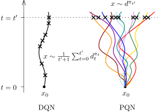
Figure 2: Sketch of Sampling Regimes in DQN and PQN

Analysis shows that when sampling online from an MDP’s true stationary distribution, off-policy instability is mitigated [76, 21]. PQN’s sampling further aids algorithmic stability by better approximating this regime in two ways: firstly, the parallelised nature of PQN means exploration policies in stochastic environments can be more greedy as the natural stochasticity in the dynamics means even a greedy policy will explore several different states in parallel. This makes PQN’s sampling closer to the online regime under the true greedy policy according to the optimal Bellman operator. Secondly, by taking multiple actions in multiple states, PQN’s sampling distribution is a good approximation of the true stationary distribution under the current policy: as time progresses, ergodic theory states that this sampling distribution converges to $d^{\pi_{t^{\prime}}}$. In contrast, sampling from a replay buffer involves sampling from an average of older stationary distributions under shifting policies from a single agent, which will be more offline and take longer to converge, as illustrated in Fig. 2.

5 Experiments

In contrast to prior work in $Q$-learning, which has focused heavily on evaluation in the Atari Learning Environment (ALE) [6], probably overfitting to this environment, we evaluate PQN on a range of single- and multi-agent environments, with PPO as the primary baseline. We summarise the memory and sample efficiency of PQN in Table 2. Due to our extensive evaluation, additional results are presented in Appendix G. All experimental results are shown as mean of 10 seeds, except in ALE where we followed a common practice of reporting 3 seeds.

5.1 Confirming Theoretical Results

DeepSea

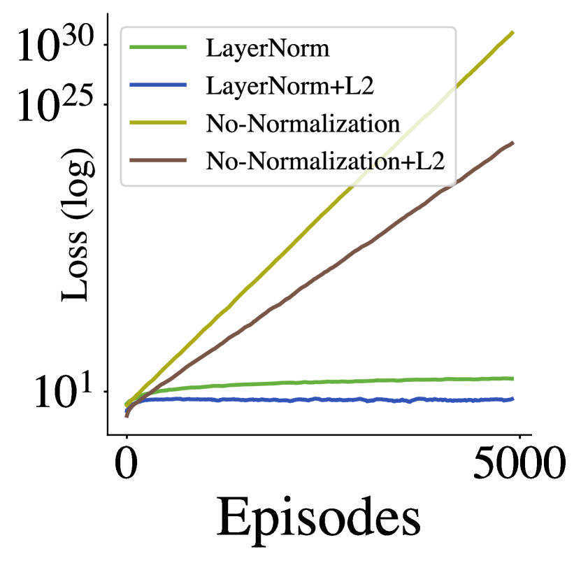
(a) Baird’s C.example

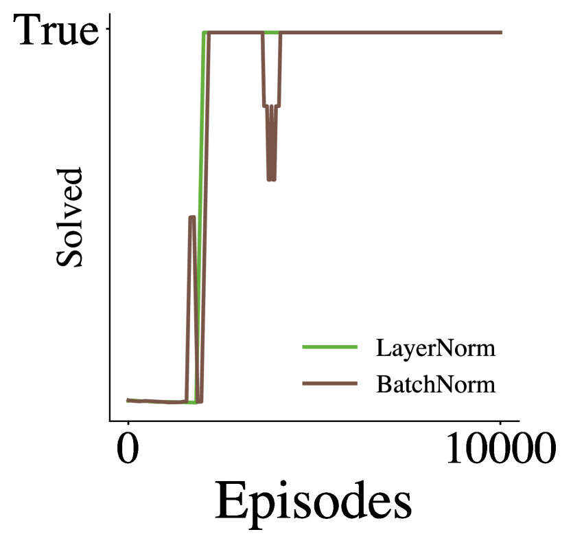
(b) DeepSea, depth 20

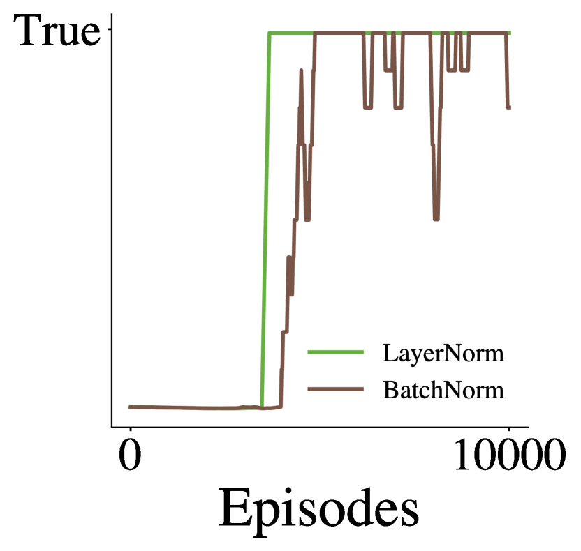
(c) DeepSea, depth 30

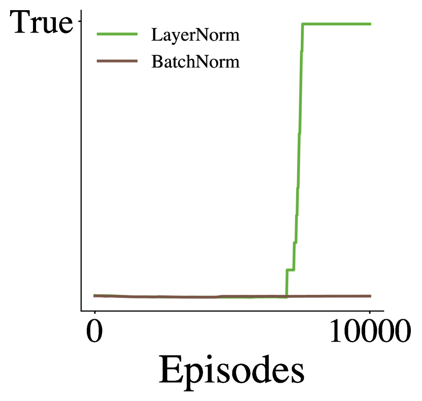
(d) DeepSea, depth 40

Figure 7: Results from theoretical analysis in Baird’s Counterexample and DeepSea.

Domains like MuJoCo where BatchNorm-based algorithm CrossQ is evaluated [9] have dense reward signal to completion and so disguise the myopic behaviour of BatchNorm our analysis uncovered in Section 3.1. More formally, these domains have a low effective horizon [40]. To confirm our analysis, we test in DeepSea, a domain where reward signal is withheld for several timesteps, meaning that a myopic agent struggles to take actions towards task completion. As seen in Fig. 7 (b)-(d) of Appendix G, when combined with LayerNorm, this simple method can solve deep veriants of DeepSea. However, even for a relatively modest batchsize of 128, when combined with BatchNorm, myopic behaviour emerges and the algorithm becomes unstable and fails to find the solution at a depth of 40.

Baird’s Counterexample

Fig. 7 (a) of Appendix G shows that together LayerNorm + $\ell_{2}$ can stabilise TD in Baird’s counterexample [4], a challenging environment that is intentionally designed to be provably divergent, even for linear function approximators. Our results show that stabilisation is mostly attributed to the introduction of LayerNorm. Moreover the degree of $\ell_{2}$-regularisation needed is small - just enough to mitigate off-policy stability due to final layer weights according to Theorem 2 - and it makes relatively little difference when used in isolation.

5.2 Atari

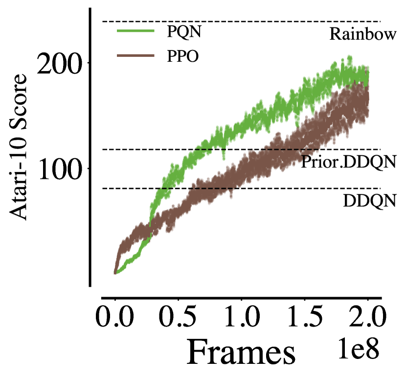
(a) Atari-10 Score

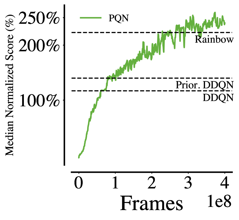
(b) Atari-57 Median

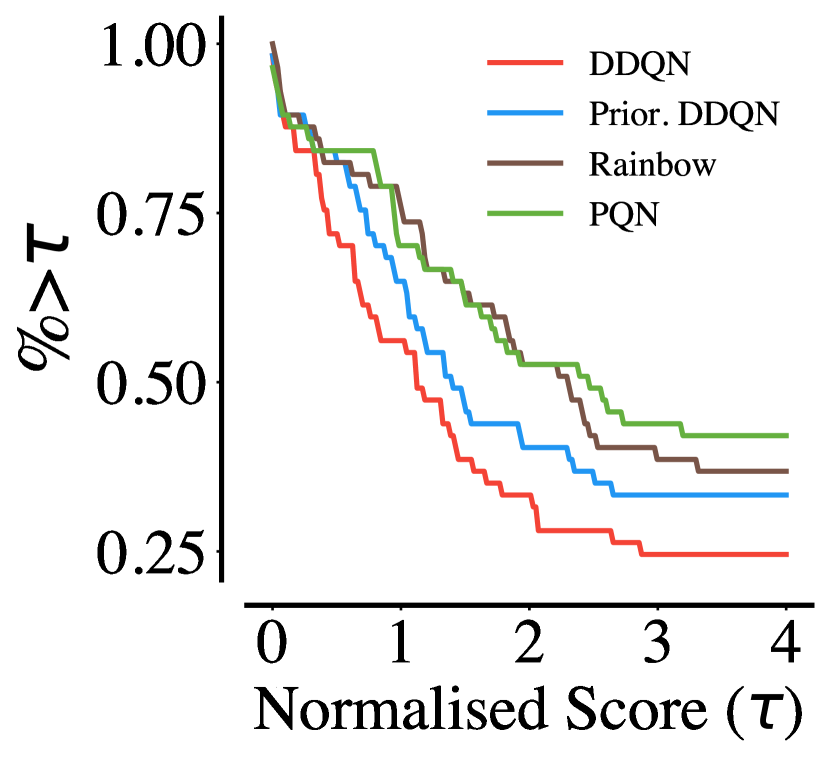
(c) Atari-57 Score Profile

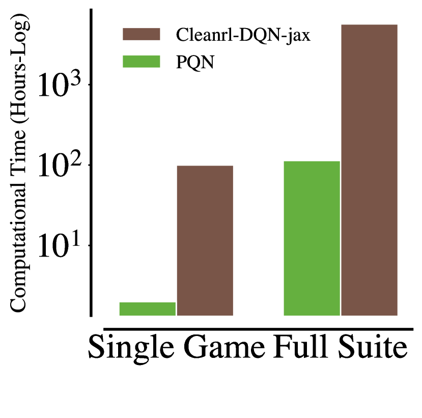
(d) Speed Comparison

Figure 3: (a) Comparison between PPO and PQN in Atari-10. (b) Median score of PQN in the full Atari suite of 57 games. (c) Percentage of games with score higher than (multiplied) human score. (d) Computational time required to run a single game and the full ALE suite for PQN and DQN implementation of CleanRL. In (c) and (d) performances of PQN are relative to training for 400M frames.

To save computational resources, we evaluate PQN against PPO in the Atari-10 suite of games from the ALE, which estimates the median across the full suite using a smaller sample of games. In Fig. 3(a) we see that PQN obtains a better Atari-10 score than PPO. Both methods beat sample efficient methods like Double-DQN and Prioritised DDQN in the same number of frames. Notably, in the same number of frames PQN performs more than 50 times fewer gradient updates than traditional DQN methods, demonstrating the significant boost in computational efficiency of our method. This, combined with vectorised sampling, results into 100x time speedup. To further test our method, we train PQN for an additional hour in the full suite of 57 Atari games. Fig. 3(d) shows the time needed to train PQN in the full Atari suite takes the same time needed to train traditional DQN methods a single game. With an additional budget of 100M frames (30 minutes of training), PQN reaches the median score of Rainbow [29]. In addition to Atari-57, in Appendix G we provide a comparative histogram of the performances of all algorithms. Notice that PQN reaches human performances in 40 of the 57 games of ALE, failing expecially in the hard-exploration games. This suggests that $\epsilon$-greedy exploration used by PQN is too simple for solving ALE, opening up a promising avenue for future research. Moreover, the lack of the replay buffer doesn’t allow to use the prioritised buffer, which can be seen as a limitation of PQN but also as a challenge for future DVRL research.

5.3 Craftax

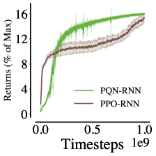
Figure 4: Craftax Score

Craftax [51] is an open-ended RL environment based on Crafter [28] and Nethack [39]. It is a challenging environment requiring solving multiple tasks to be completed. By design, Craftax is fast to run in a pure-GPU setting, but existing benchmarks are based solely on PPO. The observation size of the symbolic environment is around 8000 floats, making a pure-GPU DQN implementation with a buffer prohibitive, as it would take around 30GBs of GPU-ram. PQN on the other hand, represents a viable $Q$-learning baseline. We evaluate for 1B steps and compared PQN to PPO using both an MLP and an RNN. The RNN results are shown in Fig. 4. PQN is more sample efficient and with a RNN obtains a higher score of 16% against the 15.3% of PPO-RNN. The two methods also take a similar amount of time to train. We consider it a success to offer researchers a simple $Q$-learning alternative to PPO that can run on GPU on this challenging environment.

5.4 Multi-Agent Tasks

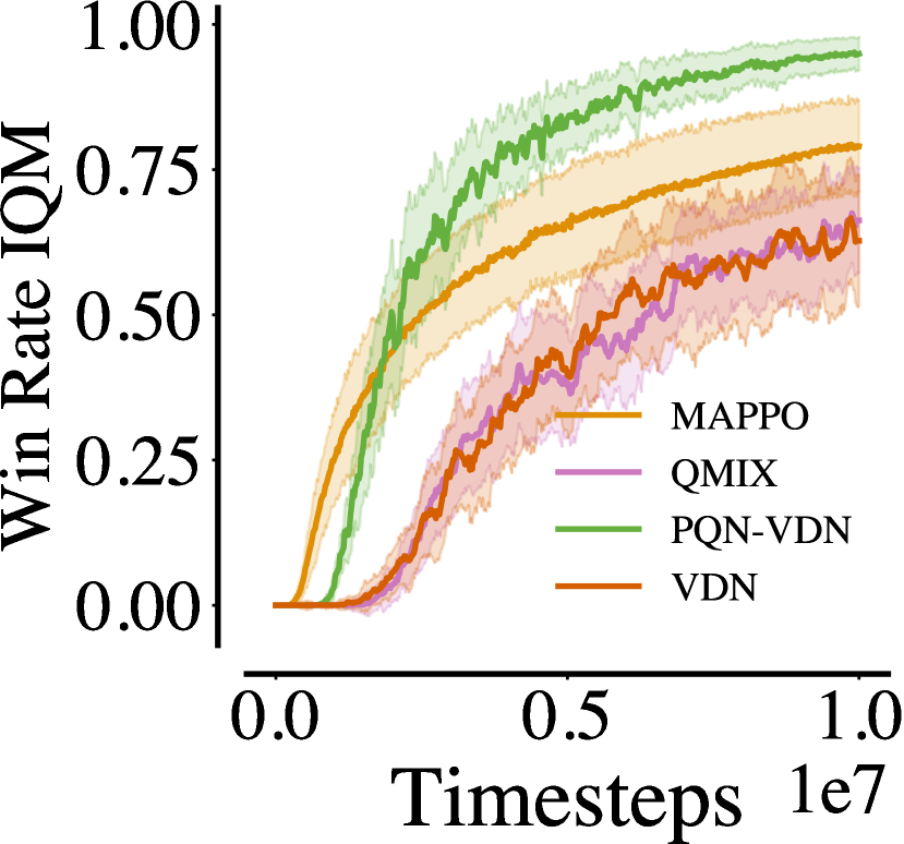
(a) Smax

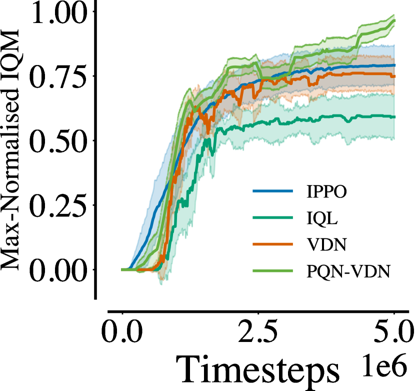
(b) Overcooked

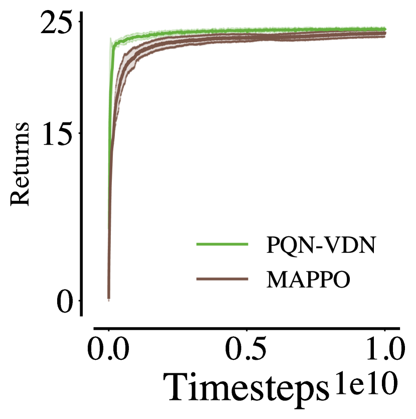
(c) Hanabi

Figure 5: Results in Multi-Agent tasks: For Smax, we report the Interquartile Mean (IQM) of the Win Rate on the 9 most popular maps. For Overcooked, we report the IQM of the returns normalized by the maximum obtained score in the classic 4 layouts. In Hanabi, we report the returns of self-play in the 2-player game.

In multi-agent problems, the size of the replay buffer can scale with the number of agents. In addition, inherent partial observably requires the use of RNNs. Moreover, credit assignment, a crucial issue in MARL, is often addressed in the literature with value-based methods [70, 60]. Thus, a memory-efficient, RNN-compatible, and fast value-based method is highly desirable in MARL research. In our experiments we learn a value decomposition network (VDN) using PQN and share parameters across all agents.

We evaluate in Hanabi [5], SMAC-SMACV2 [19, 64] in its jax-vectorised version (Smax) [63] and Overcooked [12]. Existing methods that succeed in Hanabi require a highly complex distributed system based on R2D2, using 3 GPUs in parallel, 40 CPU cores and hundreds of gigabytes of RAM [32]. By contrast, PQN does not require a replay-buffer and we vectorise the entire training loop on a single GPU while exploring on thousands of environments. Hence PQN offers a greatly simplified algorithm, which achieves SOTA scores of 24.37 in 2-player game (where MAPPO obtains 23.9) while being 4 times faster (for all the results see 4) Notably, PQN beats MAPPO obtaining a high score (above 24) in only two hours. Scores for R2D2-VDN where obtained from [32] and for MAPPO from [85].

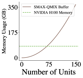
Figure 16: The buffer size scales quadratically in respect to the number of agents in SMAX.

Smax is a fast version of SMAC that can be run entirely on a single GPU. While MAPPO has obtained high scores for this benchmark, it presents a challenge for Deep $Q$-learning methods because the observation vectors scale quadratically with respect to the number of agents, as seen in Fig. 16. This means that experiments with as many as 20 agents would use up the entire memory of a typical GPU with around 10gb of RAM. We successfully run PQN-VDN on SMAX without a replay buffer and obtain higher scores than MAPPO and QMix, as seen in Fig. LABEL:fig:smax_global. Notably, the PQN implementation learns a coordination policy even in the most challenging scenarios (see Fig. LABEL:fig:smax_3s5z_vs_3s6z), in approximately 10 minutes instead of 1 hour taken by QMix.

5.5 Ablations

To examine the effectiveness of PQN’s algorithmic components, we perform the following ablations.

Regularisation:

In Fig. 6(a), we examine the effect of regularisation on performance in the Atari-10 suite. Results show LayerNorm significantly improves performance, confirming that our theoretical results of Section 3 have important empirical implications.

Varying $\lambda$:

In Fig. 6(b) we compare different values of $\lambda$ in our $Q(\lambda)$ algorithm. We find that a value of $\lambda=0.65$ performs the best by a significant margin. It significantly outperforms $\lambda=0$ (which is equal to perform 1-step update with the traditional Bellman operator) confirming that the use of $Q(\lambda)$ represents an important design choice over one-step TD.

BatchNorm:

In Fig. 6(c), we compare the performance of PQN with and without BatchNorm and note a significant difference in performance. To further investigate this, we apply BatchNorm just before the first input layer of the network, and we found the same performance as applying it BatchNorm throughout the network. This suggests that BatchNorm might help value estimation by input normalisation.

Replay Buffer:

In Fig. 6(d), we compare PQN from Algorithm 1 with a variant that maintains a replay buffer with standard size of 1M of experiences in GPU using Flashbax [74]. This version takes roughly 6x longer to train, but converges to the same final performance. The delays is likely caused by the slowness of continuously performing random access of buffer of around 30GBs, and reinforces our core message that a large memory buffer should be avoided in pure GPU training.

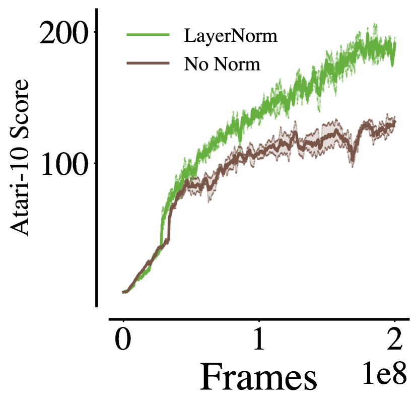
(a) LayerNorm in Atari-10

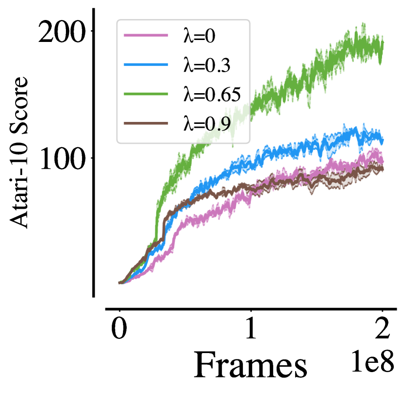
(b) $Q(\lambda)$ in Atari-10

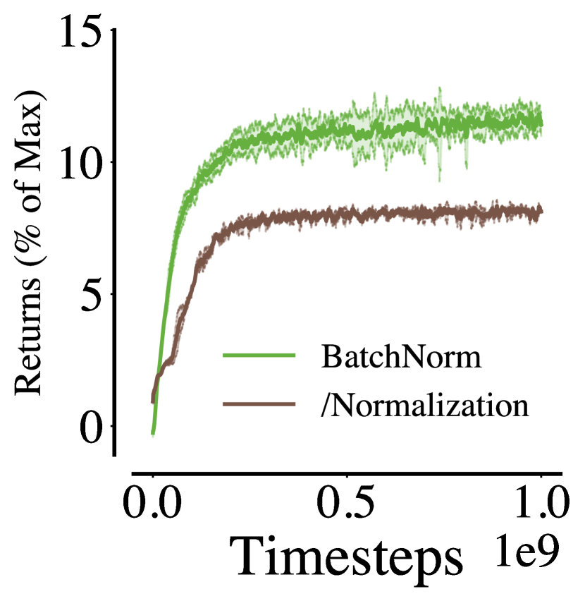
(c) BatchNorm in Craftax

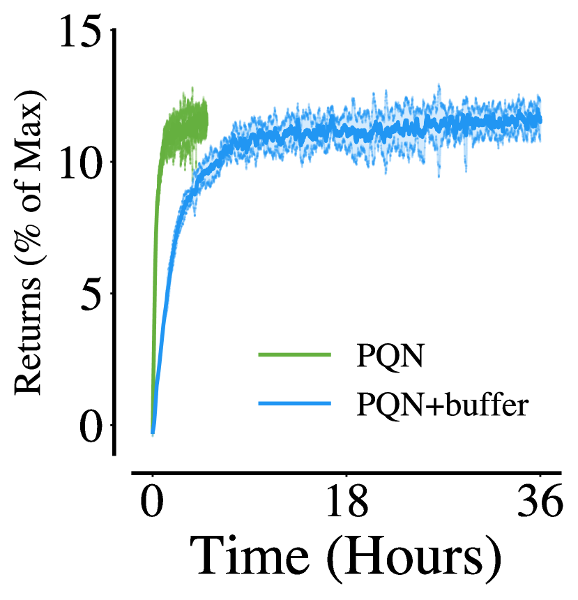
(d) Craftax with Buffer

Figure 6: Ablations confirming the importance of the different components of our method.

6 Conclusion

Table 2: Summary of Memory Saved and Speedup of PQN Compared to Baselines. The Atari speedup is relative to the traditional DQN pipeline, which runs a single environment on the CPU while training the network on GPU. Smax and Craftax speedups are relative to baselines that also run entirely on GPU but use a replay buffer. The Hanabi speed-up is relative to an R2D2 multi-threaded implementation.

	Memory Saved	Speedup
Atari	26gb	50x
Smax	10gb (up to hundreds)	6x
Hanabi	250gb	4x
Craftax	31gb	6x

We have presented the first rigorous analysis explaining the stabilising properties of LayerNorm and $\ell_{2}$ regularisation in TD methods. These results allowed us to develop PQN, a simple, stable and efficient regularised $Q$-learning algorithm without the need for target networks or a replay buffer. PQN exploits vectorised computation to achieve excellent performance across an extensive empirical evaluation with a significant boost in computational efficiency. By saving the memory occupied by the replay buffer, PQN paves the way for a generation of powerful but stable algorithms that exploit end-to-end GPU vectorised deep RL.

Appendix A Broader Impact

Our theoretical results aid researchers in designing stable algorithms. Unintended divergence of algorithms represents a serious risk for deployment of RL, which our results aim to reduce. Our PQN algorithm represents a significant simplification of existing methods achieving state-of-the-art performance with a speedup in computational efficiency. PQN contributes to the wider trend of more powerful ML algorithms becoming more broadly accessible. This has the potential for both positive and negative societal impacts, a full review of which is beyond the scope of this paper.

Appendix B Related Work

B.1 Regularisation

A key ingredient for stabilising TD is the introduction of regularisation, either into the value function or into the TD vector. In this paper, we study the following regularisation techniques:

$\ell_{p}$-Norms

For a vector $v\in\mathbb{R}^{k}$ we denote the $\ell_{2}$-norm as $\lVert v\rVert\coloneqq\sqrt{\sum_{i=0}^{k-1}v_{i}^{2}}$ and the $\ell_{\infty}$-norm as $\lVert v\rVert_{\textrm{max}}\coloneqq\max_{i}\lvert v_{i}\rvert$. One of the simplest forms of regularisation adds a $\ell_{2}$-norm term $\eta\lVert\phi_{0}-\phi\rVert^{2}$ to a minimisation objective where and $\eta\geq 0$ is a scalar that controls the degree of regularisation. Intuitively, $L_{2}$ regularisation penalises updates to the parameter $\phi$ that stray too far from $\phi_{0}$. As TD learning is not a gradient of any objective, the derivative of the term is added to parameter update directly: $\delta_{\ell_{2}}(\phi,x)=\delta(\phi,x)+\eta(\phi_{0}-\phi)$.

BatchNorm

First introduced by Ioffe and Szegedy [35], for a function $f:\mathcal{X}\rightarrow\mathbb{R}^{k}$ the $N$-sample BatchNorm operator is defined element-wise on each dimension $i\in[1:k]$ as:

$$\textrm{BatchNorm}_{N}^{i}[f](x)\coloneqq \frac{f^{i}(x)-\hat{\mu}^{i}_{N}\left[f\right]}{\hat{\sigma}^{i}_{N}[f]},$$ (9)

where $\hat{\mu}_{N}^{i}\left[f\right]$ and $\hat{\sigma}^{i}_{N}[f]$ are the element-wise empirical mean and standard deviation under the batch of data $\mathcal{D}_{N}$:

$$\hat{\mu}_{N}^{i}\left[f\right]\coloneqq\frac{1}{N}\sum_{j=0}^{N-1}f^{i}(x_{j}),\quad\hat{\sigma}_{N}^{i}[f]\coloneqq\sqrt{\frac{1}{N}\sum_{j=0}^{N-1}(f^{i}(x_{j})-\hat{\mu}^{i}_{N}\left[f\right])^{2}+\epsilon},$$ (10)

and $\epsilon>0$ is a small constant added to the variance for numerical stability.

LayerNorm

As an alternative to BatchNorm, Ba et al. [2] introduced layer normalisation, which replaces the batch mean and variance with the element-wise mean and expectation across a vector. Formally, for a function $f:\mathcal{X}\rightarrow\mathbb{R}^{k}$ LayerNorm is defined element-wise as:

$$\textrm{LayerNorm}^{i}[f](x)\coloneqq \frac{1}{\sqrt{k}}\cdot\frac{f^{i}(x)-\hat{\mu}\left[f\right](x)}{\hat{\sigma}[f](x)},$$ (11)

where $\hat{\mu}\left[f\right](x)$ and $\hat{\sigma}[f](x)$ are the element-wise empirical mean and standard deviation of the output $f(x)$:

$$\hat{\mu}\left[f\right](x)\coloneqq\frac{1}{k}\sum_{i=0}^{k-1}f^{i}(x),\quad\hat{\sigma}[f](x)\coloneqq\sqrt{\frac{1}{k}\sum_{i=0}^{k-1}(f^{i}(x)-\hat{\mu}\left[f\right](x))^{2}+\epsilon},$$ (12)

and $\epsilon>0$ is a small constant added to the variance for numerical stability. Compared to BatchNorm, LayerNorm is simpler to implement and does not require memory or estimation of the running batch averages.

B.2 Parallelisation of $Q$-learning

Existing attempts to parallelise $Q$-learning adopt a distributed architecture, where a separate process continually trains the agent and sampling occurs in parallel threads which contain a delayed copy of its parameters [31, 36, 3, 30]. On the contrary, PQN samples and trains in the same process, enabling end-to-end single GPU training. While distributed methods can benefit from a separate process that continuously train the network, PQN is easier to implement, doesn’t introduce time-lags between the learning agent and the exploratory policy. Moreover, PQN can be optimised to be sample efficient other than fast, while distributed system usually ignore sample efficiency.

Mnih et al. [54] propose asynchronous $Q$-learning, a parallelised version of $Q$-learning which performs updates of a centralised network asynchronously without using a replay buffer. Compared to PQN, asynchronous $Q$-learning still use target networks and accumulates gradients over many timesteps to update the network. To our knowledge, we are the first to unlock the potential of a truly asynchronous parallelised deep $Q$-learning algorithm without a replay buffer, target networks or accumulated gradients.

B.3 Regularisation in RL

CrossQ is a recently developed off-policy algorithm based on SAC that removes target networks and introduces BatchNorm into the critic [9]. CrossQ demonstrates impressive performance when evaluated across a suite of MuJoCo domain with high sample and computational efficiency, however no analysis is provided explaining its stability properties or what effect introducing BatchNorm has. To develop PQN, we perform a rigorous analysis of both BatchNorm and LayerNorm in TD.

The benefits of regularisation has also been reported in other areas of the RL literature. Lyle et al. [47, 48] investigate plasticity loss in off-policy RL, a phenomenon where neural networks lose their ability to fit a new target functions throughout training. They propose LayerNorm [47] and LayerNorm with $\ell_{2}$ regularisation [48], as a solution to this problem, and show improved performance on the Atari Learning Environment, but they also use other methods of stabilisation, such as target networks, that we explicitly remove. There is no formal analysis to explain these results.

B.4 Parallelised Environments in Distributed Methods

Li et al. [43] explore the use of vectorised environments in distributed systems. Specifically, their algorithm parallel $Q$-learning (PQL) uses Isaac Gym to collect trajectories from thousands of parallel environments, significantly speeding up the training of a DDPG agent. However, PQL introduces additional complexity by incorporating a concurrent training process for the policy network with its own buffer, and requires multiple GPUs to run smoothly. The authors observe that when sampling is fast, the replay buffer is frequently overwritten. Therefore they propose using enormous learning batches (up to 16834) to maximise the use of collected experiences, which is computationally expensive and can affect the generalisation abilities of the trained network, since the noise introduced by smaller batches is lost [37, 55]. Empirically, they also show that increasing the size of the replay buffer does not lead to better performance. As we discuss in Section 4.1, these findings support our intuition it is more effective to use the collected trajectories directly for learning rather than storing them in a buffer when using many parallel environments.

B.5 Multi-Step $Q$-learning

The concept of n-step returns in reinforcement learning extends the traditional one-step update to consider rewards over multiple future steps. The $n$-step return for a state-action pair (s, a) is defined as the cumulative reward over the next n steps plus the discounted value of the state reached after n steps. Several variations of n-step $Q$-learning have been proposed to enhance learning efficiency and stability. Peng and Williams [58] introduced a variation known as Q($\lambda$), which integrates eligibility traces to account for multiple time steps while maintaining the off-policy nature of $Q$-learning. Replay buffers are difficult to combine with $Q(\lambda)$. Recent methods have tried to reconcile $\lambda$-returns with the experience buffer [16] most notably in TD3 [38].

B.6 Multi-Agent Deep Q Learning

$Q$-learning methods are a popular choice for multi-agent RL (MARL), especially in the purely cooperative centralised training with decentralised execution (CTDE) setting [22, 45]. In CTDE, global information is made available at training time, but not at test time. Many of these methods develop approaches to combine individual utility functions into a joint estimate of the Q function: Son et al. [67] introduce the individual-global-max (IGM) principle to describe when a centralised Q function can be computed from individual utility functions in a decentralised fashion; Value Decomposition Networks (VDN)  [69] combines individual value estimates by summing them, and QMIX [61] learns a hypernetwork with positive weights to ensure monotonicity. All these methods can be combined with PQN, which parallises the learning process.

IPPO [18] and MAPPO [86] use vectorised environments, adapting a single-agent method for use in multi-agent RL. These are both on-policy actor-critic based methods based on PPO.

Appendix C Analysis of TD

In this paper, our proofs expand on Fellows et al. [21], who introduce a framework to analyse general nonlinear TD methods, showing that for function approximators for which the Jacobian $\nabla_{\phi}\delta(\phi)$ is defined almost everywhere, stability is determined by the eigenvalues of the single step path-mean TD Jacobian, defined as: $\bar{J}_{\textrm{TD}}(\phi,\phi^{\star})\coloneqq\int_{0}^{1}\nabla_{\phi}\delta(\phi-l(\phi-\phi^{\star}))dl$. Intuitively, a path-mean Jacobian is the average of all Jacobians along the line joining $\phi$ to the TD fixed point $\phi^{\star}$. The path-mean Jacobian can be used to show that stability of TD is guaranteed if the following stability criterion is satisfied [21, Theorem 1]:

TD Stability Criterion

For every $\phi\in\phi$, $\bar{J}_{\textnormal{{TD}}}(\phi,\phi^{\star})$ has strictly negative eigenvalues. Analysing the Jacobian:

$$J_{\textrm{TD}}(\phi)=\nabla_{\phi}\delta(\phi) =\gamma\mathbb{E}_{\varsigma\sim P_{\varsigma}}\left[\nabla_{\phi}Q_{\phi}(x^{\prime})\nabla_{\phi}Q_{\phi}(x)^{\top}\right]-\mathbb{E}_{\varsigma\sim P_{\varsigma}}\left[\nabla_{\phi}Q_{\phi}(x)\nabla_{\phi}Q_{\phi}(x)^{\top}\right],$$ (13)

$$\qquad+\mathbb{E}_{\varsigma\sim P_{\varsigma}}\left[(r+\gamma Q_{\phi}(x^{\prime})-Q_{\phi}(x))\nabla_{\phi}^{2}Q_{\phi}(x)\right],$$ (14)

the TD stability criterion is not automatically satisfied in general TD algorithms due to the two sources of instability identified in Section 2.4 [21, Section 4.1]. Firstly, the matrix on Line 13 is negative definite if

$$\gamma v^{\top}\mathbb{E}_{\varsigma\sim P_{\varsigma}}\left[\nabla_{\phi}Q_{\phi}(x^{\prime})\nabla_{\phi}Q_{\phi}(x)^{\top}\right]v<v^{\top}\mathbb{E}_{x\sim d^{\mu}}\left[\nabla_{\phi}Q_{\phi}(x)\nabla_{\phi}Q_{\phi}(x)^{\top}\right]v,$$ (15)

for any test vector $v$ due to off-policy instability. Secondly, the matrix on Line 14 is negative definite if

$$\mathbb{E}_{\varsigma\sim P_{\varsigma}}\left[(r+\gamma Q_{\phi}(x^{\prime})-Q_{\phi}(x))v^{\top}\nabla_{\phi}^{2}Q_{\phi}(x)v\right]<0,$$ (16)

for any test vector $v$ due to nonlinear instability. Moreover, if the path-mean Jacobian has any positive eigenvalues then it can be shown that there exist initial parameter values such that TD is provably divergent.

Appendix D Proofs

D.1 Theorem 1- Analysis of BatchNorm

Theorem 1.

Under 1, using the BatchNorm $Q$-function defined in Eq. 6 $\lim_{N\rightarrow\infty}\mathbb{E}_{x_{t}\sim d^{\mu}}\left[\mathcal{B}\left[Q_{\phi}\right](x_{t})\right]=\mathbb{E}_{r\sim P_{R}(x_{t}),x_{t}\sim d^{\mu}}\left[r\right]$ almost surely.

Proof.

We first prove $\lim_{N\rightarrow\infty}\mathbb{E}_{x^{\prime}\sim P^{\mu,\pi}}\left[\textrm{BatchNorm}_{N}[f](x^{\prime})\right]$ element-wise. Under the Lebesgue dominated convergence theorem:

$$\lim_{N\rightarrow\infty} \mathbb{E}_{x^{\prime}\sim P^{\mu,\pi}}\left[\textrm{BatchNorm}^{i}_{N}[f](x^{\prime})\right],$$ (17)

$$=\mathbb{E}_{x^{\prime}\sim P^{\mu,\pi}}\left[\lim_{N\rightarrow\infty}\textrm{BatchNorm}^{i}_{N}[f](x^{\prime})\right],$$ (18)

$$=\mathbb{E}_{x^{\prime}\sim P^{\mu,\pi}}\left[\lim_{N\rightarrow\infty}\frac{f(x^{\prime})-\hat{\mu}^{i}_{N}[f]}{\hat{\sigma}^{i}_{N}[f]}\right].$$ (19)

Under 1, we can apply the strong law of large numbers (see Williams [83, Theorem 14.5] for the i.i.d. case or Gilks et al. [24, Theorem 4.3] for the Markov chain case): $\lim_{N\rightarrow\infty}\hat{\mu}_{N}^{i}\left[f\right]=\mathbb{E}_{x^{\prime}\sim P^{\mu,\pi}}\left[f^{i}\right]$ and $\lim_{N\rightarrow\infty}\hat{\sigma}^{i}_{N}[f]=\sqrt{\mathbb{V}_{x^{\prime}\sim P^{\mu,\pi}}\left[f^{i}(x^{\prime})\right]+\epsilon}$ almost surely, hence:

$$\lim_{N\rightarrow\infty} \mathbb{E}_{x^{\prime}\sim P^{\mu,\pi}}\left[\textnormal{{BatchNorm}}_{N}^{i}[f](x^{\prime})\right]$$ (20)

$$=\mathbb{E}_{x^{\prime}\sim P^{\mu,\pi}}\left[\frac{f^{i}(x^{\prime})-\mathbb{E}_{x^{\prime}\sim P^{\mu,\pi}}\left[f^{i}(x^{\prime})\right]}{\sqrt{\mathbb{V}_{x^{\prime}\sim P^{\mu,\pi}}\left[f^{i}(x^{\prime})\right]+\epsilon}}\right],$$ (21)

$$=\frac{\mathbb{E}_{x^{\prime}\sim P^{\mu,\pi}}\left[f^{i}(x^{\prime})\right]-\mathbb{E}_{x^{\prime}\sim P^{\mu,\pi}}\left[f^{i}(x^{\prime})\right]}{\sqrt{\mathbb{V}_{x^{\prime}\sim P^{\mu,\pi}}\left[f^{i}(x^{\prime})\right]+\epsilon}},$$ (22)

$$=0.$$ (23)

Taking the limit of the expected Bellman operator:

$$\lim_{N\rightarrow\infty}\mathbb{E}_{x_{t}\sim d^{\mu}}\left[\mathcal{B}^{\pi}\left[Q_{\phi}\right](x_{t})\right] =\lim_{N\rightarrow\infty}\mathbb{E}_{x_{t}\sim d^{\mu}}\left[\mathbb{E}_{x_{t+1}\sim P_{X}^{\pi}(x_{t}),r_{t}\sim P(x_{t})}\left[r_{t}+\gamma Q^{\pi}(x_{t+1})\right]\right],$$ (24)

$$=\mathbb{E}_{r\sim P_{R}(x_{t}),x_{t}\sim d^{\mu}}\left[r\right]+\lim_{N\rightarrow\infty}\gamma\mathbb{E}_{x_{t+1}\sim P^{\mu,\pi}}\left[Q^{\pi}(x_{t+1})\right].$$ (25)

Now,

$$\lim_{N\rightarrow\infty}\gamma\mathbb{E}_{x_{t+1}\sim P^{\mu,\pi}}\left[Q^{\pi}(x_{t+1})\right] =\gamma\mathbb{E}_{x_{t+1}\sim P^{\mu,\pi}}\left[\lim_{N\rightarrow\infty}Q^{\pi}(x_{t+1})\right],$$ (26)

$$=\gamma w^{\top}\mathbb{E}_{x_{t+1}\sim P^{\mu,\pi}}\left[\lim_{N\rightarrow\infty}\textrm{BatchNorm}_{N}[f](x_{t+1})\right],$$ (27)

$$=0,$$ (28)

hence:

$$\lim_{N\rightarrow\infty}\mathbb{E}_{x_{t}\sim d^{\mu}}\left[\mathcal{B}\left[Q_{\phi}\right](x_{t})\right]=\mathbb{E}_{r\sim P_{R}(x_{t}),x_{t}\sim d^{\mu}}\left[r\right],\quad a.s.$$ (29)

∎

D.2 Theorem 2 - Mitigating Off-Policy Instability

Theorem 2.

Under 2, using the LayerNorm $Q$-function defined in Eq. 7:

$$\frac{\gamma v^{\top}\nabla_{\phi}Q_{\phi}(x^{\prime})\nabla_{\phi}Q_{\phi}(x)^{\top}v-(v^{\top}\nabla_{\phi}Q_{\phi}(x))^{2}}{\lVert v\rVert^{2}}\leq\left(\frac{\gamma}{2}\right)^{2}+\mathcal{O}\left(\frac{1}{\sqrt{k}}\right),$$ (30)

almost surely for any test vector $v\in\Phi$ and any state-action transition pair $x,x^{\prime}\in\mathcal{X}$.

Proof.

We start by writing $M$ in terms of its row vectors:

$$M=\begin{bmatrix}\begin{array}[]{@{\protect\rotvert\;}c@{\;\protect\rotvert}}\rotatebox[origin={c}]{90.0}{$|$}\;\lx@intercol\hfil m_{0}^{T}\hfil\;\rotatebox[origin={c}]{90.0}{$|$}\\ \rotatebox[origin={c}]{90.0}{$|$}\;\lx@intercol\hfil m_{1}^{\top}\hfil\;\rotatebox[origin={c}]{90.0}{$|$}\\ \lx@intercol\hfil\vdots\hfil\\ \rotatebox[origin={c}]{90.0}{$|$}\;\lx@intercol\hfil m_{k-1}^{\top}\hfil\;\rotatebox[origin={c}]{90.0}{$|$}\end{array}\end{bmatrix}.$$ (31)

and splitting the test vector into the corresponding $k+1$ sub-vectors:

$$v^{\top}=[v_{w}^{T},v_{m_{0}}^{\top},v_{m_{1}}^{\top},\cdots v_{m_{k-1}}^{\top}],$$ (32)

where $v_{w}$ is a vector with the same dimension as the final weight vector $w$ and each $v_{m_{i}}\in\mathbb{R}^{n}$ has the same dimension as $x$. Under this notation, we split the left hand side of Eq. 30 into two terms, one determining the stability of the final layer weights and one for the matrix vectors:

$$\frac{\gamma v^{\top}\nabla_{\phi}Q_{\phi}(x^{\prime})\nabla_{\phi}Q_{\phi}(x)^{\top}v-(v^{\top}\nabla_{\phi}Q_{\phi}(x))^{2}}{\lVert v\rVert^{2}}$$ (33)

$$\quad=\frac{\gamma v_{w}^{\top}\nabla_{w}Q_{\phi}(x^{\prime})\nabla_{w}Q_{\phi}(x)^{\top}v_{w}-(v_{w}^{\top}\nabla_{w}Q_{\phi}(x))^{2}}{\lVert v\rVert^{2}}$$ (34)

$$\qquad+\frac{\sum_{i=0}^{k-1}\left(\gamma v_{m_{i}}^{\top}\nabla_{m_{i}}Q_{\phi}(x^{\prime})\nabla_{m_{i}}Q_{\phi}(x)^{\top}v_{m_{i}}-v_{m_{i}}^{\top}\nabla_{m_{i}}Q_{\phi}(x)\nabla_{m_{i}}Q_{\phi}(x)^{\top}v_{m_{i}}\right)}{\lvert v\rVert^{2}}.$$ (35)

Applying Lemmas 1 and 2, we bound both terms to yield our desired result:

$$\frac{\gamma v^{\top}\nabla_{\phi}Q_{\phi}(x^{\prime})\nabla_{\phi}Q_{\phi}(x)^{\top}v-(v^{\top}\nabla_{\phi}Q_{\phi}(x))^{2}}{\lVert v\rVert^{2}}\leq\left(\frac{\gamma}{2}\right)^{2}+\mathcal{O}\left(\frac{1}{\sqrt{k}}\right),$$ (36)

almost surely. ∎

Lemma 1.

Under 2, using the LayerNorm critic in Eq. 7:

$$\frac{\gamma v_{w}^{\top}\nabla_{w}Q_{\phi}(x^{\prime})\nabla_{w}Q_{\phi}(x)^{\top}v_{w}-(v_{w}^{\top}\nabla_{w}Q_{\phi}(x))^{2}}{\lVert v\rVert^{2}}\leq\left(\frac{\gamma}{2}\right)^{2}.$$ (37)

Proof.

Taking derivatives of the critic with respect to the final layer weights $w$ yields:

$$\nabla_{w}Q_{\phi}(x) =\textrm{ReLU}\circ\textrm{LayerNorm}\left[Mx\right],$$ (38)

$$=\mathbb{I}(Wx)\odot\textrm{LayerNorm}\left[Mx\right].$$ (39)

We then bound $v_{w}^{\top}\nabla_{w}Q_{\phi}(x^{\prime})\nabla_{w}Q_{\phi}(x)^{\top}v_{w}$ as:

$$v_{w}^{\top}\nabla_{w}Q_{\phi}(x^{\prime})\nabla_{w}Q_{\phi}(x)^{\top}v_{w} \leq\lVert v_{w}\rVert\lVert\nabla_{w}Q_{\phi}(x^{\prime})\rVert\lvert\nabla_{w}Q_{\phi}(x)^{\top}v_{w}\rvert.$$ (40)

Now, bounding the derivative $\nabla_{w}Q_{\phi}(x)$:

$$\lVert\nabla_{w}Q_{\phi}(x)\rVert =\left\lVert\mathbb{I}(Wx)\odot\textrm{LayerNorm}\left[Mx\right]\right\rVert,$$ (41)

$$\leq\lVert\mathbb{I}(Wx)\rVert_{\textrm{max}}\cdot\left\lVert\textrm{LayerNorm}\left[Mx\right]\right\rVert,$$ (42)

$$=\left\lVert\textrm{LayerNorm}\left[Mx\right]\right\rVert.$$ (43)

Substituting for $\lVert\textnormal{{LayerNorm}}[Mx]\rVert\leq 1$ from Proposition 1 yields:

$$\lVert\nabla_{w}Q_{\phi}(x)\rVert \leq 1,$$ (44)

hence:

$$v_{w}^{\top}\nabla_{w}Q_{\phi}(x^{\prime})\nabla_{w}Q_{\phi}(x)^{\top}v_{w} \leq\lVert v_{w}\rVert\lvert\nabla_{w}Q_{\phi}(x)^{\top}v_{w}\rvert,$$ (45)

Applying Inequality 45 to the left hand side of Inequality 37 and defining $\eta\coloneqq\lvert\nabla_{w}Q_{\phi}(x)^{\top}v_{w}\rvert$ yields:

$$\gamma v_{w}^{\top}\nabla_{w}Q_{\phi}(x^{\prime})\nabla_{w}Q_{\phi}(x)^{\top}v_{w}-(v_{w}^{\top}\nabla_{w}Q_{\phi}(x))^{2} \leq\gamma w_{\textrm{max}}\lvert\nabla_{w}Q_{\phi}(x)^{\top}v_{w}\rvert-\lvert\nabla_{w}Q_{\phi}(x)^{\top}v_{w}\rvert^{2},$$ (46)

$$=\gamma\lVert v_{w}\rVert\eta-\eta^{2},$$ (47)

$$\leq\max_{\eta}\left(\gamma\lVert v_{w}\rVert\eta-\eta^{2}\right).$$ (48)

Our desired result follows from the fact that the function $\gamma\lVert v_{w}\rVert\eta-\eta^{2}$ is maximised at $\eta=\frac{\gamma\lVert v_{w}\rVert}{2}$, hence:

$$\gamma v_{w}^{\top}\nabla_{w}Q_{\phi}(x^{\prime})\nabla_{w}Q_{\phi}(x)^{\top}v_{w}-(v_{w}^{\top}\nabla_{w}Q_{\phi}(x))^{2}\leq\frac{\gamma^{2}\lVert v_{w}\rVert}{2}-\left(\frac{\gamma\lVert v_{w}\rVert}{2}\right)^{2} =\left(\frac{\gamma\lVert v_{w}\rVert}{2}\right)^{2},$$ (49)

$$\implies\frac{\gamma v_{w}^{\top}\nabla_{w}Q_{\phi}(x^{\prime})\nabla_{w}Q_{\phi}(x)^{\top}v_{w}-(v_{w}^{\top}\nabla_{w}Q_{\phi}(x))^{2}}{\lVert v\rVert^{2}}\leq\left(\frac{\gamma\lVert v_{w}\rVert}{2\lVert v\rVert}\right)^{2} \leq\left(\frac{\gamma}{2}\right)^{2}.$$ (50)

∎

Lemma 2.

Under 2,

$$\frac{1}{\lVert v\rVert^{2}}\sum_{i=0}^{k-1}\big{(} \gamma v_{m_{i}}^{\top}\nabla_{m_{i}}Q_{\phi}(x^{\prime})\nabla_{m_{i}}Q_{\phi}(x)^{\top}v_{m_{i}}$$ (51)

$$-v_{m_{i}}^{\top}\nabla_{m_{i}}Q_{\phi}(x)\nabla_{m_{i}}Q_{\phi}(x)^{\top}v_{m_{i}}\big{)}=\mathcal{O}\left(\frac{1}{\sqrt{k}}\right),$$ (52)

almost surely.

Proof.

Writing the critic as:

$$Q_{\phi}(x)=\sum_{j=0}^{k-1}w_{j}\textrm{ReLU}\circ\textrm{LayerNorm}_{j}\left[Mx\right],$$ (53)

we apply the chain rule to find the derivative of the critic with respect to each row vector:

$$\nabla_{m_{i}}Q_{\phi}(x) =\sum_{j=0}^{k-1}w_{j}\partial\textrm{ReLU}\circ\textrm{LayerNorm}_{j}\left[Mx\right]\nabla_{m_{i}}\textrm{LayerNorm}_{j}\left[Mx\right],$$ (54)

$$=\sum_{j=0}^{k-1}w_{j}\mathbbm{1}\left(\textrm{LayerNorm}_{j}\left[Mx\right]>0\right)\nabla_{m_{i}}\textrm{LayerNorm}_{j}\left[Mx\right],$$ (55)

$$\implies\nabla_{m_{i}}Q_{\phi}(x)^{\top}v_{m_{i}} =\sum_{j=0}^{k-1}w_{j}\mathbbm{1}\left(\textrm{LayerNorm}_{j}\left[Mx\right]>0\right)\nabla_{m_{i}}\textrm{LayerNorm}_{j}\left[Mx\right]^{\top}v_{m_{i}}.$$ (56)

Applying Lemma 3 to find $\nabla_{m_{i}}\textrm{LayerNorm}_{j}\left[Mx\right]^{\top}v_{m_{i}}$:

$$\nabla_{m_{i}}Q_{\phi}(x)^{\top}v_{m_{i}} =\sum_{j=0}^{k-1}w_{j}\mathbbm{1}\left(\textrm{LayerNorm}_{j}\left[Mx\right]>0\right)\nabla_{m_{i}}\textrm{LayerNorm}_{j}\left[Mx\right]^{\top}v_{m_{i}},$$ (57)

$$=\frac{1}{\sqrt{k}}\sum_{j=0}^{k-1}\left(w_{j}\mathbbm{1}\left(\textrm{LayerNorm}_{j}\left[Mx\right]>0\right)\mathbbm{1}(i=j)\frac{x^{\top}v_{m_{i}}}{\hat{\sigma}\left[Mx\right]}+\mathcal{O}\left(\frac{1}{k}\right)\right),$$ (58)

$$=\frac{1}{\sqrt{k}}\left(w_{i}\mathbbm{1}\left(\textrm{LayerNorm}_{i}\left[Mx\right]>0\right)\frac{x^{\top}v_{m_{i}}}{\hat{\sigma}\left[Mx\right]}+\mathcal{O}\left(1\right)\right).$$ (59)

Now, as $\lVert\phi\rVert<\infty$ almost surely under 2, $w_{i}<\infty$ almost surely, hence:

$$\nabla_{m_{i}}Q_{\phi}(x)^{\top}v_{m_{i}}=\mathcal{O}\left(\frac{1}{\sqrt{k}}\right).$$ (60)

Finally, we substitute into the left hand side of Eq. 52 to yield our desired result:

$$\frac{1}{\lVert v\rVert^{2}}\sum_{i=0}^{k-1}\left(\gamma v_{m_{i}}^{\top}\nabla_{m_{i}}Q_{\phi}(x^{\prime})\nabla_{m_{i}}Q_{\phi}(x)^{\top}v_{m_{i}}-v_{m_{i}}^{\top}\nabla_{m_{i}}Q_{\phi}(x)\nabla_{m_{i}}Q_{\phi}(x)^{\top}v_{m_{i}}\right),$$ (61)

$$=\mathcal{O}\left(\frac{1}{\sqrt{k}}\right)\frac{1}{\lVert v\rVert^{2}}\sum_{i=0}^{k-1}\lVert v_{m_{i}}\rVert^{2}\left(\gamma\mathcal{O}\left(1\right)-\mathcal{O}\left(1\right)\right),$$ (62)

$$=\mathcal{O}\left(\frac{1}{\sqrt{k}}\right)\frac{1}{\lVert v\rVert^{2}}\sum_{i=0}^{k-1}\lVert v_{m_{i}}\rVert^{2},$$ (63)

$$=\mathcal{O}\left(\frac{1}{\sqrt{k}}\right)\frac{\lVert v_{m}\rVert^{2}}{\lVert v\rVert^{2}}=\mathcal{O}\left(\frac{1}{\sqrt{k}}\right).$$ (64)

∎

Proposition 1.

For any $f:\mathcal{X}\rightarrow\mathbb{R}^{k}$:

$$\lVert\textnormal{{LayerNorm}}[f(x)]\rVert\leq 1.$$ (65)

Proof.

Our result follows from the definition of LayerNorm:

$$\lVert\textnormal{{LayerNorm}}[f_{\phi}(x)]\rVert =\frac{1}{\sqrt{k}}\frac{\lVert f(x)-\hat{\mu}\left[f\right](x)\rVert}{\hat{\sigma}[f](x)},$$ (66)

$$=\frac{\sqrt{\frac{1}{k}\sum_{i=0}^{k-1}\left(f^{i}(x)-\hat{\mu}\left[f\right](x)\right)^{2}}}{\hat{\sigma}[f](x)},$$ (67)

$$\leq\frac{\sqrt{\frac{1}{k}\sum_{i=0}^{k-1}\left(f^{i}(x)-\hat{\mu}\left[f\right](x)\right)^{2}+\epsilon}}{\hat{\sigma}[f](x)},$$ (68)

$$=\frac{\hat{\sigma}[f](x)}{\hat{\sigma}[f](x)},$$ (69)

$$=1,$$ (70)

as required. ∎

Lemma 3.

$$\nabla_{m_{i}}\textnormal{{LayerNorm}}_{j}\left[Mx\right]^{\top}v_{m_{i}}=\frac{1}{\sqrt{k}}\left(\mathbbm{1}(i=j)\frac{x^{\top}v_{m_{i}}}{\hat{\sigma}\left[Mx\right]}+\mathcal{O}\left(\frac{1}{k}\right)\right).$$ (71)

Proof.

Taking the derivative of $\textrm{LayerNorm}_{j}\left[Mx\right]$ with respect to $m_{i}$ yields:

$$\nabla_{m_{i}}\textrm{LayerNorm}_{j}\left[Mx\right]=\frac{1}{\sqrt{k}}\left(\left(\mathbbm{1}(i=j)-\frac{1}{k}\right)\frac{x}{\hat{\sigma}\left[Mx\right]}-\frac{m_{i}^{\top}x-\hat{\mu}\left[Mx\right]}{\hat{\sigma}\left[Mx\right]^{2}}\nabla_{m_{i}}\hat{\sigma}\left[Mx\right]\right),$$ (72)

We find $\nabla_{m_{i}}\hat{\sigma}\left[Mx\right]$:

$$\nabla_{m_{i}}\hat{\sigma}\left[Mx\right] =\frac{1}{\sqrt{k}}\sum_{j=0}^{k-1}\left(m_{j}^{\top}x-\hat{\mu}\left[Mx\right]\right)\nabla_{m_{i}}\left(m_{j}^{\top}x-\hat{\mu}\left[Mx\right]\right),$$ (73)

$$=\frac{1}{\sqrt{k}}\sum_{j=0}^{k-1}\left(m_{j}^{\top}x-\hat{\mu}\left[Mx\right]\right)\left(\mathbbm{1}(i=j)-\frac{1}{\sqrt{k}}\right)x,$$ (74)

$$=\frac{1}{\sqrt{k}}\sum_{j=0}^{k-1}\left(m_{j}^{\top}x-\hat{\mu}\left[Mx\right]\right)\mathbbm{1}(i=j)x-\frac{1}{k^{2}}\sum_{j=0}^{k-1}\left(m_{j}^{\top}x-\hat{\mu}\left[Mx\right]\right)x,$$ (75)

$$=\frac{m_{i}^{\top}x}{k}x-\frac{1}{k^{2}}\left(\sum_{j=0}^{k-1}m_{j}^{\top}x-\hat{\mu}\left[Mx\right]\right)\left(\mathbbm{1}(i=j)-\frac{1}{\sqrt{k}}\right)x,$$ (76)

$$=\frac{m_{i}^{\top}x}{k}x-\frac{1}{k^{2}}\underbrace{\left(\hat{\mu}\left[Mx\right]-\hat{\mu}\left[Mx\right]\right)}_{=0}\left(\mathbbm{1}(i=j)-\frac{1}{\sqrt{k}}\right)x,$$ (77)

$$=\frac{m_{i}^{\top}x}{k}x,$$ (78)

hence $\nabla_{m_{i}}\hat{\sigma}\left[Mx\right]=\mathcal{O}\left(\frac{1}{k}\right)$ which yields our desired result:

$$\nabla_{m_{i}}\textrm{LayerNorm}_{j}\left[Mx\right]= \frac{1}{\sqrt{k}}\left(\mathbbm{1}(i=j)\frac{x}{\hat{\sigma}\left[Mx\right]}-\left(\frac{1}{k}\frac{x}{\hat{\sigma}\left[Mx\right]}+\frac{m_{i}^{\top}x-\hat{\mu}\left[Mx\right]}{\hat{\sigma}\left[Mx\right]^{2}}\mathcal{O}\left(\frac{1}{k}\right)\right)\right),$$ (79)

$$= \frac{1}{\sqrt{k}}\left(\mathbbm{1}(i=j)\frac{x}{\hat{\sigma}\left[Mx\right]}+\mathcal{O}\left(\frac{1}{k}\right)\right),$$ (80)

$$\implies\nabla_{m_{i}}\textnormal{{LayerNorm}}_{j} \left[Mx\right]^{\top}v_{m_{i}}=\frac{1}{\sqrt{k}}\left(\mathbbm{1}(i=j)\frac{x^{\top}v_{m_{i}}}{\hat{\sigma}\left[Mx\right]}+\mathcal{O}\left(\frac{1}{k}\right)\right).$$ (81)

∎

D.3 Theorem 3 - Mitigating Nonlinear Instability

Theorem 3.

Under 2, using the LayerNorm $Q$-function defined in Eq. 7:

$$\frac{\left\lvert\left(r+\gamma Q_{\phi}(x^{\prime})-Q_{\phi}(x)\right)v^{\top}\nabla_{\phi}^{2}Q_{\phi}(x)v\right\rvert}{\lVert v\rVert^{2}}=\mathcal{O}\left(\frac{1}{\sqrt{k}}\right),$$ (82)

almost surely for any test vector and any state-action transition pair $x,x^{\prime}\in\mathcal{X}$.

Proof.

We start by bounding the TD error, second order derivative and test vector separately:

$$\left\lvert\left(r+\gamma Q_{\phi}(x^{\prime})-Q_{\phi}(x)\right)v^{\top}\nabla_{\phi}^{2}Q_{\phi}(x)v\right\rvert \leq\left\lvert\left(r+\gamma Q_{\phi}(x^{\prime})-Q_{\phi}(x)\right)\right\rvert\left\lVert\nabla_{\phi}^{2}Q_{\phi}(x)\right\rVert\left\lVert v\right\rVert^{2}.$$ (83)

By the definition of the LayerNorm $Q$-function:

$$\lvert Q_{\phi}(x)\rvert \leq\left\lVert w\right\rVert\left\lVert\textrm{ReLU}\circ\textrm{LayerNorm}[Mx]\right\rVert,$$ (84)

$$\leq\left\lVert w\right\rVert\left\lVert\textrm{LayerNorm}[Mx]\right\rVert,$$ (85)

$$\leq\left\lVert w\right\rVert.$$ (86)

where the final line follows from Proposition 1. As the reward is bounded by definition and $\left\lVert w\right\rVert<\infty$ almost surely under 2, we can bound the TD error vector as:

$$\left\lvert\left(r+\gamma Q_{\phi}(x^{\prime})-Q_{\phi}(x)\right)\right\rvert=\mathcal{O}(1),$$ (87)

hence:

$$\frac{\left\lvert\left(r+\gamma Q_{\phi}(x^{\prime})-Q_{\phi}(x)\right)v^{\top}\nabla_{\phi}^{2}Q_{\phi}(x)v\right\rvert}{\lVert v\rVert^{2}} \leq\left\lVert\nabla_{\phi}^{2}Q_{\phi}(x)\right\rVert.$$ (88)

Our result follows immediately by using Lemma 4 to bound the second order derivative:

$$\left\lvert\left(r+\gamma Q_{\phi}(x^{\prime})-Q_{\phi}(x)\right)v^{\top}\nabla_{\phi}^{2}Q_{\phi}(x)v\right\rvert=\mathcal{O}\left(\frac{1}{\sqrt{k}}\right).$$ (89)

∎

Lemma 4.

$\lVert\nabla_{\phi}^{2}Q_{\phi}(x)\rVert=\mathcal{O}\left(\frac{1}{\sqrt{k}}\right).$

Proof.

We start by finding partial derivatives of the LayerNorm to show:

$$\partial_{m_{i,j}}\textnormal{{LayerNorm}}_{l}\left[Mx\right] =\mathcal{O}\left(k^{-\frac{1}{2}}\right)\left(\mathbbm{1}(l=i)+\mathcal{O}\left(\frac{1}{k}\right)\right),$$ (90)

$$\partial_{m_{s,t}}\partial_{m_{i,j}}\textnormal{{LayerNorm}}_{l}[Mx] =\mathcal{O}\left(k^{-\frac{3}{2}}\right)\left(\mathbbm{1}(l=i)+\mathbbm{1}(i=s)+\mathcal{O}\left(\frac{1}{k}\right)\right).$$ (91)

Taking partial derivative $\partial_{m_{i,j}}\textnormal{{LayerNorm}}_{l}[Mx]$ with respect to the $i,j$-th matrix element:

$$\partial_{m_{i,j}}\textrm{LayerNorm}_{l}\left[Mx\right] =\frac{1}{\sqrt{k}}\left(\left(\mathbbm{1}(l=i)-\frac{1}{k}\right)\frac{x_{i}}{\hat{\sigma}\left[Mx\right]}-\frac{m_{l}^{\top}x-\hat{\mu}\left[Mx\right]}{\hat{\sigma}\left[Mx\right]^{2}}\partial_{m_{i,j}}\hat{\sigma}\left[Mx\right]\right),$$ (92)

$$=\frac{1}{\sqrt{k}}\left(\left(\mathbbm{1}(l=i)-\frac{1}{k}\right)\frac{x_{i}}{\hat{\sigma}\left[Mx\right]}-\frac{m_{l}^{\top}x-\hat{\mu}\left[Mx\right]}{\hat{\sigma}\left[Mx\right]^{2}}\frac{m_{i}^{\top}xx_{j}}{k}\right),$$ (93)

$$=\mathcal{O}\left(k^{-\frac{1}{2}}\right)\left(\mathbbm{1}(l=i)+\mathcal{O}\left(\frac{1}{k}\right)\right),$$ (94)

as required. To prove our second result, we take the partial derivative with respect to the $s,t$-th matrix element:

$$\partial_{m_{s,t}}\partial_{m_{i,j}}\textnormal{{LayerNorm}}_{l}[Mx]= \frac{1}{\sqrt{k}}\Bigg{(}\bigg{(}\mathbbm{1}(l=i)-\frac{1}{k}\bigg{)}\partial_{m_{s,t}}\frac{x}{\hat{\sigma}\left[Mx\right]}$$ (95)

$$\qquad\qquad-\partial_{m_{s,t}}\left(\frac{m_{i}^{\top}x-\hat{\mu}\left[Mx\right]}{\hat{\sigma}\left[Mx\right]^{2}}\frac{m_{i}^{\top}xx_{j}}{k}\right)\Bigg{)}.$$ (96)

Examining each term of Eq. 96:

$$\partial_{m_{s,t}}\frac{x}{\hat{\sigma}\left[Mx\right]} =\frac{x}{\hat{\sigma}\left[Mx\right]^{2}}\partial_{m_{s,t}}\hat{\sigma}\left[Mx\right]^{\top},$$ (97)

$$=\frac{m_{s}^{\top}xx_{t}}{k\hat{\sigma}\left[Mx\right]^{2}}=\mathcal{O}\left(\frac{1}{k}\right).$$ (98)

$$\partial_{m_{s,t}}\left(\frac{m_{i}^{\top}x-\hat{\mu}\left[Mx\right]}{\hat{\sigma}\left[Mx\right]^{2}}\frac{m_{i}^{\top}xx_{j}}{k}\right) =\frac{m_{i}^{\top}xx_{t}x_{j}}{k\hat{\sigma}[Mx]^{2}}\left(\mathbbm{1}(i=s)-\frac{1}{k}\right)+\frac{(m_{i}^{\top}x-\hat{\mu}\left[Mx\right])x_{t}x_{j}}{k\hat{\sigma}\left[Mx\right]^{2}}$$ (99)

$$\qquad-2\frac{m_{i}^{\top}x-\hat{\mu}\left[Mx\right]}{\hat{\sigma}\left[Mx\right]^{2}}\frac{m_{i}^{\top}xx_{j}}{k}\partial_{m_{s,t}}\hat{\sigma}\left[Mx\right],$$ (100)

$$=\frac{m_{i}^{\top}xx_{t}x_{j}}{k\hat{\sigma}[Mx]^{2}}\left(\mathbbm{1}(i=s)-\frac{1}{k}\right)+\frac{(m_{i}^{\top}x-\hat{\mu}\left[Mx\right])x_{t}x_{j}}{k\hat{\sigma}\left[Mx\right]^{2}}$$ (101)

$$\qquad+\mathcal{O}\left(\frac{1}{k^{2}}\right).$$ (102)

Substituting into Eq. 96:

$$\partial_{m_{s,t}}\partial_{m_{i,j}}\textnormal{{LayerNorm}}_{l}[Mx] =\frac{1}{\sqrt{k}}\left(\left(\mathbbm{1}(l=i)-\frac{1}{k}\right)\mathcal{O}\left(\frac{1}{k}\right)+\mathbbm{1}(i=s)\mathcal{O}\left(\frac{1}{k}\right)+\mathcal{O}\left(\frac{1}{k^{2}}\right)\right),$$ (103)

$$=\mathcal{O}\left(k^{-\frac{3}{2}}\right)\left(\mathbbm{1}(l=i)+\mathbbm{1}(i=s)+\mathcal{O}\left(\frac{1}{k}\right)\right),$$ (104)

as required.

We use these results find the partial derivatives of the LayerNorm $Q$-function:

$$\partial_{w_{u}}\partial_{m_{i,j}}Q_{\phi}(x)=\partial_{w_{u}}\sum_{l=0}^{k-1}w_{l}\mathbbm{1}\left(\textrm{LayerNorm}_{l}\left[Mx\right]>0\right)\partial_{m_{i,j}}\textrm{LayerNorm}_{l}\left[Mx\right],$$ (105)

$$=\partial_{w_{u}}\sum_{l=0}^{k-1}w_{l}\mathbbm{1}\left(\textrm{LayerNorm}_{l}\left[Mx\right]>0\right)\mathcal{O}\left(k^{-\frac{1}{2}}\right)\left(\mathbbm{1}(l=i)+\mathcal{O}\left(\frac{1}{k}\right)\right),$$ (106)

$$=\mathcal{O}\left(k^{-\frac{1}{2}}\right)\left(\mathbbm{1}(u=i)+\mathcal{O}\left(\frac{1}{k}\right)\right),$$ (107)

$$\partial_{m_{s,t}}\partial_{m_{i,j}}Q_{\phi}(x)=\sum_{l=0}^{k-1}w_{l}\mathbbm{1}\left(\textrm{LayerNorm}_{l}\left[Mx\right]>0\right)\partial_{m_{s,t}}\partial_{m_{i,j}}\textrm{LayerNorm}_{l}\left[Mx\right],$$ (108)

$$=\sum_{l=0}^{k-1}w_{l}\mathbbm{1}\left(\textrm{LayerNorm}_{l}\left[Mx\right]>0\right)\mathcal{O}\left(k^{-\frac{3}{2}}\right)\left(\mathbbm{1}(l=i)+\mathbbm{1}(i=s)+\mathcal{O}\left(\frac{1}{k}\right)\right),$$ (109)

$$=\mathcal{O}\left(k^{-\frac{1}{2}}\right)\left(\mathbbm{1}(i=s)+\mathcal{O}\left(\frac{1}{k}\right)\right).$$ (110)

Now, from the definition of the Matrix 2-norm:

$$\lVert\nabla_{\phi}^{2}Q_{\phi}(x)\rVert=\sup_{v}\frac{v^{\top}\nabla_{\phi}^{2}Q_{\phi}(x)v}{v^{\top}v},$$ (111)

for any test vector with $\lVert v\rVert_{\textrm{max}}<\infty$. As the $Q$-function is linear in $w$, we can ignore second order derivatives with respect to elements of $w$ as their value is zero. The matrix norm can then be written in terms of the partial derivatives of $Q_{\phi}(x)$ as:

$$\lVert\nabla_{\phi}^{2}Q_{\phi}(x)\rVert= \sup_{v}\frac{1}{v^{\top}v}\Bigg{(}\sum_{i=0}^{k-1}\sum_{j=0}^{d-1}\sum_{u=0}^{k-1}v_{m_{i,j}}\partial_{w_{u}}\partial_{m_{i,j}}Q_{\phi}(x)v_{w_{u}}$$ (112)

$$+\sum_{i=0}^{k-1}\sum_{j=0}^{d-1}\sum_{s=0}^{k-1}\sum_{t=0}^{d-1}v_{m_{i,j}}\partial_{m_{s,t}}\partial_{m_{i,j}}Q_{\phi}(x)v_{m_{s,t}}\Bigg{)}.$$ (113)

Substituting for the bounds from Eq. 107 and Eq. 110 yields:

$$\lVert\nabla_{\phi}^{2}Q_{\phi}(x)\rVert =\mathcal{O}\left(k^{-\frac{1}{2}}\right)\sup_{v}\frac{1}{v^{\top}v}\Bigg{(}\sum_{i=0}^{k-1}\sum_{j=0}^{d-1}\sum_{u=0}^{k-1}v_{m_{i,j}}v_{w_{u}}\left(\mathbbm{1}(u=i)+\mathcal{O}\left(\frac{1}{k}\right)\right)$$ (114)

$$+\sum_{i=0}^{k-1}\sum_{j=0}^{d-1}\sum_{s=0}^{k-1}\sum_{t=0}^{d-1}v_{m_{i,j}}v_{m_{s,t}}\left(\mathbbm{1}(i=s)+\mathcal{O}\left(\frac{1}{k}\right)\right)\Bigg{)},$$ (115)

Now, $v_{m_{i,j}}v_{w_{u}}=\mathcal{O}(\mathbbm{1}(\lvert v_{m_{i,j}}v_{w_{u}}\rvert>0))$ and $v_{m_{i,j}}v_{m_{s,t}}=\mathcal{O}(\mathbbm{1}(\lvert v_{m_{i,j}}v_{m_{s,t}}\rvert>0))$ hence:

$$\lVert\nabla_{\phi}^{2}Q_{\phi}(x)\rVert =\mathcal{O}\left(k^{-\frac{1}{2}}\right)\sup_{v}\frac{1}{v^{\top}v}\Bigg{(}\sum_{i=0}^{k-1}\sum_{j=0}^{d-1}\sum_{u=0}^{k-1}\mathbbm{1}(\lvert v_{m_{i,j}}v_{w_{u}}\rvert>0)\left(\mathbbm{1}(u=i)+\mathcal{O}\left(\frac{1}{k}\right)\right)$$ (116)

$$+\sum_{i=0}^{k-1}\sum_{j=0}^{d-1}\sum_{s=0}^{k-1}\sum_{t=0}^{d-1}\mathbbm{1}(\lvert v_{m_{i,j}}v_{m_{s,t}}\rvert>0)\left(\mathbbm{1}(i=s)+\mathcal{O}\left(\frac{1}{k}\right)\right)\Bigg{)},$$ (117)

$$=\mathcal{O}\left(k^{-\frac{1}{2}}\right)\sup_{v}\frac{1}{v^{\top}v}\Bigg{(}\sum_{u=0}^{k-1}\mathcal{O}\left(\mathbbm{1}(\lvert v_{w_{u}}\rvert>0)\right)+\sum_{i=0}^{k-1}\sum_{j=0}^{d-1}\mathcal{O}\left(\mathbbm{1}(\lvert v_{m_{i,j}}\rvert>0)\right)\Bigg{)},$$ (118)

Finally, we notice that:

$$\frac{1}{v^{\top}v}=\mathcal{O}\left(\frac{1}{\sum_{u=0}^{k-1}\mathbbm{1}(\lvert v_{w_{u}}\rvert>0)+\sum_{i=0}^{k-1}\sum_{j=0}^{d-1}\mathbbm{1}(\lvert v_{m_{i,j}}\rvert>0)}\right),$$ (119)

hence

$$\lVert\nabla_{\phi}^{2}Q_{\phi}(x)\rVert =\mathcal{O}\left(k^{-\frac{1}{2}}\right)\sup_{v}\mathcal{O}\left(\frac{\sum_{u=0}^{k-1}\mathbbm{1}(\lvert v_{w_{u}}\rvert>0)+\sum_{i=0}^{k-1}\sum_{j=0}^{d-1}\mathbbm{1}(\lvert v_{m_{i,j}}\rvert>0)}{\sum_{u=0}^{k-1}\mathbbm{1}(\lvert v_{w_{u}}\rvert>0)+\sum_{i=0}^{k-1}\sum_{j=0}^{d-1}\mathbbm{1}(\lvert v_{m_{i,j}}\rvert>0)}\right),$$ (120)

$$=\mathcal{O}\left(k^{-\frac{1}{2}}\right)\sup_{v}\mathcal{O}\left(1\right),$$ (121)

$$=\mathcal{O}\left(\frac{1}{\sqrt{k}}\right).$$ (122)

∎

Corollary 3.1.

Define the $\ell_{2}$-regularised TD update as

$$\delta_{\textnormal{{reg}}}(\phi,\varsigma)\coloneqq\delta(\phi,\varsigma)-\left(\frac{\eta\gamma}{2}\right)^{2}\begin{bmatrix}w\\ 0\\ \vdots\\ 0\end{bmatrix}.$$ (123)

Under 2, using the LayerNorm $Q$-function defined in Eq. 7, for any $\eta\geq 1$ there exists some finite $k$ such that $\bar{J}_{\textrm{TD}}(\phi,\phi^{\star})$ has negative eigenvalues almost surely.

Proof.

We are required to show that the eigenvalues of the path-mean Jacobian are negative, that is:

$$\sup_{v,\phi}\frac{1}{v^{\top}v}v^{\top}\bar{J}_{\textrm{TD}}(\phi,\phi^{\star})v\leq 0.$$ (124)

for any non-zero test vector $v\in\Phi$. We can derive sufficient condition for Eq. 124 to hold by bounding the vector-Jacobian-vector product:

$$\sup_{v,\phi}v^{\top}\bar{J}_{\textrm{TD}}(\phi,\phi^{\star})v =\sup_{v,\phi}\int_{0}^{1}v^{\top}\nabla_{\phi}\delta_{\textrm{reg}}(\phi-l(\phi-\phi^{\star}))vdl$$ (125)

$$\leq\int_{0}^{1}\sup_{v,\phi}v^{\top}\nabla_{\phi}\delta_{\textrm{reg}}(\phi)vdl,$$ (126)

$$=\underbrace{\int_{0}^{1}dl}_{=1}\sup_{v,\phi}v^{\top}\nabla_{\phi}\delta_{\textrm{reg}}(\phi)v,$$ (127)

$$=\sup_{v,\phi}v^{\top}\nabla_{\phi}\delta_{\textrm{reg}}(\phi)v,$$ (128)

hence it suffices to show:

$$\sup_{v,\phi}\frac{1}{v^{\top}v}v^{\top}\nabla_{\phi}\delta_{\textrm{reg}}(\phi)v\leq 0.$$ (129)

From the definition of the expected regularised TD error vector:

$$\delta_{\textrm{reg}}(\phi)= \mathbb{E}_{\varsigma\sim P_{\varsigma}}\left[\left(r+\gamma Q_{\phi}(x^{\prime})-Q_{\phi}(x)\right)\nabla_{\phi}Q_{\phi}(x)\right]-\frac{\eta\gamma}{2}\begin{bmatrix}w\\ 0\\ \vdots\\ 0\end{bmatrix},$$ (130)

$$\implies v^{\top}\nabla_{\phi}\delta_{\textrm{reg}}(\phi)v= \mathbb{E}_{\varsigma\sim P_{\varsigma}}\left[\left(r+\gamma Q_{\phi}(x^{\prime})-Q_{\phi}(x)\right)v^{\top}\nabla_{\phi}^{2}Q_{\phi}(x)v\right]$$ (131)

$$\quad+\mathbb{E}_{\varsigma\sim P_{\varsigma}}\left[v^{\top}(\gamma\nabla_{\phi}Q_{\phi}(x^{\prime})-\nabla_{\phi}Q_{\phi}(x))\nabla_{\phi}Q_{\phi}(x)^{\top}v\right]-\left(\frac{\eta\gamma}{2}\right)^{2}v_{w}^{\top}v_{w}.$$ (132)

Applying Theorems 2 and 3 and taking the limit $k\rightarrow\infty$ yields:

$$\lim_{k\rightarrow\infty}v^{\top}\nabla_{\phi}\delta_{\textrm{reg}}(\phi)v=\left(\frac{\gamma}{2}\right)^{2}(1-\eta^{2})v_{w}^{\top}v_{w}\leq 0,$$ (133)

which follows from the fact $\eta\geq 1$, hence:

$$\sup_{v,\phi}\frac{1}{v^{\top}v}v^{\top}\nabla_{\phi}\delta_{\textrm{reg}}(\phi)v\leq 0,$$ (134)

as required. ∎

Appendix E Implementation

Algorithm 2 Sample Efficient PQN with $Q(\lambda)$ (variables $s,a,s^{\prime},r,terminal,target(s)$ are batched)

1:  $\phi$ $\leftarrow$ initialise normalised Deep Q-Network parameters

2:  $s$ $\leftarrow$ observe initial states from vectorised environment

3:  for each episode do

4:     Collect mini trajectory of size $T$ of tuples ($s,Q,a,s^{\prime},r,terminal$) with $\epsilon$-greedy policy

5:     $R_{T}^{\lambda}\leftarrow r_{t}+\gamma\max_{a^{\prime}}Q(s^{\prime},a^{\prime})$.

6:     Compute recursively $targets$ with $R_{t}^{\lambda}=r_{t}+\gamma\left[\lambda R_{t+1}^{\lambda}+(1-\lambda)\max_{a^{\prime}}Q(s^{\prime},a^{\prime})\right]$

7:     for number of epochs do

8:        for number of mini-batches do

9:           $s,a,target$ $\leftarrow$ random mini-batched tuple sampled from collected trajectories

10:           $\phi\leftarrow\phi-\alpha\nabla_{\phi}\lVert\textrm{StopGrad}[\textrm{target}]-Q_{\phi}(s,a)\rVert^{2}$

11:        end for

12:     end for

13:  end for

Appendix F Experimental Setup

All experimental results are shown as mean of 10 seeds, except in Atari Learning Environment (ALE) where we followed a common practice of reporting 3 seeds. They were performed on a single NVIDIA A40 by jit-compiling the entire pipeline with Jax in the GPU, except for the Atari experiments where the environments run on an AMD 7513 32-Core Processor. Hyperparameters for all experiments can be found in Appendix H. We used the algorithm proposed in present in appendix E. All experiments used Rectified Adam optimiser [44]. We didn’t find any improvements in scores by using RAdam instead of Adam, but we found it more robust in respect to the epsilon parameter, simplifying the tuning of the optimiser.

Baird’s Counterexample

For these experiments, we use the code provided as solutions to the problems of [73] . We use a single-layer neural network with a hidden size of 16 neurons, with normalisation between the hidden layer and the output layer. To not include additional parameters and completely adhere to theory, we don’t learn affine tranformation parameters in these experiments, which rescale the normalised output by a factor $\gamma$ and add a bias $\beta$. However, in more complex experiments we do learn these parameters.

DeepSea

For these experiments, we utilised a simplified version of Bootstrapped-DQN [56], featuring an ensemble of 20 randomly initialised policies, each represented by a two-layered MLP with middle-layer normalisation. We did not employ target networks and updated all policies in parallel by sampling from a shared replay buffer. We adhered to the same parameters for Bootstrapped-DQN as presented in Osband et al. [57].

MinAtar

We used the vectorised version of MinAtar [84] present in Gymnax and tested PQN against PPO in the 4 available tasks: Asterix, SpaceInvaders, Freeway and Breakout. PQN and PPO use both a Convolutional Network with 16 filters with a 3-sized kernel (same as reported in the original MinAtar paper) followed by a 128-sized feed-forward layer. Results in MinAtar are reported in Fig. 9. Hyperparameters were tuned for both PQN and PPO.

Atari

We use the vectorised version of ALE provided by Envpool for a preliminary evaluation of our method. Given that our main baseline is the CleanRL [34] implementation of PPO (which also uses Envpool and Jax), we used its environment and neural network configuration. This configuration is also used in the results reported in the original Rainbow paper, allowing us to obtain additional baseline scores from there. Aitchison et al. [1] recently found that the scores obtained by algorithms in 5 of the Atari games have a high correlation with the scores obtained in the entire suite, and that 10 games can predict the final score with an error lower than 10%. This is due to the high level of correlation between many of the Atari games. The results we present for PQN are obtained by rolling out a greedy-policy in 8 separate parallel environments during training, which is more effective than stopping training to evaluate on entire episodes, since in Atari they can last hundreds of thousands of frames. We did not compare with distributed methods like Ape-X and R2D2 because they use an enormous time-budget (5 days of training per game) and frames (almost 40 Bilions), which are outside our computational budget. We comment that these methods typically ignore concerns of sample efficiency. For example Ape-X [31] takes more than 100M frames to solve Pong, the easiest game of the ALE, which can be solved in few million steps by traditional methods and PQN.

Craftax

We follow the same implementation details indicated in the original Craftax paper [50]. Our RNN implementation is the same as the MLP one, with an addtional GRU layer before the last layer. We haven’t tested $Q(\lambda)$ for this domain.

Hanabi

We used the Jax implementation of environments present in JaxMARL. Our model doesn’t use RNNs in this task. From all the elements present in the R2D2-VDN presented in [32], we only used the duelling architecture [79]. Presented results of PQN are average across 100k test games.

Smax

We used the same RNN architecture of QMix present in JaxMARL, with the only difference that we don’t use a replay buffer, with added normalisation and $Q(\lambda)$. We evaluated with all the standard SMAX maps excluding the ones relative to more than 20 agents, because they could not be run with traditional QMix due to memory limitations.

Overcooked

We used the same CNN architecture of VDN present in JaxMARL, with the only difference that we don’t use a replay buffer, with added normalisation and $Q(\lambda)$.

Appendix G Further Results

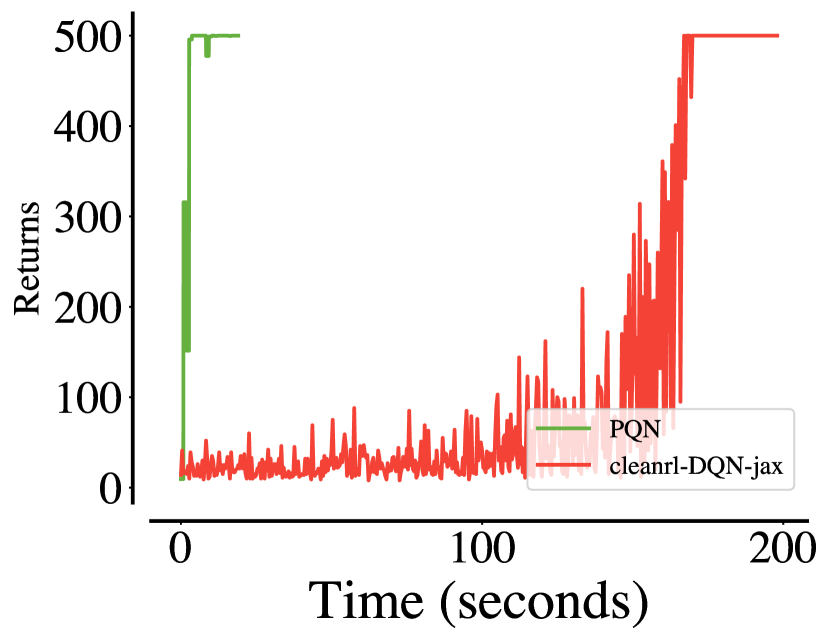
(a) CartPole:Training Time

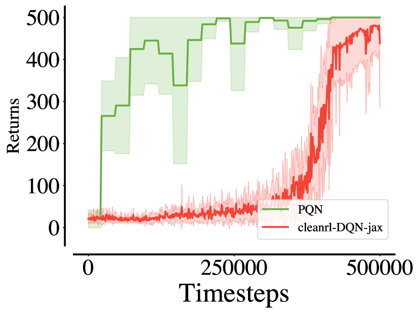
(b) CartPole: 10 Seeds

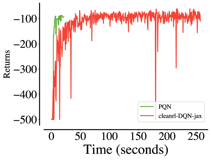
(c) Acrobot: Training Time

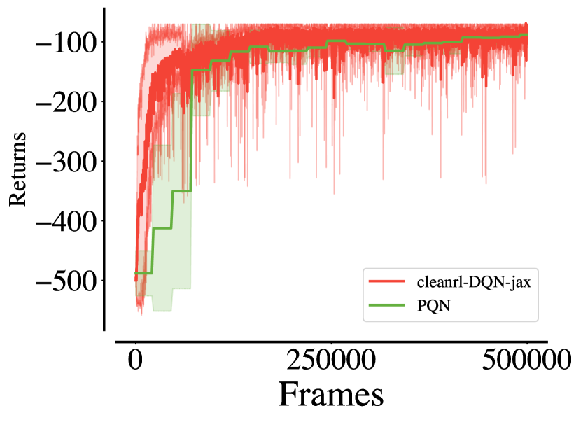
(d) Acrobot: 10 Seeds

Figure 8: Results in classic control tasks. The goal of this comparison is to show the time boost of PQN relative to a traditional DQN agent running a single environment in the cpu. PQN is compiled to run entirely on gpu, achieving a 10x speed-up compared to the standard DQN pipeline.

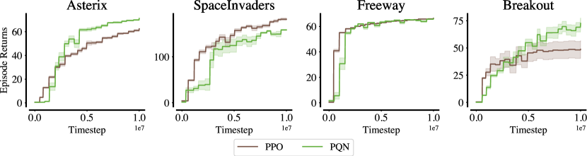
Figure 9: Results in MinAtar

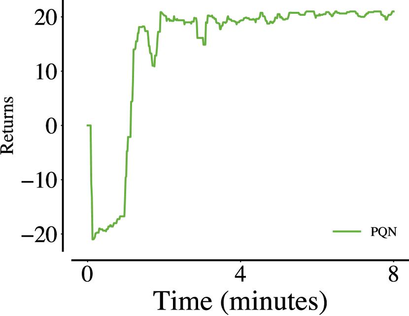
(a) Atari-Pong: PQN training

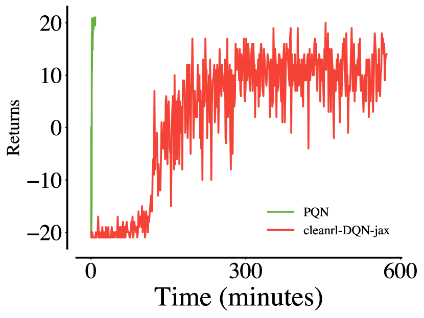
(b) Atari-Pong: Time Comparison

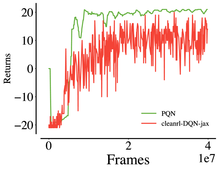
(c) Atari-Pong: Performances

Figure 10: Comparison between training a Q-Learning agent in Atari-Pong with PQN and the CleanRL implementation of DQN. PQN can solve the game by reaching a score of 20 in less than 4 minutes, while DQN requires almost 6 hours. As shown in the plot on the right, this doesn’t result in a loss of sample efficiency, as traditional distributed systems like Ape-X need more than 100 million frames to solve this simple game.

Table 3: Scores in ALE.

Method (Frames)	Time	Gradient	Atari-10	Atari-57	Atari-57	Atari-57
	(hours)	Steps	Score	Median	Mean	>Human
PPO (200M)	2.5	700k	165
PQN (200M)	1	700k	191
PQN (400M)	2	1.4M	243	245	1440	40
Rainbow (200M)	100	50M	239	230	1461	43

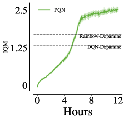
Figure 11: IQM computed over 3 seeds when training PQN with the ALE configuration proposed by Dopamine [13]. This configuration incorporates sticky actions and doesn’t set the done flag when an agent loses a life. With this setup, PQN can still outperform Rainbow, but it requires significantly more compute time (almost 5 hours), corresponding to 800 million frames, indicating a loss of sample efficiency. Sample efficiency might be recovered in this configuration by using a larger network or tuning the hyperparameters, but we leave this as future work. PQN is still much faster to train than a Dopamine agent, which requires multiple days depending on the hardware.

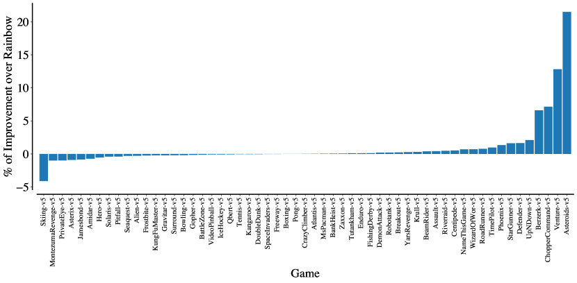
Figure 12: Improvement of PQN over Rainbow. Results refer to PQN trained for 400M frames, i.e. 2 hours of GPU time.

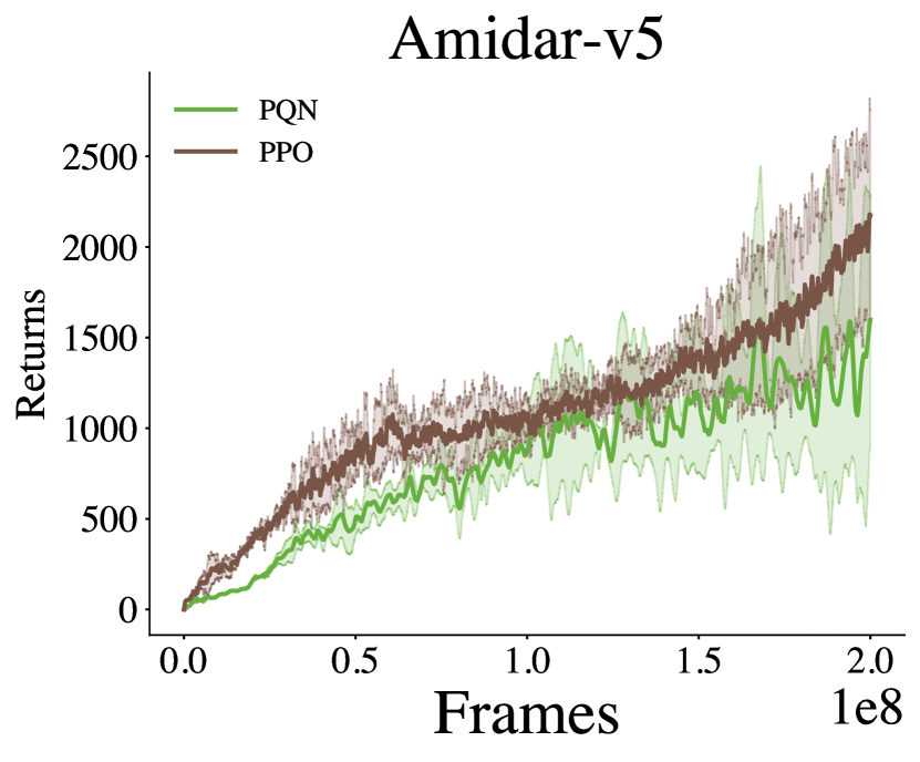
(a) Amidar

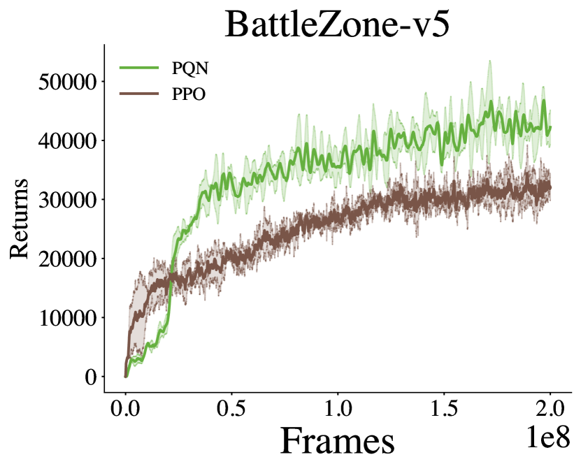
(b) BattleZone

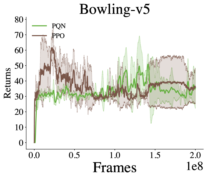
(c) Bowling

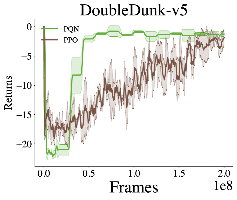
(d) DoubleDunk

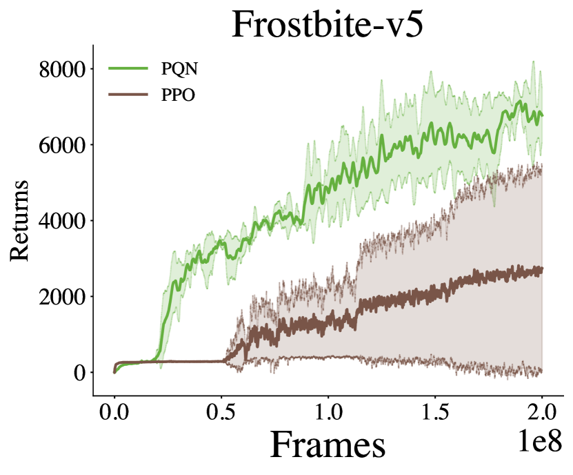
(e) Frostbite

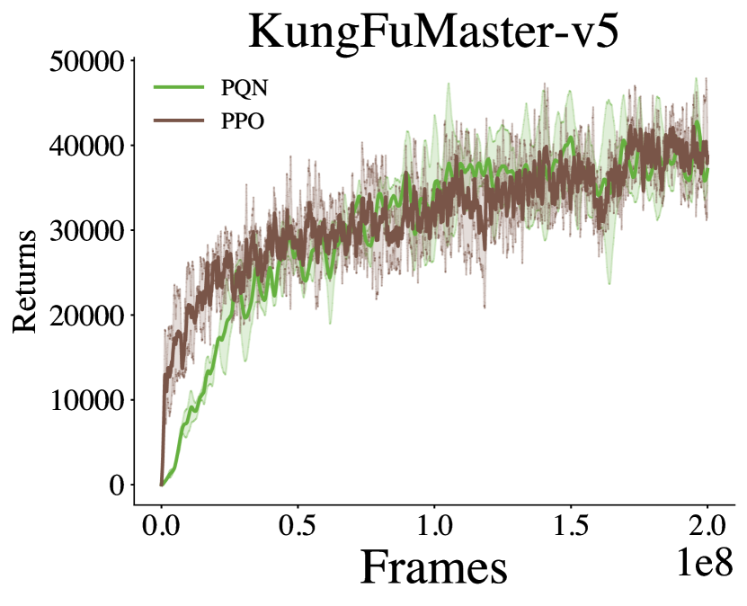
(f) KungFuMaster

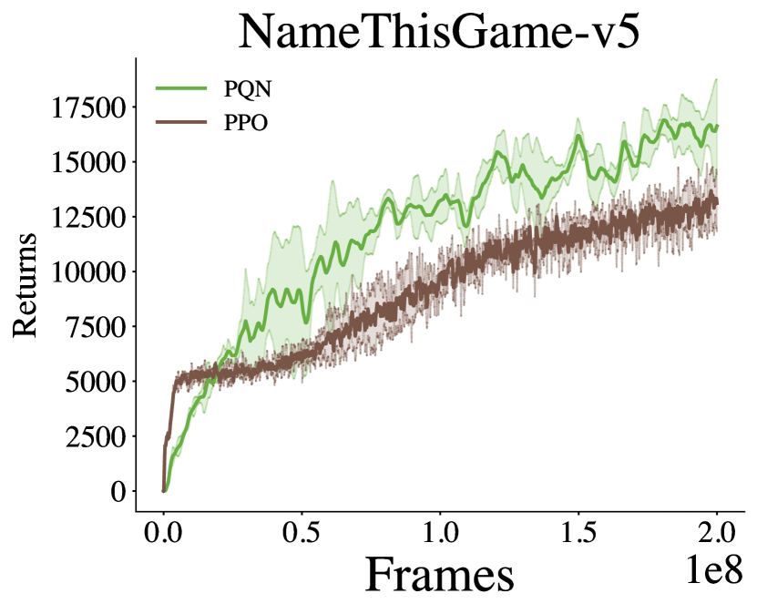
(g) NameThisGame

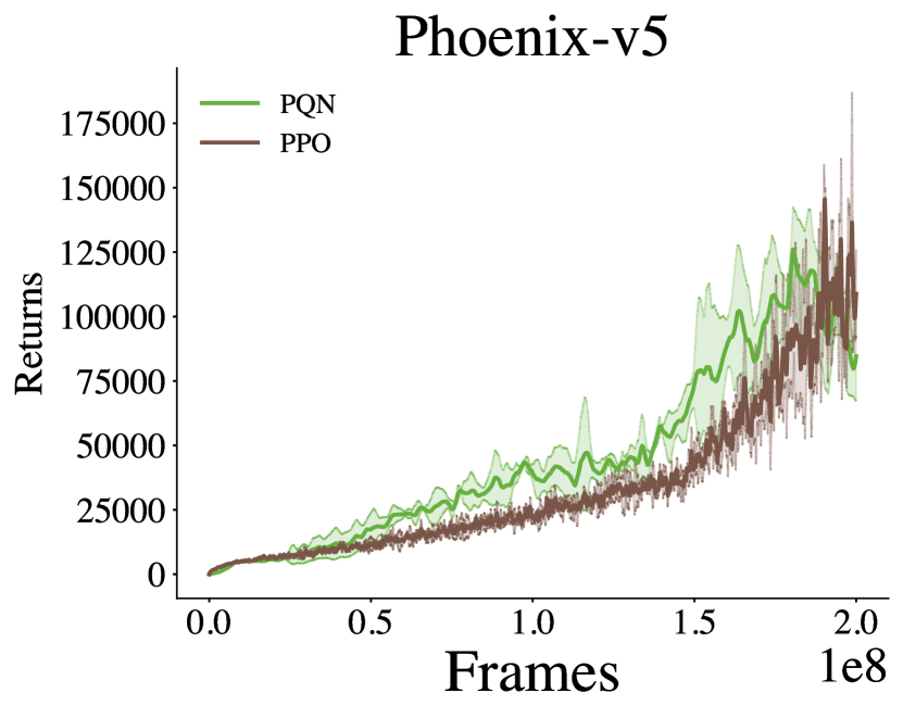
(h) Phoenix

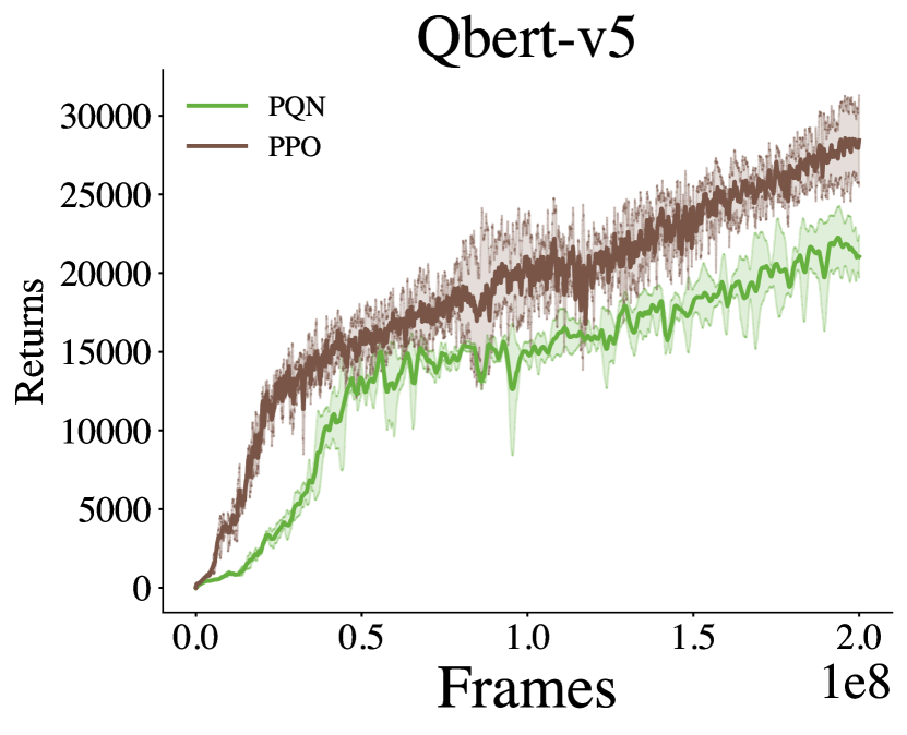
(i) Qbert

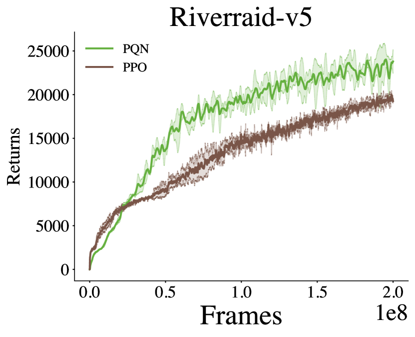
(j) Riverraid

Figure 13: Atari 10 Games Results

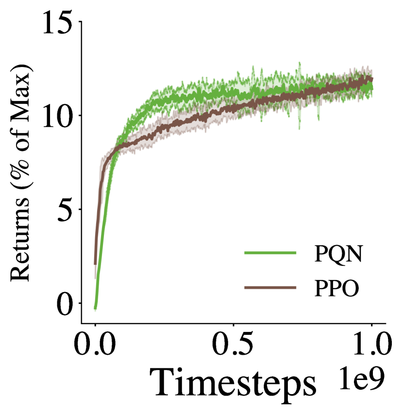
(a) Craftax with MLP networks

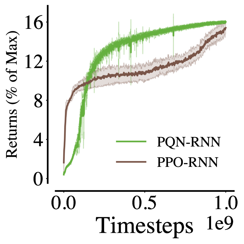
(b) Craftax with RNN networks

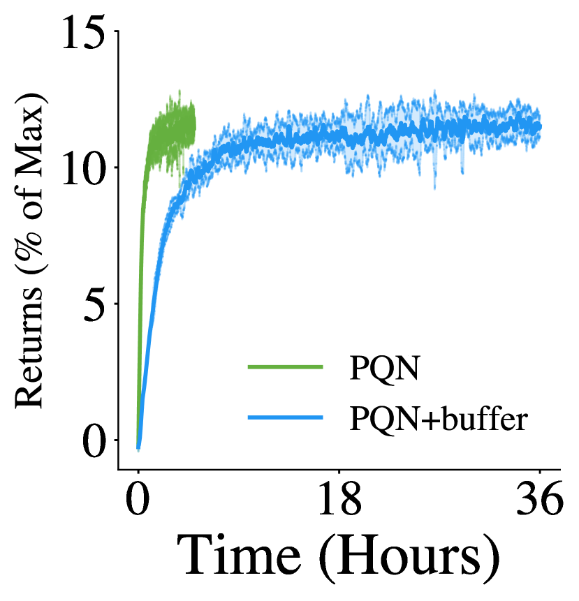
(c) Craftax with MLP and Buffer

Figure 14: Left: comparison between PPO and PQN in Craftax. Center: comparison with RNN versions of the two algorithms. Right: time to learn for 1e9 timesteps keeping a replay buffer in GPU.

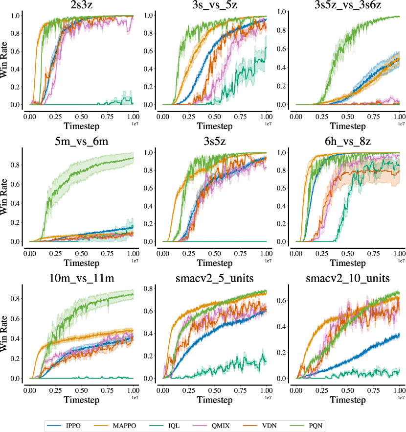
Figure 15: Results in Smax

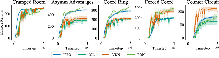
Figure 17: Results in Overcooked

H Method Time (hours) Mean Max MAPPO 15 23.9$\pm$0.02 24.23 PQN-VDN 10 24.37$\pm$0.04 24.45 PQN (2B) 2 24.1$\pm$0.1 24.22 R2D2-VDN 40 24.27$\pm$0.01 24.33

Table 4: Scores in 2-player Hanabi.

Appendix H Hyperparameters

Table 5: Craftax Hyperparameters

Parameter	Value
NUM_STEPS	1
NUM_ENVS	1024
HIDDEN_SIZE	512
N_LAYERS	2
EPS_START	0.1
EPS_FINISH	0.005
EPS_DECAY	0.2
NUM_EPOCHS	1
NUM_MINIBATCHES	1
LR	0.0001
MAX_GRAD_NORM	1.0
LR_LINEAR_DECAY	True
GAMMA	0.99

Table 6: Craftax RNN Hyperparameters

Parameter	Value
NUM_ENVs	1024
NUM_STEPS	128
EPS_START	1.0
EPS_FINISH	0.005
EPS_DECAY	0.1
NUM_MINIBATCHES	4
NUM_EPOCHS	4
NORM_INPUT	True
NORM_TYPE	"batch_norm"
HIDDEN_SIZE	512
NUM_LAYERS	1
NUM_RNN_LAYERS	1
ADD_LAST_ACTION	True
LR	0.0003
MAX_GRAD_NORM	0.5
LR_LINEAR_DECAY	True
REW_SCALE	1.0
GAMMA	0.99
LAMBDA	0.5

Table 7: Atari Hyperparameters

Parameter	Value
NUM_ENVs	128
NUM_STEPS	32
EPS_START	1.0
EPS_FINISH	0.001
EPS_DECAY	0.1
NUM_EPOCHS	2
NUM_MINIBATCHES	32
NORM_INPUT	False
NORM_TYPE	"layer_norm"
LR	0.00025
MAX_GRAD_NORM	10
LR_LINEAR_DECAY	False
GAMMA	0.99
LAMBDA	0.65

Table 8: SMAX Hyperparameters

Parameter	Value
NUM_ENVs	128
MEMORY_WINDOW	4
NUM_STEPS	128
HIDDEN_SIZE	512
NUM_LAYERS	2
NORM_INPUT	True
NORM_TYPE	"batch_norm"
EPS_START	1.0
EPS_FINISH	0.01
EPS_DECAY	0.1
MAX_GRAD_NORM	1
NUM_MINIBATCHES	16
NUM_EPOCHS	4
LR	0.00025
LR_LINEAR_DECAY	True
GAMMA	0.99
LAMBDA	0.85

Table 9: Overcooked Hyperparameters

Parameter	Value
NUM_ENVs	64
NUM_STEPS	16
HIDDEN_SIZE	512
NUM_LAYERS	2
NORM_INPUT	False
NORM_TYPE	"layer_norm"
EPS_START	1.0
EPS_FINISH	0.2
EPS_DECAY	0.2
MAX_GRAD_NORM	10
NUM_MINIBATCHES	16
NUM_EPOCHS	4
LR	0.000075
LR_LINEAR_DECAY	True
GAMMA	0.99
LAMBDA	0.5

Table 10: Hanabi Hyperparameters

Parameter	Value
NUM_ENVS	1024
NUM_STEPS	1
TOTAL_TIMESTEPS	1e10
HIDDEN_SIZE	512
N_LAYERS	3
NORM_TYPE	layer_norm
DUELING	True
EPS_START	0.01
EPS_FINISH	0.001
EPS_DECAY	0.1
MAX_GRAD_NORM	0.5
NUM_MINIBATCHES	1
NUM_EPOCHS	1
LR	0.0003
LR_LINEAR_DECAY	False
GAMMA	0.99

Game Rainbow PQN Alien 9491.70 6970.42 Amidar 5131.20 1408.15 Assault 14198.50 20089.42 Asterix 428200.30 38708.98 Asteroids 2712.80 45573.75 Atlantis 826659.50 845520.83 BankHeist 1358.00 1431.25 BattleZone 62010.00 54791.67 BeamRider 16850.20 23338.83 Berzerk 2545.60 18542.20 Bowling 30.00 28.71 Boxing 99.60 99.63 Breakout 417.50 515.08 Centipede 8167.30 11347.98 ChopperCommand 16654.00 129962.50 CrazyClimber 168788.50 171579.17 Defender 55105.00 140741.67 DemonAttack 111185.20 133075.21 DoubleDunk -0.30 -0.92 Enduro 2125.90 2349.17 FishingDerby 31.30 46.17 Freeway 34.00 33.75 Frostbite 9590.50 7313.54 Gopher 70354.60 60259.17 Gravitar 1419.30 1158.33 Hero 55887.40 26099.17 IceHockey 1.10 0.17 Jamesbond 20000.00 3254.17 Kangaroo 14637.50 14116.67 Krull 8741.50 10853.33 KungFuMaster 52181.00 41033.33 MontezumaRevenge 384.00 0.00 MsPacman 5380.40 5567.50 NameThisGame 13136.00 20603.33 Phoenix 108528.60 252173.33 Pitfall 0.00 -89.21 Pong 20.90 20.92 PrivateEye 4234.00 100.00 Qbert 33817.50 31716.67 Riverraid 20000.00 28764.27 RoadRunner 62041.00 109742.71 Robotank 61.40 73.96 Seaquest 15898.90 11345.00 Skiing -12957.80 -29975.31 Solaris 3560.30 2607.50 SpaceInvaders 18789.00 18450.83 StarGunner 127029.00 331300.00 Surround 9.70 5.88 Tennis 0.00 -1.04 TimePilot 12926.00 21950.00 Tutankham 241.00 264.71 UpNDown 100000.00 308327.92 Venture 5.50 76.04 VideoPinball 533936.50 489716.33 WizardOfWor 17862.50 30192.71 YarsRevenge 102557.00 129463.79 Zaxxon 22209.50 23537.50

Table 11: ALE Scores: Rainbow vs PQN (400M frames)

References

- Aitchison et al. [2023] Matthew Aitchison, Penny Sweetser, and Marcus Hutter. Atari-5: Distilling the arcade learning environment down to five games. In International Conference on Machine Learning, pages 421–438. PMLR, 2023.
- Ba et al. [2016] Jimmy Lei Ba, Jamie Ryan Kiros, and Geoffrey E. Hinton. Layer normalization. arXiv preprint arXiv:1607.06450, 2016.
- Badia et al. [2020] Adrià Puigdomènech Badia, Bilal Piot, Steven Kapturowski, Pablo Sprechmann, Alex Vitvitskyi, Zhaohan Daniel Guo, and Charles Blundell. Agent57: Outperforming the atari human benchmark. In International Conference on Machine Learning (ICML), pages 507–517. PMLR, 2020.
- Baird [1995] Leemon Baird. Residual algorithms: Reinforcement learning with function approximation. In Proceedings of the Twelfth International Conference on Machine Learning (ICML), pages 30–37, 1995. doi: 10.1.1.48.3256.
- Bard et al. [2020] Nolan Bard, Jakob N Foerster, Sarath Chandar, Neil Burch, Marc Lanctot, H Francis Song, Emilio Parisotto, Vincent Dumoulin, Subhodeep Moitra, Edward Hughes, et al. The Hanabi challenge: A new frontier for ai research. Artificial Intelligence, 280:103216, 2020.
- Bellemare et al. [2013] Marc G Bellemare, Yavar Naddaf, Joel Veness, and Michael Bowling. The arcade learning environment: An evaluation platform for general agents. Journal of Artificial Intelligence Research, 47:253–279, 2013.
- Bellman [1957] Richard Bellman. A markovian decision process. Journal of Mathematics and Mechanics, 6(5):679–684, 1957. ISSN 00959057, 19435274. URL http://www.jstor.org/stable/24900506.
- Bhandari et al. [2018] Jalaj Bhandari, Daniel Russo, and Raghav Singal. A finite time analysis of temporal difference learning with linear function approximation. arXiv preprint arXiv:1806.02450, 2018.
- Bhatt et al. [2024] Aditya Bhatt, Daniel Palenicek, Boris Belousov, Max Argus, Artemij Amiranashvili, Thomas Brox, and Jan Peters. Crossq: Batch normalization in deep reinforcement learning for greater sample efficiency and simplicity. In The Twelfth International Conference on Learning Representations, 2024. URL https://openreview.net/forum?id=PczQtTsTIX.
- Bonnet et al. [2024] Clément Bonnet, Daniel Luo, Donal Byrne, Shikha Surana, Sasha Abramowitz, Paul Duckworth, Vincent Coyette, Laurence I. Midgley, Elshadai Tegegn, Tristan Kalloniatis, Omayma Mahjoub, Matthew Macfarlane, Andries P. Smit, Nathan Grinsztajn, Raphael Boige, Cemlyn N. Waters, Mohamed A. Mimouni, Ulrich A. Mbou Sob, Ruan de Kock, Siddarth Singh, Daniel Furelos-Blanco, Victor Le, Arnu Pretorius, and Alexandre Laterre. Jumanji: a diverse suite of scalable reinforcement learning environments in jax, 2024. URL https://arxiv.org/abs/2306.09884.
- Borkar [2008] Vivek Borkar. Stochastic Approximation: A Dynamical Systems Viewpoint. Hindustan Book Agency Gurgaon, 01 2008. ISBN 978-81-85931-85-2. doi: 10.1007/978-93-86279-38-5.
- Carroll et al. [2019] Micah Carroll, Rohin Shah, Mark K Ho, Tom Griffiths, Sanjit Seshia, Pieter Abbeel, and Anca Dragan. On the utility of learning about humans for human-ai coordination. Advances in neural information processing systems, 32, 2019.
- Castro et al. [2018] Pablo Samuel Castro, Subhodeep Moitra, Carles Gelada, Saurabh Kumar, and Marc G. Bellemare. Dopamine: A Research Framework for Deep Reinforcement Learning. 2018. URL http://arxiv.org/abs/1812.06110.
- Chen et al. [2021] Xinyue Chen, Che Wang, Zijian Zhou, and Keith W. Ross. Randomized ensembled double q-learning: Learning fast without a model. The Ninth International Conference on Learning Representations (ICLR), abs/2101.05982, 2021.
- Dalal et al. [2017] Gal Dalal, Balázs Szörényi, Gugan Thoppe, and Shie Mannor. Finite sample analysis for TD(0) with linear function approximation. arXiv preprint arXiv:1704.01161, 2017.
- Daley and Amato [2019] Brett Daley and Christopher Amato. Reconciling -returns with experience replay. Advances in Neural Information Processing Systems, 32, 2019.
- Dayan [1992] Peter Dayan. The convergence of TD() for general . Mach. Learn., 8(3–4):341–362, May 1992. ISSN 0885-6125. doi: 10.1007/BF00992701. URL https://doi.org/10.1007/BF00992701.
- De Witt et al. [2020] Christian Schroeder De Witt, Tarun Gupta, Denys Makoviichuk, Viktor Makoviychuk, Philip HS Torr, Mingfei Sun, and Shimon Whiteson. Is independent learning all you need in the starcraft multi-agent challenge? arXiv preprint arXiv:2011.09533, 2020.
- Ellis et al. [2024] Benjamin Ellis, Jonathan Cook, Skander Moalla, Mikayel Samvelyan, Mingfei Sun, Anuj Mahajan, Jakob Foerster, and Shimon Whiteson. SMACv2: An improved benchmark for cooperative multi-agent reinforcement learning. Advances in Neural Information Processing Systems, 36, 2024.
- Engstrom et al. [2020] Logan Engstrom, Andrew Ilyas, Shibani Santurkar, Dimitris Tsipras, Firdaus Janoos, Larry Rudolph, and Aleksander Madry. Implementation matters in deep policy gradients: A case study on ppo and trpo. In International Conference on Learning Representations, 2020.
- Fellows et al. [2023] Mattie Fellows, Matthew Smith, and Shimon Whiteson. Why target networks stabilise temporal difference methods. In International Conference on Machine Learning, 2023.
- Foerster et al. [2018] Jakob Foerster, Gregory Farquhar, Triantafyllos Afouras, Nantas Nardelli, and Shimon Whiteson. Counterfactual multi-agent policy gradients. In Proceedings of the Thirty-Second AAAI Conference on Artificial Intelligence, page 2974–2982, 2018.
- Fujimoto et al. [2018] Scott Fujimoto, Herke van Hoof, and David Meger. Addressing function approximation error in actor-critic methods. International Conference on Machine Learning, abs/1802.09477, 2018.
- Gilks et al. [1995] W.R. Gilks, S. Richardson, and D. Spiegelhalter. Markov Chain Monte Carlo in Practice, chapter Introduction to General State-Space Markov Chain Theory. Chapman & Hall/CRC Interdisciplinary Statistics. Taylor & Francis, 1995. ISBN 9780412055515.
- Gu et al. [2023] Jiayuan Gu, Fanbo Xiang, Xuanlin Li, Zhan Ling, Xiqiang Liu, Tongzhou Mu, Yihe Tang, Stone Tao, Xinyue Wei, Yunchao Yao, Xiaodi Yuan, Pengwei Xie, Zhiao Huang, Rui Chen, and Hao Su. Maniskill2: A unified benchmark for generalizable manipulation skills. In International Conference on Learning Representations, 2023.
- Haarnoja et al. [2017] Tuomas Haarnoja, Haoran Tang, Pieter Abbeel, and Sergey Levine. Reinforcement learning with deep energy-based policies. In Doina Precup and Yee Whye Teh, editors, Proceedings of the 34th International Conference on Machine Learning, volume 70 of Proceedings of Machine Learning Research, pages 1352–1361, International Convention Centre, Sydney, Australia, 06–11 Aug 2017. PMLR. URL http://proceedings.mlr.press/v70/haarnoja17a.html.
- Haarnoja et al. [2018] Tuomas Haarnoja, Aurick Zhou, Pieter Abbeel, and Sergey Levine. Soft Actor-Critic: Off-policy maximum entropy deep reinforcement learning with a stochastic actor. In Jennifer Dy and Andreas Krause, editors, Proceedings of the 35th International Conference on Machine Learning, volume 80 of Proceedings of Machine Learning Research, pages 1861–1870, Stockholmsmässan, Stockholm Sweden, 10–15 Jul 2018. PMLR. URL http://proceedings.mlr.press/v80/haarnoja18b.html.
- Hafner [2021] Danijar Hafner. Benchmarking the spectrum of agent capabilities. In The Ninth International Conference on Learning Representations, 2021.
- Hessel et al. [2018] Matteo Hessel, Joseph Modayil, Hado Van Hasselt, Tom Schaul, Georg Ostrovski, Will Dabney, Dan Horgan, Bilal Piot, Mohammad Azar, and David Silver. Rainbow: Combining improvements in deep reinforcement learning. In Proceedings of the Thirty-Second Conference on Uncertainty in Artificial Intelligence, 2018.
- Hoffman et al. [2020] Matthew W. Hoffman, Bobak Shahriari, John Aslanides, Gabriel Barth-Maron, Nikola Momchev, Danila Sinopalnikov, Piotr Stańczyk, Sabela Ramos, Anton Raichuk, Damien Vincent, Léonard Hussenot, Robert Dadashi, Gabriel Dulac-Arnold, Manu Orsini, Alexis Jacq, Johan Ferret, Nino Vieillard, Seyed Kamyar Seyed Ghasemipour, Sertan Girgin, Olivier Pietquin, Feryal Behbahani, Tamara Norman, Abbas Abdolmaleki, Albin Cassirer, Fan Yang, Kate Baumli, Sarah Henderson, Abe Friesen, Ruba Haroun, Alex Novikov, Sergio Gómez Colmenarejo, Serkan Cabi, Caglar Gulcehre, Tom Le Paine, Srivatsan Srinivasan, Andrew Cowie, Ziyu Wang, Bilal Piot, and Nando de Freitas. Acme: A research framework for distributed reinforcement learning. arXiv preprint arXiv:2006.00979, 2020. URL https://arxiv.org/abs/2006.00979.
- Horgan et al. [2018] Dan Horgan, John Quan, David Budden, Gabriel Barth-Maron, Matteo Hessel, Hado Van Hasselt, and David Silver. Distributed prioritized experience replay. arXiv preprint arXiv:1803.00933, 2018.
- Hu et al. [2021] Hengyuan Hu, Adam Lerer, Brandon Cui, Luis Pineda, Noam Brown, and Jakob Foerster. Off-belief learning. In International Conference on Machine Learning, pages 4369–4379. PMLR, 2021.
- Huang et al. [2022a] Shengyi Huang, Rousslan Fernand Julien Dossa, Antonin Raffin, Anssi Kanervisto, and Weixun Wang. The 37 implementation details of proximal policy optimization. In ICLR Blog Track, 2022a. URL https://iclr-blog-track.github.io/2022/03/25/ppo-implementation-details/. https://iclr-blog-track.github.io/2022/03/25/ppo-implementation-details/.
- Huang et al. [2022b] Shengyi Huang, Rousslan Fernand Julien Dossa, Chang Ye, Jeff Braga, Dipam Chakraborty, Kinal Mehta, and João G.M. Araújo. Cleanrl: High-quality single-file implementations of deep reinforcement learning algorithms. Journal of Machine Learning Research, 23(274):1–18, 2022b. URL http://jmlr.org/papers/v23/21-1342.html.
- Ioffe and Szegedy [2015] Sergey Ioffe and Christian Szegedy. Batch normalization: accelerating deep network training by reducing internal covariate shift. In Proceedings of the 32nd International Conference on International Conference on Machine Learning - Volume 37, ICML’15, page 448–456. JMLR.org, 2015.
- Kapturowski et al. [2018] Steven Kapturowski, Georg Ostrovski, John Quan, Remi Munos, and Will Dabney. Recurrent experience replay in distributed reinforcement learning. In The Sixth International Conference on Learning Representations (ICLR), 2018.
- Keskar et al. [2016] Nitish Shirish Keskar, Dheevatsa Mudigere, Jorge Nocedal, Mikhail Smelyanskiy, and Ping Tak Peter Tang. On large-batch training for deep learning: Generalization gap and sharp minima. arXiv preprint arXiv:1609.04836, 2016.
- Kozuno et al. [2021] Tadashi Kozuno, Yunhao Tang, Mark Rowland, Remi Munos, Steven Kapturowski, Will Dabney, Michal Valko, and David Abel. Revisiting peng’s q(lambda) for modern reinforcement learning. In Marina Meila and Tong Zhang, editors, Proceedings of the 38th International Conference on Machine Learning, volume 139 of Proceedings of Machine Learning Research, pages 5794–5804. PMLR, 18–24 Jul 2021. URL https://proceedings.mlr.press/v139/kozuno21a.html.
- Küttler et al. [2020] Heinrich Küttler, Nantas Nardelli, Alexander Miller, Roberta Raileanu, Marco Selvatici, Edward Grefenstette, and Tim Rocktäschel. The nethack learning environment. Advances in Neural Information Processing Systems, 33:7671–7684, 2020.
- Laidlaw et al. [2024] Cassidy Laidlaw, Banghua Zhu, Stuart J. Russell, and Anca Dragan. The effective horizon explains deep RL performance in stochastic environments. arXiv preprint arXiv:2312.08369, 2024. URL https://arxiv.org/pdf/2312.08369.
- Lange [2022] Robert Tjarko Lange. gymnax: A JAX-based reinforcement learning environment library, 2022. URL http://github.com/RobertTLange/gymnax.
- Lee et al. [2019] Jaehoon Lee, Lechao Xiao, Samuel S. Schoenholz, Yasaman Bahri, Roman Novak, Jascha Sohl-Dickstein, and Jeffrey Pennington. Wide neural networks of any depth evolve as linear models under gradient descent. In Proceedings of the 33rd International Conference on Neural Information Processing Systems, Red Hook, NY, USA, 2019. Curran Associates Inc.
- Li et al. [2023] Zechu Li, Tao Chen, Zhang-Wei Hong, Anurag Ajay, and Pulkit Agrawal. Parallel -learning: Scaling off-policy reinforcement learning under massively parallel simulation. In International Conference on Machine Learning, pages 19440–19459. PMLR, 2023.
- Liu et al. [2019] Liyuan Liu, Haoming Jiang, Pengcheng He, Weizhu Chen, Xiaodong Liu, Jianfeng Gao, and Jiawei Han. On the variance of the adaptive learning rate and beyond. arXiv preprint arXiv:1908.03265, 2019.
- Lowe et al. [2017] Ryan Lowe, Aviv Tamar, Jean Harb, OpenAI Pieter Abbeel, and Igor Mordatch. Multi-agent actor-critic for mixed cooperative-competitive environments. Advances in neural information processing systems, 30, 2017.
- Lu et al. [2022] Chris Lu, Jakub Kuba, Alistair Letcher, Luke Metz, Christian Schroeder de Witt, and Jakob Foerster. Discovered policy optimisation. Advances in Neural Information Processing Systems, 35:16455–16468, 2022.
- Lyle et al. [2023] Clare Lyle, Zeyu Zheng, Evgenii Nikishin, Bernardo Avila Pires, Razvan Pascanu, and Will Dabney. Understanding plasticity in neural networks. In International Conference on Machine Learning, pages 23190–23211. PMLR, 2023.
- Lyle et al. [2024] Clare Lyle, Zeyu Zheng, Khimya Khetarpal, Hado van Hasselt, Razvan Pascanu, James Martens, and Will Dabney. Disentangling the causes of plasticity loss in neural networks. arXiv preprint arXiv:2402.18762, 2024.
- Makoviychuk et al. [2021] Viktor Makoviychuk, Lukasz Wawrzyniak, Yunrong Guo, Michelle Lu, Kier Storey, Miles Macklin, David Hoeller, Nikita Rudin, Arthur Allshire, Ankur Handa, and Gavriel State. Isaac gym: High performance gpu-based physics simulation for robot learning, 2021.
- Matthews et al. [2024a] Michael Matthews, Michael Beukman, Benjamin Ellis, Mikayel Samvelyan, Matthew Jackson, Samuel Coward, and Jakob Foerster. Craftax: A lightning-fast benchmark for open-ended reinforcement learning. arXiv preprint arXiv:2402.16801, 2024a.
- Matthews et al. [2024b] Michael Matthews, Michael Beukman, Benjamin Ellis, Mikayel Samvelyan, Matthew Jackson, Samuel Coward, and Jakob Foerster. Craftax: A lightning-fast benchmark for open-ended reinforcement learning. arXiv preprint arXiv:2402.16801, 2024b.
- Mnih et al. [2013] Volodymyr Mnih, Koray Kavukcuoglu, David Silver, Alex Graves, Ioannis Antonoglou, Daan Wierstra, and Martin Riedmiller. Playing atari with deep reinforcement learning. arXiv preprint arXiv:1312.5602, 2013. URL http://arxiv.org/abs/1312.5602. cite arxiv:1312.5602Comment: NIPS Deep Learning Workshop 2013.
- Mnih et al. [2015] Volodymyr Mnih, Koray Kavukcuoglu, David Silver, Andrei A. Rusu, Joel Veness, Marc G. Bellemare, Alex Graves, Martin Riedmiller, Andreas K. Fidjeland, Georg Ostrovski, Stig Petersen, Charles Beattie, Amir Sadik, Ioannis Antonoglou, Helen King, Dharshan Kumaran, Daan Wierstra, Shane Legg, and Demis Hassabis. Human-level control through deep reinforcement learning. Nature, 518(7540):529–533, February 2015. ISSN 00280836. URL http://dx.doi.org/10.1038/nature14236.
- Mnih et al. [2016] Volodymyr Mnih, Adria Puigdomenech Badia, Mehdi Mirza, Alex Graves, Timothy Lillicrap, Tim Harley, David Silver, and Koray Kavukcuoglu. Asynchronous methods for deep reinforcement learning. In Maria Florina Balcan and Kilian Q. Weinberger, editors, Proceedings of The 33rd International Conference on Machine Learning, volume 48 of Proceedings of Machine Learning Research, pages 1928–1937, New York, New York, USA, 20–22 Jun 2016. PMLR. URL https://proceedings.mlr.press/v48/mniha16.html.
- Obando Ceron et al. [2024] Johan Obando Ceron, Marc Bellemare, and Pablo Samuel Castro. Small batch deep reinforcement learning. Advances in Neural Information Processing Systems, 36, 2024.
- Osband et al. [2016] Ian Osband, Charles Blundell, Alexander Pritzel, and Benjamin Van Roy. Deep exploration via bootstrapped dqn. In D. Lee, M. Sugiyama, U. Luxburg, I. Guyon, and R. Garnett, editors, Advances in Neural Information Processing Systems, volume 29. Curran Associates, Inc., 2016. URL https://proceedings.neurips.cc/paper_files/paper/2016/file/8d8818c8e140c64c743113f563cf750f-Paper.pdf.
- Osband et al. [2019] Ian Osband, Yotam Doron, Matteo Hessel, John Aslanides, Eren Sezener, Andre Saraiva, Katrina McKinney, Tor Lattimore, Csaba Szepesvari, Satinder Singh, et al. Behaviour suite for reinforcement learning. arXiv preprint arXiv:1908.03568, 2019.
- Peng and Williams [1994] Jing Peng and Ronald J. Williams. Incremental multi-step q-learning. In William W. Cohen and Haym Hirsh, editors, Machine Learning Proceedings 1994, pages 226–232. Morgan Kaufmann, San Francisco (CA), 1994. ISBN 978-1-55860-335-6. doi: https://doi.org/10.1016/B978-1-55860-335-6.50035-0. URL https://www.sciencedirect.com/science/article/pii/B9781558603356500350.
- Puterman [2014] Martin L Puterman. Markov decision processes: discrete stochastic dynamic programming. John Wiley & Sons, 2014.
- Rashid et al. [2020a] Tabish Rashid, Mikayel Samvelyan, Christian Schroeder De Witt, Gregory Farquhar, Jakob Foerster, and Shimon Whiteson. Monotonic value function factorisation for deep multi-agent reinforcement learning. Journal of Machine Learning Research, 21(178):1–51, 2020a.
- Rashid et al. [2020b] Tabish Rashid, Mikayel Samvelyan, Christian Schroeder De Witt, Gregory Farquhar, Jakob Foerster, and Shimon Whiteson. Monotonic value function factorisation for deep multi-agent reinforcement learning. Journal of Machine Learning Research, 21(178):1–51, 2020b.
- Robbins and Monro [1951] Herbert Robbins and Sutton Monro. A Stochastic Approximation Method. The Annals of Mathematical Statistics, 22(3):400 – 407, 1951. doi: 10.1214/aoms/1177729586. URL https://doi.org/10.1214/aoms/1177729586.
- Rutherford et al. [2023] Alexander Rutherford, Benjamin Ellis, Matteo Gallici, Jonathan Cook, Andrei Lupu, Gardar Ingvarsson, Timon Willi, Akbir Khan, Christian Schroeder de Witt, Alexandra Souly, et al. Jaxmarl: Multi-agent rl environments in jax. arXiv preprint arXiv:2311.10090, 2023.
- Samvelyan et al. [2019] Mikayel Samvelyan, Tabish Rashid, Christian Schroeder De Witt, Gregory Farquhar, Nantas Nardelli, Tim GJ Rudner, Chia-Man Hung, Philip HS Torr, Jakob Foerster, and Shimon Whiteson. The starcraft multi-agent challenge. arXiv preprint arXiv:1902.04043, 2019.
- Schulman et al. [2015] John Schulman, Sergey Levine, Pieter Abbeel, Michael Jordan, and Philipp Moritz. Trust region policy optimization. In Francis Bach and David Blei, editors, Proceedings of the 32nd International Conference on Machine Learning, volume 37 of Proceedings of Machine Learning Research, pages 1889–1897, Lille, France, 07–09 Jul 2015. PMLR. URL https://proceedings.mlr.press/v37/schulman15.html.
- Schulman et al. [2017] John Schulman, Filip Wolski, Prafulla Dhariwal, Alec Radford, and Oleg Klimov. Proximal policy optimization algorithms. CoRR, abs/1707.06347, 2017. URL http://arxiv.org/abs/1707.06347.
- Son et al. [2019] Kyunghwan Son, Daewoo Kim, Wan Ju Kang, David Earl Hostallero, and Yung Yi. Qtran: Learning to factorize with transformation for cooperative multi-agent reinforcement learning. In International Conference on Machine Learning (ICML), pages 5887–5896. PMLR, 2019.
- Srikant and Ying [2019] Rayadurgam Srikant and Lei Ying. Finite-time error bounds for linear stochastic approximation and td learning. In Conference on Learning Theory, pages 2803–2830. PMLR, 2019.
- Sunehag et al. [2017a] Peter Sunehag, Guy Lever, Audrunas Gruslys, Wojciech Marian Czarnecki, Vinicius Zambaldi, Max Jaderberg, Marc Lanctot, Nicolas Sonnerat, Joel Z Leibo, Karl Tuyls, et al. Value-decomposition networks for cooperative multi-agent learning. arXiv preprint arXiv:1706.05296, 2017a.
- Sunehag et al. [2017b] Peter Sunehag, Guy Lever, Audrunas Gruslys, Wojciech Marian Czarnecki, Vinicius Zambaldi, Max Jaderberg, Marc Lanctot, Nicolas Sonnerat, Joel Z Leibo, Karl Tuyls, et al. Value-decomposition networks for cooperative multi-agent learning. arXiv preprint arXiv:1706.05296, 2017b.
- Sutton [1988] Richard S. Sutton. Learning to predict by the methods of temporal differences. Machine Learning, 3(1):9–44, Aug 1988. ISSN 1573-0565. doi: 10.1007/BF00115009.
- Sutton and Barto [2018a] Richard S. Sutton and Andrew G. Barto. Reinforcement Learning: An Introduction. The MIT Press, second edition, 2018a. URL http://incompleteideas.net/book/the-book-2nd.html.
- Sutton and Barto [2018b] Richard S Sutton and Andrew G Barto. Reinforcement learning: An introduction. MIT press, 2018b.
- Toledo et al. [2023] Edan Toledo, Laurence Midgley, Donal Byrne, Callum Rhys Tilbury, Matthew Macfarlane, Cyprien Courtot, and Alexandre Laterre. Flashbax: Streamlining experience replay buffers for reinforcement learning with jax, 2023. URL https://github.com/instadeepai/flashbax/.
- Towers et al. [2023] Mark Towers, Jordan K. Terry, Ariel Kwiatkowski, John U. Balis, Gianluca de Cola, Tristan Deleu, Manuel Goulão, Andreas Kallinteris, Arjun KG, Markus Krimmel, Rodrigo Perez-Vicente, Andrea Pierré, Sander Schulhoff, Jun Jet Tai, Andrew Tan Jin Shen, and Omar G. Younis. Gymnasium, March 2023. URL https://zenodo.org/record/8127025.
- Tsitsiklis and Van Roy [1997] J. N. Tsitsiklis and B. Van Roy. An analysis of temporal-difference learning with function approximation. IEEE Transactions on Automatic Control, 42(5):674–690, May 1997. ISSN 2334-3303. doi: 10.1109/9.580874.
- van Hasselt et al. [2018] Hado van Hasselt, Yotam Doron, Florian Strub, Matteo Hessel, Nicolas Sonnerat, and Joseph Modayil. Deep Reinforcement Learning and the Deadly Triad. working paper or preprint, December 2018. URL https://hal.science/hal-01949304.
- Wang and Blei [2017] Yixin Wang and David Blei. Frequentist consistency of variational bayes. Journal of the American Statistical Association, 05 2017. doi: 10.1080/01621459.2018.1473776.
- Wang et al. [2016] Ziyu Wang, Tom Schaul, Matteo Hessel, Hado Hasselt, Marc Lanctot, and Nando Freitas. Dueling network architectures for deep reinforcement learning. In International Conference on Machine Learning (ICML), pages 1995–2003. PMLR, 2016.
- Watkins and Dayan [1992] Christopher J. C. H. Watkins and Peter Dayan. Technical note: q -learning. Mach. Learn., 8(3–4):279–292, May 1992. ISSN 0885-6125. doi: 10.1007/BF00992698. URL https://doi.org/10.1007/BF00992698.
- Watkins [1989] Christopher John Cornish Hellaby Watkins. Learning from Delayed Rewards. PhD thesis, King’s College, University of Cambridge, Cambridge, UK, May 1989. URL http://www.cs.rhul.ac.uk/~chrisw/new_thesis.pdf.
- Weng et al. [2022] Jiayi Weng, Min Lin, Shengyi Huang, Bo Liu, Denys Makoviichuk, Viktor Makoviychuk, Zichen Liu, Yufan Song, Ting Luo, Yukun Jiang, Zhongwen Xu, and Shuicheng Yan. EnvPool: A highly parallel reinforcement learning environment execution engine. In S. Koyejo, S. Mohamed, A. Agarwal, D. Belgrave, K. Cho, and A. Oh, editors, Advances in Neural Information Processing Systems, volume 35, pages 22409–22421. Curran Associates, Inc., 2022. URL https://proceedings.neurips.cc/paper_files/paper/2022/file/8caaf08e49ddbad6694fae067442ee21-Paper-Datasets_and_Benchmarks.pdf.
- Williams [1991] David Williams. Probability with Martingales. Cambridge mathematical textbooks. Cambridge University Press, 1991. ISBN 978-0-521-40605-5.
- Young and Tian [2019] Kenny Young and Tian Tian. Minatar: An atari-inspired testbed for thorough and reproducible reinforcement learning experiments. arXiv preprint arXiv:1903.03176, 2019.
- Yu et al. [2022a] Chao Yu, Akash Velu, Eugene Vinitsky, Jiaxuan Gao, Yu Wang, Alexandre Bayen, and Yi Wu. The surprising effectiveness of ppo in cooperative multi-agent games. Advances in Neural Information Processing Systems, 35:24611–24624, 2022a.
- Yu et al. [2022b] Chao Yu, Akash Velu, Eugene Vinitsky, Jiaxuan Gao, Yu Wang, Alexandre Bayen, and Yi Wu. The surprising effectiveness of ppo in cooperative multi-agent games. Advances in Neural Information Processing Systems, 35:24611–24624, 2022b.