Factorization for $J/\psi$ leptoproduction at small transverse momentum

Abstract

Nonrelativistic Quantum Chromodynamics (NRQCD) breaks down in the region of low transverse momentum, where the transverse momentum of the produced quarkonium state is sensitive to multiple scattering with the incoming hadron and to soft gluon radiation. In this kinematic regime, the transverse-momentum-dependent (TMD) factorization framework is required, promoting the long-distance matrix elements (LDMEs) of NRQCD to the so-called TMD shape functions (TMDShFs), which encode both the soft gluon radiation and the formation of the heavy-quark bound state. In this work, we apply an effective-field theory approach (combining NRQCD and SCET) to the photon-gluon fusion process in inclusive $J/\psi$ leptoproduction. We derive a factorization theorem for the cross section in terms of TMDShFs, compute these quantities at next-to-leading order, establish their evolution, and study their matching onto the corresponding LDMEs in the high-transverse-momentum region. Our results are particularly relevant to the Electron-Ion Collider, where $J/\psi$ leptoproduction can be used to probe gluon transverse-momentum-dependent parton distribution functions (gluon TMDPDFs).

1 Introduction

Quarkonium production in semi-inclusive deep inelastic scattering (SIDIS) is a particularly valuable process for probing transverse-momentum-dependent (TMD) gluon distributions. Indeed, since heavy quarks couple to the gluon distribution already at leading order in the strong coupling, measuring the transverse momentum of the produced quarkonium state can give access to the incoming gluon’s transverse momentum. Therefore, particularly in the context of the future Electron-Ion Collider (EIC) AbdulKhalek:2021gbh , quarkonium production in SIDIS has already been studied extensively Fleming:1997fq ; Kniehl:2001tk ; Godbole:2013bca ; Mukherjee:2016qxa ; Rajesh:2018qks ; Bacchetta:2018ivt ; DAlesio:2019qpk ; Boer:2020bbd ; DAlesio:2021yws ; ColpaniSerri:2021bla ; Kishore:2022ddb ; Bor:2022fga ; DAlesio:2023qyo ; Boer:2023zit ; Kang:2023doo ; Maxia:2024cjh ; Kato:2024vzt . In addition, quarkonium production in pp collisions at the Large Hadron Collider (LHC) has been studied in, e.g. denDunnen:2014kjo ; Lansberg:2017tlc ; Lansberg:2017dzg ; Scarpa:2020sdy ; Scarpa:2019fol ; Wei:2024ksb , in $e^{+}e^{-}$ annihilation at B factories Jia:2024cvv ; Lee:2020dza and at Belle II Garg:2024rkt , in Z-boson decays at LHC Wang:2023ssg ; Bodwin:2017pzj , and in Higgs decay at HL-LHC Martynenko:2023xyx ; Dong:2022bkd (see also Chapon:2020heu for the prospects at HL-LHC), as well as many others (see Lansberg:2019adr for a comprehensive review). Moreover, recent work regarding quarkonium in fragmentation functions can be found in Echevarria:2020qjk ; Celiberto:2023fzz ; Dai:2023rvd ; Copeland:2023qed ; Echevarria:2023dme ; Copeland:2023wbu ; vonKuk:2024uxe .

The main goal of this paper is to establish the factorization for $J/\psi$ leptoproduction in terms of TMD shape functions (TMDShFs) and gluon TMD parton distribution functions Mulders:2000sh ; Meissner:2007rx ; Echevarria:2015uaa (gluon TMDPDFs). TMDShFs describe the formation of the quarkonium bound state, while gluon TMDPDFs parameterize the structure of the incoming hadron in terms of gluons. Both TMDShFs and gluon TMDPDFs are transverse-momentum dependent and highly sensitive to the soft gluon radiation involved in the entire process. Our aim is to develop a complete and consistent theoretical framework for quarkonium leptoproduction at small transverse momentum, describing its factorization in terms of TMDShFs and TMDPDFs, attributing the different modes of gluon radiation to the proper objects. Afterwards, we study the scale evolution of the TMDShFs as well as their matching onto collinear functions at high transverse momentum.

Nonrelativistic Quantum Chromodynamics (NRQCD) Bodwin:1994jh is an effective field theory (EFT) for the description of heavy quarkonium, using the relative velocity v of the heavy quark in the rest frame of the bound state as the power counting parameter. Quarkonium production is studied within the framework of the NRQCD factorization conjecture Nayak:2005rt ; Nayak:2005rw ; Kang:2011zza ; Kang:2014tta , where the cross section can be separated into two parts: the short-distance coefficients (SDCs) and the long-distance matrix elements (LDMEs). The SDCs encode the heavy-quark pair production and are calculable in perturbative QCD. The LDMEs, on the other hand, parameterize the probability that the heavy-quark pair with a specific spin $S$, angular momentum $L$, and color configuration (octet $[8]$ or singlet $[1]$), denoted as $[n]=\,^{2S+1}L_{J}^{[1,8]}$, hadronizes into the bound state. Therefore, LDMEs are inherently nonperturbative and need to be extracted from experiments, see, e.g., Butenschoen:2011yh ; Shao:2014yta ; Bodwin:2015iua ; Feng:2018ukp ; Brambilla:2022ayc . Not all the possible heavy-quark configurations contribute to the final quarkonium state, since LDMEs scale with powers of the relative velocity Braaten:1996ix and calculations are performed up to a fixed order in the v-expansion. In the case of the production of a $J/\psi$ meson, the leading power (LP) in the v-expansion corresponds to the color-singlet $[n]=\!\,^{3}S_{1}^{[1]}$ and the next-to-leading power (NLP) to the color-octet states ${}^{1}S_{0}^{[8]}$, ${}^{3}S_{1}^{[8]}$, and ${}^{3}P_{J}^{[8]}$, see, e.g., Schuler:1997is . In our work, we perform the calculations in the so-called vNRQCD framework Rothstein:2018dzq (briefly reviewed in appendix A), which is a formulation of NRQCD in which there is a clear separation between potential, soft, and ultrasoft (usoft) modes through the label-momentum notation. This separation is crucial in our analysis, since soft and usoft gluon radiation plays a central role in the process we are interested in, and heavy quarks couple to both.

Indeed, NRQCD factorization in terms of LDMEs is only well-defined when the heavy-quark pair is produced in the hard scattering with a large transverse momentum that remains largely unaffected by initial and final state radiation (see Braaten:1994kd ; Braaten:1994vv ; Ma:1995vi ; Braaten:1996rp ; Petrelli:1997ge ; Bodwin:2015iua ). In contrast, when the heavy-quark pair is produced with low transverse momentum $p_{T}\ll Q_{H}$ (with $Q_{H}$ the hard scale of the process), radiative corrections due to abundant gluon emissions become crucial. These emissions manifest as collinear, soft, and usoft modes, organized in the momentum region with the help of the scaling parameter $\lambda\equiv p_{T}/Q_{H}$, and are extensively studied within the framework of soft-collinear effective theory (SCET) Bauer:2000ew ; Bauer:2001yt ; Bauer:2001ct ; Beneke:2002ph , in particular $\text{SCET}_{\text{II}}$ Bauer:2002aj which includes soft particles with momentum scaling as $k^{\mu}\sim Q_{H}\lambda$. More specifically, as illustrated in figure 1, soft radiation at low transverse momentum becomes entangled with the (u)soft radiation responsible for the binding mechanism of the quarkonium pair, since the heavy quarks interact with both gluon modes. Therefore, in the low-transverse momentum region, the LDMEs must be promoted to TMDShFs which incorporate this soft+usoft radiation. In consequence, we need to work in the vNRQCD+SCET framework where the calculations can be organized according to two power-counting parameters in addition to the QCD coupling constant: v and $\lambda$, which determine the scaling in vNRQCD and SCET, respectively.

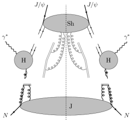
Figure 1: Diagrammatic representation of the factorization theorem for $\gamma^{*}\!+\!N\!\to\!J/\psi\!+\!X$ at small transverse momentum, which states that the cross section can be written as $d\sigma\!\sim\!|\text{H}|^{2}\!\otimes\!\text{J}\!\otimes\text{Sh}$. H describes the hard collision $\gamma^{*}\!+\!g\!\to\!c\bar{c}$, with the heavy-quark pair being created in a particular state $[n]\!=\!\,^{2S\!+\!1}L_{J}^{[1,8]}$. J stands for the gluon TMDPDF, where we have used a full line with arrow with a coil overlay to indicate the incoming collinear gluon. Finally, Sh stands for the TMDShF. The black and gray double lines indicate the collinear and soft Wilson lines, respectively (usoft Wilson lines are not drawn). The gray lines connecting Sh with the soft Wilson lines indicate the contribution of soft radiation in the two directions involved in the process.

The remainder of this paper is structured as follows: in section 2, we establish the factorization of the hadronic tensor in SIDIS in terms of the TMDShFs. We define the effective operators within the vNRQCD+SCET framework and present the results of the matching coefficients derived from the tree-level matching onto QCD, as calculated in appendix B. In section 3, we perform the calculation of the LDMEs and TMDShFs at next-to-leading order (NLO), after which we study their scale evolution. Furthermore, we examine the perturbative behavior of the TMDShFs and their matching on the LDMEs at high transverse momentum through the operator product expansion (OPE). Finally, we briefly discuss the hard function. Our conclusions and outlook are presented in section 4.

2 Factorization

We study the inclusive production of an unpolarized $J/\psi$ meson in the collision of a lepton $\ell$ with a hadron $N$:

$$\ell(k)+N(P_{N})\to\ell^{\prime}(k^{\prime})+J/\psi(P_{\psi})+X(P_{X})\;.$$ (1)

Here the particle momenta are given in brackets and the virtual photon momentum is given by $q=k-k^{\prime}$. The mass of the $J/\psi$: $M_{\psi}$, and the photon virtuality $Q^{2}\!=\!-q^{2}\!>\!0$, are the two large scales in the reaction: $Q,M_{\psi}\!\gg\!\Lambda_{\mathrm{QCD}}$. For definiteness, in what follows we will denote the hard scale of the process as $Q_{H}$ (which is in general a function of $Q$ and $M_{\psi}$), where it is understood that $Q_{H}\!\sim\!M_{\psi}\!\sim\!Q$. For our purposes, it is not necessary to make a more precise choice for $Q_{H}$.

The underlying partonic hard scattering process is the production of a heavy-quark pair with small relative momentum $\mathbf{q}=m_{c}\mathbf{v}$. At leading order in the strong coupling, the heavy quarks are produced through photon-gluon fusion:

$$\gamma^{*}(q)+g(p)\to c\bar{c}(P)\;,$$ (2)

which is the channel we will consider in this work. The momentum of the pair is given by $P^{\mu}\!=\!Mv^{\mu}\!+\!r^{\mu}$, where $M\!=\!2m_{c}$, $r$ is the so-called residual momentum, and $v^{\mu}$ with $v^{2}\!=\!1$ is the time-like velocity of the quarkonium state, which should not be confused with v: the relative momentum of the heavy quarks in the rest frame of the $J/\psi$. In this frame, where $v^{\mu}=(1,\mathbf{0})$, interactions of the pair with the (u)soft gluons in the bound state change the residual momentum by an amount of $\Delta r\!\sim\!m_{c}\text{v}^{2}$ (note that the energy of the heavy quarks in the bound state scales as $m_{c}\text{v}^{2}$), but quarkonium velocity remains unchanged. On the other hand, the momentum of the $J/\psi$ will be $P_{\psi}^{\mu}\!=\!M_{\psi}v^{\mu}$, so we can write the heavy-quark pair momentum as $P^{\mu}\!=\!M/M_{\psi}\,P_{\psi}^{\mu}+r^{\mu}$ ($M/M_{\psi}\!<\!1$). Since the $J/\psi$ is on-shell: $P_{\psi}^{2}\!=\!M_{\psi}^{2}$, but $P^{2}\!=\!M^{2}\left(1\!+\!\mathcal{O}(\text{v}^{2})\right)$, where the velocity corrections are due to interactions between the heavy-quark pair and gluons in the interior of the meson. Notice residual momentum is only well defined in the rest frame of the $J/\psi$, so actually $r^{\mu}$ is the boosted residual momentum from rest frame to an arbitrary frame. We have not defined any specific frame yet, the four-velocity $v^{\mu}$ merely indicates the direction of propagation of the $J/\psi$.

In order to set up the kinematics, we will make use of the light-like vectors $n$, $\bar{n}$ with $n^{2}=\bar{n}^{2}=0$ and $n\cdot\bar{n}=2$. The components of a generic vector $u$ are then defined as $u^{+}\equiv u\cdot\bar{n}$ and $u^{-}\equiv u\cdot n$, such that $u^{2}=u^{+}u^{-}+u_{\perp}^{2}$ and $u=(u^{+},u^{-},\mathbf{u}_{\perp})$. Note that we will denote vectors in two-dimensional Euclidean space in boldface, such that, e.g., $u_{\perp}^{2}=-\mathbf{u}_{\perp}^{2}<0$. We also use $u_{T}=|\mathbf{u}_{\perp}|$, so that $u_{\perp}^{2}=-b_{T}^{2}<0$.

Let us now take a closer look at the kinematics of the process. Throughout this work, we will occasionally go back and forth between two different frames. In both frames, the proton does not have any transverse momentum, and its momentum can be parameterized as:

$$P_{N}^{\mu}=P_{N}^{+}\frac{n^{\mu}}{2}+\frac{M_{N}^{2}}{P_{N}^{+}}\frac{\bar{n}^{\mu}}{2}\;.$$ (3)

The physical picture is arguably most clear in a photon frame Boglione:2019nwk , where both the proton and the virtual photon have vanishing transverse momentum. In such a frame:

$$q^{\mu} =\frac{-x_{B}P_{N}^{+}}{\gamma_{q}}\frac{n^{\mu}}{2}+\frac{Q^{2}\gamma_{q}}{x_{B}P_{N}^{+}}\frac{\bar{n}^{\mu}}{2}\;,$$ (4)

$$P_{\psi}^{\mu} =\frac{x_{B}P_{N}^{+}M_{\psi\perp}^{2}}{zQ^{2}\gamma_{\psi}}\frac{n^{\mu}}{2}+\frac{zQ^{2}\gamma_{\psi}}{x_{B}P_{N}^{+}}\frac{\bar{n}^{\mu}}{2}+P_{\psi\perp}^{\mu}\;.$$

where $M_{\psi\perp}^{2}\equiv M_{\psi}^{2}+\mathbf{P}_{\psi\perp}^{2}$ and where we have introduced the usual SIDIS invariants:

$$x_{B}=\frac{Q^{2}}{2P_{N}\cdot q}\;,\qquad y=\frac{P_{N}\cdot q}{P_{N}\cdot k}\;,\qquad z=\frac{P_{N}\cdot P_{\psi}}{P_{N}\cdot q}\;,$$ (5)

which are related to the center-of-mass energy squared $s=(k+P_{N})^{2}$ via the relation $Q^{2}=x_{B}y(s-M_{N}^{2})$. On the other hand, we will set up the factorization in the hadron frame Scimemi:2019cmh , where all the transverse momentum is carried by the virtual photon:

$$q^{\mu} =\frac{-x_{B}P^{+}_{N}Q_{\perp}^{2}}{Q^{2}\gamma_{q}}\frac{n^{\mu}}{2}+\frac{Q^{2}\gamma_{q}}{x_{B}P_{N}^{+}}\frac{\bar{n}^{\mu}}{2}+q_{\perp}^{\mu}\;,$$ (6)

$$P_{\psi}^{\mu} =\frac{x_{B}P_{N}^{+}M_{\psi}^{2}}{zQ^{2}\gamma_{\psi}}\frac{n^{\mu}}{2}+\frac{zQ^{2}\gamma_{\psi}}{x_{B}P_{N}^{+}}\frac{\bar{n}^{\mu}}{2}\;,$$

with $Q_{\perp}^{2}\equiv Q^{2}-\mathbf{q}_{\perp}^{2}$. The quantities $\gamma_{q}$ and $\gamma_{\psi}$ in eqs. (4) and (6) encode proton-mass corrections; they are defined by:

$$\gamma_{q}\equiv\frac{1}{2}\left(1+\sqrt{1+\frac{4x_{B}^{2}M_{N}^{2}Q_{\perp}^{2}}{Q^{4}}}\right)\quad\mathrm{and}\quad\gamma_{\psi}\equiv\frac{1}{2}\left(1+\sqrt{1-\frac{4x_{B}^{2}M_{N}^{2}M_{\psi\perp}^{2}}{z^{2}Q^{4}}}\right)\;.$$ (7)

We note that, in a photon frame, $Q_{\perp}\!=\!Q$, while in a hadron frame $M_{\psi\perp}\!=\!M_{\psi}$. The photon transverse momentum in the hadron frame is related to the quarkonium transverse momentum in a photon frame through the following relation:

$$q_{\perp}^{2}=\frac{P_{\psi\perp}^{2}}{z^{2}}\kappa\quad\mathrm{with}\quad\kappa=\frac{z^{2}Q^{2}\big{(}Q^{2}+4x_{B}^{2}M_{N}^{2}\big{)}}{z^{2}Q^{4}-4x_{B}^{2}M_{\psi}^{2}M_{N}^{2}}\;,$$ (8)

where target-mass corrections are encoded in the term $\kappa$, which is equal to one when the proton mass is neglected. The phase space elements of the outgoing lepton and of the outgoing quarkonium can be written in function of the SIDIS invariants and the azimuthal angle $\varphi$ of the outgoing lepton:

$$\int\!d^{4}k^{\prime}\delta(k^{\prime}{}^{2}) =\int\!\frac{y(s-M_{N}^{2})}{4}dx_{B}dyd\varphi\;,$$ (9)

$$\int\!d^{4}P_{\psi}\delta(P_{\psi}^{2}-M_{\psi}^{2}) =\int\!\frac{1}{2\gamma_{\psi}-1}\frac{dzd^{2}P_{\psi\perp}}{2z}\;.$$

The first of the above identities is obtained from an easy calculation in the rest frame of the proton, while the second follows directly from eq. (4). In the approximation of a single virtual photon exchange, and integrating over $\varphi$, the differential cross section for SIDIS in a photon frame can be written as Boglione:2019nwk :

$$\frac{d^{5}\sigma}{dx_{B}\,dy\,dz\,d^{2}\mbox{\boldmath$P$}_{\psi\perp}} =\frac{\pi\alpha_{em}^{2}e_{c}^{2}}{2Q^{4}}\frac{y}{z}\frac{1}{2\gamma_{\psi}-1}L_{\mu\nu}W^{\mu\nu}\;,$$ (10)

where $e_{c}=2/3$ is the fractional electric charge of the charm quark. The cross section in eq. (10) depends on the leptonic tensor $L_{\mu\nu}$, given by:

$$L_{\mu\nu} =2\left(k_{\mu}k^{\prime}_{\nu}+k_{\nu}k^{\prime}_{\mu}-g_{\mu\nu}k\cdot k^{\prime}\right)+2i\lambda_{l}\epsilon_{\mu\nu\rho\sigma}l^{\rho}q^{\sigma}\;,$$ (11)

where we have summed over the spin of the final lepton, and where $\lambda_{\ell}=\pm 1$ is twice the helicity of the incoming lepton. Moreover, $W^{\mu\nu}$ is the hadronic tensor, defined as:

$$W^{\mu\nu} =\frac{1}{(2\pi)^{4}}\sum_{X}\int\frac{d^{3}\mathbf{P}_{X}}{(2\pi)^{3}2E_{X}}(2\pi)^{4}\delta^{4}(P_{N}+q-P_{\psi}-P_{X})$$

$$\times\left<N\right|J^{\mu\dagger}(0)\left|J/\psi,X\right>\left<J/\psi,X\right|J^{\nu}(0)\left|N\right>$$

$$=\sum_{\,\,X}\!\!\!\!\!\!\!\!\int\int\frac{d^{4}b}{(2\pi)^{4}}e^{iq\cdot b}\left<N\right|J^{\mu\dagger}(b)\left|J/\psi,X\right>\left<J/\psi,X\right|J^{\nu}(0)\left|N\right>\;.$$ (12)

The sum over the undetected hadrons in the final state, $X$, includes as well the integration over their momenta, $P_{X}$. In the second line, we have used momentum conservation to shift the position of the first current.

The current $J^{\nu}$ is the electromagnetic current for photon-gluon fusion in QCD. It is matched onto the corresponding effective current in SCET, which is built from operators in the vNRQCD+SCET framework. This effective current can be written as the following sum:

$$J^{\nu}=\sum_{[n]}\sum_{p}J^{\nu(p)}_{[n]}\;,$$ (13)

where the superscript $(p)$ indicates the particular scaling with $\lambda$ in the SCET-expansion, and where $[n]=\,^{2S+1}L_{J}^{[1,8]}$ denotes the color- and angular-momentum state of the heavy-quark pair. The open index $\nu$ couples to the leptonic tensor in eq. (11), which has a trivial matching in the effective field theory, since we work at tree level in the electroweak theory.

In this work, we limit ourselves to a study of TMD factorization at leading power. In the SIDIS process under consideration, this also implies that only the photon-gluon fusion channel plays a role, where the heavy-quark pair is produced in a color-octet configuration. Any other channel, be it with an incoming quark instead of a gluon, or with the heavy quarks being in a color-singlet state, would require an extra hard emission in the final state to carry away the remaining color charge. However, any such emission not only adds an additional power in the strong coupling, but also in the power counting parameter $\lambda\sim P_{\psi T}/Q_{H}$. Notice the choice of working at LP in SCET forces us to work at NLP in NRQCD, as the color-octet states are suppressed by a power of v with respect to the color-singlet state.

Thus, for our purposes, the sum (13) runs over $[n]=\left\{{}^{1}S_{0}^{[8]},\,^{3}S_{1}^{[8]},\,^{3}P_{0}^{[8]},\,^{3}P_{1}^{[8]},\,^{3}P_{2}^{[8]}\right\}$ with the corresponding operators given by:

$$\left\{\mathcal{O}_{{}^{1}S_{0}^{[8]}}^{\nu}\;,\mathcal{O}_{{}^{3}S_{1}^{[8]}}^{\nu}\;,\mathcal{O}_{{}^{3}P_{0}^{[8]}}^{\nu}\;,\mathcal{O}_{{}^{3}P_{1}^{[8]}}^{\nu}\;,\mathcal{O}_{{}^{3}P_{2}^{[8]}}^{\nu}\right\}\;.$$ (14)

These operators are built from the heavy-quark fields (defined in vNRQCD), the incoming collinear gluon field, and the corresponding soft and usoft Wilson lines (defined in SCET). The procedure to construct SCET operators at any power in $\lambda$ is well known. For a collinear gluon field the building block is simply $\mathcal{B}_{n\perp}^{\mu}$, which is defined in the text below, and scales as $\mathcal{B}_{n\perp}^{\mu}\sim\lambda$. Moreover, we know that the spin states are described from the Pauli matrices $\boldsymbol{\sigma}$, and the angular momentum states by powers of the relative momentum, $\mathbf{q}=m_{c}\mathbf{v}$, of the heavy-quark pair in the quarkonium rest frame (the $L=0$ contribution is given by order $\mathbf{q}^{0}$ and $L=1$ by order $\mathbf{q}^{1}$ in the $\mathbf{q}$-expansion).

We write the effective $[n]$-operators as follows:

$$\mathcal{O}^{\nu}_{{}^{1}S_{0}^{[8]}} =\Gamma_{{}^{1}S_{0}^{[8]}}^{\nu\alpha}\left(\mathcal{S}_{v}^{cd}\,\psi^{\dagger}_{\mathbf{p}}\,T^{d}\,\chi_{\bar{\mathbf{p}}}\right)\times\left(\mathcal{S}_{n}^{ce}\,\mathcal{B}^{e}_{n\perp\alpha}\right)\;,$$ (15)

$$\mathcal{O}^{\nu}_{{}^{3}S_{1}^{[8]}} =\Gamma_{{}^{3}S_{1}^{[8]}}^{\nu\alpha\rho}\left(\mathcal{S}_{v}^{cd}\,\psi^{\dagger}_{\mathbf{p}}\,T^{d}\left(\boldsymbol{\Lambda}\cdot\boldsymbol{\sigma}\right)_{\rho}\chi_{\bar{\mathbf{p}}}\right)\times\left(\mathcal{S}_{n}^{ce}\,\mathcal{B}^{e}_{n\perp\alpha}\right)\;,$$

$$\mathcal{O}^{\nu}_{{}^{3}P_{0}^{[8]}} =\frac{1}{M}\Gamma_{{}^{3}P^{[8]}_{0}}^{\nu\alpha}\left(\mathcal{S}_{v}^{cd}\,\psi^{\dagger}_{\mathbf{p}}\,T^{d}\left(\mathbf{q}\cdot\boldsymbol{\sigma}\right)\chi_{\bar{\mathbf{p}}}\right)\times\left(\mathcal{S}_{n}^{ce}\,\mathcal{B}^{e}_{n\perp\alpha}\right)\;,$$

$$\mathcal{O}^{\nu}_{{}^{3}P_{1}^{[8]}} =\frac{1}{M}\Gamma_{{}^{3}P^{[8]}_{1}}^{\nu\alpha,k}\left(\mathcal{S}_{v}^{cd}\,\psi^{\dagger}_{\mathbf{p}}\,T^{d}\left(\mathbf{q}\times\boldsymbol{\sigma}\right)^{k}\chi_{\bar{\mathbf{p}}}\right)\times\left(\mathcal{S}_{n}^{ce}\,\mathcal{B}^{e}_{n\perp\alpha}\right)\;,$$

$$\mathcal{O}^{\nu}_{{}^{3}P_{2}^{[8]}} =\frac{1}{M}\Gamma_{{}^{3}P^{[8]}_{2}}^{\nu\alpha,ij}\left(\mathcal{S}_{v}^{cd}\,\psi^{\dagger}_{\mathbf{p}}\,T^{d}\,q^{(i}\sigma^{j)}\,\chi_{\bar{\mathbf{p}}}\right)\times\left(\mathcal{S}_{n}^{ce}\,\mathcal{B}^{e}_{n\perp\alpha}\right)\;.$$

In the above expressions, the fields $\psi_{\mathbf{p}}$ and $\chi_{\bar{\mathbf{p}}}$ are the Dirac spinors of the heavy quark and antiquark, respectively, defined in appendix A. The matrices $T^{a}$ are the generators of the Lie algebra of $SU(N_{c})$ in the fundamental representation: they contain two fundamental indices that are suppressed for brevity. The factor $1/M$ (with $M=2m_{c}$) in the third line of eq. (15) is a normalization factor from NRQCD: $\left<c\bar{c}\right|\psi^{\dagger}\chi\left|0\right>=M\,\xi^{\dagger}\eta$, where $\xi$ and $\eta$ are the Pauli spinors. Moreover, the tensors $\Lambda^{i}_{\mu}$ are Lorentz boosts from the rest frame of the heavy-quark pair to the frame in which the three-momentum of the quarkonium coincides with the total three-momentum of the pair (see appendix B). The structures $\mathcal{S}$ are soft Wilson lines in the adjoint representation, parameterizing the soft radiation off the incoming proton and the outgoing heavy meson. In the former case, they are directed along the collinear vector $n^{\mu}$, while in the latter they point along the time-like vector $v^{\mu}=(n^{\mu}+\bar{n}^{\mu})/2$. Note that, for ease of notation, we keep the ultrasoft Wilson lines for the proton and the quarkonium state implicit inside the soft Wilson lines. In the fundamental representation, which is related with the adjoint as $\mathcal{S}^{ba}T^{a}=S^{\dagger}T^{b}S$, the soft Wilson lines are defined as the path-ordered (denoted by $P$) exponentials of gauge fields along the light-cone and the time-like directions:

$$S_{n}(x) =P\exp\left[ig\int_{-\infty}^{0}d\tau\,n\cdot A_{s}(x+n\tau)\,e^{+\tau\delta^{-}}\right]\;,$$ (16)

$$S_{v}(x) =P\exp\left[ig\int_{-\infty}^{0}d\tau\,v\cdot A_{s}(x+v\tau)\right]\;.$$

In the light-cone direction $n$, the soft Wilson line contains rapidity divergences which we regularize using the $\delta$-regulator Echevarria:2016scs . Moreover, $\mathcal{B}_{n\perp}^{\mu}$ is the gluon field strength defined in SCET as

$$\mathcal{B}_{n\perp}^{\mu}(x)=\frac{1}{g}\left[W_{n}^{\dagger}\,iD_{n\perp}^{\mu}W_{n}\right](x)\;,$$ (17)

with the covariant derivative $iD_{n\perp}^{\mu}=i\partial^{\mu}_{n\perp}+gA_{n\perp}^{\mu}$, and where $W_{n}$ is the $n$-collinear Wilson line Echevarria:2016scs :

$$W_{n}(x) =P\exp\left[ig\int_{-\infty}^{0}d\tau\,\bar{n}\cdot A_{n}(x+\bar{n}\tau)\,e^{+\tau x\delta^{+}}\right]\;.$$ (18)

Finally, in eq. (15) we have used the notation $q^{(i}\sigma^{j)}=(q^{i}\sigma^{j}+q^{j}\sigma^{i})/2-\mathbf{q}\cdot\boldsymbol{\sigma}\delta^{ij}/3$.

In what follows, it will be convenient to make use of the following compact notation for the $[n]$-operators (15) with $[n]=\left\{{}^{1}S_{0}^{[8]},\,^{3}S_{1}^{[8]},\,^{3}P_{0}^{[8]},\,^{3}P_{1}^{[8]},\,^{3}P_{2}^{[8]}\right\}$:

$$\mathcal{O}^{\mu}_{[n]} =C_{[n]}\left(\mathcal{S}_{u}^{cd}\psi_{\mathbf{p}}^{\dagger}\left(\Gamma\cdot\mathcal{K}\right)_{[n]}^{\mu\alpha}T^{d}\chi_{\bar{\mathbf{p}}}\right)\times\left(\mathcal{S}_{n}^{ce}\mathcal{B}^{e}_{n\perp\alpha}\right)\;,$$ (19)

where $\mathcal{B}_{n\perp}^{\mu}=\mathcal{B}_{n\perp}^{a,\mu}\,T^{a}$ ($T^{a}$ in the fundamental representation) and

$$\begin{gathered}\left(\Gamma\cdot\mathcal{K}\right)^{\mu\alpha}_{{}^{1}S_{0}^{[8]}}=\Gamma_{{}^{1}S_{0}^{[8]}}^{\mu\alpha}\,,\quad\left(\Gamma\cdot\mathcal{K}\right)^{\mu\alpha}_{{}^{3}S_{1}^{[8]}}=\Gamma_{{}^{3}S_{1}^{[8]}}^{\mu\alpha\rho}\Lambda^{i}_{\rho}\sigma_{i}\,,\\ \left(\Gamma\cdot\mathcal{K}\right)^{\mu\alpha}_{{}^{3}P_{0}^{[8]}}=\Gamma^{\mu\alpha}_{{}^{3}P_{0}^{[8]}}\frac{\mathbf{q}\cdot\boldsymbol{\sigma}}{M},\quad\left(\Gamma\cdot\mathcal{K}\right)^{\mu\alpha}_{{}^{3}P_{1}^{[8]}}=\Gamma^{\mu\alpha}_{{}^{3}P_{1}^{[8]},k}\frac{(\mathbf{q}\times\boldsymbol{\sigma})^{k}}{M},\quad\left(\Gamma\cdot\mathcal{K}\right)^{\mu\alpha}_{{}^{3}P_{2}^{[8]}}=\Gamma^{\mu\alpha}_{{}^{3}P_{2}^{[8]},ij}\frac{q^{(i}\sigma^{j)}}{M}.\end{gathered}$$ (20)

The so-called matching tensors $\Gamma_{[n]}$ and Wilson coefficients $C_{[n]}$ in eqs. (15) and (19) are obtained by requiring the $[n]$-operators to agree with the QCD calculation (in the nonrelativistic limit) for the partonic process $g+\gamma^{*}\to c\bar{c}$. At LP in the $\lambda$-expansion, we only need to match onto the tree-level result and virtual higher-order QCD corrections. Matching onto the former will yield the matching tensors. Virtual higher-order corrections cannot change the structure of these tensors but will contribute to the Wilson coefficients, which are pure numbers, functions of $Q$ and $M$, and equal to one at tree level: $C_{[n]}=1+\mathcal{O}(\alpha_{s})$. Thus the so-called hard function in the factorization theorem will be given by:

$$H_{[n]}=|C_{[n]}(Q,M,\mu)|^{2}=1+\mathcal{O}(\alpha_{s})\;,$$ (21)

with $\mu$ the renormalization scale. The contribution $\mathcal{O}(\alpha_{s})$ is different for each $[n]$. Matching onto the QCD calculation at tree level gives the matching tensors. As seen in appendix B and mentioned above, since the effective operators scale as $\lambda$, we perform the tree-level QCD calculation at order $\lambda$. Noting that the soft Wilson lines are identically one at tree level, we get the following results in a photon frame:

$$\Gamma^{\mu\nu}_{{}^{1}S_{0}^{[8]}}=\frac{ge}{M}\gamma_{q}\,\epsilon_{\perp}^{\mu\nu}\;,$$ (22)

$$\Gamma^{\mu\nu}_{{}^{3}S_{1}^{[8]}}=0\;,$$

$$\Gamma^{\mu\nu}_{{}^{3}P_{0}^{[8]}}=-\frac{i2\,ge}{3M}\left(\frac{M^{2}(\gamma_{q}^{2}+2)+Q^{2}\gamma_{q}^{2}}{M^{2}+Q^{2}}\right)g_{\perp}^{\mu\nu}\;,$$

$$\Gamma^{\mu\nu,k}_{{}^{3}P_{1}^{[8]}}=\frac{i\,ge}{M}\left(\frac{x_{B}^{2}P_{N}^{+2}\left(M^{2}\gamma_{q}+Q^{2}\left(\gamma_{q}-1\right)\right)(n\cdot\Lambda)_{k}-\gamma_{q}^{2}Q^{4}(\bar{n}\cdot\Lambda)_{k}}{\gamma_{q}x_{B}P_{N}^{+}M\left(M^{2}+Q^{2}\right)}\right)\epsilon_{\perp}^{\mu\nu}\;,$$

$$\Gamma^{\mu\nu,ij}_{{}^{3}P_{2}^{[8]}}=-\frac{i2\,ge}{M}\left(\frac{x_{B}^{2}P_{N}^{+2}M^{2}}{Q^{4}}\right)(n\cdot\Lambda)_{i}(n\cdot\Lambda)_{j}\,g_{\perp}^{\mu\nu}\;,$$

with $\epsilon_{\perp}^{\mu\nu}=\tensor{\epsilon}{{}^{\mu}{}^{\nu}_{\alpha}{}_{\beta}}\bar{n}^{\alpha}n^{\beta}/2$ and $g_{\perp}^{\mu\nu}=g^{\mu\nu}-(n^{\mu}\bar{n}^{\nu}+\bar{n}^{\mu}n^{\nu})/2$. The explicit form of $(n\cdot\Lambda)_{i}$ and $(\bar{n}\cdot\Lambda)_{i}$ can be seen in the appendix B, but as we will see later, it is convenient to write the matching tensors as in eq. (22).

We now derive the factorization formula for SIDIS at small transverse momentum in terms of the effective $[n]$-operators. We start from the hadronic tensor in eq. (2):

$$W^{\mu\nu} =\sum_{N}\sum_{\,\,X}\!\!\!\!\!\!\!\!\int\int\frac{d^{4}b}{(2\pi)^{4}}e^{iq\cdot b}\left<N\right|J_{[n]}^{\mu\dagger}(b)\left|J/\psi,X\right>\left<J/\psi,X\right|J_{[n]}^{\nu}(0)\left|N\right>\;,$$ (23)

where we define the currents $J_{[n]}$ as follows:

$$J_{[n]}^{\nu}(0) =C_{[n]}(Q,M,\mu)\left[\mathcal{S}_{v}^{cd}\mathcal{S}_{n}^{ce}\psi_{\mathbf{p}}^{\dagger}\left(\Gamma\cdot{\mathcal{K}}\right)_{[n]}^{\nu\alpha}T^{d}\mathcal{B}_{n\perp\alpha}^{e}\chi_{\bar{\mathbf{p}}}\right](0)\;,$$ (24)

$$J_{[n]}^{\dagger\mu}(0) =C^{\dagger}_{[n]}(Q,M,\mu)\left[\left(\mathcal{S}_{v}^{c^{\prime}d^{\prime}}\mathcal{S}_{n}^{c^{\prime}e^{\prime}}\right)^{\dagger}\chi_{\bar{\mathbf{p}}}^{\dagger}\left(\Gamma\cdot{\mathcal{K}}\right)_{[n]}^{\dagger\mu\alpha^{\prime}}T^{d^{\prime}}\mathcal{B}_{n\perp\alpha^{\prime}}^{e^{\prime}}\psi_{\mathbf{p}}\right](0)\;.$$

It is understood that the summation runs over $[n]=\left\{\,{}^{1}S_{0}^{[8]},\,^{3}P_{0}^{[8]},\,^{3}P_{1}^{[8]},\,^{3}P_{2}^{[8]}\right\}$, since the matching tensor for $\,{}^{3}S_{1}^{[8]}$ is zero (see eq. (22)). A first important step is to identify the sources of the outgoing radiation $X$. The incoming gluon and the proton remnants generate collinearly enhanced radiation in the $n$-collinear direction. Moreover, together with the quarkonium state, they will emit soft (and ultrasoft) radiation. Being a bound state of heavy quarks, the $J/\psi$ cannot emit collinearly enhanced radiation, and neither can the virtual photon. Therefore, there is no collinear radiation in the anticollinear direction, and we can write $X=X_{n}+X_{s}$. Moreover, since in the SCET framework the collinear mode is decoupled from the soft one, we can separate the Hilbert space of the quarkonium and the outgoing radiation into two distinct ones:

$$\left|J/\psi,X\right>=\left|X_{n}\right>\otimes\left|J/\psi,X_{s}\right>\;.$$ (25)

Note that it is not possible to further factorize the Hilbert space $\left|J/\psi,X_{s}\right>$, since soft SCET scale is equivalent with the soft vNRQCD scale, and therefore soft radiation is entangled with the interactions responsible for the formation of the bound state (see appendix A). Eq. (25) allows us to rewrite the hadronic tensor in eq. (23) as follows:

$$W^{\mu\nu} =\sum_{[n]}|C_{[n]}|^{2}\sum_{\,\,X_{n}}\!\!\!\!\!\!\!\!\int\int\frac{d^{4}b}{(2\pi)^{4}}\,e^{iq\cdot b}\langle N\big{|}\mathcal{B}_{n\perp\alpha^{\prime}}^{\dagger e^{\prime}}(b)\big{|}X_{n}\rangle\langle X_{n}\big{|}\mathcal{B}_{n\perp\alpha}^{e}(0)\big{|}N\rangle$$ (26)

$$\times\sum_{\,\,X_{s}}\!\!\!\!\!\!\!\!\int\langle 0\big{|}\big{[}\mathcal{S}_{v}^{{}^{\dagger}c^{\prime}d^{\prime}}\mathcal{S}_{n}^{{}^{\dagger}c^{\prime}e^{\prime}}\chi_{\bar{\mathbf{p}}}^{\dagger}\left(\Gamma\cdot\mathcal{K}\right)_{[n]}^{\dagger\mu\alpha^{\prime}}T^{d^{\prime}}\psi_{\mathbf{p}}\big{]}(b)\big{|}J/\psi,X_{s}\rangle$$

$$\times\langle J/\psi,X_{s}\big{|}\big{[}\mathcal{S}_{v}^{cd}\mathcal{S}_{n}^{ce}\psi_{\mathbf{p}}^{\dagger}\left(\Gamma\cdot\mathcal{K}\right)_{[n]}^{\nu\alpha}T^{d}\chi_{\bar{\mathbf{p}}}\big{]}\!(0)\big{|}0\rangle\;.$$

The next step is to consider the scaling of the different momenta, which is the same in the different frames in eqs. (4) and (6). The virtual photon always scales as a hard mode $q^{\mu}\!\sim\!Q_{H}(1,1,\lambda)$, such that the position coordinate $b$ in the Fourier transform of eq. (26) scales as $b^{\mu}\!\sim\!Q_{H}^{-1}(1,1,\lambda^{-1})$. Since the covariant gluon field, eq. (17), depends on the collinear momentum $\sim\!Q_{H}(1,\lambda^{2},\lambda)$, a multipole expansion then allows us to neglect the $b^{+}$-dependence of the field. Likewise, the operators in the second and last line of eq. (26) only depend on soft momenta $\sim\!Q_{H}(\lambda,\lambda,\lambda)$, since the hard components of the heavy-quark momenta have been integrated out. The multipole expansion of these operators then implies that only the dependence on the transverse coordinate should be kept, to the LP in $\lambda$. We conclude that:

$$W^{\mu\nu} =\sum_{[n]}|C_{[n]}|^{2}\sum_{\,\,X_{n}}\!\!\!\!\!\!\!\!\int\int\frac{d^{4}b}{(2\pi)^{4}}\,e^{iq\cdot b}\langle N\big{|}\mathcal{B}_{n\perp\alpha^{\prime}}^{\dagger e^{\prime}}(b^{-},b_{\perp})\big{|}X_{n}\rangle\langle X_{n}\big{|}\mathcal{B}_{n\perp\alpha}^{e}(0)\big{|}N\rangle$$ (27)

$$\times\sum_{\,\,X_{s}}\!\!\!\!\!\!\!\!\int\langle 0\big{|}\left[\mathcal{S}_{v}^{{}^{\dagger}c^{\prime}d^{\prime}}\mathcal{S}_{n}^{{}^{\dagger}c^{\prime}e^{\prime}}\chi_{\bar{\mathbf{p}}}^{\dagger}\left(\Gamma\cdot\mathcal{K}\right)_{[n]}^{\dagger\mu\alpha^{\prime}}T^{d^{\prime}}\psi_{\mathbf{p}}\right](b_{\perp})\big{|}J/\psi,X_{s}\rangle$$

$$\times\langle J/\psi,X_{s}\big{|}\left[\mathcal{S}_{v}^{cd}\mathcal{S}_{n}^{ce}\psi_{\mathbf{p}}^{\dagger}\left(\Gamma\cdot\mathcal{K}\right)_{[n]}^{\nu\alpha}T^{d}\chi_{\bar{\mathbf{p}}}\right](0)\big{|}0\rangle\;,$$

Now, the fact that the $b^{+}$-dependence of the above operators is suppressed by powers of $\lambda$ allows us to shift it back to the phase. In other words, in the LP of SCET, we can partially undo the second step of eq. (2) since

$$e^{(1/2)i\hat{P}^{-}b^{+}}O^{\dagger}(0^{+})e^{-(1/2)i\hat{P}^{-}b^{+}} =O^{\dagger}(b^{+})=O^{\dagger}(0^{+})+\mathcal{O}(\lambda)\;.$$ (28)

We thus obtain:

$$W^{\mu\nu} =\sum_{[n]}|C_{[n]}|^{2}\int\frac{d^{4}b}{(2\pi)^{4}}\,e^{\frac{1}{2}ib^{+}(q^{-}+P^{-}_{N}-P_{\psi}^{-}-P_{X}^{-})}e^{\frac{1}{2}ib^{-}q^{+}}e^{ib_{\perp}\cdot q_{\perp}}$$ (29)

$$\times\sum_{\,\,X_{n}}\!\!\!\!\!\!\!\!\int\langle N\big{|}\mathcal{B}_{n\perp\alpha^{\prime}}^{\dagger e^{\prime}}(b^{-},b_{\perp})\big{|}X_{n}\rangle\langle X_{n}\big{|}\mathcal{B}_{n\perp\alpha}^{e}(0)\big{|}N\rangle$$

$$\times\sum_{\,\,X_{s}}\!\!\!\!\!\!\!\!\int\langle 0\big{|}\left[\mathcal{S}_{v}^{{}^{\dagger}c^{\prime}d^{\prime}}\mathcal{S}_{n}^{{}^{\dagger}c^{\prime}e^{\prime}}\chi_{\bar{\mathbf{p}}}^{\dagger}\left(\Gamma\cdot\mathcal{K}\right)_{[n]}^{\dagger\mu\alpha}T^{d^{\prime}}\psi_{\mathbf{p}}\right](b_{\perp})\big{|}J/\psi,X_{s}\rangle$$

$$\times\langle J/\psi,X_{s}\big{|}\left[\mathcal{S}_{v}^{cd}\mathcal{S}_{n}^{ce}\psi_{\mathbf{p}}^{\dagger}\left(\Gamma\cdot\mathcal{K}\right)_{[n]}^{\nu\alpha}T^{d}\chi_{\bar{\mathbf{p}}}\right](0)\big{|}0\rangle+\mathcal{O}(\lambda)\;.$$

Performing the integral over $b^{+}$ yields the delta function $\delta(q^{-}\!+\!P^{-}_{N}\!-\!P_{\psi}^{-}\!-\!P_{X}^{-})$. However, since $P_{N}^{\mu}\!\sim\!Q_{H}(1,\lambda^{2},\lambda)$, $P_{\psi}^{\mu}\!\sim\!Q_{H}(1,1,\lambda)$, and $P_{X}\!=\!P_{X_{n}}\!+\!P_{X_{s}}$ with $P_{X_{n}}^{\mu}\!\sim\!Q_{H}(1,\lambda^{2},\lambda)$ and $P_{X_{s}}^{\mu}\!\sim\!Q_{H}(\lambda,\lambda,\lambda)$, one obtains:

$$\delta(q^{-}\!+\!P^{-}_{N}\!-\!P_{\psi}^{-}\!-\!P_{X}^{-}) =\delta(q^{-}\!-\!P_{\psi}^{-})+\mathcal{O}(\lambda)$$ (30)

$$=\frac{x_{B}P^{+}_{N}}{Q^{2}}\Big{(}1\!-\!\frac{x_{B}^{2}M_{N}^{2}M_{\psi\perp}^{2}}{\gamma_{q}^{2}Q^{4}}\Big{)}\delta\Big{(}\!z\!-1\!-\!\frac{2x_{B}^{2}M_{N}^{2}(M_{\psi\perp}^{2}+Q^{2}_{\perp})}{\gamma_{q}Q^{4}}\Big{)}+\mathcal{O}(\lambda)\;.$$

Finally, using the completeness relations for the undetected hadron states:

$$\sum_{\,\,X_{n}}\!\!\!\!\!\!\!\!\int\left|X_{n}\right>\left<X_{n}\right|=1\quad\mathrm{and}\quad\sum_{\,\,X_{s}}\!\!\!\!\!\!\!\!\int\left|J/\psi,X_{s}\right>\left<J/\psi,X_{s}\right|=a_{\psi}^{\dagger}\sum_{X_{s}}\left|X_{s}\right>\left<X_{s}\right|a_{\psi}={\mathcal{N}}_{\psi}\;,$$ (31)

where we have defined the number operator as ${\mathcal{N}}_{\psi}\equiv a_{\psi}^{\dagger}a_{\psi}$, we obtain:

$$W^{\mu\nu} =\frac{x_{B}P^{+}_{N}}{Q^{2}}\Big{(}1\!-\!\frac{x_{B}^{2}M_{N}^{2}M_{\psi\perp}^{2}}{\gamma_{q}^{2}Q^{4}}\Big{)}\delta\Big{(}\!z\!-1\!-\!\frac{2x_{B}^{2}M_{N}^{2}(M_{\psi\perp}^{2}+Q^{2}_{\perp})}{\gamma_{q}Q^{4}}\Big{)}$$ (32)

$$\times\int\frac{\mathrm{d}^{2}b_{\perp}}{(2\pi)^{2}}e^{ib_{\perp}\cdot q_{\perp}}J_{n,\alpha\alpha^{\prime}}^{(0)}(b_{\perp})\Bigg{\{}\big{|}C_{{}^{1}S_{0}^{[8]}}\big{|}^{2}\,\Gamma_{{}^{1}S_{0}^{[8]}}^{\dagger\mu\alpha^{\prime}}\Gamma_{{}^{1}S_{0}^{[8]}}^{\nu\alpha}S^{(0)}_{{}^{1}S_{0}^{[8]}\to J/\psi}(b_{\perp})$$

$$+\big{|}C_{{}^{3}P_{0}^{[8]}}\big{|}^{2}\,\Gamma_{{}^{3}P_{0}^{[8]}}^{\dagger\mu\alpha^{\prime}}\Gamma_{{}^{3}P_{0}^{[8]}}^{\nu\alpha}S^{(0)}_{{}^{3}P_{0}^{[8]}\to J/\psi}(b_{\perp})+\big{|}C_{{}^{3}P_{1}^{[8]}}\big{|}^{2}\,\Gamma_{{}^{3}P_{1}^{[8]}}^{\dagger\mu\alpha^{\prime},k^{\prime}}\Gamma_{{}^{3}P_{1}^{[8]}}^{\nu\alpha,k}S^{(0)\,k^{\prime}k}_{{}^{3}P_{1}^{[8]}\to J/\psi}(b_{\perp})$$

$$+\big{|}C_{{}^{3}P_{2}^{[8]}}\big{|}^{2}\,\Gamma_{{}^{3}P_{2}^{[8]}}^{\dagger\mu\alpha^{\prime},i^{\prime}j^{\prime}}\Gamma_{{}^{3}P_{2}^{[8]}}^{\nu\alpha,ij}S^{(0)\,i^{\prime}j^{\prime}ij}_{{}^{3}P_{2}^{[8]}\to J/\psi}(b_{\perp})\Bigg{\}}\;.$$

In a hadron frame, all the measured transverse momentum is due to the virtual photon, and hence is contained in a simple phase factor. In the above result, we have introduced the collinear gluon matrix element:

$$J_{n,\alpha\alpha^{\prime}}^{(0)}(b_{\perp}) =\frac{1}{2}\int\frac{db^{-}}{2\pi}e^{\frac{1}{2}ib^{-}q^{+}}\langle N\big{|}\mathcal{B}_{n\perp\alpha^{\prime}}^{\dagger a}(b^{-},b_{\perp})\mathcal{B}_{n\perp\alpha}^{a}(0)\big{|}N\rangle\;,$$ (33)

while the TMD shape functions (TMDShF) $S_{[n]\to J/\psi}$ are given by:

$$S^{(0)}_{{}^{1}S_{0}^{[8]}\to J/\psi}(b_{\perp}) =\frac{1}{N_{c}^{2}-1}$$ (34)

$$\times\text{tr}_{c}\left<0\right| \big{[}(\mathcal{S}_{v}\mathcal{S}_{n})^{\dagger}\chi_{\bar{\mathbf{p}}}^{\dagger}T^{a}\psi_{\mathbf{p}}\big{]}\!(b_{\perp})\mathcal{N}_{\psi}\big{[}\mathcal{S}_{v}\mathcal{S}_{n}\psi_{\mathbf{p}}^{\dagger}T^{a}\chi_{\bar{\mathbf{p}}}\big{]}\!(0)\left|0\right>\;,$$

$$S^{(0)}_{{}^{3}P_{0}^{[8]}\to J/\psi}(b_{\perp}) =\frac{1}{M^{2}(N_{c}^{2}-1)}$$

$$\times\text{tr}_{c}\left<0\right| \big{[}(\mathcal{S}_{v}\mathcal{S}_{n})^{\dagger}\chi_{\bar{\mathbf{p}}}^{\dagger}\,\mathbf{q}\cdot\boldsymbol{\sigma}\,T^{a}\psi_{\mathbf{p}}\big{]}\!(b_{\perp})\mathcal{N}_{\psi}\big{[}\mathcal{S}_{v}\mathcal{S}_{n}\psi_{\mathbf{p}}^{\dagger}\,\mathbf{q}\cdot\boldsymbol{\sigma}\,T^{a}\chi_{\bar{\mathbf{p}}}\big{]}\!(0)\left|0\right>\;,$$

$$S^{(0)\,k^{\prime}k}_{{}^{3}P_{1}^{[8]}\to J/\psi}(b_{\perp}) =\frac{1}{M^{2}(N_{c}^{2}-1)}$$

$$\times\text{tr}_{c}\left<0\right| \big{[}(\mathcal{S}_{v}\mathcal{S}_{n})^{\dagger}\chi_{\bar{\mathbf{p}}}^{\dagger}\,(\mathbf{q}\times\boldsymbol{\sigma})^{k^{\prime}}\,T^{a}\psi_{\mathbf{p}}\big{]}\!(b_{\perp})\mathcal{N}_{\psi}\big{[}\mathcal{S}_{v}\mathcal{S}_{n}\psi_{\mathbf{p}}^{\dagger}\,(\mathbf{q}\times\boldsymbol{\sigma})^{k}\,T^{a}\chi_{\bar{\mathbf{p}}}\big{]}\!(0)\left|0\right>,$$

$$S^{(0)\,i^{\prime}j^{\prime}ij}_{{}^{3}P_{2}^{[8]}\to J/\psi}(b_{\perp}) =\frac{1}{M^{2}(N_{c}^{2}-1)}$$

$$\times\text{tr}_{c}\left<0\right| \big{[}(\mathcal{S}_{v}\mathcal{S}_{n})^{\dagger}\chi_{\bar{\mathbf{p}}}^{\dagger}\,q^{(i^{\prime}}\sigma^{j^{\prime})}\,T^{a}\psi_{\mathbf{p}}\big{]}\!(b_{\perp})\mathcal{N}_{\psi}\big{[}\mathcal{S}_{v}\mathcal{S}_{n}\psi_{\mathbf{p}}^{\dagger}\,q^{(i}\sigma^{j)}\,T^{a}\chi_{\bar{\mathbf{p}}}\big{]}\!(0)\left|0\right>\;.$$

In summary, we have factorized the hadronic tensor in terms of the effective $[n]$-operators (19) defined in the vNRQCD+SCET framework. The factorization features two different matrix elements: $J_{n}$ describes the $n$-collinear incoming gluon from the proton, while $S_{[n]\to J/\psi}$ encodes the quarkonium formation in a particular $[n]$-configuration together with the (u)soft radiation of the entire process. In the above equations, the superscript $(0)$ denotes the so-called pure matrix element in the momentum region in which it is defined, i.e., there is no overlap with the other momentum regions. However, when one performs the perturbative calculations of the collinear matrix elements one needs to deal with the double counting coming from the overlap of the collinear momentum region and the (u)soft one. Therefore, one needs to subtract the contribution of (u)soft modes from the naively calculated collinear matrix element $J_{n}$ (the so-called zero-bin in SCET Manohar:2006nz ), obtaining the pure collinear matrix elements $J^{(0)}_{n}$. Since the perturbative calculation depends on the rapidity regulator that is used, the subtraction of the zero-bin does as well. For the $\delta$ regulator (see the Wilson line definition in eq. (16)), it can be shown order by order in perturbative theory that the subtraction of the zero-bin is equivalent to defining the pure collinear matrix elements as follows:

$$J^{(0)}_{n,\alpha\alpha^{\prime}}(b_{\perp})\equiv\frac{J_{n,\alpha\alpha^{\prime}}(b_{\perp})}{S(b_{\perp})}\;,$$ (35)

with the so-called soft function $S$ defined as:

$$S(b_{\perp})=\frac{1}{N_{c}^{2}-1}\text{tr}_{c}\left<0\right|\big{[}\mathcal{S}_{n}^{\dagger}\mathcal{S}_{\bar{n}}\big{]}(b_{\perp})\big{[}\mathcal{S}_{\bar{n}}^{\dagger}\mathcal{S}_{n}\big{]}(0)\left|0\right>\;.$$ (36)

The matrix elements defined above contain rapidity divergences, which cancel in the cross section (32). However, in order to obtain well-defined hadronic quantities, one can remove these divergences on the level of the individual matrix elements with the help of the soft function. In particular, we define the gluon TMDPDF as follows:

$$G^{\alpha\alpha^{\prime}}_{g/N}(b_{\perp})\equiv\frac{J_{n}^{\alpha\alpha^{\prime}}(b_{\perp})}{\sqrt{S(b_{\perp})}}=J_{n}^{\alpha\alpha^{\prime}(0)}(b_{\perp})\sqrt{S(b_{\perp})}\;,$$ (37)

as well as the rapidity-subtracted TMDShF:

$$S_{[n]\to J/\psi}(b_{\perp})=\frac{S^{(0)}_{[n]\to J/\psi}(b_{\perp})}{\sqrt{S(b_{\perp})}}\;.$$ (38)

The hadronic tensor in terms of those quantities is the following:

$$W^{\mu\nu} =\frac{x_{B}P^{+}_{N}}{Q^{2}}\Big{(}1\!-\!\frac{x_{B}^{2}M_{N}^{2}M_{\psi\perp}^{2}}{\gamma_{q}^{2}Q^{4}}\Big{)}\delta\Big{(}\!z\!-1\!-\!\frac{2x_{B}^{2}M_{N}^{2}(M_{\psi\perp}^{2}+Q^{2}_{\perp})}{\gamma_{q}Q^{4}}\Big{)}$$ (39)

$$\times\int\frac{\mathrm{d}^{2}b_{\perp}}{(2\pi)^{2}}e^{ib_{\perp}\cdot q_{\perp}}G_{g/N,\alpha\alpha^{\prime}}(b_{\perp})\Bigg{\{}\big{|}C_{{}^{1}S_{0}^{[8]}}\big{|}^{2}\,\Gamma_{{}^{1}S_{0}^{[8]}}^{\dagger\mu\alpha^{\prime}}\Gamma_{{}^{1}S_{0}^{[8]}}^{\nu\alpha}S_{{}^{1}S_{0}^{[8]}\to J/\psi}(b_{\perp})$$

$$+\big{|}C_{{}^{3}P_{0}^{[8]}}\big{|}^{2}\,\Gamma_{{}^{3}P_{0}^{[8]}}^{\dagger\mu\alpha^{\prime}}\Gamma_{{}^{3}P_{0}^{[8]}}^{\nu\alpha}S_{{}^{3}P_{0}^{[8]}\to J/\psi}(b_{\perp})+\big{|}C_{{}^{3}P_{1}^{[8]}}\big{|}^{2}\,\Gamma_{{}^{3}P_{1}^{[8]}}^{\dagger\mu\alpha^{\prime},k^{\prime}}\Gamma_{{}^{3}P_{1}^{[8]}}^{\nu\alpha,k}S^{k^{\prime}k}_{{}^{3}P_{1}^{[8]}\to J/\psi}(b_{\perp})$$

$$+\big{|}C_{{}^{3}P_{2}^{[8]}}\big{|}^{2}\,\Gamma_{{}^{3}P_{2}^{[8]}}^{\dagger\mu\alpha^{\prime},i^{\prime}j^{\prime}}\Gamma_{{}^{3}P_{2}^{[8]}}^{\nu\alpha,ij}S^{i^{\prime}j^{\prime}ij}_{{}^{3}P_{2}^{[8]}\to J/\psi}(b_{\perp})\Bigg{\}}\;.$$

In the result above, as well as in its derivation, it is understood that the hard functions, the gluon TMDPDF, and the TMDShFs all depend on an ultraviolet (UV) renormalization scale $\mu$. Moreover, after the rapidity subtractions in eqs. (37) and (38), the gluon TMDPDF and the different TMDShFs become dependent on the so-called Collins-Soper scales $\zeta_{A}$ and $\zeta_{B}$, respectively, where $\zeta_{A}\zeta_{B}=Q_{H}^{2}$ (see appendix C.2). As usual, $G_{g/N}^{\alpha\alpha^{\prime}}$ can be decomposed into a sum of different TMDPDFs, each encoding the different correlations that may exist between the polarization of the incoming gluon and the proton (e.g., see Mulders:2000sh ; Meissner:2007rx ; Boer:2016xqr ).

Our factorization theorem (39) can be simplified considerably by summing over the helicity $\lambda$ of the $J/\psi$ in the final state, thus considering only unpolarized production. Note that $\lambda$ is implicitly included in the definition of the shape functions in eq. (34), whereas the Latin indices in $S_{[n]\to J/\psi}$ are related to the polarization of the intermediate states. To perform this summation over helicity, we first make use of the Wigner-Eckart theorem, which states that, if $\mathcal{O}$ is a generic operator irreducible under spatial rotations, it fulfills the following equation Brambilla:2017kgw :

$$\left<0\right|\mathcal{O}^{\dagger i_{1},i_{2},\ldots,i_{J}}\left|J/\psi(\lambda)\right>=\mathcal{N}(\mathcal{O}_{J})\varepsilon^{i_{1},i_{2},\ldots,i_{J}}_{\lambda}\;.$$ (40)

In the above identity, $\varepsilon^{i_{1},i_{2},\ldots,i_{J}}_{\lambda}$ is the polarization tensor corresponding to a state with total spin $J$ and helicity $\lambda$, and is normalized as $\varepsilon^{i_{1},i_{2},\ldots,i_{J}}_{\lambda}\varepsilon^{i_{1},i_{2},\ldots,i_{J}}_{\lambda^{\prime}}=\delta_{\lambda\lambda^{\prime}}$ with $\delta_{\lambda\lambda}=2J+1$. Using these properties, the constant $\mathcal{N}(\mathcal{O}_{J})$ in (40) can be determined from:

$$\mathcal{N}^{*}(\mathcal{O}_{J})\mathcal{N}(\mathcal{O}_{J})=\frac{1}{2J+1}\sum_{\lambda^{\prime}}\left<0\right|\mathcal{O}^{\dagger i_{1},i_{2},\ldots,i_{J}}\left|J/\psi(\lambda^{\prime})\right>\left<J/\psi(\lambda^{\prime})\right|\mathcal{O}^{i_{1},i_{2},\ldots,i_{J}}\left|0\right>\;.$$ (41)

Making the $J/\psi$ helicity explicit in the notation of the TMDShFs and in the number operator $\mathcal{N}_{\psi(\lambda)}$, the theorem (40) can be applied to the definitions in eq. (34) for the $J=1,2$ P-waves (for the $J=0$ this trivially amounts to adding a summation over the helicity states), yielding:

$$S^{(0)\,k^{\prime}k}_{{}^{3}P_{1}^{[8]}\to J/\psi(\lambda)}(b_{\perp}) =\frac{\varepsilon_{\lambda}^{k^{\prime}}\varepsilon_{\lambda}^{k}}{3M^{2}(N_{c}^{2}-1)}$$ (42)

$$\times\sum_{\lambda^{\prime}}\text{tr}_{c}\left<0\right| \big{[}(\mathcal{S}_{v}\mathcal{S}_{n})^{\dagger}\chi_{\bar{\mathbf{p}}}^{\dagger}\,(\mathbf{q}\times\boldsymbol{\sigma})^{m}\,T^{a}\psi_{\mathbf{p}}\big{]}\!(b_{\perp})\mathcal{N}_{\psi(\lambda^{\prime})}\big{[}\mathcal{S}_{v}\mathcal{S}_{n}\psi_{\mathbf{p}}^{\dagger}\,(\mathbf{q}\times\boldsymbol{\sigma})^{m}\,T^{a}\chi_{\bar{\mathbf{p}}}\big{]}\!(0)\left|0\right>,$$

$$S^{(0)\,i^{\prime}j^{\prime}ij}_{{}^{3}P_{2}^{[8]}\to J/\psi(\lambda)}(b_{\perp}) =\frac{\varepsilon_{\lambda}^{i^{\prime}j^{\prime}}\varepsilon_{\lambda}^{ij}}{5M^{2}(N_{c}^{2}-1)}$$

$$\times\sum_{\lambda^{\prime}}\text{tr}_{c}\left<0\right| \big{[}(\mathcal{S}_{v}\mathcal{S}_{n})^{\dagger}\chi_{\bar{\mathbf{p}}}^{\dagger}\,q^{(l}\sigma^{m)}\,T^{a}\psi_{\mathbf{p}}\big{]}\!(b_{\perp})\mathcal{N}_{\psi(\lambda^{\prime})}\big{[}\mathcal{S}_{v}\mathcal{S}_{n}\psi_{\mathbf{p}}^{\dagger}\,q^{(l}\sigma^{m)}\,T^{a}\chi_{\bar{\mathbf{p}}}\big{]}\!(0)\left|0\right>\;.$$

Using the following polarization sums (see table I in 10.1063/1.1665190 ):

$$\sum_{\lambda=-1}^{1}\varepsilon_{\lambda}^{k^{\prime}}\varepsilon_{\lambda}^{k} =\delta^{k^{\prime}k}\;,$$ (43)

$$\sum_{\lambda=-2}^{2}\varepsilon_{\lambda}^{i^{\prime}j^{\prime}}\varepsilon_{\lambda}^{ij} =\frac{1}{2}\left(\delta^{i^{\prime}i}\delta^{j^{\prime}j}+\delta^{j^{\prime}i}\delta^{i^{\prime}j}\right)-\frac{1}{3}\delta^{i^{\prime}j^{\prime}}\delta^{ij}\;,$$

allows us, therefore, to define the unpolarized unsubtracted TMDShFs, $S_{[n]\to J/\psi}^{(0)}$:

$$\sum_{\lambda}S^{(0)\,k^{\prime}k}_{{}^{3}P_{1}^{[8]}\to J/\psi(\lambda)}(b_{\perp}) =\delta^{k^{\prime}k}S^{(0)}_{{}^{3}P_{1}^{[8]}\to J/\psi}(b_{\perp})\;,$$ (44)

$$\sum_{\lambda}S^{(0)\,i^{\prime}j^{\prime}ij}_{{}^{3}P_{2}^{[8]}\to J/\psi(\lambda)}(b_{\perp}) =\left[\frac{1}{2}\left(\delta^{i^{\prime}i}\delta^{j^{\prime}j}+\delta^{j^{\prime}i}\delta^{i^{\prime}j}\right)-\frac{1}{3}\delta^{i^{\prime}j^{\prime}}\delta^{ij}\right]S_{{}^{3}P_{2}^{[8]}\to J/\psi}^{(0)}(b_{\perp})\;.$$

After summing over polarizations, we remark that the three unpolarized TMDShFs for the P-waves with $J=0,1,2$ can be presented in the following compact way:

$$S^{(0)}_{{}^{3}P_{J}^{[8]}\to J/\psi} =\frac{\Delta_{J}^{i^{\prime}j^{\prime}ij}}{(2J+1)M^{2}(N_{c}^{2}-1)}$$ (45)

$$\times\sum_{\lambda^{\prime}}\text{tr}_{c}\left<0\right|\big{[}(\mathcal{S}_{v}\mathcal{S}_{n})^{\dagger}\chi_{\bar{\mathbf{p}}}^{\dagger}\,(q^{i^{\prime}}\sigma^{j^{\prime}})\,T^{a}\psi_{\mathbf{p}}\big{]}\!(b_{\perp})\mathcal{N}_{\psi(\lambda^{\prime})}\big{[}\mathcal{S}_{v}\mathcal{S}_{n}\psi_{\mathbf{p}}^{\dagger}\,(q^{i}\sigma^{j})\,T^{a}\chi_{\bar{\mathbf{p}}}\big{]}\!(0)\left|0\right>\;,$$

where we have defined the following projectors:

$$\Delta^{i^{\prime}j^{\prime}ij}_{0} =\frac{1}{3}\delta^{i^{\prime}j^{\prime}}\delta^{ij}\;,$$ (46)

$$\Delta^{i^{\prime}j^{\prime}ij}_{1} =\frac{1}{2}\left(\delta^{ii^{\prime}}\delta^{jj^{\prime}}-\delta^{ij^{\prime}}\delta^{i^{\prime}j}\right)\;,$$

$$\Delta^{i^{\prime}j^{\prime}ij}_{2} =\frac{1}{2}\left(\delta^{ii^{\prime}}\delta^{jj^{\prime}}+\delta^{ij^{\prime}}\delta^{i^{\prime}j}\right)-\frac{1}{3}\delta^{i^{\prime}j^{\prime}}\delta^{ij}\;.$$

Finally, subtracting the above unpolarized TMDShFs according to (38), we obtain a greatly simplified expression for the hadronic tensor (32) for unpolarized quarkonium production:

$$W^{\mu\nu} =\frac{x_{B}P^{+}_{N}}{Q^{2}}\Big{(}1\!-\!\frac{x_{B}^{2}M_{N}^{2}M_{\psi\perp}^{2}}{\gamma_{q}^{2}Q^{4}}\Big{)}\delta\Big{(}\!z\!-1\!-\!\frac{2x_{B}^{2}M_{N}^{2}(M_{\psi\perp}^{2}+Q^{2}_{\perp})}{\gamma_{q}Q^{4}}\Big{)}$$ (47)

$$\times\sum_{[n]}\big{|}C_{[n]}\big{|}^{2}\Gamma_{[n]}^{\dagger\mu\alpha^{\prime}}\Gamma_{[n]}^{\nu\alpha}\int\frac{\mathrm{d}^{2}b_{\perp}}{(2\pi)^{2}}e^{ib_{\perp}\cdot q_{\perp}}G_{g/N,\alpha\alpha^{\prime}}(b_{\perp})\,S_{[n]\to J/\psi}(b_{\perp})\;.$$

In the above result, the matching tensors for the $J=1,2$ P-waves are defined as the contractions of the tensors specified in eq. (22) with the completeness relations in eq. (43):

$$\Gamma_{{}^{3}P_{1}^{[8]}}^{\mu\alpha^{\prime}}\Gamma_{{}^{3}P_{1}^{[8]}}^{\nu\alpha} \equiv\Gamma_{{}^{3}P_{1}^{[8]},k^{\prime}}^{\mu\alpha^{\prime}}\Gamma_{{}^{3}P_{1}^{[8]},k}^{\nu\alpha}\delta^{k^{\prime}k}$$ (48)

$$=\left(\frac{i\,ge}{M}\right)^{2}\left(\frac{4Q^{4}(\gamma_{q}M^{2}+(\gamma_{q}-1)Q^{2})}{M^{2}(M^{2}+Q^{2})^{2}}\right)\epsilon_{\perp}^{\mu\alpha^{\prime}}\epsilon_{\perp}^{\nu\alpha}\;,$$

$$\Gamma_{{}^{3}P_{2}^{[8]}}^{\mu\alpha^{\prime}}\Gamma_{{}^{3}P_{2}^{[8]}}^{\nu\alpha} \equiv\Gamma_{{}^{3}P_{2}^{[8]},i^{\prime}j^{\prime}}^{\mu\alpha^{\prime}}\Gamma_{{}^{3}P_{2}^{[8]},ij}^{\nu\alpha}\left[\frac{1}{2}\left(\delta^{i^{\prime}i}\delta^{j^{\prime}j}+\delta^{i^{\prime}j}\delta^{ij^{\prime}}\right)-\frac{1}{3}\delta^{i^{\prime}j^{\prime}}\delta^{ij}\right]$$

$$=\frac{2}{3}\left(\frac{-i2\,ge}{M}\right)^{2}\gamma_{q}^{4}\,g_{\perp}^{\mu\alpha^{\prime}}g_{\perp}^{\nu\alpha}\;.$$

For completeness, we present the results for the hadronic tensor explicitly in Fourier space, since this is where the matching onto QCD (see appendix C) is performed:

$$W^{\mu\nu} =\frac{x_{B}P^{+}_{N}}{Q^{2}}\Big{(}1\!-\!\frac{x_{B}^{2}M_{N}^{2}M_{\psi\perp}^{2}}{\gamma_{q}^{2}Q^{4}}\Big{)}\delta\Big{(}\!z\!-1\!-\!\frac{2x_{B}^{2}M_{N}^{2}(M_{\psi\perp}^{2}+Q^{2}_{\perp})}{\gamma_{q}Q^{4}}\Big{)}\sum_{[n]}\big{|}C_{[n]}\big{|}^{2}\Gamma_{[n]}^{\dagger\mu\alpha^{\prime}}\Gamma_{[n]}^{\nu\alpha}$$ (49)

$$\times\int\mathrm{d}^{2}k_{n\perp}\,\mathrm{d}^{2}k_{s\perp}\,\delta^{2}(q_{\perp}+k_{n\perp}-k_{s\perp})\,G_{g/N,\alpha\alpha^{\prime}}(x,k_{n\perp})\,S_{[n]\to J/\psi}(k_{s\perp})\;,$$

where

$$G_{g/N}(x,k_{n\perp}) =\int\frac{d^{2}b_{\perp}}{(2\pi)^{2}}e^{ib_{\perp}\cdot k_{n\perp}}G_{g/N}(x,b_{\perp})\;,$$ (50)

$$S_{[n]\to J/\psi}(k_{s\perp}) =\int\frac{d^{2}b_{\perp}}{(2\pi)^{2}}e^{-ib_{\perp}\cdot k_{s\perp}}S_{[n]\to J/\psi}(b_{\perp})\;.$$

3 TMDShF: evolution and matching

In this section, we introduce the $S$-state and $P$-states LDMEs and TMDShFs at NLO in $\alpha_{s}$. We discuss their RG evolution and derive the matching coefficients between the TMDShFs and LDMEs at large transverse momentum.

The calculation is performed in appendix C, using the EFT approach defined in the appendix A. We use the vNRQCD Lagrangian and its Feynman rules for the contributions of the diagrams involved at order $\alpha_{s}$, which are shown in figures 3, 4, 5, 6, and 7. As shown in eq. (16), we use the $\delta$-regularization for the rapidity divergences. On the other hand, we use the $\overline{\mbox{MS}}$ renormalization scheme, which is implemented by rescaling the renormalization scale $\mu^{2}\to\mu^{2}e^{\gamma_{E}}/4\pi$ when using dimensional regularization for regularizing integrals in the evaluation of Feynman integrals. As we will see below, the distinction between UV and IR poles will be important to obtain the mixing between channels at NLO. Moreover, at this order in perturbative QCD, mass renormalization is not necessary.

3.1 TMDShF at NLO

A NLO calculation in vNRQCD, which we relegate to appendix C, yields the following results for the LDMEs of the ${}^{1}S_{0}^{[8]}$ and ${}^{3}P_{J}^{[8]}$ states:

$$\left<{}^{1}S_{0}^{[8]}\right> =\left(1+\left(C_{F}-C_{A}/2\right)\frac{\pi\alpha_{s}}{2\text{v}}\right)\left<{}^{1}S_{0}^{[8]}\right>^{\text{LO}}$$ (51)

$$+\frac{4\alpha_{s}}{3\pi m_{c}^{2}}\left(C_{F}\left<{}^{1}P_{1}^{[1]}\right>^{\text{LO}}+B_{F}\left<{}^{1}P_{1}^{[8]}\right>^{\text{LO}}\right)\left(\frac{1}{\varepsilon_{\rm{UV}}}-\frac{1}{\varepsilon_{\rm{IR}}}\right)+\mathcal{O}(\alpha_{s}^{2})\;,$$

and

$$\left<{}^{3}P_{J}^{[8]}\right> =\left(1+\left(C_{F}-C_{A}/2\right)\frac{\pi\alpha_{s}}{2\text{v}}\right)\left<{}^{3}P_{J}^{[8]}\right>^{\text{LO}}$$ (52)

$$+\frac{4\alpha_{s}}{3\pi m_{c}^{2}}\left(C_{F}\left<{}^{3}D_{J+1}^{[1]}\right>^{\text{LO}}+B_{F}\left<{}^{3}D_{J+1}^{[8]}\right>^{\text{LO}}\right)\left(\frac{1}{\varepsilon_{\rm{UV}}}-\frac{1}{\varepsilon_{\rm{IR}}}\right)+\mathcal{O}(\alpha_{s}^{2})\;.$$

Here $C_{F}=(N_{c}^{2}-1)/2N_{c}$ and $C_{A}=N_{c}$ are the Casimir operators in the fundamental and adjoint representation, respectively, and where $B_{F}=(N_{c}^{2}-4)/4N_{c}$. In the above equation, the LDMEs at LO, $\left<\mathcal{O}\right>^{\text{LO}}$, consist of the heavy-quark spinors and the object $\mathcal{K}$. The latter is a combination of Pauli matrices and the quark’s relative momentum, describing the particular configuration $[n]$ of the bound state (see appendix C). The result contains so-called Coulomb singularities of the type $1/\text{v}$, which arise due to the long-range Coulomb interaction between the heavy quark and antiquark. Moreover, the LDMEs for all channels turn out to mix with channels of higher angular momentum at NLO. This can be traced back to the chromo-electric dipole transition by usoft radiation (the first line in the interaction vNRQCD Lagrangian in eq. (92)).

The results (51) and (52) were already known in the literature, see, e.g., Petrelli:1997ge . In appendix C.2, however, we present the first calculation of the TMDShFs at NLO in SIDIS, of which the results read:

$$S_{{}^{1}S_{0}^{[8]}\to J/\psi}(b_{T};\mu,\zeta_{B})=\left<{}^{1}S_{0}^{[8]}\right>^{\text{LO}}+\frac{\alpha_{s}}{2\pi}\Bigg{[}\frac{C_{A}}{\varepsilon_{\rm{UV}}}\left(1-\hbox{ln}\,\zeta_{B}\right)\left<{}^{1}S_{0}^{[8]}\right>^{\text{LO}}$$ (53)

$$\quad+C_{A}L_{T}\left(1-\hbox{ln}\,\zeta_{B}\right)\left<{}^{1}S_{0}^{[8]}\right>^{\text{LO}}-\frac{8}{3m_{c}^{2}}L_{T}\left(C_{F}\left<{}^{1}P_{1}^{[1]}\right>^{\text{LO}}+B_{F}\left<{}^{1}P_{1}^{[8]}\right>^{\text{LO}}\right)$$

$$\quad+\frac{\pi^{2}}{\text{v}}(C_{F}-C_{A}/2)\left<{}^{1}S_{0}^{[8]}\right>^{\text{LO}}-\frac{8}{3m_{c}^{2}}\frac{1}{\varepsilon_{\rm{IR}}}\left(C_{F}\left<{}^{1}P_{1}^{[1]}\right>^{\text{LO}}+B_{F}\left<{}^{1}P_{1}^{[8]}\right>^{\text{LO}}\right)\Bigg{]}\;,$$

and

$$S_{{}^{3}P_{J}^{[8]}\to J/\psi}(b_{T};\mu,\zeta_{B})=\frac{1}{N^{(J)}_{pol}}\left\{\left<{}^{3}P_{J}^{[8]}\right>^{\text{LO}}+\frac{\alpha_{s}}{2\pi}\Bigg{[}\frac{C_{A}}{\varepsilon_{\rm{UV}}}\left(1-\hbox{ln}\,\zeta_{B}\right)\left<{}^{3}P_{J}^{[8]}\right>^{\text{LO}}\right.$$ (54)

$$\left.\quad+C_{A}L_{T}\left(1-\hbox{ln}\,\zeta_{B}\right)\left<{}^{3}P_{J}^{[8]}\right>^{\text{LO}}-\frac{8}{3m_{c}^{2}}L_{T}\left(C_{F}\left<{}^{3}D_{J+1}^{[1]}\right>^{\text{LO}}+B_{F}\left<{}^{3}D_{J+1}^{[8]}\right>^{\text{LO}}\right)\right.$$

$$\left.\quad+\frac{\pi^{2}}{\text{v}}(C_{F}-C_{A}/2)\left<{}^{3}P_{J}^{[8]}\right>^{\text{LO}}-\frac{8}{3m_{c}^{2}}\frac{1}{\varepsilon_{\rm{IR}}}\left(C_{F}\left<{}^{3}D_{J+1}^{[1]}\right>^{\text{LO}}+B_{F}\left<{}^{3}D_{J+1}^{[8]}\right>^{\text{LO}}\right)\Bigg{]}\right\}\;,$$

with $L_{T}=\hbox{ln}\left(\mu^{2}b_{T}^{2}e^{2\gamma_{E}}/4\right)$ and $N_{pol}^{(J)}=2J+1$. Here the results are renormalized with respect to the rapidity divergences, where $\zeta_{B}$ is the scale of rapidity subtraction. Similarly to the LDMEs, the TMDShFs contain Coulomb singularities and feature mixing between channels. Moreover, we obtain additional contributions from soft gluon exchanges between the soft Wilson lines, see figure 6. As we explain in the appendix C, the contribution from the diagrams in figure 5 vanishes and we do not consider the contribution from figure 7 to avoid double-counting.

3.2 Evolution of LDMEs and TMDShFs

In this section, we renormalize the bare LDMEs and TMDShFs obtained in the previous section (note there is some abuse of notation: we use the same symbols for the unrenormalized and renormalized LDMEs and TMDShFs). Moreover, we address both the virtuality and rapidity evolution equations. For simplicity, as usual, we work with the TMDShFs in the $b_{\perp}$-space. Given that the procedure is the same for P-states, we focus on the S-state and write the result for the P-states at the end of the section.

As we can see in the NLO calculation for the S-state LDME in eq. (51), gluon radiation generates an UV divergence proportional to the ${}^{1}P_{1}^{[1,8]}$ LDMEs at LO. This divergence is removed through UV renormalization, leading to the following renormalization group equation (RGE):

$$\frac{d}{d\,\hbox{ln}\mu}\left<\mathcal{O}^{n}(\mu)\right>=\sum_{m}\gamma_{\mathcal{O}}^{nm}(\mu)\left<\mathcal{O}^{m}(\mu)\right>\;.$$ (55)

Here we use lowercase letters $n$ and $m$ to refer to the configuration ${}^{2S+1}L_{J}^{[col.]}$ of the heavy-quark pair (in the rest of the paper we use the notation $[n]$). Since there is a mixing between LDMEs at NLO, the anomalous dimension is actually a matrix $\gamma^{nm}_{\mathcal{O}}$. Taking the renormalized LDME, $\left<\mathcal{O}^{m}(\mu)\right>$, as

$$\left<\mathcal{O}^{n}\right>=Z^{nm}_{\mathcal{O}}(\mu)\left<\mathcal{O}^{m}(\mu)\right>\;,$$ (56)

with $Z_{\mathcal{O}}^{nm}$ the renormalization matrix, the anomalous dimension matrix is defined as

$$\gamma_{\mathcal{O}}^{nk}\equiv-(Z^{-1}_{\mathcal{O}})^{nm}\frac{d}{d\,\hbox{ln}\mu}Z_{\mathcal{O}}^{mk}\;.$$ (57)

The renormalization matrix is a $3\times 3$ matrix due to the three involved channels in the NLO calculation of the ${}^{1}S_{0}^{[8]}$ LDME. In the last equation, the $\mu$-dependence is suppressed on both sides. Moreover, from eq. (51) we see that the countermatrix for the LDME is the following:

$$Z_{{}^{1}S_{0}^{[8]}}(\mu) =\begin{pmatrix}1&0&0\\ 0&1&0\\ 0&0&1\end{pmatrix}+\frac{4\alpha_{s}(\mu)}{3\pi m_{c}^{2}}\frac{1}{\varepsilon_{\rm{UV}}}\begin{pmatrix}0&C_{F}&B_{F}\\ 0&0&0\\ 0&0&0\end{pmatrix}\;.$$ (58)

Combining this result with the definition of the anomalous dimension matrix in eq. (57), we get the anomalous dimension for the ${}^{1}S_{0}^{[8]}$ LDME:

$$\gamma_{{}^{1}S_{0}^{[8]}}(\mu) =\frac{8\alpha_{s}(\mu)}{3\pi m_{c}^{2}}\begin{pmatrix}0&C_{F}&B_{F}\\ 0&0&0\\ 0&0&0\end{pmatrix}\;.$$ (59)

Therefore, the RGE satisfied by the ${}^{1}S_{0}^{[8]}$ LDME is

$$\frac{d}{d\,\hbox{ln}\mu}\left<{}^{1}S_{0}^{[8]}(\mu)\right> =\sum_{m}\gamma_{{}^{1}S_{0}^{[8]}}^{1m}(\mu)\left<\mathcal{O}^{m}(\mu)\right>$$ (60)

$$=\frac{8\alpha_{s}(\mu)}{3\pi m_{c}^{2}}\left(C_{F}\left<{}^{1}P_{1}^{[1]}(\mu)\right>+B_{F}\left<{}^{1}P_{1}^{[8]}(\mu)\right>\right)\;.$$

Here the superscript one of the anomalous dimension refers to ${}^{1}S_{0}^{[8]}$ state. We now can solve the RGE and get the $\mu$-evolution of the LDME as follows:

$$\left<{}^{1}S_{0}^{[8]}(\mu)\right>=\left<{}^{1}S_{0}^{[8]}(\mu_{f})\right>+\omega_{1}(\mu,\mu_{f})\left<{}^{1}P_{1}^{[1]}(\mu_{f})\right>+\omega_{8}(\mu,\mu_{f})\left<{}^{1}P_{1}^{[8]}(\mu_{f})\right>\;.$$ (61)

Here, $\mu_{f}$ terms the scale at which the LDME is extracted. The most common choice for phenomenological analyses is $\mu_{f}=M_{\psi}$. The evolution kernels are given by:

$$\omega_{1}(\mu,\mu_{f})=\exp\Big{(}\!\!-\frac{16C_{F}}{3m_{c}^{2}\beta_{0}}\hbox{ln}\frac{\alpha_{s}(\mu)}{\alpha_{s}(\mu_{f})}\Big{)}\;,\quad\quad\omega_{8}(\mu,\mu_{f})=\exp\Big{(}\!\!-\frac{16B_{F}}{3m_{c}^{2}\beta_{0}}\hbox{ln}\frac{\alpha_{s}(\mu)}{\alpha_{s}(\mu_{f})}\Big{)}\;,$$ (62)

with $\beta_{0}=11C_{A}/3-2n_{f}/3$.

It is clear from eq. (51) and eq. (52) that the UV behavior of the P-waves is the same as for the S-wave. Hence, we obtain the same evolution equations for the ${}^{3}P_{J}^{[8]}$ LDMEs:

$$\left<{}^{3}P_{J}^{[8]}(\mu)\right>=\left<{}^{3}P_{J}^{[8]}(\mu_{f})\right>+\omega_{1}(\mu,\mu_{f})\left<{}^{3}D_{J+1}^{[1]}(\mu_{f})\right>+\omega_{8}(\mu,\mu_{f})\left<{}^{3}D_{J+1}^{[8]}(\mu_{f})\right>\;.$$ (63)

We now turn to compute the anomalous dimension of the S-state TMDShF to order $\alpha_{s}$. From eq. (LABEL:eq:ShTotal-S) the complete renormalization factor for the UV divergence is the following

$$Z_{\text{Sh}}(\mu)=1+\frac{\alpha_{s}(\mu)C_{A}}{2\pi}\frac{1}{\varepsilon_{\rm{UV}}}\left(1-\hbox{ln}\,\zeta_{B}\right)\;,$$ (64)

and the corresponding anomalous dimension, which gives the evolution in the renormalization scale $\mu$ to order $\alpha_{s}$, is

$$\gamma_{\text{Sh}} =-\frac{d}{d\,\hbox{ln}\mu}\hbox{ln}\,Z_{\text{Sh}}=-\frac{1}{Z_{\text{Sh}}}\frac{\partial Z_{\text{Sh}}}{\partial\hbox{ln}\mu}-\frac{1}{Z_{\text{Sh}}}\frac{\partial Z_{\text{Sh}}}{\partial\alpha_{s}}\left(-2\varepsilon_{\rm{UV}}\alpha_{s}+\mathcal{O}(\alpha_{s}^{2})\right)$$ (65)

$$=\frac{\alpha_{s}C_{A}}{\pi}\left(1-\hbox{ln}\,\zeta_{B}\right)\;,$$

where we use that $d\alpha_{s}(\mu)/d\hbox{ln}\mu=-2\varepsilon_{\rm{UV}}\alpha_{s}+\beta(\alpha_{s})$. Similarly to the LDMEs, the UV behavior of the TMDShFs of the S-waves and the P-waves, see eqs. (LABEL:eq:ShTotal-S) and (LABEL:eq:ShTotal-P), is the same. Therefore, the renormalization factor (64) and the anomalous dimension (65) equally apply to the ${}^{3}P_{J}^{[8]}$ TMDShF. Considering that, we write down our final results for the renormalized LDMEs and TMDShFs at NLO. The former are:

$$\left<{}^{1}S_{0}^{[8]}(\mu)\right> =\left(1+\left(C_{F}-C_{A}/2\right)\frac{\pi\alpha_{s}}{2\text{v}}\right)\left<{}^{1}S_{0}^{[8]}(\mu)\right>^{\text{LO}}$$ (66)

$$-\frac{1}{\varepsilon_{\rm{IR}}}\frac{4\alpha_{s}}{3\pi m_{c}^{2}}\left(C_{F}\left<{}^{1}P_{1}^{[1]}(\mu)\right>^{\text{LO}}+B_{F}\left<{}^{1}P_{1}^{[8]}(\mu)\right>^{\text{LO}}\right)\;,$$

and

$$\left<{}^{3}P_{J}^{[8]}(\mu)\right> =\left(1+\left(C_{F}-C_{A}/2\right)\frac{\pi\alpha_{s}}{2\text{v}}\right)\left<{}^{3}P_{J}^{[8]}(\mu)\right>^{\text{LO}}$$ (67)

$$-\frac{1}{\varepsilon_{\rm{IR}}}\frac{4\alpha_{s}}{3\pi m_{c}^{2}}\left(C_{F}\left<{}^{3}D_{J+1}^{[1]}(\mu)\right>^{\text{LO}}+B_{F}\left<{}^{3}D_{J+1}^{[8]}(\mu)\right>^{\text{LO}}\right)\;.$$

Likewise, the renormalized TMDShFs read:

$$S_{{}^{1}S_{0}^{[8]}\to J/\psi}(b_{T};\mu,\zeta_{B})=\left<{}^{1}S_{0}^{[8]}(\mu)\right>^{\text{LO}}+\frac{\alpha_{s}}{2\pi}\Bigg{[}C_{A}L_{T}\left(1-\hbox{ln}\,\zeta_{B}\right)\left<{}^{1}S_{0}^{[8]}(\mu)\right>^{\text{LO}}$$ (68)

$$\quad-\frac{8}{3m_{c}^{2}}L_{T}\left(C_{F}\left<{}^{1}P_{1}^{[1]}(\mu)\right>^{\text{LO}}+B_{F}\left<{}^{1}P_{1}^{[8]}(\mu)\right>^{\text{LO}}\right)+\frac{\pi^{2}}{\text{v}}(C_{F}-C_{A}/2)\left<{}^{1}S_{0}^{[8]}(\mu)\right>^{\text{LO}}$$

$$\quad-\frac{8}{3m_{c}^{2}}\frac{1}{\varepsilon_{\rm{IR}}}\left(C_{F}\left<{}^{1}P_{1}^{[1]}(\mu)\right>^{\text{LO}}+B_{F}\left<{}^{1}P_{1}^{[8]}(\mu)\right>^{\text{LO}}\right)\Bigg{]}\;,$$

and

$$S_{{}^{3}P_{J}^{[8]}\to J/\psi}(b_{T};\mu,\zeta_{B})=\frac{1}{N^{(J)}_{pol}}\left\{\left<{}^{3}P_{J}^{[8]}(\mu)\right>^{\text{LO}}+\frac{\alpha_{s}}{2\pi}\Bigg{[}C_{A}L_{T}\left(1-\hbox{ln}\,\zeta_{B}\right)\left<{}^{3}P_{J}^{[8]}(\mu)\right>^{\text{LO}}\right.$$ (69)

$$\left.\quad-\frac{8}{3m_{c}^{2}}L_{T}\left(C_{F}\left<{}^{3}D_{J+1}^{[1]}(\mu)\right>^{\text{LO}}+B_{F}\left<{}^{3}D_{J+1}^{[8]}(\mu)\right>^{\text{LO}}\right)+\frac{\pi^{2}}{\text{v}}(C_{F}-C_{A}/2)\left<{}^{1}S_{0}^{[8]}(\mu)\right>^{\text{LO}}\right.$$

$$\left.\quad-\frac{8}{3m_{c}^{2}}\frac{1}{\varepsilon_{\rm{IR}}}\left(C_{F}\left<{}^{3}D_{J+1}^{[1]}(\mu)\right>^{\text{LO}}+B_{F}\left<{}^{3}D_{J+1}^{[8]}(\mu)\right>^{\text{LO}}\right)\Bigg{]}\right\}\;.$$

In refs. Boer:2020bbd ; Boer:2023zit , the authors have devised an indirect way to infer the value of the TMDShFs at large transverse momentum (see also footnote 2). For a specific scale choice $\zeta_{B}=Q_{H}^{2}/M_{\psi}^{2}$, their results seem to agree with our calculation. Although a sensible choice, it will require a very detailed analysis to clarify why their method requires such a specific value of $\zeta_{B}$, and we leave this for future work.

We end this section by showing the $\zeta_{B}$-evolution of the TMDShF. The TMD evolution equation in $\zeta_{B}$ is the following: Echevarria:2012pw

$$\frac{d}{d\,\hbox{ln}\zeta_{B}}\hbox{ln}\,S_{{}^{1}S_{0}^{[8]}\to J/\psi}(b_{T};\mu,\zeta_{B})=-\mathcal{D}_{g}(b_{T};\mu)\;,$$ (70)

where $\mathcal{D}_{g}(b_{T};\mu)$ is called the rapidity anomalous dimension (RAD) or Collins-Soper (CS) kernel. In the above equation, it is understood that the TMDShF is renormalized. From eq. (68), we obtain the following result for the RAD:

$$\mathcal{D}_{g}(b_{T};\mu)=\frac{\alpha_{s}C_{A}}{2\pi}L_{T}+\mathcal{O}(\alpha_{s}^{2})\;.$$ (71)

Once again, since they share the same dependence on $\zeta_{B}$, the TMDShFs for the S-wave and for the P-waves is the same. We note that the above result is the same as for the TMDPDF (see, e.g., for the gluon TMDPDF in Higgs production Echevarria:2015uaa ; Echevarria:2015byo ). This is to be expected, since the structure of the rapidity divergences in TMDPDFs and TMDShF is the same, in both cases stemming from the soft function.

Therefore, the complete evolution kernel for the TMDShFs is the same for the ${}^{1}S_{0}^{[8]}$ state and for the ${}^{3}P_{J}^{[8]}$ states:

$$S_{{}^{1}S_{0}^{[8]}\to J/\psi}(b_{T};\mu,\zeta_{B}) =\exp\left[\int\left(\gamma_{\text{Sh}}(\mu,\zeta_{B})\frac{d\mu}{\mu}-\mathcal{D}_{g}(b_{T};\mu)\frac{d\zeta_{B}}{\zeta_{B}}\right)\right]S_{{}^{1}S_{0}^{[8]}\to J/\psi}(b_{T};\mu_{f},\zeta_{f})\;,$$ (72)

$$S_{{}^{3}P_{J}^{[8]}\to J/\psi}(b_{T};\mu,\zeta_{B}) =\exp\left[\int\left(\gamma_{\text{Sh}}(\mu,\zeta_{B})\frac{d\mu}{\mu}-\mathcal{D}_{g}(b_{T};\mu)\frac{d\zeta_{B}}{\zeta_{B}}\right)\right]S_{{}^{3}P_{J}^{[8]}\to J/\psi}(b_{T};\mu_{f},\zeta_{f})\;.$$

3.3 Matching onto LDMEs

In the limit of large transverse momentum, TMDShFs can be matched onto LDMEs, similar to how TMDPDFs can be matched onto collinear PDFs. This is done by performing operator product expansion (OPE) and then extracting the transverse dependence in terms of the Wilson coefficients:

$$S_{[n]\to J/\psi}(b_{T};\mu,\zeta_{B})=\sum_{[m]}C^{[n]}_{[m]}(b_{T};\mu,\zeta_{B})\times\frac{\left<\mathcal{O}^{[m]}\right>}{N^{(J)}_{pol}}+\mathcal{O}(b_{T}\Lambda_{\text{QCD}})\;,$$ (73)

where both matrix elements, LDMEs and TMDShF, are understood to be renormalized as in the previous section. Here $C^{[n]}_{[m]}$ terms the matching coefficient between the $[n]=\,^{2S+1}L_{J}^{[col.]}$ TMDShF and the $[m]=\,^{2S+1}L_{J}^{[col.]}$ LDME at low $b_{T}$. Note that $[m]$ can be different from $[n]$. We simplify the notation by naming the $S$-state TMDShF as $[n]=S$ and the $P$-states TMDShF as $[n]=P$. Doing this, we have, e.g., that $C^{P}_{{}^{1}S_{0}^{[8]}}$ stands for the matching coefficient of ${}^{3}P_{J}^{[8]}$ TMDShF onto ${}^{1}S_{0}^{[8]}$ LDME. Following this notation and getting back to the LDMEs in eq. (66) and the TMDShF in eq. (68) obtained above, we get the following matching coefficients for the ${}^{1}S_{0}^{[8]}$ channel:

$$C^{S}_{{}^{1}S_{0}^{[8]}}(b_{T};\mu,\zeta_{B}) =1+\frac{\alpha_{s}C_{A}}{2\pi}L_{T}\left(1-\hbox{ln}\,\zeta_{B}\right)\;,$$ (74)

$$C^{S}_{{}^{1}P_{1}^{[1]}}(b_{T};\mu) =-\frac{\alpha_{s}}{2\pi}\frac{8\,C_{F}}{3m_{c}^{2}}L_{T}\;,$$

$$C^{S}_{{}^{1}P_{1}^{[8]}}(b_{T};\mu) =-\frac{\alpha_{s}}{2\pi}\frac{8\,B_{F}}{3m_{c}^{2}}L_{T}\;.$$

Moreover, by using the results in eq. (67) and in eq. (69) for the ${}^{3}P_{J=0,1,2}^{[8]}$ channel, we obtain:

$$C^{P}_{{}^{3}P_{J}^{[8]}}(b_{T};\mu,\zeta_{B}) =1+\frac{\alpha_{s}C_{A}}{2\pi}L_{T}\left(1-\hbox{ln}\,\zeta_{B}\right)\;,$$ (75)

$$C^{P}_{{}^{3}D_{J+1}^{[1]}}(b_{T};\mu) =-\frac{\alpha_{s}}{2\pi}\frac{8\,C_{F}}{3m_{c}^{2}}L_{T}\;,$$

$$C^{P}_{{}^{3}D_{J+1}^{[8]}}(b_{T};\mu) =-\frac{\alpha_{s}}{2\pi}\frac{8\,B_{F}}{3m_{c}^{2}}L_{T}\;.$$

3.4 Cross-check

We would like to conclude this section by discussing two points regarding the results obtained above. Firstly, we match the QCD cross section onto the SCET one at NLO. As mentioned in section 2, the total cross section is the sum of all the cross sections for each channel, resulting in four hard functions, one for each channel. Since the hard function originates from the virtual contribution, we can refer to the result for photoproduction in: Maltoni:1997pt

$$\sigma^{(b)}_{[n]} =\delta(1-x)(\sigma_{[n]}^{0(b)}+\sigma_{[n]}^{V(b)})\;,$$ (76)

$$\sigma_{[n]}^{V(b)} =\sigma_{[n]}^{0(b)}\frac{\alpha^{(b)}_{s}}{2\pi}f_{\varepsilon}(Q_{H}^{2})$$

$$\times\left[\frac{\beta_{0}}{2}\left(\frac{1}{\varepsilon_{\rm{UV}}}-\frac{1}{\varepsilon_{\rm{IR}}}\right)+\left(C_{F}-\frac{C_{A}}{2}\right)\frac{\pi^{2}}{\text{v}}-C_{A}\left(\frac{1}{\varepsilon_{\rm{IR}}^{2}}+\frac{1}{\varepsilon_{\rm{IR}}}\right)+\mathcal{D}_{[n]}\right]\;,$$

with $Q_{H}$ the hard scale where $Q_{H}=M_{\psi}$ for photoproduction and $Q_{H}=f(Q,M_{\psi})$ for leptoproduction. In the above equation, the superscript $(b)$ explicitly indicates that this result should be renormalized, $\sigma^{0(b)}_{[n]}$ is the Born cross section for the channel $[n]$, $\mathcal{D}_{[n]}$ are finite terms for each channel, and

$$f_{\varepsilon}(Q_{H}^{2})\left.\right|_{\overline{\text{MS}}} =\left(\frac{\mu^{2}e^{\gamma_{E}}}{Q_{H}^{2}}\right)^{\varepsilon}\Gamma(1+\varepsilon)=1+\varepsilon\,\hbox{ln}\frac{\mu^{2}}{Q_{H}^{2}}+\frac{\varepsilon^{2}}{12}\left(\pi^{2}+\hbox{ln}^{2}\frac{\mu^{2}}{Q_{H}^{2}}\right)+\mathcal{O}(\varepsilon^{3})\;.$$ (77)

Since the Born cross section depends on $\alpha^{(b)}_{s}(\mu)$, we renormalize the cross section by using the renormalization of the QCD strong coupling. By doing this, we remove the UV divergence. Then we insert the expanded $f_{\varepsilon}(Q_{H}^{2})$ in $\sigma^{V}_{[n]}$, obtaining the following renormalized virtual contribution to the cross section for the channel $[n]$:

$$\sigma^{V}_{[n]} =\sigma^{0}_{[n]}\left[1+\frac{\alpha_{s}}{2\pi}\left\{\left[\left(C_{F}-C_{A}/2\right)\frac{\pi^{2}}{\text{v}}-\frac{C_{A}}{\varepsilon_{\rm{IR}}}\right]-\left[\frac{C_{A}}{\varepsilon_{\rm{IR}}^{2}}+\frac{1}{\varepsilon_{\rm{IR}}}\left(\frac{\beta_{0}}{2}+C_{A}\,\hbox{ln}\frac{\mu^{2}}{Q_{H}^{2}}\right)\right]\right.\right.$$ (78)

$$\left.\left.-C_{A}\left(\frac{\beta_{0}}{2C_{A}}\,\hbox{ln}\frac{\mu^{2}}{Q_{H}^{2}}+\hbox{ln}\frac{\mu^{2}}{Q_{H}^{2}}+\frac{1}{2}\,\hbox{ln}^{2}\frac{\mu^{2}}{Q_{H}^{2}}+\frac{\pi^{2}}{12}\right)+\mathcal{D}_{[n]}\right\}\right]\;.$$

Here $\sigma^{0}_{[n]}$ is the renormalized Born cross section which is a function of the renormalized strong coupling, $\alpha_{s}$. Although this cross section is not specifically for leptoproduction, its UV and IR behavior is the same, allowing us to use the first line of eq. (78) to verify the virtual contribution of the TMDShF obtained in this work. In fact, the first square of the first line corresponds to the virtual contribution of the TMDShF, as described in eq. (146), while the second term corresponds to the the virtual part of the gluon TMDPDF Echevarria:2015uaa . The remainder of the result will be determined by the hard function; however, the NLO calculation of the cross section for leptoproduction has not yet been completed. We will present the results in the future, accompanied by a phenomenological analysis.

In addition to the previous discussion, we provide an analysis on the anomalous dimensions. We calculate the anomalous dimension of the Hard function, $\gamma_{H}$, from the second line of eq. (78):

$$\gamma_{H}\equiv\frac{1}{H}\frac{d\,H}{d\,\hbox{ln}\mu}=-\frac{\alpha_{s}(\mu)C_{A}}{\pi}\left(1+\hbox{ln}\frac{\mu^{2}}{Q_{H}^{2}}\right)\;.$$ (79)

Since the hadronic tensor does not depend on the factorization scale, we can verify the result obtained for the TMDShF anomalous dimension in eq. (65). To do so, we consider that:

$$\frac{1}{\sigma}\frac{d\,\sigma}{d\,\hbox{ln}\mu} =0\;,$$ (80)

$$\frac{1}{\sigma_{0}}\frac{d\,\sigma_{0}}{d\,\hbox{ln}\mu}+\gamma_{H}+\gamma_{f_{1g}}+\gamma_{\text{Sh}} =0\;.$$

The evolution of the renormalized Born cross section is as follows:

$$\frac{1}{\sigma_{0}}\frac{d\,\sigma_{0}}{d\,\hbox{ln}\mu} =-\frac{\alpha_{s}(\mu)}{\pi}b_{0}\;.$$ (81)

Moreover, we take the TMDPDF anomalous dimension, denoted by $\gamma_{f_{1g}}$ from, e.g., Echevarria:2015uaa :

$$\gamma_{f_{1g}} =\frac{\alpha_{s}(\mu)}{\pi}\left(b_{0}-C_{A}\,\hbox{ln}\frac{\zeta_{A}}{\mu^{2}}\right)\;.$$ (82)

Therefore, the TMDShF anomalous dimension should be:

$$\gamma_{\text{Sh}}=\frac{\alpha_{s}(\mu)C_{A}}{\pi}\left(1-\hbox{ln}\,\zeta_{B}\right)\;,$$ (83)

because $\zeta_{A}\zeta_{B}=Q_{H}^{2}$. Indeed, eq. (83) coincides with the result obtained in eq. (65), confirming that the TMDShF anomalous dimension derived in this work is as expected.

4 Conclusions

In this work, we have studied $J/\psi$ production at small transverse momentum $P_{\psi\perp}\!\ll\!Q_{H}$ in SIDIS. To do so, we have used an effective field theory approach which combines vNRQCD with SCET. At leading power in $\lambda\equiv P_{\psi\perp}/Q_{H}$, the $J/\psi$ is produced in gluon-photon fusion through the intermediate color-octet states ${}^{1}S_{0}^{[8]}$, ${}^{3}S_{1}^{[8]}$, ${}^{3}P_{J\!=\!0,1,2}^{[8]}$. We have provided a precise definition of the relevant vNRQCD+SCET operators and matched the corresponding coefficients onto the tree-level QCD calculation. At the leading power in $\lambda$ and to all orders in $\alpha_{s}$, the ${}^{3}S_{1}^{[8]}$ contributions are observed to vanish, as was earlier observed in refs. Mukherjee:2016qxa ; Bacchetta:2018ivt .

The main result of our paper is the first leading-power factorization theorem for this process in terms of the gluon TMDPDF as well as different TMDShFs. Every color-octet state has a corresponding TMDShF which parameterizes the hadronization of the bound state into the outgoing $J/\psi$ at low transverse momentum. We have calculated the TMDShFs and their collinear counterparts, the LDMEs, at next-to-leading order in perturbation theory. Moreover, we have obtained the Wilson coefficients to match the TMDShFs onto the LDMEs in the limit of large transverse momentum. Finally, we have established the evolution equations for the TMDShFs from a renormalization-group analysis. Intermediate results of our study, namely the LDMEs at NLO, agree with earlier results in the literature, see Maltoni:1997pt .

At the scales under consideration, we expect the color-singlet contribution to be relevant as well. Indeed, although suppressed in powers of $\alpha_{s}$ and $\lambda$, the color singlet is enhanced in the NRQCD parameter v with respect to the color-octet states. We plan to address this channel in future work.

Appendix A vNRQCD

In this section we establish the formalism we have used in the LDME and TMDShF calculations. In vNRQCD Luke:1999kz ; Rothstein:2018dzq there are two hard scales: the heavy quark mass, $m$, and the hard scale of the process, $Q_{H}$. In the low energy theory there are two scales: the heavy quark momentum, $m\text{v}$, and the kinetic energy of the heavy quark, $m\text{v}^{2}$, inside quarkonium. At the matching scale $m$ we integrate out the hard modes with momentum $p^{\mu}\sim m$ and the off-shell ones including gluons with energy $p^{0}\sim m\text{v}$ and momentum $\mathbf{p}\sim m\text{v}^{2}$.

By using the time-like vector $v^{\mu}$ such that $v^{2}=1$, we can split the four-momentum of the heavy quark $Q$ into

$$p^{\mu}_{Q}=mv^{\mu}+k^{\mu}\;,$$ (84)

where $k^{0}$ is the kinetic energy and $\mathbf{k}$ is the three-momenta of the heavy quark. We consider the heavy quark is on-shell, so $p_{Q}^{2}=m^{2}$. In the nonrelativistic limit, the three-momentum $\mathbf{k}$ is small compared to the mass, so $\mathbf{k}\sim m\text{v}$ and the only solution for the on-shell equation is for $k^{0}$ to be the kinetic energy, $k^{0}\sim m\text{v}^{2}$, so we set the $k$-scaling from the on-shell condition:

$$m^{2}+2mk^{0}+(k^{0})^{2}-\mathbf{k}^{2}=m^{2}\quad\mathrm{such\;that}\quad k\sim m(\text{v}^{2},\text{v},\text{v},\text{v})\;.$$ (85)

To distinguish the soft and ultrasoft modes in the $k^{\mu}$ definition we use the label-momentum formalism, in which we split the $k^{\mu}$ momentum into a large label (soft) part, $\ell^{\mu}$, and a small residual (ultrasoft) part, $r^{\mu}$:

$$k^{\mu}=\ell^{\mu}+r^{\mu}\quad\mathrm{with}\quad\ell^{\mu}\sim m(0,\text{v},\text{v},\text{v})\quad\mathrm{and}\quad r^{\mu}\sim m(\text{v}^{2},\text{v}^{2},\text{v}^{2},\text{v}^{2})\;.$$ (86)

Therefore, denoting the soft gluons and massless quark fields at the scale $m\text{v}$ as $A_{\boldsymbol{\ell}}^{\mu}$ and $\psi_{\boldsymbol{\ell}}$, and denoting the ultrasoft gluons and massless quark fields at the scale $m\text{v}^{2}$ as $A_{us}^{\mu}$ and $\psi_{us}$, the vNRQCD Lagrangian is constructed:

$$\mathcal{L}_{\text{vNRQCD}}=\mathcal{L}_{p}+\mathcal{L}_{s}+\mathcal{L}_{us}\;.$$ (87)

The potential vNRQCD Lagrangian, $\mathcal{L}_{p}$, describes the interaction between heavy (anti) quark fields $\psi_{\boldsymbol{\ell}}$ resp. $\chi_{-\boldsymbol{\ell}}$ and ultrasoft gluon fields $A_{us}^{\mu}$:

$$\mathcal{L}_{p} =\sum_{\boldsymbol{\ell}}\psi^{\dagger}_{\boldsymbol{\ell}}\left\{iD^{0}-\frac{(\mathbf{P}-i\mathbf{D})^{2}}{2m}\right\}\psi_{\boldsymbol{\ell}}+(\psi\rightarrow\chi,\,T\to\bar{T})$$ (88)

$$+\sum_{\boldsymbol{\ell},\boldsymbol{\ell}^{\prime}}\frac{4\pi\alpha_{s}}{(\boldsymbol{\ell}-\boldsymbol{\ell}^{\prime})^{2}}\,\psi_{\boldsymbol{\ell}}^{\dagger}T^{a}\psi_{\boldsymbol{\ell}^{\prime}}\,\chi_{-\boldsymbol{\ell}}^{\dagger}\bar{T}^{a}\chi_{-\boldsymbol{\ell}^{\prime}}+\mathcal{O}(\text{v}^{6})\;.$$

In the above equation, the covariant derivative is defined as $iD^{\mu}=i\partial^{\mu}-gA_{us}^{\mu}$. The full derivative operator has been decomposed as follows: $i\partial_{\mu}\rightarrow\mathbf{P}+i\partial_{\mu}$ with the label operator $\mathbf{P}$ acting on the label momentum as $\mathbf{P}\,\psi_{\boldsymbol{\ell}}=\boldsymbol{\ell}\,\psi_{\boldsymbol{\ell}}$. The potential heavy-quark fields scale as $\psi\sim\chi\sim\text{v}^{3/2}$ and the covariant derivative as $D^{\mu}\sim\text{v}^{2}$. Thus the potential vNRQCD Lagrangian scales as $\mathcal{L}_{p}\sim\text{v}^{5}+\alpha_{s}\text{v}^{4}+\mathcal{O}(\text{v}^{6})$.

The soft vNRQCD Lagrangian, $\mathcal{L}_{s}$, involves a pure soft fields part and interaction terms involving both potential heavy quarks, $\psi_{\boldsymbol{\ell}}$, and soft fields. At leading power in v, the only term in the interaction Lagrangian is the following:

$$\mathcal{L}^{\text{int}}_{s}=-4\pi\alpha_{s}\sum_{q,q^{\prime},\boldsymbol{\ell},\boldsymbol{\ell}^{\prime}}\frac{1}{q^{0}}\,\psi^{\dagger}_{\boldsymbol{\ell}}\left[A^{0}_{q},A^{0}_{q^{\prime}}\right]\psi_{\boldsymbol{\ell}}+(\psi\rightarrow\chi,\,T\to\bar{T})+\ldots\;.$$ (89)

As we can see, at this order there is not interaction between heavy (anti)quarks and a single soft gluon. Moreover, the double soft gluon emission described by eq. (89) is not relevant for the calculation at NLO, so in the NLO calculation of the LDME and TMDShF in appendix C, we will only have interactions between the quarks and the usoft gluons.

The ultrasoft piece of the vNRQCD Lagrangian, $\mathcal{L}_{us}$, involves only pure ultrasoft field terms. Note that the ultrasoft field strength scales as $G^{\mu\nu}_{us}\sim\text{v}^{4}$. The leading dimension term would be $\psi^{\dagger}_{us}\,iD\!\!\!\!/\,\psi_{us}\sim\text{v}^{5}$ and the next-to-leading contribution $G^{\mu\nu}_{us}G_{us,\mu\nu}\sim\text{v}^{8}$.

The first term in the potential vNRQCD Lagrangian, see (88) and denoted as $\mathcal{L}_{p}^{(1)}$ for the following, is the only one in which the ultrasoft gluon couples to the heavy quarks at leading order in $\alpha_{s}$. However, the ultrasoft gluon can be decoupled from the heavy quarks using a BPS field redefinition:

$$\psi_{\boldsymbol{\ell}}(x)\rightarrow\,Y_{u}(x)\psi_{\boldsymbol{\ell}}(x)\quad\mathrm{with}\quad Y_{u}(x)=P\exp\left(-ig\int_{-\infty}^{0}dtA_{us}^{0}(x+t,\mathbf{x})\right)\;.$$ (90)

The term $(\mathbf{P}-i\mathbf{D})^{2}$ in $\mathcal{L}_{p}^{(1)}$ can be expanded into $\mathbf{P}^{2}-\mathbf{D}^{2}-i2\mathbf{D}\cdot\mathbf{P}\sim\text{v}^{2}-\text{v}^{4}-\text{v}^{3}$, so $\mathbf{D}^{2}$ is suppressed. The operator $iD^{0}-\mathbf{P}^{2}/2m$ is the kinetic term of the heavy-quark fields. As we will see later, the operator $\mathbf{D}\cdot\mathbf{P}$, which must be treated as a perturbation, will turn out to play an important role since it is responsible for the mixing of the LDMEs at NLO. After the BPS field redefinition, the next-to-leading contribution $\mathbf{D}\cdot\mathbf{P}$ becomes:

$$\mathcal{L}_{p}^{(1)}=-\sum_{\boldsymbol{\ell}}\psi^{\dagger}_{\boldsymbol{\ell}}(x)\frac{-i\mathbf{D}\cdot\mathbf{P}}{m}\psi_{\boldsymbol{\ell}}(x)\rightarrow-g\sum_{\boldsymbol{\ell}}\psi^{\dagger}_{\boldsymbol{\ell}}(x)\frac{\mathbf{B}_{us}\cdot\mathbf{P}}{m}\psi_{\boldsymbol{\ell}}(x)\;,$$ (91)

$$\mathbf{B}_{us}(x)=-\frac{1}{g}Y_{u}^{\dagger}(x)\,i\mathbf{D}\,Y_{u}(x)\;,$$

where $\mathbf{B}_{us}$ is called the ultrasoft gluon building block.

Finally, the leading and next-to-leading contributions of the vNRQCD interaction Lagrangian are given by:

$$\mathcal{L}^{\text{int.}}_{\text{vNRQCD}} =-g\sum_{\boldsymbol{\ell}}\psi_{\boldsymbol{\ell}}^{\dagger}\left(\frac{\mathbf{B}_{us}\cdot\mathbf{P}}{m}\right)\psi_{\boldsymbol{\ell}}(x)+(\psi\rightarrow\chi,\,T\to\bar{T})$$ (92)

$$+\sum_{\boldsymbol{\ell},\boldsymbol{\ell}^{\prime}}\frac{4\pi\alpha_{s}}{(\boldsymbol{\ell}-\boldsymbol{\ell}^{\prime})^{2}}\,\psi_{\boldsymbol{\ell}}^{\dagger}T^{a}\psi_{\boldsymbol{\ell}^{\prime}}\,\chi_{-\boldsymbol{\ell}}^{\dagger}\bar{T}^{a}\chi_{-\boldsymbol{\ell}^{\prime}}$$

$$-4\pi\alpha_{s}\sum_{q,q^{\prime},\boldsymbol{\ell},\boldsymbol{\ell}^{\prime}}\frac{1}{q^{0}}\,\psi^{\dagger}_{\boldsymbol{\ell}}\left[A^{0}_{q},A^{0}_{q^{\prime}}\right]\psi_{\boldsymbol{\ell}}+(\psi\rightarrow\chi,\,T\to\bar{T})+\mathcal{O}(\text{v}^{6})\;,$$

which scales as $\mathcal{L}_{\text{vNRQCD}}\sim-\text{v}^{5}+\alpha_{s}\text{v}^{4}-\alpha_{s}\text{v}^{4}+\mathcal{O}(\text{v}^{6})$.

Appendix B Matching onto QCD

In this section, we compute the QCD amplitude for the partonic process:

$$\gamma^{*}(k_{1})+g(k_{2})\to c(p)\bar{c}(\bar{p})\;.$$ (93)

Notice we have changed the notation in this section for the virtual photon ($q\to k_{1}$) and the incoming gluon ($p_{g}\to k_{2}$). After the QCD calculation, we compute the same amplitude using the effective $[n]$-operators, and compare both results to obtain the matching tensors $\Gamma_{[n]}$.

The heavy-quark fields in the $[n]$-operators are described by the vNRQCD framework (see appendix A), and their momenta, $p$ and $\bar{p}$, are defined in the rest frame of the $J/\psi$. In this frame, in which the three-momenta of the heavy quarks satisfy $\mathbf{p}=-\bar{\mathbf{p}}$, their relative momentum $\mathbf{q}$, which is defined as $\mathbf{q}\equiv(\mathbf{p}-\bar{\mathbf{p}})/2$, is small w.r.t. the heavy-quark mass $m_{c}$. We perform the QCD calculation in this scenario, which is the so-called nonrelativistic limit of QCD. As shown in this section, one needs to Taylor expand the amplitude of QCD around $\mathbf{q}$, and each order of the expansion gives the contribution of an particular angular momentum configuration denoted by the quantum number $L$. Therefore, we perform the matching onto the effective amplitude term by term, i.e., the S-state matching tensor will be given by the matching at order $\mathbf{q}^{0}$, while the P-state one by the matching at order $\mathbf{q}^{1}$.

Moreover, the QCD calculation in the nonrelativistic limit is easier in the frame in which the total three-momentum of the quark and antiquark is equal to the three-momentum $\mathbf{P}$. As usual, the heavy-quark momenta are defined as follows: $p=P/2+\tilde{q}$ and $\bar{p}=P/2-\tilde{q}$, where $P$ is the total momentum of the heavy-quark pair defined as $P=p+\bar{p}$, and $\tilde{q}=(p-\bar{p})/2$ is the boosted relative momentum $\mathbf{q}$ from the $J/\psi$ rest frame to this frame: $\tilde{q}^{\mu}\equiv(\boldsymbol{\Lambda}\cdot\mathbf{q})^{\mu}$. The boost matrix, $\Lambda_{i}^{\mu}$, is defined as follows Braaten:1996rp :

$$\Lambda^{0}_{i}=\frac{P_{i}}{2E_{q}}\quad\text{and}\quad\Lambda^{j}_{i}=\delta_{i}^{j}+\left(\frac{P^{0}}{2E_{q}}-1\right)\frac{P_{i}P^{j}}{\mathbf{P}^{2}}\;,$$ (94)

where $\mathbf{P}=\mathbf{p}+\bar{\mathbf{p}}$, $E_{q}=\sqrt{m_{c}^{2}+\mathbf{q}^{2}}$ and $P^{2}=4E_{q}^{2}$. As we will see later, an important consequence of how the boost matrix is defined is that:

$$\left(\Lambda\cdot P\right)_{i}=0\quad\text{and}\quad\left(\Lambda\cdot k_{1}\right)_{i}=-\left(\Lambda\cdot k_{2}\right)_{i}\;.$$ (95)

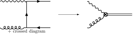
Figure 2: Feynman diagram for the QCD calculation (left) of the process $\gamma^{*}g\to c\bar{c}$ and for the amplitude calculation (right) by using the $[n]$-effective operators.

We now are ready to start with the calculation of the QCD amplitude. The process we are interested is shown in the left picture of the figure 2. The amplitude is given by:

$$\mathcal{A}(\gamma^{*}g\to c\bar{c}) =\frac{ige}{2}\epsilon_{\mu}(k_{1})\epsilon_{\nu}(k_{2})$$ (96)

$$\times\bar{u}(p)T^{a}\left[\frac{\gamma^{\mu}({p\!\!\!/}-{k\!\!\!/}_{1}+m_{c})\gamma^{\nu}}{k_{1}^{2}-2p\cdot k_{1}}+\frac{\gamma^{\nu}(-{\bar{p}\!\!\!/}+{k\!\!\!/}_{1}+m_{c})\gamma^{\mu}}{k_{1}^{2}-2\bar{p}\cdot k_{1}}\right]v(\bar{p})$$

$$=\frac{ige}{2}\epsilon_{\mu}(k_{1})\epsilon_{\nu}(k_{2})\left(\tilde{s}-\frac{4(\tilde{q}\cdot k_{1})^{2}}{\tilde{s}}\right)^{-1}\bar{u}(p)T^{a}\left[D^{\mu\nu}_{+}-\frac{2\,\tilde{q}\cdot k_{1}}{\tilde{s}}\,D^{\mu\nu}_{-}\right]v(\bar{p})\;,$$

where we have used that the gluon is on-shell $k_{2}^{2}=0$. Here, the center-of-mass energy is $s=(k_{1}+k_{2})^{2}$, which can be written as $s=P^{2}$ by momentum conservation, and we define $\tilde{s}$ as follows: $\tilde{s}\equiv(P^{2}-k_{1}^{2})/2$. Moreover, $e$ stands for the charge of the electron such that $e^{2}=4\pi\alpha$, with $\alpha$ the fine-structure constant in electrodynamics and $g^{2}=4\pi\alpha_{s}$ in QCD. The polarization vectors of the virtual photon and the incoming gluon are denoted by $\epsilon_{\mu}(k_{1})$ and $\epsilon_{\nu}(k_{2})$, respectively, while the quantities $D_{\pm}$ are defined as follows:

$$D^{\mu\nu}_{\pm} \equiv\gamma^{\mu}({p\!\!\!/}-{k\!\!\!/}_{1}+m_{c})\gamma^{\nu}\pm\gamma^{\nu}(-{\bar{p}\!\!\!/}+{k\!\!\!/}_{1}+m_{c})\gamma^{\mu}$$ (97)

$$=-({p\!\!\!/}-m_{c})\gamma^{\mu}\gamma^{\nu}\pm\gamma^{\nu}\gamma^{\mu}({\bar{p}\!\!\!/}+m_{c})+2(p\mp\bar{p})^{\mu}\gamma^{\nu}-(\gamma^{\mu}{k\!\!\!/}_{1}\gamma^{\nu}\mp\gamma^{\nu}{k\!\!\!/}_{1}\gamma^{\mu})\;.$$

We now use the Dirac equation, getting the following formula for the amplitude:

$$\mathcal{A}(\gamma^{*}g\to c\bar{c}) =\frac{ige}{2}\epsilon_{\mu}(k_{1})\epsilon_{\nu}(k_{2})\left(\tilde{s}-\frac{4(\tilde{q}\cdot k_{1})^{2}}{\tilde{s}}\right)^{-1}\left[\mathcal{D}_{+}^{\mu\nu,a}-\frac{2\,\tilde{q}\cdot k_{1}}{\tilde{s}}\,\mathcal{D}_{-}^{\mu\nu,a}\right]\;,$$ (98)

with

$$\mathcal{D}_{+}^{\mu\nu,a}\equiv\bar{u}(p)T^{a}D_{+}^{\mu\nu}v(\bar{p}) =\bar{u}(p)T^{a}\left[4\,\tilde{q}^{\mu}\gamma^{\nu}-\left(\gamma^{\mu}{k\!\!\!/}_{1}\gamma^{\nu}-\gamma^{\nu}{k\!\!\!/}_{1}\gamma^{\mu}\right)\right]v(\bar{p})\;,$$ (99)

$$\mathcal{D}_{-}^{\mu\nu,a}\equiv\bar{u}(p)T^{a}D_{-}^{\mu\nu}v(\bar{p}) =\bar{u}(p)T^{a}\left[2\,P^{\mu}\gamma^{\nu}-\left(\gamma^{\mu}{k\!\!\!/}_{1}\gamma^{\nu}+\gamma^{\nu}{k\!\!\!/}_{1}\gamma^{\mu}\right)\right]v(\bar{p})$$

$$=\bar{u}(p)T^{a}\left[2k_{2}^{\mu}\gamma^{\nu}-2k_{1}^{\nu}\gamma^{\mu}+2g^{\mu\nu}{k\!\!\!/}_{1}\right]v(\bar{p})\;.$$

Note that the Dirac structures in $\mathcal{D}_{\pm}$ determine the configuration of spin in which the heavy-quark pair is produced. In the boosted frame, described by the following relations: $\mathbf{p}+\bar{\mathbf{p}}=\mathbf{P}$ and $\mathbf{p}-\bar{\mathbf{p}}=2\mathbf{q}$, the heavy-quark spinors are the following:

$$u(p)=\frac{1}{\mathcal{N}}(2E_{q}+{P\!\!\!/}\gamma_{0})\begin{pmatrix}(E_{q}+m_{c})\,\xi\\ \mathbf{q}\cdot\boldsymbol{\sigma}\,\xi\end{pmatrix}\;,\quad v(\bar{p})=\frac{1}{\mathcal{N}}(2E_{q}+{P\!\!\!/}\gamma_{0})\begin{pmatrix}-\mathbf{q}\cdot\boldsymbol{\sigma}\,\eta\\ (E_{q}+m_{c})\,\eta\end{pmatrix}\;.$$ (100)

Here, $\mathcal{N}=\sqrt{4E_{q}(P^{0}+2E_{q})(E_{q}+m_{c})}$ and $\xi$ and $\eta$ are Pauli spinors. Taking the results from the appendix of Braaten:1996rp , we reduce the Dirac bilinears as a functions of Pauli spinors, Pauli matrices and relative momentum. Thus, we obtain the objects $\mathcal{D}_{\pm}$ as a combination of the spin-singlet and -triplet contributions described by the following spin factors: $\xi^{\dagger}T^{a}\eta$ and $\xi^{\dagger}T^{a}(\boldsymbol{\Lambda}\cdot\boldsymbol{\sigma})\eta$, respectively. As mentioned above, the angular momentum configuration will be described by the order in the $\mathbf{q}$-expansion. Then we expand the result obtained after using the expressions of Braaten:1996rp for the bilinears, getting the following expressions for $\mathcal{D}_{\pm}$ up to order $\mathbf{q}$:

$$\mathcal{D}_{+}^{\mu\nu,a} =i4m_{c}\epsilon^{ijk}\Lambda_{i}^{\mu}(\Lambda\cdot k_{1})_{j}\Lambda^{\nu}_{k}\,\xi^{\dagger}T^{a}\eta+\left[8m_{c}\tilde{q}^{\mu}g^{\nu\rho}+\frac{2k_{1,\beta}}{m_{c}}\left(g^{\nu\rho}(P^{\mu}\tilde{q}^{\beta}-P^{\beta}\tilde{q}^{\mu})\right.\right.$$ (101)

$$+\left.\left.g^{\mu\rho}(P^{\beta}\tilde{q}^{\nu}-P^{\nu}\tilde{q}^{\beta})+g^{\beta\rho}(P^{\nu}\tilde{q}^{\mu}-P^{\mu}\tilde{q}^{\nu})\right)\right]\xi^{\dagger}T^{a}\left(\boldsymbol{\Lambda}\cdot\boldsymbol{\sigma}\right)_{\rho}\eta\;,$$

$$\mathcal{D}_{-}^{\mu\nu,a} =4m_{c}\left(k_{2}^{\mu}g^{\nu\rho}-k_{1}^{\nu}g^{\mu\rho}+k_{1}^{\rho}g^{\mu\nu}\right)\xi^{\dagger}T^{a}\left(\boldsymbol{\Lambda}\cdot\boldsymbol{\sigma}\right)_{\rho}\eta\;.$$

From those equations, we see that the spin-singlet contribution comes from $\mathcal{D}_{+}$, whereas the spin-triplet contribution arises from a combination of $\mathcal{D}_{+}$ and $\mathcal{D}_{-}$. We now put these results in the amplitude and expand around $\mathbf{q}$:

$$\mathcal{A}(\gamma^{*}g\to c\bar{c}) =\frac{ige}{2}\epsilon_{\mu}(k_{1})\epsilon_{\nu}(k_{2})\frac{1}{\tilde{s}^{2}}\left[\tilde{s}\,\mathcal{D}_{+}^{\mu\nu,a}-2\,\tilde{q}\cdot k_{1}\mathcal{D}_{-}^{\mu\nu,a}\right]$$ (102)

$$=\frac{ige}{2}\epsilon_{\mu}(k_{1})\epsilon_{\nu}(k_{2})$$

$$\times\frac{1}{\tilde{s}^{2}}\left\{\tilde{s}\left[i2\,\epsilon^{\mu\nu\alpha\beta}k_{1,\alpha}P_{\beta}\right]\times\left(\xi^{\dagger}T^{a}\eta\right)\right.$$

$$\left.+4\left[\tilde{s}\,g^{\mu\rho}g^{\nu\sigma}\left(\frac{P^{2}+k_{1}^{2}}{2}\right)+\tilde{s}^{2}g^{\mu\sigma}g^{\nu\rho}-P^{2}\,k_{1}^{\sigma}k_{1}^{\rho}g^{\mu\nu}\right.\right.$$

$$\left.\left.+g^{\nu\rho}\left(\tilde{s}\,k_{1}^{\mu}k_{1}^{\sigma}-\frac{P^{2}+k_{1}^{2}}{2}k_{2}^{\mu}k_{1}^{\sigma}\right)-g^{\mu\rho}\left(\tilde{s}\,k_{2}^{\nu}k_{1}^{\sigma}-\frac{P^{2}+k_{1}^{2}}{2}k_{1}^{\nu}k_{1}^{\sigma}\right)\right.\right.$$

$$\left.\left.+\tilde{s}\left(g^{\mu\sigma}P^{\nu}k_{1}^{\rho}-g^{\nu\sigma}P^{\mu}k_{1}^{\rho}\right)\right]\times\left(\frac{(\boldsymbol{\Lambda}\cdot\mathbf{q})_{\sigma}}{M}\,\xi^{\dagger}T^{a}\left(\boldsymbol{\Lambda}\cdot\boldsymbol{\sigma}\right)_{\rho}\eta\right)\right\}\;,$$

where we have used that $\epsilon^{ijk}\Lambda_{i}^{\mu}\Lambda_{j}^{\alpha}\Lambda_{k}^{\nu}=\epsilon^{\beta\mu\alpha\nu}P_{\beta}/\sqrt{P^{2}}$. We have split the result into the S-state contribution, given by the third line of the last equation, and P-states contribution, given by the last three lines. Moreover, we would like to note a tricky aspect in eq. (102) (which is not relevant for the further discussion): since the boost matrices are defined as eq. (94), one can make the replacement $k_{1}^{\sigma(\rho)}\Lambda_{\sigma(\rho)}^{i}\leftrightarrow-k_{2}^{\sigma(\rho)}\Lambda_{\sigma(\rho)}^{i}$ in eq. (102), resulting in different consistent expressions of the matching tensor.

We now write the amplitude with the kinematics of the process in a photon frame considering mass corrections, which were established in section 2. Moreover, it is convenient to decompose the particles momenta by using the following vectors: $\kappa_{+}^{\mu}=\frac{P_{N}^{+}}{2}n^{\mu}$ and $\kappa_{-}^{\mu}=\frac{2}{P_{N}^{+}}\bar{n}^{\mu}$, such that $\kappa^{2}_{+}=\kappa^{2}_{-}=0$ and $\kappa_{+}\cdot\kappa_{+}=2$. Thus the virtual photon momentum reads:

$$k_{1}^{\mu}=\frac{-x_{B}P_{N}^{+}}{\gamma_{q}}\frac{n^{\mu}}{2}+\frac{Q^{2}\gamma_{q}}{x_{B}P_{N}^{+}}\frac{\bar{n}^{\mu}}{2}=\frac{-x_{B}}{\gamma_{q}}\kappa_{+}^{\mu}+\frac{Q^{2}\gamma_{q}}{4x_{B}}\kappa_{-}^{\mu}\;,$$ (103)

with $Q^{2}=-k_{1}^{2}$ and $\gamma_{q}$ denotes the mass corrections which is defined in eq. (7); note we choose a photon frame, so $Q_{\perp}=Q$ ($\mathbf{q}_{\perp}=\mathbf{k}_{1\perp}=0$) in the definition of $\gamma_{q}$. The Bjorken variable $x_{B}$ can be written in terms of the variable defined above, $\tilde{s}\equiv(P^{2}-k_{1}^{2})/2=(M^{2}+Q^{2})/2$:

$$x_{B}=\frac{Q^{2}}{2P_{N}\cdot k_{1}}=x_{S}\frac{Q^{2}}{2\,\tilde{s}}\;,$$ (104)

where $x_{S}$ is the collinear momentum fraction carried by the gluon from the proton which includes kinematic power corrections Scimemi:2019cmh . Thus the momenta involved in the amplitude above are the following:

$$k_{1}^{\mu} =\frac{-x_{S}Q^{2}}{\gamma_{q}\,\tilde{s}}\frac{\kappa_{+}^{\mu}}{2}+\frac{\gamma_{q}\,\tilde{s}}{x_{S}}\frac{\kappa_{-}^{\mu}}{2}\;,$$ (105)

$$k_{2}^{\mu} =x_{S}\kappa_{+}^{\mu}\;,$$

with $P^{\mu}=k_{1}^{\mu}+k_{2}^{\mu}$ by momentum conservation.

As mentioned in section 2, given that the effective $[n]$-operators in eq. (15) scale as $\lambda$, the effective amplitude scales as $\lambda$, so in order to perform the matching we need to expand the gluon polarization vector to order $\lambda$:

$$\epsilon_{\nu}=\epsilon_{\perp\nu}-\frac{k_{2\perp\nu}}{\bar{n}\cdot k_{2}}\bar{n}\cdot\epsilon\;.$$ (106)

Therefore, inserting eq. (105) and eq. (106) into eq. (102) yields:

$$\mathcal{A}(\gamma^{*}g\to c\bar{c}) =\frac{ige}{2}\epsilon_{\mu}(k_{1})\,\epsilon_{\perp\nu}(k_{2})$$ (107)

$$\times\left\{\frac{\gamma_{q}}{2}i2\,\epsilon^{\mu\nu\alpha\beta}\kappa_{-\alpha}\kappa_{+\beta}\times\left(\xi^{\dagger}T^{a}\eta\right)\right.$$

$$\left.+4\left[g_{\perp}^{\nu\sigma}\left(g^{\mu\rho}\frac{M^{2}-Q^{2}}{M^{2}+Q^{2}}+\frac{x_{S}^{2}}{M^{2}+Q^{2}}\left(1-\frac{2\,x_{S}Q^{2}}{\gamma_{q}(M^{2}+Q^{2})}\right)\kappa_{+}^{\mu}\kappa_{+}^{\rho}+\frac{\gamma_{q}}{2}\,\kappa_{-}^{\mu}\kappa_{+}^{\rho}\right)\right.\right.$$

$$\left.\left.+g_{\perp}^{\nu\rho}\left(g^{\mu\sigma}+\frac{2x_{S}^{2}}{(M^{2}+Q^{2})^{2}}\left(M^{2}+Q^{2}\frac{1-\gamma_{q}}{\gamma_{q}}\right)\kappa_{+}^{\mu}\kappa_{+}^{\sigma}-\frac{\gamma_{q}}{2}\kappa_{-}^{\mu}\kappa_{+}^{\sigma}\right)\right.\right.$$

$$\left.\left.-g^{\nu\mu}_{\perp}\frac{4\,x_{S}^{2}M^{2}}{(M^{2}+Q^{2})^{2}}\,\kappa_{+}^{\sigma}\kappa_{+}^{\rho}\right]\times\left(\frac{(\boldsymbol{\Lambda}\cdot\mathbf{q})_{\sigma}}{M}\,\xi^{\dagger}T^{a}\left(\boldsymbol{\Lambda}\cdot\boldsymbol{\sigma}\right)_{\rho}\eta\right)\right\}\;,$$

with $k_{2\perp\nu}=0$. In the light-cone basis, built by $n$ and $\bar{n}$, the amplitude is given by:

$$\mathcal{A}(\gamma^{*}g\to c\bar{c}) =\frac{ige}{2}\epsilon_{\mu}(k_{1})\,\epsilon_{\perp\nu}(k_{2})$$ (108)

$$\times \left\{-i4\,\epsilon^{\mu\nu}_{\perp}\frac{\gamma_{q}}{2}\times\left(\xi^{\dagger}T^{a}\eta\right)\right.$$

$$+ \,4\left.\left[g_{\perp}^{\nu\sigma}\left(g^{\mu\rho}\frac{M^{2}-Q^{2}}{M^{2}+Q^{2}}+\frac{x_{S}^{2}P_{N}^{+2}}{4(M^{2}+Q^{2})}\left(1-\frac{2\,x_{S}Q^{2}}{\gamma_{q}(M^{2}+Q^{2})}\right)n^{\mu}n^{\rho}+\frac{\gamma_{q}}{2}\,\bar{n}^{\mu}n^{\rho}\right)\right.\right.$$

$$+ \left.\left.g_{\perp}^{\nu\rho}\left(g^{\mu\sigma}+\frac{x_{S}^{2}P_{N}^{+2}}{2(M^{2}+Q^{2})^{2}}\left(M^{2}+Q^{2}\frac{1-\gamma_{q}}{\gamma_{q}}\right)n^{\mu}n^{\sigma}-\frac{\gamma_{q}}{2}\bar{n}^{\mu}n^{\sigma}\right)\right.\right.$$

$$- \left.\left.g^{\nu\mu}_{\perp}\frac{x_{S}^{2}P_{N}^{+2}M^{2}}{(M^{2}+Q^{2})^{2}}\,n^{\sigma}n^{\rho}\right]\times\left(\frac{(\boldsymbol{\Lambda}\cdot\mathbf{q})_{\sigma}}{M}\,\xi^{\dagger}T^{a}\left(\boldsymbol{\Lambda}\cdot\boldsymbol{\sigma}\right)_{\rho}\eta\right)\right\}\;,$$

with $\epsilon_{\perp}^{\mu\nu}=\tensor{\epsilon}{{}^{\mu}{}^{\nu}_{\alpha}{}_{\beta}}\bar{n}^{\alpha}n^{\beta}/2$ and $g_{\perp}^{\mu\nu}=g^{\mu\nu}-(n^{\mu}\bar{n}^{\nu}+\bar{n}^{\mu}n^{\nu})/2$. For easy comparison with the effective-theory side of the matching equation, we rewrite this result as follows:

$$\mathcal{A}(\gamma^{*}g\to c\bar{c})=\epsilon_{\mu}(k_{1})\left(\mathcal{A}_{{}^{1}S_{0}^{[8]}}^{\mu}+\mathcal{A}_{{}^{3}P_{J}^{[8]}}^{\mu}\right)\;,$$ (109)

with

$$\mathcal{A}_{{}^{1}S_{0}^{[8]}}^{\mu} =2\,ge\,\epsilon_{\perp}^{\mu\nu}\frac{\gamma_{q}}{2}\,\epsilon_{\perp\nu}(k_{2})\times\left(\xi^{\dagger}T^{a}\eta\right)\;,$$ (110)

$$\mathcal{A}_{{}^{3}P_{J}^{[8]}}^{\mu} =i2\,ge\left\{g_{\perp}^{\nu\sigma}\left[g^{\mu\rho}\frac{M^{2}-Q^{2}}{M^{2}+Q^{2}}+\frac{x_{S}^{2}P_{N}^{+2}}{4(M^{2}+Q^{2})}\left(1-\frac{2\,x_{S}Q^{2}}{\gamma_{q}(M^{2}+Q^{2})}\right)n^{\mu}n^{\rho}+\frac{\gamma_{q}}{2}\,\bar{n}^{\mu}n^{\rho}\right]\right.$$

$$+g_{\perp}^{\nu\rho}\left[\left.g^{\mu\sigma}+\frac{x_{S}^{2}P_{N}^{+2}}{2(M^{2}+Q^{2})^{2}}\left(M^{2}+Q^{2}\frac{1-\gamma_{q}}{\gamma_{q}}\right)n^{\mu}n^{\sigma}-\frac{\gamma_{q}}{2}\bar{n}^{\mu}n^{\sigma}\right]\right.$$

$$\left.-g^{\nu\mu}_{\perp}\frac{x_{S}^{2}P_{N}^{+2}M^{2}}{(M^{2}+Q^{2})^{2}}\,n^{\sigma}n^{\rho}\right\}\times\left(\epsilon_{\perp\nu}-\frac{k_{2\perp\nu}}{\bar{n}\cdot k_{2}}\bar{n}\cdot\epsilon\right)\times\left(\frac{(\boldsymbol{\Lambda}\cdot\mathbf{q})_{\sigma}}{M}\,\xi^{\dagger}T^{a}\left(\boldsymbol{\Lambda}\cdot\boldsymbol{\sigma}\right)_{\rho}\eta\right)\;.$$

We now use that the product $q^{i}\sigma^{j}$ can be decomposed into the following three tensors:

$$q^{i}\sigma^{j}=\frac{\delta^{ij}}{3}\mathbf{q}\cdot\boldsymbol{\sigma}+\frac{\epsilon^{ijk}}{2}(\mathbf{q}\times\boldsymbol{\sigma})^{k}+q^{(i}\sigma^{j)}\;,$$ (111)

with $q^{(i}\sigma^{j)}=(q^{i}\sigma^{j}+q^{j}\sigma^{i})/2-\mathbf{q}\cdot\boldsymbol{\sigma}\delta^{ij}/3$. We obtain the tesnorial structures for $J=0,1,2$ from this decomposition. In fact, the scalar term is describing the state $J=0$, the vector one is describing the state $J=1$ and the symmetric-traceless one is describing the state $J=2$. Thus we apply (111) to the P-wave contribution of the QCD amplitude (110):

$$\mathcal{A}^{\mu}_{{}^{3}P_{0}^{[8]}} =\Gamma^{\mu\nu\sigma\rho}\left(-g_{\sigma\rho}+\frac{P_{\sigma}P_{\rho}}{P^{2}}\right)\,\epsilon_{\perp\nu}\times\frac{1}{3}\left(\xi^{\dagger}_{\mathbf{q}}(\mathbf{q}\cdot\boldsymbol{\sigma})\,T^{a}\eta_{-\mathbf{q}}\right)\;,$$ (112)

$$\mathcal{A}^{\mu}_{{}^{3}P_{1}^{[8]}} =\Gamma^{\mu\nu\sigma\rho}\epsilon_{\alpha\beta\sigma\rho}\Lambda^{\alpha}_{k}\frac{P^{\beta}}{M}\,\epsilon_{\perp\nu}\times\frac{1}{2}\left(\xi^{\dagger}_{\mathbf{q}}(\mathbf{q}\times\boldsymbol{\sigma})^{k}\,T^{a}\eta_{-\mathbf{q}}\right)\;,$$

$$\mathcal{A}^{\mu}_{{}^{3}P_{2}^{[8]}} =\Gamma^{\mu\nu\sigma\rho}\Lambda^{i}_{\sigma}\Lambda^{j}_{\rho}\,\epsilon_{\perp\nu}\times\left(\xi^{\dagger}_{\mathbf{q}}\,(q_{(i}\sigma_{j)})\,T^{a}\eta_{-\mathbf{q}}\right)\;,$$

where we have used that $\Lambda^{\alpha}_{i}\Lambda^{\beta}_{i}=-g^{\alpha\beta}+P^{\alpha}P^{\beta}/P^{2}$ and $\epsilon^{ijk}\Lambda_{j}^{\alpha}\Lambda_{k}^{\beta}=\epsilon^{\mu\nu\alpha\beta}\Lambda_{\mu}^{i}P_{\nu}/\sqrt{P^{2}}$ and the tensor $\Gamma^{\mu\nu\sigma\rho}$ is defined as:

$$\Gamma^{\mu\nu\sigma\rho} =\frac{i2ge}{M}\left\{g_{\perp}^{\nu\sigma}\left[g^{\mu\rho}\frac{M^{2}-Q^{2}}{M^{2}+Q^{2}}+\frac{M^{2}+Q^{2}}{4Q^{4}}x_{B}^{2}P_{N}^{+2}\left(1-\frac{2x_{B}}{\gamma_{q}}\right)n^{\mu}n^{\rho}+\frac{\gamma_{q}}{2}\bar{n}^{\mu}n^{\rho}\right]\right.$$ (113)

$$+g_{\perp}^{\nu\rho} \left.\left[g^{\mu\sigma}+\frac{x_{B}^{2}P_{N}^{+2}}{2Q^{4}}\left(M^{2}+Q^{2}\frac{(1-\gamma_{q})}{\gamma_{q}}\right)n^{\mu}n^{\sigma}-\frac{\gamma_{q}}{2}\bar{n}^{\mu}n^{\sigma}\right]-g_{\perp}^{\nu\mu}\frac{x_{B}^{2}P_{N}^{+2}M^{2}}{Q^{4}}n^{\sigma}n^{\rho}\right\}\;.$$

where we use that $x_{S}=x_{B}(M^{2}+Q^{2})/Q^{2}$.

So far, we have calculated the amplitude for the S and P -states in the nonrelativistic limit of QCD. To obtain the matching tensors, we need to deal with the calculation of the amplitude by using the $[n]$-operators defined in eq. (22). Note that the expansion of the gluon building block of SCET can be written in terms of gluon fields as follows:

$$\mathcal{B}_{n\perp}^{\mu}=A_{n\perp}^{\mu}-\frac{k_{2\perp}^{\mu}}{\bar{n}\cdot q}\bar{n}\cdot A_{n,k_{2}}+\ldots\;,$$ (114)

where the dots denote terms with more collinear gluon fields, i.e., higher orders in the $\lambda$-expansion. Since the components of the collinear gluon field scales in the same way as the components of the collinear momentum, the transverse component of a collinear gluon field $A_{n\perp}$ scales as $\lambda$. In addition, we can see from the vNRQCD Lagrangian that the heavy-quark fields scale as $\lambda^{0}$. Thus the effective $[n]$-operators scale as $\lambda$. Therefore, since we have expanded the QCD amplitude up to order $\lambda$, we are able to do the matching between both sides. The effective amplitude is given by:

$$\mathcal{A}^{\mu,\text{eff}} =\mathcal{A}^{\mu,\text{eff}}_{{}^{1}S_{0}^{[8]}}+\mathcal{A}^{\mu,\text{eff}}_{{}^{3}P_{0}^{[8]}}+\mathcal{A}^{\mu,\text{eff}}_{{}^{3}P_{1}^{[8]}}\;+\mathcal{A}^{\mu,\text{eff}}_{{}^{3}P_{2}^{[8]}}\;,$$ (115)

with

$$\mathcal{A}^{\mu,\text{eff}}_{{}^{1}S_{0}^{[8]}} =\Gamma^{\mu\nu}_{{}^{1}S_{0}^{[8]}}\left<c\bar{c}\right|\psi^{\dagger}_{\mathbf{p}}\left(A_{n\perp\nu}-\frac{k_{2\perp\nu}}{\bar{n}\cdot k_{2}}\bar{n}\cdot A_{n,k_{2}}\right)\chi_{\bar{\mathbf{p}}}\left|g\right>$$ (116)

$$=M\,\Gamma^{\mu\nu}_{{}^{1}S_{0}^{[8]}}\,\epsilon_{\perp\nu}\times\left(\xi_{\mathbf{p}}^{\dagger}T^{a}\eta_{\bar{\mathbf{p}}}\right)\;,$$

$$\mathcal{A}^{\mu,\text{eff}}_{{}^{3}P_{0}^{[8]}} =M\,\Gamma_{{}^{3}P_{0}^{[8]}}^{\mu\nu}\,\epsilon_{\perp\nu}\times\left(\frac{1}{M}\,\xi^{\dagger}_{\mathbf{p}}\,\left(\mathbf{q}\cdot\boldsymbol{\sigma}\right)\,T^{a}\eta_{\bar{\mathbf{p}}}\right)\;,$$

$$\mathcal{A}^{\mu,\text{eff}}_{{}^{3}P_{1}^{[8]}} =M\,\Gamma_{{}^{3}P_{1}^{[8]}}^{\mu\nu,k}\,\epsilon_{\perp\nu}\times\left(\frac{1}{M}\,\xi^{\dagger}_{\mathbf{p}}\,\left(\mathbf{q}\times\boldsymbol{\sigma}\right)^{k}\,T^{a}\eta_{\bar{\mathbf{p}}}\right)\;,$$

$$\mathcal{A}^{\mu,\text{eff}}_{{}^{3}P_{2}^{[8]}} =M\,\Gamma_{{}^{3}P_{2}^{[8]}}^{\mu\nu,ij}\,\epsilon_{\perp\nu}\times\left(\frac{1}{M}\,\xi^{\dagger}_{\mathbf{p}}\,\left(q^{(i}\sigma^{j)}\right)\,T^{a}\eta_{\bar{\mathbf{p}}}\right)\;.$$

where we have used that $k_{2\perp}^{\nu}=0$, $\left<c\bar{c}\right|\psi^{\dagger}\chi\left|0\right>=M\,\xi^{\dagger}\eta$ in perturbative NRQCD. Equating the QCD amplitude (108) with the effective amplitude (115), we obtain the ${}^{1}S_{0}^{[8]}$ and ${}^{3}P_{J=0,1,2}^{[8]}$ matching tensors:

$$\Gamma^{\mu\nu}_{{}^{3}P_{0}^{[8]}} =-\frac{i2\,ge}{3M}\left(\frac{M^{2}(\gamma_{q}^{2}+2)+Q^{2}\gamma_{q}^{2}}{M^{2}+Q^{2}}\right)g_{\perp}^{\mu\nu}\;,$$ (117)

$$\Gamma^{\mu\nu,k}_{{}^{3}P_{1}^{[8]}} =\frac{i\,ge}{M}\left(\frac{x_{B}^{2}P_{N}^{+2}\left(M^{2}\gamma_{q}+Q^{2}\left(\gamma_{q}-1\right)\right)(n\cdot\Lambda)_{k}-\gamma_{q}^{2}Q^{4}(\bar{n}\cdot\Lambda)_{k}}{\gamma_{q}x_{B}P_{N}^{+}M\left(M^{2}+Q^{2}\right)}\right)\epsilon_{\perp}^{\mu\nu}\;,$$

$$\Gamma^{\mu\nu,ij}_{{}^{3}P_{2}^{[8]}} =-\frac{i2\,ge}{M}\left(\frac{x_{B}^{2}P_{N}^{+2}M^{2}}{Q^{4}}\right)(n\cdot\Lambda)_{i}(n\cdot\Lambda)_{j}\,g_{\perp}^{\mu\nu}\;,$$

with

$$(n\cdot\Lambda)^{i}=\delta^{3i}+P^{i}\left(\frac{1}{2M}+\frac{1}{P^{3}}\left(\frac{P^{0}}{M}-1\right)\right)\;,$$ (118)

$$(\bar{n}\cdot\Lambda)^{i}=-\delta^{3i}+P^{i}\left(\frac{1}{2M}-\frac{1}{P^{3}}\left(\frac{P^{0}}{M}-1\right)\right)\;.$$

Considering that $n^{\mu}=(1,0,0,1)$ and $\bar{n}^{\mu}=(1,0,0,-1)$, we can write $P^{0}$ and $P^{3}$ as follows:

$$P^{0} =\frac{x_{B}P_{N}^{+}}{2}\left(\frac{M^{2}+Q^{2}}{Q^{2}}-\frac{1}{\gamma_{q}}\right)+\frac{\gamma_{q}Q^{2}}{2x_{B}P_{N}^{+}}\;,$$ (119)

$$P^{3} =\frac{x_{B}P_{N}^{+}}{2}\left(\frac{M^{2}+Q^{2}}{Q^{2}}-\frac{1}{\gamma_{q}}\right)-\frac{\gamma_{q}Q^{2}}{2x_{B}P_{N}^{+}}\;.$$

Appendix C Details of the calculation

In this section, we compute the ${}^{1}S_{0}^{[8]}$ LDME and TMDShF at NLO in the vNRQCD framework, which is defined in appendix A. Given the close similarity in the computation of the P-wave contributions, we have delineated the distinctions in appendix D compared to the present section.

C.1 NLO calculation of the TMDShF

Figure 3: Diagrams showing the LO and the Coulomb interaction. Hermitian conjugate of right diagram is not shown.

Figure 4: Diagrams showing the ultrasoft gluon exchanges between heavy quarks and (anti)quarks contributing to NLO. Hermitian conjugates of diagrams a and c are not shown. The soft and ultrasoft Wilson lines are not shown.

From Bodwin:1994jh , we know that the operator for state ${}^{1}S_{0}^{[8]}$, in terms of the heavy-quark annihilation field $\psi$ and the heavy-antiquark creation field $\chi$, is as follows

$$\mathcal{O}_{8}\left({}^{1}S_{0}\right)=\chi^{\dagger}T^{a}\psi\,\mathcal{N}_{\psi}\,\psi^{\dagger}T^{a}\chi\;,$$ (120)

where $\mathcal{N}_{\psi}\equiv a_{\psi}^{\dagger}a_{\psi}$ is defined above as the number operator for the state $J/\psi$. Consequently, the ${}^{1}S_{0}^{[8]}$ LDME will be the vacuum expectation value of that operator. From the figures presented in this appendix, it can be seen how the LDME can be illustrated as a crossed circle and two quark lines. The crossed circle represents the state in which the heavy-quark pair is produced or decays through the bilinear formed by the fields and the color and angular momentum structure, e.g., for the state we are concerned with, the left crossed circle will be $\psi^{\dagger}T^{a}\chi$. In particular, in the figure 3 and figure 4 the Feynman diagrams for the LDME NLO contribution are shown.

At LO, the ${}^{1}S_{0}^{[8]}$ LDME looks like this

$$\left<0|\mathcal{O}_{8}(^{1}S_{0})|0\right>^{\text{LO}}\equiv\left<{}^{1}S_{0}^{[8]}\right>^{\text{LO}}=M^{2}\,\eta^{\dagger}T^{a}\xi\times\xi^{\dagger}T^{a}\eta\;.$$ (121)

Here $\eta$ and $\xi$ are the Pauli 2-component spinors. The Dirac 4-component spinors $u(p)$ and $v(\bar{p})$ are defined in terms of the Pauli spinors in the standard nonrelativistic form (see eq. (100), where we explicitly show the relation between both). Expanding the Dirac spinors in the velocity in perturbative NRQCD, one finds $\left<c\bar{c}\right|\psi^{\dagger}\chi\left|0\right>=M\xi^{\dagger}\eta$, with $M$ the mass of the heavy-quark state, and where we have implicitly summed over the helicity of the bound state.

The diagrams which contribute to the NLO are called Coulomb interaction and chromo-electric dipole transition. The Coulomb interaction contribution arises from the term of the second line term of vNRQCD interaction Lagrangian in eq. (92):

$$\mathcal{L}_{\text{vNRQCD}}^{\text{Coul.}}=\sum_{\mathbf{p},\mathbf{p}^{\prime}}\frac{4\pi\alpha_{s}}{(\mathbf{p}-\mathbf{p}^{\prime})^{2}}\,\psi_{\mathbf{p}}^{\dagger}T^{a}\psi_{\mathbf{p}^{\prime}}\,\chi_{-\mathbf{p}}^{\dagger}\bar{T}^{a}\chi_{-\mathbf{p}^{\prime}}\;.$$ (122)

The leading order Lagrangian gives the intermediate fermion propagator for the below equation $p^{0}+k^{0}-(\mathbf{p}+\mathbf{k})^{2}/2m$. Additionally, considering that $\mathbf{p}-\mathbf{p}^{\prime}=\mathbf{k}$, we obtain

$$\left<{}^{1}S_{0}^{[8]}\right>^{\text{Coul.}} =\left<{}^{1}S_{0}^{[8]}\right>^{\text{LO}}(-i4\pi\alpha_{s})\left(C_{F}-C_{A}/2\right)\int\frac{d^{4}k}{(2\pi)^{4}}\frac{1}{\mathbf{k}^{2}}\frac{1}{[p^{0}+k^{0}-(\mathbf{p}+\mathbf{k})^{2}/2m+i\epsilon]}$$ (123)

$$\times\frac{1}{[p^{0}-k^{0}-(\mathbf{p}+\mathbf{k})^{2}/2m+i\epsilon]}+h.c.\;.$$

Here we compute the integral on $k^{0}$ by contour integration, i.e., closing the contour in the lower half of the complex plane and picking up the pole $k^{0}=-p^{0}+(\mathbf{p}+\mathbf{k})^{2}/2m-i\epsilon$. We find that the contribution reduces to the following integral on the three-momentum:

$$\left<{}^{1}S_{0}^{[8]}\right>^{\text{Coul.}} =\left<{}^{1}S_{0}^{[8]}\right>^{\text{LO}}(4\pi\alpha_{s}m_{c})\left(C_{F}-C_{A}/2\right)\int\frac{d^{3}k}{(2\pi)^{3}}\frac{1}{\mathbf{k}^{2}}\frac{1}{\mathbf{k}^{2}+2\mathbf{p}\cdot\mathbf{k}-i\epsilon}+h.c.$$ (124)

$$=\left<{}^{1}S_{0}^{[8]}\right>^{\text{LO}}\left(C_{F}-C_{A}/2\right)\frac{\pi\alpha_{s}}{2\text{v}}\;,$$

where we have used that $\mathbf{v}=\mathbf{p}/m_{c}$ and $\text{v}=|\mathbf{v}|$.

The chromo-electric effect contribution arises from the term of the first line of the vNRQCD interaction Lagrangian:

$$\mathcal{L}_{\text{vNRQCD}}^{\text{Chro.}}=-g\sum_{\mathbf{p}}\psi_{\mathbf{p}}^{\dagger}\left(\frac{\mathbf{B}_{us}\cdot\mathbf{P}}{m_{c}}\right)\psi_{\mathbf{p}}(x)+(\psi\rightarrow\chi,\,T\to\bar{T})\;.$$ (125)

Let us look at this term in more detail. As mentioned before, after BPS redefinition in eq. (90), the usoft Wilson lines arise. In the rest of the paper, we assume they are implicit in the soft Wilson lines but here we need write explicitly (at NLO):

$$Y_{v}(x) =1-ig\int_{-\infty}^{0}dt^{\prime}A_{us}^{0}(t+t^{\prime},\mathbf{x})+\mathcal{O}(g^{2})$$ (126)

$$=1+\int\frac{d^{d}k}{(2\pi)^{d}}e^{-ik\cdot x}\left(\frac{g\,T^{a}}{k^{0}}\right)A_{us}^{0,a}(k)+\mathcal{O}(g^{2})\;,$$

where we use that $v=(1,\mathbf{0})$ in the rest frame of the $J/\psi$. Inserting the expanded usoft Wilson line (126) in eq. (125) through the product $\mathbf{B}_{us}\cdot\mathbf{P}$, we obtain

$$\mathbf{B}_{us}\cdot\mathbf{P} =\left(\frac{-1}{g}Y_{u}^{\dagger}(iD^{i})Y_{u}\right)P^{i}$$ (127)

$$=\int\frac{d^{d}k}{(2\pi)^{d}}e^{-ik\cdot x}\left(\mathbf{A}_{us}\cdot\mathbf{P}-\frac{A_{us}^{0}}{k^{0}}\mathbf{k}\cdot\mathbf{P}\right)\;,$$

and consequently, the chromo-electric term in the Lagrangian is given by

$$\mathcal{L}_{\text{vNRQCD}}^{\text{Chro.}} =\frac{-g}{m_{c}}\sum_{\mathbf{p}}\int\frac{d^{d}k}{(2\pi)^{d}}e^{-ik\cdot x}\psi^{\dagger}_{\mathbf{p}}\left(\mathbf{A}_{us}\cdot\mathbf{p}-\frac{A_{us}^{0}}{k^{0}}\mathbf{k}\cdot\mathbf{p}\right)\psi_{\mathbf{p}}+(\psi\rightarrow\chi,\,T\to\bar{T})\;.$$ (128)

Here we act with the label momentum operator on the heavy-(anti)quark fields as follows $\mathbf{P}\,\psi_{\mathbf{p}}=\mathbf{p}\,\psi_{\mathbf{p}}$. From this form of the interaction term, the loop integral reads (e.g., here we show the contribution of the figure 4b)

$$\left<{}^{1}S_{0}^{[8]}\right>^{\ref{fig:TMDShF-ChroElectric}\text{b}} =\frac{4\pi\alpha_{s}}{m_{c}^{2}}\,I^{\ref{fig:TMDShF-ChroElectric}\text{b}}\eta^{\dagger}T^{a}T^{b}\xi\times\xi^{\dagger}T^{b}T^{a}\eta\;,$$ (129)

with

$$I^{\ref{fig:TMDShF-ChroElectric}\text{b}} =i\mu^{2\varepsilon}\int\frac{d^{d}k}{(2\pi)^{d}}\frac{\mathbf{p}^{2}-(\mathbf{p}\cdot\mathbf{k})^{2}/\mathbf{k}^{2}}{(k^{0})^{2}-\mathbf{k}^{2}+i\epsilon}\,\frac{1}{[p^{0}-k^{0}-(\mathbf{p}+\mathbf{k})^{2}/2m]^{2}}$$ (130)

$$=\mu^{2\varepsilon}\int\frac{d^{3-2\varepsilon}\mathbf{k}}{(2\pi)^{3-2\varepsilon}}\frac{\mathbf{p}^{2}-(\mathbf{p}\cdot\mathbf{k})^{2}/\mathbf{k}^{2}}{2|\mathbf{k}|}\frac{1}{-|\mathbf{k}|}\,\frac{1}{-|\mathbf{k}|}$$

$$=\mu^{2\varepsilon}\frac{1}{2}\int\frac{d^{3-2\varepsilon}\mathbf{k}}{(2\pi)^{3-2\varepsilon}}\frac{\mathbf{p}^{2}-(\mathbf{p}\cdot\mathbf{k})^{2}/\mathbf{k}^{2}}{|\mathbf{k}|^{3}}=\frac{1}{2}\frac{\mathbf{p}^{2}}{6\pi^{2}}\left(\frac{1}{\varepsilon_{\rm{UV}}}-\frac{1}{\varepsilon_{\rm{IR}}}\right)\;.$$

In the second equality we have computed the contour-integral over $k^{0}$ around the pole $k^{0}=|\mathbf{k}|-i\epsilon$ and in the third equality we have expanded the integrand in powers of $\mathbf{p}/m_{c}$ and $\mathbf{k}/m_{c}$. To do so we need the following integral:

$$\mu^{2\varepsilon}\int d^{3-2\varepsilon}\mathbf{k}\,\frac{1}{|\mathbf{k}|^{3}} =2\pi\left(\frac{1}{\varepsilon_{\rm{UV}}}-\frac{1}{\varepsilon_{\rm{IR}}}\right)\;.$$ (131)

Diagrams figure 4c,d give the same contribution as (129), but the color configuration of the spin factor changes as follows

$$\left<{}^{1}S_{0}^{[8]}\right>^{\ref{fig:TMDShF-ChroElectric}\text{c}} =\left<{}^{1}S_{0}^{[8]}\right>^{\ref{fig:TMDShF-ChroElectric}\text{b}}\left(T^{a}T^{b}\otimes T^{b}T^{a}\rightarrow T^{a}T^{b}\otimes T^{a}T^{b}\right)\;,$$ (132)

$$\left<{}^{1}S_{0}^{[8]}\right>^{\ref{fig:TMDShF-ChroElectric}\text{c}^{*}} =\left<{}^{1}S_{0}^{[8]}\right>^{\ref{fig:TMDShF-ChroElectric}\text{b}}\left(T^{a}T^{b}\otimes T^{b}T^{a}\rightarrow T^{b}T^{a}\otimes T^{b}T^{a}\right)\;,$$

$$\left<{}^{1}S_{0}^{[8]}\right>^{\ref{fig:TMDShF-ChroElectric}\text{d}} =\left<{}^{1}S_{0}^{[8]}\right>^{\ref{fig:TMDShF-ChroElectric}\text{b}}\left(T^{a}T^{b}\otimes T^{b}T^{a}\rightarrow T^{b}T^{a}\otimes T^{a}T^{b}\right)\;.$$

Using the following relations

$$T^{a}T^{b}\otimes T^{b}T^{a} =\frac{C_{F}}{2N_{c}}\,1\otimes 1+\frac{N_{c}^{2}-2}{2N_{c}}\,T^{a}\otimes T^{a}\;,$$ (133)

$$T^{a}T^{b}\otimes T^{a}T^{b} =\frac{C_{F}}{2N_{c}}\,1\otimes 1-\frac{1}{N_{c}}\,T^{a}\otimes T^{a}\,,$$

and summing the contribution of all diagrams, we obtain the following

$$\left<{}^{1}S_{0}^{[8]}\right>^{\ref{fig:TMDShF-ChroElectric}\text{b,c,d}} =\frac{4\alpha_{s}}{3\pi m_{c}^{2}}\left(C_{F}\frac{1\otimes 1}{2N_{c}}+B_{F}\,T^{a}\otimes T^{a}\right)\eta^{\dagger}p^{k}\xi\times\xi^{\dagger}p^{k}\eta\left(\frac{1}{\varepsilon_{\rm{UV}}}-\frac{1}{\varepsilon_{\rm{IR}}}\right)\;,$$ (134)

where $B_{F}=(N_{c}^{2}-4)/4N_{c}$. Here we do not consider the virtual diagram (figure 4a) because it gives a contribution at higher order in the relative velocity expansion:

$$\left<{}^{1}S_{0}^{[8]}\right>^{\ref{fig:TMDShF-ChroElectric}\text{a}}\propto\frac{\mathbf{p}^{2}}{m_{c}^{2}}\,\eta^{\dagger}T^{b}T^{a}T^{b}\xi\times\xi^{\dagger}T^{a}\eta=\frac{\mathbf{p}^{2}}{m_{c}^{2}}(C_{F}-C_{A}/2)\eta^{\dagger}T^{a}\xi\times\xi^{\dagger}T^{a}\eta\;.$$ (135)

Therefore the following result is the contribution for the ${}^{1}S_{0}^{[8]}$ LDME of the usoft gluon exchange between heavy-quarks and (anti)quarks at leading order on v

$$\left<{}^{1}S_{0}^{[8]}\right>^{\ref{fig:TMDShF-ChroElectric}} =\frac{4\alpha_{s}}{3\pi m_{c}^{2}}\left(C_{F}\left<{}^{1}P_{1}^{[1]}\right>^{\text{LO}}+B_{F}\left<{}^{1}P_{1}^{[8]}\right>^{\text{LO}}\right)\left(\frac{1}{\varepsilon_{\rm{UV}}}-\frac{1}{\varepsilon_{\rm{IR}}}\right)\;.$$ (136)

We put together the previous results and conclude that the ${}^{1}S_{0}^{[8]}$ LDME at NLO is the following

$$\left<{}^{1}S_{0}^{[8]}\right>^{\text{NLO}} =\left<{}^{1}S_{0}^{[8]}\right>^{\ref{fig:TMDShF-LOandCoulomb}\text{LO}}+\left<{}^{1}S_{0}^{[8]}\right>^{\ref{fig:TMDShF-LOandCoulomb}\text{Coul.}}+\left<{}^{1}S_{0}^{[8]}\right>^{\ref{fig:TMDShF-ChroElectric}}$$ (137)

$$=\left(1+\left(C_{F}-C_{A}/2\right)\frac{\pi\alpha_{s}}{2\text{v}}\right)\left<{}^{1}S_{0}^{[8]}\right>^{\text{LO}}$$

$$+\frac{4\alpha_{s}}{3\pi m_{c}^{2}}\left(C_{F}\left<{}^{1}P_{1}^{[1]}\right>^{\text{LO}}+B_{F}\left<{}^{1}P_{1}^{[8]}\right>^{\text{LO}}\right)\left(\frac{1}{\varepsilon_{\rm{UV}}}-\frac{1}{\varepsilon_{\rm{IR}}}\right)\;.$$

C.2 NLO calculation of the LDME

We proceed to calculate the ${}^{1}S_{0}^{[8]}$ TMD shape function in eq. (38) at NLO. In addition to the Coulomb interaction and chromo-electric transition, there are three additional contributions arising from the Wilson lines in the definition of the TMDShF. The Feynman diagrams illustrating these interactions are depicted in figure 5, figure 6 and figure 7. As previously mentioned, due to rapidity divergences arising from one of the Wilson lines (the one in the $n$ collinear direction) in the TMDShF, we employ the delta rapidity regulator at the operator level in the Wilson lines definition (16). For clarity, we opt to modify the notation for the shape functions in this subsection, replacing $S_{[n]\to J/\psi}$ to $S_{[n]}$, with the understanding that the final state is the $J/\psi$.

From the previous results in eq. (121) and eq. (124), it is straightforward to deduce that

$$S_{{}^{1}S_{0}^{[8]}}^{\ref{fig:TMDShF-LOandCoulomb}\text{LO}}(\mathbf{k}_{\perp}) =\delta^{2}(\mathbf{k}_{\perp})\left<{}^{1}S_{0}^{[8]}\right>^{\text{LO}}\;,$$ (138)

$$S_{{}^{1}S_{0}^{[8]}}^{\ref{fig:TMDShF-LOandCoulomb}\text{Coul.}}(\mathbf{k}_{\perp}) =\delta^{2}(\mathbf{k}_{\perp})\left(C_{F}-C_{A}/2\right)\frac{\pi\alpha_{s}}{2\text{v}}\left<{}^{1}S_{0}^{[8]}\right>^{\text{LO}}\;.$$

In the LDME NLO calculation, as evident from the analysis, the virtual contributions for the chromo-electric dipole transition interaction manifest at higher orders in the v-expansion. Hence, we only consider the real contributions from figure 4:

$$S_{{}^{1}S_{0}^{[8]}}^{\ref{fig:TMDShF-ChroElectric}\text{b}}(\mathbf{k}_{\perp}) =\frac{4\pi\alpha_{s}}{m_{c}^{2}}\,I^{\ref{fig:TMDShF-ChroElectric}\text{b}}(\mathbf{k}_{\perp})\eta^{\dagger}T^{a}T^{b}\xi\times\xi^{\dagger}T^{b}T^{a}\eta\;,$$ (139)

$$I^{\ref{fig:TMDShF-ChroElectric}b}(\mathbf{k}_{\perp}) =\frac{1}{2}\int_{-\infty}^{\infty}\frac{dk_{z}}{(2\pi)^{3}}\frac{\mathbf{p}^{2}-(\mathbf{p}\cdot\mathbf{k})^{2}/\mathbf{k}^{2}}{|\mathbf{k}|^{3}}=\frac{1}{3}\int_{-\infty}^{\infty}\frac{dk_{z}}{(2\pi)^{3}}\frac{\mathbf{p}^{2}}{|\mathbf{k}|^{3}}=\frac{1}{12\pi^{3}}\frac{\mathbf{p}^{2}}{\mathbf{k}_{\perp}^{2}}\;,$$

where $\mathbf{k}=(\mathbf{k}_{\perp},k_{z})$. As in the LDME calculation, the remaining diagrams provide equivalent contributions, with the only variation being the color configuration. Using the relations (132) and (133), we obtain the total contribution:

$$S_{{}^{1}S_{0}^{[8]}}^{\ref{fig:TMDShF-ChroElectric}}(\mathbf{k}_{\perp}^{2}) =\frac{4\alpha_{s}}{3\pi^{2}m_{c}^{2}}\frac{1}{\mathbf{k}_{\perp}^{2}}\left(C_{F}\left<{}^{1}P_{1}^{[1]}\right>^{\text{LO}}+B_{F}\left<{}^{1}P_{1}^{[8]}\right>^{\text{LO}}\right)\;.$$ (140)

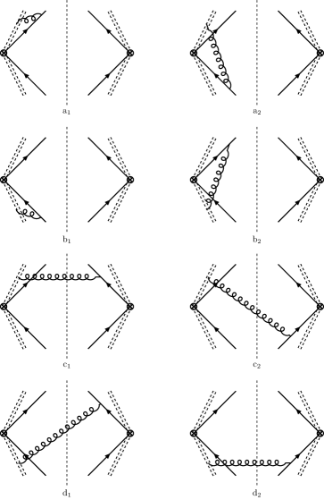
Figure 5: Diagrams showing the ultrasoft gluon exchanges between heavy-(anti)quarks and ultrasoft Wilson lines contributing to NLO. Hermitian conjugates are not shown. The dashed lines are illustrating the ultrasoft Wilson lines.

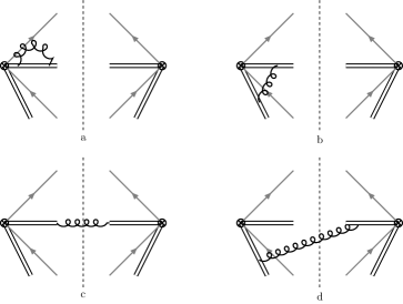
Figure 6: Non-zero diagrams showing the soft gluon exchange between soft Wilson lines contributing to NLO. Hermitian conjugates of diagrams a, b and d are not shown. The double lines are illustrating the soft Wilson lines.

The ultrasoft gluon exchanges between heavy (anti)quarks and ultrasoft Wilson lines, as illustrated in figure 5, originate from a single iteration of the chromo-electric term in the vNRQCD interaction Lagrangian (128) and the insertion of an ultrasoft gluon from the ultrasoft Wilson lines. As indicated in eq. (128), this contribution is directly proportional to the three-momentum of the heavy (anti)quark. Given the relationship $\bar{\mathbf{p}}=-\mathbf{p}$ between the 3-momenta of the heavy quark and antiquark, the sum $a1+a2$ evaluates to zero. This relationship holds true for the other pairs of diagrams as well: $b1+b2=0$, and so forth.

The soft gluon exchanges between soft Wilson lines are shown in the figure 6. To obtain the contribution of that kind of interactions we need compute the following integrals:

$$I^{\ref{fig:TMDShF-SoftExchange}\text{a}}(\mathbf{k}_{\perp}^{2};\mu) =ig^{2}C_{A}\mu^{2\varepsilon}\delta^{2}(\mathbf{k}_{\perp})\int\frac{d^{d}k}{(2\pi)^{d}}\frac{1}{(k^{2}+i0)}\frac{1}{(k^{0}+i0)(-k^{0}+i0)}+h.c.$$ (141)

$$=\frac{g^{2}C_{A}\mu^{2\varepsilon}}{2}\delta^{2}(\mathbf{k}_{\perp})\int\frac{d^{d-1}k}{(2\pi)^{d-1}}\frac{1}{|\mathbf{k}|^{3}}+h.c.$$

$$=\frac{\alpha_{s}C_{A}}{2\pi}\delta^{2}(\mathbf{k}_{\perp})\left(\frac{1}{\varepsilon_{\rm{UV}}}-\frac{1}{\varepsilon_{\rm{IR}}}\right)\;,$$

$$I^{\ref{fig:TMDShF-SoftExchange}\text{b}}(\mathbf{k}_{\perp}^{2};\mu) =-ig^{2}C_{A}\mu^{2\varepsilon}\delta^{2}(\mathbf{k}_{\perp})\int\frac{d^{d}k}{(2\pi)^{d}}\frac{1}{(k^{2}+i0)}\frac{v\cdot\bar{n}}{(k^{+}+i\delta^{+})(\frac{k^{+}v^{-}+k^{-}v^{+}}{2}+i0)}+h.c.$$

$$=\frac{-ig^{2}C_{A}\mu^{2\varepsilon}2(-2\pi i)}{2(2\pi)^{2}(2\pi)^{2-2\varepsilon}}\delta^{2}(\mathbf{k}_{\perp})\int_{0}^{\infty}\frac{dk^{+}d^{d-2}\mathbf{k}_{\perp}}{(k^{+}+i\delta^{+})(\mathbf{k}_{\perp}^{2}+k^{+2}(v^{-}/v^{+}))}+h.c.$$

$$=-\frac{g^{2}C_{A}}{2\pi}\frac{\Gamma(\varepsilon)\mu^{2\varepsilon}}{(4\pi)^{1-\varepsilon}(v^{-}/v^{+})^{\varepsilon}}\int_{0}^{\infty}\frac{dk^{+}(k^{+})^{-2\varepsilon}}{k^{+}+i\delta^{+}}+h.c.$$

$$=-2\alpha_{s}C_{A}\frac{(i\delta^{+})^{-2\varepsilon}}{(4\pi)^{1-\varepsilon}(v^{-}/v^{+})^{\varepsilon}}\Gamma(\varepsilon)\Gamma(2\varepsilon)\Gamma(1-2\varepsilon)+h.c.$$

$$=-\frac{\alpha_{s}C_{A}}{2\pi}\delta^{2}(\mathbf{k}_{\perp})\left[\frac{1}{\varepsilon_{\rm{UV}}^{2}}-\frac{1}{\varepsilon_{\rm{UV}}}\hbox{ln}\frac{\delta^{+2}(v^{-}/v^{+})}{\mu^{2}}+\frac{1}{2}\hbox{ln}^{2}\frac{\delta^{+2}(v^{-}/v^{+})}{\mu^{2}}+\frac{\pi^{2}}{4}\right]\;,$$

$$I^{\ref{fig:TMDShF-SoftExchange}\text{c}}(\mathbf{k}_{\perp}^{2};\mu) =2\pi g^{2}C_{A}\int\frac{d^{d}k}{(2\pi)^{d}}\frac{v^{2}\delta(k^{2})\theta(k^{+})}{(\frac{k^{+}+k^{-}}{2})(\frac{-k^{+}-k^{-}}{2})}$$ (142)

$$=-\alpha_{s}C_{A}2^{2\epsilon}\pi^{2\epsilon-2}\int_{0}^{\infty}\frac{dk^{+}d^{d-2}\mathbf{k}_{\perp}\left|k^{+}\right|}{\left(\mathbf{k}_{\perp}^{2}+(k^{+})^{2}\right)^{2}}$$

$$=-\frac{\alpha_{s}C_{A}}{2\pi^{2}}\frac{1}{\mathbf{k}_{\perp}^{2}}\;,$$

$$I^{\ref{fig:TMDShF-SoftExchange}\text{d}}(\mathbf{k}_{\perp}^{2};\mu) =-2\pi g^{2}C_{A}\int\frac{d^{d}k}{(2\pi)^{d}}\frac{v\cdot\bar{n}\,\delta(k^{2})\theta(k^{+})}{(k^{+}+i\delta^{+})(\frac{-k^{+}v^{-}-k^{-}v^{+}}{2})}+h.c.$$

$$=\frac{4\pi g^{2}C_{A}}{2(2\pi)^{2}(2\pi)^{2-2\varepsilon}}\int_{0}^{\infty}\frac{dk^{+}\,d^{d-2}\mathbf{k}_{\perp}}{(k^{+}+i\delta^{+})(\mathbf{k}_{\perp}^{2}+k^{+2}(v^{-}/v^{+}))}+h.c.$$

$$=-\frac{\alpha_{s}C_{A}}{2\pi^{2}}\frac{1}{\mathbf{k}_{\perp}^{2}-\delta^{+2}(v^{-}/v^{+})}\hbox{ln}\left(\frac{\delta^{+2}(v^{-}/v^{+})}{\mathbf{k}_{\perp}^{2}}\right)\;.$$

Here we only explicitly show the dependence on $v^{+}$ and $v^{-}$ in integrals b and d because as we will see later, it will be crucial for the renormalization of rapidity divergences. For the diagrams a and c, we use that $v$ is a time-like vector such that $v^{2}=1$ and $v^{-}/v^{+}=1$. Using the previous results, the contribution to the shape function of each diagram in figure 6, denoted by $i$, is the following:

$$S_{{}^{1}S_{0}^{[8]}}^{\ref{fig:TMDShF-SoftExchange}i}(\mathbf{k}_{\perp}^{2})=\left<{}^{1}S_{0}^{[8]}\right>^{\text{LO}}I^{\ref{fig:TMDShF-SoftExchange}i}(\mathbf{k}_{\perp}^{2}),\quad i=\text{a,b,c,d}\;.$$ (143)

Putting everything together, we get the total contribution of the soft gluon exchanges between soft Wilson lines:

$$S_{{}^{1}S_{0}^{[8]}}^{\ref{fig:TMDShF-SoftExchange}}(\mathbf{k}_{\perp}^{2};\mu,\delta) =-\left<{}^{1}S_{0}^{[8]}\right>^{\text{LO}}\frac{\alpha_{s}C_{A}}{2\pi^{2}}$$ (144)

$$\times \left[\pi\delta^{2}(\mathbf{k}_{\perp})\left(\frac{1}{\varepsilon_{\rm{UV}}^{2}}-\frac{1}{\varepsilon_{\rm{UV}}}\hbox{ln}\frac{\delta^{2}}{\mu^{2}}+\frac{1}{2}\hbox{ln}^{2}\frac{\delta^{2}}{\mu^{2}}+\frac{\pi^{2}}{4}\right)+\frac{1}{\mathbf{k}_{\perp}^{2}-\delta^{2}}\hbox{ln}\left(\frac{\delta^{2}}{\mathbf{k}_{\perp}^{2}}\right)\right.$$

$$\left.+\delta^{2}(\mathbf{k}_{\perp})\left(\frac{\pi}{\varepsilon_{\rm{IR}}}-\frac{\pi}{\varepsilon_{\rm{UV}}}\right)+\frac{1}{\mathbf{k}_{\perp}^{2}}\right]\;.$$

Here we define $\delta^{2}\equiv\delta^{+2}(v^{-}/v^{+})$ which is boost invariant. Since there is only one soft Wilson line having rapidity divergences, only diagrams exhibiting rapidity divergences are b and d and the sum of their contributions is half of soft function.

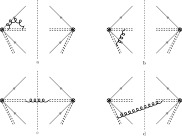
Figure 7: Non-zero diagrams showing the ultrasoft gluon exchange between ultrasoft Wilson lines contributing to NLO. Hermitian conjugates of diagrams a, b and d are not shown. The dashed lines are illustrating the ultrasoft Wilson lines.

The exchanges of usoft gluons between the ultrasoft Wilson lines are depicted in figure 7. These diagrams yield scaleless integrals. For instance, the integral arising from the virtual interaction between the ultrasoft Wilson lines $n$ and $v$, after integrating over $k^{0}$, is as follows:

$$I^{us}=\int\frac{d^{4}k}{(2\pi)^{4}}\frac{g^{2}\,v\cdot\bar{n}}{(k^{0})^{2}[(k^{0})^{2}-\mathbf{k}^{2}+i\varepsilon]}=ig^{2}\int\frac{d^{3}k}{(2\pi)^{3}}\frac{v\cdot\bar{n}}{|\mathbf{k}|^{3}}\;.$$ (145)

According to distinguish between IR and UV poles, we would have to take into account the contribution of these diagrams to the TMDShF. However it will cancel against the zero-bin subtraction of the corresponding soft diagrams shown in figure 6.

Summing all the results obtained in this section, we get the TMD shape function at NLO in transverse momentum space:

$$S_{{}^{1}S_{0}^{[8]}}(\mathbf{k}_{\perp};\mu,\delta) =\frac{\alpha_{s}}{2\pi}\delta^{2}(\mathbf{k}_{\perp})\left((C_{F}-C_{A}/2)\frac{\pi^{2}}{\text{v}}-\frac{C_{A}}{\varepsilon_{\rm{IR}}}\right)\left<{}^{1}S_{0}^{[8]}\right>^{\text{LO}}$$ (146)

$$-\frac{\alpha_{s}C_{A}}{2\pi^{2}}\pi\delta^{2}(\mathbf{k}_{\perp})\left(\frac{1}{\varepsilon_{\rm{UV}}^{2}}-\frac{1}{\varepsilon_{\rm{UV}}}\hbox{ln}\frac{\delta^{2}}{\mu^{2}}+\frac{1}{2}\hbox{ln}^{2}\frac{\delta^{2}}{\mu^{2}}+\frac{\pi^{2}}{4}\right)\left<{}^{1}S_{0}^{[8]}\right>^{\text{LO}}$$

$$-\frac{\alpha_{s}C_{A}}{2\pi^{2}}\frac{1}{\mathbf{k}_{\perp}^{2}-\delta^{2}}\hbox{ln}\left(\frac{\delta^{2}}{\mathbf{k}_{\perp}^{2}}\right)\left<{}^{1}S_{0}^{[8]}\right>^{\text{LO}}$$

$$+\frac{\alpha_{s}C_{A}}{2\pi^{2}}\left(\frac{\pi}{\varepsilon_{\rm{UV}}}\delta^{2}(\mathbf{k}_{\perp})-\frac{1}{\mathbf{k}_{\perp}^{2}}\right)\left<{}^{1}S_{0}^{[8]}\right>^{\text{LO}}$$

$$+\frac{4\alpha_{s}}{3\pi^{2}m_{c}^{2}}\frac{1}{\mathbf{k}_{\perp}^{2}}\left(C_{F}\left<{}^{1}P_{1}^{[1]}\right>^{\text{LO}}+B_{F}\left<{}^{1}P_{1}^{[8]}\right>^{\text{LO}}\right)\;.$$

Before anything else, it is convenient to perform the Fourier transform of the shape function such that:

$$S_{{}^{1}S_{0}^{[8]}}(b_{T};\mu,\delta) =\left<{}^{1}S_{0}^{[8]}\right>^{\text{LO}}\left[\frac{\alpha_{s}C_{A}}{2\pi}\left(\frac{1}{\varepsilon_{\rm{UV}}}+L_{T}\right)+\frac{\pi\alpha_{s}}{2\text{v}}\left(C_{F}-C_{A}/2\right)\right.$$ (147)

$$\left.+\frac{\alpha_{s}C_{A}}{2\pi}\left(-\frac{1}{\varepsilon_{\rm{UV}}^{2}}+\frac{1}{\varepsilon_{\rm{UV}}}\hbox{ln}\frac{\delta^{2}}{\mu^{2}}+\frac{L_{T}^{2}}{2}+L_{T}\hbox{ln}\frac{\delta^{2}}{\mu^{2}}+\frac{\pi^{2}}{12}\right)\right]$$

$$-\frac{4\alpha_{s}}{3\pi m_{c}^{2}}\left(\frac{1}{\varepsilon_{\rm{IR}}}+L_{T}\right)\left(C_{F}\left<{}^{1}P_{1}^{[1]}\right>^{\text{LO}}+B_{F}\left<{}^{1}P_{1}^{[8]}\right>^{\text{LO}}\right)\;,$$

with $L_{T}=\hbox{ln}(\mu^{2}b_{T}^{2}e^{2\gamma_{E}}/4)$. Note we employ the same symbols to denote functions in $k_{T}$-space and in $b_{T}$-space. To perform the Fourier transform, we need the following integrals:

$$\int d^{2-2\varepsilon}\mathbf{k}_{\perp}\frac{e^{i\mathbf{k}_{\perp}\cdot\mathbf{b}_{\perp}}}{\mathbf{k}_{\perp}^{2}} =4^{-\varepsilon}\pi^{1-\varepsilon}b_{T}^{2\varepsilon}\Gamma(-\varepsilon)\;,$$ (148)

$$\int d^{2-2\varepsilon}\mathbf{k}_{\perp}\frac{e^{i\mathbf{k}_{\perp}\cdot\mathbf{b}_{\perp}}}{k_{T}^{2}-\Lambda^{2}}\,\hbox{ln}\frac{\Lambda^{2}}{k_{T}^{2}} =-\pi\left(\frac{1}{2}\hbox{ln}^{2}\frac{4e^{-2\gamma_{E}}}{\Lambda^{2}b_{T}^{2}}+\frac{\pi^{2}}{3}\right)\;.$$

We proceed to renormalize the rapidity divergences by redefining the shape function as in eq. (38). The soft function was calculated, e.g., in Echevarria:2015uaa , its Fourier-transformed result at NLO is

$$S(b_{T};\mu,\delta^{+},\delta^{-})=\frac{\alpha_{s}C_{A}}{2\pi}\left[-\frac{2}{\varepsilon_{\rm{UV}}^{2}}+\frac{2}{\varepsilon_{\rm{UV}}}\hbox{ln}\frac{\delta^{+}\delta^{-}}{\mu^{2}}+L_{T}^{2}+2L_{T}\hbox{ln}\frac{\delta^{+}\delta^{-}}{\mu^{2}}+\frac{\pi^{2}}{6}\right]\;.$$ (149)

According to the discussions in Echevarria:2012js , the soft function splits (to all orders) into two pieces:

$$S(b_{T};\mu,\delta^{+},\delta^{-})=\sqrt{S(b_{T};\mu,\delta^{+},\tfrac{\delta+}{\alpha})}\,\sqrt{S(b_{T};\mu,\alpha\delta^{-},\delta^{-})}\;,$$ (150)

where then at NLO we have

$$S(b_{T};\mu,\delta^{+},\tfrac{\delta^{+}}{\alpha})=\frac{\alpha_{s}C_{A}}{2\pi}\left[-\frac{2}{\varepsilon_{\rm{UV}}^{2}}+\frac{2}{\varepsilon_{\rm{UV}}}\hbox{ln}\frac{\delta^{+2}}{\alpha\mu^{2}}+L_{T}^{2}+2L_{T}\hbox{ln}\frac{\delta^{+2}}{\alpha\mu^{2}}+\frac{\pi^{2}}{6}\right]\;,$$ (151)

where $\alpha$ is a real number which transforms under boosts like $(p^{+})^{2}$. Here we define this number such that $\alpha/(v^{-}/v^{+})\equiv\zeta_{B}$, where the factor $\zeta_{B}$ is a finite boost dimensionless invariant real number. The procedure to get $\zeta_{B}$ is the TMD factorization theorem, similar to the one used, e.g., in Echevarria:2012js : in that case, $\zeta_{A}$ and $\zeta_{B}$ have dimensions, but in the case that concerns us, $\zeta_{B}$ is dimensionless and $\zeta_{A}$ has mass-squared dimensions. Consequently, we have $\zeta_{A}\zeta_{B}=Q_{H}^{2}$ in this work. Note the similarity to the process of dijet production in DIS delCastillo:2020omr . Given that the shape function in the previous result includes a contribution from half of the soft function (look at second line in eq. (147)), the renormalization using the Fourier-transformed soft function in eq. (151) is straightforward. Consequently, the rapidity renormalization scale $\zeta_{B}$ emerges, and the subtracted ${}^{1}S_{0}^{[8]}$ TMDShF at NLO is as follows:

$$S_{{}^{1}S_{0}^{[8]}}(b_{T};\mu,\zeta_{B})=\left<{}^{1}S_{0}^{[8]}\right>^{\text{LO}}+\frac{\alpha_{s}}{2\pi}\Bigg{[}\frac{C_{A}}{\varepsilon_{\rm{UV}}}\left(1-\hbox{ln}\,\zeta_{B}\right)\left<{}^{1}S_{0}^{[8]}\right>^{\text{LO}}$$ (152)

$$\quad+C_{A}L_{T}\left(1-\hbox{ln}\,\zeta_{B}\right)\left<{}^{1}S_{0}^{[8]}\right>^{\text{LO}}-\frac{8}{3m_{c}^{2}}L_{T}\left(C_{F}\left<{}^{1}P_{1}^{[1]}\right>^{\text{LO}}+B_{F}\left<{}^{1}P_{1}^{[8]}\right>^{\text{LO}}\right)$$

$$\quad+\frac{\pi^{2}}{\text{v}}(C_{F}-C_{A}/2)\left<{}^{1}S_{0}^{[8]}\right>^{\text{LO}}-\frac{8}{3m_{c}^{2}}\frac{1}{\varepsilon_{\rm{IR}}}\left(C_{F}\left<{}^{1}P_{1}^{[1]}\right>^{\text{LO}}+B_{F}\left<{}^{1}P_{1}^{[8]}\right>^{\text{LO}}\right)\Bigg{]}\;.$$

At NLO, we have explicitly verified, through the utilization of the $\delta$-regularization scheme, the expected cancellation of rapidity divergences. It’s noteworthy to observe an additional UV divergence in eq. (LABEL:eq:ShTotal) compared to the LDME calculation in eq. (137). This divergence, stemming from the virtual gluon self-exchanges of the $\bar{c}c$ state depicted in figure 6a, is relevant in the RG evolution of the shape functions, as we see in section 3.

Appendix D Results for P-states

As previously mentioned, the computation of the ${}^{3}P_{J}^{[8]}$ LDMEs and TMDShFs can be inferred from the S-wave calculation. In this section, we summarize the results for the P-wave channel.

Upon inspection of the diagrams and the vNRQCD Lagrangian interaction, it becomes evident that the methodology for computing the P-waves mirrors that of the S-wave. At LO, the LDME primarily encompasses the spin factor denoting the configuration of angular momentum, spin, and color of the heavy quarks in the final state. Analogous to our explanation in eq. (120) and in eq. (121), and taking the operators in NRQCD, the LDMEs are as follows

$$\left<{}^{3}P_{0}^{[8]}\right>^{\text{LO}} =\frac{M^{2}}{3}\,\eta^{\dagger}\mathbf{q}\cdot\boldsymbol{\sigma}T^{a}\xi\times\xi^{\dagger}\mathbf{q}\cdot\boldsymbol{\sigma}T^{a}\xi\eta\;,$$ (153)

$$\left<{}^{3}P_{1}^{[8]}\right>^{\text{LO}} =\frac{M^{2}}{2}\,\eta^{\dagger}(\mathbf{q}\times\boldsymbol{\sigma})^{k}T^{a}\xi\times\xi^{\dagger}(\mathbf{q}\times\boldsymbol{\sigma})^{k}T^{a}\xi\eta\;,$$

$$\left<{}^{3}P_{2}^{[8]}\right>^{\text{LO}} =M^{2}\,\eta^{\dagger}q^{(i}\sigma^{j)}T^{a}\xi\times\xi^{\dagger}q^{(i}\sigma^{j)}T^{a}\xi\eta\;.$$

Here we do not write the boost matrix (94) because we are considering this result in the $J/\psi$ rest frame. Consequently, the exchange of soft and ultrasoft gluons originating from the vNRQCD interaction Lagrangian yields analogous contributions for the P-wave as observed for the S-wave. The chromo-electric term corresponds to a label operator which gives a three-momentum in the spin factor. This, in turn, corresponds to an angular momentum with a value one unit higher than that of the LO spin factor. For instance, if the LO spin factor has angular momentum $L$, the chromo-electric term provides a combination of the color singlet and color octet for an angular momentum value of $L+1$:

$$\left<{}^{2S+1}L_{J}^{[8]}\right>^{\ref{fig:TMDShF-ChroElectric}}=\frac{4\alpha_{s}}{3\pi m_{c}^{2}}\left(C_{F}\left<{}^{2S+1}{L^{\prime}}_{J^{\prime}}^{[1]}\right>^{\text{LO}}+B_{F}\left<{}^{2S+1}{L^{\prime}}_{J^{\prime}}^{[8]}\right>^{\text{LO}}\right)\left(\frac{1}{\varepsilon_{\rm{UV}}}-\frac{1}{\varepsilon_{\rm{IR}}}\right)\;,$$ (154)

with $L^{\prime}=L+1$, and therefore $J^{\prime}=J+1$ (the spin $S$ remains unchanged). From this result and considering that the Coulomb singularity always appears regardless of the state, we have that the LDME at NLO is

$$\left<{}^{3}P_{J}^{[8]}\right>^{\text{NLO}} =\left(1+\left(C_{F}-C_{A}/2\right)\frac{\pi\alpha_{s}}{2\text{v}}\right)\left<{}^{3}P_{J}^{[8]}\right>^{\text{LO}}$$ (155)

$$+\frac{4\alpha_{s}}{3\pi m_{c}^{2}}\left(C_{F}\left<{}^{3}D_{J+1}^{[1]}\right>^{\text{LO}}+B_{F}\left<{}^{3}D_{J+1}^{[8]}\right>^{\text{LO}}\right)\left(\frac{1}{\varepsilon_{\rm{UV}}}-\frac{1}{\varepsilon_{\rm{IR}}}\right)\;.$$

Regarding the shape function, gluon exchanges between the Wilson lines do not affect the state of the heavy quark pair, so the integrals in eqs. (141) and (142) remain unchanged. Consequently, the result in eq. (147) also remains the same, and therefore at the end of the day, we find that the shape function at NLO is:

$$S_{{}^{3}P_{J}^{[8]}\to J/\psi}(b_{T};\mu,\zeta_{B})=\frac{1}{N^{(J)}_{pol}}\left\{\left<{}^{3}P_{J}^{[8]}\right>^{\text{LO}}+\frac{\alpha_{s}}{2\pi}\Bigg{[}\frac{C_{A}}{\varepsilon_{\rm{UV}}}\left(1-\hbox{ln}\,\zeta_{B}\right)\left<{}^{3}P_{J}^{[8]}\right>^{\text{LO}}\right.$$ (156)

$$\left.\quad+C_{A}L_{T}\left(1-\hbox{ln}\,\zeta_{B}\right)\left<{}^{3}P_{J}^{[8]}\right>^{\text{LO}}-\frac{8}{3m_{c}^{2}}L_{T}\left(C_{F}\left<{}^{3}D_{J+1}^{[1]}\right>^{\text{LO}}+B_{F}\left<{}^{3}D_{J+1}^{[8]}\right>^{\text{LO}}\right)\right.$$

$$\left.\quad+\frac{\pi^{2}}{\text{v}}(C_{F}-C_{A}/2)\left<{}^{3}P_{J}^{[8]}\right>^{\text{LO}}-\frac{8}{3m_{c}^{2}}\frac{1}{\varepsilon_{\rm{IR}}}\left(C_{F}\left<{}^{3}D_{J+1}^{[1]}\right>^{\text{LO}}+B_{F}\left<{}^{3}D_{J+1}^{[8]}\right>^{\text{LO}}\right)\Bigg{]}\right\}\;.$$

References

- (1) R. Abdul Khalek et al., “Science Requirements and Detector Concepts for the Electron-Ion Collider: EIC Yellow Report,” Nucl. Phys. A 1026 (2022) 122447, arXiv:2103.05419 [physics.ins-det].
- (2) S. Fleming and T. Mehen, “Leptoproduction of J / psi,” Phys. Rev. D 57 (1998) 1846–1857, arXiv:hep-ph/9707365.
- (3) B. A. Kniehl and L. Zwirner, “ inclusive production in deep inelastic scattering at DESY HERA,” Nucl. Phys. B 621 (2002) 337–358, arXiv:hep-ph/0112199.
- (4) R. M. Godbole, A. Misra, A. Mukherjee, and V. S. Rawoot, “Transverse Single Spin Asymmetry in and Transverse Momentum Dependent Evolution of the Sivers Function,” Phys. Rev. D88 no. 1, (2013) 014029, arXiv:1304.2584 [hep-ph].
- (5) A. Mukherjee and S. Rajesh, “ production in polarized and unpolarized ep collision and Sivers and asymmetries,” Eur. Phys. J. C77 no. 12, (2017) 854, arXiv:1609.05596 [hep-ph].
- (6) S. Rajesh, R. Kishore, and A. Mukherjee, “Sivers effect in Inelastic Photoproduction in Collision in Color Octet Model,” Phys. Rev. D98 no. 1, (2018) 014007, arXiv:1802.10359 [hep-ph].
- (7) A. Bacchetta, D. Boer, C. Pisano, and P. Taels, “Gluon TMDs and NRQCD matrix elements in production at an EIC,” Eur. Phys. J. C 80 no. 1, (2020) 72, arXiv:1809.02056 [hep-ph].
- (8) U. D’Alesio, F. Murgia, C. Pisano, and P. Taels, “Azimuthal asymmetries in semi-inclusive production at an EIC,” Phys. Rev. D 100 no. 9, (2019) 094016, arXiv:1908.00446 [hep-ph].
- (9) D. Boer, U. D’Alesio, F. Murgia, C. Pisano, and P. Taels, “J/ meson production in SIDIS: matching high and low transverse momentum,” JHEP 09 (2020) 040, arXiv:2004.06740 [hep-ph].
- (10) U. D’Alesio, L. Maxia, F. Murgia, C. Pisano, and S. Rajesh, “J/ polarization in semi-inclusive DIS at low and high transverse momentum,” JHEP 03 (2022) 037, arXiv:2110.07529 [hep-ph].
- (11) A. Colpani Serri, Y. Feng, C. Flore, J.-P. Lansberg, M. A. Ozcelik, H.-S. Shao, and Y. Yedelkina, “Revisiting nlo qcd corrections to total inclusive and photoproduction cross sections in lepton-proton collisions,” Phys. Lett. B 835 (2022) 137556, arXiv:2112.05060 [hep-ph].
- (12) R. Kishore, A. Mukherjee, A. Pawar, and M. Siddiqah, “cos2t azimuthal asymmetry in back-to-back J/-jet production in ep→eJ/ jet X at the EIC,” Phys. Rev. D 106 no. 3, (2022) 034009, arXiv:2203.13516 [hep-ph].
- (13) J. Bor and D. Boer, “TMD evolution study of the azimuthal asymmetry in unpolarized production at EIC,” Phys. Rev. D 106 no. 1, (2022) 014030, arXiv:2204.01527 [hep-ph].
- (14) U. D’Alesio, L. Maxia, F. Murgia, C. Pisano, and S. Rajesh, “J/ polarization in large-PT semi-inclusive deep-inelastic scattering at the EIC,” Phys. Rev. D 107 no. 11, (2023) 114001, arXiv:2301.11987 [hep-ph].
- (15) D. Boer, J. Bor, L. Maxia, C. Pisano, and F. Yuan, “Transverse momentum dependent shape function for J/ production in SIDIS,” JHEP 08 (2023) 105, arXiv:2304.09473 [hep-ph].
- (16) Z.-B. Kang, E. Li, and F. Salazar, “Direct quarkonium-plus-gluon production in DIS in the color glass condensate,” JHEP 03 (2024) 027, arXiv:2310.12102 [hep-ph].
- (17) L. Maxia and F. Yuan, “Azimuthal Angular Correlation of Plus Jet Production at the EIC,” arXiv:2403.02097 [hep-ph].
- (18) N. Kato, L. Maxia, and C. Pisano, “Spin asymmetries for -even quarkonium production as a probe of gluon distributions,” arXiv:2403.20017 [hep-ph].
- (19) W. J. den Dunnen, J. P. Lansberg, C. Pisano, and M. Schlegel, “Accessing the Transverse Dynamics and Polarization of Gluons inside the Proton at the LHC,” Phys. Rev. Lett. 112 (2014) 212001, arXiv:1401.7611 [hep-ph].
- (20) J.-P. Lansberg, C. Pisano, and M. Schlegel, “Associated production of a dilepton and a at the LHC as a probe of gluon transverse momentum dependent distributions,” Nucl. Phys. B920 (2017) 192–210, arXiv:1702.00305 [hep-ph].
- (21) J.-P. Lansberg, C. Pisano, F. Scarpa, and M. Schlegel, “Pinning down the linearly-polarised gluons inside unpolarised protons using quarkonium-pair production at the LHC,” Phys. Lett. B784 (2018) 217–222, arXiv:1710.01684 [hep-ph]. [Erratum: Phys. Lett.B791,420(2019)].
- (22) F. Scarpa, Probing the gluon Transverse Momentum-Dependent distributions inside the proton through quarkonium-pair production at the LHC. PhD thesis, High-Energy Frontier, Groningen U., Groningen U., U. Paris-Saclay, 2020.
- (23) F. Scarpa, D. Boer, M. G. Echevarria, J.-P. Lansberg, C. Pisano, and M. Schlegel, “Studies of gluon TMDs and their evolution using quarkonium-pair production at the LHC,” Eur. Phys. J. C 80 no. 2, (2020) 87, arXiv:1909.05769 [hep-ph].
- (24) ALICE, ATLAS, CMS, LHCb Collaboration, Y. Wei, “Associated production of quarkonium pairs at LHC,” PoS LHCP2023 (2024) 033.
- (25) Q.-L. Jia, A.-P. Chen, and Y.-G. Xu, “Single parton fragmentation functions of heavy quarkonium in soft gluon factorization,” Phys. Rev. D 109 no. 3, (2024) 034039, arXiv:2402.04709 [hep-ph].
- (26) K. Lee and G. Sterman, “Power expansion for heavy quarkonium production at next-to-leading order in annihilation,” JHEP 09 (2020) 046, arXiv:2006.07375 [hep-ph].
- (27) Belle-II Collaboration, R. Garg, “Recent quarkonium results from Belle II,” PoS HQL2023 (2024) 038.
- (28) G.-Y. Wang, X.-C. Zheng, X.-G. Wu, and G.-Z. Xu, “Z-boson decays into S-wave quarkonium plus a photon up to O(sv2) corrections,” Phys. Rev. D 109 no. 7, (2024) 074004, arXiv:2312.08796 [hep-ph].
- (29) G. T. Bodwin, H. S. Chung, J.-H. Ee, and J. Lee, “-boson decays to a vector quarkonium plus a photon,” Phys. Rev. D 97 no. 1, (2018) 016009, arXiv:1709.09320 [hep-ph].
- (30) A. P. Martynenko and F. A. Martynenko, “Relativistic Corrections to the Higgs Boson Decay into a Pair of Vector Quarkonia,” Symmetry 15 no. 2, (2023) 448.
- (31) H. Dong, P. Sun, and B. Yan, “Probing the H coupling via Higgs boson exclusive decay into quarkonia plus a photon at the HL-LHC,” Phys. Rev. D 106 no. 9, (2022) 095013, arXiv:2208.05153 [hep-ph].
- (32) E. Chapon et al., “Prospects for quarkonium studies at the high-luminosity LHC,” Prog. Part. Nucl. Phys. 122 (2022) 103906, arXiv:2012.14161 [hep-ph].
- (33) J.-P. Lansberg, “New Observables in Inclusive Production of Quarkonia,” Phys. Rept. 889 (2020) 1–106, arXiv:1903.09185 [hep-ph].
- (34) M. G. Echevarria, Y. Makris, and I. Scimemi, “Quarkonium TMD fragmentation functions in NRQCD,” JHEP 10 (2020) 164, arXiv:2007.05547 [hep-ph].
- (35) F. G. Celiberto, “Vector Quarkonia at the LHC with Jethad: A High-Energy Viewpoint,” Universe 9 no. 7, (2023) 324, arXiv:2305.14295 [hep-ph].
- (36) L. Dai, C. Kim, and A. K. Leibovich, “Heavy quark transverse momentum dependent fragmentation,” arXiv:2310.19207 [hep-ph].
- (37) M. Copeland, S. Fleming, R. Gupta, R. Hodges, and T. Mehen, “Polarized J/ production in semi-inclusive DIS at large Q2: Comparing quark fragmentation and photon-gluon fusion,” Phys. Rev. D 109 no. 7, (2024) 074032, arXiv:2310.13737 [hep-ph].
- (38) M. G. Echevarria, S. F. Romera, and I. Scimemi, “Gluon TMD fragmentation function into quarkonium,” arXiv:2308.12356 [hep-ph].
- (39) M. Copeland, S. Fleming, R. Gupta, R. Hodges, and T. Mehen, “Polarized TMD fragmentation functions for J/ production,” Phys. Rev. D 109 no. 5, (2024) 054017, arXiv:2308.08605 [hep-ph].
- (40) R. von Kuk, J. K. L. Michel, and Z. Sun, “Transverse Momentum-Dependent Heavy-Quark Fragmentation at Next-to-Leading Order,” arXiv:2404.08622 [hep-ph].
- (41) M. Beneke, I. Z. Rothstein, and M. B. Wise, “Kinematic enhancement of nonperturbative corrections to quarkonium production,” Phys. Lett. B 408 (1997) 373–380, arXiv:hep-ph/9705286.
- (42) M. Neubert, “QCD based interpretation of the lepton spectrum in inclusive anti-B — X(u) lepton anti-neutrino decays,” Phys. Rev. D 49 (1994) 3392–3398, arXiv:hep-ph/9311325.
- (43) S. Fleming, A. K. Leibovich, and T. Mehen, “Resummation of Large Endpoint Corrections to Color-Octet Photoproduction,” Phys. Rev. D 74 (2006) 114004, arXiv:hep-ph/0607121.
- (44) S. Fleming, A. K. Leibovich, and T. Mehen, “Resumming the color octet contribution to + ,” Phys. Rev. D 68 (2003) 094011, arXiv:hep-ph/0306139.
- (45) M. G. Echevarria, “Proper TMD factorization for quarkonia production: as a study case,” arXiv:1907.06494 [hep-ph].
- (46) S. Fleming, Y. Makris, and T. Mehen, “An effective field theory approach to quarkonium at small transverse momentum,” JHEP 04 (2020) 122, arXiv:1910.03586 [hep-ph].
- (47) P. J. Mulders and J. Rodrigues, “Transverse momentum dependence in gluon distribution and fragmentation functions,” Phys. Rev. D 63 (2001) 094021, arXiv:hep-ph/0009343.
- (48) S. Meissner, A. Metz, and K. Goeke, “Relations between generalized and transverse momentum dependent parton distributions,” Phys. Rev. D 76 (2007) 034002, arXiv:hep-ph/0703176.
- (49) M. G. Echevarria, T. Kasemets, P. J. Mulders, and C. Pisano, “QCD evolution of (un)polarized gluon TMDPDFs and the Higgs -distribution,” JHEP 07 (2015) 158, arXiv:1502.05354 [hep-ph]. [Erratum: JHEP 05, 073 (2017)].
- (50) G. T. Bodwin, E. Braaten, and G. P. Lepage, “Rigorous QCD analysis of inclusive annihilation and production of heavy quarkonium,” Phys. Rev. D51 (1995) 1125–1171, arXiv:hep-ph/9407339 [hep-ph]. [Erratum: Phys. Rev.D55,5853(1997)].
- (51) G. C. Nayak, J.-W. Qiu, and G. F. Sterman, “Fragmentation, NRQCD and NNLO factorization analysis in heavy quarkonium production,” Phys. Rev. D 72 (2005) 114012, arXiv:hep-ph/0509021.
- (52) G. C. Nayak, J.-W. Qiu, and G. F. Sterman, “Fragmentation, factorization and infrared poles in heavy quarkonium production,” Phys. Lett. B 613 (2005) 45–51, arXiv:hep-ph/0501235.
- (53) Z.-B. Kang, J.-W. Qiu, and G. Sterman, “Factorization and quarkonium production,” Nucl. Phys. B Proc. Suppl. 214 (2011) 39–43.
- (54) Z.-B. Kang, Y.-Q. Ma, J.-W. Qiu, and G. Sterman, “Heavy Quarkonium Production at Collider Energies: Factorization and Evolution,” Phys. Rev. D 90 no. 3, (2014) 034006, arXiv:1401.0923 [hep-ph].
- (55) M. Butenschoen and B. A. Kniehl, “World data of J/psi production consolidate NRQCD factorization at NLO,” Phys. Rev. D 84 (2011) 051501, arXiv:1105.0820 [hep-ph].
- (56) H. S. Shao, H. Han, Y. Q. Ma, C. Meng, Y. J. Zhang, and K. T. Chao, “Yields and polarizations of prompt and production in hadronic collisions,” JHEP 05 (2015) 103, arXiv:1411.3300 [hep-ph].
- (57) G. T. Bodwin, K.-T. Chao, H. S. Chung, U.-R. Kim, J. Lee, and Y.-Q. Ma, “Fragmentation contributions to hadroproduction of prompt, , and states,” Phys. Rev. D 93 no. 3, (2016) 034041, arXiv:1509.07904 [hep-ph].
- (58) Y. Feng, B. Gong, C.-H. Chang, and J.-X. Wang, “Remaining parts of the long-standing polarization puzzle,” Phys. Rev. D 99 no. 1, (2019) 014044, arXiv:1810.08989 [hep-ph].
- (59) N. Brambilla, H. S. Chung, A. Vairo, and X.-P. Wang, “Inclusive production of J/, (2S), and states in pNRQCD,” JHEP 03 (2023) 242, arXiv:2210.17345 [hep-ph].
- (60) E. Braaten, “Introduction to the NRQCD factorization approach to heavy quarkonium,” in 3rd International Workshop on Particle Physics Phenomenology. 11, 1996. arXiv:hep-ph/9702225.
- (61) G. A. Schuler, “Quarkonium production: Velocity scaling rules and long distance matrix elements,” Int. J. Mod. Phys. A 12 (1997) 3951–3964, arXiv:hep-ph/9702230.
- (62) I. Z. Rothstein, P. Shrivastava, and I. W. Stewart, “Manifestly Soft Gauge Invariant Formulation of vNRQCD,” Nucl. Phys. B 939 (2019) 405–428, arXiv:1806.07398 [hep-ph].
- (63) E. Braaten and T. C. Yuan, “Gluon fragmentation into P wave heavy quarkonium,” Phys. Rev. D 50 (1994) 3176–3180, arXiv:hep-ph/9403401.
- (64) E. Braaten and S. Fleming, “Color octet fragmentation and the psi-prime surplus at the Tevatron,” Phys. Rev. Lett. 74 (1995) 3327–3330, arXiv:hep-ph/9411365.
- (65) J. P. Ma, “Quark fragmentation into p wave triplet quarkonium,” Phys. Rev. D 53 (1996) 1185–1190, arXiv:hep-ph/9504263.
- (66) E. Braaten and Y.-Q. Chen, “Dimensional regularization in quarkonium calculations,” Phys. Rev. D 55 (1997) 2693–2707, arXiv:hep-ph/9610401.
- (67) A. Petrelli, M. Cacciari, M. Greco, F. Maltoni, and M. L. Mangano, “NLO production and decay of quarkonium,” Nucl. Phys. B514 (1998) 245–309, arXiv:hep-ph/9707223 [hep-ph].
- (68) C. W. Bauer, S. Fleming, and M. E. Luke, “Summing Sudakov logarithms in B —¿ X(s gamma) in effective field theory,” Phys. Rev. D63 (2000) 014006, arXiv:hep-ph/0005275 [hep-ph].
- (69) C. W. Bauer, D. Pirjol, and I. W. Stewart, “Soft collinear factorization in effective field theory,” Phys. Rev. D65 (2002) 054022, arXiv:hep-ph/0109045 [hep-ph].
- (70) C. W. Bauer and I. W. Stewart, “Invariant operators in collinear effective theory,” Phys. Lett. B516 (2001) 134–142, arXiv:hep-ph/0107001 [hep-ph].
- (71) M. Beneke, A. P. Chapovsky, M. Diehl, and T. Feldmann, “Soft collinear effective theory and heavy to light currents beyond leading power,” Nucl. Phys. B643 (2002) 431–476, arXiv:hep-ph/0206152 [hep-ph].
- (72) C. W. Bauer, D. Pirjol, and I. W. Stewart, “Factorization and endpoint singularities in heavy to light decays,” Phys. Rev. D 67 (2003) 071502, arXiv:hep-ph/0211069.
- (73) H. Georgi, “An Effective Field Theory for Heavy Quarks at Low-energies,” Phys. Lett. B 240 (1990) 447–450.
- (74) M. Boglione, A. Dotson, L. Gamberg, S. Gordon, J. O. Gonzalez-Hernandez, A. Prokudin, T. C. Rogers, and N. Sato, “Mapping the Kinematical Regimes of Semi-Inclusive Deep Inelastic Scattering,” JHEP 10 (2019) 122, arXiv:1904.12882 [hep-ph].
- (75) I. Scimemi and A. Vladimirov, “Non-perturbative structure of semi-inclusive deep-inelastic and Drell-Yan scattering at small transverse momentum,” JHEP 06 (2020) 137, arXiv:1912.06532 [hep-ph].
- (76) M. G. Echevarria, I. Scimemi, and A. Vladimirov, “Unpolarized Transverse Momentum Dependent Parton Distribution and Fragmentation Functions at next-to-next-to-leading order,” JHEP 09 (2016) 004, arXiv:1604.07869 [hep-ph].
- (77) A. V. Manohar and I. W. Stewart, “The Zero-Bin and Mode Factorization in Quantum Field Theory,” Phys. Rev. D 76 (2007) 074002, arXiv:hep-ph/0605001.
- (78) D. Boer, S. Cotogno, T. van Daal, P. J. Mulders, A. Signori, and Y.-J. Zhou, “Gluon and Wilson loop TMDs for hadrons of spin 1,” JHEP 10 (2016) 013, arXiv:1607.01654 [hep-ph].
- (79) Y.-Q. Ma, T. Stebel, and R. Venugopalan, “ polarization in the CGC+NRQCD approach,” JHEP 12 (2018) 057, arXiv:1809.03573 [hep-ph].
- (80) N. Brambilla, W. Chen, Y. Jia, V. Shtabovenko, and A. Vairo, “Relativistic corrections to exclusive production from annihilation,” Phys. Rev. D 97 no. 9, (2018) 096001, arXiv:1712.06165 [hep-ph]. [Erratum: Phys.Rev.D 101, 039903 (2020)].
- (81) J. A. R. Coope and R. F. Snider, “Irreducible Cartesian Tensors. II. General Formulation,” Journal of Mathematical Physics 11 no. 3, (03, 1970) 1003–1017. https://doi.org/10.1063/1.1665190.
- (82) F. Maltoni, M. L. Mangano, and A. Petrelli, “Quarkonium photoproduction at next-to-leading order,” Nucl. Phys. B 519 (1998) 361–393, arXiv:hep-ph/9708349.
- (83) M. G. Echevarria, A. Idilbi, A. Schäfer, and I. Scimemi, “Model-Independent Evolution of Transverse Momentum Dependent Distribution Functions (TMDs) at NNLL,” Eur. Phys. J. C73 no. 12, (2013) 2636, arXiv:1208.1281 [hep-ph].
- (84) M. G. Echevarria, I. Scimemi, and A. Vladimirov, “Universal transverse momentum dependent soft function at NNLO,” Phys. Rev. D93 no. 5, (2016) 054004, arXiv:1511.05590 [hep-ph].
- (85) M. E. Luke, A. V. Manohar, and I. Z. Rothstein, “Renormalization group scaling in nonrelativistic QCD,” Phys. Rev. D61 (2000) 074025, arXiv:hep-ph/9910209 [hep-ph].
- (86) M. G. Echevarría, A. Idilbi, and I. Scimemi, “Soft and Collinear Factorization and Transverse Momentum Dependent Parton Distribution Functions,” Phys. Lett. B726 (2013) 795–801, arXiv:1211.1947 [hep-ph].
- (87) R. F. del Castillo, M. G. Echevarria, Y. Makris, and I. Scimemi, “TMD factorization for dijet and heavy-meson pair in DIS,” JHEP 01 (2021) 088, arXiv:2008.07531 [hep-ph].