Exceptional Points and Braiding Topology in Non-Hermitian Systems with long-range coupling
Abstract
We present a study of complex energy braiding in a 1D non-Hermitian system with th order long range asymmetrical coupling. Our work highlights the emergence of novel topological phenomena in such systems beyond the conventional nearest-neighbor interaction. The modified SSH model displays distinct knots and links combinations in the complex energy-momentum space under periodic boundary conditions (PBC), which can be controlled by varying the coupling strengths. A topological invariant, namely the braiding index, is introduced to characterize the different complex energy braiding profiles, which depends on the zeros and poles of the characteristic polynomials. Furthermore, we demonstrate that the non-Hermitian skin effect can be localized at one or both ends, signifying conventional or bipolar localization, depending on the sign of the braiding index. Phase transitions between different braiding phases with the same (opposite) sign of the topological invariant occur at Type-1 (Type-2) exceptional points, with Type-1 (Type-2) phase transitions accompanied by single (multiple) exceptional points. We propose an experimental set-up to realize the various braiding schemes based on the RLC circuit framework, which provides an accessible avenue for implementation without recourse to high-dimensional momentum space required in most other platforms.
I Introduction
The study of non-Hermitian systems has a long history, dating back to the early days of quantum mechanics [1, 2, 3, 4, 5, 6]. However, it has gained renewed interest in recent years, and has been analyzed in various contexts, ranging from optics [7, 8, 9], photonics [10, 11, 12, 13], metamaterials [14, 15, 16, 17], quantum field theory [18, 19, 20], topolectrical circuits [21, 22, 23, 24, 25, 26, 27, 28, 24, 23, 29, 30, 31, 32, 33, 34, 35] to condensed matter physics [36, 37, 38, 39, 5, 40, 41, 42]. Non-Hermitian systems are usually characterized by non-Bloch theory [6, 43], and exhibit novel and exotic physical phenomena that are not present in Hermitian systems. One of the key features of non-Hermitian systems is the presence of complex eigen energies [44, 45, 46], which can have a profound impact on the system’s behavior. In particular, the concept of energy braiding [47, 48, 49, 50, 51, 52, 53, 54], i.e., the criss-crossing of two eigen energy braids in complex energy space, has provided key insights into the understanding of non-Hermitian properties, such as (i) the non-Hermitian skin effect [55, 56, 57, 58, 59, 60, 61, 62, 63, 64], which localizes the bulk states to the edges of the system under open boundary conditions, and (ii) exceptional points [21, 65, 66, 67, 68], which are special points in the complex energy space where two eigenvalues and their corresponding eigenvectors coalesce.
Complex energy braiding opens up a new avenue for exploring novel topological phases and their corresponding phase transitions. This is owing to the complex-valued eigenvalues of non-Hermitian systems confers extra degree of freedom in their energy-momentum spectra [69, 70, 71, 72, 73]. Energy braiding in non-Hermitian systems has been realized in a variety of platforms, both theoretically and experimentally. On the theoretical side, the concept of complex energy braiding has been studied using various models such as the Kitaev chain [74, 75, 76, 77, 78], and the topological superconductor [79, 80]. Experimentally, energy braiding has been realized in a variety of platforms such as photonic systems [48, 81, 82], metamaterial systems [83], and electronic circuits [77, 84]. In photonic systems, complex energy braiding has been observed in wave guide arrays and resonator arrays with asymmetrical couplings [48, 85]. A single-band system with long-range coupling was experimentally realized in an optical resonator system [85]. In mechanical systems, the braiding of energy eigenvalues has been demonstrated in the motion of coupled pendulums [86], while in electronic circuits, it has been realized using LC (Inductor-Capacitor) circuits. Finally, one-band [87] and two-band systems [53] with long-range coupling have been experimentally realized in acoustic systems.
Despite the above plethora of studies on complex admittance energy braiding in non-Hermitian systems, several key questions remain unanswered:
-
1.
Is it possible to extend the braiding concepts to multiple knots and links in a generalized 1D system?
-
2.
Is there a correlation between the localization of the non-Hermitian skin effect and the handedness of the energy braiding?
-
3.
Can generalized braiding circuits provide a general approach to trace the locus of the exceptional points which is not tied to any specific model?
-
4.
Can an extended topological braiding index be defined to describe non-Hermitian systems with arbitrary long-distance coupling?
In this letter, we aim to address the above-mentioned questions by reference to the complex energy braiding of a model 1D non-Hermitian system which incorporates long-range unidirectional coupling. Our model which is based on the bipartite modified non-Hermitian SSH model [88], allows for an arbitrary number of braids or knots to be engineered in the energy spectrum. Depending on the degree of long-range coupling in the model, the eigen energy strands of in the complex energy spectra can tangle with one another and form an arbitrary number of loops. In general, an th-order asymmetrical inter-chain coupling allows for different configurations of complex energy braiding. The braid configurations are characterized by a new topological invariant, the knot/braiding index, which depends on the number of zeros and poles of the characteristic polynomial of the system’s Hamiltonian. Interestingly, the sign of the braiding index would determine the localization of the non-Hermitian skin effect (NHSE) at either or both ends of the 1D chain. This is unlike the conventional NHSE which is governed by the relative coupling strength within the chain, and is restricted to unipolar (localized at one end) as opposed to bipolar localization. Furthermore, distinct topological phases with different numbers of knots can be transformed from one to the other via exceptional points, which can be classified as Type-1 or Type-2 depending on the sign of the braiding index across the phase boundary. Finally, we propose an experimental framework for realizing these braiding schemes in an circuit, which offers a simple accessible route to the realization of braiding in 1D non-Hermitian systems.
II Model with arbitrary number of knots
To realize various complex energy-momenta knots via 1D non-reciprocal lattice, we consider a bipartite model with tunable long-range coupling with two types of sublattice sites (A and B) per unit cell. The model Hamiltonian is given by
| (1) |
Eq. (1) represents a two-band model with long-range unidirectional couplings of unit cells towards the right and unit cells towards the left. For a given value of momentum , the corresponding eigenvalues of are given by
| (2) |
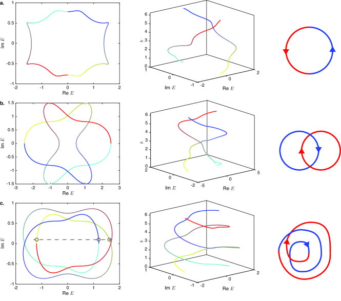
As the momentum varies from 0 to within the Brillouin zone, the trajectories of the two complex eigen energies may form knots in the 3D complex energy–momentum space. If we assume, without loss of generality that , then the two eigen energy bands may tangle with each other for up to times (e.g., if we set , the energy bands may tangle for zero, one, two, or three times) depending on the coupling parameters. Fig. 1 shows exemplary knot systems realized by the Hamiltonian in Eq. 1 with and in which the bands tangle once (Fig. 1a), twice (Fig. 1b), and three times (Fig. 1c). These correspond to the Unknot, Hopf link, and trefoil configurations, respectively. We can systematically describe these configurations via the Artins notation [89, 52],where a complex braiding with knots follows a sequence of band crossings, each of which can be described by the braiding word . Here, () denotes the case where the trajectory of the first energy strand crosses that of the second energy strand from the left (right) in the projection of the 3D trajectory onto the plane. The systems in Fig. 1a – c can thus be described by the braid words , , and , respectively.
Furthermore, the different types of knot configurations can be characterized by an integer topological number known as the braiding index , which is defined as [48]
| (3) |
where is the two-by-two identity matrix.
The magnitude of indicates the number of times that the eigen energy strands of wind or braid around each other in space, while its sign denotes the net handedness of the braiding. Using the fact that the determinant of a square matrix is equal to the product of its eigenvalues, introducing , and denoting the two eigenvalues of as , can be rewritten as
| (4) |
Because the Hamiltonian Eq. 1 is traceless, for this Hamiltonian can be interpreted as counting the number of times that its eigenvalues wind around the complex energy origin. For example, the leftmost plot in Fig. 1a shows that for this Unknot system, the two energy strands join together to form a single loop that winds in the counter-clockwise direction as increases (as is evident from the color coding of the energy strings where darker colors correspond to larger values), and hence corresponds to a braiding index of +1. For the Hopf link in Fig. 1b, the gray-red and yellow-blue bands each winds around the origin once in a clockwise manner, and hence collectively give rise to an overall braiding index of -2. For the trefoil in Fig. 1c, the gray-red and yellow-blue bands each winds around the origin for one and a half times in a counter-clockwise manner. (The fact that each band winds around the origin for one and a half times can be seen from, e.g., the yellow-blue line crossing a line slightly displaced above the real energy axis only once on the negative side but twice on the positive side, with the crossing points depicted by open circles in the left panel of Fig. 1c. ) The two bands therefore collectively give rise to a braiding index of -3. Interestingly, for two-band systems, each of the two energy strings begins and ends at the same value of complex energy at and , respectively, when is even, but when is odd, the start-point of one band coincides with the end-point of the other, and vice versa (so that the trajectory of the two bands collectively form a closed loop).
Beyond counting the number of times that the eigen energy strands wind around the origin on the complex energy plane, the braiding index has an alternative mathematical interpretation. Eq. (3) can be recast into the form of a contour integral over the complex unit circle in space:
| (5) |
Eq. (5) can be evaluated using the argument principle as , where is the number of zeros (poles) of enclosed inside the contour integral. From Eq. 2, . There are therefore poles of at within the complex unit circle due to the term. The zeros of occur when , the solutions of which are given by the following equation
| (6) |
where, , and when , i.e., the solutions of which are given by
| (7) |
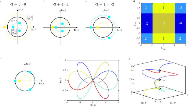
where, . Depending on the relative magnitudes of , , and , the () values of () may fall inside, on, or outside the complex unit circle. Neglecting for now the cases where the s or s lie exactly on the complex unit circle, the possible values of are thus , when , so that the s and s all lie outside the unit circle; 0, when , so that the s all lie within the unit circle while the s all lie outside (Fig. 2a); , when , , so that the s and s all lie inside the unit circle (Fig. 2b) ; and , so that the s all lie within the unit circle while the s all lie outside (Fig. 2c). This dependence of on the relative magnitudes of , , and results in the phase diagram shown in Fig. 2d where the boundaries between different values of the braiding indices are defined by the equations: and .
Let us now consider the case where the values of s (or values of s) fall on the unit circle on the complex plane (Fig. 2e), for which the value of () must necessarily fall on one of the phase boundaries between different values of . This is because the s and/or s have to pass through the unit circle, for the number of s solutions to that lie within the unit circle to change. The correspondence between the complex unit circle on the plane to real values of , i.e., means that there are , , or values of corresponding to zero energy on the PBC spectrum when only , only , or , respectively. Figs. 2f and 2g illustrate this for the specific case of . For the particular model in Eq. (1), the zeros of the also happen to be exceptional points because these zeros occur only when is rank-deficient and all the matrix elements in the left or right columns are zero.
III GBZ and NHSE variation in complex braiding configurations
We comment briefly on the relationship between the braiding index and the non-Hermitian skin effect (NHSE). In 1D systems, a winding number (or braiding index) [90] may be defined with respect to a reference energy as
| (8) |
The braiding index in Eq. (3) may be interpreted as a special case of the winding number where is set to , which for the model in Eq. (1) is equal to 0. The winding number may be visually determined from the PBC spectrum of a system provided that the individual bands can be separately identified and the direction of increasing indicated.
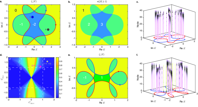
For example, in Fig. 3a the winding number at point A. because the bands indicated by the red and blue lines each winds around point A in a complete circle along the clockwise direction. In contrast, the winding number at point B, because point B falls completely outside the loop enclosed by the blue band and is enclosed only the red band, which winds around the point in the counter-clockwise direction.
The magnitude of the winding number is associated with the number of bulk NHSE states that exist in a semi-infinite system at , as explained shortly, while the sign of the winding number denotes whether it is a semi-infinite system that extends from 0 to (positive ) or a semi-infinite system that extends from to 0 that hosts such bulk NHSE states ([91]) The braiding index therefore indicates the number and localization of NHSE states that exist at in the semi-infinite system.
To further elucidate the relationship between the winding number and semi-infinite eigenstates, we examine these eigenstates more carefully. We consider first the eigenstates for a semi-infinite system that extends from to . We introduce the surrogate Hamiltonian [58] to the Hamiltonian in Eq. (1) as
| (9) |
where and is now allowed to be complex. If an eigenstate of the semi-infinite system at a given energy exists, the eigenstate can be generically written as a linear combination
| (10) |
where is the th value of for which one of the eigenvalues of is and is the corresponding eigenvector. The summation of from 1 to in Eq. (10) is due to the following considerations: The coupling between the B node of a unit cell and the A node of the th neighbor to its right represented by the term in Eq. (9) requires the A node component of , i.e. to satisfy the boundary conditions beyond the rightmost unit cell of the semi-infinite system at . A linear combination of linearly independent eigenvectors is therefore required in Eq. (10) to ensure that these constraints are always satisfied. Moreover, the corresponding values for these eigenvectors are required to satisfy to ensure that remains bounded as .
Whether such right-localized eigenstates exist in a semi-infinite system extending from to for a given therefore hinges on whether there are at least linearly independent eigenvectors of satisfying at that given . The characteristic equation for can be cast into the form of a th order polynomial , which in general has roots for the s, corresponding to linearly independent eigenvectors.
Now recall that the braiding index is where is the number of zeros of and is the number of poles of that lie within on the complex plane.As before, for simplicity, we first set aside the cases where any of the values lies exactly on the unit circle. The zeros of on the complex plane, are merely the values corresponding to . The number of s that lie within the complex unit circle on the plane (excluding the term), i.e. , is therefore because . Conversely, the number of s that lie outside the complex unit circle on the plane is . In particular, implies that there are values of that lie outside the complex plane with corresponding linearly independent eigenvectors. This is exactly the number of linearly independent eignvectors with required to constitute a right-localized semi-infinite NHSE eigenstate. A more negative value of implies that there is an excess number of eigenstates that may be used to construct a right-localized semi-infinite NHSE eigenstate. The fact that only such eigenstates are required out of the available ones implies that we can obtain linearly independent right-localized NHSE eigenstates in a semi-infinite system extending from to at . Here, denotes the number of different combinations of picking items out of a set of items. (Note that this differs from the interpretation in [91] where itself is interpreted to be the number of degenerate semi-infinite NHSE eigenstates.) In a similar manner, a positive value of implies that there are linearly independent left-localized NHSE eigenstates in a semi-infinite system extending from to at .
The above arguments that is correlated to the number of semi-infinite NHSE eigenstates at can be readily extended to the case of arbitary . Fig. 3b shows , i.e., the number of s for which corresponding to each value of in the parameter set in Fig. 3a, for which and . It can be readily verified by a comparison between Fig. 3a and 3b that the relation between the negative values of in Fig. 3a to in Fig. 3b is given by as discussed above. Further, the PBC spectrum coincides with the boundary lines between different values of . This is because changes in correspond to changes in the number of s within the complex unit circle on the plane, which are necessarily accompanied by s crossing the complex unit circle as is varied. A values that lies on the complex unit circle corresponds to a real value of in Eq. (1) and therefore lies on the PBC spectrum.
Let us label the s such that . Then, the general Brillouin zone (GBZ) of Eq. (1) for a system with open boundary conditions (OBC) in the thermodynamic limit is given by the loci of for which . Recall from the above discussion that the number of s that lie within the complex unit circle on the plane at energy is . For a value of that lies on the GBZ, a positive finite value of therefore implies that , which corresponds to a left-localized OBC NHSE state. Conversely, a negative value of in turn corresponds to a right-localized OBC NHSE state. Although strictly speaking, the GBZ condition applies only in the thermodynamic limit, the NHSE localization direction of a sufficiently long finite-sized chain follows that of the chain in the thermodynamic limit. In particular, a positive (negative) value of the braiding index implies that OBC NHSE states within the central area around bounded by the PBC spectrum are localized at the left (right) edge of the system. This is illustrated in Fig. 3c, which shows the eigenenergy and spatial density distribution for the eigenstates of a 40-node long finite system described by the Hamiltonian with the parameter set of Fig. 3a, b. As predicted by the negative signs of shown in Fig. 3a, most of the eigenstates are localized towards the right edge (large ) of the system, except for two topological zero modes (TZMs) that are localized towards the left edge (these TZMs are not described by the GBZ theory).
Apart from the TZMs, the NHSE localization direction may differ from that predicted by outside the central area on the complex energy plane around bounded by the PBC spectrum. Fig. 3d shows , the fraction of the 40 eigenstates of a 40 node-long system described by Eq. (1) localized closer to the left edge, as a function of and . A value of 1 indicates that all of the eigenstates are localized closer to the left edge while a proportion of 0 indicates that all of the eigenstates are localized closer to the right edge. In the regions at the four corners of the plot in Fig. 3d, there are regions at which deviates very slightly from 0. These slight deviations are due to TZMs that are localized at the left edge opposite to that of the NHSE eigenstates, as shown in Fig. 3c. Apart from the regions where all the eigenstates are localized to the right, bipolar localization, in which the NHSE eigenstates at different eigenenergies are localized at different edges of the system, occurs throughout much of the – parameter space. One example at is shown in Fig. 3e and f where Fig. 3f shows that the eigenstates in the central complex energy region around are localized to the left, consistent with , whereas the more numerous eigenstates in the complex side-lobes are localized towards the right, consistent with in these lobes, as shown in Fig. 3e.
IV Continuous jumps in braiding index via intra-unit cell coupling and onsite coupling
In the model in Eq. 1, there is a constraint in the braiding index in that it changes only in steps of or . This is because the () roots of () in Eq. (2) all have the same absolute values. We can remove this constraint by modifying the Hamiltonian with the introduction of a finite on-site potential, i.e.,
| (11) |
in which case the eigenenrgies now satisfy
| (12) |
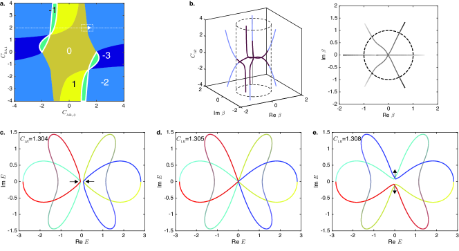
This results in a phase diagram for which all values of across the entire range of to appear, as shown in Fig. 4a. Due to the offset in Eq. 12, the values of that satisfy the condition will no longer have the same absolute values in general (Fig. 4b), thus removing the restriction on the change in to steps of or as was the case when . As mentioned previously, a change in will be accompanied by the appearance of a zero eigenenergy on the PBC spectrum since varies with the number of values at which the energy eigenvalues are 0 and . From Eq. 12, it can be seen that corresponds to an eigenenergy at which the two energy bands coincide with each other (Fig. 3d). As in Fig. 4)c–e is varied towards the boundary between two values (along the dotted line shown in Fig. 4a), the two bands begin to approach each other along the real energy axis (Fig. 4c). They then touch each other at at the transition point corresponding to the boundary line (Fig. 4d), and then drift apart along the imaginary energy axis (Fig. 4e) as is increased further. As the energy bands touch at the transition point, they swap partners, which in turn results in a change in the connectivity between the energy bands and accordingly, the number of times the two bands wind around . Consider the series of figures Fig. 4c–e. Before the transition (Fig. 4c), is less than 0 at the minimum value of , which results in the two bands being separated by a finite gap along the real energy axis; becomes 0 at the transition point, which results in the bands touching (Fig. 4d); and finally becomes positive after the transition point in Fig. 4e, which results in the two bands being separated by a finite gap along the imaginary energy axis.
V Impact of bidirectional asymmetric long range coupling on braiding profile
In the models introduced so far, the inter-unit cell A to B sublattice site coupling occurs only to the left ( ) while the B to A sublattice coupling occurs only to the right () term. This implies that the maximum value of that can occur is , i.e., the largest distance of the inter-unit cell coupling either along the left or right directions. We can further generalize the model to extend the range of possible values and attain a larger maximum value of for a given inter-cell coupling distance by incorporating inter-unit cell bidirectional coupling of both directions in both the A to B sublattice sites and vice versa. The corresponding Hamiltonian in the presence of this bidirectional coupling is given by
| (13) |
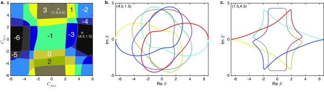
Fig. 5 shows an exemplary phase diagram for a system represented by Eq. (13) where , , and and two PBC spectra from the two extreme (positive and negative) values of and obtained when the terms with the largest positive and negative exponents in the upper right element of Eq. (13) are multplied with their counterparts in the lower left element. The presence of coupling along both the left and right directions in the two off-diagonal terms of implies that the exponents of the terms sum up in the characteristic equation for the eigenenergy , which is given by
| (14) |
In the characteristic equation, the exponents of now range from to . Correspondingly, for the example depicted in Fig. 5, the values of range from when all of the () values at fall outside the unit circle on the complex plane (Fig. 5b) to when all of the values fall within the unit circle. Compared to the earlier models with unidirectional couplings depicted in Figs. 2 to 4 for which resulted in the maximum value of being only 3,the presence of bidirectional coupling results in the doubling of the maximum value of to 6 even though the furthest inter-unit cell coupling is still maintained to the third neighbor.
VI Topological phase transition through exceptional curves
Two topologically distinct phases associated with different braiding index cannot be continuously transformed into one another without transiting through a vanishing bandgap state, at which point the braiding index changes its value. This transition signifies the presence of exceptional points (EPs) lying on the boundary between the two distinct phases. Specifically, all points lying on the phase boundaries between two distinguished knot configurations(see phase diagram of Fig. 2d and 4a) constitute EPs which are characterized by vanishing bandgap with real solution of .
To illustrate the phase transition via EPs, let us consider Eq. 1 and set without loss of generality. The modified Laplacian then reads
| (15) |
where, .Note that the band-gap of the two band non-Hermitian model can vanish in two possible ways. First, if the transition points lie at the phase boundary between two opposite handedness (i.e., the sign of the braiding index changes from positive sign to negative sign or vice versa) configurations, the two strings with undercross () configuration transforms into an overcross () configuration or vice versa, this sort of phase transition is referred as Type-2 phase transition which is accompanied by number of EPs (here we vary from to for simplicity). On the other hand, a second type of phase transition occurs when two strings change its braiding index number at the phase transition points while maintaining the same sign, so that the handedness of the braiding and the NHSE localization remains at the same edge. This is the so-called Type-1 phase transition, where an undercross (overcross) configuration remains undercross (overcross) in the braiding configuration. Type-1 transition is accompanied by a single EP.
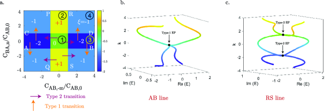
As an illustrative example, we consider a system with second-order long range coupling (i.e. setting in Eq. 15), and plot the corresponding phase diagram in Fig. 6. Clearly, the phase boundaries coincide with the and lines. Interestingly, the band diagrams corresponding to points lying on the lines PQ and RS (corresponding to ) host two exceptional points with Type-2 transition as there are only two real values of (i.e., for RS line, see Fig. 6c and for PQ line) which result in zero bandgap of Eq. 15. On the contrary, the band diagrams corresponding to lines AB and CD (corresponding to ) represents the Type-1 phase transition with a single exceptional point as there exist only a single real value of (i.e., for AB line, see Fig. 6b and for EF line) which satisfies the zero bandgap condition in Eq. 15. Thus a transition from unlink () to Hopf link with (unknot with ) phase constitutes a Type-2 (Type-1) transition (see Fig. 6a).
In general, Type-2 transition host number of EPs, for a system with long-range coupling of the order of , since there are real solutions of corresponding to zero bandgap. On the other hand, the Type-1 phase transition hosts only a single EP, regardless of the degree of the long-range coupling (i.e. ). We summarized the locations of Type-2 EPs and single Type-1 EP in the space for several example of long-range order in Table 1 (note that for simplicity we consider the values of within the range of to ).
| Order of long range coupling | Type-1 transition Transition through AB line | Type-1 transition Transition through EF line | Type-2 transition Transition through PQ line | Type-2 transition Transition through RS line |
VII Proposal for Topological Circuit Realization
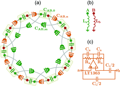
The intricate energy braiding described by the model in Eq. 1 can be implemented in a practical electrical circuit using an RLC configuration, as depicted in Fig. 7, for the specific parameter values of and under PBC configuration. For the corresponding OBC setup, the terminal couplings should be replaced with appropriate capacitors to ensure consistent total node admittance across all nodes (refer to Appendix A for detailed information). The behavior of this system is governed by Kirchhoff’s law, as expressed in Eq. (16).
| (16) |
Here, represents the current flowing into the node, denotes the circuit admittance between the and nodes, and is the voltage at the node. The circuit Laplacian, , is given by:
| (17) |
Where represents capacitor connected between node and , and are the grounding inductor connected to node . Applying Fourier transformation yields the space representation of the circuit Laplacian, as seen in Eq. (18):
| (18) |
Sub-lattice node A and B are grounded through inductors and respectively. is a bidirectional capacitor between node A and B, is an unidirectional capacitor from node A towards B and is an unidirectional capacitor from node B towards A (Fig. 7).
To realize any complex braiding phase, the system needs to be driven at the resonant frequency .
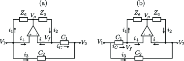
The real-space matrix formation of for both PBC and OBC can be found in Appendix A, supplemented by detailed derivations and circuit diagrams. Current-inversion negative impedance converters (INIC) topology, incorporating LT1363 Op-Amps, are employed to realize unidirectional capacitors (as shown in Fig 7(c)). To stabilize the Op-Amp output, a small capacitance () in the pico Farad range and a low-resistance () less than 1 k are connected in parallel. Since achieving a perfect unidirectional capacitance is challenging in practice, and are meticulously tuned and tested to attain the best possible unidirectional capacitance for the capacitors used in this study. Detailed results of the INIC optimization can be found in Appendix B.
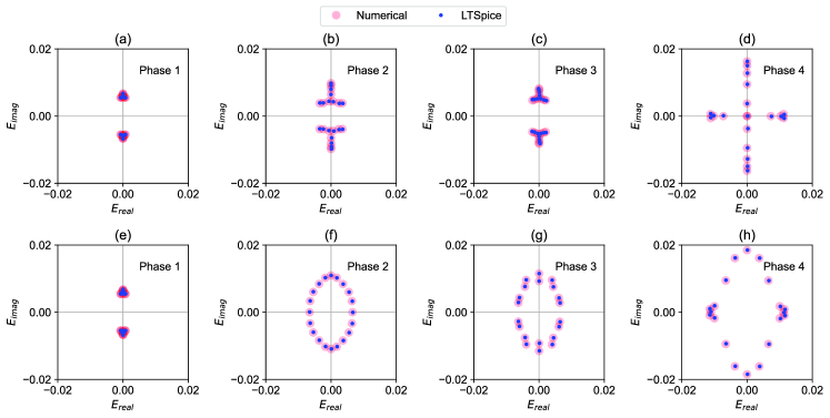
To illustrate the practical implementation of our proposed braiding scheme, four distinct braiding phases—referred to as phases 1 through 4 in Fig 6—have been selected for execution in the electrical circuit set-up. In the circuit implementation of the phases, we dynamically adjust the circuit parameters to demonstrate the versatility and adaptability of our proposed approach. More specifically, as the circuit is exposed to complex admittance eigen values with both positive and negative amplitudes, it is vulnerable to non-causal instabilities[31]. To prevent the system going unstable, we grounded each of the nodes with additional resistor to shift up the whole spectrum to have complex eigen values with no negative imaginary parts. This shifting, however, has no effect in realizing the braiding topologies this study is concerned about. Moreover, this ensures converged transient circuit simulation results as well. Careful numerical analysis was carried out to get the optimum value of which was chosen as . Also, parasitic resistance of was added to each inductors to mimic more real-world system. Table 2 lists all the chosen parameters for the four different phases.
| Phase | |||||
|---|---|---|---|---|---|
| 1 | 4.7 nF | 0.94 nF | 2 nF | 94.52 H | 112.28 H |
| 2 | 4.7 nF | 0.94 nF | 20 nF | 25.64 H | 112.28 H |
| 3 | 4.7 nF | 20 nF | 2 nF | 94.52 H | 25.64 H |
| 4 | 4.7 nF | 20 nF | 20 nF | 25.64 H | 25.64 H |
Interestingly, the complex energy admittance spectrum can be reconstructed from the circuit by applying current at each node and measuring the node voltages. This allows the construction of the circuit Green’s function. Subsequently, the inversion of this Green’s function provides the resulting circuit Laplacian. From the constructed circuit Laplacian, eigenvalues and eigen modes corresponding to the admittance spectrum and node voltage distribution can be calculated. Fig. 8 shows the complex admittance spectrum corresponding to the circuit of Fig. 7. The numerical results (red dots) are compared with LTSpice simulation results (blue dots), revealing that the electrical circuit setup can almost perfectly realize all the distinct phases of the complex braiding system. Although there are slight discrepancies between the numerical results and the circuit simulations, these mainly arise from the inclusion of parasitic resistance in the inductors and the imperfect unidirectional capacitance realized through the INIC, as discussed in detail in Appendices C-E. The necessary precautions for choosing parameters related to the INIC are thoroughly covered in these appendices to ensure the transient analysis of the circuit converges without causing the OpAmps to saturate. Furthermore, the effects of parasitics and disorder on the braiding configurations are discussed in Appendix D.
VIII Conclusion
In conclusion, we present a comprehensive analysis of complex energy braiding in 1D non-Hermitian systems with a general th order long-range asymmetrical coupling. Our work provides a new perspective on the emergence of novel topological phenomena induced by long-range coupling beyond the conventional nearest-neighbor interaction. By varying the coupling strengths, we demonstrate that the modified SSH model displays distinct knots and links topologies in the complex energy-momentum space under periodic boundary conditions (PBC). These topologies can be characterized by a new topological invariant, the braiding index. We establish a correlation between the braiding index and the zeros and poles of the characteristic polynomials, providing a novel insight to the topology of complex energy braiding.
Additionally, our work shows a deep connection between the braiding topology and eigen state localization due to the non-Hermitian skin effect (NHSE). We find that the NHSE can be localized at one or both terminals of the system, signifying the conventional or bipolar skin localization respectively, depending on the sign of the braiding index. Furthermore, we find that different complex energy braiding configurations with the same sign (opposite sign) can be transformed continuously through Type-1 (Type-2) phase transitions which traverse through single (multiple) exceptional points (EPs).
Finally, we propose a realistic experimental setup for realizing various braiding schemes in an RLC circuit. This circuit-based platform to realize braiding topology is readily implementable using basic circuit components and avoids the requirement for high-dimensional momentum space unlike most other proposed platforms [48, 54]. The proposed electrical circuit setup provides a promising platform for exploring the rich physics of complex energy braiding in non-Hermitian systems with non-reciprocal long-range coupling.
Acknowledgments
This work is supported by the Ministry of Education (MOE) Tier-II Grant MOE-T2EP50121-0014 (NUS Grant No. A-8000086-01-00), and MOE Tier-I FRC Grant (NUS Grant No. A-8000195-01-00).
References
- Ashida et al. [2020] Y. Ashida, Z. Gong, and M. Ueda, Non-hermitian physics, Adv. Phys. 69, 249 (2020).
- Bergholtz et al. [2021] E. J. Bergholtz, J. C. Budich, and F. K. Kunst, Exceptional topology of non-hermitian systems, Rev. Mod. Phys. 93, 015005 (2021).
- Gong et al. [2018a] Z. Gong, Y. Ashida, K. Kawabata, K. Takasan, S. Higashikawa, and M. Ueda, Topological phases of non-hermitian systems, Phys. Rev. X 8, 031079 (2018a).
- Leykam et al. [2017] D. Leykam, K. Y. Bliokh, C. Huang, Y. D. Chong, and F. Nori, Edge modes, degeneracies, and topological numbers in non-hermitian systems, Phys. Rev. lett. 118, 040401 (2017).
- Rafi-Ul-Islam et al. [2022a] S. M. Rafi-Ul-Islam, Z. B. Siu, H. Sahin, C. H. Lee, and M. B. A. Jalil, Critical hybridization of skin modes in coupled non-hermitian chains, Phys. Rev. Res. 4, 013243 (2022a).
- Yokomizo and Murakami [2019] K. Yokomizo and S. Murakami, Non-bloch band theory of non-hermitian systems, Phys. Rev. lett. 123, 066404 (2019).
- El-Ganainy et al. [2019] R. El-Ganainy, M. Khajavikhan, D. N. Christodoulides, and S. K. Ozdemir, The dawn of non-hermitian optics, Commun. Phys. 2, 37 (2019).
- Cao et al. [2020] W. Cao, X. Lu, X. Meng, J. Sun, H. Shen, and Y. Xiao, Reservoir-mediated quantum correlations in non-hermitian optical system, Phys. Rev. Lett. 124, 030401 (2020).
- Zhang et al. [2018] Z. Zhang, D. Ma, J. Sheng, Y. Zhang, Y. Zhang, and M. Xiao, Non-hermitian optics in atomic systems, J. Phys. B: Atom, Mol. Opt. Phys. 51, 072001 (2018).
- Feng et al. [2017] L. Feng, R. El-Ganainy, and L. Ge, Non-hermitian photonics based on parity–time symmetry, Nat. Photon. 11, 752 (2017).
- Pan et al. [2018] M. Pan, H. Zhao, P. Miao, S. Longhi, and L. Feng, Photonic zero mode in a non-hermitian photonic lattice, Nat. Commun. 9, 1308 (2018).
- Longhi et al. [2015] S. Longhi, D. Gatti, and G. D. Valle, Robust light transport in non-hermitian photonic lattices, Sci. Rep. 5, 1 (2015).
- Midya et al. [2018] B. Midya, H. Zhao, and L. Feng, Non-hermitian photonics promises exceptional topology of light, Nat. Commun. 9, 2674 (2018).
- Ghatak et al. [2020] A. Ghatak, M. Brandenbourger, J. Van Wezel, and C. Coulais, Observation of non-hermitian topology and its bulk–edge correspondence in an active mechanical metamaterial, Proc. Nat. Aca. Sci. 117, 29561 (2020).
- Hou et al. [2020] J. Hou, Z. Li, X.-W. Luo, Q. Gu, and C. Zhang, Topological bands and triply degenerate points in non-hermitian hyperbolic metamaterials, Phys. Rev. Lett. 124, 073603 (2020).
- Zhou and Zhang [2020] D. Zhou and J. Zhang, Non-hermitian topological metamaterials with odd elasticity, Phys. Rev. Res. 2, 023173 (2020).
- Rosenthal et al. [2018] E. I. Rosenthal, N. K. Ehrlich, M. S. Rudner, A. P. Higginbotham, and K. W. Lehnert, Topological phase transition measured in a dissipative metamaterial, Phys. Rev. B 97, 220301 (2018).
- Fring and Taira [2020a] A. Fring and T. Taira, Pseudo-hermitian approach to goldstone’s theorem in non-abelian non-hermitian quantum field theories, Phys. Rev. D 101, 045014 (2020a).
- Moiseyev [2011] N. Moiseyev, Non-Hermitian quantum mechanics (Cambridge University Press, 2011).
- Fring and Taira [2020b] A. Fring and T. Taira, Goldstone bosons in different pt-regimes of non-hermitian scalar quantum field theories, Nucl. Phys. B 950, 114834 (2020b).
- Rafi-Ul-Islam et al. [2021a] S. M. Rafi-Ul-Islam, Z. B. Siu, and M. B. A. Jalil, Non-hermitian topological phases and exceptional lines in topolectrical circuits, New J. Phys. 23, 033014 (2021a).
- Hofmann et al. [2020] T. Hofmann, T. Helbig, F. Schindler, N. Salgo, M. Brzezińska, M. Greiter, T. Kiessling, D. Wolf, A. Vollhardt, A. Kabaši, et al., Reciprocal skin effect and its realization in a topolectrical circuit, Phys. Rev. Res. 2, 023265 (2020).
- Zhang et al. [2023a] X. Zhang, B. Zhang, H. Sahin, Z. B. Siu, S. M. Rafi-Ul-Islam, J. F. Kong, B. Shen, M. B. A. Jalil, R. Thomale, and C. H. Lee, Anomalous fractal scaling in two-dimensional electric networks, Commun. Phys. 6, 151 (2023a).
- Sahin et al. [2023] H. Sahin, Z. B. Siu, S. M. Rafi-Ul-Islam, J. F. Kong, M. B. A. Jalil, and C. H. Lee, Impedance responses and size-dependent resonances in topolectrical circuits via the method of images, Phys. Rev. B 107, 245114 (2023).
- Rafi-Ul-Islam et al. [2020a] S. M. Rafi-Ul-Islam, Z. Bin Siu, and M. B. A. Jalil, Topoelectrical circuit realization of a weyl semimetal heterojunction, Commun. Phys. 3, 72 (2020a).
- Rafi-Ul-Islam et al. [2020b] S. M. Rafi-Ul-Islam, Z. B. Siu, C. Sun, and M. B. A. Jalil, Realization of weyl semimetal phases in topoelectrical circuits, New J. Phys. 22, 023025 (2020b).
- Rafi-Ul-Islam et al. [2020c] S. M. Rafi-Ul-Islam, Z. B. Siu, and M. B. A. Jalil, Anti-klein tunneling in topoelectrical weyl semimetal circuits, Appl. Phys. Lett. 116 (2020c).
- Rafi-Ul-Islam et al. [2023a] S. M. Rafi-Ul-Islam, Z. B. Siu, H. Sahin, and M. B. A. Jalil, Valley hall effect and kink states in topolectrical circuits, Phys. Rev. Res. 5, 013107 (2023a).
- Rafi-Ul-Islam et al. [2021b] S. M. Rafi-Ul-Islam, Z. B. Siu, and M. B. A. Jalil, Topological phases with higher winding numbers in nonreciprocal one-dimensional topolectrical circuits, Phys. Rev. B 103, 035420 (2021b).
- Zou et al. [2021] D. Zou, T. Chen, W. He, J. Bao, C. H. Lee, H. Sun, and X. Zhang, Observation of hybrid higher-order skin-topological effect in non-hermitian topolectrical circuits, Nat. Commun. 12, 7201 (2021).
- Helbig et al. [2020] T. Helbig, T. Hofmann, S. Imhof, M. Abdelghany, T. Kiessling, L. Molenkamp, C. Lee, A. Szameit, M. Greiter, and R. Thomale, Generalized bulk–boundary correspondence in non-hermitian topolectrical circuits, Nat. Phys. 16, 747 (2020).
- Rafi-Ul-Islam et al. [2022b] S. M. Rafi-Ul-Islam, Z. B. Siu, H. Sahin, C. H. Lee, and M. B. A. Jalil, System size dependent topological zero modes in coupled topolectrical chains, Phys. Rev. B 106, 075158 (2022b).
- Lee et al. [2018] C. H. Lee, S. Imhof, C. Berger, F. Bayer, J. Brehm, L. W. Molenkamp, T. Kiessling, and R. Thomale, Topolectrical circuits, Commun. Phys. 1, 39 (2018).
- Rafi-Ul-Islam et al. [2022c] S. M. Rafi-Ul-Islam, H. Sahin, Z. B. Siu, and M. B. A. Jalil, Interfacial skin modes at a non-hermitian heterojunction, Phys. Rev. Res. 4, 043021 (2022c).
- Rafi-Ul-Islam et al. [2022d] S. M. Rafi-Ul-Islam, Z. B. Siu, H. Sahin, and M. B. A. Jalil, Type-ii corner modes in topolectrical circuits, Phys. Rev. B 106, 245128 (2022d).
- Martinez Alvarez et al. [2018] V. Martinez Alvarez, J. Barrios Vargas, M. Berdakin, and L. Foa Torres, Topological states of non-hermitian systems, Eur. Phys. J. Spec. Top. 227, 1295 (2018).
- Ghatak and Das [2019] A. Ghatak and T. Das, New topological invariants in non-hermitian systems, J. Phys. Condens. Matt. 31, 263001 (2019).
- Rafi-Ul-Islam et al. [2020d] S. M. Rafi-Ul-Islam, Z. B. Siu, C. Sun, and M. B. A. Jalil, Strain-controlled current switching in weyl semimetals, Phys. Rev. Appl. 14, 034007 (2020d).
- Lee et al. [2014] T. E. Lee, F. Reiter, and N. Moiseyev, Entanglement and spin squeezing in non-hermitian phase transitions, Phys. Rev. Lett. 113, 250401 (2014).
- Lee and Thomale [2019] C. H. Lee and R. Thomale, Anatomy of skin modes and topology in non-hermitian systems, Phys. Rev. B 99, 201103 (2019).
- Li and Lee [2022] L. Li and C. H. Lee, Non-hermitian pseudo-gaps, Sci. Bull. 67, 685 (2022).
- Rafi-Ul-Islam et al. [2022e] S. M. Rafi-Ul-Islam, Z. B. Siu, H. Sahin, C. H. Lee, and M. B. A. Jalil, Unconventional skin modes in generalized topolectrical circuits with multiple asymmetric couplings, Phys. Rev. Res. 4, 043108 (2022e).
- Kawabata et al. [2020a] K. Kawabata, N. Okuma, and M. Sato, Non-bloch band theory of non-hermitian hamiltonians in the symplectic class, Phys. Rev. B 101, 195147 (2020a).
- Zhang et al. [2020] K. Zhang, Z. Yang, and C. Fang, Correspondence between winding numbers and skin modes in non-hermitian systems, Phys. Rev. Lett. 125, 126402 (2020).
- Liu et al. [2019] T. Liu, Y.-R. Zhang, Q. Ai, Z. Gong, K. Kawabata, M. Ueda, and F. Nori, Second-order topological phases in non-hermitian systems, Phys. Rev. Lett. 122, 076801 (2019).
- Hamazaki et al. [2019] R. Hamazaki, K. Kawabata, and M. Ueda, Non-hermitian many-body localization, Phys. Rev. Lett. 123, 090603 (2019).
- Hu and Zhao [2021] H. Hu and E. Zhao, Knots and non-hermitian bloch bands, Phys. Rev. lett. 126, 010401 (2021).
- Wang et al. [2021a] K. Wang, A. Dutt, C. C. Wojcik, and S. Fan, Topological complex-energy braiding of non-hermitian bands, Nature 598, 59 (2021a).
- Lee et al. [2020] C. H. Lee, A. Sutrisno, T. Hofmann, T. Helbig, Y. Liu, Y. S. Ang, L. K. Ang, X. Zhang, M. Greiter, and R. Thomale, Imaging nodal knots in momentum space through topolectrical circuits, Nat. Commun. 11, 4385 (2020).
- Li and Mong [2021] Z. Li and R. S. Mong, Homotopical characterization of non-hermitian band structures, Phys. Rev. B 103, 155129 (2021).
- Ezawa [2019] M. Ezawa, Braiding of majorana-like corner states in electric circuits and its non-hermitian generalization, Phys. Rev. B 100, 045407 (2019).
- Hu et al. [2022] H. Hu, S. Sun, and S. Chen, Knot topology of exceptional point and non-hermitian no-go theorem, Phys. Rev. Res. 4, L022064 (2022).
- Zhang et al. [2023b] Q. Zhang, Y. Li, H. Sun, X. Liu, L. Zhao, X. Feng, X. Fan, and C. Qiu, Observation of acoustic non-hermitian bloch braids and associated topological phase transitions, Phys. Rev. Lett. 130, 017201 (2023b).
- Li et al. [2022] Y. Li, Y. Chen, and X. Yang, Topological energy braiding of the non-bloch bands, ArXiv preprint arXiv:2204.12857 (2022).
- Okuma et al. [2020a] N. Okuma, K. Kawabata, K. Shiozaki, and M. Sato, Topological origin of non-hermitian skin effects, Phys. Rev. Lett. 124, 086801 (2020a).
- Siu et al. [2023] Z. B. Siu, S. M. Rafi-Ul-Islam, and M. B. A. Jalil, Terminal-coupling induced critical eigenspectrum transition in closed non-hermitian loops, Sci. Rep. 13, 22770 (2023).
- Rafi-Ul-Islam et al. [2024a] S. M. Rafi-Ul-Islam, Z. B. Siu, M. S. H. Razo, and M. B. A. Jalil, Saturation dynamics in non-hermitian topological sensing systems, ArXiv Preprint ArXiv:2406.19629 (2024a).
- Li et al. [2020] L. Li, C. H. Lee, S. Mu, and J. Gong, Critical non-hermitian skin effect, Nat. Commun. 11, 5491 (2020).
- Rafi-Ul-Islam et al. [2024b] S. M. Rafi-Ul-Islam, Z. B. Siu, H. Sahin, M. S. H. Razo, and M. B. A. Jalil, Twisted topology of non-hermitian systems induced by long-range coupling, Phys. Rev. B 109, 045410 (2024b).
- Longhi [2019] S. Longhi, Probing non-hermitian skin effect and non-bloch phase transitions, Phys. Rev. Res. 1, 023013 (2019).
- Song et al. [2019] F. Song, S. Yao, and Z. Wang, Non-hermitian skin effect and chiral damping in open quantum systems, Phys. Rev. Lett. 123, 170401 (2019).
- Kawabata et al. [2020b] K. Kawabata, M. Sato, and K. Shiozaki, Higher-order non-hermitian skin effect, Phys. Rev. B 102, 205118 (2020b).
- Zhang et al. [2021a] X. Zhang, Y. Tian, J.-H. Jiang, M.-H. Lu, and Y.-F. Chen, Observation of higher-order non-hermitian skin effect, Nat. Commun. 12, 5377 (2021a).
- Zhang et al. [2022] K. Zhang, Z. Yang, and C. Fang, Universal non-hermitian skin effect in two and higher dimensions, Nat. Commun. 13, 2496 (2022).
- Kawabata et al. [2019] K. Kawabata, T. Bessho, and M. Sato, Classification of exceptional points and non-hermitian topological semimetals, Phys. Rev. Lett. 123, 066405 (2019).
- Minganti et al. [2019] F. Minganti, A. Miranowicz, R. W. Chhajlany, and F. Nori, Quantum exceptional points of non-hermitian hamiltonians and liouvillians: The effects of quantum jumps, Phys. Rev. A 100, 062131 (2019).
- Hu et al. [2017] W. Hu, H. Wang, P. P. Shum, and Y. D. Chong, Exceptional points in a non-hermitian topological pump, Phys. Rev. B 95, 184306 (2017).
- Parto et al. [2021] M. Parto, Y. G. Liu, B. Bahari, M. Khajavikhan, and D. N. Christodoulides, Non-hermitian and topological photonics: optics at an exceptional point, Nanophotonics 10, 403 (2021).
- Rafi-Ul-Islam et al. [2022f] S. M. Rafi-Ul-Islam, Z. B. Siu, H. Sahin, and M. B. A. Jalil, Valley and spin quantum hall conductance of silicene coupled to a ferroelectric layer, Front. Phys. 10, 1021192 (2022f).
- Rafi-Ul-Islam et al. [2023b] S. M. Rafi-Ul-Islam, Z. B. Siu, H. Sahin, and M. B. A. Jalil, Conductance modulation and spin/valley polarized transmission in silicene coupled with ferroelectric layer, J. Magn. Magn. Mater. 571, 170559 (2023b).
- Rafi-Ul-Islam et al. [2024c] S. M. Rafi-Ul-Islam, Z. B. Siu, H. Sahin, and M. B. A. Jalil, Chiral surface and hinge states in higher-order weyl semimetallic circuits, Phys. Rev. B 109, 085430 (2024c).
- Sun et al. [2019] C. Sun, J. Deng, S. M. Rafi-Ul-Islam, G. Liang, H. Yang, and M. B. A. Jalil, Field-free switching of perpendicular magnetization through spin hall and anomalous hall effects in ferromagnet–heavy-metal–ferromagnet structures, Phys. Rev. Appl. 12, 034022 (2019).
- Sun et al. [2020] C. Sun, S. M. Rafi-Ul-Islam, H. Yang, and M. B. A. Jalil, Spin nernst and anomalous nernst effects and their signature outputs in ferromagnet/nonmagnet heterostructures, Physical Review B 102, 214419 (2020).
- Malciu et al. [2018] C. Malciu, L. Mazza, and C. Mora, Braiding majorana zero modes using quantum dots, Phys. Rev. B 98, 165426 (2018).
- Homeier et al. [2021] L. Homeier, C. Schweizer, M. Aidelsburger, A. Fedorov, and F. Grusdt, Z 2 lattice gauge theories and kitaev’s toric code: A scheme for analog quantum simulation, Phys. Rev. B 104, 085138 (2021).
- Sekania et al. [2017] M. Sekania, S. Plugge, M. Greiter, R. Thomale, and P. Schmitteckert, Braiding errors in interacting majorana quantum wires, Phys. Rev. B 96, 094307 (2017).
- Ezawa [2020] M. Ezawa, Non-abelian braiding of majorana-like edge states and topological quantum computations in electric circuits, Phys. Rev. B 102, 075424 (2020).
- Backens et al. [2017] S. Backens, A. Shnirman, Y. Makhlin, Y. Gefen, J. E. Mooij, and G. Schön, Emulating majorana fermions and their braiding by ising spin chains, Phys. Rev. B 96, 195402 (2017).
- Pahomi et al. [2020] T. E. Pahomi, M. Sigrist, and A. A. Soluyanov, Braiding majorana corner modes in a second-order topological superconductor, Phys. Rev. Res. 2, 032068 (2020).
- Levin and Gu [2012] M. Levin and Z.-C. Gu, Braiding statistics approach to symmetry-protected topological phases, Phys. Rev. B 86, 115109 (2012).
- Noh et al. [2020] J. Noh, T. Schuster, T. Iadecola, S. Huang, M. Wang, K. P. Chen, C. Chamon, and M. C. Rechtsman, Braiding photonic topological zero modes, Nat. Phys. 16, 989 (2020).
- Iadecola et al. [2016] T. Iadecola, T. Schuster, and C. Chamon, Non-abelian braiding of light, Phys. Rev. Lett. 117, 073901 (2016).
- Barlas and Prodan [2020] Y. Barlas and E. Prodan, Topological braiding of non-abelian midgap defects in classical metamaterials, Phys. Rev. Lett. 124, 146801 (2020).
- Nayak et al. [2008] C. Nayak, S. H. Simon, A. Stern, M. Freedman, and S. D. Sarma, Non-abelian anyons and topological quantum computation, Rev. Mod. Phys. 80, 1083 (2008).
- Wang et al. [2021b] K. Wang, A. Dutt, K. Y. Yang, C. C. Wojcik, J. Vučković, and S. Fan, Generating arbitrary topological windings of a non-hermitian band, Science 371, 1240 (2021b).
- Patil et al. [2022] Y. S. Patil, J. Höller, P. A. Henry, C. Guria, Y. Zhang, L. Jiang, N. Kralj, N. Read, and J. G. Harris, Measuring the knot of non-hermitian degeneracies and non-commuting braids, Nature 607, 271 (2022).
- Zhang et al. [2021b] L. Zhang, Y. Yang, Y. Ge, Y.-J. Guan, Q. Chen, Q. Yan, F. Chen, R. Xi, Y. Li, D. Jia, et al., Acoustic non-hermitian skin effect from twisted winding topology, Nat. Commun. 12, 6297 (2021b).
- Zhang and Song [2019] X. Zhang and Z. Song, Partial topological zak phase and dynamical confinement in a non-hermitian bipartite system, Phys. Rev. A 99, 012113 (2019).
- Rehren and Schroer [1989] K.-H. Rehren and B. Schroer, Einstein causality and artin braids, Nucl. Phys. B 312, 715 (1989).
- Okuma et al. [2020b] N. Okuma, K. Kawabata, K. Shiozaki, and M. Sato, Topological origin of non-hermitian skin effects, Phys. Rev. Lett. 124, 086801 (2020b).
- Gong et al. [2018b] Z. Gong, Y. Ashida, K. Kawabata, K. Takasan, S. Higashikawa, and M. Ueda, Topological phases of non-hermitian systems, Phys. Rev. X 8, 031079 (2018b).
- Wang et al. [2022] K. Wang, A. Dutt, C. C. Wojcik, and S. Fan, Realization of topological complex-energy braids and knots of non-hermitian bands, in CLEO: QELS_Fundamental Science (Optica Publishing Group, 2022) pp. JW4A–1.
Appendix A Circuit Laplacian Formation
In this section, we undertake a detailed derivation of the circuit Laplacian specifically for the case where and , considering a circuit with 10 unit cells, corresponding to 20 nodes. Our objective is to apply Kirchhoff’s Current Law (KCL) as expressed in Eq. 16 to every node within the circuit illustrated in Fig. 7.
| Node 1: | |
|---|---|
| Node 2: | |
| Node 3: | |
| Node 4: | |
| Node 19: | |
| Node 20: |
In matrix format, we can write
| (19) |
where and are the diagonal admittances. The real-space representation of the model in Eq. 1 mirrors 19, with the exception of the diagonal terms. By exciting the circuit at the resonant frequency , we can effectively eliminate these diagonal terms.
To realize the OBC system, the capacitors coupling the two ends must be removed, meaning the terms highlighted in red in Eq. 19 will be replaced by zero. Subsequently, when the Laplacian matrix is multiplied by the complex frequency , the real spectrum of the Laplacian corresponds to the imaginary spectrum of Eq. 1, and vice versa.
Appendix B Unidirectional Capacitor
Achieving unidirectional coupling in an electrical circuit involves the utilization of a unidirectional capacitor, which can be effectively implemented through a negative impedance converter with current inversion (INIC). The circuit configuration is depicted in Fig. 9. Employing this INIC setup enables the realization of a unidirectional capacitor.
To establish a unidirectional capacitance, denoted as , between node 1 and node 2, it is imperative to ensure that the capacitance from node 1 to 2 is , while the capacitance from node 2 to 1 is effectively zero. The INIC setup, as illustrated in Fig. 9, facilitates the creation of this unidirectional capacitance by setting in Fig. 9a. For the purpose of stabilizing the Op-Amp output, a capacitor is added in parallel with a resistor . Together, these components form an impedance denoted as . The unidirectionality of capacitive reactance, denoted as , is achieved through this setup.
B.1 Zero-Capacitance
In this subsection, we delve into the intricacies of achieving nearly unidirectional capacitive coupling by approaching zero capacitance in one direction. In Fig. 9(a), we make the assumption of the Op-Amp’s linear operation, and due to its very high open-loop gain, we can consider the voltages at its inverting and non-inverting terminals to be equal, i.e., . This implies . Additionally, owing to the Op-Amp’s extremely high input impedance, the input currents at both inverting and non-inverting terminals are approximately zero, i.e., .
Now, the current from node 1 to the output terminal of the Op-Amp is given by:
| (20) |
Similarly, the current from the output of the Op-Amp to the inverting terminal will be as . Since the current going to the Op-Amp through the inverting terminal, , is zero, the same will flow through , i.e., .
| (21) |
where is the capacitive reactance of capacitor at frequency .
From (20):
This results in an equivalent negative capacitor. If another capacitor with impedance is added in parallel, the total equivalent capacitance will be approximately . Choosing leads to an equivalent capacitance of approximately zero.
B.2 Non-zero Capacitance
In the scenario where we reverse the polarity of the voltage applied to the same circuit, as illustrated in Fig. (9)(b), positive capacitance can be achieved. Utilizing the same analysis as before, we consider and . Consequently, the current flowing through is given by:
In this case, we obtain a positive capacitive reactance . Introducing a parallel capacitor results in a total capacitance of .
B.3 Testing Unidirectional Capacitance
To test the unidirectional capacitance, we setup a typical low-pass filter and used our unidirectional capacitor as a test capacitance. In Fig. 10(a) we tested the zero capacitance and by reversing the polarity of the capacitor in Fig. 10(b) we test non-zero capacitance.
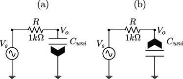
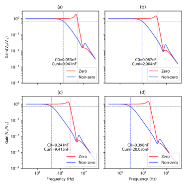
Fig. 11 shows LTSpice simulation results of testing our unidirectional capacitors in a low pass filter configuration. From the voltage gain(), we calculated the 3dB frequency of a low pass filter as . We used as a test resistor. For zero (blue line) and non-zero(red line) configurations, we found non-zero capacitances are 17, 23, 39 and 50 times higher than the zero capacitances.
Appendix C Constraints on Knot Types Achievable in Our Setup
In our model, not all types of knot configurations can be realized; only knots with an unknotting number of one can be achieved. The unknotting number, a concept from knot theory, measures the minimum number of crossing changes needed to transform a given knot into the simplest possible knot, known as the unknot (a simple loop). In the context of our model with two bands in a 1D setup containing long-range coupling, it is indeed true that only twist knots with an unknotting number of one can be realized. For example, in the case of a Hopf link or a trefoil knot configuration, only a single crossing needs to be changed to transform the knot configuration into an unknot configuration. Furthermore, it is true that knots with larger unknotting numbers (such as the Cinquefoil knot with an unknotting number of two) are not possible in our current two-band model, as each band must have a unique complex value at each -point.
Appendix D Robustness of the knot configurations against disorder
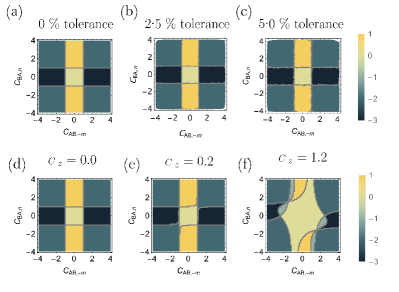
Our system demonstrates robustness against small parasitic effects. To verify this, we varied the components within a 5% tolerance of Eq. 1 and plotted the topological knot phase diagram in Fig.12a-c, which showed a profile almost identical to the original one. Thus, the knot configuration is quite protected against small parasitic variations. However, the situation changes when a term is included in the Hamiltonian. If we rewrite the Hamiltonian in Eq. 1 with a mass term as
| (22) |
where, is the third Pauli matrix and corresponds to the mass-like term in the Hamiltonian, this term breaks the chiral symmetry of the Hamiltonian. In the presence of a small mass term (i.e., ), the braiding index phase diagram does not change significantly (see Fig.12d). Therefore, the complex braiding/knot configuration remains protected. However, with a larger mass-like term (i.e., ), the braiding index phase diagram changes a lot and the region with zero knot index (unknotting phase) expands in the parameter plane, as shown in Fig.12f, while retaining other knot configurations with non-zero knot index in smaller range of parameters. As a result, knot structures convert to an unknot configuration across the wider parameter regime. Thus, knot structures are still protected in the presence of a large chiral symmetry-breaking term but at the different coupling parameters range.
Appendix E Stability of the Proposed Electric Circuit Network
In this section, we discuss some important points regarding the stability of the proposed electric circuit network. Indeed, the use of active elements such as operational amplifiers (OpAmps) in a negative impedance converter configuration to achieve unidirectional couplings can introduce stability concerns.
To address this, we conducted additional analyses beyond the steady-state AC simulations originally performed with LTSpice. Specifically, we examined the time dynamics of the system to assess the stability of the circuit. Our findings indicate that the eigenvalues of the Laplacian with a negative imaginary part can indeed lead to exponentially increasing time evolution of the corresponding eigenstates, potentially causing instability. For systems with periodic boundary conditions, this issue is particularly critical as even slightly unstable modes can diverge due to the loop feedback of the boundary conditions. To mitigate this risk, careful design of the OpAmp circuit is essential, including the implementation of feedback mechanisms to ensure stability.
Additionally, we have outlined the steps taken to ensure stability in the possible experimental setup, including the design parameters and feedback mechanisms used to counteract potential instabilities. To prevent the system from going unstable due to non-causal instability, we added an additional resistor to each node to shift the entire admittance spectrum upward such that no complex eigenvalues have negative imaginary parts. This adjustment does not alter the eigenstate profile, allowing us to still observe the same braiding patterns. With these changes in the circuit design, time domain analysis of the system converges, and the system becomes stable.
Furthermore, to achieve almost real-like outputs from circuit simulations, we added a parasitic resistance of to each inductor. While this inclusion of parasitic resistance results in slight mismatches from the numerical results, as shown in Fig. 8 of the main manuscript, the circuit now provides almost real outputs that are stable.