The $\mathcal{T}\kern-1.19995pt\mathcal{R}\kern-1.19995pt\mathcal{O}\kern-1.19995pt\mathcal{Y}$project
III. Exploring co-orbitals around low-mass stars

Abstract

Context. Co-orbital objects, also known as trojans, are frequently found in simulations of planetary system formation. In these configurations, a planet shares its orbit with other massive bodies. It is still unclear why there have not been any co-orbitals discovered thus far in exoplanetary systems (exotrojans) or even pairs of planets found in such a 1:1 mean motion resonance. Reconciling observations and theory is an open subject in the field.

Aims. The main objective of the $\mathcal{T}\kern-1.19995pt\mathcal{R}\kern-1.19995pt\mathcal{O}\kern-1.19995pt\mathcal{Y}$project is to conduct an exhaustive search for exotrojans using diverse observational techniques. In this work, we analyze the radial velocity time series informed by transits, focusing the search around low-mass stars.

Methods. We employed the $\alpha$-test method on confirmed planets searching for shifts between spectral and photometric mid-transit times. This technique is sensitive to mass imbalances within the planetary orbit, allowing us to identify non-negligible co-orbital masses.

Results. Among the 95 transiting planets examined, we find one robust exotrojan candidate with a significant 3-$\sigma$ detection. Additionally, 25 exoplanets show compatibility with the presence of exotrojan companions at a 1-$\sigma$ level, requiring further observations to better constrain their presence. For two of those weak candidates, we find dimmings in their light curves within the predicted Lagrangian region. We established upper limits on the co-orbital masses for either the candidates and null detections.

Conclusions. Our analysis reveals that current high-resolution spectrographs effectively rule out co-orbitals more massive than Saturn around low-mass stars. This work points out to dozens of targets that have the potential to better constraint their exotrojan upper mass limit with dedicated radial velocity observations. We also explored the potential of observing the secondary eclipses of the confirmed exoplanets in our sample to enhance the exotrojan search, ultimately leading to a more accurate estimation of the occurrence rate of exotrojans.

1 Introduction

Co-orbital configurations abound in the Solar System, where two massive bodies share their orbital path around the star. However, their detection beyond our system remains elusive. Two different mechanisms have been proposed to explain their formation, which are also expected to apply to exoplanetary systems: 1) in situ from the same material as protoplanets (e.g., Beaugé et al. 2007) or 2) via resonant captures at more advanced stages (e.g., 2018camN). Recent ALMA observations of three protoplanetary disks may be the first observational hints in favor of their in situ assembly, since they exhibit substructures that could be interpreted as an accumulation of material within the L₄ & L₅ Lagrangian points of forming planets. In HD 163296 and LkCa 15, it has been found asymmetric emissions with shapes that are reminiscent of the dust traps that appear in the process of trojan formation, as seen in hydrodynamical simulations (Isella et al. 2018; Long et al. 2022). An equivalent unresolved emission was found also in PDS 70 promisingly matching the L₅ region of the protoplanet PDS 70 b (Balsalobre-Ruza et al. 2023).

As posited by Laughlin & Chambers (2002), two co-orbiting similar-mass planets can be stable in the long term. Such stability remains possible as long as the total mass of the planet and the trojan does not surpass 3.7% of their host star mass (i.e., $[\rm{m_{p}}+\rm{m_{t}}]/M_{\star}<1/27$). This constraint allows for multiple co-orbital configurations to remain longstanding, including pairs of equal-mass planets. Although this exotic configuration is absent in the Solar System, its theoretically hypothesized stability encourages the detectability of exotrojan pairs for the first time. Such co-orbital systems could be accessible using current instrumentation, even from the ground (e.g., Ford & Gaudi 2006; Haghighipour et al. 2013; Hippke & Angerhausen 2015).

The absence of detections in exotrojan studies so far may be attributed to two non-exclusive reasons: i) co-orbital configurations might get disrupted earlier than theoretically predicted and ii) observational biases, as degeneracies with simpler configurations for the observed signals (see e.g., Giuppone et al. 2012; Goździewski & Konacki 2006) or the existence of transit timing variations (hereafter TTVs, e.g., García-Melendo & López-Morales 2011; Leleu et al. 2021b) can prevent their detection. Dedicated studies are therefore needed to ascertain the presence of the 1:1 mean motion resonance (MMR) in planetary system. This is the purpose of the $\mathcal{T}\kern-1.19995pt\mathcal{R}\kern-1.19995pt\mathcal{O}\kern-1.19995pt\mathcal{Y}$project, which this work builds on, following Lillo-Box et al. (2018a, b). Here, we extend the search for trojans accompanying confirmed exoplanets through a combination of radial velocities (RVs) and transit information. Former studies of these series were aimed at initiating searches in systems where the expected signal of a co-orbital pair is maximized and therefore easily distinguishable from a single-planet configuration. That preliminary search allowed us to estimate the upper limit of the occurrence of trojans for short-period (P$\leavevmode\nobreak\ <\leavevmode\nobreak\$5 d) giant planets. Also, it yielded nine candidates, although none proved significant. Here, we did not restrict the search to hot Jupiters, but we included any type of exoplanet orbiting low-mass stars (in the M and late-K spectral type regime). Despite hot Jupiters being easier targets from a detectability perspective, they are not necessarily the most suitable systems to host trojans due to the tidal forces of the star disrupting these configurations (Couturier et al. 2021; Dobrovolskis & Lissauer 2022).

In Sect. 2 we explain the selection process for the new sample comprising 84 low-mass stars. Section 3 outlines the method used to test the co-orbital scenario, namely, the so-called $\alpha$-test. Section 4 presents the results, followed by a discussion in Sect. 5. The conclusions are provided in Sect. 6.

2 Target selection and data retrieval

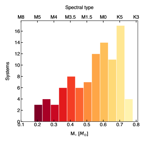
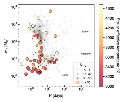
Figure 1: Sample of the study. Left: Distribution of the stellar spectral type (color coded by the effective temperature). Right: Period-mass diagram for all confirmed planets excluding those discovered by the imaging technique. Colored symbols correspond to the targets from our sample selected as explained in Sect. 2, where the color code indicates the effective temperature of the host star. The size of the colored dots informs on the number of RV measurements available for this work as indicated in the legend. The three horizontal lines show the masses of Jupiter, Neptune, and Earth for reference.

Our sample selection is based on the NASA Exoplanet Archive (NEA) planetary systems table (Akeson et al. 2013) in November 2023, which encompasses all the ”confirmed” planets to date. We applied the following criteria to select the sample.

First, the stellar effective temperature was set to be below 4650 K to focus the survey on low-mass stars. This corresponds with spectral types later than K4 V. Then, the system hosting up to two planets to avoid highly complex RV signals. This would reduce the number of free parameters and, consequently, the degree of degeneracy. Next, at least one of the planets must transit the star. This requirement relies on the methodology, as it exclusively applies to transiting planets. Finally, the transiting planets also have to be detected by radial velocities, since our method is based on the analysis of publicly available RVs.

A total of 88 systems fulfill these criteria. Seven of them were excluded for various reasons. According to the discovery papers, GJ~1132 and TOI~1266 require three Keplerians to reproduce the RV signal (Bonfils et al. 2018; Cloutier et al. 2024), indicating an additional planet candidate not listed in the NEA table. Kepler-16 is a binary star hosting a circumbinary planet that transits both stars (Triaud et al. 2022); hence, the detection method we used cannot be applied to this system (see Sect. 3). Kepler-91 is ascending the red giant branch and therefore is out of our regime of study (but see Lillo-Box et al. 2014, where the presence of a trojan for this system is studied). Also noteworthy are the cases of LHS~1815, TOI-2136, and Wendelstein-2, which have insufficient RV observations; therefore, the planet was undetectable and the candidate was only validated (Gan et al. 2020; Beard et al. 2022a; Obermeier et al. 2020). These cases highlight the need for establishing a protocol that standardizes the requirements for considering a planet as confirmed (Lillo-Box et al., in prep.), which would highly facilitate archival works.

Finally, we added K2-199, TOI-532, and TOI-1801 as these targets meet our constrains but at the time of writing are not yet included as detected by RV variations in the NEA. In summary, our final sample is composed of 84 systems hosting a total of 95 transiting planets. We note that our sample contains some targets previously analyzed in Lillo-Box et al. 2018a, b. However, we decided to preserve them for homogeneity. In some cases, new RV measurements are available, and we incorporated some changes in the analysis (e.g., we set the eccentricity to be below 0.1, and we fixed the orbital period and the mid-transit time to the photometric according to the prescription in Leleu et al. 2017; see Sect. 3).

All the RV datasets used in this work have been obtained from the literature. In Table B we summarize them, including the number of measurements (out of transit, see Sect. 3) and instruments, the time span, and the reference we retrieved the data from. The RV datasets used for all the targets can be found in Table 3. In Fig. 1, we illustrate the final sample. On the left, the stellar mass distribution showcases the covered spectral domain (spectral types are based on Cifuentes et al. 2020, valid for main-sequence low-mass stars). On the right panel, we show the period-mass diagram for all confirmed NEA exoplanets (excluding the ones detected by the imaging technique), where the color code indicates the stellar effective temperature and the sizes offer information on the number of RV measurements available for our analysis.

We conducted an examination of potential selection biases within our sample: (i) only 10 % of systems with confirmed planets fall within our target spectral domain (earlier than K4). To our knowledge, no works have shown co-orbital preference for any spectral type over another. However, Leleu et al. (2019) and Coleman et al. (2019) show that multiple planetary systems in resonant chains tend to retain the co-orbital configurations, two factors that could be more common around low-mass stars systems (e.g., Trappist-1); (ii) three systems (L 98-59, Demangeon et al. 2021; TOI-178, Leleu et al. 2021a; TOI-500, Serrano et al. 2022) lie outside our sample due to hosting more than two confirmed planets; this means our study comprises 97 % of low-mass star planetary systems and, therefore, no bias is anticipated from this constraint. We note that even if these stars are expected to host numerous planets (Kunimoto & Matthews 2020), they may remain undetectable with current instrumentation; (iii) like any statistical study focusing on transiting planets, our sample is biased towards large-radius planets in edge-on architectures. The former bias is compensated by the fact that low-mass stars host lighter and smaller planets and the signal of such planets in both techniques (RVs and transits) are also enhanced in this spectral domain. Specifically, 51 % of our observed planets are below a Neptune mass, 34 % fall between Neptune and Jupiter masses, and 15 % exceed the Jupiter mass. No effect is therefore expected in our study apart from the difficulty on studying the RV signals of the less massive planets. Regarding the edge-on orientation, as there are not obvious co-orbital transits in their light curves, our sample is biased to non-coplanar co-orbital configurations, or to small radii exotrojans; (iv) the spectral-type domain and the nature of the detection methods also contribute to the fact that the majority of planets in our sample have short periods (85% of them are below 10 days). Tidal interactions for those planets could have an impact preventing the long-term co-orbital stability (Correia et al. 2020) and this factor is even more critical around low-mass stars (Couturier et al. 2021). Therefore, for our sample we would expect to only find exotrojan evidence for the youngest systems or with longer orbital periods.

3 Methodology

A configuration with a single planet and a pair of co-orbitals can be identified using RV time series. Assuming a long time baseline and high cadence for the RV measurements, it is possible to detect the modulation in the main-planet signal as its trojan librates (see e.g., Leleu et al. 2015). Nonetheless, when the libration of the trojan is negligible as in the case of usual RV monitoring campaigns (spanning few months and with relatively sparse data), the key factor to reveal the presence of a co-orbital configuration is having information about the time of conjunction of the main planet (i.e., $T_{0}$). Even if the RV signal is compatible with a single planet scenario, the inferred transiting time from this technique would correspond with that of the centre of mass of the co-orbitals (Ford & Gaudi 2006). Therefore, if there is an imbalance in the masses of the Lagrangian regions, there would be a shift between the photometric and the RV inferred $T_{0}$. We note that this is the case as far as an asymmetry exists between the Lagrangian points L₄ and L₅: (i) a single trojan leading or trailing the main planet, (ii) two trojans each in its own tadpole (i.e., configuration in which the trojan librates around L₄ or L₅) region but unbalanced in mass, or (iii) a trojan in a horseshoe (i.e., the trojan travels from L₄ to L₅ going through L₃ as well) orbit but with a libration period larger than the observation time span. Conversely, this method would be ”blind” to equal mass trojans located in L₄ and L₅ regions. We note that all of these scenarios are equivalent when a swarm of asteroids replaces the compact body.

Leleu et al. (2017) generalized the RV equation as a function of time ($t$) for this method as follows:

$$\Delta v(t)=K\left[\left(\alpha-2c\right)\cos{nt}-\sin{nt}+c\cos{2nt}+d\sin{2nt}\right],$$ (1)

with $K$ as the RV semi-amplitude, and $n$ the mean orbital frequency. Parameters $c$ and $d$ depend on the orbital eccentricity ($e$) and the argument of periastron ($\omega$) as $c=e\cos{\omega}$, and $d=e\sin{\omega}$. The $\alpha$-parameter is the one that holds the trojan information. To the first order in eccentricity, it takes the form:

$$\alpha\,\simeq\,\rm{m_{t}}/\rm{m_{p}}\sin{\zeta},$$ (2)

where $\rm{m_{t}}/\rm{m_{p}}$ is the trojan-planet mass ratio, and $\zeta$ is the resonant angle that locates the trojan within the orbit (e.g., 60^∘/-60^∘ for L₄/ L₅). Thus, a significantly non-zero value of this parameter would suggest the presence of a massive trojan. As in Lillo-Box et al. (2018a), we follow the $\alpha$-test approach to search for trojans accompanying confirmed planets (i.e., transiting planets which mass has been measured through RVs). We note that Eq. 1 does not account for the Rossiter-McLaughlin (R-M) effect and for this reason, we removed the RV measurements taken during the transit.

The model and the amount of parameters that need to be explored depend on the number of detected planets ($N_{pla}$), transiting planets ($N_{tra}$), and instruments used to gather the measurements ($N_{ins}$). By construction, our sample is only composed of systems with one or two planets, and at least one of them must transit. The RV dataset of each transiting planet was modeled using Eq. 1, whose free parameters are the RV semi-amplitude ($K$), the orbital architecture ($c$ and $d$), and the $\alpha$ metric. The key to comparing the spectral and photometric mid-transit times relies on fixing the mean motion ($nt=2\pi\left[t\leavevmode\nobreak\ -\leavevmode\nobreak\ T_{0}\right]/P$), using the parameters inferred from the transits (collected in Table B). We note that for systems composed of two transiting planets, we searched for co-orbitals in both orbits simultaneously, fixing both periods and mid-transit times. Some of the literature values for the $T_{0}$ parameter were inferred in the corresponding works from a joint analysis considering also the RV data. Nonetheless, there is no conflict with this method since the $T_{0}$ parameter is mainly derived from the transiting signal as required (the RV dataset is typically not able to constrain it as precisely as the transits, on the order of minutes). Meanwhile, the RV signal of not-transiting planets was modeled with a classic Keplerian, whose parameters are $K$, $c$, $d$, $T_{0}$, and the orbital period, $P$. Finally, we added an offset and a jitter per instrument to account for instrumental dependencies and unaccounted systematics, respectively. Thus, we ended up with a total of $5N_{pla}\leavevmode\nobreak\ -\leavevmode\nobreak\ N_{tra}\leavevmode\nobreak\ +\leavevmode\nobreak\ 2N_{ins}$ parameters for the modeling.

If the activity of a star is affecting the RV time series, we included a Gaussian process (GP) to account for it. This decision was made when the rotational period ($P_{\rm rot}$) is present in the generalized Lomb-Scargle (GLS) periodogram of at least one spectral activity indicator such as the full width half maximum (FWHM) of the cross correlation function (CCF), the differential line width (dLW), or the H_α emission line, among others. In some occasions, the RV measurements are also correlated with the activity indicators showing that the same signal is present, and in the most obvious cases, the high RV scatter caused by the activity hinders the detection of the planetary signal. In all the cases, the GP was informed based on an activity proxy, which was chosen for being the indicator that most clearly shows $P_{\rm rot}$ (see Appendix A for the details on the particular cases). We implemented the GP using the george python package (Ambikasaran et al. 2015) opting for a quasi-periodic kernel (QP, e.g., Faria et al. 2016) of the form:

$$\Sigma_{ij}=\eta_{1}^{2}\,\rm{exp}\left[-\frac{(t_{i}-t_{j})^{2}}{2\eta_{2}^{2}}-\frac{2\rm{sin}^{2}\left(\frac{\pi(t_{i}-t_{j})}{\eta_{3}}\right)}{\eta_{4}^{2}}\right].$$ (3)

Hence, the GP implementation introduces increments into the number of parameters in $5\leavevmode\nobreak\ +\leavevmode\nobreak\ 2N_{ins}$. The proxy and the RV signal need an independent amplitude ($\eta_{1,\leavevmode\nobreak\ \rm{prx}}$ and $\eta_{1,\leavevmode\nobreak\ \rm{RV}}$), there is an aperiodic timescale ($\eta_{2}$), a correlation period ($\eta_{3}$), and a periodic scale ($\eta_{4}$). Additionally, the activity proxy requires a constant ($C$) and a jitter per instrument. We note that we only consider an amplitude $\eta_{1,\leavevmode\nobreak\ \rm{prx}}$ and $\eta_{1,\leavevmode\nobreak\ \rm{RV}}$ shared for all instruments. Therefore, it represents an average amplitude of the activity signal, which might not be ideal specially when the instruments cover different wavelength ranges.

To sample the posterior distribution of the model parameters we employ the Markov chain Monte Carlo (MCMC) affine invariant ensemble sampler emcee (Foreman-Mackey et al. 2013). We use five (ten when adding a GP) times the number of parameters for the walkers and between $6\times 10^{4}$ and $2\times 10^{5}$ steps, following a second run starting the new chains around the maximum a posteriori set of parameters and with half of the steps to speed up the convergence. The number of steps is adapted to ensure that the length of the chains is at least 50 times the autocorrelation time per parameter.

In Table 1 we show the priors adopted in the analysis. For most of the priors, we opt to use uniform distributions in order to be uninformative. In the case of the RV semi-amplitude ($K$), we choose the scatter of the RV ($RV_{\rm scatter}\,=\,RV_{\rm max}\,-\,RV_{\rm min}$) to be the upper limit of the uniform distribution. The selection of this prior has proven to be good enough as our posteriors on this parameter converge to values below half of the parameter space (i.e., RV_scatter/2). We choose equivalent priors for the amplitudes of the GP ($\eta_{\rm 1,prx}$ and $\eta_{\rm 1,RV}$). We did constrain $c$ and $d$ with a normal distribution for the planets with detected secondary eclipses by computing their values as Eqs. 33 and 34 from Winn (2010) and changing their sign to transform into the planet frame (see Table 4). These are the most reliable candidates since $\alpha$ is degenerated to some extent with the orbital architecture ($e$), being the secondary transit the only means to disentangle them. When no secondary eclipse is available, we need to work under the assumption of low-eccentricity orbits ($e\,<\,0.1$) to be able to apply our methodology since Eq. 1 is only valid for eccentricities below this value. Hence, it is important to note that our results are subjected to this scenario. When the orbital period of the planets (either transiting or not) are below 10 d, we do an additional test setting them to circular orbits ($e\,=\,0$, as based on the tidal circularization criterion, for example, Jackson et al. 2008). In the case of systems where one of the planets does not transit, we used normal distributions for the Priors of $P$ and $T_{0}$ using the data from the bibliography tabulated in Table B. The priors for the GP hyperparameters are normal distributions based on literature posteriors if a QP GP has already been implemented for that particular system, or are those shown in Table 1 otherwise.

Table 1: Prior distributions. The subscripts identify parameters only applicable for transiting ($tra$), and not transiting ($ntr$) planets, and ($occ$) are for the values inferred from occultations.

Parameter	Prior	Units
$K$	$\mathcal{U}\left(0,\leavevmode\nobreak\ \rm{RV_{scatter}}\right)$	m s-1
$c$	$\mathcal{U}\left(-1,\leavevmode\nobreak\ 1\right)$ or $\mathcal{G}_{t}\left(c_{occ},\leavevmode\nobreak\ \Delta c_{occ}\right)$
$d$	$\mathcal{U}\left(-1,\leavevmode\nobreak\ 1\right)$ or $\mathcal{G}_{t}\left(d_{occ},\leavevmode\nobreak\ \Delta d_{occ}\right)$
$e_{tra}$	$\mathcal{U}\left(0,\leavevmode\nobreak\ 0.1\right)$
$P_{ntr}$	$\mathcal{G}_{t}\left(P,\leavevmode\nobreak\ \Delta P\right)$	d
$T_{0,\leavevmode\nobreak\ ntr}$	$\mathcal{G}_{t}\left(T_{0},\leavevmode\nobreak\ \Delta T_{0}\right)$	d
$\alpha$	$\mathcal{U}\left(-1,\leavevmode\nobreak\ 1\right)$
jitter	$\mathcal{U}\left(0,\leavevmode\nobreak\ \rm{RV_{scatter}}/4\right)$	m s-1
offset	$\mathcal{U}\left(\rm{RV_{\rm{min}}},\leavevmode\nobreak\ \rm{RV_{\rm{max}}}\right)$	m s-1
	GP hyperparameters
$C$	$\mathcal{U}\left(\rm{Proxy_{min},\leavevmode\nobreak\ Proxy_{max}}\right)$	Proxy units
jitterprx	$\mathcal{U}\left(0,\rm{\leavevmode\nobreak\ Proxy_{scatter}/4}\right)$	Proxy units
$\eta_{1,\leavevmode\nobreak\ \rm{prx}}$	$\mathcal{U}\left(0,\leavevmode\nobreak\ \rm{Proxy_{scatter}}\right)$	Proxy units
$\eta_{1,\leavevmode\nobreak\ \rm{RV}}$	$\mathcal{U}\left(0,\leavevmode\nobreak\ \rm{RV_{scatter}}\right)$	m s-1
$\eta_{2}$	$\mathcal{U}\left(2P_{rot},\leavevmode\nobreak\ 1\,000\right)$	d
$\eta_{3}$	$\mathcal{G}_{t}\left(P_{rot},\leavevmode\nobreak\ \Delta P_{rot}\right)$	d
$\eta_{4}$	$\mathcal{U}\left(0,\leavevmode\nobreak\ 5\right)$

4 Results

There are 95 transiting planets from the 84 systems for which we can inspect their $\alpha$ searching for co-orbital signs. We test up to four models per system: the slightly eccentric orbit model (where the eccentricity is either below 0.1 or constrained by the secondary eclipse), the circular orbit model (if $P<10$ d), and those two models but including a GP if needed ($P_{\rm rot}$ signal present in a spectral indicator). We selected the GP model as the best one (when available) and we decided among the circular and eccentric models by means of the Bayes factor ($\ln\cal{Z}$), computed with the bayev code (Díaz et al. 2016). Remarkably, for all of the cases the circular model (simpler) is favored over the eccentric scenario, with $\ln\cal{Z}$ $>3.5$.

We classified the sample into four groups based on the inferred $\alpha$. The most relevant are the ”strong candidates” (SC) and the ”null detections” (ND) groups since they provide conclusive results. The SC are the planets with an $\alpha$ value different from zero within a 99.7 % confidence interval ( $|\alpha|$ /$\sigma_{\alpha}\geq 3$), therefore being co-orbital detections by the $\alpha$-test. On the other hand, ND are planets with null $\alpha$ values as far as the uncertainty is below 15 % ($\sigma_{\alpha}<0.15$), being observationally very expensive to better constrain the presence of an hypothetical co-orbital and, therefore, we rule them out as candidates. In between, we distinguish the ”weak candidates” (WC), and the ”inconclusive candidates” (INC). For both of them, there is a large uncertainty in terms of their $\alpha$ values that would be required to gather more (or more precise) data until reaching conclusive results. Nonetheless, for the WC, the $\alpha$ differs from zero within 1-$\sigma$ to 3-$\sigma$, hinting at the presence of trojans as promising targets that should continue to be monitored. In Table 2, there is a summary for this classification criterion. We note that the sum of the members is 94 since one of the targets (GJ 3090 b) is rejected for being out of the methodology domain (see Appendix A for more details).

Table 2: Target classification.

$\alpha^{a}$	Criterion	Group	Members
$\neq$ 0	$|\alpha|/\sigma_{\alpha}>3$	Strong candidate	1
	$1<|\alpha|/\sigma_{\alpha}<3$	Weak candidate	25
= 0	$\sigma_{\alpha}>0.15$	Inconclusive	21
	$\sigma_{\alpha}<0.15$	Null detection	10
	$\Delta\phi>0.15$ or	Sparsely sampled	37
	N${}_{RVs}<15$

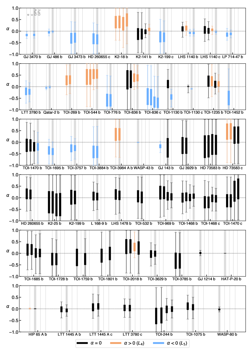
Figure 6: Inferred $\alpha$ parameter for the transiting planets ordered by groups as in Table B. The analysis of each planet is divided in four different models (dotted vertical lines) corresponding, from left to right, with the slightly eccentric orbit (e), the circular orbit when the period of the planet is under 10 d (c), and both of these adding a GP if required (GPe and GPc). The model used for the co-orbital mass estimation in Sect.5.1 is indicated with a vertical grey region. The null value is indicated with an horizontal dashed line. Color-code informs on the result of $\alpha$ within 1-$\sigma$ as indicated in the legend. Errorbars show the 68.3% (wide bar) and 99.7% (narrow bar) confidence intervals (1 and 3-$\sigma$).

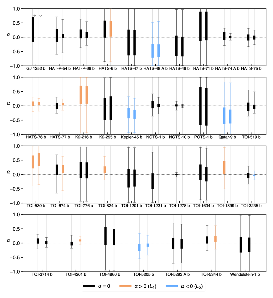
Figure 7: Inferred $\alpha$ parameter for the targets sparsely sampled. See details in the caption of Fig. 6.

A large number of transiting planets in the sample (37, being the 40 %) have a poor coverage in the orbital phase space. The criterion we adopted to tag a system as ”sparsely sampled” (SS) is that each orbital phase bin of 0.15 contains less than one measurement (i.e., $\Delta\phi>0.15$, being $\Delta\phi$ the orbital phase difference between consecutive data points), or the total number of data points is below 15 (i.e., N${}_{RVs}<15$). We included these targets in the analysis for completeness and also because they are relevant targets with respect to expanding the sample in the near future. Nonetheless, we did not classify them in the groups mentioned above and we do not consider them for the discussion. The resulting $\alpha$ for all the tested models can be found in Table B and are displayed in Fig. 6 for the grouped targets, and Fig. 7 for the SS.

Only one planet stands out as SC: GJ 3470 b. This is a hot Neptune of around 14 $M_{\oplus}$ in a 3.3-days orbit that has been intensively explored. There is no evidence for the existence of a second planet orbiting the M-dwarf, including no significant TTVs (below 500 s, Awiphan et al. 2016). The outcome of the analysis corresponds with a co-orbital detection at a 3-$\sigma$ level ($\alpha=-0.16\leavevmode\nobreak\ \pm\leavevmode\nobreak\ 0.05$). GJ 3470 b is a very strong candidates not only by its significance, but also because it is not degenerated with the orbital architecture since the secondary eclipse of this planet has been observed with Spitzer. For more information on the analysis, we refer to Appendix A.

Remarkably, both transiting planets orbiting TOI-1130 have not null $\alpha$ values with a higher significance ($\sim$ 4- and 12-$\sigma$) than GJ 3470. Nonetheless, we downgrade them to WCs, since Korth et al. (2023) reported strong TTVs in both planets (more than 2 hours of amplitude for planet b) by using TESS and ground-based photometry. As Leleu et al. (2017) warn, planets with coupled orbital periods in 2:1 MMR (as in the case of TOI-1130, with 4.1 and 8.4 days) can induce false positives due to their possible TTVs. Nonetheless, the time span of the RV dataset we use (62 days) covers around 15 orbits of the inner planet, which should mitigate the TTV impact in the inferred $\alpha$. For this reason, we either rule out this target as a candidate. Other systems near 2:1 MMR are present in the sample: HD 260655 (with periods of 2.8 and 5.7 days), K2-199 (3.2 and 7.4 days), TOI-776 (8.2 and 15.7 days), and TOI-836 (3.8 and 8.6 days). All of these targets have at least one not null $\alpha$, yet TOI-836 c is the only planet that exhibits TTVs in the order of 20 minutes (Luque et al. 2021, 2022; Hawthorn et al. 2023). We recall, as mentioned above (Sect. 2), that resonant chains are expected to help preserving the co-orbital stability.

The cases of GJ 143 b, and HIP 65 A b are also noteworthy. The former planet orbits a presumably active star as its rotational period appears in the activity indicators. Nonetheless, when including a GP the uncertainty in $\alpha$ is greatly increased in almost a factor of five, taking this target from the WC group to the INC. For HIP 65 A b, the result hardly depends on the eccentricity being a WC for the slightly eccentric model and ND for the circular. Since this planet has a grazing transit (b $\sim$ 1 according with Nielsen et al. 2020), breaking the degeneracy through the eclipse might not be possible.

It is interesting to note that HAT-P-20 b and WASP-43 b have an extraordinary low uncertainty, namely: 0.2 and 0.5 % of the $\alpha$ parameter space. Both of them are favoured due to the fact that they are hot Jupiters that induce a big RV semi amplitude into their stars ($\sim$ 1240 and 555 m s^-1), by the determination of the eccentricity by the occultation and also by the high quality of their observations (using HARPS and ESPRESSO spectrographs). In the case of WASP 43 b, the majority of the measurements were taken around the transit, which is also likely to favour an accurate mid-transit time being obtained through the RVs, as an advantage for our methodology. This was also found for WASP-80 b (see Appendix A).

5 Discussion

5.1 Co-orbital mass

In order to estimate the trojan mass we use Eq. 2 by fixing $\zeta$ = $\pm 60^{\circ}$. These resonant angles correspond to tadpole orbits in which the co-orbitals librate around L₄ or L₅, the most common configurations based on numerical simulations (e.g., Leleu et al. 2019). We take the percentiles at the 95.45% confidence interval (2.3 and 97.7) of the $\alpha$ posterior distribution inferred for the best model per system (see Sect. 4, and specified in Table B) to compute the upper limit on the trojan mass. We tabulate those masses in Table B. For the only SC in our sample (GJ 3470 b), we obtain the predicted posterior distribution of the trojan mass in L₅ by taking the whole distribution of $\alpha$, resulting in m_t = 2.6 $\pm$ 0.7 $M_{\oplus}$.

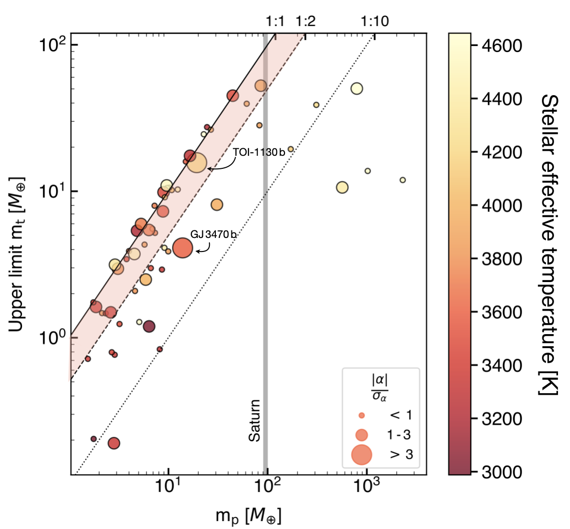
Figure 2: Upper limit of the trojan mass versus the mass of the confirmed planet. Black lines indicate equal mass ratios (solid line) along with the 1:2 (dashed) and 1:10 relations (dotted). The vertical grey solid line indicates the mass of Saturn. The light orange region corresponds to trojan masses higher than theoretically expected (between 1:1 and 1:2). The size of the symbols informs about the significance of the co-orbital candidate as shown in the legend. Color code represents the stellar effective temperature as shown in the color bar.

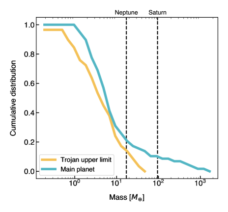
Figure 3: Occurrence rate of trojans and mass distribution of the main planets.

Figure 2 graphs the maximum of the co-orbital mass upper limit (between L₄ and L₅) as a function of the planetary mass. In this diagram, we find that for 34 of the planets (59 %), the upper limit of the hypothetical trojans is above half of the mass of the main planet (within the light orange region). We would expect this area to be empty based on theoretical studies (Pierens & Raymond 2014); indeed, most of those targets correspond to the WC and INC groups, underscoring the fact that our current datasets do not constraint the co-orbital presence. On the other hand, only ten targets (17 %) have the mass ratio $\rm{m_{t}}/\rm{m_{p}}$ restricted to be below the 20 %. Interestingly, six of those are the only planets in our sample with planetary masses above Saturn ($\sim 100\,M_{\oplus}$). From this observational result based on the available time series and the $\alpha$-test method, we can infer two conclusions: (i) currently, for planets less massive than Saturn we cannot restrict the presence of trojans; and (ii) there is no observational evidence for the presence of trojans more massive than Saturn around low-mass stars. Notably, some of the less massive planets (e.g., GJ 486 b, LHS 1140 c, and TOI-244 b) have their co-orbital companions restricted in more than the 50 %. The reason is that a more exhaustive RV monitoring with outstanding precision was needed for their detection, which shows that it is currently feasible to carry out dedicated searches to efficiently restrict the uncertainties in the $\alpha$ parameter.

In Fig. 3, we show the cumulative lower limit occurrence rate of trojans as a function of their upper mass limits, compared with the distribution of the confirmed main planets. As already discussed, there are no Saturn-mass trojans expected accompanying the giant planets that orbit low-mass stars, which represent 15 % of our sample. Less than the 18 % of the planets are expected to be accompanied by Neptune-mass trojans, and roughly 80 % can have trojans less massive than the Earth. Comparing with the confirmed population of Neptunes (20 %) and with planets less massive than the Earth (100 %, since such planets remain undetectable to date), we notice again that current RV datasets are unable to give strong constraints to the presence of co-orbitals and, therefore, on the occurrence rate.

5.2 Search for Lagrangian point transits

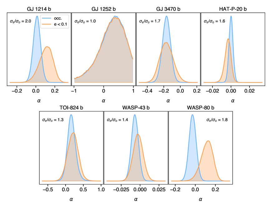
Figure 4: Comparison of the $\alpha$ posterior distribution when using normal priors for the orbital architecture informed from the occultation (blue) and when using uniform priors with e ¡ 0.1 (orange). The improvement in the precision as the ratio of their $\sigma$ is shown in the upper corner of each chart.

Under the assumption of (near) circular orbits and (near) coplanarity of the main planet and the potential co-orbital companion, if the main planet transits its host star from our line of sight, the co-orbital could also do so. Hence, for the cases where we find some hints for the presence of co-orbital bodies (WC sample), it is worth checking the available space-based time series photometry around the Lagrangian regions, seeking for a dimming induced by these (still weak) candidates. It is however relevant to mention that while having near-circular orbits is a requisite to apply our $\alpha$-test, coplanarity is neither required not necessary to keep the stability of a co-orbital pair (e.g., Leleu et al. 2017). Consequently, non-detections within this exercise only constrain the parameter space for the existence of the trojan corresponding to the near-coplanar case, while larger mutual inclinations are still possible.

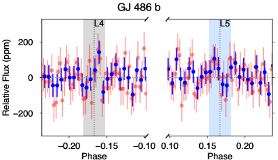
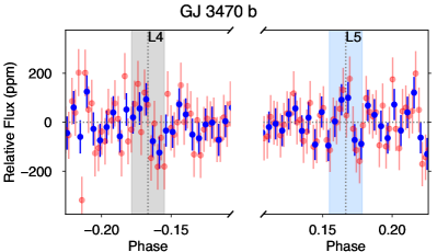
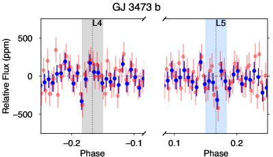
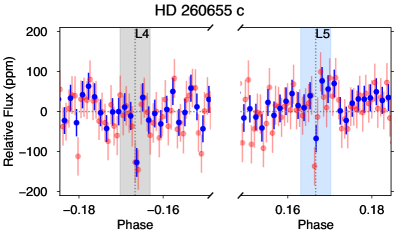
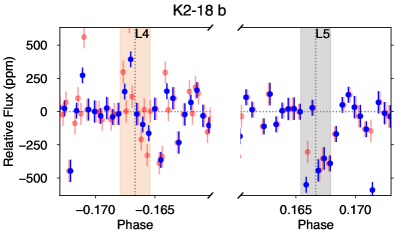
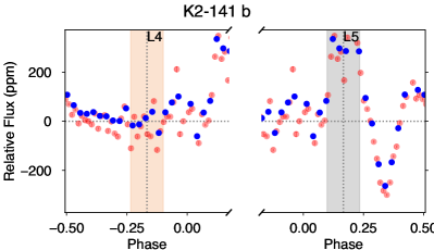
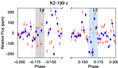
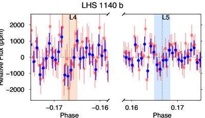
Figure 9: Phase-folded light curves (from the TESS mission, except for K2-18 b, K2-141 b, and K2-199 c where we used the K2 data) around the $L_{4}$ and $L_{5}$ regions for the weak candidate (WC) sample. The phase-folded light curves are binned with a bin size corresponding to 10% (red symbols) and 20% (blue symbols) of the main-planet transit duration. The Lagrangian point phase of conjunction is marked by a dotted vertical line and the shaded region indicates the duration of the main-planet transit. We highlight in color (blue for $L_{5}$ and orange for $L_{4}$) the region where our model indicates the potential location of the co-orbital, while in gray the opposite region. Cases where both regions are colored indicate systems where some of the models (circular versus eccentric) showed candidates at either Lagrangian point.

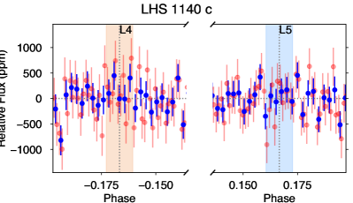
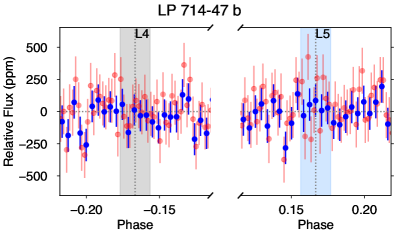
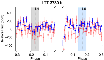
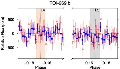
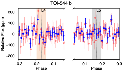
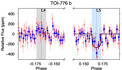
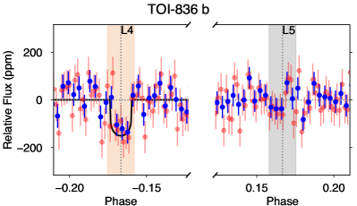
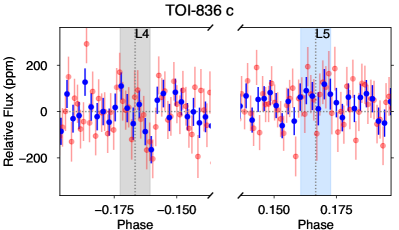
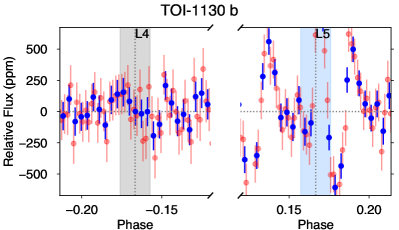
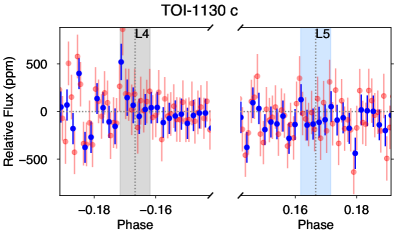
Figure 9: Continuation.

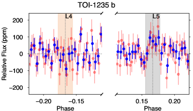
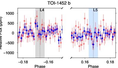
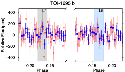
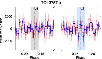
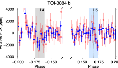
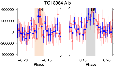
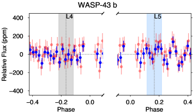
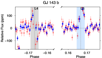
Figure 9: Continuation.

Our main light curve source is the Transiting Exoplanets Satellite Survey (TESS, Ricker et al. 2014), but when available, we also retrieved the K2 data (Borucki et al. 2010; Howell et al. 2014). We use the lightkurve (Lightkurve Collaboration et al. 2018) package to retrieve the processed detrended light curves from these missions. For TESS, we use the SPOC pipeline (Jenkins et al. 2016) with a 2-min cadence. For K2, we use the K2 pipeline with a 30-min cadence. For each of the planets in the WC list, we retrieved the light curve from all available sectors (TESS) or campaigns (K2). We then performed a detrending using wōtan (Hippke et al. 2019). To this end, all transits from any planet in the system are masked. The detrended and normalized light curves are then phase-folded with the planet ephemeris. The zoomed-in light curves around the Lagrangian points L₄ and L₅ for each planet are presented in Fig. 9, with bin sizes corresponding to 10% (red symbols) and 20% (blue symbols) of the planet’s transit duration. On each panel, we mark in color (orange for L₄ and blue for L₅) the Lagrangian point where our $\alpha$-test has yielded the (weak) candidate. In most cases, the light curves around these regimes show a flat behaviour, with no detectable transits.

In some cases (specially in the K2 data) the light curves are very noisy, potentially due to stellar activity not appropriately removed with our detrending process. However, in some few cases, the light curves seem to show dimmings compatible with the duration and location expected for a co-orbital planet. In particular, this is the case for LHS 1140 b, which shows very shallow dimmings at both L₄ and L₅, although still compatible with the noise. Other two interesting cases are TOI-776 b (L₅) and TOI-836 b (L₄). They both show relatively clear dimmings at their corresponding Lagrangian points where the $\alpha$-test locates the co-orbital candidates. The dimmings would correspond to objects of around 1 $\mathrm{R}_{\oplus}$. The estimated masses for the trojan candidates given the inferred $\alpha$ values are $2.8\pm 1.6$ $\mathrm{M}_{\oplus}$ (TOI-776 ${\rm L_{5}\,b}$) and $1.9\pm 0.9$ $\mathrm{M}_{\oplus}$ (TOI-836 ${\rm L_{4}\,b}$). The estimated planet radius for such masses using the empirical relations from Chen & Kipping (2017) are $1.44^{+0.78}_{-0.42}$ $\mathrm{R}_{\oplus}$ and $1.18^{+0.49}_{-0.25}$ $\mathrm{R}_{\oplus}$, respectively. Interestingly, these values match the detected dimmings. Further observations on these system will be critical to provide additional insights towards the confirmation of these candidates. Meanwhile, there are no detectable dimmings for GJ 3470 b. This means that there is no transiting counterpart for the strong trojan candidate with radius larger than $\sim$1 $\mathrm{R}_{\oplus}$.

5.3 Occultations

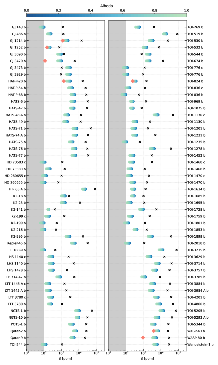
Figure 5: Depths of the transit (black cross), predicted occultation (color-coded as function of the albedo), and true occultation if measured (salmon diamond) per planet. Dashed line is at 100 ppm, considering the grey area as the undetectable regime by current instrumentation.

Throughout this study, we have emphasized the critical importance of detecting occultations to reliably constrain the planetary eccentricities. This methodology stands as the sole means to resolve the degeneracy between eccentricity and $\alpha$. Only seven planets within our sample have had their secondary transits measured to our knowledge. In order to visualize the improvement, in Fig. 4, we compare the posterior distribution of their $\alpha$ with the one obtained if no occultation were to be observed (assuming e ¡ 0.1). For all the cases (except for GJ 1252 which is part of the SS targets), the precision in the inferred $\alpha$ is increased, being a factor two for GJ 1214. The magitude is also shifted in some of the cases, being a false candidate in GJ 1214 and WASP 80, when no occultation is measured. In this section, we focus on assessing the feasibility of detecting more occultations among our target planets.

When the planet is eclipsed by the host star, the received flux is reduced the quantity corresponding to that of the emitted by the planet. Its emission is compound by the thermal radiation and the reflected starlight. The former is only not negligible as compared with the starlight when observing at long wavelengths. Hence, infrared instruments such as Spitzer/IRAC were used to maximize the planet emission, which translates to a higher flux dimming. To estimate the eclipse depth we consider both the planet and the star emit as blackbodies, that in the mid-infrared can be approximated by Rayleigh-Jeans taking the form (e.g., Winn 2010; Encrenaz 2014):

$$\delta_{occ}=0.01\left(\frac{R_{p}/R_{J}}{R_{\star}/R_{\odot}}\right)^{2}\frac{T_{eq}}{T_{\star}},$$ (4)

where $R_{p}$ and $R_{\star}$ are the planet and stellar radius in Jovian and solar units respectively, and $T_{eq}/T_{\star}$ is the planet equilibrium and stellar temperature ratio. With the same assumption, we can also estimate $T_{eq}$ as:

$$T_{eq}=279\,(1-a)^{0.25}\left(\frac{T_{\star}/K}{5770}\right)\left(\frac{R_{star}/R_{\odot}}{D/AU}\right)^{0.5},$$ (5)

where $a$ is the geometric albedo and $D$ is the planet-star distance in au. At shorter wavelengths, the reflected emission from the star might be detectable and it also depends on $a$, $D$, and $R_{p}$. Nonetheless, the occultation depth is maximum at the mid-infrared where this component can be ignored. In Fig. 5, we show the measured transit depths and the estimated occultation depths as a function of the albedo for all the confirmed planets in the sample. For the few targets with this quantity measured, it is also represented here. We have found that they are compatible with the theoretical approximation (except for GJ 3470 b and WASP-80 b), but all of them are overestimated. This is probably because empirically the wavelenght used is around 4.5 $\mu$m but the thermal emission would be increased at higher wavelenghts (e.g., using JWST/MIRI, which covers up to 28 $\mu$m).

Since this study is focused on the low-mass stellar domain, our sample enhances the occultation depth (i.e., $\delta_{occ}\propto R_{\star}^{-2}$). For this reason, most of the eclipses are expected to be detectable with current instrumentation ($\delta_{occ}>100$ ppm). We particularly encourage monitoring the secondary eclipse of the weak candidates resulted from this work, since it would translate in a reduction of the $\alpha$ uncertainty.

6 Conclusions

We have carried out an extensive search for exotrojans around low-mass stars with spectral types later than K4 V. We analyzed publicly available RV time series aiming at identifying mass imbalances within the orbital paths of their confirmed planets. We found a strong candidate for a trojan of $2.6\pm 0.7M_{\oplus}$ in the L₅ point of the hot Neptune GJ 3470 b. Additionally, for other two targets which show a weak evidence for the presence of co-orbitals, we also spot a dimming in the predicted Lagrangian point (L₅ for TOI-776 b, and L₄ for TOI-836 b) in their TESS light curves.

The results of the analysis show that the current data permit constraints to be placed on the presence of co-orbitals accompanying planets more massive than Saturn. Interestingly, less massive planets ($<3M_{\oplus}$, such as GJ 486, LHS 1140, or TOI-244), which have been confirmed using the most precise instruments and a wealth of measurements, highlight the potential for significantly reducing the upper limits of co-orbital masses when using more demanding observational strategies (e.g., strategies devoted to the improvement in the precision of the planetary masses). This would lead to a more refined constraint on the presence of trojans and, consequently, would enhance our ability to infer their occurrence rate.

The sample was divided into different groups based on the resulting $\alpha$ parameter. There is particular interest in the targets classified as WC and SS to continue the RV observations. Among the WC, those targets with fewer (or less precise) RV measurements are particularly promising for further investigation using this technique. These planets exhibit a high degree of uncertainty in $\alpha$, yet their 63% confidence interval exclusively considers the possibility of a co-orbital scenario (non-null values). Some of these targets include K2-199, TOI-776, TOI-1452, TOI-3757, TOI-3884, and TOI-3984 A. Additionally, all targets classified as SS are highly desirable for continued observation via RV measurements. Special attention is warranted for GJ 1252 and TOI-824, since it is expected to derivate credible $\alpha$ values, given their well-known eccentricity as their secondary transit is measured.

Conversely, for some other targets within the WC group, it is not worthwhile to continue the RV monitoring as the observational cost overweigh the potential for improvements. These candidates need to be studied in more detail through other techniques, such as photometrically inspecting the Lagrangian regions, combining the photometrical observations with dynamical models (e.g., Lillo-Box et al. 2018b), and even directly imaging with future missions such as LIFE (Quanz et al. 2022). Priority should be given to the search for the occultation of the main planet in order to break the degeneracy of the trojan presence with the orbital architecture. Based on the estimation of the occultation depth (Sect. 5.3), the most promising targets (with depths above $10^{3}$ ppm) among the WC to measure the eclipse in infrared light are: GJ 3473 b, K2-18 b, LP 714-47 b, Qatar 2 b, TOI-544 b, TOI-3757 b, TOI-3884 b, and TOI-3984 b.

It is important to note that a null detection in the context of our methodology does not definitively rule out the presence of co-orbital companions, yet it does significantly limit it. Adhering to the tadpole configurations assumption (Sect. 5.1), their masses are already tightly constrained, and further narrowing these limits is not expected. Conversely, it is plausible that co-orbitals could escape our detection approach. For instance, horseshoe configurations could have $\alpha$ values oscillating to zero at each instance that could result in a false negative provided the libration timescale is shorter than the RV time span. Such scenarios may be detectable through alternative detection methods meriting their exploration in future studies (e.g., RV modulations due to the trojan libration, e.g., Leleu et al. 2015).

This work serves to advocate for the RV monitoring of the stars devoted to the search for co-orbitals. It also provides guidelines that can aid in this objective, and a list of the most relevant targets. As demonstrated in previous works of this series (Lillo-Box et al. 2018a, b, increasing the number of measurements and their precision is crucial. In the present work, WASP-43 b and WASP-80 b suggest that not only an appropriate (i.e., homogeneous) coverage of the orbital phase is needed, but increasing the monitoring on phases close to the transit could benefit the determination of the spectroscopic mid-transit time, which directly translates into a lower uncertainty of the $\alpha$ parameter.

Appendix A Radial velocity analysis per system

In this section, we give the details of the RV analysis for the individual targets.

A.1 Strong candidate

GJ 3470

Located in the hot-Neptune desert, GJ 3470 b has been object of many studies trying to bring light to the rare population to which it belongs. As a result, we account with multiple high-precision RV measurements. The RV analysis requires a linear trend probably caused by an undetected stellar companion, for which we inferred a slope of ($-0.0022\leavevmode\nobreak\ \pm\leavevmode\nobreak\ 0.0011)\,{\rm m}\,{\rm s}^{-1}\,{\rm d}^{-1}$. The secondary eclipse of this planet has been observed, allowing us to set normal priors on the $c$ and $d$ parameters that were derived in this work using the eclipse published in Benneke et al. (2019), and obtaining compatible results with those from Kosiarek et al. (2019) (see Table 4). Even there is no clear correlation between the RV measurements and the activity indicators, we included a GP informed with the $S_{\rm HK}$ index as it shows a peak in its GLS at $P_{\rm rot}\,=\,21.5\leavevmode\nobreak\ \pm\leavevmode\nobreak\ 0.5$ d. The resulting $\alpha$ places this target as a SC with a 3-$\sigma$ significance.

A.2 Weak candidates

GJ 486

This single-planet target has an $\alpha$ parameter different from 0 in 1-$\sigma$ in both slightly eccentric ($e\leavevmode\nobreak\ <\leavevmode\nobreak\ 0.1$) and circular orbit scenarios. We do not include a GP to the analysis since, according with Caballero et al. (2022), none of the periodograms of the activity indicators (e.g., H_α, Ca II, or Na I) show any significant peak that could suggest the star is active.

GJ 3473

Our RV analysis for the confirmed planet GJ 3473 b resulted in an $\alpha$ parameter different from 0 within 1-$\sigma$ for both tested models, the slightly eccentric ($\alpha=-0.30^{+0.23}_{-0.24}$) and the circular orbit ($\alpha=-0.28^{+0.21}_{-0.22}$). Based on the $H_{\alpha}$ emission line, this target is considered inactive (Jeffers et al. 2018).

HD 260655

Both planets in this system transit the star with short periods, lying in a close 2:1 MMR ($P_{b}\,=\,2.8\,$d, and $P_{c}\,=\,5.7\,$d). However, these rocky worlds do not show significant TTVs according with Luque et al. (2022). Based on the values obtained for the $H_{\alpha}$ emission and $R^{\prime}_{\rm HK}$, this star is thought to be inactive with a rotation period of around $\sim$30 d. Our analysis found that, contrary to the inner planet, the outer one has an $\alpha$ parameter different from zero within 1-$\sigma$ ($\alpha=-0.32^{+0.22}_{-0.25}$) indicating that the mass of its potential co-orbital companion could be higher than the one for the inner planet. This result is hold when considering circular orbits. As warned in Leleu et al. (2017) (and discussed in Sect. 4), planets in 2:1 MMR are susceptible to mimic co-orbitals in the $\alpha$-test method. Nonetheless, as no TTVs are detected and the RV time span is huge (24 years) in comparison with the orbital periods, a false positive caused by the planetary configuration is not expected. Detailed searches to constrain their presence is needed, such as photometrically inspect the Lagrangian regions in the search for dimmings (see Sect. 5.2).

K2-18

With an orbital period of 32.9 d, K2-18 b is a Super-Earth in the habitable zone (HZ) of an M-dwarf. We use the RVs extracted with the recent line-by-line (LBL) method (Artigau et al. 2022) published in Radica et al. (2022). They identified 14 outliers in CARMENES and three in the HARPS datasets, resulting in a total time series of 147 measurements after discarding those data points. This system has been claimed to host an additional not-transiting planet in a 9.2 d orbit confidently detected with the LBL RVs after rejecting a particular night (December 25, 2016). We include a GP informed with the dLW, indicator showing a peak in the GLS at the estimated stellar rotational period ($\sim 39\,$d). The analysis suggests the presence of a co-orbital for K2-18 b with an $\alpha\leavevmode\nobreak\ =\leavevmode\nobreak\ 0.48^{+0.29}_{-0.28}$.

K2-141

K2-141 b is an ultra-short period planet orbiting at 0.28 d. There is an additional validated transiting planet with a period of 7.7 d that is not detected with the RV dataset. Therefore, we carried out the analysis only considering planet b. The RV dataset shows a considerably big scatter. Besides, all the GLS of the activity indicators present a peak at $P_{rot}\leavevmode\nobreak\ =\leavevmode\nobreak\ 14\,$d, so we add a GP by using the FWHM as proxy. Our analysis was compatible with a configuration with an low-mass co-orbital within $L_{4}$ as $\alpha\leavevmode\nobreak\ =\leavevmode\nobreak\ 0.07\pm 0.07$.

K2-199

The K2 mission detected two transiting planets orbiting around K2-199, at 3.2 and 7.4 d orbital periods. Activity tracers suggest the star is moderately active. Nonetheless, Akana Murphy et al. (2021) opted for a model not including a GP since the spot behaviour of the star changed between the campaigns and therefore they did not achieve the convergence of the hyperparameters. Not accounting for the activity either, we found that the outer planet has a similar $\alpha$ for both eccentric ($\alpha=-0.25^{+0.23}_{-0.24}$) and circular ($\alpha=-0.26^{+0.20}_{-0.21}$) models.

LHS 1140

Two transiting planets orbit this M-dwarf star with periods of 3.8 (LHS 1140 c) and 24.7 d (LHS 1140 b, lying within the HZ). LHS 1140 has already been target of co-orbital search through the $\alpha$-test in Lillo-Box et al. (2020). There, it is discarded the presence of a co-orbital for LHS 1140 b more massive than 1 M_⊕, but found a co-orbital candidate for LHS 1140 c. Here, we re-analyze the system using the same observations but with a different RV extraction (using the LBL method, Cadieux et al. 2024) that is expected to improve the uncertainty on the inferred $\alpha$ parameter, and with some changes in the analysis as mentioned in Sect. 2. An additional external planet was proposed in Lillo-Box et al. (2020) based on the RV signal, but it was not supported by the new LBL dataset (Cadieux et al. 2024). Therefore, we consider LHS 1140 as a two-planets system. A GP is clearly needed in the model, with a rotational period of around 131 days appearing in the FWHM. Both transiting planets arise to be WC, with $\alpha_{b}=-0.11^{+0.07}_{-0.02}$, and $\alpha_{c}=-0.04\leavevmode\nobreak\ \pm\leavevmode\nobreak\ 0.02$, assuming circular orbits.

LP 714-47

LP 714-47 b is a planet located in the hot-Neptune desert ($P\,=\,4.1\,$d, $R\,=\,4.7\,R_{\oplus}$). The scientific interest of this target motivated its RV follow-up using multiple instruments, such as ESPRESSO and CARMENES. In the original publication, Dreizler et al. 2020 found that the rotational period of the star is present in the GLS of the RVs ($\sim$ 33 d). Though, according with the periodogram of the activity tracers presented in their work, that signal is not obvious in any of them. For this reason, and since such indicators are not available and our residuals do not show much scatter, we do not include a GP in our model.

LTT 3780

A pair of TESS-candidate planets were confirmed using spectroscopic data around LTT 3780 with orbital periods of 0.8 d and 12.3 d. The star is known to be rather inactive, as indicated by the $R^{\prime}_{\rm HK}$ value of $-5.59$ (Cloutier et al. 2020a). Additionally, no modulation appears in the photometric data. Given that no strong activity impact is expected, we chose not to include a GP in this test.

Qatar-2

Qatar-2 b is a hot Jupiter in a 1.3 d orbit around a K-dwarf star. Its strong photometric variations reveal the active nature of the star with a rotational period of $\sim$ 18.5 d, which corresponds with a gyrochronological young age of around 1.4 Gyr (Esposito et al. 2017; Močnik et al. 2017). From the RV dataset in hand, only HARPS-N data have activity tracers available (nine out of the 80 out of transit data points). Such few FWHM measurements are not enough to account for the activity contribution on the signal and thus we do not include a GP to our analysis. We obtain an $\alpha$ different from zero in 1-$\sigma$ ($\alpha=-0.02\leavevmode\nobreak\ \pm\leavevmode\nobreak\ 0.02$, in the circular case).

TOI-269

The sub-Neptune (2.8 R_⊕, 8.8 M_⊙) orbiting this M2-dwarf star with a 3.7 d period has been reported to be highly eccentric ($\sim$ 0.43). This solution is obtained by Cointepas et al. (2021) when fitting together transits and RV datasets. Based on the mature stage of the system ($\sim$2-4 Gyr) and the short orbital period of the planet, it would be expected to have circularized the orbit. To explain the puzzling result, they invoked the inward migration of the planet through a planet-planet interaction as an hypothesis. As explained in Sect. 3, the eccentricity is highly degenerated with $\alpha$, and thus it was not surprising to obtain an $\alpha$ different from zero ($\alpha=0.29^{+0.20}_{-0.18}$ for a circular orbit) in our analysis. Since the occultation of this planet has not been measured, the eccentricity is not constrained and the co-orbital scenario is also a plausible alternative to the uncommon high-eccentricity. As the authors explain in their work, the host star is though to be quiet and probably has a long rotation period ($\sim$ 69 d). As in the original work, we did include a linear trend to the analysis with a resulting slope significantly different from zero (0.021 $\pm$ 0.008$\,\rm{m}\,\rm{s}^{-1}\,\rm{d}^{-1}$).

TOI-544

The star hosts a small planet discovered by TESS in a short period of 1.5 days. The RV dataset is composed of HARPS and HARPS-N campaigns taken over nearly three years, which enabled the detection of a non-transiting Neptune-mass planet at a 50.1 day period. The S-index shows a very clear peak at 19 days, which we interpret as the rotational period. When we include a GP the scatter of the RV residuals are greatly reduced, yet it is still larger than in Osborne et al. (2024b) since they use a two-dimensional GP. The result of the analysis is compatible with the existence of a co-orbital companion within the $L_{4}$ region ($\alpha=0.57^{+0.19}_{-0.22}$).

TOI-776

Three signals are required in order to model the RVs of this system: two Keplerians to account for the two transiting planets, and a sinusoidal function describing the activity. The sinusoidal function has the periodicity of the rotation of the star (34.4 days), and an amplitude of 2.7 m s^-1. It was shown by Luque et al. (2021) that this model explains well the observations and it is not necessary to appeal to a GP. Both planets are mini Neptunes with orbital periods of P_b = 8.3 d and P_c = 15.7 d. The signal for the outer planet is inadequately sampled based on the criterion adopted at the beginning of this section (i.e., there is a phase gap greater than 15% for P_c), and hence, we only put attention on the $\alpha$ parameter inferred for the inner planet. The inferred aforementioned parameter is different from zero ($\alpha=-0.62^{+0.29}_{-0.24}$ for the circular case) and thus it could point to a mass imbalance towards the $L_{5}$ region. We warn that, even the period of planet b is well sampled according with our criterion, there exists a scarcity of data around the orbital phase $\phi$ = 0.

TOI-836

Two transiting planets were detected using two TESS Sectors (11 and 38): a super-Earth (P_b = 3.8 d), and a mini-Neptune (P_c = 8.6 d). The K V star is very active being imperative the use of a GP to detect the planetary signals in the HARPS RV dataset. We use the FWHM, which informs on the stellar rotational period being around 22 days. Based on the discovery paper (Hawthorn et al. 2023), the existence of TTVs with an amplitude of $\sim$20  min for TOI-836 c may suggests the existence of an outer planet not yet detected either by RVs or transits. As discussed in Sect. 4, TTVs can induce false positive co-orbitals since the $T_{0}$ varies. However, the TTVs amplitude is very low in comparison with the RV time-span so we do not expect a big impact on our analysis. The results locate both targets as interesting candidates with not-null $\alpha$ at a 2.4 and 2.8-$\sigma$ level for the inner and outer planets respectively. Furthermore, the light curve inspection comes as a suprise, with an interesting dimming in the L₄ region of TOI-836 b that is compatible with the location and the radius inferred from its $\alpha$ value (see Sect. 5.2).

TOI-1130

This system is composed of a K-dwarf orbited by an inner Neptune-sized planet (TOI-1130 b) and an outer hot Jupiter (TOI-1130 c). TESS light curves show that the time of mid-transit of both planets varies at each orbit, with an amplitude of 2.5 h for TOI-1130 b, and 0.25 h for TOI-1130 c. This is cause by the resonant configuration in 2:1 MMR (P_b = 4.1 d, P_c = 8.4 d). The HARPS RV time series present a linear trend with a slope of $\sim 0.5\,{\rm m}\,{\rm s}^{-1}\,{\rm d}^{-1}$ likely induced by an undetected outer companion. Both planets are clearly detected with these RVs, and the result of our analysis return not-null $\alpha$ values for both planets with very high significance ($\alpha_{b}=-0.44^{+0.12}_{-0.11}$, and $\alpha_{c}=-0.09\pm 0.01$). However, there is a high probability that these results are affected by the known TTVs, even the time span of the RV dataset is higher than the TTVs period. For this reason, we do not consider them as SC but as WC (see Sect. 4).

TOI-1235

This M0.5 dwarf is orbited by the transiting planet TOI-1235 b, which is located in the radius gap ($\sim$1.7 $R_{\oplus}$, $\sim$6-7 $M_{\oplus}$) in a 3.44 days orbit (Bluhm et al. 2020; Cloutier et al. 2020b). The RV data set comprises CARMENES, HARPS, and HIRES measurements. Its GLS shows an additional signal around 21 days, which is also present in the dLW GLS. Therefore, we include a GP informed with this activity indicator and considering a normal prior for $\eta_{3}$ of $P_{\rm rot}=20.93\pm 0.6$ d. The result barely places the target as a WC, with a not-null $\alpha$ just at 1-$\sigma$ level ($\alpha=0.12^{+0.12}_{0.11}$).

TOI-1452

TOI-1452 b is a super-Earth in a 11.1-days orbital period first detected by its transit with TESS, and later confirmed with SPIRou and IRD RVs (Cadieux et al. 2022). For the analysis, we opt for not including the IRD data since they are few measurements in comparison with the SPIRou not including additional information in our case but increasing in one the number of free parameters. For most of the SPIRou nights around three to four measurements were taken. For this reason, we use the night-binned measurement to reduce the measurement uncertainty. As detailed in the discovery article, the host star does not show any obvious rotational period, so we consider it as a quiet star. As the orbital period is higher than 10 days, we do not test the circular model (see Sect. 3). The inferred $\alpha$ suggest the presence of a co-orbital companion ($-0.51^{+0.33}_{-0.30}$).

TOI-1695

A wealth of SPIRou and HARPS-N measurements enabled confirming the planetary nature of the transiting super-Earth TOI-1695 b identified by TESS ($P=3.13$ d, $\sim 2.0R_{\oplus}$, $\sim 6M_{\oplus}$, Kiefer et al. 2023, Cherubim et al. 2023). The photometric estimation of the rotational period of the star ($P_{\rm rot}\sim 48$ d) corresponds with an inactive early M-dwarf, which is consistent with the spectroscopic indices showing very weak indicators of activity. The circular model of our analysis is compatible with the presence of a co-orbital within 2.5-$\sigma$ ($\alpha=-0.40^{+0.14}_{-0.16}$).

TOI-3757

TOI-3757 b is one of the few gas giants orbiting an M-dwarf ($P=3.4$ d, around 12 $R_{\oplus}$, and $\sim 85M_{\oplus}$, Kanodia et al. 2022). The available RV dataset is composed of HPF and NEID measurements. We do not include a GP since it does not show hints of activity. The slightly eccentric and the circular model provide compatible results, with an $\alpha_{\rm c}=-0.25\pm 0.13$. We note that this target labeled as a WC is a good opportunity to keep its RV monitoring in order to improve the data set (higher precision and more measurements).

TOI-3884

The TESS photometry of this M4-dwarf shows the transit of a super-Neptune of 6.4 $R_{\oplus}$ in a 4.5 days orbit affected by star-spots in several orbits. An upper limit to its mass has been confirmed with a dataset of HPF (Libby-Roberts et al. 2023a) and a couple of measurements from ESPRESSO (Almenara et al. 2022a). Interestingly, even the star is known to be active, a GP does not improve the RV analysis as tested by Libby-Roberts et al. (2023a). In both our eccentric ($\alpha=-0.42^{+0.27}_{-0.28}$) and circular ($\alpha=-0.41^{+0.25}_{-0.27}$) models, this target is a WC with a 1-$\sigma$ significance.

TOI-3984 A

The RV analysis for this M4-dwarf star is based on a dataset of 41 NEID and HPF measurements. The star is orbited by a transiting giant of 4.4 day period (0.14 $M_{J}$, 0.71 $R_{J}$), and is the primary of a multiple system with a wide binary. With the available data, this target results a WC at a 1.3-$\sigma$ level ($\alpha=0.34^{+0.27}_{-0.26}$).

WASP-43

The case of the hot Jupiter WASP-43 b ($\sim 2M_{J}$ with a period of 0.8 days) around a K7V star has been widely studied since its discovery (Hellier et al. 2011). Despite what would be expected, considering its location and mass, this planet does not experience orbital decay (Hoyer et al. 2016). For our analysis, we opted for using only the HARPS and ESPRESSO data available in the ESO Archive with Program IDs 0102.C-0820, 60.A-9128, 089.C-0151, 096.C-0331, and 0104.C-0849, since there are a high quantity of them and are of great quality. We note that the observations were mainly taken around the transit as a cause of the original scientific goal. Such observational strategy probably favours obtaining a more accurate measurement of the mid-transit time through RVs, which favours our methodology. Moreover, the occultation of the planet has been observed breaking the $\alpha$-eccentricity degeneracy (Blecic et al. 2014). The host star is though to be very active based on the high value of the log($R^{\prime}_{\rm HK}$), which could be enhanced by the close Jupiter and its youth (Esposito et al. 2017). However, the rotational period of the star (around 16 d according with Hellier et al. (2011)) is not present in the GLS of the FWHM, therefore we do not include a GP. The result of the analysis suggest the presence of a co-orbital up to 11 $M_{\oplus}$ within L₅ ($\alpha=-0.007\pm 0.005$).

A.3 Inconclusive

GJ 143

Apart from the confirmed planet (GJ 143 b), this star hosts an additional inner transiting candidate at 7.8 d (GJ 143 c). However, the available RVs are not sensitive enough to detect that candidate (Dragomir et al. 2019). Consequently, we only include GJ 143 b in our model and a linear trend to account for a long-term. Among the GLS periodogram of the available activity indicators for the HARPS data subset, we find a peak at 37.1 d (close but not overlapping with the planet orbital period, $P_{b}\,=\,35.6\,$d) in the FWHM of the cross correlation function (CCF), which is compatible with the rotational period proposed in Dragomir et al. (2019). Therefore, we add a GP informed with the FWHM as activity proxy. The uncertainty in the $\alpha$ parameter is greatly increased when including the GP in contrast with the not-null $\alpha$ value (2-$\sigma$) inferred for the model without the GP. Therefore, although it falls within the group of INC targets, it is convenient to study this planet by alternative methods such as transits (see Sect. 5.2).

GJ 3929

The RV dataset shows the presence of the confirmed transiting hot Earth-sized GJ 3929 b ($P_{b}\,=\,2.6\,$d), and a candidate not transiting sub-Neptune ($P_{c}\,=\,15.0\,$d) around the M3.5V star (Kemmer et al. 2022; Beard et al. 2022b). This star is thought to be inactive based on different indicators (e.g., H$\alpha$, flat light curve). Even in the discovery article they include a GP, based on the quiet behavior and since the $\alpha$-test do not show hints for the presence of a Trojan candidate, we opt for not including a GP.

HD 73583

This system is composed of two transiting mini-Neptunes discovered by TESS (TOI-560) which are close to a 3:1 MMR ($P_{b}\,=\,6.4\,$d, and $P_{c}\,=\,18.9\,$d). This is a clear case of a young ($\sim 500\,$Myr) active star affecting the RVs. As in Barragán et al. (2022), we used the $S_{\rm HK}$ time-series as activity indicator to feed the GP, which has a peak in the GLS periodogram at $P\leavevmode\nobreak\ \sim\leavevmode\nobreak\$12 d, as the periodicity found in the TESS light curves. The posterior distributions found are compatible with those from their work. We note that they use a more sophisticated method using a multidimensional GP by adding the derivate of the QP kernel as a component of the RV model, resulting in cleaner residuals of the model. None of the two planets resulted in an $\alpha$ parameter different from zero.

K2-25

Young planetary system ($730\,\pm\,50\,$Myr, Mann et al. 2016) hosting a Neptune-sized planet at an orbital period of 3.5 d. As expected due to its youth, our preliminary RV analysis show large residuals and thus we decide to test a GP based on the dLW as activity tracer. We set a normal prior for $\eta_{3}$ as the rotational period estimated by Stefansson et al. (2020), $P_{rot}\,=\,(1.878\,\pm\,0.005\,)$d. The result did not support the presence of a co-orbital. Nonetheless, we note that obtaining more precise RVs is currently possible for this target and it would likely improve this test. Thus, this analysis should be revised in the future.

L 168-9

This M1V dwarf hosts a transiting super-Earth discovered by TESS in a close orbit (1.4 days). Looking at the GLS of the activity indicators, it is not evident whether there is an effect of stellar activity in the RVs: HARPS indices show a forest of peaks near $P_{rot}$ and its harmonics ($\sim$20 days based on Astudillo-Defru et al. 2020), meanwhile for PFS, there are no peaks related. Thus, we opt for not including a GP. Our analysis resulted in an $\alpha$ compatible with no co-orbital mass.

LHS 1478

TESS detected a hot super-Earth in a 1.9 days orbital period that was later confirmed through CARMENES RVs (Soto et al. 2021). In our analysis, we decide to not include the IRD data since they are sparse and do not add significant information to the $\alpha$-test. This M-dwarf star is inactive based on the $H_{\alpha}$ emission and therefore, we do not include any GP. We do not find hints for the presence of co-orbitals, but improvement in the analysis could be made by acquiring more RV measurements.

TOI-532

This M-dwarf hosts a super Neptune ($\sim$ 62 M_⊕) orbiting with a 2.3 day period. The flat light curve detected by TESS suggests that this star is probably inactive (Kanodia et al. 2021). There is no suspect so far that the planet could harbor a co-orbital based on the RVs dataset. Although we note that this target have not been extensively monitored and the uncertainty in $\alpha$ is potentially narrowable.

TOI-969

The late K-dwarf star TOI-969 is transited by a close mini-Neptune in a 1.8 day period (TOI-969 b, located at the lower boundary of the hot-Neptune desert). The combination of 94 RV measurements with HARPS, PFS and CORALIE revealed the presence of a second companion in the system, the candidate TOI-969 c ($\sim$ 11 $M_{J}$). We do not include the CAROLIE dataset in our analysis since the associated uncertainties are too high to detect the transiting planet (tens of m/s). As in the original article (Lillo-Box et al. 2023), we model the RV long-term with a Keplerian of $P_{c}=1700\pm 290$ d, which is the signal of the outer candidate. To account for the activity, we include a GP informed with the $\log{R^{\prime}_{\rm HK}}$ computed for HARPS. The GLS of such indicator has its strongest peak at $\sim$24 d, with aliases at 12 and 8 d. The same signal appears in the WASP photometry according with Lillo-Box et al. (2023), which confirms that it corresponds with the rotational period of the K-dwarf. The result does not favor the presence of a co-orbital companion ($\alpha=0.03^{+0.16}_{-0.14}$).

TOI-1468

Two transiting low-mass planets were detected and confirmed around this M3 V star using TESS photometry, and a dataset of 81 CARMENES and MAROON-X RVs (Chaturvedi et al. 2022). The inner planet orbits the star with a 1.9 d period (TOI-1468 b), while the outer orbits every 15.5 d. The H$\alpha$ index is a good proxy for the rotational period as its GLS shows a clear signal close to 41 d. The preferred model of our analysis (including the GP and with the inner planet in a circular orbit) is compatible with no co-orbitals ($\alpha_{b}=0.12^{+0.17}_{-0.10}$, and $\alpha_{c}=0.01^{+0.11}_{-0.21}$).

TOI-1470

The RV monitoring of the M1.5 V TOI-1470 with CARMENES confirmed the TESS transiting sub-Neptune TOI-1470 b ($P_{b}=2.5$ d), as well as other transiting planet in a 18.1 d orbit first reported by González-Álvarez et al. (2023), TOI-1470 c. We use H$\alpha$ as spectral activity indicator of the rotational period ($\sim$ 29 d) to perform a GP analysis. The results are compatible with no co-orbitals but with wide uncertainties ($\alpha_{b}=-0.18^{+0.14}_{-0.19}$, $\alpha_{c}=0.44^{+0.39}_{-0.51}$).

TOI-1685

The CARMENES (Bluhm et al. 2021) and IRD (Hirano et al. 2021) RV time series allowed us to confirm the planetary nature of the transiting super-Earth TOI-1685 b, which orbits its M3 V star with an ultra-short period of just 0.7 d. Bluhm et al. (2021) reported a moderated evidence for the presence of a second not-transiting planet in the system (TOI-1685 c) with an orbital period of 9.0 d based on the CARMENES dataset. In our IRD + CARMENES combined analysis, we find an increase in the evidence for its presence, with a logarithm of the Bayes Factor of 10 when comparing the two-planets model with the single transiting planet. We also include a GP informed with the CARMENES dLW indicator, with a normal prior in the rotational period of ($18.7\pm 0.7$) d. The result is affected of high uncertainty in the inferred $\alpha$ with the available dataset: $\alpha=0.18^{+0.27}_{-0.16}$.

TOI-1728

With an orbital period of 3.5 d, the super-Neptune TOI-1728 b transits an old and inactive M0-dwarf star (Kanodia et al. 2020). We include a linear trend to our RV model to account for a long-term with an inferred slope of ($-0.14\pm 0.17$) $\rm{m}\,\rm{s}^{-1}\,\rm{d}^{-1}$. The results of the $\alpha$-test (compatible with no trojans with $\alpha=-0.22^{+0.23}_{-0.29}$) are here limited due to the relatively low-precision of the uncertainties associated with its HPF RV measurements, which are in the order of tens of m/s.

TOI-1759

The sub-Neptune TOI-1759 b was first detected through three transits from different TESS sectors. Later, independent works using CARMENES (Espinoza et al. 2022) and SPIRou (Martioli et al. 2022) RVs confirmed the planet orbiting the M0-dwarf star with a 18.8 d period. Our analysis is only based on the CARMENES dataset since it has a better presicion compared with the SPIRou measurements, and we checked that the latter do not improve the inferred $\alpha$. We introduce a GP informed with the dLW, which shows the rotational periodicity at $\sim 36$ d and is consistent with the inferred from the SPIRou dataset. The inferred $\alpha$ is $-0.23^{+0.24}_{-0.27}$.

TOI-1801

TOI-1801 b was identified by TESS photometry and confirmed by CARMENES and HIRES RVs. It is a transiting young mini-Neptune orbiting with a 10.6 d period a M dwarf younger than 1 Gyr (Mallorquín et al. 2023). We include to the MCMC analysis a GP informed with the H$\alpha$ time series (peak at P${}_{\rm rot}\sim 16$ d in its GLS). The high scatter in the RVs even after the GP correction results in high uncertainties for the inferred $\alpha$ ($-0.05^{+0.33}_{-0.25}$).

TOI-2018

The metal poor K-dwarf TOI-2018 is transited by a mini-Neptune with an orbital period of 7.4 d. We use the available HIRES measurements correcting them from the stellar activity informing a GP through the $S_{\rm HK}$ index ($P_{\rm rot}\sim 21$ d). A vague constraint can be made for the presence of co-orbitals given the high uncertainty of the result ($\alpha=0.19^{+0.33}_{-0.25}$).

TOI-3785

The M2-dwarf star TOI-3785 hosts a low-density transiting Neptune of 4.7 d orbital period. The parent star is thought to be inactive (Powers et al. 2023) thus no GP is introduced even there is a high scatter in the RV measurements. Note that six of the RV data points have a bigger uncertainty since they were taken with a shorter exposure time. The quality of the data do not allow the $\alpha$ parameter to be constrained, resulting in a non-informative $\alpha=-0.33\pm 0.33$.

A.4 Null detections

GJ 1214

This is a extensively studied planetary system in the literature. Only one planet has been detected (the sub-Neptune GJ 1214 b) and the star is known to be inactive. The recent detection of its secondary eclipse (Kempton et al. 2023) confirmed that the planet is almost in a circular orbit. Our analysis was very well constrained not requiring a GP and with informative priors on $c$, and $d$. For this reason and in light of the result, this target is perfectly compatible with an scenario with no Trojan, with a very low upper limit to the Trojan mass (0.8 $M_{\oplus}$, see Sect. 5.1).

HAT-P-20

HAT-P-20 has been thoroughly studied since its discovery (Bakos et al. 2011). Multitude of transits and RV measurements have been gathered, including observations of the R-M (Esposito et al. 2017), the absence of significant TTVs have been confirmed (e.g., Sun et al. 2017; Lillo-Box et al. 2018b), and the secondary eclipse has been observed twice in two Spitzer bands (Deming et al. 2015) confirming a slightly eccentric orbit. As first noticed by Knutson et al. (2014), the RVs have a linear trend which is potentially caused by the visual companion of HAT-P-20. Thanks to these previous efforts, $\alpha$ is estimated with an small uncertainty being able to reject this object as a co-orbital candidate based on the $\alpha$-test ($\alpha=0.000\pm 0.002$). The result is compatible with the one already presented in Lillo-Box et al. 2018b.

HIP 65 A

This star (TOI-129) hosts a hot-Jupiter of $\sim 3\,M_{J}$ in a $0.98\,$d orbital period. Its light curve reveals that the star is active, showing modulations with a periodicity of $\sim 13\,$d. As argued by Nielsen et al. (2020), the available RV dataset is unaffected by the activity since the impact is of the order of $\sim 10\,\rm{m}\,\rm{s}^{-1}$, which is comparable to the RV uncertainty of the FEROS measurements, and 2-3 times smaller than those from CORALIE and CHIRON. Additionally, none of the available activity indicators show any relevant periodicity. The result places this target as a co-orbital candidate. Interestingly, the result differs when assuming a circular orbit, where the $\alpha$ drops to a value compatible with zero. This is a good example to show the importance of breaking the $\alpha$-eccentricity degeneracy through the secondary eclipse. In Sect. 5 we predict the expected occultation depths for all the targets, being HIP 65 A one of the most promising ($\delta\leavevmode\nobreak\ >\leavevmode\nobreak\ 10^{4}\,$ppm). Our solution where $\alpha$ differs from zero corresponds with a slightly eccentric orbit that would imply that the occultation would happen around $18\,$min before of the expected time, at an orbital phase of $0.487\,\pm\,0.003$. Nonetheless, since this planet has a grazing transit, this exercise might not be possible.

LTT 1445 A

LTT 1445 A is the primary star of a hierarchical triple system. It is orbited by the transiting planet LTT 1445 A b, which has an orbital period of 5.4 d. Winters et al. 2022 found the RV signal of a second planetary body in a closest orbit, LTT 1445 A c with 3.1 d. The result of the analysis reject this target as a candidate for both planets ($\alpha_{b}$ = -0.07 $\pm$ 0.08, and $\alpha_{c}=0.10^{+14}_{-0.13}$, for the circular case).

TOI-244

The bright M2V dwarf hosts a transiting super-Earth in a 7.4 days orbital period with a characteristic low density. The spectral activity indicators (FWHM, $H_{\alpha}$ and S-index) clearly show the stellar rotational period in their periodograms at $P_{rot}\sim 56$ days, indicating that this is an active star. As in the discovery article (Castro-González et al. 2023), we include a GP to mitigate this effect from the RVs by using the FWHM as proxy. Since after subtracting the stellar contribution the HARPS data still showing a big scatter, we opt for only including the ESPRESSO dataset to our analysis. As a result of the wealth of high-precision RV time-series, we can constrain the presence of co-orbitals to be below 0.8 $M_{\oplus}$ ($\alpha=-0.01\pm 0.12$).

TOI-1075

The Super-Earth TOI-1075 b orbits its M0-type parent star with an ultra-short period of just 0.6 d. The star does not show any sign of activity. The RV dataset requires a linear trend with an slope that we infer to be of 0.14 $\rm{m}\,\rm{s}^{-1}\,\rm{d}^{-1}$, which might be attributed to an outer planetary-mass companion. The PSF RV time-series do not show any shift in the mid-transit time of TOI-1075 b ($\alpha=0.07\pm 0.13$).

TOI-3629

TESS discovered a Jupiter orbiting close to this M1-dwarf star with a 3.9 day period. The subsequent gathering of 28 RV measurements with NEID and HPF confirmed this candidate and enables rejecting the possibility of having a co-orbital object more massive than 28.2 $M_{\oplus}$. Even this target is classified according with Table 2 as a Null Detection ($\alpha=-0.01\pm 0.13$), it would be desirable to decrease the Trojan upper limit by extending the sample and even increasing the precision of the RVs ($<10$ m s^-1).

WASP-80

This interesting confirmed transiting planet, halfway between warm Neptunes and hot Jupiters (171 $M_{\oplus}$, P = 3 days), was already studied through the $\alpha$-test in Lillo-Box et al. (2018a). As its occultation was already known in this previous article, the target has a low uncertainty with an $\alpha=0.038^{+0.083}_{-0.085}$. Six years later, the RV sample has been increased from 47 to 73 measurements, mainly grouped around the transit since its atmosphere has been studied with HARPS. Thanks to that observational effort, we now get $\alpha=-0.03\pm 0.04$, reducing the uncertainty in a factor two and therefore, greatly decreasing the upper limit of the Trojan mass (from 44.7 $M_{\oplus}$ to 8.7 $M_{\oplus}$ in L₄, and from 28.5 $M_{\oplus}$ to 19.4 $M_{\oplus}$ in L₅). This example shows that gathering numerous RVs with orbital phases close to 0 might favor the search for co-orbitals by this method as the mid-transit time could be better constrained.

A.5 Sparsely sampled

GJ 1252

GJ 1252 b stands out as a Super-Earth of particular interest for characterization due to its notably short orbital period ($P\,=\,0.5\,$d), low stellar activity, and the observation of a day-side eclipse. Even though, the RVs for GJ 1252 b have been poorly monitored, with a limited time span of less than 11 days. Consequently, continued tracking of this target is imperative to accumulate more comprehensive data and derive a conclusive $\alpha$ parameter.

TOI-824

The K4-dwarf star is orbited every 1.4 days by one of the few known hot Neptunes (with a radius of 2.9 R_⊕, and a mass around 18.5 M_⊕). The exotic of its nature and its elevated surface temperature makes it a very interesting target for atmospheric characterization. Therefore, its occultation has been measured with Spitzer which has constrained the planet to be in a circular orbit. This under-sampled target is perfect to gather additional data to better constrain the $\alpha$ parameter and thus its possibility of harboring a co-orbital companion.

A.6 Rejected case

GJ 3090

This star hosts a transiting mini-Neptune on a 2.9 d orbit. Almenara et al. (2022b) reported the RV signal of a candidate second planet with an orbital period of 12.7 d. Their RV analysis resulted in a solution where both planets are in very eccentric orbits ($e_{b}\,\sim\,0.2$, and $e_{c}\,\sim\,0.3$). Our priors do not allow for eccentric orbits for GJ 3090 b since Eq. 1 is only valid when e ¡ 0.1. Despite the degeneracy between $e$ and $\alpha$, our solution do not favor the co-orbital scenario. The model found is quite noisy, which translates into a big uncertainty for the $\alpha$ parameter, probably caused by the presence of stellar activity. Indeed, the GLS periodogram of the RVs show some signal at the rotational period ($\sim\,18\,$d) and its first harmonic ($\sim\,9\,$d). As argued in Almenara et al. (2022b), the quasi-periodic kernel in the GP does not converge, but adding a cosine component (QPC kernel) it improves. We repeat the same procedure using the QPC informed with the $H_{\alpha}$ indicator. Nonetheless, we still found problems in the convergence since GJ 3090 b is restricted to not very eccentric orbits. This target is therefore outside the validity domain of the $\alpha$-test. For this reason, we do not include this target in the sample for the discussion.

Appendix B Additional tables

[x]lcccccccc Summary of the archival radial velocities and parameters adopted in this work.

System Planet N_RVs N${}_{\rm ins}^{a}$ Timespan [d] Transits P [d] $T_{0}$ – 2 450 000 [d] Ref.^b RV / param.

Continuation.

System Planet N_RVs N${}_{\rm ins}^{a}$ Timespan [d] Transits P [d] $T_{0}$ – 2 450 000 [d] Ref.^b RV / param.

GJ 143 b 283 4 5942.8 Yes 35.61253${}^{+0.00060}_{-0.00062}$ 8385.92502${}^{+0.00054}_{-0.00055}$ Dra19
GJ 486 b 243 7 1967.1 Yes 1.467119${}^{+0.000031}_{-0.000030}$ 8931.15935 $\pm$ 0.00042 Cab22 / Tri21
GJ 1214 b 163 2 3734.8 Yes 1.58040433 $\pm$ 0.00000013 5701.413328${}^{+0.000066}_{-0.000059}$ Clo21a
GJ 1252 b 20 1 10.9 Yes 0.51824160 $\pm$ 0.00000069 8668.09748 $\pm$ 0.00032 Shp20 / Luq22b
GJ 3090 b 55 1 326.0 Yes 2.853136${}^{+0.000064}_{-0.00038}$ 8370.41849 $\pm$ 0.00034 Alm22a
GJ 3470 b 193 5 4709.1 Yes 3.3366496${}^{+0.0000039}_{-0.0000033}$ 5983.70421$\pm$0.00010 Lil18, Ste22 / Awi16
GJ 3473 b 148 3 358.2 Yes 1.1980035${}^{+0.0000018}_{-0.0000019}$ 8492.20408${}^{+0.00043}_{-0.00042}$ Kem20
c No 15.509 $\pm$ 0.033 8575.6 $\pm$ 2.2
GJ 3929 b 97 2 528.6 Yes 2.616235 $\pm$ 0.000005 8956.39620 $\pm$  0.00050 Bea22, Kem22 / Bea22
c No 15.040 $\pm$ 0.030 9070.9 $\pm$ 2.0
HAT-P-20 b 57 4 2857.8 Yes 2.8753172 $\pm$ 0.0000003 5917.64480461 $\pm$ 0.00000010 Bak11, Knu14, Esp17, Lil18 / Sun17
HAT-P-54 b 17 2 410.0 Yes 3.799847 $\pm$ 0.000014 6299.3037 $\pm$ 0.00024 Bak15
HAT-P-68 b 13 3 1100.0 Yes 2.29840551 $\pm$ 0.00000052 6614.20355 $\pm$ 0.00014 Lin21
HATS-6 b 15 3 259.2 Yes 3.3252725 $\pm$ 0.0000021 6643.74058 $\pm$ 0.000084 Har15
HATS-47 b 12 1 151.7 Yes 3.9228038 $\pm$ 0.0000022 7365.35804 $\pm$ 0.00029 Har20
HATS-48 A b 11 1 125.8 Yes 3.1316666 $\pm$ 0.0000037 7100.55022 $\pm$ 0.00045 Har20
HATS-49 b 8 1 536.3 Yes 4.1480467 $\pm$ 0.0000037 7105.1648 $\pm$ 0.00054 Har20
HATS-71 b 7 1 744.0 Yes 3.7955202 $\pm$ 0.0000010 7858.80134 $\pm$ 0.00023 Bak20
HATS-74 A b 5 1 5.0 Yes 1.73185606 $\pm$ 0.00000055 8392.02654 $\pm$ 0.00024 Jor22
HATS-75 b 5 1 6.1 Yes 2.7886556 $\pm$ 0.0000011 8611.05487 $\pm$ 0.00027 Jor22
HATS-76 b 3 1 6.1 Yes 1.9416423 $\pm$ 0.0000014 8424.55556 $\pm$ 0.00053 Jor22
HATS-77 b 5 1 25.9 Yes 3.0876262 $\pm$ 0.0000016 9136.69378 $\pm$ 0.00020 Jor22
HD 73583 b 87 1 334.1 Yes 6.398042${}^{+0.0000067}_{-0.0000062}$ 8517.69013${}^{+0.00056}_{-0.00059}$ Tes21, Bar22 / Odd23
c Yes 18.87974${}^{+0.00086}_{-0.00074}$ 9232.1682${}^{+0.0019}_{-0.0024}$ Tes21, Bar22 / Bar22
HD 260655 b 180 2 8794.5 Yes 2.76953 $\pm$ 0.000030 9497.91020 $\pm$ 0.00030 Luq22a
c Yes 5.70588 $\pm$ 0.000070 9490.36460 $\pm$ 0.00040
HIP 65 A b 90 3 491.9 Yes 0.9809734 $\pm$ 0.0000031 8326.102581$\pm$ 0.000050 Nie20, Par21 / Nie20
K2-18 b 146 2 1189.9 Yes 32.9396 $\pm$ 0.0004 7264.39140 $\pm$ 0.00070 Rad22
c No 9.207${}^{+0.007}_{-0.006}$ 7267.581${}^{+0.480}_{-0.467}$
K2-25 b 31 1 427.8 Yes 3.484545${}^{+0.000042}_{-0.000043}$ 7062.57958${}^{+0.00054}_{-0.00056}$ Ste20 / Tha20
K2-141 b 74 2 1500.9 Yes 0.2803244 $\pm$ 0.0000015 7744.07160 $\pm$ 0.00022 Bar18, Mal18, Bon23 / Bon23
c Yes 7.7485 $\pm$ 0.00022 7751.1546 $\pm$ 0.001
K2-199 b 45 1 1071.0 Yes 3.2253993 $\pm$ 0.0000024 7218.73733${}^{+0.00051}_{-0.00055}$ Aka21
c Yes 7.3744897 $\pm$ 0.0000037 7222.93034 $\pm$ 0.00035 Aka21
K2-216 b 26 4 488.7 Yes 2.1748 $\pm$ 0.000050 7394.04170 $\pm$ 0.00090 Per18
K2-295 b 6 1 108.7 Yes 4.024867 $\pm$ 0.000015 7395.4140500 $\pm$ 0.0000010 Smi19
Kepler-45 b 14 1 92.7 Yes 2.455239 $\pm$ 0.0000040 5003.822000 $\pm$ 0.000036 Joh12
L 168-9 b 123 2 106.0 Yes 1.4015 $\pm$ 0.00018 8340.04781${}^{+0.00088}_{-0.00122}$ Ast20
LHS 1140 b 254 3 1470.9 Yes 24.737230 $\pm$ 0.000020 8399.93000 $\pm$ +0.00030 Men19, Cad24 / Cad24
c Yes 3.777940 $\pm$ 0.000020 8389.29390 $\pm$ +0.00020 Men19, Cad24 / Cad24
LHS 1478 b 57 1 261.3 Yes 1.9495378${}^{+0.0000040}_{-0.0000041}$ 8786.75425 $\pm$ 0.00042 Sot21
LP 714-47 b 81 5 314.5 Yes 4.052037 $\pm$ 0.0000040 9196.11490 ${}^{+0.00031}_{-0.00030}$ Dre20
LTT 1445 A b 135 5 643.4 Yes 5.3587657${}^{+0.0000043}_{-0.0000042}$ 8412.70851${}^{+0.00040}_{-0.00039}$ Win22 / Odd23
c Yes 3.1239035${}^{+0.0000034}_{-0.0000036}$ 8412.58159${}^{+0.00059}_{-0.00057}$ Win22
LTT 3780 b 119 4 267.1 Yes 0.768448${}^{+0.000055}_{-0.000053}$ 8543.9115 $\pm$ 0.0011 Now20, Clo20a / Luq22b
c Yes 12.2519${}^{+0.0028}_{-0.0030}$ 8546.8484 $\pm$ 0.0014 Now20, Clo20a / Luq22b
NGTS-1 b 7 1 10.9 Yes 2.647298 $\pm$ 0.000020 7720.659396 $\pm$ 0.00062 Bay18
NGTS-10 b 10 1 413.8 Yes 0.7668944 $\pm$ 0.00000030 7518.84377 $\pm$ 0.00017 McC20
POTS-1 b 13 2 462.9 Yes 3.1606296 $\pm$ 0.0000016 4231.65488 $\pm$ 0.00044 Kop13
Qatar-2 b 80 4 2365.6 Yes 1.33711647 $\pm$ 0.00000026 5624.267096 $\pm$ 0.000087 Bon17, Esp17 / Man14
Qatar-9 b 9 1 107.9 Yes 1.540731 $\pm$ 0.000038 8227.75643 $\pm$ 0.00027 Als19
TOI-244 b 57 1 357.9 Yes 7.397225 $\pm$ 0.000026 8357.3627 $\pm$ 0.0020 Cas23
TOI-269 b 81 1 275.2 Yes 3.6977104 $\pm$ 0.0000037 2458381.84668 $\pm$ 0.00033 Coi21
TOI-519 b 17 1 265.2 Yes 1.2652328 $\pm$ 0.00000050 8491.877117 $\pm$ 0.00013 Kag23
TOI-530 b 15 1 9.0 Yes 6.387597${}^{+0.000019}_{-0.000018}$ 8470.1998${}^{+0.0016}_{-0.0017}$ Gan22
TOI-532 b 18 1 134.8 Yes 2.3266508 $\pm$ 0.0000030 8470.57678${}^{+0.00086}_{-0.00090}$ Kan21
TOI-544 b 122 2 1051.2 Yes 1.5483510 $\pm$ 0.0000015 8469.75700 $\pm$ 0.00050 Osb23 / Gia22
c No 50.089 $\pm$ 0.24 9212.0 $\pm$ 1.9 Osb23
TOI-674 b 17 1 54.9 Yes 1.9771430 $\pm$ 0.0000030 8641.404552 $\pm$ 0.00010 Mur21
TOI-776 b 64 2 545.7 Yes 8.246620${}^{+0.000024}_{-0.000031}$ 9288.8713${}^{+0.0010}_{-0.0011}$ Fri24
c Yes 15.665323${}^{+0.000075}_{-0.000070}$ 9324.53478${}^{+0.00080}_{-0.00077}$ Fri24
TOI-824 b 17 2 39.9 Yes 1.392978${}^{+0.000018}_{-0.000017}$ 8639.60354 $\pm$ 0.00035 Bur20
TOI-836 b 52 1 351.1 Yes 3.816730 $\pm$ 0.000010 8599.9953 $\pm$ 0.0019 Haw23
c Yes 8.595450 $\pm$ 0.000010 8599.76230 $\pm$ 0.00080
TOI-969 b 73 2 141.7 Yes 1.8237305${}^{+0.0000020}_{-0.0000021}$ 9248.37709${}^{+0.00036}_{-0.00039}$ Lil23
c No 1700.0${}^{+290.0}_{-280.0}$ 10640.0 $\pm$ 260.0 Lil23
TOI-1075 b 54 1 176.7 Yes 0.6047328 $\pm$ 0.0000032 8654.25100${}^{+0.00040}_{-0.00050}$ Ess23
TOI-1130 b 48 1 62.0 Yes 4.07445 $\pm$ 0.00046 8658.7405 $\pm$ 0.0013 Kor23
c Yes 8.350381${}^{+0.000032}_{-0.000033}$ 8657.90322 $\pm$ 0.00030 Kor23
TOI-1201 b 33 1 100.8 Yes 2.4919863${}^{+0.0000030}_{-0.0000031}$ 9169.23222${}^{+0.00052}_{-0.00054}$ Kos21
TOI-1231 b 14 1 272.3 Yes 24.245586${}^{+0.000064}_{-0.000066}$ 8685.11630${}^{+0.00048}_{-0.00049}$ Bur21
TOI-1235 b 97 3 128.9 Yes 3.444717${}^{+0.000040}_{-0.000042}$ 8683.6155${}^{+0.0017}_{-0.0015}$ Blu20, Clo20b / Luq22b
TOI-1278 b 10 1 154.7 Yes 14.47567 $\pm$ 0.00021 8711.9595 $\pm$ 0.0013 Art21
TOI-1452 b 52 1 124.8 Yes 11.06201 $\pm$ 0.000020 8691.5321 $\pm$ 0.0015 Cad22
TOI-1468 b 81 2 686.4 Yes 1.8805136${}^{+0.0000024}_{-0.0000026}$ 8765.68079${}^{+0.00007}_{-0.00069}$ Cha22
c Yes 15.532482${}^{+0.000034}_{-0.000033}$ 8766.9269 $\pm$ 0.0012 Cha22
TOI-1470 b 43 1 228.7 Yes 2.527093 $\pm$ 0.000040 8766.47020 $\pm$ 0.00060 Gon23
TOI-1634 b 32 1 209.7 Yes 0.989343 $\pm$ 0.000015 8791.51473 $\pm$ 0.00061 Clo21b / Luq22b
TOI-1685 b 91 2 206.1 Yes 0.6691403${}^{+0.0000023}_{-0.0000021}$ 8816.22615${}^{+0.00050}_{-0.0006}$ Blu21, Luq22b / Luq22b
TOI-1695 b 220 2 417.4 Yes 3.1342791${}^{+0.0000071}_{-0.0000063}$ 8791.5206${}^{+0.0010}_{-0.0011}$ Che23, Kie23 / Che23
TOI-1728 b 30 1 52.0 Yes 3.49151${}^{+0.000062}_{-0.000057}$ 8843.27427 $\pm$ 0.00043 Kan20
TOI-1759 b 57 1 177.7 Yes 18.85019 $\pm$ 0.00013 8745.4654 $\pm$ 0.0011 Esp22
TOI-1801 b 109 2 585.7 Yes 10.64386${}^{+0.00005}_{-0.00006}$ 2 458 903.54333${}^{+0.00337}_{-0.00340}$ Mal23
TOI-1899 b 15 1 56.9 Yes 29.02${}^{+0.36}_{-0.23}$ 8711.9578 $\pm$ 0.0012 Cañ20
TOI-2018 b 38 1 3725.9 Yes 7.435583 $\pm$ 0.000022 8958.258 $\pm$ 0.0013 Dai23
TOI-3235 b 7 1 12.1 Yes 2.59261842 $\pm$ 0.00000041 9690.00173 $\pm$ 0.000045 Hob23
TOI-3629 b 28 2 361.0 Yes 3.936551${}^{+0.0000050}_{-0.0000060}$ 8784.256 $\pm$ 0.0010 Cañ22
TOI-3714 b 26 3 136.0 Yes 2.154849 $\pm$ 0.0000010 8840.5093 $\pm$ 0.00040 Cañ22, Har23 / Cañ22
TOI-3757 b 27 2 130.9 Yes 3.438753 $\pm$ 0.0000040 8838.77148${}^{+0.00062}_{-0.00061}$ Kan22
TOI-3785 b 39 2 557.7 Yes 4.674737 $\pm$ 0.0000038 8861.49553 $\pm$ 0.00060 Pow23
TOI-3884 b 19 2 222.5 Yes 4.5445697 $\pm$ 0.0000094 9642.86314 $\pm$ 0.00012 Alm22b, Lib23 / Alm22b
TOI-3984 A b 41 2 260.1 Yes 4.353326 $\pm$ 0.0000050 9715.022680 $\pm$ 0.000095 Cañ23
TOI-4201 b 12 1 122.9 Yes 3.5819134 $\pm$ 0.0000017 8470.96190 $\pm$ 0.00040 Har23
TOI-4860 b 7 1 26.1 Yes 1.52275959 $\pm$ 0.00000035 9832.641439 $\pm$ 0.000032 Tri23
TOI-5205 b 7 1 28.9 Yes 1.630757 $\pm$ 0.0000010 9443.47179 $\pm$ 0.00019 Kan23
TOI-5293 A b 16 1 60.8 Yes 2.930289 $\pm$ 0.0000040 9448.91480 $\pm$ 0.00040 Cañ23
TOI-5344 b 13 1 130.9 Yes 3.7926220 $\pm$ 0.0000062 9848.99030 $\pm$ 0.00019 Har23
WASP-43 b 246 2 2898.3 Yes 0.8134750 $\pm$ 0.0000010 5528.86774 $\pm$ 0.00014 ESO Archive^c / Hoy16
WASP-80 b 54 2 776.8 Yes 3.06785234${}^{+0.00000083}_{-0.00000079}$ 6487.425006${}^{+0.000023}_{-0.000025}$ Tri13 / Tri15
Wendelstein-1 b 9 2 1443.9 Yes 2.6634160 $\pm$ 0.0000010 5367.738464 $\pm$ 0.000014 Obe20

Table 3: Radial velocity datasets per system.

System	JD	RV [m/s]	$\Delta$RV[m/s]	Instrument
GJ 1214	2454993.76749	– 8.239	2.275	HARPS pre-upgrade
GJ 1214	2455036.57373	– 18.365	2.503	HARPS pre-upgrade
GJ 1214	2455036.65153	– 13.028	2.385	HARPS pre-upgrade
GJ 1214	2455037.58578	4.096	2.272	HARPS pre-upgrade
GJ 1214	2455037.65309	– 9.916	2.048	…

Table 4: Eccentricity constrained by secondary eclipses. Orbital parameters referred to the planet frame (transit at a true anomaly $\nu$ = -90^∘).

Planet	$e\cos{\omega}$	$e\sin{\omega}$	$e$	Ref. occ.a
GJ 1214 b	– 0.00094 $\pm$ 0.00018	– 0.0005 $\pm$ 0.0029	0.0011 $\pm$ 0.0014	Kem23
GJ 1252 b	– 0.0027 $\pm$ 0.0058	– 0.012 $\pm$ 0.012	0.012 $\pm$ 0.012	Cro22
GJ 3470 b	– 0.019 $\pm$ 0.007	0.001 $\pm$ 0.178	0.019 $\pm$ 0.014	Ben19
HAT-P-20 b	– 0.01352 $\pm$ 0.00060	0.0170 $\pm$ 0.0034	0.0217 $\pm$ 0.0027	Dem15
TOI-824 b	0.0001 $\pm$ 0.0083	– 0.0003 $\pm$ 0.0083	0.0003 $\pm$ 0.0042	Roy22
WASP-43 b	– 0.049 $\pm$ 0.011	– 0.03 $\pm$ 0.14	0.057 $\pm$ 0.076	Ble14
WASP-80 b	– 0.023 $\pm$ 0.001	– 0.007 $\pm$ 0.014	0.024 $\pm$ 0.004	Tri15

[x]lccccccccc Results of the $\alpha$ parameter per model and upper limit to the trojan mass.

$\alpha$ Upper limit Trojan mass [$M_{\oplus}$]
Planet e c GPe GPc Best model $|\alpha|$ / $\sigma_{\alpha}$ $m_{p}$ [$M_{\oplus}$] L₄ L₅

Continuation.

$\alpha$ Upper limit Trojan mass [$M_{\oplus}$]
Planet e c GPe GPc Best model $|\alpha|$ / $\sigma_{\alpha}$ $m_{p}$ [$M_{\oplus}$] L₄ L₅

Strong Candidates
GJ 3470 b – 0.17 $\pm$ 0.05 – 0.16 $\pm$ 0.05 GPe 3.2 13.9 0.0 4.1
Weak Candidates
GJ 486 b – 0.05 $\pm$ 0.05 -0.02 $\pm$ 0.02 c 1.2 2.8 0.0 0.2
GJ 3473 b – 0.30${}_{-0.24}^{+0.23}$ – 0.28${}_{-0.22}^{+0.21}$ c 1.2 1.9 0.3 1.6
HD 260655 c – 0.32${}_{-0.25}^{+0.22}$ – 0.34${}_{-0.23}^{+0.20}$ c 1.5 3.1 0.2 3.0
K2-18 b 0.38${}_{-0.26}^{+0.28}$ 0.39${}_{-0.26}^{+0.28}$ 0.31${}_{-0.28}^{+0.30}$ 0.48${}_{-0.28}^{+0.29}$ GPc 1.7 8.9 9.8 0.9
K2-141 b – 0.13${}_{-0.25}^{+0.26}$ – 0.13${}_{-0.23}^{+0.24}$ – 0.04${}_{-0.09}^{+0.11}$ 0.07 $\pm$ 0.07 GPc 1.0 5.1 1.3 0.4
K2-199 c – 0.25${}_{-0.24}^{+0.23}$ – 0.26${}_{-0.21}^{+0.20}$ c 1.2 12.4 2.3 10.3
LHS 1140 b 0.10 $\pm$ 0.11 0.14${}_{-0.11}^{+0.10}$ – 0.06${}_{-0.06}^{+0.02}$ – 0.11${}_{-0.02}^{+0.07}$ GPc 1.5 6.4 0.2 1.2
LHS 1140 c 0.06${}_{-0.17}^{+0.16}$ 0.01 $\pm$ 0.12 0.08${}_{-0.07}^{+0.03}$ – 0.04 $\pm$ 0.02 GPc 1.8 1.8 0.0 0.2
LP 714-47 b – 0.15 $\pm$ 0.09 – 0.12 $\pm$ 0.05 c 2.2 30.8 0.0 8.1
LTT 3780 b – 0.20${}_{-0.17}^{+0.16}$ – 0.22 $\pm$ 0.13 c 1.7 2.6 0.1 1.5
Qatar-2 b – 0.05 $\pm$ 0.03 – 0.02 $\pm$ 0.02 c 1.0 792.6 14.2 50.3
TOI-269 b 0.27${}_{-0.21}^{+0.22}$ 0.29${}_{-0.18}^{+0.20}$ c 1.5 8.8 7.3 0.8
TOI-544 b 0.43${}_{-0.36}^{+0.33}$ 0.43${}_{-0.35}^{+0.32}$ 0.57${}_{-0.24}^{+0.19}$ 0.57${}_{-0.22}^{+0.19}$ GPc 2.6 2.9 3.1 0.0
TOI-776 b – 0.62${}_{-0.25}^{+0.31}$ – 0.62${}_{-0.24}^{+0.29}$ c 2.1 4.0 0.1 4.5
TOI-836 b 0.32${}_{-0.43}^{+0.40}$ 0.33${}_{-0.39}^{+0.37}$ 0.38${}_{-0.18}^{+0.19}$ 0.38${}_{-0.14}^{+0.16}$ GPc 2.4 4.5 3.7 0.0
TOI-836 c – 0.45${}_{-0.34}^{+0.39}$ – 0.48${}_{-0.33}^{+0.38}$ – 0.71${}_{-0.20}^{+0.28}$ – 0.74${}_{-0.18}^{+0.27}$ GPc 2.8 9.6 0.0 11.0
TOI-1130 b – 0.11${}_{-0.18}^{+0.17}$ – 0.44${}_{-0.11}^{+0.12}$ c 3.6 19.3 0.0 15.7
TOI-1130 c – 0.00 $\pm$ 0.02 – 0.09 $\pm$ 0.01 c 9.0 309.6 0.0 38.9
TOI-1235 b 0.23${}_{-0.23}^{+0.25}$ 0.22${}_{-0.20}^{+0.23}$ 0.10 $\pm$ 0.15 0.12${}_{-0.11}^{+0.12}$ GPc 1.0 5.9 2.5 0.7
TOI-1452 b – 0.51${}_{-0.30}^{+0.33}$ e 1.5 4.8 1.2 5.4
TOI-1695 b – 0.34${}_{-0.19}^{+0.40}$ – 0.40${}_{-0.16}^{+0.14}$ c 2.5 6.4 0.0 5.4
TOI-3757 b – 0.27 $\pm$ 0.17 – 0.25 $\pm$ 0.13 c 1.9 85.3 0.6 52.6
TOI-3884 b – 0.42${}_{-0.28}^{+0.27}$ – 0.41${}_{-0.27}^{+0.25}$ c 1.5 16.5 2.8 17.5
TOI-3984 A b 0.34 $\pm$ 0.28 0.34${}_{-0.26}^{+0.27}$ c 1.3 44.5 44.9 11.5
WASP-43 b – 0.007 $\pm$ 0.005 e 1.5 565.7 1.7 10.6
Inconclusive
GJ 143 b – 0.17${}_{-0.09}^{+0.08}$ – 0.27${}_{-0.40}^{+0.44}$ GPe 0.6 22.7 19.1 24.5
GJ 3929 b – 0.13${}_{-0.38}^{+0.35}$ – 0.14${}_{-0.36}^{+0.33}$ c 0.4 1.8 1.2 1.7
HD 73583 b – 0.29${}_{-0.41}^{+0.46}$ – 0.29${}_{-0.41}^{+0.39}$ – 0.11 $\pm$ 0.41 – 0.02${}_{-0.05}^{+0.06}$ GPc 0.3 10.2 9.4 10.6
HD 73583 c 0.41${}_{-0.39}^{+0.36}$ 0.42${}_{-0.39}^{+0.35}$ 0.25${}_{-0.28}^{+0.33}$ – 0.02${}_{-0.05}^{+0.06}$ GPc 0.7 9.7 10.5 5.1
HD 260655 b 0.17 $\pm$ 0.23 0.14${}_{-0.20}^{+0.21}$ c 0.7 2.1 1.5 0.7
K2-25 b – 0.22${}_{-0.46}^{+0.50}$ – 0.22${}_{-0.46}^{+0.50}$ – 0.18${}_{-0.52}^{+0.61}$ – 0.16${}_{-0.51}^{+0.59}$ GPc 0.7 24.5 22.8 27.4
K2-199 b 0.02 $\pm$ 0.32 0.01${}_{-0.29}^{+0.30}$ c 0.0 6.9 5.5 5.2
L 168-9 b 0.08 $\pm$ 0.19 – 0.05 $\pm$ 0.16 c 0.3 4.6 2.1 1.6
LHS 1478 b 0.15${}_{-0.23}^{+0.22}$ 0.10 $\pm$ 0.20 c 0.5 2.3 1.5 0.9
TOI-532 b 0.07${}_{-0.27}^{+0.25}$ 0.02 $\pm$ 0.25 c 0.1 61.5 39.6 39.4
TOI-969 b 0.21${}_{-0.28}^{+0.31}$ 0.20${}_{-0.2}^{+0.29}$ 0.06${}_{-0.18}^{+0.19}$ 0.03${}_{-0.14}^{+0.16}$ GPc 0.2 9.1 4.1 2.7
TOI-1468 b 0.00 $\pm$ 0.21 0.04 $\pm$ 0.19 – 0.05${}_{-0.10}^{+0.22}$ 0.13${}_{-0.10}^{+0.17}$ GPc 0.8 3.2 1.2 0.7
TOI-1468 c – 0.19${}_{-0.27}^{+0.26}$ – 0.20 $\pm$ 0.25 0.03${}_{-0.22}^{+0.11}$ 0.01${}_{-0.21}^{+0.11}$ GPc 0.0 6.6 1.8 3.0
TOI-1470 b – 0.12${}_{-0.28}^{+0.29}$ – 0.13${}_{-0.25}^{+0.28}$ – 0.20 $\pm$ 0.20 – 0.18${}_{-0.19}^{+0.14}$ GPc 0.9 7.3 1.3 5.2
TOI-1470 c – 0.14${}_{-0.29}^{+0.28}$ – 0.13${}_{-0.29}^{+0.28}$ 0.30${}_{-0.47}^{+0.43}$ 0.44${}_{-0.51}^{+0.39}$ GPc 0.9 7.2 8.0 4.9
TOI-1685 b 0.16${}_{-0.20}^{+0.21}$ 0.25${}_{-0.21}^{+0.24}$ 0.22 $\pm$ 0.17 0.18${}^{+0.27}_{-0.26}$ GPc 0.7 3.8 3.4 1.8
TOI-1728 b – 0.23${}_{-0.29}^{+0.25}$ – 0.22${}_{-0.29}^{+0.23}$ c 0.8 26.8 7.3 26.3
TOI-1759 b – 0.17${}_{-0.38}^{+0.37}$ – 0.23${}_{-0.27}^{+0.24}$ GPe 0.9 10.8 3.4 10.2
TOI-1801 b – 0.10 $\pm$ 0.30 – 0.05${}_{-0.25}^{+0.33}$ GPe 0.1 5.7 4.3 4.3
TOI-2018 b 0.27${}_{-0.31}^{+0.34}$ 0.28${}_{-0.29}^{+0.32}$ 0.24${}_{-0.16}^{+0.21}$ 0.19${}_{-0.25}^{+0.33}$ GPc 0.6 9.2 9.1 4.4
TOI-3785 b – 0.33${}_{-0.34}^{+0.36}$ – 0.33 $\pm$ 0.33 c 1.0 15.0 7.4 16.0
Null Detections
GJ 1214 b 0.01 $\pm$ 0.04 e 0.3 8.2 0.8 0.6
HAT-P 20 b 0.000 $\pm$ 0.002 e 0.0 2302.9 11.9 11.7
HIP 65 A b^a 0.01 $\pm$ 0.01 0.002 $\pm$ 0.004 c 0.5 1021.2 13.8 8.4
LTT 1445 A b – 0.02${}_{-0.13}^{+0.12}$ – 0.07 $\pm$ 0.08 c 0.8 2.9 0.3 0.8
LTT 1445 A c 0.06${}_{-0.16}^{+0.18}$ 0.10${}_{-0.13}^{+0.14}$ c 0.7 1.5 0.7 0.3
LTT 3780 c 0.04${}_{-0.14}^{+0.13}$ 0.04${}_{-0.14}^{+0.13}$ c 0.3 8.6 2.9 2.4
TOI-244 b – 0.32${}_{-0.35}^{+0.36}$ – 0.29 $\pm$ 0.34 – 0.03 $\pm$ 0.16 – 0.01 $\pm$ 0.12 GPc 0.1 2.7 0.7 0.8
TOI-1075 b 0.12${}_{-0.17}^{+0.15}$ 0.07 $\pm$ 0.13 c 0.5 10.0 3.9 2.5
TOI-3629 b – 0.04${}_{-0.16}^{+0.17}$ – 0.01 $\pm$ 0.13 c 0.1 82.6 22.6 28.2
WASP-80 b – 0.03 $\pm$ 0.04 e 0.8 171.0 8.7 19.4
Sparsely Sampled
GJ 1252 b 0.32${}_{-0.48}^{+0.38}$
HAT-P-54 b 0.07${}_{-0.23}^{+0.22}$ 0.04 $\pm$ 0.07
HAT-P-68 b 0.12 $\pm$ 0.15 0.07${}_{-0.10}^{+0.11}$
HATS-6 b 0.27${}_{-0.29}^{+0.31}$ 0.28${}_{-0.26}^{+0.29}$
HATS-47 b – 0.22${}_{-0.42}^{+0.48}$ – 0.23${}_{-0.41}^{+0.48}$
HATS-48 A b – 0.48${}_{-0.23}^{+0.24}$ – 0.46${}_{-0.23}^{+0.21}$
HATS-49 b – 0.35${}_{-0.31}^{+0.40}$ – 0.38${}_{-0.30}^{+0.40}$
HATS-71 b 0.56${}^{+0.34}_{-0.69}$ 0.58${}^{+0.32}_{-0.69}$
HATS-74 A b 0.05${}^{+0.12}_{-0.14}$ 0.01 $\pm$ 0.03
HATS-75 b – 0.01${}^{+0.11}_{-0.10}$ – 0.01 $\pm$ 0.07
HATS-76 b 0.08 $\pm$ 0.07 0.08${}^{+0.05}_{-0.06}$
HATS-77 b – 0.03${}^{+0.12}_{-0.09}$ 0.06${}^{+0.04}_{-0.05}$
K2-216 b 0.40${}^{+0.30}_{-0.34}$ 0.40${}^{+0.28}_{-0.33}$
K2-295 b – 0.16${}^{+0.44}_{-0.34}$ – 0.12${}^{+0.44}_{-0.37}$
Kepler-45 b – 0.25${}^{+0.17}_{-0.19}$ – 0.29${}^{+0.14}_{-0.17}$
NGTS-1 b 0.05${}^{+0.12}_{-0.13}$ 0.01${}^{+0.06}_{-0.05}$
NGTS-10 b 0.01 $\pm$ 0.04 0.00${}^{+0.01}_{-0.02}$
POTS-1 b – 0.03${}^{+0.68}_{-0.65}$ – 0.06${}^{+0.68}_{-0.63}$
Qatar-9 b – 0.36${}^{+0.30}_{-0.28}$ – 0.39${}^{+0.26}_{-0.23}$
TOI-519 b – 0.03 $\pm$ 0.14 – 0.04${}_{-0.07}^{+0.08}$
TOI-530 b 0.43${}^{+0.23}_{-0.22}$ 0.52${}^{+0.22}_{-0.23}$
TOI-674 b 0.17${}^{+0.18}_{-0.19}$ 0.19${}^{+0.13}_{-0.15}$
TOI-776 c 0.16${}_{-0.29}^{+0.27}$ 0.15${}_{-0.29}^{+0.27}$
TOI-824 b 0.16${}^{+0.12}_{-0.11}$
TOI-1201 b – 0.14 $\pm$ 0.32 – 0.12${}^{+0.29}_{-0.30}$
TOI-1231 b – 0.23 $\pm$ 0.27
TOI-1278 b – 0.01 $\pm$ 0.02
TOI-1634 b 0.08${}^{+0.27}_{-0.28}$ 0.01 $\pm$ 0.25
TOI-1899 b 0.23${}^{+0.24}_{-0.22}$
TOI-3235 b – 0.05 $\pm$ 0.09 – 0.03 $\pm$ 0.02
TOI-3714 b 0.08${}^{+0.08}_{-0.10}$ 0.02${}^{+0.06}_{-0.05}$
TOI-4201 b – 0.03${}^{+0.07}_{-0.06}$ 0.09${}^{+0.03}_{-0.04}$
TOI-4860 b 0.27${}^{+0.28}_{-0.33}$ 0.23${}^{+0.26}_{-0.30}$
TOI-5205 b – 0.16${}^{+0.13}_{-0.11}$ – 0.07 $\pm$ 0.05
TOI-5293 b – 0.02 $\pm$ 0.18 – 0.03 $\pm$ 0.17
TOI-5344 b 0.10${}^{+0.13}_{-0.12}$ 0.14${}^{+0.10}_{-0.09}$
Wendelstein-1 b – 0.05${}^{+0.27}_{-0.28}$ – 0.04${}^{+0.23}_{-0.27}$

Appendix C Additional figures

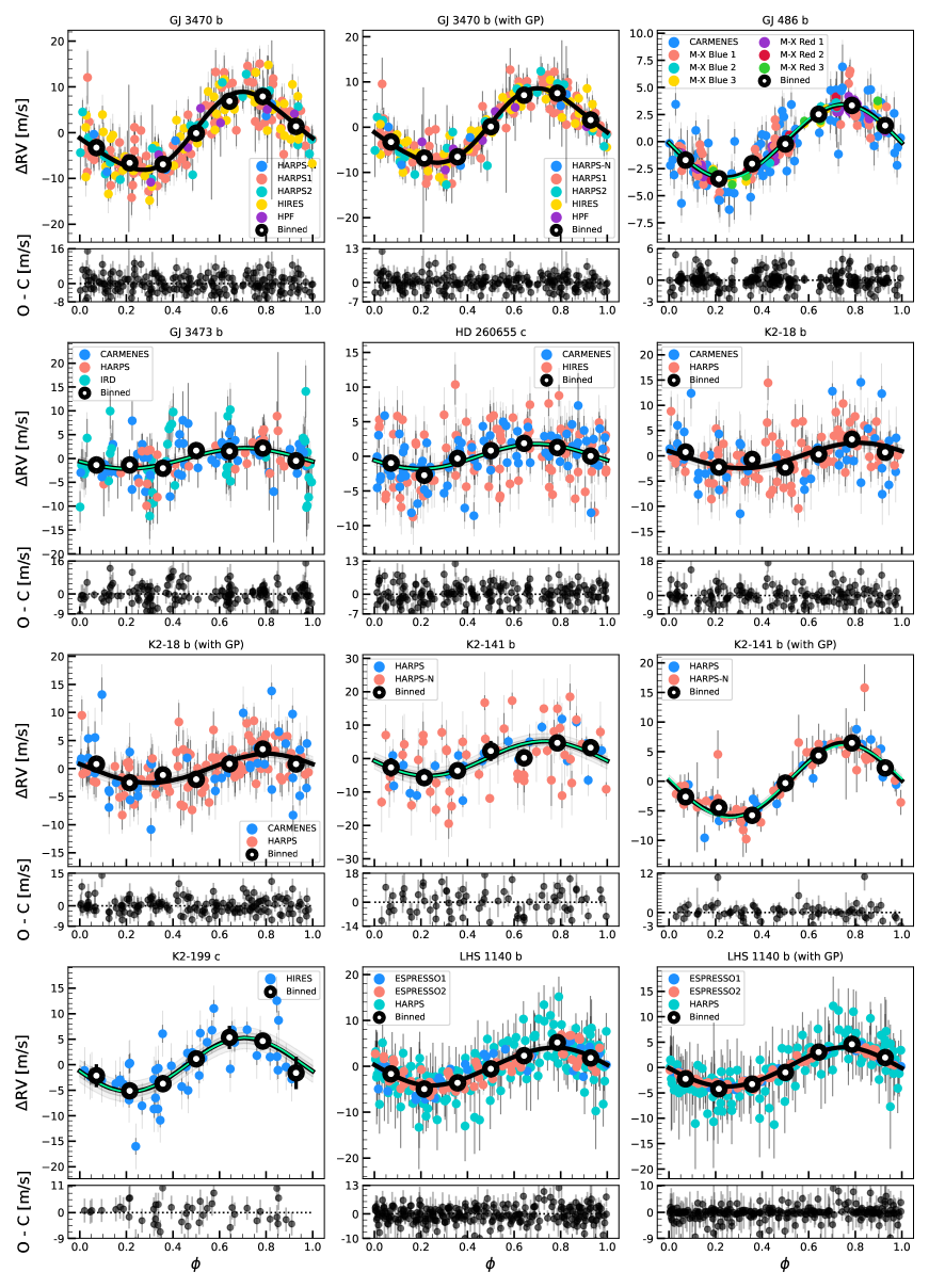
Figure 8: Phase-folded radial velocity curves for the transiting planets ordered by groups as in Table B. The colors of the measurements identify the instrument as shown in each legend. Error bars show the measurement uncertainty (dark grey) and its quadratic sum with the instrument jitter (light grey). Instrument offsets, trends, and GPs have been substracted when required. Black solid line corresponds with the median of the predicted posterior distribution of the model, and the dark and light grey shaded regions are its corresponding 1-$\sigma$ and 2-$\sigma$ intervals. Green line shows the model for the circular case. We assume the trends and GPs of the circular models to be the same as in the eccentric except for TOI-1130 b, for which we separate both cases in different charts.

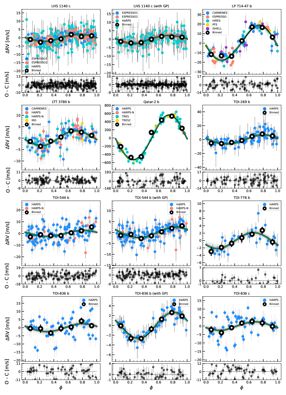
Figure 8: Continuation of the phase-folded radial velocity curves.

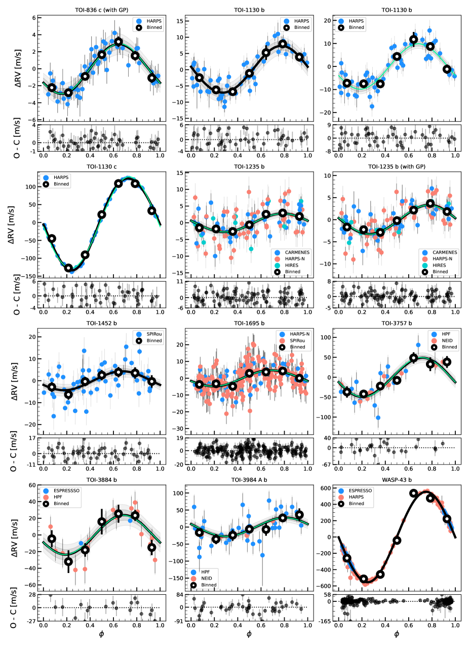
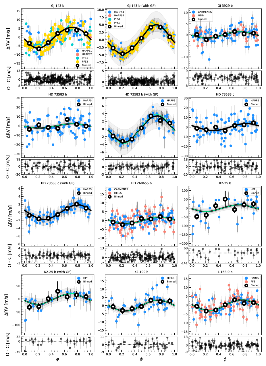
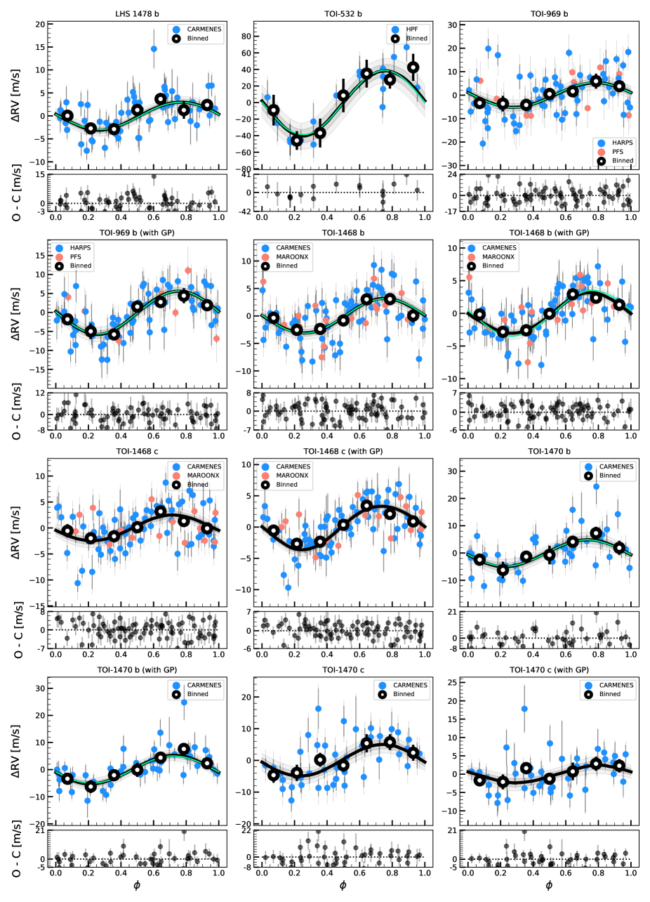
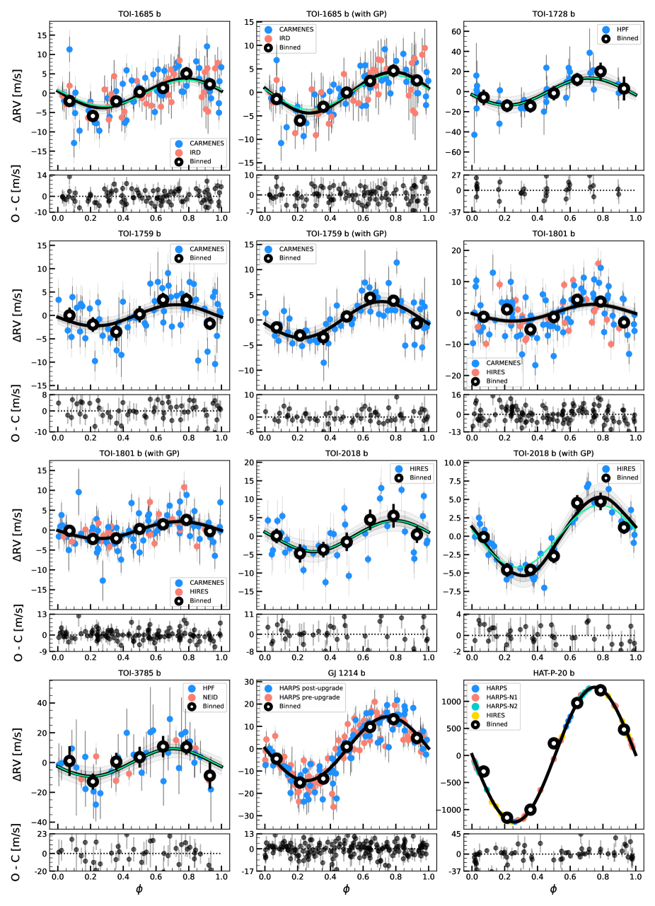
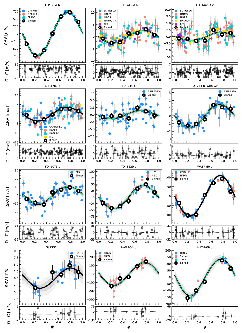
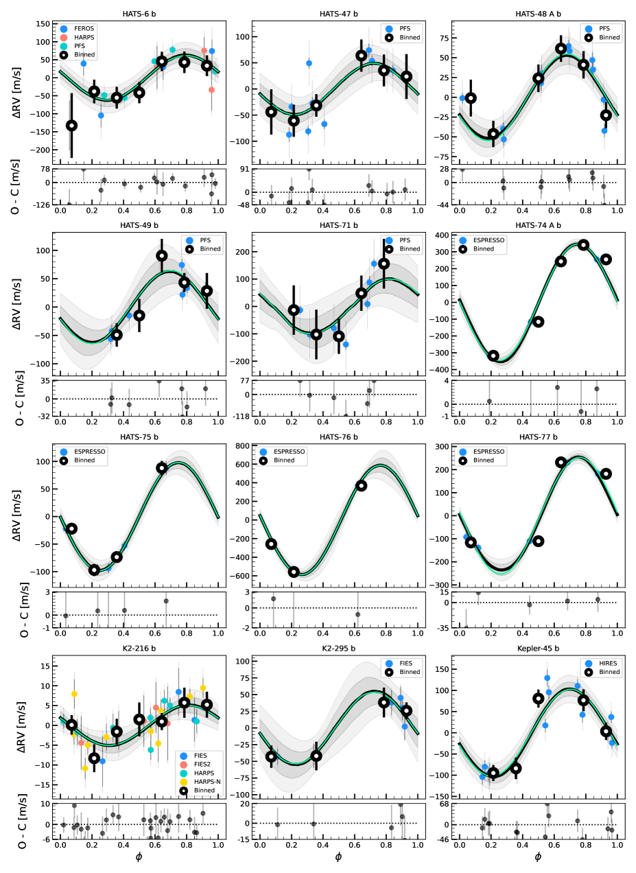
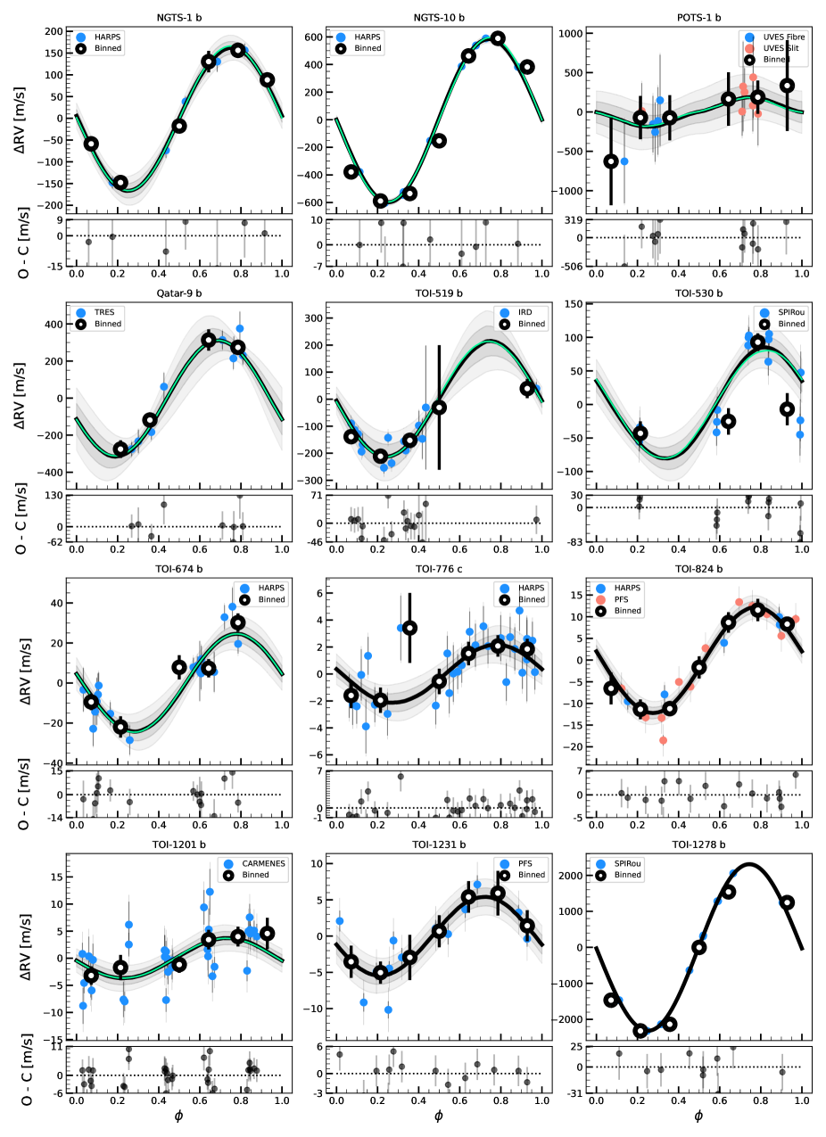
Figure 8: Continuation of the phase-folded radial velocity curves.

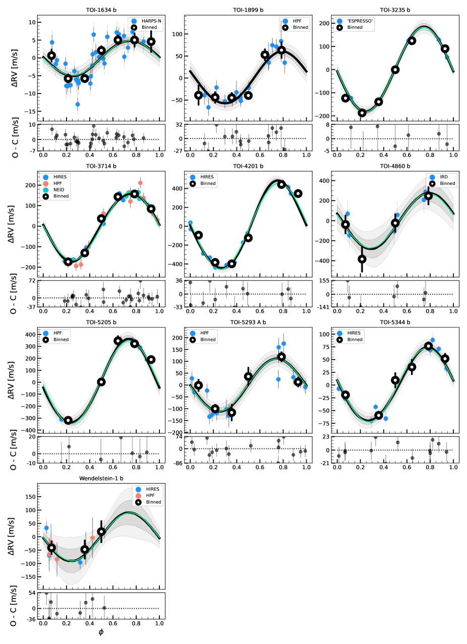
Figure 8: Continuation of the phase-folded radial velocity curves.

Figure 8: Continuation of the phase-folded radial velocity curves.

Figure 8: Continuation of the phase-folded radial velocity curves.

Figure 8: Continuation of the phase-folded radial velocity curves.

Figure 8: Continuation of the phase-folded radial velocity curves.

Figure 8: Continuation of the phase-folded radial velocity curves.

Figure 8: Continuation of the phase-folded radial velocity curves.