The Degree of Fairness in Efficient House Allocation

Abstract.

The classic house allocation problem is primarily concerned with finding a matching between a set of agents and a set of houses that guarantees some notion of economic efficiency (e.g. utilitarian welfare). While recent works have shifted focus on achieving fairness (e.g. minimizing the number of envious agents), they often come with notable costs on efficiency notions such as utilitarian or egalitarian welfare. We investigate the trade-offs between these welfare measures and several natural fairness measures that rely on the number of envious agents, the total (aggregate) envy of all agents, and maximum total envy of an agent. In particular, by focusing on envy-free allocations, we first show that, should one exist, finding an envy-free allocation with maximum utilitarian or egalitarian welfare is computationally tractable. We highlight a rather stark contrast between utilitarian and egalitarian welfare by showing that finding utilitarian welfare maximizing allocations that minimize the aforementioned fairness measures can be done in polynomial time while their egalitarian counterparts remain intractable (for the most part) even under binary valuations. We complement our theoretical findings by giving insights into the relationship between the different fairness measures and conducting empirical analysis.

1. Introduction

The classic house allocation problem is primarily concerned with assigning a set of houses (or resources) to a set of agents based on their preferences over houses such that each agent receives at most one house. It was motivated by a variety of applications such as kidney exchange Roth et al. (2004) or labour market Hylland and Zeckhauser (1979) where agents are initially endowed with houses or houses have to be distributed afresh among agents. While this model was primarily studied for designing incentive compatible mechanisms Svensson (1999); Abdulkadiroğlu and Sönmez (2003) along with some notion of economic efficiency, recent works have shifted focus to the issues of fairness such as envy-freeness (EF), which requires that every agent weakly prefers its allocated house to that of every other agent. An envy-free allocation may not always exist: for example, consider two agents who both like the same house. The fair division literature contains a variety of approximate envy measures (e.g. envy-free up to one Lipton et al. (2004); Caragiannis et al. (2019)) that cannot appropriately be utilized here due to the ‘one house per agent’ constraint.

An orthogonal, but more suitable, approach is measuring the ‘degree of envy’ Chevaleyre et al. (2006) among the agents by counting the number of envious agents or the total aggregate envy experienced. In this vein, recent works have investigated the existence of envy-free house allocations under ordinal preferences Gan et al. (2019), maximum-size envy-free allocation Aigner-Horev and Segal-Halevi (2022), and complete allocations that minimizes the number of envious agents Kamiyama et al. (2021); Madathil et al. (2023) or those that minimize the total aggregate envy among agents Hosseini et al. (2023). Yet, these approaches often take a toll on efficiency notions such as size (the number of allocated agents), utilitarian welfare (the sum of agents’ values), or egalitarian welfare (the value of the worst off agent). The following example illustrates some of these nuances.

Example 0 (Fairness in House Allocation).

Figure 1. An envy-free allocation of maximum size is shown in wavy orange; a minimum #envy complete allocation is shown in dashed green; no envy-free allocation has the maximum welfare $2$; and the allocation in blue achieves minimum #envy among the matchings that has the maximum welfare.

Consider an instance with four agents $\{a_{1},a_{2},a_{3},a_{4}\}$ and five houses $\{h_{1},h_{2},\dots,h_{5}\}$ and binary valuations. For the ease of exposition, we use a graphical representation of the problem as shown in Figure 1, where solid lines indicate an agent has a positive valuation for the house.

A maximum-size envy-free allocation (shown in orange) assigns houses $h_{3}$, $h_{4}$, and $h_{5}$ to agents $a_{1}$, $a_{2}$, and $a_{3}$ respectively. A maximum utilitarian welfare allocation that minimizes the number of envious agents (shown in blue) has two envious agents $a_{3}$ and $a_{4}$, and a utilitarian welfare of two. There is no envy-free allocation with maximum utilitarian welfare. A complete allocation (agent saturating) that minimizes the number of envious agents is shown in green. While the size of the maximum size envy-free allocation is three, both the maximum size envy-free allocation and the envy-free allocation with maximum utilitarian welfare, have zero utilitarian welfare.

Finding a complete allocation that minimizes the number of envious agents (the green allocation in the above example) is shown to be NP-complete Kamiyama et al. (2021) even for binary valuations. Moreover, a maximum-size envy-free allocation proposed by Aigner-Horev and Segal-Halevi (2022) only considers allocations to positive valued houses and returns ‘empty’ otherwise, and the envy-free algorithm proposed by Gan et al. (2019) returns ‘none’ because there is no complete envy-free allocation that assigns every agent to a house it likes. While these observations illustrate the intricate trade-offs between each approach, the relation between these notions and their computational aspects remain unclear.

	max $\mathsf{USW}$	max $\mathsf{ESW}$	allocation size $\geq k$
envy-free (EF)	P (Prop. 4)†	P (Thm. 14)	P (Prop. 4)⋆
min #envy	P (Thm. 5)	NP-c (Thm. 15)	$m>n$: NP-c§ $m\leq n$: P (Thm. 8)
min total envy	P (Thm. 10)	as hard as ($) (Thm. 16)	$m>n$: open ($) $m\leq n$: P (Cor. 12 )‡
minimax total envy	open	NP-c (Thm. 17)	NP-c‡

Table 1. The summary of results for weighted instances with $n$ agents, $m$ houses, and $0\leq k\leq\min\{m,n\}$. P and NP-c refer to polynomial time and NP-complete, respectively. ($) refers to the min total envy complete when $m>n$. Result(s) marked by ^§ is due to Kamiyama et al. (2021), those marked by $\ddagger$ and ^† are shown by Madathil et al. (2023) and Aigner-Horev and Segal-Halevi (2022), respectively for binary valuations, and ^⋆ is the result by Gan et al. (2019) for $k=n$.

1.1. Our Contributions

We consider three well-studied notions of economic efficiency - the size (i..e the number of allocated agents), the utilitarian welfare, and the egalitarian welfare of the allocation. We study these notions under both binary and arbitrary positive valuations and investigate their interaction with various envy fairness measures. These include envy-freeness (EF), minimizing the number of envious agents (min #envy), and minimizing the total envy of all agents (min total envy), and minimizing the total envy of the most envious agent (minimax total envy). Table 1 summarizes our results.

Envy-free allocations.

We show that an envy-free allocation of maximum size can be computed efficiently under binary (Proposition 21) or arbitrary non-negative valuations (Proposition 4). By focusing on welfare-maximizing allocations, we show that, should one exist, finding an envy-free allocation that maximizes utilitarian welfare ($\mathsf{USW}$) or egalitarian welfare ($\mathsf{ESW}$) is computationally tractable (Proposition 4 and Theorem 14, resp.).

Utilitarian welfare.

We show that finding an allocation with min #envy (Theorem 5), or min total envy (Theorem 10), is tractable under the added constraint of maximizing $\mathsf{USW}$. Without the welfare constraint, the former problem has been proven to be NP-hard when we aim to find a complete allocation Kamiyama et al. (2021). Additionally, we analyze the relationship between the size of an allocation and its $\mathsf{USW}$. We obtain polynomial time algorithms for finding min #envy (Theorem 8), min total envy (Corollary 12) complete allocations when $m\leq n$.

Egalitarian welfare.

To complement our study, we consider the well-established Rawlsian notion of egalitarian welfare. We first show that finding an envy-free allocation, when one exists, with maximum $\mathsf{ESW}$ can be done in polynomial time (Theorem 14). We highlight a contrast between egalitarian and utilitarian welfare by showing that when considering allocations that maximize the egalitarian welfare (as opposed to utilitarian ones), finding a min #envy allocation is NP-complete (Theorem 15). Moreover, it is NP-complete to find minimax total envy max $\mathsf{ESW}$ (Theorem 17). Finally, while the computational complexity of finding a complete allocation that minimizes the total envy remains open, we show an intriguing relation to its egalitarian welfare counterpart (Theorem 16) and conclude with complementary experimental observations under randomly generated valuations.

On the technical level, the computational hardness often comes from deciding how to utilize the allocation of “undesirable” houses to improve fairness (i.e., by reducing envy). A house is undesirable for an agent if there exists another house with higher value which is not assigned to any other agent. Intuitively, if an agent likes a house that is available (not assigned to anyone), then the agent does not care about other houses that are less valued. Thus, different variants of the fair house allocation problem remain intractable when undesirable houses can be allocated, e.g., when finding a fair complete allocation and $m>n$, or when finding a fair egalitarian welfare maximizing allocation.

1.2. Related Work

Fairness in house allocations is a well studied problem. House allocations were first studied in social choice where the focus was on finding efficient and strategyproof allocations Roth (1982). As the focus shifted towards fair allocations, increasingly algorithmic approaches were used. Achieving fairness by minimizing the number of envious agents or total envy has been studied previously by Gan et al. (2019); Aigner-Horev and Segal-Halevi (2022); Kamiyama et al. (2021); Madathil et al. (2023). Kamiyama (2021) showed hardness of finding EF solutions for pairwise preferences. Belahcène et al. (2021) studied a relaxed notion called ranked envy-freeness. The hardness and approximability of minimizing total envy was studied for housing allocation problem where agents are located on a graph Hosseini et al. (2024, 2023). The egalitarian allocations have been studied under different names such as the classic makespan minimization problem in job scheduling Lenstra et al. (1990), the Santa Claus problem Bansal and Sviridenko (2006), and in fair allocation of resources Lipton et al. (2004); Bouveret and Lemaître (2016). In these settings the problem of maximizing the egalitarian welfare (worst-off agent) is shown to be NP-hard Bouveret and Lemaître (2016), giving rise to several approximation algorithms Shmoys and Tardos (1993). See Appendix A for an extended discussion on related work. Our setting is crucially different from these works in two ways: in the house allocation problem each agent receives at most one house, and not all houses need to be assigned.

2. Model

An instance of the house allocation problem is represented by a tuple $\langle N,H,V\rangle$, where $N\coloneqq\{1,2,\ldots,n\}$ is a set of $n$ agents, $H\coloneqq\{h_{1},h_{2},\ldots,h_{m}\}$ is a set of $m$ houses, and $V\coloneqq(v_{1},v_{2},\ldots,v_{n})$ is a valuation profile. Each $v_{i}(h)$ indicates agent $i$’s non-negative value for house $h\in H$. Thus, for $i\in N$ the value of a house $h\in H$ is $v_{i}(h)\geq 0$, and $v_{i}(\emptyset)=0$. An instance is binary if for every $i\in N$ and every $h\in H$, $v_{i}(h)\in\{0,1\}$; otherwise it is a weighted instance.

An allocation $A$ is an injective mapping from agents in $N$ to houses in $H$. For each agent $i\in N$, $A(i)$ is the house allocated to agent $i$ given the allocation $A$ and $v_{i}(A(i))$ is its value. Thus, for each $\{i,j\}\subseteq N$, $A(i)\cap A(j)=\emptyset$ and any house is allocated to at most one agent. The set of all such allocations is denoted by $\mathcal{A}$.

Fairness.

Given an allocation $A$, we say that agent $i$ envies $j$ if $v_{i}(A(j))>v_{i}(A(i))$. The amount (magnitude) of this pairwise envy is captured by $\mathsf{envy}_{i,j}(A)\coloneqq\max\{v_{i}(A(j))-v_{i}(A(i)),0\}$. Given an allocation $A$, the total (aggregate) envy of an agent $i$ towards other agents is denoted by $\mathsf{envy}_{i}(A)=\sum_{j\in N}\mathsf{envy}_{i,j}(A)$.

An allocation $A$ is envy-free (EF) if and only if for every pair of agents $i,j\in N$ we have $v_{i}(A(i))\geq v_{i}(A(j))$, that is, $\mathsf{envy}_{i,j}(A)=0$. Since envy-free allocations are not guaranteed to exist, we consider other plausible approximations to measure the ‘degree of envy’ Chevaleyre et al. (2006).

Degrees of envy.

An allocation is min #envy if it minimizes the number of envious agents, i.e. $\min_{A\in\mathcal{A}}\#\mathsf{envy}(A)$, where $\#\mathsf{envy}(A)$ is the number of envious agents, i.e., the size of the set $\{i\in N:\mathsf{envy}_{i,j}(A)>0,\text{for some}\ j\in N\}$.

An allocation is min total envy if it minimizes the total envy of all agents, i.e. $\min_{A\in\mathcal{A}}\mathsf{total\textsc{ }envy}(A)$, where $\mathsf{total\textsc{ }envy}(A)$ is the total amount of envy of allocation $A$ experienced by all agents, i.e., $\mathsf{total\textsc{ }envy}(A)\coloneqq\sum_{i\in N}\mathsf{envy}_{i}(A)$.

An allocation is minimax total envy if it minimizes the maximum aggregate amount of envy experienced by an agent, i.e. $\min_{A\in\mathcal{A}}\max_{i\in N}\mathsf{envy}_{i}(A)$.

In the above measures, an allocation is selected from the set of all feasible allocations $\mathcal{A}$. In the next section we discuss the reason behind restricting the set $\mathcal{A}$ to subsets that satisfy some measures of economic efficiency.

Social Welfare.

Without any measures of social welfare, any empty allocation is vacuously envy-free, and consequently satisfies all four measures of fairness. Hence, we consider three notions of social welfare that measure the economic efficiency of allocations based on their size (number of assigned agents), utilitarian, or egalitarian welfare.

The size $|A|$ of an allocation, $A$, is simply the number of agents that are assigned to a house. An allocation is complete if it either assigns a house to every agent ($N$-saturating) when $m\geq n$, or assigns every house to an agent ($H$-saturating) when $m<n$. Note that completeness is a weak efficiency requirement that does not take agents’ valuations into account.

The utilitarian welfare of an allocation $A$ is the sum of the values of individual agents, i.e. $\mathsf{USW}(A)\coloneqq\sum_{i\in N}v_{i}(A)$. A maximum utilitarian welfare allocation is the one that maximizes the sum of the values, and can be found efficiently by computing a maximum-weight bipartite matching in the induced graph (a bipartite graph on $N\cup H$ where edge weights are given by the valuations $V$).

The egalitarian welfare of an allocation $A$ is the value of the worst off agent among all agents in $N$, that is, $\mathsf{ESW}(A)\coloneqq\min_{i\in N}v_{i}(A)$. A $k$-egalitarian welfare is the value of the worst off agent in a subset $S\subseteq N$ of agents of size $k=|S|$ such that $\mathsf{ESW}(A)\coloneqq\min_{i\in S}v_{i}(A)$.

If it is possible to achieve a positive (non-zero) egalitarian welfare for all agents, any allocation that maximizes the egalitarian welfare (there could be multiple) can be selected. In the special case where every feasible $N$-saturating allocation (allocations of size $n$) has an egalitarian welfare of zero, we look for the largest subset of agents $S\subseteq N$ that can simultaneously receive a positive value, and select an allocation that maximizes the $k$-egalitarian welfare among these agents. In Example 1, a maximum egalitarian welfare allocation has welfare one and size two since any larger subset of agents will result in a egalitarian welfare of zero.

Fairness-Welfare Trade-offs.

Our main objective is to investigate the trade-offs between the four fairness measures and various notions of welfare (i.e. economic efficiency). Thus, for each fairness-welfare pair, we define computational problems in the following way: Given an instance of the house allocation problem, $\langle N,H,V\rangle$, find an allocation $A$ that minimizes unfairness as measured by $F$ within the set of all allocations that maximize an efficiency measure of $E$, where $F$ is min envy, min total envy, minimax envy, or minimax total envy and $E$ is max size, max $\mathsf{USW}$, or max $\mathsf{ESW}$.

Some standard graph theoretic notations and algorithms that we use are provided in Appendix B for easy reference.

3. Maximum Size Envy-free Allocations

We start by considering envy-freeness as our main constraint. The goal is to find an envy-free allocation under various welfare measures. Clearly, an envy-free complete allocation may not always exist. Further, an empty allocation is always an envy-free allocation of size $0$. The first objective is to find an envy-free allocation of maximum size. In other words, among the set of all envy-free allocations we find an allocation that maximizes the number of assigned agents (or houses when $m\leq n$). In their paper Gan et al. (2019) describe an efficient polynomial time algorithm to find an envy-free allocation in ordinal instances. However, they restrict themselves to complete envy-free allocations where all agents are assigned some house. Their algorithm returns ‘empty’ when the number of available houses falls below the number of agents.

Our algorithm relaxes this constraint and returns a maximum size envy-free allocation which need not be complete.

Algorithm description.

Algorithm 1 creates a bipartite graph where each agent is only adjacent to houses that are its most preferred. In other words, if there is an edge between an agent $i$ and a house $h$, then $v_{i}(h)$ is positive and maximum among all houses remaining in the graph. The algorithm proceeds by removing all houses in any inclusion-minimal Hall violators. This process repeats by updating the highest valued house among the remaining houses for each agent, and adding, or retaining, the corresponding edges. After either all houses are considered or no Hall violator is found, the algorithm returns a maximum size allocation which is produced by union of a maximum size matching $M$ in the induced graph $G$ and a maximum size matching in the complement graph $\overline{G}-M$.

The next lemma gives a natural invariant for the algorithm.

Algorithm 1 A maximum size envy-free allocation

0:  A house allocation instance $\langle N,H,V\rangle$

0:  A maximum size envy-free allocation

1:  for each agent $i\in N$ do

2:     Let $h_{i}^{\max}\in\operatorname*{argmax}_{h\in H}v_{i}(h)$

3:  end for

4:  Define $E_{\max}=\{(i,h)|i\in N,h\in H,v_{i}(h)=v_{i}(h_{i}^{\max}),v_{i}(h)>0\}$

5:  Create a bipartite graphs $G=(N\cup H,E_{\max})$

6:  if there exists a Hall violator $(N^{\prime},H^{\prime})$ in $G$ then

7:     Delete $H^{\prime}$ from $H$; removing houses that cause envy.

8:  else

9:     return  Allocation $A$ = union of maximum size matching $M$ in $G$ and a maximum size matching in $\overline{G}-M$.

10:  end if

11:  Go to line 1

Lemma 0.

Given a weighted instance, any house removed by Algorithm 1 cannot be a part of any envy-free allocation.

Theorem 3.

Given a weighted instance, Algorithm 1 returns an envy-free maximum size allocation.

Proof.

First, note that Algorithm 1 runs in polynomial time because every component of the algorithm including finding a inclusion-minimal Hall violator Gan et al. (2019); Aigner-Horev and Segal-Halevi (2022) and computing a maximum size bipartite matching runs in time polynomial in $n$ and $m$. Therefore, it suffices to prove that i) every house removed by the algorithm cannot be contained in any envy-free allocation, and ii) a maximum size bipartite matching returns a maximum size allocation among all envy-free allocations.

Statement (i) immediately follows from Lemma 2 and the fact that each agent’s valuations for the houses unassigned in $M$ is zero. Statement (ii) follows from the observation that Algorithm 1 finds a maximum size matching in the induced graph $G$, where every agent only has edges to its most preferred house among the houses retained, no further edges can be added, and no Hall violators exist.

The unassigned houses and unassigned agents in $M$ are assigned in a maximum matching in $\overline{G}-M$. Thus, no agent or house that is already assigned in $M$ is reassigned. Moreover, since we find a maximum matching in $\overline{G}-M$, it assigns maximum number of agents to the houses they value zero. Thus, the algorithm returns the maximum size envy-free allocation on the instance. ∎

4. Utilitarian Welfare

In this section, we show that fair allocations can be obtained efficiently by introducing a utilitarian welfare constraint and show the connection between complete allocations and welfare maximizing ones when restricting the number of houses.

We begin the section by designing an EF allocation with maximum welfare.

Proposition 0.

Given a weighted instance, an envy-free allocation of maximum $\mathsf{USW}$ can be computed in polynomial time.

Note that while a maximum size envy-free allocation can be computed in polynomial time, finding a complete allocation that minimizes the number of envious agents is NP-hard Kamiyama et al. (2021) (see example given in Figure 1).

4.1. Minimum #Envy

We start by showing that finding a $\mathsf{USW}$-maximizing allocation that minimizes #envy can be done in polynomial time. The algorithm constructs a bipartite graph and uses minimum cost perfect matching Ramshaw and Tarjan (2012). The details of the construction and proofs are relegated to Section D.1.

Theorem 5.

Given a weighted instance, a min #envy max $\mathsf{USW}$ allocation can be computed in polynomial time.

While finding a min #envy complete allocation is shown to be NP-hard even for binary instances Kamiyama et al. (2021), we establish a relation between min #envy complete and min #envy max $\mathsf{USW}$ allocations when $m\leq n$ by extending a minimum envy maximum $\mathsf{USW}$ allocation to a complete allocation.

Proposition 0.

In a binary instance when $m\leq n$, given a min #envy max $\mathsf{USW}$ allocation $A$, a complete allocation $\hat{A}$ can be constructed in polynomial time such that

1. $A$ and $\hat{A}$ has equal $\mathsf{USW}$ and #envy, and

2. $\hat{A}$ has minimum #envy among all complete allocations.

Note that Proposition 6 does not hold for weighted instances as we illustrate by Example 27 in Section D.1. Nevertheless, we show that a min #envy complete allocation can be computed in polynomial time for weighted instances when $m\leq n$. The proof is relegated to Appendix D.

Remark 0.

First, given a maximum size envy-free allocation we cannot ‘append’ it to achieve a min #envy complete allocation even for binary instances. In Example 1, the allocation indicated by orange lines cannot be simply completed to reach the min #envy complete allocation (shown in green). Second, when $m>n$ a min #envy max $\mathsf{USW}$ allocation may leave more agents envious compared to a min #envy complete allocation. In Example 1, the min #envy max $\mathsf{USW}$ allocation indicated by blue leaves two agents envious while the min #envy complete allocation (shown in green) only leaves one agent envious.

Theorem 8.

Given a weighted instance, when $m\leq n$, a min #envy complete allocation can be computed in polynomial time.

Our approach to find a min #envy max $\mathsf{USW}$ allocation heavily relies on the set of $\mathsf{USW}$ maximizing allocations. Next, we discuss two observations about the necessity of utilizing $\mathsf{USW}$ maximizing allocations and restriction on the number of houses.

4.2. Minimum Total Envy

When focusing on total envy of agents, under binary valuations, the total envy can be seen as the number of distinct envy relations between all pair of agents. Whereas in weighted instances, individual values for each assigned houses (and not just pairwise relations) play an important role in computing the total envy.

Example 0.

Consider the weighted instance given in Figure 2. There are two allocations that maximize the $\mathsf{USW}$ with a total welfare of $15$. One allocation (shown in red) leaves three agents envious (namely, $a_{2}$, $a_{3}$, and $a_{4}$) with a total envy of $5$; while another allocation (shown in green) only contains one envious agent ($a_{1}$) and still generates the total envy of $5$.

Figure 2. An example depicting the difference between min #envy and min total envy in $\mathsf{USW}$-maximizing allocations. Red has three envious agents, namely, $a_{2},a_{3},a_{4}$ and green has one envious agent $a_{1}$ but both has total envy five.

This example illustrates that the proposed algorithms for finding min #envy max $\mathsf{USW}$ cannot be readily used for finding min total envy max $\mathsf{USW}$. In Appendix D, we present an example (Example 28) which shows that this challenge persists even for binary instances. Nonetheless, we show that one can achieve a min total envy max $\mathsf{USW}$ allocation in polynomial time by constructing a bipartite graph, similar to the algorithm for min #envy max $\mathsf{USW}$, with a carefully crafted cost function that encode envy and $\mathsf{USW}$ as cost, and utilizing algorithms for finding a minimum cost perfect matching.

Algorithm description.

The algorithm (Algorithm 6 in Section D.2) proceeds by constructing a bipartite graph $G=(N\cup H^{\prime},E)$ where the set $H^{\prime}$ is constructed by adding a set of $n$ dummy houses to the set of houses $H$. That is, $H^{\prime}=H\cup\{h^{i}\mid i\in N\}$. Given an agent $i\in N$ and $h\in H^{\prime}$, we have $(i,h)\in E$ if and only if $h\in H$ and $v_{i}(h)>0$, or $h\in H^{\prime}\setminus H$. We construct a cost function $c$ on edges of $G$. Before we define the cost function we scale the valuations $V$ such that for each agent $i$ and house $h$, if we have that $v_{i}(h)>0$, then $v_{i}(h)\geq 1$. Now we define two components of the cost function $c$, namely, envy component $c_{envy}$ and $\mathsf{USW}$ component $c_{sw}$ such that $c=c_{envy}+c_{sw}$. Let $H^{\max}_{i}$ be the set of most preferred houses in $H$ for agent $i$, i.e., $H^{\max}_{i}=\operatorname*{argmax}_{h\in H}v_{i}(h)$. For ease of exposition we assume $v_{i}(h)=0$ for each agent $i$ and a dummy house $h\in H^{\prime}\setminus H$. For an edge $(i,h)\in E$, if $h\in H^{\max}_{i}$, then define $c_{envy}(i,h)=0$; otherwise $c_{envy}(i,h)=\sum_{\bar{h}\in H}\max\{v_{i}(\bar{h})-v_{i}(h),0\}$. We denote $\sum_{i\in N}\sum_{\bar{h}\in H}v_{i}(\bar{h})+1$ by $L$. Furthermore, we define the $\mathsf{USW}$ component of the cost $c$ for an edge $(i,h)\in E$ as $c_{sw}(i,h)=-v_{i}(h)\cdot L$. Finally, we return a minimum cost perfect matching matching in $G$.

Theorem 10.

Given a weighted instance, a min total envy max $\mathsf{USW}$ allocation can be computed in polynomial time.

Proof Sketch.

Suppose the algorithm (Algorithm 6) returns allocation $A$. Then $A$ corresponds to a minimum cost perfect matching in the constructed graph $G$. We show that by minimizing the cost, we maximize the welfare and minimize the total envy. Observe that the cost of each pair $(i,h)\in A$ has two components, namely, $\mathsf{USW}$ component $-v_{i}(h)\cdot L$ and a envy component. To complete the proof we show that (i) since $L$ is large, a minimum cost matching in $G$ maximizes $\mathsf{USW}$; (ii) the envy component of the cost of a perfect matching correctly computes the total envy of each agent. It follows from the fact that in a max $\mathsf{USW}$ allocation every house valued higher than house $h$ by agent $i$ must be allocated for each $(i,h)\in A$. ∎

We show a result analogous to Proposition 6 holds for min total envy even for weighted instances.

Proposition 0.

Given a weighted instance with $m\leq n$, let $A^{*}$ be a min total envy max $\mathsf{USW}$ allocation. Then a complete allocation $A$ can be constructed in polynomial time such that

1. $A^{*}$ and $A$ has equal $\mathsf{USW}$ and envy, and

2. $A$ is a min total envy complete allocation.

Corollary 12 follows immediately from Proposition 11.

Corollary 0.

Given a weighted instance, a min total envy complete allocation can be computed in polynomial time when $m\leq n$.

Observe that even when $m\leq n$, there may be several complete matchings with different total envy. In Figure 3, both matchings are complete because they assign all the houses, however, the allocation indicated by red yields a higher total envy (two by $a_{2}$) than the green one (one by $a_{3}$).

Figure 3. Two complete allocations with different total envy. Total envy of the red allocation is two due to agent $a_{2}$, the same for green is one due to $a_{3}$.

5. Egalitarian Welfare

When the efficiency measure is maximizing the utilitarian welfare, any maximum-weight matching on the induced bipartite graph returns the required allocation in polynomial time. However, the problem of finding an allocation that maximizes the egalitarian welfare has received less attention in the house allocation setting.

While in fair division finding an allocation that maximizes the egalitarian welfare is NP-hard, we show that in the house allocation setting wherein agents are restricted to receive at most one house, an egalitarian solution can be found in polynomial time.

Note that in binary instances, finding an egalitarian allocation is equivalent to finding an envy-free allocation of maximum size (Proposition 21) since in every allocation the egalitarian welfare is either zero or one. When it comes to weighted instances, however, the goal is to maximize the number of agents who receive a positive value and, conditioned on that, maximize the value of the worst-off agent. We use this intuition to search for an allocation that maximizes the number of agents that receive a positively valued house.

Algorithm 2 Finding an allocation of max $\mathsf{ESW}$

0:  A house allocation instance $\langle N,H,V\rangle$.

0:  An allocation with maximum egalitarian welfare.

1:  for $k=n$ to $1$ do

2:     Let $v_{\max}\coloneqq\max_{i,h}{v_{i}(h)}$ and $v_{\min}\coloneqq\min_{i,h}{v_{i}(h)}$ $\triangleright$ Looping all unique values of houses in $H$

3:     for $\beta=v_{\max}$ to $v_{\min}$ do

4:        Create a bipartite graph $G_{\beta}=(N\cup H,E)$ s.t. there is exists an edge between each agent $i\in N$ and each house $h\in H$ if $v_{i}(h)\geq\beta$

5:        Let $A\coloneqq$ a maximum size matching of $G_{\beta}$

6:        if there exist $k$ allocated agents in $A$ then

7:           return  Allocation $A$

8:        end if

9:     end for

10:  end for

Algorithm description.

The algorithm (Algorithm 2) begins by considering the maximum number of agents $k=n$ who can potentially receive a positively-valued house. Consider the set of all agent valuations in decreasing order. For each such value $\beta$, create a bipartite graph $G_{\beta}$ where there is an edge between any agent-house $(i,h)$ pair if $v_{i}(h)\geq\beta$. Now, find a maximum-size matching $M$ on $G_{\beta}$. If the size of the matching is $k$, the algorithm returns $M$ as the required allocation. Otherwise, it repeats this process by decreasing the size to $k=k-1$.

Theorem 13.

Given a weighted instance, an egalitarian welfare maximizing allocation can be found in polynomial time.

Proof.

Suppose that Algorithm 2 returns an allocation $A$ of size $k$ where every allocated agent receives positive value of at least $\beta$. To prove the theorem we need to show that (i) $k$ is the largest number of agents that can simultaneously receive positive value and (ii) $\mathsf{ESW}(A)$ is maximum among all allocations of size at least $k$. Note that it is sufficient to prove this for size exactly $k$ since we cannot increase $\mathsf{ESW}$ by increasing the size of $A$. Since $A$ is a maximum size matching in $G_{\beta}$, from definition of $G_{\beta}$, it holds that we cannot allocate more than $k$ agents to the houses they value at least $\beta$. Furthermore, the size $k$ decreases from $n$, and the algorithm returns the first $k$-sized allocation where each assigned agent receives positive value. Thus $A$ is the largest possible allocation where each assigned agent gets some positive value since we iterate over all positive values of $\beta$. Thus we show (i). Moreover, since we start by setting $\beta$ to the highest possible value of $\mathsf{ESW}$ and decrease step by step, there does not exist a $k$ size allocation for a higher value of $\beta$. Therefore, for any $k$-sized allocation $\beta$ is the maximum $\mathsf{ESW}$. Thus we show (ii). Note that the possible values of $\beta$ is bounded by the distinct values agents have towards the houses. Then, there are $O(mn)$ values can be assumed by $\beta$. Thus the algorithm runs in polynomial time. ∎

Clearly, a maximum egalitarian allocation may not be unique. Thus, a natural question is whether we can find a fair allocation among all such allocations. We first show that analogous to its utilitarian counterpart (Proposition 4), an envy-free allocation (if one exists) of maximum $\mathsf{ESW}$ can be computed in polynomial time.

Algorithm description.

Given an instance $I=\langle N,H,V\rangle$, Algorithm 3 first finds a max $\mathsf{ESW}$ allocation with welfare at least $\beta$ for $k$ agents using Algorithm 2. Then we find an envy-free allocation, if exists, with egalitarian welfare at least $\beta$ for $k$ agents. We construct a reduced valuation $V^{\prime}$ where $v^{\prime}_{i}(h)$ is set to $v_{i}(h)$ if $v_{i}(h)\geq\beta$ and is zero otherwise for an agent $i\in N$ and house $h\in H$. Then, we invoke Algorithm 1 as a subroutine to find a EF allocation $A$ in $\langle N,H,V^{\prime}\rangle$. If $k$ agents receive value at least $\beta$ in $A$, then we return the allocation $A$; otherwise we return an empty allocation since no EF allocation of max $\mathsf{ESW}$ exists.

Algorithm 3 Finding an EF allocation of maximum $\mathsf{ESW}$

0:  A house allocation instance $\langle N,H,V\rangle$.

0:  An EF allocation with maximum egalitarian welfare.

1:  Let $k$ and $\beta$ denote the size and $\mathsf{ESW}$ of an allocation returned by Algorithm 2.

2:  Create valuation $V^{\prime}$ s.t $v^{\prime}_{i}(h)=v_{i}(h)$ if $v_{i}(h)\!\geq\beta$; $v^{\prime}_{i}(h)\!=\!0$ otherwise, for an agent $i\in N$ and house $h\in H$.

3:  Let $A$ be the allocation returned by Algorithm 1 given $\langle N,H,V^{\prime}\rangle$.

4:  if there exists $k$ allocated agents in $A$ then

5:     return  allocation $A$.

6:  end if

7:  return  $\emptyset$

We prove the correctness of Algorithm 3 in the next theorem.

Theorem 14.

Given a weighted instance, an envy-free allocation of maximum $\mathsf{ESW}$ can be computed in polynomial time.

Proof.

We have the following property of the allocation $A$ returned by Algorithm 3. Each agent that is assigned a house in $A$ receives value at least $\beta$. The statement follows from the facts that each agent is assigned a house that it values positively by Algorithm 1 and each positive value in $V^{\prime}$ is at least $\beta$. However, there may exist agents that is not assigned any house in $A$. Thus, if Algorithm 1 returns an allocation that does not assign $k$ agents, from the definition of maximum egalitarian welfare we conclude that there is no EF allocation of max $\mathsf{ESW}$. The correctness of this step follows from Theorem 3. It shows that in $A$, maximum number of agents are assigned with positive value. So an agent $i$ that is unassigned in the allocation $A$ cannot be assigned to a house it likes without generating envy. Therefore, there is no EF allocation that can match $i$ to a house that it values $\beta$ or more.

Using Theorem 3, we have that allocation $A$ is EF. This completes the proof of correctness of Algorithm 3. Since Algorithms 1 and 2 runs in time polynomial in $n$ and $m$, Algorithm 3 runs in polynomial time. ∎

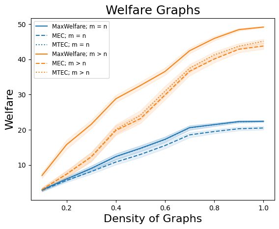
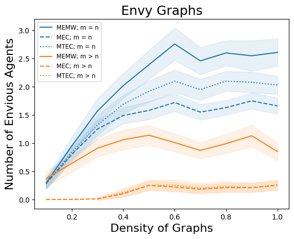
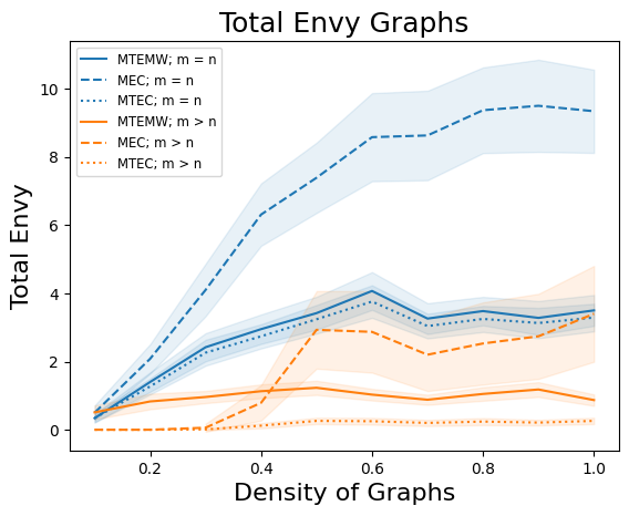
Figure 4. The averages of #envy (number of envious agents), total envy, and $\mathsf{USW}$ over $100$ random trials for each graph density, given $5$ agents and $\{5,10\}$ houses. Codes in the legend refer to MTEC: min total envy complete; MEC: min #envy complete; MEMW: min #envy max $\mathsf{USW}$; MTEMW: min total envy max $\mathsf{USW}$.

5.1. Minimum #Envy

We aim to find an $\mathsf{ESW}$ welfare maximizing allocation that minimizes the number of envious agents. Under binary valuations, the $\mathsf{ESW}$ is either zero or one. When the $\mathsf{ESW}$ is one, we return a complete, envy-free allocation. For $\mathsf{ESW}$ zero, an empty allocation is the optimal solution. In contrast to the utilitarian welfare setting (Theorem 5), finding a max $\mathsf{ESW}$ allocation that is min #envy is intractable in a weighted instance.

Theorem 15.

Given a weighted instance, finding a min #envy max $\mathsf{ESW}$ allocation is NP-hard.

proof sketch.

We prove this by showing a reduction from the problem of finding a min #envy complete allocation that is known to be NP-complete Kamiyama et al. (2021). Given an instance $I=\langle N,H,V\rangle$ of the minimum #envy complete problem, we build an equivalent instance of the min #envy max $\mathsf{ESW}$ problem. For each agent $i\in N$ and house $h\in H$, we create the valuation $v^{\prime}_{i}(h)$ by adding a positive small value $\beta$ to the valuation $v_{i}(h)$. Thus, all max $\mathsf{ESW}$ allocations assign a positively valued house to each agent under the new valuation. We show the hardness of the problems lies in minimizing #envy under the completeness requirement. In Section E.1 we show the equivalence of the two instances to complete the proof. ∎

It is easy to check that the decision version of min #envy max $\mathsf{ESW}$ - where we check if there exists a max $\mathsf{ESW}$ allocation with #envy at most $t$ - is in NP. Thus the problem is NP-complete.

5.2. Minimum Total Envy

While minimizing the total amount of envy experienced by the agents, restricting the search space to the maximum egalitarian welfare allocations does not result in any computational improvement. The problem remains computationally as hard as finding a min total envy complete allocation.

Theorem 16.

Given a weighted instance, finding a min total envy of max $\mathsf{ESW}$ is as hard as finding a min total envy complete allocation.

The proof uses the same construction as in Theorem 15. We defer the details to Section E.2. If in return the objective is to minimize the maximum total of envy experienced by agents (minimax total envy) the problem becomes NP-hard. Note that similar to Theorem 15, in the decision version of the problem, one can check whether minimax total envy of the allocation is at most $t$, implying that the problem is NP-complete.

Theorem 17.

Given a weighted instance, finding a minimax total envy max $\mathsf{ESW}$ allocation is NP-hard.

The detailed proof can be found in the Section E.3. In a nutshell, we provide a reduction from the Independent Set problem in cubic graph Garey and Johnson (1979). Note that even though our construction is similar to Madathil et al. (2023)’s hardness reduction for finding a minmax total envy complete allocation, our reduction further ensures that every agent receives a positive value.

6. Experiments

We experimentally investigate the welfare loss and fairness of the proposes algorithms on randomly generated bipartite graphs. For a fixed number of agents, we varied the number of houses ($m=n$ and $m>n$) and considered both binary and weighted valuation functions $V$. We modelled preferences by iterating over the density of edges ($\lambda\in[0.1,1.0]$), i.e. the probability that an edge exists is $\lambda$, in the corresponding bipartite graph. For each instance, defined by $(m,\lambda,V)$, we ran $100$ trials, on a randomly generated a graph $G$ that satisfied the $(m,\lambda,V)$ constraints. We compared the maximum $\mathsf{USW}$ achieved by a welfare maximizing allocations, to the welfare achieved by an envy minimizing allocation allocations to understand the price of fairness. For the former allocations, we observed min #envy max $\mathsf{USW}$ and min total envy max $\mathsf{USW}$ allocations, and for the latter we considered min #envy complete and min total envy complete allocations. Next, we compared the #envy (and total envy) of min #envy complete (resp. min total envy complete) with that of the min #envy max $\mathsf{USW}$ and min total envy complete (resp. min total envy max $\mathsf{USW}$ and min #envy complete). The plots below show us the average value of these metrics over the $100$ trials for weighted valuations, and highlight the $95\%$-Confidence Interval.

Observations. When there is an abundance of houses, the envy and total envy of all allocations decreases and the $\mathsf{USW}$ increases. Similarly, as the graph grows denser (i.e. $\lambda>0.4$), welfare increases and, under binary valuations, envy and total envy vanish. For weighted valuations too, we notice a slight decrease, but they still persist. As expected, the number of envious agents in a min #envy complete allocation is least, followed by min total envy complete and min #envy max $\mathsf{USW}$. The lower $\mathsf{USW}$ of min total envy complete can be attributed to leaving highly valued houses unallocated. Notably, min #envy complete has higher total envy than min total envy max $\mathsf{USW}$, since it would prefer one highly envious agent to multiple slightly envious ones. Additional plots and discussions on experiments can be found in Appendix F.

7. Concluding Remarks

Our investigation on the tradeoffs between different efficiency and fairness concepts gives rise to several intriguing open questions. For example, the computational complexity of minimizing total envy remains unsolved. Moreover, one can ask if we can guarantee approximations of welfare to achieve EF or relaxations of EF; or whether the complexity of the problems change when considering strict ordinal preferences, Borda valuations, or pairwise preferences.

Supplementary Material

Appendix A Additional Related Work

Gan et al. Gan et al. [2019] described an algorithm to find an envy-free allocation, should one exist, that allocates a house to each agent when the preference of an agent is given as ranking over the houses. They also proved that an EF allocation exists with high probability if the number of houses exceeded the number of agents by a logarithmic factor. Building on this, Aigner-Horev and Segal-Halevi Aigner-Horev and Segal-Halevi [2022] developed an algorithm to find the maximum size EF allocation under binary valuations where agents are only assigned to houses they value positively. Further, for a slightly relaxed definition of envy under weighted valuations, they also found the maximum cardinality EF matching. Madathil et al. Madathil et al. [2023] consider complete allocations, allow assignment of zero-valued house to an agent. Under binary valuations, they study min #envy, min total envy, and minimax total envy allocations and refer to them as optimal, utilitarian, and egalitarian house allocation problems, respectively. They show that minimax total envy complete allocations can be found in polynomial time under restrictions. They show it is NP-hard in general using a reduction from Independent Set [Madathil et al., 2023, Lemma 38] similar to us (Theorem 17).

Kamiyama Kamiyama [2021] considered the problem of finding envy-free allocations for pairwise preferences and showed it is NP-hard even with some restricted preferences, polynomial time with more restrictions, and W[1]-hard parameterized by the number of agents. Belahcene et al. Belahcène et al. [2021] look at the house allocation problem under the guise of project allocations and evaluate a relaxed notion of envy-freeness i.e. rEF where agents are only envious of houses given to another agent if they rank the house higher than the other agent. Hosseini et al. Hosseini et al. [2023] discuss the notion of aggregate envy, where they sum every agent’s pairwise envy with every other agent to create an envy measure they minimize. They prove that even under restricted valuations, i.e. identical and evenly spaced agent valuations, minimizing the amount of aggregate envy is NP-hard by a reduction from the linear arrangements problem. Hosseini et al. Hosseini et al. [2024] define the graphical housing allocation problem as generalization of the minimum linear arrangement and house allocation problem, and characterize the approximability of housing allocation on graphs with different structures.

Appendix B Additional Material from Section 2

B.1. Graphical Representations and Techniques

For completeness, here we define some of the standard definitions in graph theory that we used. Given a bipartite graph $G=(A\cup B,E)$, a matching $M$ is a pairwise vertex disjoint subset of edges $E$. We denote the complement graph of a graph $G$ as $\overline{G}$. We use the notation $G-M$ to denote the reduced graph obtained by deleting the vertices matched in $M$ from $G$.

Definition 0 (Hall Violator).

A Hall set is a subset $A^{\prime}\subseteq A$ such that $|N(A^{\prime})|<|A^{\prime}|$ where $N(A^{\prime})$ denotes the neighbors of vertices in the set $A$, i.e., $N(A^{\prime})=\{v\in B\mid u\in A,(uv)\in E\}$. We call the set $N(A^{\prime})$ as a Hall violator.

A minimal Hall violator can be computed in polynomial time Gan et al. [2019]; Aigner-Horev and Segal-Halevi [2022].

A matching $M$ is maximal when it is not contained in any other matching. A maximum matching in a graph $G$ is a matching containing maximum number of edges in $G$.

Definition 0 (Maximum Size allocation in $G$).

A maximum size bipartite matching in $G=(A\cup B,E)$ is the largest matching between the sets $A$ and $B$ formed by the union of a maximum size matching $M$ in $G$ and a maximum size matching in $\overline{G}-M$.

Note that any maximum size allocation in a graph $G=(N\cup H,V)$ can be found in polynomial time, since it is the union of two maximum size matchings which can each be found in polynomial time.

Given a bipartite graph $G=(A\cup B,E)$ with a cost function $c:E\mapsto\mathcal{R}$, the minimum cost perfect matching problem (also known as the assignment problem) is to find a matching $M$ that matches all vertices of the smaller size and minimizes the cost $\sum_{e\in M}c(e)$. Then, a minimum cost perfect matching matching can be found in strongly polynomial time using Hungarian method Ramshaw and Tarjan [2012].

Graphical representation of house allocation. Given an instance $\langle N,H,V\rangle$, we construct a bipartite graph $G=(N\cup H,E)$ such that given $i\in N$ and $h\in H,(i,h)\in E$ if and only if $v_{i}(h)>0$. We call $G$ as the valuation graph. When the valuations are not binary, we additionally construct an edge weight function $wt$ defined as: $wt((i,h))=v_{i}(h)$ for $i\in N$, $h\in H$, and $(i,h)\in E$. Given an allocation $A$ of $\langle N,H,V\rangle$, we define the matching corresponding to allocation $A$ in $G$ as the set of vertex disjoint edges $\{(i,h)\in E\mid i\in N,h\in H,\text{ and }A(i)=h\}$.

Appendix C Material Omitted From Section 3

C.1. Binary Valuations

When the valuations of agents towards houses are binary, there is a polynomial time algorithm that can return an envy-free allocation of maximum size (or empty) by computing an “envy-free matching” on the bipartite graph induced by the house allocation instance Aigner-Horev and Segal-Halevi [2022]. However, as we illustrated in Example 1, while an envy-free maximum size ‘matching’ of Aigner-Horev and Segal-Halevi [2022] may return ‘empty’, an envy-free allocation of maximum size could be of larger size.

The key difference between our approach is that we allow allocations along zero edges (aka houses that are valued zero and are not adjacent).

We start by providing some structural results in binary instances. The next proposition consolidates two key ideas presented in Theorem 1.1 (e) and Theorem 1.2 of Aigner-Horev and Segal-Halevi [2022] on finding envy-free matchings. We, then, use it to prove Proposition 21.

Proposition 0 (Aigner-Horev and Segal-Halevi [2022]).

Every bipartite graph $G=(N\cup H,E)$ admits a unique partition of $N=N_{S}\cup N_{L}$ and of $H=H_{S}\cup H_{L}$ such that every envy-free matching in $G$ is contained in $G[N_{L},H_{L}]$, a maximum matching in $G[N_{L},H_{L}]$ is a maximum envy-free matching in $G$, and it can be computed in polynomial time.

We will use Proposition 20 to prove the following proposition.

Proposition 0.

Given a binary instance, an envy-free allocation of maximum size can be computed in polynomial time.

Proof.

Given a binary instance $\langle N,H,V\rangle$, we start by constructing a bipartite graph $G=(N\cup H,E)$ such that given $i\in N$ and $h\in H,(i,h)\in E$ if and only if $v_{i}(h)=1$. We do the following:

1. Find a envy-free matching $M$ by using Proposition 20. Add all (agent, house) pairs in $M$ to $A$.

2. While there exists an unassigned (agent, house) pair $(j,h)$ in $A$ such that each agent $i$ with valuation $v_{i}(h)>0$ is matched in $M$, we add the pair $(j,h)$ to $A$.

We show that $A$ is envy-free. By Proposition 20, $M$ is envy-free. Therefore, no envy is created in step (1). Let $(j,h)$ be a pair assigned in the step (2) of the algorithm. No agent can be envious of $j$ since each agent $i$ that likes the house $h$ is assigned to another house it likes in step (1), i.e., for an agent $i$, if $v_{i}(h)>0$, then we have that $v_{i}(A(i))=1$. Since this holds true for each iteration of step (2), allocation $A$ is envy free.

Now we show that $A$ is of maximum size. Towards this, first note that every EF allocation matches only the houses in $H_{L}$ (from Proposition 20). Thus it suffices to show that maximum possible houses in $H_{L}$ are allocated in $A$. Observe that each house in $H_{L}$ satisfies the premise for step (2) since $M$ is a maximum matching in $G[N_{L}\cup H_{L}]$. Therefore, step (2) of our algorithm allocates houses in $H_{L}$ as long as there is an unassigned agent. Therefore, $A$ has maximum size. Thus, $A$ a maximum size EF. ∎

The above algorithm is based on binary bipartite matchings, and thus, it fails to work when we allow for more expressive preferences beyond binary instances. Nonetheless, we develop a polynomial time algorithm to find maximum size allocations with zero envy in the next section.

C.2. Weighted Instances

See 2

Proof.

Suppose for contradiction that there exists a house $h$ that is removed by Algorithm 1 that can be assigned to agent $i$ under an envy-free allocation $A$. If $h$ is deleted in Algorithm 1, then it must be included in a Hall violator $X$ - which means all agents in $X$ cannot be assigned to the houses in $X$. There must then exist an agent $j\in X$ that does not receive its most preferred house $h$ - or any house of equal value - despite it being assigned to some other agent. All houses $h^{\prime}$ with a positive valued edge to agent $j$, added to $E$ in later steps of Algorithm 1 must satisfy $v_{j}(h^{\prime})<v_{j}(h)$, since we add edges in decreasing order of preference. Clearly any allocation where $h$ is assigned leaves $j$ envious, regardless of the house agent $j$ may later receive from a maximum size allocation on $G$.

Thus, given a Hall violator $X$ in the graph $G$, no house $h\in X$ can be contained in an envy-free allocation. ∎

Next we present the complete proof of Theorem 3.

See 3

Proof.

First, note that Algorithm 1 runs in polynomial time because every component of the algorithm including finding a inclusion-minimal Hall violator Gan et al. [2019]; Aigner-Horev and Segal-Halevi [2022] and computing a maximum size bipartite matching runs in time polynomial in $n$ and $m$. Therefore, it suffices to prove that i) every house removed by the algorithm cannot be contained in any envy-free allocation, and ii) a maximum size bipartite matching on the induced graph returns a maximum size allocation among all envy-free allocations.

Let $A$ denote the allocation returned by the algorithm. Statement (i) immediately follows from Lemma 2. Statement (ii) follows from the observation that Algorithm 1 finds a maximum size bipartite matching in the induced graph where every agent only has edges to its most preferred houses in the remaining instance.

First let us consider the agents that receive a house that they value positively. Note that a maximum size bipartite matching in $G$ first finds a maximum matching in $G$. In a maximum-size matching on $G$, an assigned agent is given a house it values most in $G$ and no further assignment to a positively valued house is possible.

Next consider the agents that receive a zero valued house in $A$. A maximum size bipartite matching in graph $G$ will assign the remaining agents (that cannot be assigned in a maximum size matching in $G$) to zero valued houses while such a house is available. Thus the algorithm assigns maximum number of agents to their positively valued houses in $G$ and maximum number of agents to their zero valued houses in $G$.

Recall that since there is no Hall violator in $G$ and a house deleted from $G$ is never assigned, by Lemma 2 the maximum size bipartite matching does not create envious agents. Thus, it returns the maximum size envy-free allocation on the instance. ∎

Given a weighted instance $\langle N,H,V\rangle$ we first show how to find a maximum welfare allocation among all the EF allocations in polynomial time using Algorithm 1.

Lemma 0.

An allocation $A$ returned by Algorithm 1 is a maximum utilitarian welfare EF allocation in $\langle N,H,V\rangle$.

Proof.

Allocation $A$ is envy-free by design. We show that it has maximum $\mathsf{USW}$ among the EF allocations. Let $N_{1}\subseteq N$ denote the set of agents that has non-zero value for some house in $G$ when $A$ is returned by Algorithm 1. First we show that each agent $i\in N_{1}$ receives their highest valued house in $G$. Then, we show that no higher valued house can be assigned to any agent. Thus, we show that an agent cannot receive a higher valued house in an EF allocation. Consequently, $A$ must have maximum welfare among the EF allocations.

Clearly, since there are no Hall violators in $G$, we have that allocation $A$ allocates a house to each agent in $N_{1}$. Moreover, if $(i,h)$ is an edge in $G$, then, since the allocation is EF, $h$ is a highest valued house for $i$ among the houses that were not deleted. Thus, if an agent $i\in N_{1}$ receives a house $h$ in allocation $A$, then house $h$ is a highest valued house for $i$ in $G$.

Next we show a higher valued house cannot be assigned in to an agent in any EF allocation. Suppose that an agent $i$ receives a house $h$ (recall, $h=\emptyset$ when $i$ does not receive a house) in $A$. Let $h^{\prime}$ be a house that has higher value for $i$. Since we add the edges in decreasing order of value in $G$ and $v_{i}(h^{\prime})>v_{i}(h)$, the house $h^{\prime}$ must have been added to $G$ and removed by the algorithm. Then, using Lemma 2, we have that $h^{\prime}$ cannot be assigned in any EF allocation. Finally, since $A$ is maximum size allocation in Algorithm 1, by Definition 19 no agent can receive a higher valued house.

Thus, welfare of $A$ is maximum among the EF allocations. ∎

Observe that if there exists an EF allocation among the ones with maximum $\mathsf{USW}$, then we can find that using Lemma 22 by checking if the allocation has maximum welfare.

See 4

Proof.

From Theorem 3 we have that $A$ is an EF matching. In Lemma 22, we prove that $A$ is of maximum welfare among the envy-free allocations. If $\mathsf{USW}(A)$ is the same as the maximum utilitarian welfare of an allocation in the given instance $\langle N,H,V\rangle$, then we return $A$; otherwise we return ‘No’. Since $\mathsf{USW}(A)$ is the maximum welfare achieved by any EF allocation, the correctness of this step follows. Thus, we show the proposition. ∎

Appendix D Material Omitted From Section 4

D.1. Minimum #Envy

Given an instance $\langle N,H,V\rangle$, we construct an instance of minimum cost perfect matching that we later use to solve min #envy max $\mathsf{USW}$.

Algorithm description

We construct a bipartite graph $G(N\cup H^{\prime},E)$ from $I=\langle N,H,V\rangle$, on vertex set $N\cup H^{\prime}$ where the set $H^{\prime}$ is constructed by adding a set of $n$ dummy houses to the set of houses $H$, i.e., $H^{\prime}=H\cup\{h^{i}\mid i\in N\}$. For an agent $i\in N$ and house $h\in H^{\prime}$, the pair $(i,h)\in E$ if and only if house $h\in H$ and $v_{i}(h)>0$, or $h\in H^{\prime}\setminus H$. We define a cost function $c:E\mapsto\mathcal{R}$ on edges of $G$. For ease of exposition we assume $v_{i}(h)=0$ for each agent $i$ and a dummy house $h\in H^{\prime}\setminus H$. Before we define the cost function we scale the valuations $V$ such that for each agent $i$ and house $h$, if we have that $v_{i}(h)>0$, then $v_{i}(h)\geq 1$. Now we define cost function $c$ as follows:

• for each agent $i$ and house $h\in H^{\prime}$ we define $c(i,h)=0$ if $h$ belong to the set of houses with highest value for agent $i$, and otherwise $c(i,h)=1$. We call this as the envy component of cost and write it as $c_{envy}(i,h)$.

• for each edge $(i,h)$ in $G$ such that $h\in H$, we add $-v_{i}(h)\cdot L$ to $c(i,h)$ where $L=n+1$. We call this as the welfare component of cost and write is as $c_{sw}(i,h)$.

Thus, the cost of an edge $c(i,h)$ in $G$ is $c_{sw}(i,h)+c_{envy}(i,h)$, as given in Algorithm 4.

This completes the construction of the graph $G$. Finally, we return a minimum cost perfect matching matching in $G$ as a min #envy max $\mathsf{USW}$ allocation.

Algorithm 4 a min #envy max $\mathsf{USW}$ allocation

0:  A house allocation instance $\langle N,H,V\rangle$.

0:  An allocation of maximum $\mathsf{USW}$ that minimizes the number of envious agents.

1:  Create a bipartite graph $G=(N\cup H^{\prime},E)$ s.t. $H^{\prime}=H\cup\{h^{i}\mid i\in N\}$ and $(i,h)\in E$ if $v_{i}(h)>0$, or $h\in H^{\prime}\setminus H$ for an agent $i\in N$ and a house $h\in H^{\prime}$.

2:  Let $c:E\mapsto\mathcal{R}$ be defined as follows for an edge $(i,h)\in E$:

$$c(i,h)=\begin{cases}-v_{i}(h)\!\cdot\!L&\textit{if $h\in H$ is a most preferred house}\\ &\lx@algorithmic@hfill\textit{ for agent $i$,}\\ -v_{i}(h)\!\cdot\!L\!+\!1\!&\textit{otherwise}\\ \end{cases}$$

where $L=n+1$.

3:  return  a minimum cost perfect matching matching in $G$.

We begin by observing some properties of cost a matching in $G$. For a matching $M$ in $G$ we write $c(M)$ to denote $\sum_{(i,h)\in M}c(i,h)$ and define $c_{sw}(M)$ and $c_{envy}(M)$ analogously. Note that $c(M)=c_{sw}(M)+c_{envy}(M)$.

Lemma 0.

Let $M$ be a perfect matching in $G$. Then $c_{envy}(M)\leq n$.

Proof.

Note that for each agent $i\in N$ the cost $c_{envy}(i,h)$ is at most $1$ for all $h\in H^{\prime}$. Since $M$ is a matching of size at most $n$, $c_{envy}(M)\leq n$. ∎

We define an allocation $A_{M}$ from a matching $M$ in $G$ as follows: for each edge $(i,h)\in M$ such that $h\in H$, assign house $h$ to $i$ in $A_{M}$. The rest of the agents remain unassigned in $A_{M}$. Then the following lemma follows from the definition of $c_{sw}$.

Lemma 0.

Let $M$ be a matching in $G$. Then $\mathsf{USW}(A_{M})=-\frac{1}{L}c_{sw}(M)$.

Proof.

Recall that for each edge $(i,h)\in M$ such that $h\in H$, cost $c_{sw}(i,h)=-v_{i}(h)L$ and we assign house $h$ to $i$ in $A_{M}$. Therefore, for each edge $(i,h)\in M$, we add welfare $-c_{sw}(i,h)/L$ to the utilitarian welfare of $A_{M}$. Thus, $\mathsf{USW}(A_{M})=\sum_{(i,h)\in M}-c_{sw}(i,h)/L=-\frac{1}{L}\sum_{(i,h)\in M}c_{sw}(i,h)=-\frac{1}{L}c_{sw}(M)$. ∎

Finally we are ready to prove the theorem. See 5

Proof.

To prove the theorem we first observe that Algorithm 4 runs in polynomial time since construction of $G$ and finding a minimum cost perfect matching matching can be done in polynomial time. Next, we prove the correctness of the algorithm.

Let $M^{*}$ be a minimum cost perfect matching in $G$. First we show that $A_{M^{*}}$ is a maximum-welfare allocation. Then we will show that it has minimum number of envious agents.

Suppose that there exists an allocation $M^{\prime}$ such that $\mathsf{USW}(M^{\prime})>\mathsf{USW}(M^{*})$. Then the following calculations give us a contradiction to the fact that $M^{*}$ has minimum cost in $G$. The first inequality follows since for any house $h$ that is liked by agent $i$, we have that $v_{i}(h)\geq 1$.

$$\mathsf{USW}(M^{\prime})-1 \geq\mathsf{USW}(M^{*})$$

$$-\mathsf{USW}(A_{M^{\prime}})+1 \leq-\mathsf{USW}(A_{M^{*}})$$

$$-\mathsf{USW}(A_{M^{\prime}})\cdot L+L \leq-\mathsf{USW}(A_{M^{*}})\cdot L$$

In the next line, we replace welfare by $c_{sw}$ using Lemma 24 and replace $L$ by $c_{envy}(M^{\prime})$. Then the inequality changes to strict since using Lemma 23, envy of any matching is less than $n<L$.

$$-c_{sw}(M^{\prime})\cdot L+c_{envy}(M^{\prime}) <c_{sw}(M^{*})\cdot L$$

The next line follows since $c_{envy}(M^{*})$ is non-negative.

$$-c_{sw}(M^{\prime})\cdot L+c_{envy}(M^{\prime}) <c_{sw}(M^{*})\cdot L+c_{envy}(M^{*})$$

$$c(M^{\prime}) <c(M^{*}).$$

The final inequality follows from the definition of cost function. Hence, we get a contradiction. Thus, $A_{M^{*}}$ has maximum $\mathsf{USW}$.

Given that $A_{M^{*}}$ has maximum $\mathsf{USW}$, we show that number of envious agents in $A_{M^{*}}$ is minimum.

Lemma 0.

An agent $i$ is envious in the allocation $A_{M^{*}}$ if and only if it is not assigned to one of its most preferred houses.

Proof.

Suppose agent $i$ is envious, then clearly it is not assigned to its most preferred house. We prove the other direction. Suppose $i$ is not assigned to any of its most preferred houses. Let $h$ be a most preferred house for agent $i$. We prove that $i$ is envious due to $h$ by showing $h$ assigned in $A_{M^{*}}$, i.e., $h$ is matched in $M^{*}$. We have that $v_{i}(h)>v_{i}(M^{*}(i))$ since $h$ is a most preferred house and $M^{*}(i)$ is not. Moreover, $c(i,h)=-v(i,h)L$ and $c(i,M^{*}(i))=-v(i,M^{*}(i))L+1$ from the construction of the cost function. Thus, $c(i,h)<c(i,M^{*}(i))$. Therefore, if $h$ is not matched in $M^{*}$, then replacing $(i,M^{*}(i))$ by $(i,h)$ in $M^{*}$ decreases its cost, contradicting the fact that $M^{*}$ has minimum cost. Thus, we prove that agent $i$ is envious. ∎

Therefore, using Lemma 25 and from the construction of the cost function, an agent adds $1$ to $c_{envy}(M^{*})$ if and only if it is envious. Hence, the cost $c_{envy}(M^{*})$ in $G$ is the number of envious agents in $A_{M^{*}}$ in $I$.

To complete the proof, we need to show that $M^{*}$ minimizes the cost $c_{envy}$ in $G$. Suppose towards contradiction there exists a perfect matching $M^{\prime}$ in $G$ such that $A_{M^{\prime}}$ has maximum welfare in $I$ and $c_{envy}(M^{\prime})<c_{envy}(M^{*})$ in $G$. Then, from Lemma 24, we have that $c_{sw}(M^{\prime})=c_{sw}(M^{*})$ since both $A_{M^{\prime}}$ and $A_{M^{*}}$ has maximum $\mathsf{USW}$. Therefore, $c_{sw}(M^{\prime})+c_{envy}(M^{\prime})<c_{sw}(M^{*})+c_{envy}(M^{*})$. Thus, we get $c(M^{\prime})<c(M^{*})$, contradicting the fact that $M^{*}$ is a minimum cost perfect matching in $G$. Since $M^{*}$ has minimum $c_{envy}$, allocation $A_{M^{*}}$ minimizes the number of envious agents among all maximum welfare allocations. ∎

See 6

Proof.

We begin the proof by constructing a complete allocation $\hat{A}$ in time polynomial in $m$ and $n$. We set $\hat{A}=A$. Then we proceed from $A$ iteratively: add a pair $(i,h)$ to $\hat{A}$ where agent $i$ and house $h$ are unassigned in $\hat{A}$, until $\hat{A}$ is complete.

We show that $\#\mathsf{envy}(\hat{A})=\#\mathsf{envy}(A)$. Let $H_{u}$ be the set of unassigned houses in $A$. We show that assignment of a house in $H_{u}$ does not create more envious agents than in $A$. First, observe that for each agent $i\in N$ and each house $h\in H_{u}$, we have $v_{i}(h)\leq v_{i}(A(i))$ (recall, $v_{i}(A(i))=0$ when $i$ is unassigned). Otherwise, if $v_{j}(h)>v_{j}(A(j))$ for some agent $j$ and $h\in H_{u}$, then we increase the welfare of $A$ by adding $(j,h)$ to $A$ and removing $(j,A(j))$ from $A$, contradicting the fact that $A$ has maximum welfare. Therefore, no agent envy an house $h\in H_{u}$ that is assigned in the iterative step. Then the envy of each agent remains the same as in $A$ after the iterative step. Thus, $\#\mathsf{envy}(\hat{A})=\#\mathsf{envy}(A)$.

Next, we prove that $\mathsf{USW}(A)=\mathsf{USW}(\hat{A})$. It is clear from the construction that $\mathsf{USW}(\hat{A})\geq\mathsf{USW}(A)$ since we assign more houses in $\hat{A}$. Observe that each agent $i$ that is assigned a house $h$ in $H_{u}$ receives utility zero; otherwise, we could add $(i,h)$ to $A$ to increase its welfare. Therefore, $\mathsf{USW}(\hat{A})=\mathsf{USW}(A)$. This completes the prove of (i).

We prove (ii) by contradiction. Suppose that there exists a min #envy complete allocation $A^{*}$ such that $\#\mathsf{envy}(A^{*})<\#\mathsf{envy}(A)$. Then, let $j$ be an agent that is envious in $A$ but not in $A*$. Then, from the fact that the valuations are binary, we have $v_{j}(A^{*}(j))=1$ since all houses are assigned in $A^{*}$ as $m\leq n$ and $j$ is not envious in $A^{*}$. Additionally, $v_{j}(A(j))=0$ since $j$ is envious in $A$. Therefore, each agent that is envious in $A$ but not in $A^{*}$ adds one to $\mathsf{USW}(A^{*})$ and zero to $\mathsf{USW}(A$). The converse holds true as well. If $v_{i}(A(i))=1$ and $v_{i}(A^{*}(i))=0$ for an agent $i$, then $i$ must be envious in $A^{*}$ but not in $A$ due to binary valuations. Therefore, more agents add one to the welfare of $A^{*}$ than that of $A$ since $A$ has more envious agents than $A^{*}$. Thus, we get that $\mathsf{USW}(A^{*})>\mathsf{USW}(A)$, a contradiction to the fact that $A$ has maximum welfare.

∎

As a consequence of Theorem 5 and Proposition 6 we get the following.

Corollary 0.

Given a binary instance, a min #envy complete can be computed in polynomial time when $m\leq n$.

Example 0 (Proposition 6 does not hold for weighted instances).

Consider three houses and three agents as shown in Figure 5. The values are shown on edges. The min #envy max $\mathsf{USW}$ allocation shown in red must allocate $h_{1}$ to $a_{1}$ with the value of $100$ to satisfy the maximum $\mathsf{USW}$ constraint. This allocation results in creating two envious agents (agents 2 and 3). However, The min #envy complete allocation (shown in green) has exactly one envious agent.

Figure 5. The min #envy max $\mathsf{USW}$ allocation (shown in red) is not a min #envy complete allocation (shown in green) in weighted instances.

Algorithm 5 Finding a min #envy complete allocation when $m\leq n$

0:  A house allocation instance $\langle N,H,V\rangle$ with $m\leq n$.

0:  A min #envy complete allocation $A$.

1:  Create a bipartite graph $G_{\max}=(N\cup H,E_{\max})$ where $(i,h^{\max}_{i})\in E_{\max}$ if and only if $h^{\max}_{i}\in\operatorname*{argmax}_{h\in H}v_{i}(h)$

2:  Let $M$ be a maximum size matching in $G_{\max}$.

3:  Initialize $A=M$

4:  while there exists a unassigned house $h$ in $A$ do

5:     Allocate $h$ to an unassigned agent in $A$.

6:  end while

7:  return  Allocation $A$.

Observe that each house is assigned in every complete allocation when $m\leq n$. Thus, if an agent is assigned to its most preferred house, then it cannot be envious of others. On the other hand, each agent that doesn’t receive its most preferred house (or one from such set) is envious of some agent. This gives us the following characterization.

Claim 1.

When $m\leq n$, in any complete allocation an agent is not envious if and only if it is assigned to one of its most preferred houses.

Based on the above characterization, we design Algorithm 5.

Algorithm description

In Algorithm 5, given an weighted instance $\langle N,H,V\rangle$, we construct an unweighted bipartite graph $G_{\max}=(N\cup H,E_{\max})$ such that given $i\in N$ and $h\in H$, we have $(i,h)\in E_{\max}$ if and only if $h$ is a most preferred houses of agent $i$. We find a maximum size matching $M$ in the graph $G_{\max}$. We extend $M$ to construct a complete allocation $A$ as follows: initialize $A=M$; until $A$ is complete, allocate an unassigned house to an unassigned agent in $A$.

We prove the correctness of Algorithm 5 in the next theorem. See 8

Proof.

Let $A$ be the allocation produced by Algorithm 5. We show that $A$ has minimum envy among the set of complete allocations of $\langle N,H,V\rangle$.

Suppose that there is a complete allocation $A^{*}$ with $\#\mathsf{envy}(A^{*})<\#\mathsf{envy}(A)$. We obtain a matching $M^{*}$ from $A^{*}$ as follows: $M^{*}=\{(i,A^{*}(i))\mid i\in N\textit{ and $i$ is envy-free in $A^{*}$}\}$. We show that $M^{*}$ is a matching in $G_{\max}$ and has more edges than $M$, a contradiction to the fact that $M$ is of maximum size.

First, we show $M^{*}$ is a matching in $G_{\max}$. By using 1 for $A^{*}$, we have $A^{*}(i)$ is a most preferred house for each envy-free agent $i$. Thus, from definition of $E_{\max}$, we have that $(i,A^{*}(i))\in E_{\max}$ for each envy-free agent $i$ in $A^{*}$. Therefore, $M^{*}$ is a matching in $G_{\max}$. Next, we show size of $M$ is strictly less than that of $M^{*}$. From 1, if an agent is matched in $M$, then it is envy-free in $A$. Thus, the number of edges in $M$ is strictly less than that of $M^{*}$ since number of envy-free agents in $A$ is strictly less than that of $A^{*}$. Therefore, we get a contradiction to the fact that $M$ is a maximum size matching in $G_{\max}$ and prove that $A$ is a min #envy complete.

The matching $M$ can be found in time $O(m\sqrt{n})$ using a maximum size matching algorithm Hopcroft and Karp [1973] and extending $M$ to $A$ takes time $O(m+n)$. ∎

D.2. Minimum Total Envy

Example 0 (Example showing min #envy max $\mathsf{USW}$ does not imply min total envy max $\mathsf{USW}$ even in binary instances).

Consider the instance given in Example 1. The allocation shown in blue, that is, $(a_{1},h_{1})$ and $(a_{2},h_{2})$ maximizes the welfare and leaves only two agents envious $\{a_{3},a_{4}\}$. Similarly, allocation $(a_{3},h_{1})$ and $(a_{4},h_{2})$ maximizes the welfare and leaves two agents envious. Yet, the former has a total envy of 2, while the latter has a total envy of 3.

We find a min total envy max $\mathsf{USW}$ allocation by finding a minimum cost perfect matching allocation in an appropriately constructed graph. The construction is similar to the one finding min #envy max $\mathsf{USW}$ allocation with a different cost function as given in Algorithm 6.

Algorithm 6 A min total envy max $\mathsf{USW}$ allocation

0:  A house allocation instance $\langle N,H,V\rangle$.

0:  An allocation of maximum $\mathsf{USW}$ that minimizes the total envy of agents.

1:  Create a bipartite graph $G=(N\cup H^{\prime},E)$ s.t. $H^{\prime}=H\cup\{h^{i}\mid i\in N\}$ and $(i,h)\in E$ if $v_{i}(h)>0$, or $h\in H^{\prime}\setminus H$ for an agent $i\in N$ and a house $h\in H^{\prime}$.

2:  Let $H^{\max}_{i}$ be the set of most preferred houses in $H$ for agent $i$.

3:  Define $c:E\mapsto\mathcal{R}$ for an edge $(i,h)\in E$ as follows:

$$c(i,h)=\begin{cases}-v_{i}(h)\cdot L,\lx@algorithmic@hfill\textit{\hskip 151.76964pt if }h\in H^{\max}_{i}&\\[3.87498pt] -v_{i}(h)\cdot L+\sum_{\bar{h}\in H}\max\{v_{i}(\bar{h})-v_{i}(h),0\}&\\ \lx@algorithmic@hfill\textit{\hskip 216.81ptotherwise}&.\end{cases}$$

where $L=\sum_{i\in N}\sum_{\bar{h}\in H}v_{i}(\bar{h})+1$.

4:  return  a minimum cost perfect matching matching in $G$.

The proof will be analogous to the proof of Theorem 5. We being with some properties of a minimum cost perfect matching in $G$.

Lemma 0.

Let $M$ be a perfect matching in $G$. Then $c_{envy}(M)<L$.

Proof.

Note that for each agent $i\in N$ the cost $c_{envy}(i,h)$ is at most $\sum_{\bar{h}\in H}v_{i}(\bar{h})$ for any house $h$. Therefore, for all the agents in $N$ the total envy component of the cost $c_{envy}(M)\leq\sum_{i\in N}\sum_{\bar{h}\in H}v_{i}(\bar{h})$. Since $L=\sum_{i\in N}\sum_{\bar{h}\in H}v_{i}(\bar{h})+1$, we have that $c_{envy}(M)<L$. ∎

The next lemma follows from the definition of $c_{sw}$ and the proof is the same as Lemma 24.

Lemma 0.

Let $M$ be a matching in $G$. Then $\mathsf{USW}(A_{M})=-\frac{1}{L}c_{sw}(M)$.

Now we are ready to proof the correctness of Algorithm 6.

See 10

Proof.

Let $M$ be a matching in $G$. We define

$$A_{M}=\{(i,M(i))\mid M(i)\in H\}\cup\{(i,\emptyset)\mid M(i)\in H^{\prime}\setminus H\}$$

Let $M^{*}$ be a minimum cost perfect matching in $G$. We show that $A_{M^{*}}$is a min total envy max $\mathsf{USW}$ allocation where $M^{*}$ is a minimum cost perfect matching in $G$. The proof will be analogous to the proof of Theorem 5. First we show that $A_{M^{*}}$ is a maximum-welfare allocation. Then we will show that it has minimum total envy of the agents.

The proof to show that $A_{M^{*}}$ is a maximum-welfare allocation is the same as in Theorem 5 except we use Lemmas 30 and 29 to reach a contradiction. We show it below for the sake of completeness.

Suppose that there exists an allocation $M^{\prime}$ such that $\mathsf{USW}(M^{\prime})>\mathsf{USW}(M^{*})$. Then the following calculations give us a contradiction to the fact that $M^{*}$ has minimum cost in $G$. The first inequality follows since for any house $h$ that is liked by agent $i$, we have that $v_{i}(h)\geq 1$.

$$\mathsf{USW}(M^{\prime})-1 \geq\mathsf{USW}(M^{*})$$

$$-\mathsf{USW}(A_{M^{\prime}})+1 \leq-\mathsf{USW}(A_{M^{*}})$$

$$-\mathsf{USW}(A_{M^{\prime}})\cdot L+L \leq-\mathsf{USW}(A_{M^{*}})\cdot L$$

In the next line, we replace welfare by $c_{sw}$ using Lemma 30 and replace $L$ by $c_{envy}(M^{\prime})$. Then the inequality changes to strict since using Lemma 29, envy of any matching is strictly less than $L$.

$$-c_{sw}(M^{\prime})\cdot L+c_{envy}(M^{\prime}) <c_{sw}(M^{*})\cdot L$$

The next line follows since $c_{envy}(M^{*})$ is non-negative.

$$-c_{sw}(M^{\prime})\cdot L+c_{envy}(M^{\prime}) <c_{sw}(M^{*})\cdot L+c_{envy}(M^{*})$$

$$c(M^{\prime}) <c(M^{*}).$$

The final inequality follows from the definition of cost function. Hence, we get a contradiction. Thus, $A_{M^{*}}$ has maximum $\mathsf{USW}$.

Given that $A_{M^{*}}$ has maximum $\mathsf{USW}$, we show that the total envy of agents in $A_{M^{*}}$ is minimum.

Lemma 0.

Total envy of an agent $i$ in the allocation $A_{M^{*}}$ is
$c_{envy}(i,M^{*}(i))$.

Proof.

To prove the statement we consider each of the three cases in the definition of $c_{envy}$.

If $M^{*}(i)$ is a highest valued house for agent $i$, then $i$ receives its most preferred house and total envy of $i$ is zero. Form definition of $c_{envy}$, we have $c_{envy}(i,M^{*}(i))=0$ as $M^{*}(i)$ is a most preferred house.

If $M^{*}(i)$ is a dummy house, i.e., $M^{*}(i)\in H^{\prime}\setminus H$, then agent $i$ is not assigned any house in $A_{M^{*}}$. Then $i$ is envious of all the houses it values more than zero. Thus, value of each house $h\in H$ is added to the total envy of $i$. Therefore, total envy of $i$ is $\sum_{h\in H}v_{i}(h)$, the same as defined in the cost $c_{envy}(i,M^{*}(i))$.

Finally, if $M^{*}(i)$ is neither a most preferred house, nor a dummy house, then we claim that agent $i$ is envious of each house that is valued more than $M^{*}(i)$. Let $h$ denote the house $M^{*}(i)$. Let $\bar{h}$ denote a house such that $v_{i}(\bar{h})>v_{i}(h)$. We show that agent $i$ is envious of $\bar{h}$ in $A_{M^{*}}$. Towards this we show that $\bar{h}$ is assigned to some agent in $A_{M^{*}}$. Suppose that $\bar{h}$ is not assigned to any agent in $A_{M^{*}}$, then we can assign agent $i$ to $\bar{h}$ and increase welfare of $A_{M^{*}}$, contradicting the fact that $A_{M^{*}}$ is a max welfare allocation. Therefore, $\bar{h}$ is assigned in $A_{M^{*}}$ and agent $i$ envies $\bar{h}$. Thus, it adds $v_{i}(\bar{h})-v_{i}(h)$ to total envy of $i$ for each $\bar{h}$ such that $v_{i}(\bar{h})>v_{i}(h)$. Observe that this is the same as the cost $c_{envy}(i,M^{*}(i))$. Thus we complete the proof of the lemma. ∎

Therefore, the cost $c_{envy}(M^{*})$ in $G$ is the sum of $c_{envy}(i,M^{*}(i))$ for each agent $i$ since $M^{*}$ is a perfect matching. Therefore, $c_{envy}(M^{*})$ is the same as total envy of agents in $A_{M^{*}}$ in $I$.

To complete the proof, we need to show that $M^{*}$ minimizes the envy component of cost $c_{envy}$ in $G$. Suppose towards contradiction there exists a perfect matching $M^{\prime}$ in $G$ such that $A_{M^{\prime}}$ has maximum welfare in $I$ and $c_{envy}(M^{\prime})<c_{envy}(M^{*})$ in $G$. Then, from Lemma 30, we have that $c_{sw}(M^{\prime})=c_{sw}(M^{\prime})$ since both $A_{M^{\prime}}$ and $A_{M^{*}}$ has the same welfare. Therefore, $c_{sw}(M^{\prime})+c_{envy}(M^{\prime})<c_{sw}(M^{*})+c_{envy}(M^{*})$. Thus, we get $c(M^{\prime})<c(M^{*})$, contradicting the fact that $M^{*}$ is a minimum cost perfect matching in $G$. Since $M^{*}$ has minimum $c_{envy}$, allocation $A_{M^{*}}$ minimizes the total envy of agents among all maximum welfare allocations.

∎

See 11

Proof.

First, note that since $m\leq n$, every house must be allocated to some agent. Any min total envy max $\mathsf{USW}$ allocation $A^{*}$ is complete when every house in $H$ is wanted by at least one agent. Otherwise, we can simply create a complete allocation $A$ from $A^{*}$ as follows. Till there is an unassigned house $h$, assign $h$ to some unassigned agent. Note that completing the allocation does not change the total envy i.e., $\mathsf{total\textsc{ }envy}(A)=\mathsf{total\textsc{ }envy}(A^{*})$. Moreover, it is clear that $A$ and $A^{*}$ has the same welfare.

We prove that $A$ is a min total envy complete allocation by contradiction. Suppose that $A^{*}$ is a min total envy complete allocation such that total envy of $A^{*}$ is less than that of $A$. Then, clearly, welfare of $A^{*}$ must be less than welfare of $A$. Then there exists at least one house $h\in H$ such that agent $i=A(h)$, agent $i^{*}=A^{*}(h)$, and $v_{i}(h)>v_{i^{*}}(h)$.

We show that there exists an agent $z$ such that $\mathsf{envy}_{z}(A)>\mathsf{envy}_{z}(A^{*})$ and there is an alternating path from $h$ to $z$ (the edges of the path are alternating between edges of $A^{*}$ and $A$). Suppose not. Then consider the longest alternating path $P$ (edges alternating between $A^{*}$ and $A$) starting with $i^{*},h,i,A^{*}(i)$ and so on. Construct the allocation $A^{\prime}$ from $A^{*}$ by changing the assignment of each agent in $P$ according to $A$. Then the total envy of the allocation $A^{\prime}$ decreases from total envy of $A^{*}$ since there is no agent $z$ on the path satisfy the condition $\mathsf{envy}_{z}(A)>\mathsf{envy}_{z}(A^{*})$ and total envy of agent $i$ decreases. Thus, we contradict the fact that $A^{*}$ has minimum total envy by constructing $A^{\prime}$. Hence, there is an alternating path from house $h$ to an agent $z$ such that $\mathsf{envy}_{z}(A)>\mathsf{envy}_{z}(A^{*})$. Let $z$ denote the first agent on the aforementioned path from $h$ satisfying $\mathsf{envy}_{z}(A)>\mathsf{envy}_{z}(A^{*})$ and the total envy of the agents path from $h$ to $z$ is less in $A^{*}$ than in $A$. We denote the path by $P_{hz}$.

However, now we construct an allocation $A^{\prime\prime}$ by modifying $A$ along the path $P_{hz}$, i.e., for each agent $j$ on the path $P_{hz}$, we change $A^{\prime\prime}(j)$ from $A(j)$ to $A^{*}(j)$. The total envy of allocation $A^{\prime\prime}$ is less than $A$ since the total envy of the agents path from $h$ to $z$ is less in $A^{*}$ than in $A$. Consequently, the sum of the their values for the assigned houses is more in $A^{*}$ than in $A$. Therefore, the total welfare contributed by the agents on path $P_{hz}$ is increased. Since the remaining assignments are the same as in $A$, we have that $\mathsf{USW}(A^{\prime\prime})$ is more than that of $A$, a contradiction. Thus, the proposition holds.

Thus when $m\leq n$, any decrease in welfare corresponds to an increase in total envy. This means that given a min total envy max $\mathsf{USW}$ allocation, we can retrieve a min total envy complete allocation when $m\leq n$.

∎

Appendix E Omitted proofs from Section 5

E.1. Minimum #Envy

See 15

Proof.

We prove this by showing a reduction from the problem of finding a min #envy complete allocation that is known to be NP-complete.

Let $I=\langle N,H,V\rangle$ be an instance of the Minimum Envy Complete problem where the goal is to find a complete allocation with at most $z$ envious agents. We build an equivalent instance $I^{\prime}=\langle N,H,V^{\prime}\rangle$ of the min #envy max $\mathsf{ESW}$ problem. We create the valuation $V^{\prime}$ as follows:

• for each agent $i\in N$ and house $h\in H$, we set the value $v^{\prime}_{i}(h)=v_{i}(h)+\beta$, where $0<\beta<\min_{(i,h)\in N\times H}v_{i}(h)$.

We now show that an allocation with $\mathsf{ESW}$ at least $\beta$ for all $n$ agents has envy at most $z$ in the instance $\langle N,H,V^{\prime}\rangle$ if and only if a minimum envy complete allocation has envy at most $z$ in $\langle N,H,V\rangle$.

Before we show the equivalence, we show the following property.

Let $A$ be a min #envy max $\mathsf{ESW}$ allocation with $\mathsf{ESW}{}\geq\beta$ in $I^{\prime}$ with $\#\mathsf{envy}(A)\leq z$. We show that the $\mathsf{envy}(A)$ in $I$ and $I^{\prime}$ are the same. The egalitarian welfare of $A$ is at least $\beta>0$., i.e., $v_{i}(A(i))\geq\beta$ for each agent $i$. Then, if an agent $i\in N$ is envious, then $i$ must be envious of an agent who is assigned to a house $h$ such that $v_{i}(h)>\beta$, since there are more houses than agents, and in $I^{\prime}$ each agent has positive valued for all the houses Therefore, if an agent is envious in $I^{\prime}$, then it must be envious in $I$. Thus, each envious agent in $I^{\prime}$ is envious in $I$ for the allocation $A$. Further, if agent $i$ is envious due to a house $h$ in $I$, then it is envious in $I^{\prime}$ since from the construction $\beta\leq v^{\prime}_{i}(h)<v_{i}(h)$ for $(i,h)\in N\times H$. Hence, in the allocation $A$, the number of envious agents in $I$ is the same as in $I^{\prime}$. Hence, $A$ has envy at most $z$ in $I$.

To show the equivalence, first note that a a min #envy max $\mathsf{ESW}$ allocation $A$ is a complete allocation and has minimum envy due to the above property. Hence, $A$ is a min #envy complete allocation with $\mathsf{envy}(A)\leq z$ in $\langle N,H,V\rangle$.

For the other direction, let $A^{\prime}$ be a min #envy complete with $\#\mathsf{envy}(A^{\prime})\leq z$. We show that $\mathsf{ESW}(A^{\prime})\geq\beta$ in $I^{\prime}$. This holds since, by construction, $I^{\prime}$ is a complete graph where every agent has value at least $\beta$ for each house.

Thus any complete allocation in $I$ satisfies the $\mathsf{ESW}$ threshold $\beta$ in an allocation of size $n$ i.e. any min #envy complete allocation in $I$ must also be a min #envy max $\mathsf{ESW}$ allocation in $I^{\prime}$. Since the minimum #envy complete matching is a NP-hard Kamiyama [2021], we conclude that minimum #envy max egalitarian is also NP-hard. ∎

E.2. Minimum Total Envy

See 16

Proof.

Let $\langle N,H,V\rangle$ be an instance of a minimum total envy complete problem. We use the construction in Theorem 15 to construct an instance of min total envy max $\mathsf{ESW}$. First we show the following property. We now show that a minimum total envy allocation $A$ in $\langle N,H,V^{\prime}\rangle$ of size $n$ and $\mathsf{ESW}(A)\geq\beta$ has the same total envy with respect to the valuations $V$ and $V^{\prime}$. We use $G$ and $G^{\prime}$ to denote the two bipartite graphs on vertex set $N\cup H$ where the edges in $G$ and $G^{\prime}$ are given by the valuations $V$ and $V^{\prime}$, respectively. We know that the egalitarian welfare must be at least $\beta>0$. It follows that any envious agent $i\in N$ must be envious of some house it values strictly more than $\beta$. From the construction of the instance we have that each edge that contributes to total envy of an agent $i$ in $G^{\prime}$ exists in $G$. Thus, the total envy of each agent is the same in $G$ and $G^{\prime}$. Hence, if the total envy is minimized in $G^{\prime}$, it must also be minimized in $G$ i.e. a min total envy max $\mathsf{ESW}$ allocation gives us a min total envy complete allocation.

Now we show the equivalence between the instances. A minimum total envy allocation $A$ in $G^{\prime}$ of size $n$ and $\mathsf{ESW}\geq\beta$, is a complete allocation in $G$. Due to the above argument, $A$ has minimum total envy. Hence, $A$ is a min total envy complete allocation in $G$.

For the other direction, given a minimum total envy complete allocation $A$ in $G$, it must have egalitarian welfare $\mathsf{ESW}(A)\geq\beta$ in $G^{\prime}$ since by construction, $G^{\prime}$ is a complete graph where each edge has weight at least $\beta$. Thus, $A$ is an allocation in $G^{\prime}$ of size $n$ and $\mathsf{ESW}\geq\beta$. Therefore, using the above property $A$ is a min total envy max $\mathsf{ESW}$ allocation in $G^{\prime}$. Thus any complete matching in $G$ satisfies the $\beta$-threshold for egalitarian welfare, for size $=n$ i.e. any minimum total envy complete matching in $G$ is a min total envy max $\mathsf{ESW}$ allocation in $G^{\prime}$. ∎

E.3. Minimax Total Envy

See 17

Proof.

The construction of the reduction is the same as in  [Madathil et al., 2023, Lemma 38] except for the valuation functions. We reduce from the Independent Set problem in cubic graph which is known to be NP-hard Garey and Johnson [1979].

We construct an instance $\langle N,H,V\rangle$ of minimax total envy max $\mathsf{ESW}$ from an instance $G=(X,E),k$ of Independent Set where the goal is to find an independent set of size at least $k$. Let $|X|=\hat{n}$ and $|E|=\hat{m}$.

Houses: For each vertex $x\in X$ create a house $h_{x}$, we refer to them as vertex-houses and denote by $H_{X}$. Additionally, we add $3\hat{m}+\hat{n}-k$ dummy houses to $H$.

Agents: For each vertex $x\in X$ create an agent $a_{x}$, we refer to them as vertex-agents and denote by $N_{X}$. For each edge $e\in E$ create three agents $a_{e}^{1},a_{e}^{2},$ and $a_{e}^{3}$, we refer to them as edge-agents. That is, $N=N_{X}\cup\{a_{e}^{1},a_{e}^{2},a_{e}^{3}:e\in E\}$.

Valuations: For each $x\in X$, $v_{a_{x}}(h_{x})=\beta+1$ and $v_{a_{x}}(h)=\beta$ for every house $h\in H\setminus\{h_{u}\}$. For each $e=\{x,y\}\in E$ and each $i\in[3]$, we set $v_{a_{e}^{i}}(h)$ to be $\beta+1$ if $h\in\{h_{x},h_{y}\}$ and set it to be $\beta$ otherwise. This finishes the construction.

First observe that value of an agent towards a house is at least $\beta$. Thus any allocation of the instance has egalitarian welfare at least $\beta$. Now the the proof is the same as [Madathil et al., 2023, Lemma 38].

We prove that $G$ has an independent set of size at least $k$ if and only if $\langle N,H,V\rangle$ has an allocation where maximum $\mathsf{total\textsc{ }envy}{}$ of any agent is at most one. For the forward direction, suppose that $X^{\prime}\subseteq X$ is an independent set in $G$ of size at least $k$. Then, in the following allocation has each agent has $\mathsf{total\textsc{ }envy}{}$ one. We assign the pair $(a_{x},h_{x})$ for each $x\in X^{\prime}$ and assign the remaining unassigned agents to dummy houses. The later step is possible since $|X^{\prime}|\geq k$, so there are at most $\hat{n}-k$ vertex-agents that are not assigned to their corresponding vertex-houses and $3\hat{m}$ edge agents that are unassigned. Now, observe that no vertex agent is envious since either it is assigned to the house it values the most, or it is assigned to the second best house and its best valued the house is not assigned to any agent. Moreover, for each edge-agent, the $\mathsf{total\textsc{ }envy}{}$ is at most one. It follows from the fact that $X^{\prime}$ is an independent set and so both endpoints of an edge is not present in $V^{\prime}$. Hence, for an edge $e=\{x,y\}\in E$, we have that at most one of the houses $h_{x}$ or $h_{y}$ is assigned to their corresponding vertex-agent but both are not assigned. Hence, the edge-agents for $a_{e}^{i}$ has $\mathsf{total\textsc{ }envy}{}$ at most one for $i\in[3]$.

For the other direction, first we show that any allocation that has maximum $\mathsf{total\textsc{ }envy}{}$ at most one can be changed into a nice allocation such that the $\mathsf{total\textsc{ }envy}{}$ of the maximum envious agent remain the same. Here, an allocation is nice if for every assigned vertex-house $h_{x}$ it holds that the agent assigned to $h_{x}$ is $a_{x}$. Suppose it doesn’t hold for some allocation $A$. Then, we add $(a_{x},h_{x})$ and $(A(h_{x}),A(a_{x}))$ to $A$ and delete $(a,A(a_{x}))$ and $(a(h_{x}),h_{x})$ from $A$. The maximum $\mathsf{total\textsc{ }envy}{}$ experienced by any agent remains the same. If the agent $A(h_{x})$ is not an edge-agent such that $v$ is one of the endpoint of the edge, then envy of $A(h_{x})$ does not increase.

Otherwise, let the edge be $e=\{x,y\}$ and wlog, $a_{e}^{1}$ is assigned to $h_{y}$ in $A$. The agent $a_{e}^{1}$ envies only $a_{y}$ after the exchange. This follows from the fact that both $a_{e}^{2}$ and $a_{e}^{3}$ cannot be assigned to $h_{x}$ that is the only other highest valued house for them. Then at least one of them will envy both $A(h_{y})$ and $A(h_{x})$, producing a $\mathsf{total\textsc{ }envy}{}$ of two and contradicting the fact that maximum $\mathsf{total\textsc{ }envy}{}$ is one for any agent in $A$. Hence, we assume we have a nice allocation. Now, the set of vertex-houses assigned to vertex-agents form an independent set in $G$. This completes the proof. ∎

Appendix F Omitted details from Experiments - Section 6

	Utilitarian $\mathsf{USW}$	Min #envy	Min total envy
Binary
Truncated Borda valuations

F.1. Design

Our code was compiled with Python $3.8$ and we use the NetworkX library to model all instances of the house allocation problem as bipartite graphs. We deconstruct our experiments into instances and trials. We fix the number of agents across all instances and trials to be $n=5$.

Instances

An instance $I$ of the problem is defined by the tuple $(m_{I},\lambda_{I},V_{I})$, where $m_{I}$ is the number of houses, $\lambda_{I}$ is the probability that an edge $(a,h)$ between $a\in N$ and $h\in H$ exists, and $V_{I}$ is the type of valuation function. We vary the number of houses ($m_{I}$) over the set $\{n,1.6n,2n\}$ where $n$ is the number of houses, to capture the impact of an abundance of houses on the fairness-efficiency trade-off.

Similarly, $\lambda_{I}$ iterates over the $10$ values in the interval $[0.1,1]$ with step size $=0.1$. Since all edges are picked independently, $\text{Pr}[(a,h)\in G|a\in N,h\in H]=\lambda_{I}$ implies that $\frac{\#\text{ edges in }G}{\max(\text{possible edges in }G)}=\lambda_{I}$. Correspondingly, we choose to refer to $\lambda_{I}$ as the density of the graph.

Lastly, we consider the following three distinct valuation functions:

• Binary Valuations : Each existing edge has weight $=1$ i.e. for all $a\in N,h\in H$ if $\exists(a,h)\in G$ then $v_{a}(h)=1$.

• Weighted Valuations : We noticed a great deal of noise when weighted valuations were uniformly assigned over the interval $[1,100]$ since agent preferences could differ wildly. To minimize this noise while still retaining the fundamental traits that make Weighted Valuations more challenging than Binary Valuations, we assigned each edge $(a,h)\in G$, $v_{a}(h)=k$ for some random $k\in[\text{MaxDeg}(G),\text{MaxDeg}(G)-\text{Deg}(a)+1]$ such that $k$ is chosen without replacement. Note that $\text{MaxDeg}(G)$ is the maximum degree of a node in $G$ and $\text{Deg}(a)$ is the degree of agent $a$ i.e., the number of houses it has positive valuations for.

Thus, the experiments are run over a set of $60$ unique instances, and for each $I$, we generate $100$ random trials.

Trials

A trial is a single randomly generated graph $G$ that satisfies the constraints ($m_{I},\lambda_{I},V_{I}$) of a specific instance $I$. Each $G$ was created using the bipartite random graph function in the NetworkX algorithms library, with parameters ”$(n,m,\lambda_{I})$”. Once $G$ is generated, we give the edges $(a,h)\in G$ weights according to $V_{I}$.

Thus, every instance $I$ defines a corresponding family of graphs $S$, and each trial $T$ of $I$ generates a graph $G$ that belongs to $S$.

F.2. Setup

Given an instance $I$, in each trial $T$ of $I$ we find the following allocations min #envy max $\mathsf{USW}$, min total envy max $\mathsf{USW}$, min #envy complete, and min total envy complete using a brute force implementation. For every type of allocation we store the envy, total envy and utilitarian $\mathsf{USW}$ generated for that specific trial. Once we have these statistics for all trials and all instances, we plot the mean and $95\%$-Confidence Interval over $100$ trials for all instances. For clarity, we plot each of these metrics on different figures and group them by valuation function. Below, we have the plots for Binary and Truncated Borda Valuations.

F.3. Observations

We describe the general trends observed in the plots below:

• Abundance of Houses : As the number of houses increases, the #envy and total envy across all three types of allocations decrease, and the utilitarian $\mathsf{USW}$ generated increases. This is consistent with what we expect. An abundance of houses makes it easier to satisfy the demands of all agents since the probability of each agent getting some house allocated to them, i.e. a complete matching, increases. Under binary valuations this increases the number of envy-free agents, and under (positive) weighted valuations this decreases the envy of all envious agents since very few are left unallocated.

• Density of the Graph : Across matchings and valuation profiles, we notice that as the graph grows more connected, i.e., $\lambda_{I}$ increases, the #envy of the graph increases correspondingly. Under binary valuations we note that $\lambda\leavevmode\nobreak\ 0.3$ is roughly when the graph is connected enough to create large amounts of #envy and total envy, but disconnected enough to prevent a complete matching. When $\lambda>0.3$, as agents are increasingly assigned to some house they want, #envy and total envy decrease correspondingly. Both #envy and total envy rapidly drop to $0$ under binary valuations, but remain non-zero under truncated borda valuations. The latter can be explained by the fact that truncated borda valuations are assigned without repetition, and an agent’s most preferred house being assigned to another, still leaves an agent envious and adding to the total envy of an allocation. Again, this is as expected. Envy only occurs when preferences clash, and this can only happen in reasonably dense graphs. However, since we ensure there are at least as many houses as agents, a further increase in the density of the graph increases the number of completely, or partially, satisfied agents, which explains the decrease in the #envy and total envy.

• #Envy: The envy of a min #envy max $\mathsf{USW}$ allocation is consistently higher than that of a min #envy complete allocation. This is expected since min #envy complete allows for unassigned highly valued houses and assigning houses to agents that do not want them. However, the notable difference between the #envy generated by these two allocations gives us some insight into the considerable impact this relaxation has on the envy of an allocation. Further, we note that while min total envy complete has lesser #envy than min #envy max $\mathsf{USW}$, which can also be attributed to relaxing the max welfare constraint, min total envy complete also has more #envy than a min #envy complete allocation. This can be explained by the fact that min total envy complete would prefer to distribute envy over multiple agents in order to decrease the net total envy, while min #envy complete would prefer to concentrate all the total envy generated on one incredibly envious agent. This highlights the fundamental incompatibility between the two measures.

• Total Envy: Under binary valuations, when $m=n$ the Total Envy generated by the three types of allocations is roughly equivalent, with min total envy complete lower bounding the total envy in all instances. However when $m>n$, there is hardly any total envy once the graph is dense enough for a complete matching. However, when we consider the truncated borda valuations, we notice that min #envy complete performs significantly worse than both min total envy max $\mathsf{USW}$ and min total envy complete allocations. This further hints at total envy being more dependent on the $\mathsf{USW}$ of an allocation than #envy, and thus being somewhat incompatible with envy under weighted valuations.

• Welfare: The utilitarian welfare generated by an allocation is significantly higher in $\mathsf{USW}$ maximizing allocations, like min #envy max $\mathsf{USW}$ and min total envy max $\mathsf{USW}$, than in envy or total envy minimizing allocations such as min #envy complete and min total envy complete. This can be the explained by the significant positive impact that allowing highly wanted houses to go unassigned, has on the envy/total envy of an allocation.

References

- Abdulkadiroğlu and Sönmez [2003] Atila Abdulkadiroğlu and Tayfun Sönmez. School choice: A mechanism design approach. American economic review, 93(3):729–747, 2003.
- Aigner-Horev and Segal-Halevi [2022] Elad Aigner-Horev and Erel Segal-Halevi. Envy-free matchings in bipartite graphs and their applications to fair division. Information Sciences, 587:164–187, 2022.
- Bansal and Sviridenko [2006] Nikhil Bansal and Maxim Sviridenko. The santa claus problem. In Proceedings of the thirty-eighth annual ACM symposium on Theory of Computing, pages 31–40, 2006.
- Belahcène et al. [2021] Khaled Belahcène, Vincent Mousseau, and Anaëlle Wilczynski. Combining fairness and optimality when selecting and allocating projects. In Proceedings of the Thirtieth International Joint Conference on Artificial Intelligence (IJCAI-21), pages 38–44. International Joint Conferences on Artificial Intelligence Organization, August 2021.
- Bouveret and Lemaître [2016] Sylvain Bouveret and Michel Lemaître. Characterizing conflicts in fair division of indivisible goods using a scale of criteria. Autonomous Agents and Multi-Agent Systems, 30(2):259–290, 2016.
- Caragiannis et al. [2019] Ioannis Caragiannis, David Kurokawa, Hervé Moulin, Ariel D Procaccia, Nisarg Shah, and Junxing Wang. The unreasonable fairness of maximum nash welfare. ACM Transactions on Economics and Computation (TEAC), 7(3):1–32, 2019.
- Chevaleyre et al. [2006] Yann Chevaleyre, Paul E Dunne, Ulle Endriss, Jerome Lang, Michel Lemaitre, Nicolas Maudet, Julian Padget, Steve Phelps, Juan A Rodriguez-Aguilar, and Paulo Sousa. Issues in multiagent resource allocation. Informatica, 30(1):3–32, 2006.
- Gan et al. [2019] Jiarui Gan, Warut Suksompong, and Alexandros A Voudouris. Envy-freeness in house allocation problems. Mathematical Social Sciences, 101:104–106, 2019.
- Garey and Johnson [1979] M. R. Garey and David S. Johnson. Computers and Intractability: A Guide to the Theory of NP-Completeness. W. H. Freeman, 1979.
- Hopcroft and Karp [1973] John E. Hopcroft and Richard M. Karp. An n^5/2 algorithm for maximum matchings in bipartite graphs. SIAM Journal on Computing, 2(4):225–231, 1973.
- Hosseini et al. [2023] Hadi Hosseini, Justin Payan, Rik Sengupta, Rohit Vaish, and Vignesh Viswanathan. Graphical house allocation. In Proceedings of the 2023 International Conference on Autonomous Agents and Multiagent Systems, pages 161–169, 2023.
- Hosseini et al. [2024] Hadi Hosseini, Andrew McGregor, Rik Sengupta, Rohit Vaish, and Vignesh Viswanathan. Tight approximations for graphical house allocation. In Proceedings of the 2024 International Conference on Autonomous Agents and Multiagent Systems, page forthcoming, 2024.
- Hylland and Zeckhauser [1979] Aanund Hylland and Richard Zeckhauser. The efficient allocation of individuals to positions. Journal of Political economy, 87(2):293–314, 1979.
- Kamiyama et al. [2021] Naoyuki Kamiyama, Pasin Manurangsi, and Warut Suksompong. On the complexity of fair house allocation. Operations Research Letters, 49(4):572–577, 2021.
- Kamiyama [2021] Naoyuki Kamiyama. The envy-free matching problem with pairwise preferences. Information Processing Letters, 172:106158, 2021.
- Lenstra et al. [1990] Jan Karel Lenstra, David B Shmoys, and Éva Tardos. Approximation algorithms for scheduling unrelated parallel machines. Mathematical Programming, 46:259–271, 1990.
- Lipton et al. [2004] Richard J Lipton, Evangelos Markakis, Elchanan Mossel, and Amin Saberi. On approximately fair allocations of indivisible goods. In Proceedings of the 5th ACM Conference on Electronic Commerce, pages 125–131, 2004.
- Madathil et al. [2023] Jayakrishnan Madathil, Neeldhara Misra, and Aditi Sethia. The complexity of minimizing envy in house allocation. In Proceedings of the 22nd International Conference on Autonomous Agents and Multiagent Systems, AAMAS ’23, London, UK, May 29-June 2, 2023, 2023.
- Ramshaw and Tarjan [2012] Lyle Ramshaw and Robert E Tarjan. On minimum-cost assignments in unbalanced bipartite graphs. HP Labs, Palo Alto, CA, USA, Tech. Rep. HPL-2012-40R1, 20, 2012.
- Roth et al. [2004] Alvin E Roth, Tayfun Sönmez, and M Utku Ünver. Kidney exchange. The Quarterly journal of economics, 119(2):457–488, 2004.
- Roth [1982] Alvin E Roth. Incentive compatibility in a market with indivisible goods. Economics letters, 9(2):127–132, 1982.
- Shapley and Scarf [1974] Lloyd Shapley and Herbert Scarf. On cores and indivisibility. Journal of mathematical economics, 1(1):23–37, 1974.
- Shmoys and Tardos [1993] David B Shmoys and Éva Tardos. An approximation algorithm for the generalized assignment problem. Mathematical Programming, 62(1-3):461–474, 1993.
- Svensson [1999] Lars-Gunnar Svensson. Strategy-proof allocation of indivisible goods. Social Choice and Welfare, 16:557–567, 1999.