COBRA:
Optimal Factorization of Cosmological Observables

Abstract

We introduce COBRA (Cosmology with Optimally factorized Bases of Radial Approximants), a novel framework for rapid computation of large-scale structure observables. COBRA separates scale dependence from cosmological parameters in the linear matter power spectrum while also minimising the number of necessary basis terms $N_{b}$, thus enabling direct and efficient computation of derived and nonlinear observables. Moreover, the dependence on cosmological parameters is efficiently approximated using radial basis function interpolation. We apply our framework to decompose the linear matter power spectrum in the standard $\Lambda$CDM scenario, as well as by adding curvature, dynamical dark energy and massive neutrinos, covering all redshifts relevant for Stage IV surveys. With only a dozen basis terms $N_{b}$, COBRA reproduces exact Boltzmann solver calculations to $\sim 0.1\%$ precision, which improves further to $0.02\%$ in the pure $\Lambda$CDM scenario. Using our decomposition, we recast the one-loop redshift space galaxy power spectrum in a separable minimal-basis form, enabling $\sim 4000$ model evaluations per second at $0.02\%$ precision on a single thread. This constitutes a considerable improvement over previously existing methods (e.g., FFTLog) opening a window for efficient computations of higher loop and higher order correlators involving multiple powers of the linear matter power spectra. The resulting factorisation can also be utilised in clustering, weak lensing and CMB analyses. Our implementation will be made public upon acceptance.

I Introduction

Large-scale structure (LSS) surveys aimed at mapping out the three-dimensional distribution of galaxies across billions of years of cosmic history will show us a unique imprint of the laws that govern our Universe as a whole. In particular, the Stage IV era of precision cosmology aims to probe the nature of dark matter and dark energy, the geometry of the Universe and the shape of its initial conditions as they were a fraction of a second after the Big Bang [1, 2, 3]. As such, any possible tension with the baseline $\Lambda$CDM model (e.g., [4]) could guide us to a deeper understanding of the answers to these fundamental questions. Correspondingly, the precision with which the distribution of galaxies and dark matter will be charted must be matched by an increase in precision of the corresponding theoretical model computation.

Perturbative approaches to LSS [5, 6, 7, 8] are a robust, first-principle way of modelling the evolution of biased tracers of the dark matter density field, of which galaxies are a leading example. All three-dimensional spectra of biased tracers receive loop corrections that are expressable as integrals over the linear matter power spectrum $P_{L}(k)$. However, the dependence of even $P_{L}(k)$ on cosmological parameters is not analytically tractable, nor is the scale dependence for a given cosmology. Thus, a direct implementation of these predictions using Boltzmann solvers is slow in the context of any Bayesian approach, where the likelihood needs to be sampled millions of times. This issue is exacerbated when considering higher-order corrections to summary statistics, which are given in terms of integrals over $P_{L}(k)$ covering a large dynamical range. Conventional solutions to this problem can be divided into two distinct classes. The first involves constructing an ‘analytical basis’ of functions into which $P_{L}(k)$ is decomposed such that the resulting integrals can be evaluated exactly, thus turning the integrals into tensor multiplications [9, 10, 11, 12]. The second approach is to emulate the resulting integrals as functions of scale and cosmology, be it via neural networks, Gaussian processes or a Taylor expansion [13, 14, 15, 16, 17, 18, 19, 20]. These approaches each have their drawbacks: first, useful analytical bases are hard to come by and they typically do not approximate $P_{L}(k)$ well unless a rather large number of basis functions is used, which due to its unfavorable scaling can lead to memory issues for higher-order statistics [11, 21]. Furthermore, the evaluation of the resulting tensors is still technically demanding and implementation is nontrivial, especially in redshift space [22]. Typically, techniques developed for a single observable at a specific perturbative order either lack efficient generalization to higher observables and higher perturbative orders or are rendered inapplicable altogether. In addition, such an approach still needs to be combined with a Boltzmann solver to compute $P_{L}(k)$ at a given cosmology. Second, the emulation-based approach can require substantial computational resources and also suffers from a lack of efficient generalization. Indeed, every next quantity of interest requires a separate training set of sufficient density across all cosmological parameters.

We pursue a different solution to this issue by attempting to find an optimal factorization of the scale dependence and cosmology dependence of the linear power spectrum: that is, we write the power spectrum as

$$P_{L}^{\Theta}(k)=\sum_{i=1}^{N_{b}}w_{i}(\Theta)v_{i}(k)$$ (1)

where $\Theta$ indicates a set of cosmological parameters (including redshift), and summation over repeated indices is, from now on, always implied. The $v_{i}(k)$ are fixed basis functions depending only on the scale, which we refer to as scale functions, while the weights $w_{i}(\Theta)$ encode the cosmology dependence. An optimal factorization is achieved by choosing the smallest possible number of basis functions $N_{b}$ (this statement will be made more precise in Section II). This decomposition still allows for efficient calculation of higher-order statistics but does not rely on analytic prescriptions for loop integrals and does not require calls to a Boltzmann solver. We thus utilize the benefits of both traditional approaches while circumventing their individual shortcomings.

In Section II, we show how to obtain such a decomposition, after which we apply it to the $\Lambda$CDM power spectrum, and to a more general parameter space including curvature, massive neutrinos and dynamical dark energy in Section III. We give an illustrative example in Section IV of how the one-loop power spectrum in redshift space can be calculated rapidly and to high precision. We conclude in Section V. Some technical aspects are explained in appendices.

II Methodology

Finding a set of scale functions that achieves a decomposition of the form of Eq. (1) is equivalent to finding a low-rank approximation of a suitably chosen set of template spectra $P_{lm}=P_{L}(k_{m}|\Theta_{l})$ evaluated at $N_{t}$ template cosmologies $\Theta_{l}$ and on a fixed set of wavenumbers $k_{m}$. This can be carried out by means of a truncated singular value decomposition (SVD). Prior to performing the SVD, all power spectra are normalized by the mean of the templates $\bar{P}(k_{m})$. Thus, introducing $\hat{P}_{L}^{\Theta}(k_{m})=P_{L}^{\Theta}(k_{m})/\bar{P}(k_{m})$ and $\hat{v}_{i}(k_{m})=v_{i}(k_{m})/\bar{P}(k_{m})$ we write

$$\hat{P}\approx\hat{U}\Sigma\hat{V}^{T}$$ (2)

where $\hat{P}$ is of size $N_{t}\times N_{k}$, $\Sigma$ is a small diagonal matrix of size $N_{b}\times N_{b}$ where $N_{b}\ll N_{k}$, and $\hat{V}$ is $N_{k}\times N_{b}$ and it has the relevant principal components as its (orthonormal) column vectors, i.e. $\hat{V}_{mi}=\hat{v}_{i}(k_{m})$. Lastly, $\hat{U}$ is $N_{t}\times N_{b}$ and contains the coefficients needed to express each template in terms of the low-rank basis. This technique has been applied frequently in cosmology (see, for example, [24, 25, 26, 13, 15, 16]). However, there are some important differences in our implementation. First, we do not opt for Latin Hypercube sampling across all parameters, but rather choose to densely sample the parameters that are expected to affect the shape of the power spectrum the most (see Section III). Second, the spectra used for the calculation of the weights $w_{i}(\Theta)$ are completely distinct from the templates used for computing the scale functions. Conducting the SVD is cheap [27] and can be done with huge numbers $(N_{t}>10^{7})$ of templates, which do not necessarily have to be calculated exactly - they just have to mimic the shape of the power spectrum in order to ensure that Eq. (1) is accurate for small $N_{b}$. By the Eckart-Young theorem, the column vectors of $V$ span the optimal $N_{b}$-dimensional approximation to the set of templates in the least-squares sense [28]. Some of the resulting scale functions are shown in Appendix B, Figure 4.

Given a set of scale functions, we compute the weights as functions of cosmological parameters via a simple orthonormal projection:

$$w_{i}(\Theta)=\sum_{m=1}^{N_{k}}\hat{v}_{i}(k_{m})\hat{P}_{L}^{\Theta}(k_{m}).$$ (3)

Thus, once a suitable set of scale functions is determined, calculating the weights $w_{i}(\Theta)$ is a separate problem, which could be tackled via (i) an exact Boltzmann solver calculation of $\hat{P}_{L}^{\Theta}(k_{m})$ followed by applying Eq. (3) or (ii) an indirect strategy using e.g. neural networks.

In this work we opt for a different indirect strategy for calculating $w_{i}(\Theta)$ based on the theory of radial basis functions (RBFs) [29]. RBFs approximate a multivariate function $g(\Theta)$ in terms of radial one-variable functions $\phi(\theta)$ where $\theta=|\Theta|$. This is done by selecting an appropriate set of $N_{n}$ nodes $\{\Theta_{a}\}_{1\leq a\leq N_{n}}$ in the domain of interest and defining the $N_{n}\times N_{n}$ interpolation matrix $\Phi$ with entries

$$\Phi_{ab}=\phi(|\Theta_{a}-\Theta_{b}|)=\phi_{b}(\Theta_{a}),$$ (4)

i.e. $\phi_{b}(\Theta)=\phi(|\Theta-\Theta_{b}|)$. We choose the nodes to be a scrambled Halton set of suitable size [30], depending on the dimensionality of the parameter space. Then, an approximation to $g$ is constructed by demanding that

$$g(\Theta_{a})=f_{b}\Phi_{ab}$$ (5)

and solving the linear system for the coefficients $f_{b}$. The interpolant is thus given by

$$g(\Theta)=f_{b}\phi_{b}(\Theta).$$ (6)

In summary, we center the radially symmetric functions at the nodes and demand that the interpolant matches the function at the nodes. We will find that at most $N_{n}\sim 10^{4}$ is sufficient (and these function values of course need to be calculated exactly), which is indeed much less than the number of templates used for the SVD. A commonly used choice for $\phi$ is the Gaussian kernel:

$$\phi^{\epsilon}(\theta)=\exp(-\epsilon^{2}\theta^{2}).$$ (7)

Here $\epsilon$ is an inverse length scale, or shape parameter, which characterizes the width of the Gaussian and can be tuned for the application at hand. The problem of finding an optimal shape parameter is highly relevant and optimal choices can lead to several orders of magnitude improvement in the error of the resulting interpolant. Specifically, a small choice of shape parameter can give extremely accurate results [32, 33, 34, 35]. The implementation of such an approach is however not trivial due to numerical instabilities that arise when attempting to solve the system in Eq. (5) for small values of $\epsilon$. Appendix A contains details of a numerically stable procedure called RBF-QR regression that realizes the calculation of the interpolant for small $\epsilon$, as well as our specific choices for $\epsilon$ and other hyperparameters.

When the decomposition from Eq. (1) is achieved, it becomes simple to compute next-to-leading order corrections to observables. For example, for the (unresummed) power spectrum in redshift space at one-loop order (see e.g. [36, 37, 38, 39, 40]) one can schematically write

$$P^{\Theta}_{\text{1-loop}}(k,\mu) = \text{const.}(k,\mu)+\mathcal{S}^{l}[P_{L}^{\Theta}](k,\mu)$$ (8)

$$+ \mathcal{S}^{q}[P^{\Theta}_{L},P^{\Theta}_{L}](k,\mu)$$

where $\text{const.}(k,\mu)$ does not involve the linear power spectrum while $\mathcal{S}^{l}$ and $\mathcal{S}^{q}$ are linear and quadratic operators that do not depend explicitly on cosmology. Here the $l$ and $q$ superscripts refer to terms linear and quadratic in the linear power spectrum. Concretely, $\text{const.}(k,\mu)$ consists of stochastic terms while $\mathcal{S}^{l}$ involves the linear theory part and counterterms $\propto k^{2}P_{L}(k)\mu^{2n}$, and finally, $\mathcal{S}^{q}$ consists of the familiar $(22)$ and $(13)$-type contributions to the loop terms. Plugging in Eq. (1) we obtain

$$P^{\Theta}_{\text{1-loop}}(k,\mu) = \text{const.}(k,\mu)+\mathcal{S}_{i}^{l}(k,\mu)w_{i}(\Theta)$$ (9)

$$+ \mathcal{S}_{ij}^{q}(k,\mu)w_{i}(\Theta)w_{j}(\Theta)$$

where $\mathcal{S}_{i}^{l}=\mathcal{S}^{l}[v_{i}]$ and $\mathcal{S}_{ij}^{q}=\mathcal{S}^{q}[v_{i},v_{j}]$, both independent of cosmology. This reduces the calculation of $P^{\Theta}_{\text{1-loop}}$ to multiplications of precomputed matrices whose entries consist of integrals of the scale functions against relevant perturbation theory kernels. Similar arguments apply to all other N-point functions and higher perturbative orders (see also [10, 11]). We can also extend this line of reasoning to the observed redshift-space power spectrum, including infrared (IR) resummation effects . To keep the number of basis functions small, some additional care is required when choosing the optimal IR resummation prescription, which we address in Appendix B.

III Linear Matter Power Spectrum

We consider the decomposition of the total linear matter power spectrum in four different scenarios, varying independently (i) the dimension of the underlying cosmological parameter space ($\Lambda$CDM or generalized) and (ii) the ranges of cosmological parameters (default or extended). The generalized cosmologies include massive neutrinos, curvature and dynamical dark energy. By extending the parameter ranges, we are able to gauge the dependence of the number of scale functions $N_{b}$ needed for a given level of precision on the range of cosmological parameters. The RBF interpolation is always done on the unit cube $[0,1]^{D}$, meaning that all quoted parameter ranges are linearly mapped onto this interval. Since our focus is on computing loop corrections to observables, we choose the range $8\times 10^{-4}h^{*}/\text{Mpc}<k<4h^{*}/\text{Mpc}$ for $\Lambda$CDM and $10^{-3}h^{*}/\text{Mpc}<k<1.5h^{*}/\text{Mpc}$ for the generalized cosmologies, but this is not a fundamental restriction . We use $h^{*}=0.7$. We use CAMB [42, 43] (v1.5.2) as our Boltzmann solver of choice.

III.1 The $\Lambda$CDM Power Spectrum

In our $\Lambda$CDM setup, we vary the parameters

$$\{\Theta\}=\{\omega_{b},\omega_{c},n_{s},A_{s},h,z\}=\{\Theta_{s},\Theta_{e}\}.$$ (10)

In the particular case of the $\Lambda$CDM power spectrum, we can employ some further simplifications. Specifically, the shape of the $\Lambda$CDM power spectrum does not depend on the evolution parameters $\Theta_{e}=\{A_{s},h,z\}$ when the shape parameters $\Theta_{s}=\{\omega_{c},\omega_{b},n_{s}\}$ are held fixed. Thus, for the SVD we only vary $\omega_{c},\omega_{b}$ and $n_{s}$ [14, 44, 45]. The ranges of all parameters and choices for the SVD are indicated in Table 1 . We compute the linear power spectrum at fixed evolution parameters as

$$P_{L}^{\Theta_{s},\Theta_{e}^{*}}(k)=w_{i}(\Theta_{s})v_{i}(k)$$ (11)

and the rescaled power spectrum at a different set of evolution parameters is simply given by

$$P_{L}^{\Theta_{s},\Theta_{e}}(k)=\frac{A_{s}}{A_{s}^{*}}\frac{D_{+}^{2}(\omega_{m},h,z)}{D_{+}^{2}(\omega_{m},h^{*},z^{*})}P_{L}^{\Theta_{s},\Theta_{e}^{*}}(k)$$ (12)

with $\omega_{m}=\omega_{c}+\omega_{b}$. The ratio of (unnormalized) growth factors $D_{+}$ in Eq. (12) is also approximated using RBFs. In this case, we found it beneficial for the performance of the RBF to first divide by the exact expression for a Universe with $\Omega_{m}+\Omega_{\Lambda}=1$ [47], which can be computed at negligible cost. For the RBF approximations we use $N_{n}=400$ Halton nodes across the three-dimensional domain. We use $5\,000$ randomly selected cosmologies to test the precision of the predictions.

	Default		Extended
$\Theta$	Range	Grid size	Range	Grid size
$\omega_{c}$	[0.095,0.145]	27	[0.08,0.175]	40
$\omega_{b}$	[0.0202,0.0238]	18	[0.020,0.025]	20
$n_{s}$	[0.91,1.01]	12	[0.8,1.2]	20
$10^{9}A_{s}$	-	$10^{9}A_{s}^{*}=2$	-	$10^{9}A_{s}^{*}=2$
$h$	[0.55,0.8]	$h^{*}=0.7$	[0.5,0.9]	$h^{*}=0.7$
$z$	[0.1,3]	$z^{*}=0$	[0.1,3]	$z^{*}=0$

Table 1: Ranges and template grids for the $\Lambda$CDM cosmological parameters. If a parameter is held fixed for the templates, its fiducial value is indicated instead. The templates are always linearly spaced across the indicated range. For example, for the default parameter range we used a grid of size $27\times 18\times 12=5\,832$ in $\omega_{c},\omega_{b}$ and $n_{s}$ while keeping $A_{s},h$ and $z$ fixed. The volume of the extended space is roughly $\sim 16$ times larger than that of the default space.

The result of this procedure is displayed in Figure 1. For the default (extended) parameter range, only $N_{b}=9\,(13)$ basis functions are needed to achieve sub-permille precision on all scales for $99.7\%$ (corresponding to $3\sigma$) of the test cosmologies. The error in Figure 1 is determined mostly by the number of basis functions used and the accuracy of the power spectrum factorization from Eq. (12). Increasing the number of basis functions to respectively $N_{b}=12\,(16)$ decreases the $3\sigma$ error to $\sim 0.02\%$. While the agreement between the different Boltzmann codes CAMB and CLASS [50] may not be at that level [51, 13], it is a testament to the precision of our method that such small errors can be achieved. One prediction for the linear matter power spectrum can be computed in $\sim 0.4$ ms, while $250$ simultaneous predictions take $\sim 4$ ms, all on one thread; owing to its simple structure, it is trivial to write the code in vectorized form. The dependence of the calculation times on $N_{b}$ is very mild. Our timings are always computed by averaging over 50 consecutive iterations.

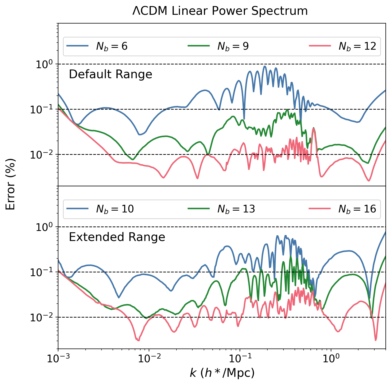
Figure 1: The $99.7$th percentile of the absolute errors on the $\Lambda$CDM linear power spectrum as a function of scale for several choices of number of basis functions used. The upper panel corresponds to the default range, while the lower panel corresponds to the extended range (see Table 1). Dashed lines indicate $0.01\%\,,0.1\%$ and $1\%$ errors, respectively.

III.2 Generalized Cosmologies: Curvature, Neutrinos and Dynamical Dark Energy

We now illustrate the power and generality of our approach by extending the treatment of the $\Lambda$CDM power spectrum to a much larger space of cosmological parameters. Specifically, we vary the neutrino mass $M_{\nu}$ while also considering the CPL dynamical dark energy parametrization $w(a)=w_{0}+w_{a}(1-a)$ [53, 54] and nonzero curvature. The weights $w_{i}(\Theta)$ now depend on nine rather than just three parameters. While we no longer benefit from the separability of Eq. (12) and strictly speaking all parameters except $A_{s}$ affect the shape of the power spectrum, some of them still do so only mildly. It suffices to fix $A_{s},h,z$ and $w_{a}$ for the purposes of constructing the templates, so that any change in the shape due to variations in the parameters can simply be absorbed into the weight functions. The associated ranges and grid sizes are indicated in Table 2. We emphasize again that the templates do not need to be computed exactly, and we need at most $\sim 80\,000$ calls to CAMB for the SVD . For the extended range, we use the parameter $w_{+}=w_{0}+w_{a}$ rather than $w_{a}$ itself. Note that we need $w_{+}<0$ in order to enforce a period of early matter domination. With the possible exception of time-varying dark energy, the extended parameter ranges are broad and uninformative for Stage IV galaxy surveys [58, 59, 60].

	Default		Extended
$\Theta$	Range	Grid size	Range	Grid size
$\omega_{c}$	[0.095,0.145]	20	[0.082,0.153]	30
$\omega_{b}$	[0.0202,0.0238]	12	[0.020,0.025]	12
$\Omega_{K}$	[-0.12,0.12]	12	[-0.2,0.2]	12
$h$	[0.55,0.8]	$h^{*}=0.7$	[0.51,0.89]	$h^{*}=0.7$
$n_{s}$	[0.9,1.02]	8	[0.81,1.09]	15
$M_{\nu}$ [eV]	[0,0.6]	12	[0,0.95]	15
$w_{0}$	[-1.25,-0.75]	12	[-1.38,-0.62]	15
$w_{a}/w_{+}$	[-0.3,0.3]	$w_{a}^{*}=0$	[-1.78,-0.42]	$w_{+}^{*}=-1$
$z$	[0.1,3]	$z^{*}=0$	[0.1,3]	$z^{*}=0$
$10^{9}A_{s}$	-	$10^{9}A_{s}^{*}=2$	-	$10^{9}A_{s}^{*}=2$

Table 2: Ranges and template grids for the generalized cosmological parameter space. If a parameter is held fixed for the templates, its fiducial value is indicated instead. The templates are always linearly spaced across the indicated range.The volume of the extended space is roughly $\sim 65$ times larger than that of the default space.

Extracting the first $30$ components takes $\mathcal{O}(10)$ min on a single CPU (but requires significant memory if the number of templates is large), while determining the coefficients of the RBF approximation of the weights takes negligible time. We use $N_{n}=20\,000$ Halton nodes across the $9$-dimensional parameter space. As for the $\Lambda$CDM power spectrum, we again found it beneficial to normalize the weights before applying the RBF. Details are given in Appendix C. We use $\sim 20\,000$ randomly selected cosmologies to test the precision of the predictions.

The precision of the resulting linear power spectrum decomposition is shown in Figure 2. We are again able to reach below $0.1\%$ precision for $99.7\%$ of the test samples for the default range and below $0.2\%$ for the extended range. This increase is due to inaccuracies in the RBF approximation, which is not surprising given that we have used the same number of Halton nodes for both the default and the extended parameter ranges. Appendix C contains further details on how we partially mitigated these inaccuracies. Increasing the number of Halton nodes will likely ameliorate this issue, but we did not pursue this any further. Importantly, the dashed curves in the bottom panel of Figure 2 illustrate that the accuracy of the decomposition from Eq. (1) is still satisfactory - using e.g. $N_{b}=19$ would decrease the error further to $\sim 0.05\%$ across all scales. Calculating a single power spectrum takes $\sim 1$ ms, while calculating $250$ predictions takes $\sim 30$ ms. The speed-up from vectorization is less pronounced due to the fact that larger intermediate arrays need to be created compared to the linear power spectrum.

IV One-Loop Power Spectrum in Redshift Space

Using the decomposition of the linear power spectrum from Section III, the calculation of higher-order statistics or corrections to N-point functions is straightforward, as outlined in Section II. We illustrate this using the one-loop power spectrum of galaxies in redshift space for a $\Lambda$CDM cosmology, but emphasize that this choice is irrelevant - the calculation of higher N-point functions reduces to a one-time computation of a limited number of integrals which can be done using any method at hand, regardless of whether analytical techniques are available.

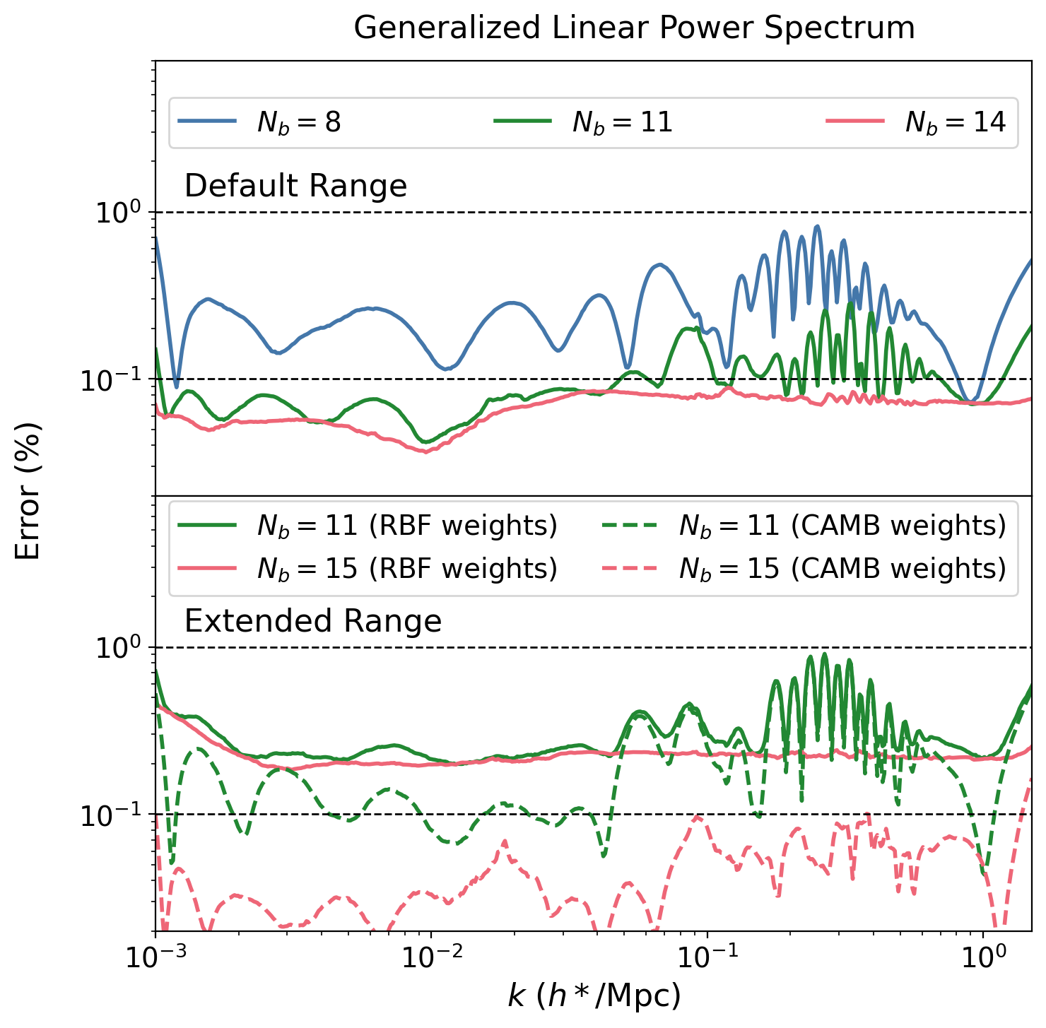
Figure 2: The $99.7$th percentile of the absolute errors on the generalized linear power spectrum as a function of scale for several choices of number of basis functions used. The upper panel corresponds to the default range, while the lower panel corresponds to the extended range. Dashed black lines indicate $0.01\%,\,0.1\%$ and $1\%$ errors, respectively. Dashed curves indicate the error if the weights are calculated exactly (i.e. using CAMB and Eq. (3)), while solid lines indicate the error if they are calculated using RBFs as detailed in Appendix C.

To test the precision of COBRA, we compare against the resummed EPT expression as implemented in the velocileptors code [37]. For the complete implementation of their model and all relevant expressions, we refer to their Appendix A and the velocileptors GitHub repository . All of the terms in this one-loop model are either constant, linear or quadratic functions of $P_{L}^{\Theta}$ (cf. Eq. 8), so that by Eq. (9) they reduce to matrix multiplications of size $N_{b}$ when Eq. (1) is substituted for the linear power spectrum. We choose to compute the entries of these matrices using FFTs via the implementation of [37]. We employ the same decomposition and parameter ranges as in Section III.1. We apply a Gaussian damping factor to the scale functions $v_{i}(k)$ to extrapolate beyond $k=4h^{*}$/Mpc, and a power law at low $k$. Since we now need to compute each of the loop integrals only once, we are free to choose a fairly large number of frequencies of $N_{f}=10\,000$. The IR resummation prescription we employ is detailed in Appendix B. We keep values of all four operator bias parameters fixed to the values listed in the velocileptors GitHub repository example notebook. Furthermore, we fix $A_{s}=2\times 10^{-9}$ and put all coefficients of terms $\propto k^{2}\mu^{2n}P_{L,\text{IR}}(k)$ equal to $40\,(50)$ in the default (extended) case and all coefficients of terms $\propto k^{2}\mu^{2n}$ to $3\,000$ . The $k\to 0$ contributions are subtracted from all loops to recover linear theory on large scales. We also employ RBF approximations for the $\Lambda$CDM growth rate and the velocity dispersion (see again Appendix B), but their impact on the total errors is small. We omit Alcock-Paczynski distortions, but these can be included at negligible additional cost since COBRA computes the full anisotropic power spectrum.

Figure 3 displays the error in calculating the monopole, quadrupole and hexadecapole using COBRA versus the truth using velocileptors on the range $10^{-3}h^{*}/\text{Mpc}<k<0.5h^{*}/\text{Mpc}$, using the same set of test functions as for the linear power spectrum.

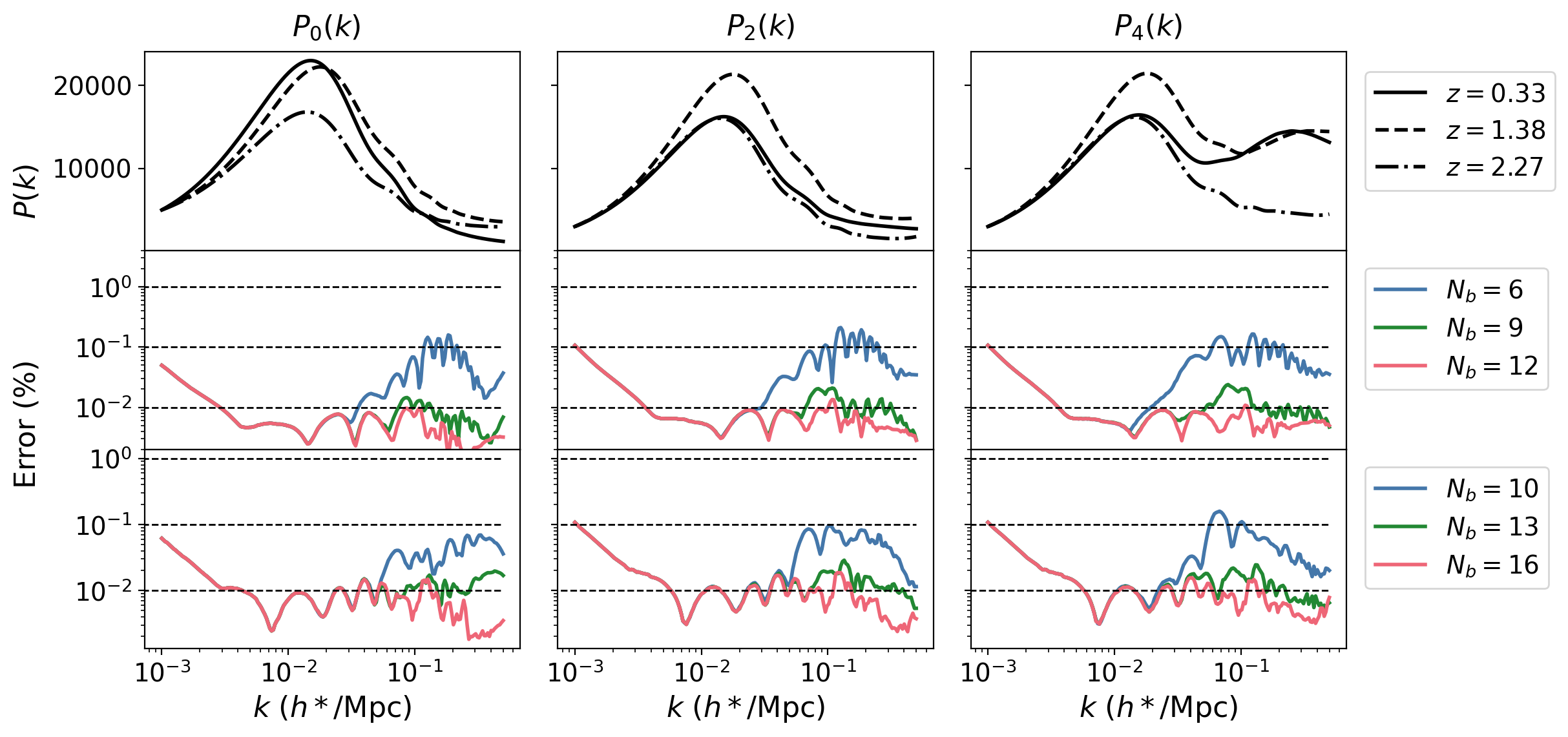
Figure 3: Performance of COBRA when applied to the IR-resummed one-loop power spectrum of galaxies in redshift space. Each column indicates a multipole, viz. monopole, quadrupole and hexadecapole from left to right. The top row displays three randomly selected cosmologies (solid, dashed and dot-dashed lines), while the second and third rows show the $99.7$th percentile of the errors on the test set (which matches the one used for the linear power spectra) as a function of scale for the default and extended parameter ranges, with the same choices of $N_{b}$ as in Figure 1. For visualization purposes, spectra are normalized to have the same overall amplitude.

In practice, the IR resummation procedure further reduces the error around the BAO scale compared to Figure 1 since wiggles are damped by an exponential factor with a known cosmology dependence. This is an immediate consequence of COBRA taking full advantage of the analytic structure of the loop corrections (see Appendix B), while direct emulation of the one-loop galaxy power spectrum (i.e. the individual terms multiplying bias coefficients) necessarily increases the number of cosmology dependent basis coefficients and thus constitutes a suboptimal expansion. As such, this approach could suffer from unnecessary accuracy losses compared to the linear theory prediction. For the default (extended) range, with $N_{b}=9\,(13)$ scale functions we can reach a precision of $\sim 0.01\%$ for $99.7\%$ of all test cosmologies in all multipoles. If we use a total of $12\,(16)$ components and $200$ wavenumber bins for the one-loop prediction, the resulting set of matrices required for all the different bias terms is around $25\,(40)$ MB in size. A single prediction takes $\sim 2.5$ ms, while $250$ predictions take roughly $65$ ms. Thus, with COBRA we are able to execute $\sim 4\,000$ model evaluations per second.

V Discussion

We have introduced COBRA, a method devised for efficient computation of large-scale structure observables, and applied it to the linear matter power spectrum and the one-loop power spectrum of galaxies in redshift space. Generalising our line of reasoning from Section II (and ignoring IR resummation for the sake of exposition, see Appendix B), all polyspectra $\mathcal{P}$ in perturbative approaches to LSS can be written as [10, 11]

$$\mathcal{P}^{\Theta}_{\ell\text{-loop}} = \text{const.}+\mathcal{S}^{l}[P_{L}^{\Theta}]$$

$$+ \mathcal{S}^{q}[P^{\Theta}_{L},P^{\Theta}_{L}]+\mathcal{S}^{c}[P^{\Theta}_{L},P^{\Theta}_{L},P^{\Theta}_{L}]$$

$$+ \dots$$

where $\mathcal{S}^{l},\mathcal{S}^{q}$ and $\mathcal{S}^{c}$ are linear, quadratic and cubic operators in terms of the linear power spectrum, and so on. Due to Wick’s theorem, all these operators are symmetric in their arguments, even in the case of cross-correlations of different tracers. Indeed, the cross-correlation of different tracers only affects the functional correlator dependence via different combinations of bias coefficients. Using our decomposition, given in Eq. (1), we obtain

$$\mathcal{P}^{\Theta}_{\ell\text{-loop}} = \text{const.}+\mathcal{S}_{i}^{l}w_{i}(\Theta)$$ (14)

$$+ \mathcal{S}_{ij}^{q}w_{i}(\Theta)w_{j}(\Theta)+\mathcal{S}_{ijk}^{c}w_{i}(\Theta)w_{j}(\Theta)w_{k}(\Theta)$$

$$+ \dots$$

with $\mathcal{S}_{i}^{l}=\mathcal{S}^{l}[v_{i}],\mathcal{S}_{ij}^{q}=\mathcal{S}^{q}[v_{i},v_{j}]$ and $\mathcal{S}_{ijk}^{c}=\mathcal{S}^{c}[v_{i},v_{j},v_{k}]$ cosmology-independent symmetric tensors. Thus, for the $d$-th order term in Eq. (V) (with $d$ arguments of $P_{L}$), the total number of tensor elements that need to be computed in a given wavenumber bin is

$$(\#\text{ of bias terms})\times{N_{b}+d-1\choose d}.$$ (15)

This provides a direct estimate of the memory requirements necessary for storing all tensors from Eq. (14). However, the number of individual integrals that need to be precomputed is much smaller; many terms contain factors of $P_{L}$ outside of the loop integral. For the one-loop bispectrum, the computationally most demanding contribution comes from the triangle diagram $B_{222}$, which integrates over all three linear power spectra. Naïve counting with $N_{b}=6$ and $15$ bias terms yields a total of $\sim 1\,000$ integrals to be evaluated across a specified set of wavenumber bins, which is certainly quite modest and much more efficient compared to the traditionally employed methods, e.g. FFTLog [10, 63]. Moreover, due to the decreasing ordering of singular values in SVD employed in COBRA (see Appendix B), we can expect that the number of basis functions necessary for reaching a given precision can be further reduced in terms that involve products of linear power spectra. Furthermore, integrated quantities (like mode coupling terms) might benefit from the additional reduction of a number of terms without compromising the precision compared to the linear power spectrum (see e.g. [11] for related findings in the bispectrum case). It may also be possible to reduce the number of required precomputations by using other compression methods [24]. Precision requirements could also loosen substantially when a realistic data covariance is taken into account [19, 63]. Given the small number of basis functions needed in our case, there is ample opportunity to generalise the calculations presented here to more realistic scenarios such as an exact treatment of time dependence [47, 64, 65], scenarios with scale-dependent growth [66] or higher-order N-point functions [67, 68, 22, 69, 70, 71, 72, 73, 74, 75, 76, 77].

To summarize, our work illustrates several key properties of COBRA; specifically, COBRA is:

fast:

The calculation for the linear power spectra can be done in $\sim 1$ ms on a single thread, while the loop calculation takes $\sim 2$ ms. Furthermore, all implementations are vectorized, which leads to further speed-ups when computing a few hundred predictions simultaneously without invoking additional computational resources such as GPU’s or TPU’s. This can be exploited when interfacing COBRA with samplers that admit vectorized likelihood evaluation such as UltraNest [78].

precise:

It is possible to reach $\sim 0.1\%$ precision on all observables considered here, and even better in the $\Lambda$CDM scenario. Thus, in performing cosmological inference one can comfortably ignore any numerical systematics due to miscalculating predictions of a given model. The precision of the output can be adjusted either through earlier truncation of the RBF-QR regression method or by including a smaller number of scale-dependent basis functions (using lower $N_{b}$). This is useful if further speed-up is desired and, moreover, does not require recalculating the tensors in Eq. (14).

general:

Once the linear power spectrum is decomposed into weights and scale functions, the cosmology dependence of nonlinear corrections is fully encoded in the weights. Computing them requires relatively modest resources and accuracy is not degraded, even for the large numbers of cosmological parameters that can be simultaneously constrained with Stage IV surveys. Analytical tools for calculating loop corrections are not required.

lightweight:

The tabulated scale functions require negligible memory, as do the coefficients of the polynomials needed to calculate the weights and the tensors for the one-loop power spectrum in redshift space. The implementation will be made publically available to download upon acceptance and requires only numpy and scipy.

We believe that the results of this work merit further exploration of several aspects. In particular, it would be interesting to explicitly consider the calculation of higher N-point functions such as the one-loop bispectrum and two-loop power spectrum with COBRA - we stress that the improvements over existing methods will be even more pronounced in this case. The very small number of coefficients used to approximate the linear power spectrum also facilitates a direct reconstruction, (see for example [79, 80, 81] for related work). In addition, other cosmology-independent and linear operations on observables, such as window convolution [82] or optimal signal-to-noise compression schemes [24], could also be incorporated in COBRA as a one-time calculation at the level of scale functions. Moreover, one could explore the accuracy of analytic derivatives of the RBF approximations to the scale functions in the context of a Fisher analysis or gradient-based sampling methods [83]. Finally, while the focus of this work, both in terms of scales and cosmological parameter ranges, has been on 3D observables relevant to galaxy clustering on large scales, it would be equally valuable to extend the treatment presented here to sky-projected (see, e.g. [84, 85] for some recent developments) or nonlinear quantities. These are more relevant for weak lensing and CMB probes.

Appendix A RBF-QR Regression

In the limit of small shape parameter $\epsilon$, the interpolation matrix $\Phi_{ab}^{\epsilon}$ from Eq. (5) becomes ill-conditioned. In this limit, the basis functions $\phi^{\epsilon}_{b}$ become increasingly flat. The columns of the interpolation matrix are nearly collinear, leading to numerical instabilities when computing the coefficients $f_{b}^{\epsilon}$. Additionally, large cancellations occur when computing the interpolant via Eq. (6). However, the resulting interpolant depends smoothly on the parameter $\epsilon$ (see e.g. [86, 32, 34, 35] and references therein). In other words, it is possible to construct the desired interpolant in a numerically stable way, just not by naïvely applying the two ill-conditioned steps of computing the coefficients $f_{b}^{\epsilon}$ and the sum in Eq. (6) in succession. Instead, the authors of [33] outline a simple way of avoiding these issues by transforming the interpolation problem Eq. (5) into a better-conditioned regression problem and this is the approach we implement. One can construct it in the following manner (we reproduce the results from [33], focusing initially on the one-variable case): first, one considers a truncated Mercer expansion of the form

$$e^{-\epsilon^{2}(\theta-\theta^{\prime})^{2}}\approx\sum_{k=1}^{M}\lambda_{k}^{\epsilon}\varphi_{k}^{\epsilon}(\theta)\varphi_{k}^{\epsilon}(\theta^{\prime})$$ (16)

where the basis functions $\varphi_{k}^{\epsilon}(\theta)$ (not to be confused with the $\phi_{a}(\Theta)$ from the main text) are given by

$$\varphi_{k}^{\epsilon}(\theta)=\sqrt{\frac{\beta}{2^{k-1}(k-1)!}}e^{-\delta^{2}\theta^{2}}H_{k-1}(\alpha\beta\theta)$$ (17)

with $\alpha$ a free hyperparameter, $\beta^{2}=\sqrt{1+(2\epsilon/\alpha)^{2}}$ and $\delta^{2}=\alpha^{2}(\beta^{2}-1)/2$ where $H_{k-1}$ is a (classical) Hermite polynomial;

$$H_{k}(x)=(-1)^{k}e^{x^{2}}\frac{\mathrm{d}^{k}}{\mathrm{d}x^{k}}e^{-x^{2}}.$$ (18)

The sequence $\lambda_{k}^{\epsilon}$ is exponentially decaying and given by

$$\lambda_{k}^{\epsilon}=\sqrt{\frac{\alpha^{2}}{\alpha^{2}+\epsilon^{2}+\delta^{2}}}\bigg{(}\frac{\epsilon^{2}}{\alpha^{2}+\epsilon^{2}+\delta^{2}}\bigg{)}^{k-1}.$$ (19)

The $\varphi_{k}^{\epsilon}(\theta)$ are orthonormal on the real axis with respect to a Gaussian weight function:

$$\int_{-\infty}^{\infty}\mathrm{d}\theta\frac{\alpha}{\sqrt{\pi}}e^{-\alpha^{2}\theta^{2}}\varphi_{k}^{\epsilon}(\theta)\varphi_{k^{\prime}}^{\epsilon}(\theta)=\delta_{kk^{\prime}};$$ (20)

by virtue of the standard orthogonality property of the Hermite polynomials . This identity shows that $\alpha$ controls the scale over which the functions $\varphi_{k}^{\epsilon}$ are supported. When $M\to\infty$, the right-hand side of Eq. (16) converges to the left-hand side. However, truncating the expansion at a suitably chosen value of $M$ allows the interpolation matrix to be written in the ‘low rank’ form

$$\Phi^{\epsilon}\approx(\tilde{\Phi}^{\epsilon})\Lambda^{\epsilon}(\tilde{\Phi}^{\epsilon})^{T}$$ (21)

where $\Lambda^{\epsilon}$ is an $M\times M$ diagonal matrix with $\lambda_{k}^{\epsilon}$ on the diagonal and the matrix $\tilde{\Phi}^{\epsilon}$ is $N_{n}\times M$, i.e. ‘slim’, since $M<N_{n}$ in practice, with entries $\tilde{\Phi}_{ak}^{\epsilon}=\varphi_{k}^{\epsilon}(\theta_{a})$. Early truncation of the expansion from Eq. (16) has the effect of making the calculation more stable. If the value of $\alpha$ is chosen suitably, the matrix $\tilde{\Phi}^{\epsilon}$ is much better conditioned than $\Phi^{\epsilon}$. It admits a pseudo-inverse $(\tilde{\Phi}^{\epsilon})^{\dagger}$ which can be computed via QR-decomposition without catastrophic loss of precision. By rewriting the computation of the interpolant $g(\theta)$ in terms of the $\varphi_{k}^{\epsilon}$ basis functions using Eq. (16), one can show that [33]

$$g(\theta)=\varphi_{k}^{\epsilon}(\theta)b_{k}^{\epsilon}$$ (22)

with $b_{k}^{\epsilon}=(\tilde{\Phi}^{\epsilon})_{ka}^{\dagger}g(\theta_{a})$, i.e. a simple dot product where $b_{k}^{\epsilon}$ can be precomputed because the vector $g(\theta_{a})$ is known by definition (it is computed at the nodes). The exact interpolation problem is replaced by an approximate regression for determining the $M$ unknown coefficients $b_{k}^{\epsilon}$ . Notably, the computation of Eq. (22) does not involve the matrix $\Lambda^{\epsilon}$ containing the small eigenvalues at any point, to which the authors of [33] attribute its numerical stability. This procedure was then dubbed RBF-QR regression, with QR referring to the QR decomposition of $\tilde{\Phi}^{\epsilon}$ and regression to the $M$-term truncation of Eq. (16), which leads to an overdetermined system of equations for the coefficients $b_{k}^{\epsilon}$ since $M<N_{n}$.

In the $D$-variable case (keeping $\epsilon$ the same for all dimensions) we can write the exponential of the sum as a product of exponentials, so that Eq. (16) is generalized to

$$e^{-\epsilon^{2}(\Theta-\Theta^{\prime})_{m}(\Theta-\Theta^{\prime})_{m}}\approx\sum_{\mathbf{k}=\mathbf{1}_{D}}^{\mathbf{M}}\lambda_{\mathbf{k}}^{\epsilon}\varphi_{\mathbf{k}}^{\epsilon}(\Theta)\varphi_{\mathbf{k}}^{\epsilon}(\Theta^{\prime})$$ (23)

where we use multi-index notation, i.e. $\mathbf{1}_{D}=(1,1,\dots 1)$ while $\mathbf{k}=(k_{1},k_{2},\dots k_{D})$ and

$$\varphi_{\mathbf{k}}^{\epsilon}(\Theta)=\prod_{m=1}^{D}\varphi_{k_{m}}^{\epsilon}(\Theta_{m}).$$ (24)

The size of the eigenvalues is dictated by the sum $S_{m}=k_{1}+\dots+k_{m}$ of the indices:

$$\lambda_{\mathbf{k}}^{\epsilon}=\bigg{(}\frac{\alpha^{2}}{\alpha^{2}+\epsilon^{2}+\delta^{2}}\bigg{)}^{D/2}\bigg{(}\frac{\epsilon^{2}}{\alpha^{2}+\epsilon^{2}+\delta^{2}}\bigg{)}^{S_{m}-D}.$$ (25)

For this reason, it is natural to truncate Eq. (23) at some value $S_{\text{max}}$ of $S_{m}$, thus keeping all terms with index sum at most $S_{\text{max}}$. From Eq. (17), we infer that this corresponds to keeping all polynomials in the (rescaled) $\Theta_{m}$ variables of total degree $S_{\text{max}}-D$, of which there are $M={S_{\text{max}}\choose D}$. Thus, from now on, $M$ again refers to the total number of terms kept in the sum.

The expression from Eq. (22) is not ill-conditioned when $\epsilon$ is small, provided the parameters $M$ and $\alpha$ are chosen carefully. If $M$ is too small, the expansion from Eq. (16) is not converged; if it is too large then the regression problem for determining $h_{k}^{\epsilon}$ is still ill-conditioned. If $\alpha$ is too small, the basis functions $\varphi_{k}^{\epsilon}$ are too broad and vice versa. We found that $\epsilon=0.1$ with $\alpha$ between $1.8$ and $2.5$ and $M\sim N_{n}/4$ to yield satisfactory results in all dimensions. Furthermore, we have checked that adding some fraction of noise ($\sim 10^{-5}$, thus below the accuracy levels of the interpolant) to the input weights computed at the Halton nodes leads to completely negligible differences in the resulting interpolant.

Appendix B IR Resummation

The observed galaxy power spectrum exhibits baryon acoustic oscillations with a smaller amplitude than the expectation from linear theory. This feature can be consistently taken into account via IR resummation. In Eulerian space, this is typically done by adopting a wiggle-no-wiggle split of the linear power spectrum. The no-wiggle part $P_{\text{nw}}$ is constructed by applying a suitable smoothing operation $\mathcal{F}$ to the linear power spectrum [89, 90, 91]:

$$P_{\text{nw}}^{\Theta}(k)=\mathcal{F}[P^{\Theta}_{L}](k).$$ (26)

The IR-resummed power spectrum at the linear level in redshift space is then given by [89, 90, 92, 91]

$$P^{\Theta}_{L,\text{IR}}(k,\mu) = P_{\text{nw}}^{\Theta}(k)+e^{-k^{2}\Sigma_{s}^{2}(\Theta,\mu)}(P^{\Theta}_{L}(k)-P_{\text{nw}}^{\Theta}(k))$$ (27)

$$= P_{\text{nw}}^{\Theta}(k)+e^{-k^{2}\Sigma_{s}^{2}(\Theta,\mu)}P_{\text{w}}^{\Theta}(k),$$

with the redshift-space damping factor,

$$\Sigma_{s}^{2}(\Theta,\mu)=(1+f(\Theta)(f(\Theta)+2)\mu^{2})\Sigma^{2}(\Theta),$$ (28)

and the isotropic real-space damping,

$$\Sigma^{2}(\Theta)=\int_{0}^{k_{\text{o}}}\frac{\mathrm{d}q}{6\pi^{2}}(1-j_{0}(qr_{\text{o}})+2j_{2}(qr_{\text{o}})P_{\text{nw}}(q).$$ (29)

We use $r_{o}=105\text{ Mpc}/h^{*}$ and $k_{o}=0.2h^{*}/\text{Mpc}$, independently of cosmology. At one-loop order the power spectrum becomes [92, 91]

$$P^{\Theta}_{\text{1-loop,IR}}(k,\mu) = \text{const.}+\mathcal{S}^{l}[P^{\Theta}_{\text{nw}}]$$ (30)

$$+ e^{-k^{2}\Sigma_{s}^{2}}(1+k^{2}\Sigma_{s}^{2})\mathcal{S}^{l}[P^{\Theta}_{\text{w}}]$$

$$+ \mathcal{S}^{q}[P^{\Theta}_{L,\text{IR}},P^{\Theta}_{L,\text{IR}}]$$

where we suppressed some arguments to avoid clutter and $\mathcal{S}^{l},\mathcal{S}^{q}$ are as in Eq. (8). The last line of Eq. (30) depends on cosmology not only via the linear power spectrum, but also through the damping factor in the exponential from Eq. (28). A commonly used form is to write the quadratic term as [89, 90, 91, 14]

$$\mathcal{S}^{q}[P^{\Theta}_{L,\text{IR}},P^{\Theta}_{L,\text{IR}}] \approx \mathcal{S}^{q}[P^{\Theta}_{\text{nw}},P^{\Theta}_{\text{nw}}]$$

$$+ e^{-k^{2}\Sigma_{s}^{2}}\bigg{(}\mathcal{S}^{q}[P^{\Theta}_{L},P^{\Theta}_{L}]-\mathcal{S}^{q}[P^{\Theta}_{\text{nw}},P^{\Theta}_{\text{nw}}]\bigg{)}.$$

Various methods have been proposed in the literature to accomplish the smoothing in Eq. (26) [89, 90, 93, 94]. We would like the decomposition of Eq. (1) to translate immediately into a decomposition of the wiggle and no-wiggle parts of a given power spectrum. The straightforward way to achieve this is by choosing a smoothing operation that is linear, i.e. $\mathcal{F}[\lambda P]=\lambda\mathcal{F}[P]$ and $\mathcal{F}[P_{1}+P_{2}]=\mathcal{F}[P_{1}]+\mathcal{F}[P_{2}]$. Then, provided that we have a satisfactory approximation of the linear power spectrum, we can assert that

$$P_{\text{nw}}^{\Theta}(k) = \mathcal{F}[w_{i}(\Theta)v_{i}](k)=w_{i}(\Theta)\mathcal{F}[v_{i}](k)$$ (32)

$$= w_{i}(\Theta)v_{i}^{\text{nw}}(k),$$

and correspondingly

$$P_{\text{w}}^{\Theta}(k) = w_{i}(\Theta)(v_{i}(k)-\mathcal{F}[v_{i}](k))$$ (33)

$$= w_{i}(\Theta)v_{i}^{\text{w}}(k).$$

In other words, if the filter $\mathcal{F}$ is linear, the scale functions $v_{i}(k)$ for the linear power spectrum can be smoothed individually to yield appropriate bases $v_{i}^{\text{w}}(k)$ and $v_{i}^{\text{nw}}(k)$ for the wiggle and no-wiggle parts, respectively. If the filter were explicitly cosmology dependent, then the separation of the cosmology dependence and scale dependence would no longer be realized already at the linear level. Hence, we need to choose a filter that is also not cosmology dependent. To this end, we employ the Gaussian 1D filter in logarithmic wavenumbers from [90], after normalizing the linear power spectrum by the Eisenstein-Hu power spectrum $P^{*}_{\text{EH}}(k)$ [95] at a fixed cosmology:

$$P^{\Theta}_{\text{nw}}(k) = P^{*}_{\text{EH}}(k)\frac{1}{\lambda(k)\sqrt{2\pi}}\int\mathrm{d}\log{q}\frac{P^{\Theta}_{L}(10^{\log{q}})}{P^{*}_{\text{EH}}(10^{\log{q}})}$$ (34)

$$\times \exp{\bigg{(}-\frac{1}{2\lambda(k)^{2}}(\log{q}-\log{k})^{2}\bigg{)}}.$$

Here it is important to introduce a scale dependence in $\lambda$ so that it becomes small at both high and low $k$. This is done in order to make sure that the cut-offs introduced when computing the loop integrals (cf. Section IV) do not spoil the agreement between $P_{\text{nw}}(k)$ and $P_{L}(k)$ at high and low values of $k$. The result of applying the filter to the scale functions is shown in Figure 4. For $i=1$, the scale function has essentially the same shape as the linear power spectrum and exhibits no zero crossings. However, the higher scale functions have more and more features. It is not at all clear from intuition what the smoothed version of all but the lowest few scale functions should look like; however, by virtue of the linearity of the filter we are able to ensure that no spurious features are introduced.

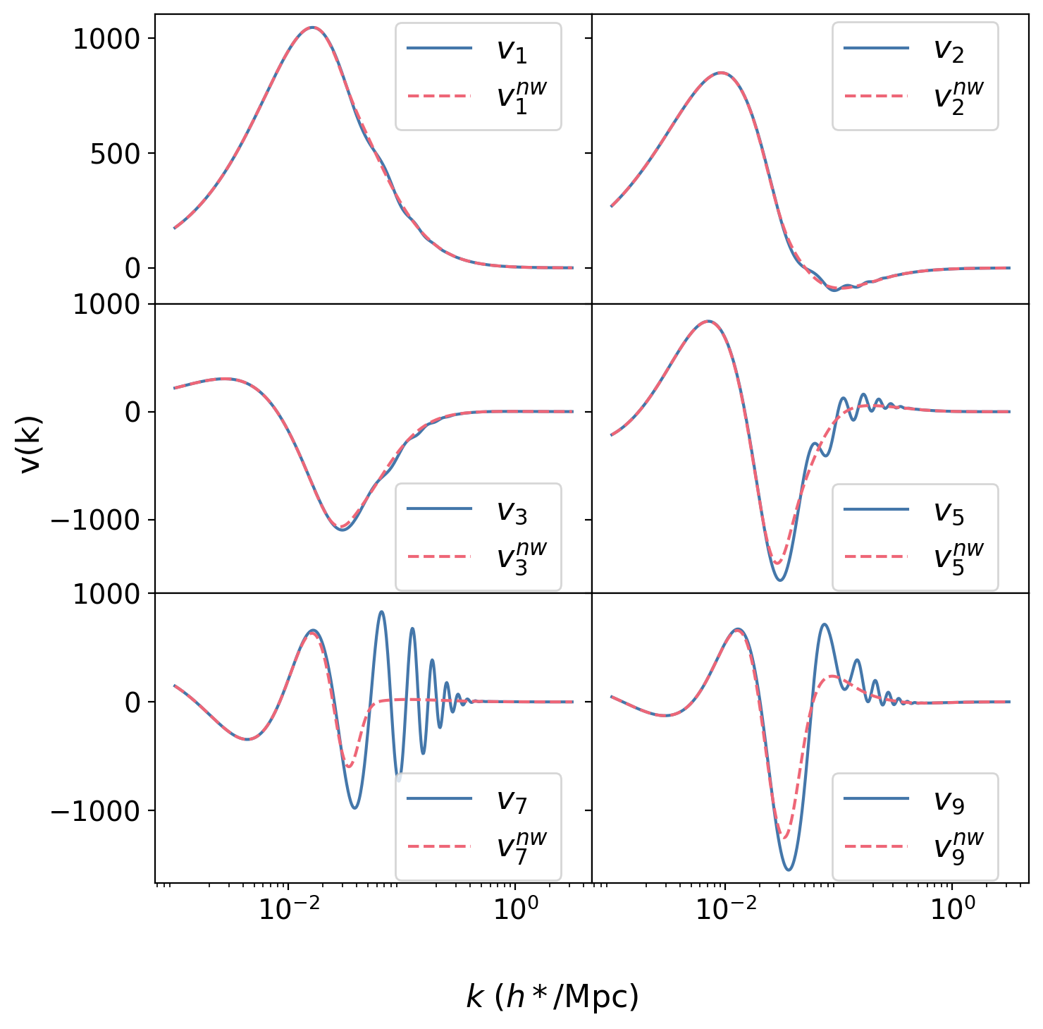
Figure 4: Some examples of scale functions $v_{i}(k)$(solid blue) along with their no-wiggle counterparts $v_{i}^{\text{nw}}(k)$ (dashed pink) obtained by applying Eq. (34). These correspond to the basis for the extended $\Lambda$CDM settings.

The amplitude of the no-wiggle scale functions stays roughly the same, while the associated singular values (taken as a measure for the associated weights) decay quickly, as shown in Figure 5. Consequently, Eq. (32) becomes accurate very quickly. Interestingly, however, the amplitude of the wiggly scale functions $v_{i}^{\text{w}}(k)$ clearly increases with the index $i$, so that the convergence of the wiggle part given in Eq. (33) is somewhat slower than the no-wiggle part. Thus, the higher scale functions contribute relatively little to the broadband power and mostly to $P_{\text{w}}(k)$. This is why the IR-resummed power spectrum is more easily approximated with a given number of scale functions than the original power spectrum, as observed in Section IV.

An alternative approach (which we did not pursue) would be to perform the wiggle-no-wiggle split for each cosmology from the start using any filter, and then perform the SVD for the wiggle and no-wiggle power spectra separately. The advantage of that approach might be that one does not need a linear filter. Given the discussion above, it is not clear which approach will provide a more optimal basis, and we leave this for future work.

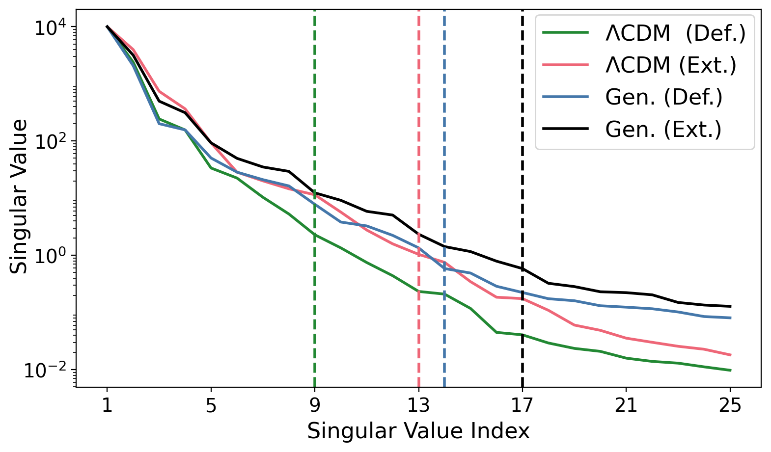
Figure 5: First 25 singular values of the SVD for all four parameter spaces considered in this work, arbitrarily normalized to have the same largest singular value. The horizontal lines indicate the number of basis functions needed to reach $\sim 0.1\%$ precision for $99.7\%$ of the test samples around $k=0.1h^{*}$/Mpc.

Finally, owing to Eq. (B) the separation of scale dependence and cosmology dependence is maintained also at the one-loop level. We have

$$P^{\Theta}_{\text{1-loop,IR}}(k,\mu) = \text{const.}+\mathcal{S}_{i}^{l,\text{nw}}w_{i}(\Theta)$$ (35)

$$+ e^{-k^{2}\Sigma_{s}^{2}}(1+k^{2}\Sigma_{s}^{2})\mathcal{S}_{i}^{l,\text{w}}w_{i}(\Theta)$$

$$+ \mathcal{S}_{ij}^{q,\text{nw}}w_{i}(\Theta)w_{j}(\Theta)$$

$$+ e^{-k^{2}\Sigma_{s}^{2}}\mathcal{S}_{ij}^{q,\text{w}}w_{i}(\Theta)w_{j}(\Theta)$$

where the linear pieces are $\mathcal{S}_{i}^{l,\text{nw}}=\mathcal{S}^{l}(v^{\text{nw}}_{i})$ and $\mathcal{S}_{i}^{l,\text{w}}=\mathcal{S}^{l}(v^{\text{w}}_{i})$ while the quadratic pieces are $\mathcal{S}_{ij}^{q,\text{nw}}=\mathcal{S}^{q}[v^{\text{nw}}_{i},v^{\text{nw}}_{j}]$ and $\mathcal{S}_{ij}^{q,\text{w}}=\mathcal{S}^{q}[v_{i},v_{j}]-\mathcal{S}^{q}[v^{\text{nw}}_{i},v^{\text{nw}}_{j}]$. This is what is used in Section IV. We approximate $\Sigma^{2}$ in a similar fashion as in Section III.1 and the growth rate by first normalizing by the analytic solution for $\Omega_{m}+\Omega_{\Lambda}=1$.

Regarding the extensions of the IR resummation to the higher N-point functions, an analogous expression to the one given in Eq. (30) has also been derived for bispectrum [91], which can be recast into a form analogous to Eq. (B) without loss of accuracy. As with the power spectrum, this latter form is particularly convenient for implementation in the COBRA framework. Recently, an alternative derivation of the bispectrum IR-resummation was presented in [96], where a comprehensive resummation of long displacement fields was performed, including the derivation of IR suppression in the wiggle part. These results also demonstrate how IR resummation can be applied to higher N-point functions, ultimately leading to a similarly convenient wiggle-no-wiggle form. In conclusion, the COBRA framework is well-suited for the implementation of the IR resummation via the wiggle no-wiggle approximations even in higher N-point functions.

Appendix C Weights for Generalized Cosmologies

For the decomposition of the linear matter power spectrum including dynamical dark energy, massive neutrinos and curvature as presented in Section III.2, we found it beneficial to factor the calculation of the weights as

$$w_{i}(\Theta)=\frac{w_{i}(\Theta)}{\sqrt{P_{L}^{\Theta}(k_{1})P_{L}^{\Theta}(k_{2})}}\frac{\sqrt{P_{L}^{\Theta}(k_{1})P_{L}^{\Theta}(k_{2})}}{D^{2}_{+}(\Theta)}D^{2}_{+}(\Theta)$$ (36)

where $D_{+}(\Theta)$ is the scale-independent growth factor in the corresponding cosmology without neutrinos, $k_{1}\approx 0.009h^{*}/$Mpc and $k_{2}\approx 0.47h^{*}/$Mpc. The two ratios in the above expression are rather slowly varying functions of cosmology and can hence be approximated accurately using our RBF method. Thus, after applying the RBF approximation to these ratios (which still depend nontrivially on all nine parameters) it remains to compute $D_{+}(\Theta)$, which depends on six parameters in total (i.e. the total physical cold matter density $\omega_{m}=\omega_{b}+\omega_{c}$ as well as $\Omega_{K},h,w_{0},w_{a}$ and $z$). Solving the ordinary differential equation that defines $D_{+}$ would be slow compared to the calculation of the RBF interpolant and the sum over scale functions, and there is no hope of making analytic progress in the case of a time-varying equation of state $w_{a}\neq 0$. Therefore we adopt a different procedure.

The growing mode in a universe with ordinary matter, cosmological constant and curvature can be expanded in $\Omega_{K}$ and is given (for positive $\Omega_{\Lambda}$ and $|\Omega_{K}/(1-\Omega_{K})|<1$) by the series [97]

$$\frac{D_{+}(\Theta)}{a} = R(a)\sum_{n=0}^{\infty}\frac{5(-1)^{n}(3/2)_{n}}{n!(5+2n)}\bigg{(}\frac{\Omega_{K}q^{1/3}}{\Omega_{m}^{2/3}\Omega_{\Lambda}^{1/3}(1+q)}\bigg{)}^{n}$$ (37)

$$\times {}_{2}F_{1}\left(1,\frac{1-2n}{3},\frac{11+2n}{6},-q\right)$$

where $q=\Omega_{\Lambda}a^{3}/\Omega_{m}$ and $R(a)=H(a)/H_{K=0}(a)$ is the ratio of the Hubble factor to its value when the curvature term is set to zero, i.e.

$$R^{2}(a)=\frac{\Omega_{m}a^{-3}+\Omega_{K}a^{-2}+\Omega_{\Lambda}}{\Omega_{m}a^{-3}+\Omega_{\Lambda}}.$$ (38)

Furthermore, there also exists an exact solution for the growing mode in cosmologies with zero curvature, but non-trivial (constant) equation of state $w_{0}$ [98]:

$$\frac{D_{+}(\Theta)}{a}={}_{2}F_{1}\left(\frac{w_{0}-1}{2w_{0}},\frac{-1}{3w_{0}},1-\frac{5}{6w_{0}},-q_{w}\right)$$ (39)

with $q_{w}=\Omega_{\Lambda}a^{-3w_{0}}/\Omega_{m}$. A solution in the case of non-vanishing curvature as well as non-trivial equation of state appears to be unknown, but we can instead make the following ansatz, denoted by an overbar to distinguish it from the true solution:

$$\frac{\bar{D}(\Theta)}{a} = R(a)\sum_{n=0}^{\infty}\frac{5(-1)^{n}(3/2)_{n}}{n!(5+2n)}\bigg{(}\frac{\Omega_{K}q_{w}^{1/3}}{\Omega_{m}^{2/3}\Omega_{\Lambda}^{1/3}(1+q_{w})}\bigg{)}^{n}$$ (40)

$$\times {}_{2}F_{1}\left(\frac{w_{0}-1}{2w_{0}},\frac{2n-1}{3w_{0}},1-\frac{5+2n}{6w_{0}},-q_{w}\right),$$

where now the time variable in the summation is

$$q_{w}=\frac{\Omega_{\Lambda}}{\Omega_{m}}a^{-3(w_{0}+w_{a})}\exp\big{(}3w_{a}(a-1)\big{)}$$ (41)

and the prefactor $R(a)$ is modified correspondingly by substituting [54]

$$\Omega_{\Lambda}\to\Omega_{\Lambda}a^{-3(1+w_{0}+w_{a})}\exp\big{(}3w_{a}(a-1)\big{)}$$ (42)

in Eq. (38). The expression in Eq. (40) is an amalgamation of Eq. (37),(39). By construction, $\bar{D}$ reduces to the above exact solutions in the limiting cases where $w_{a}=0$ and either $\Omega_{K}=0$ or $w_{0}=-1$, respectively. We decomposed the ratio of the exact growth factor by this quantity, while keeping the first $15$ terms in the series expansion (this can be computed at negligible cost). Thus, the weights are factorized as

$$w_{i}(\Theta) = \frac{w_{i}(\Theta)}{\sqrt{P_{L}^{\Theta}(k_{1})P_{L}^{\Theta}(k_{2})}}\frac{\sqrt{P_{L}^{\Theta}(k_{1})P_{L}^{\Theta}(k_{2})}}{D^{2}_{+}(\Theta)}$$ (43)

$$\times \frac{D^{2}_{+}(\Theta)}{\bar{D}^{2}(\Theta)}\bar{D}^{2}(\Theta).$$

Here, we use $15\,000$ Halton nodes in the six-dimensional parameter space corresponding to the third term in the above expression.

For the default parameter ranges from the left column Table 2, Eq. (43) was sufficient for our purposes as it achieves an accuracy of below $0.1\%$ for $99.7\%$ of the test cosmologies. However, for the extended parameter ranges from the right column of 2 it yielded an overall error just below $1\%$ on the test spectra, which we deemed unacceptable. We managed to mitigate this issue via the following two modifications: (i) instead of directly applying the RBF to the second factor in (43), we first applied a scaled logit transformation and then transformed back, and (ii) instead applying the RBF to $D^{2}_{+}(\Theta)/\bar{D}^{2}(\Theta)$ we applied it to $D^{2}_{+}(\Theta)/\bar{D}^{2\alpha}(\Theta)$ with $\alpha=0.35$. The result of this procedure is what is shown in the bottom panel of Figure 2 as the solid curves. These two modifications did not have any discernible impact on the results for the default range, so we did not apply them there. We emphasize again that there are many alternative procedures that could lead to similar or improved results for the calculation of the weights, but we leave these investigations as well as a thorough comparison to our RBF method for future work.

References

- Aghamousa et al. [2016] A. Aghamousa et al. (DESI), The DESI Experiment Part I: Science,Targeting, and Survey Design, (2016), arXiv:1611.00036 [astro-ph.IM] .
- Scaramella et al. [2022] R. Scaramella et al. (Euclid), Euclid preparation. I. The Euclid Wide Survey, Astron. Astrophys. 662, A112 (2022), arXiv:2108.01201 [astro-ph.CO] .
- LSST Dark Energy Science Collaboration [2012] LSST Dark Energy Science Collaboration, Large Synoptic Survey Telescope: Dark Energy Science Collaboration, arXiv e-prints , arXiv:1211.0310 (2012), arXiv:1211.0310 [astro-ph.CO] .
- Adame et al. [2024] A. G. Adame et al. (DESI), DESI 2024 VI: Cosmological Constraints from the Measurements of Baryon Acoustic Oscillations, (2024), arXiv:2404.03002 [astro-ph.CO] .
- Bernardeau et al. [2002] F. Bernardeau, S. Colombi, E. Gaztañaga, and R. Scoccimarro, Large-scale structure of the Universe and cosmological perturbation theory, Phys. Rep. 367, 1 (2002), arXiv:astro-ph/0112551 [astro-ph] .
- Desjacques et al. [2018] V. Desjacques, D. Jeong, and F. Schmidt, Large-scale galaxy bias, Phys. Rep. 733, 1 (2018), arXiv:1611.09787 [astro-ph.CO] .
- Carrasco et al. [2012] J. J. M. Carrasco, M. P. Hertzberg, and L. Senatore, The effective field theory of cosmological large scale structures, Journal of High Energy Physics 2012, 82 (2012), arXiv:1206.2926 [astro-ph.CO] .
- Baumann et al. [2012] D. Baumann, A. Nicolis, L. Senatore, and M. Zaldarriaga, Cosmological non-linearities as an effective fluid, J. Cosmology Astropart. Phys 2012, 051 (2012), arXiv:1004.2488 [astro-ph.CO] .
- Schmittfull and Vlah [2016] M. Schmittfull and Z. Vlah, Reducing the two-loop large-scale structure power spectrum to low-dimensional, radial integrals, Phys. Rev. D 94, 103530 (2016), arXiv:1609.00349 [astro-ph.CO] .
- Simonović et al. [2018] M. Simonović, T. Baldauf, M. Zaldarriaga, J. J. Carrasco, and J. A. Kollmeier, Cosmological perturbation theory using the FFTLog: formalism and connection to QFT loop integrals, Journal of Cosmology and Astropartictle Physics 2018, 030 (2018), arXiv:1708.08130 [astro-ph.CO] .
- Anastasiou et al. [2024] C. Anastasiou, D. P. L. Bragança, L. Senatore, and H. Zheng, Efficiently evaluating loop integrals in the EFTofLSS using QFT integrals with massive propagators, Journal of High Energy Physics 2024, 2 (2024), arXiv:2212.07421 [astro-ph.CO] .
- Schmittfull et al. [2016] M. Schmittfull, Z. Vlah, and P. McDonald, Fast large scale structure perturbation theory using one-dimensional fast Fourier transforms, Phys. Rev. D 93, 103528 (2016), arXiv:1603.04405 [astro-ph.CO] .
- Aricò et al. [2021] G. Aricò, R. E. Angulo, and M. Zennaro, Accelerating Large-Scale-Structure data analyses by emulating Boltzmann solvers and Lagrangian Perturbation Theory, arXiv e-prints , arXiv:2104.14568 (2021), arXiv:2104.14568 [astro-ph.CO] .
- Eggemeier et al. [2023] A. Eggemeier, B. Camacho-Quevedo, A. Pezzotta, M. Crocce, R. Scoccimarro, and A. G. Sánchez, COMET: Clustering observables modelled by emulated perturbation theory, MNRAS 519, 2962 (2023), arXiv:2208.01070 [astro-ph.CO] .
- DeRose et al. [2022] J. DeRose, S.-F. Chen, M. White, and N. Kokron, Neural network acceleration of large-scale structure theory calculations, J. Cosmology Astropart. Phys 2022, 056 (2022), arXiv:2112.05889 [astro-ph.CO] .
- Spurio Mancini et al. [2022] A. Spurio Mancini, D. Piras, J. Alsing, B. Joachimi, and M. P. Hobson, COSMOPOWER: emulating cosmological power spectra for accelerated Bayesian inference from next-generation surveys, MNRAS 511, 1771 (2022), arXiv:2106.03846 [astro-ph.CO] .
- Cataneo et al. [2017] M. Cataneo, S. Foreman, and L. Senatore, Efficient exploration of cosmology dependence in the EFT of LSS, J. Cosmology Astropart. Phys 2017, 026 (2017), arXiv:1606.03633 [astro-ph.CO] .
- Chen et al. [2021] S.-F. Chen, Z. Vlah, E. Castorina, and M. White, Redshift-space distortions in Lagrangian perturbation theory, J. Cosmology Astropart. Phys 2021, 100 (2021), arXiv:2012.04636 [astro-ph.CO] .
- Trusov et al. [2024] S. Trusov, P. Zarrouk, and S. Cole, Neural Network-based model of galaxy power spectrum: Fast full-shape galaxy power spectrum analysis, arXiv e-prints , arXiv:2403.20093 (2024), arXiv:2403.20093 [astro-ph.CO] .
- Ramirez et al. [2023] S. Ramirez, M. Icaza-Lizaola, S. Fromenteau, M. Vargas-Magaña, and A. Aviles, Full Shape Cosmology Analysis from BOSS in configuration space using Neural Network Acceleration, arXiv e-prints , arXiv:2310.17834 (2023), arXiv:2310.17834 [astro-ph.CO] .
- Philcox et al. [2022] O. H. E. Philcox, M. M. Ivanov, G. Cabass, M. Simonović, M. Zaldarriaga, and T. Nishimichi, Cosmology with the redshift-space galaxy bispectrum monopole at one-loop order, Phys. Rev. D 106, 043530 (2022), arXiv:2206.02800 [astro-ph.CO] .
- D’Amico et al. [2022a] G. D’Amico, Y. Donath, M. Lewandowski, L. Senatore, and P. Zhang, The BOSS bispectrum analysis at one loop from the Effective Field Theory of Large-Scale Structure, arXiv e-prints , arXiv:2206.08327 (2022a), arXiv:2206.08327 [astro-ph.CO] .
- Note [1] In order for Eq. (1) to remain satisfied, we can only apply linear and cosmology-independent transformations to the templates - other commonly used transformations such as taking logarithms or dividing by a cosmology-dependent fitting formula would spoil the decomposition. We also attempted whitening the templates, i.e. subtracting the mean and dividing by the standard deviation, but this resulted in significantly degraded performance.
- Philcox et al. [2021] O. H. E. Philcox, M. M. Ivanov, M. Zaldarriaga, M. Simonović, and M. Schmittfull, Fewer mocks and less noise: Reducing the dimensionality of cosmological observables with subspace projections, Phys. Rev. D 103, 043508 (2021), arXiv:2009.03311 [astro-ph.CO] .
- Pathak et al. [2024a] L. Pathak, A. Reza, and A. S. Sengupta, Fast and faithful interpolation of numerical relativity surrogate waveforms using meshfree approximation, arXiv e-prints , arXiv:2403.19162 (2024a), arXiv:2403.19162 [gr-qc] .
- Pathak et al. [2024b] L. Pathak, S. Munishwar, A. Reza, and A. S. Sengupta, Prompt sky localization of compact binary sources using a meshfree approximation, Phys. Rev. D 109, 024053 (2024b), arXiv:2309.07012 [gr-qc] .
- Halko et al. [2011] N. Halko, P. G. Martinsson, and J. A. Tropp, Finding structure with randomness: Probabilistic algorithms for constructing approximate matrix decompositions, SIAM Review 53, 217 (2011), https://doi.org/10.1137/090771806 .
- Eckart and Young [1936] C. Eckart and G. Young, The approximation of one matrix by another of lower rank, Psychometrika 1, 211–218 (1936).
- Buhmann [2003] M. D. Buhmann, Radial Basis Functions: Theory and Implementations, Cambridge Monographs on Applied and Computational Mathematics (Cambridge University Press, 2003).
- Owen [2017] A. B. Owen, A randomized halton algorithm in r (2017), arXiv:1706.02808 [stat.CO] .
- Note [2] Here and throughout, we will use isotropic Gaussians. It would certainly be interesting to consider generalizations with different (physically motivated) values of in different dimensions - this is mathematically straightforward [33] and could lead to improved performance with fewer nodes.
- Fornberg et al. [2011] B. Fornberg, E. Larsson, and N. Flyer, Stable computations with gaussian radial basis functions, SIAM J. Sci. Comput. 33, 869 (2011).
- Fasshauer and McCourt [2012] G. E. Fasshauer and M. J. McCourt, Stable evaluation of gaussian radial basis function interpolants, SIAM Journal on Scientific Computing 34, A737 (2012), https://doi.org/10.1137/110824784 .
- Fornberg and Piret [2008] B. Fornberg and C. Piret, A stable algorithm for flat radial basis functions on a sphere, SIAM Journal on Scientific Computing 30, 60 (2008), https://doi.org/10.1137/060671991 .
- Driscoll and Fornberg [2002] T. Driscoll and B. Fornberg, Interpolation in the limit of increasingly flat radial basis functions, Computers & Mathematics with Applications 43, 413 (2002).
- Senatore [2015] L. Senatore, Bias in the effective field theory of large scale structures, J. Cosmology Astropart. Phys 2015, 007 (2015), arXiv:1406.7843 [astro-ph.CO] .
- Chen et al. [2020] S.-F. Chen, Z. Vlah, and M. White, Consistent modeling of velocity statistics and redshift-space distortions in one-loop perturbation theory, J. Cosmology Astropart. Phys 2020, 062 (2020), arXiv:2005.00523 [astro-ph.CO] .
- Senatore and Zaldarriaga [2014] L. Senatore and M. Zaldarriaga, Redshift Space Distortions in the Effective Field Theory of Large Scale Structures, arXiv e-prints , arXiv:1409.1225 (2014), arXiv:1409.1225 [astro-ph.CO] .
- Perko et al. [2016] A. Perko, L. Senatore, E. Jennings, and R. H. Wechsler, Biased Tracers in Redshift Space in the EFT of Large-Scale Structure, arXiv e-prints , arXiv:1610.09321 (2016), arXiv:1610.09321 [astro-ph.CO] .
- Angulo et al. [2015] R. Angulo, M. Fasiello, L. Senatore, and Z. Vlah, On the statistics of biased tracers in the Effective Field Theory of Large Scale Structures, J. Cosmology Astropart. Phys 2015, 029 (2015), arXiv:1503.08826 [astro-ph.CO] .
- Note [3] The reason for the distinct limits is the IR resummation prescription needed in the CDM case for the one-loop power spectrum in redshift space. This requires smoothing the linear power spectrum, and we would like to maintain agreement in the IR-resummed power spectrum for .
- Lewis and Challinor [2011] A. Lewis and A. Challinor, CAMB: Code for Anisotropies in the Microwave Background, Astrophysics Source Code Library, record ascl:1102.026 (2011).
- Lewis et al. [2000] A. Lewis, A. Challinor, and A. Lasenby, Efficient Computation of Cosmic Microwave Background Anisotropies in Closed Friedmann-Robertson-Walker Models, ApJ 538, 473 (2000), arXiv:astro-ph/9911177 [astro-ph] .
- Sánchez et al. [2022] A. G. Sánchez, A. N. Ruiz, J. G. Jara, and N. D. Padilla, Evolution mapping: a new approach to describe matter clustering in the non-linear regime, MNRAS 514, 5673 (2022), arXiv:2108.12710 [astro-ph.CO] .
- Sánchez [2020] A. G. Sánchez, Arguments against using h-1 Mpc units in observational cosmology, Phys. Rev. D 102, 123511 (2020), arXiv:2002.07829 [astro-ph.CO] .
- Note [4] Note that we do not extend the range for appreciably, since in the context of spectroscopic clustering one typically employs a BBN prior on this quantity.
- Fasiello et al. [2022] M. Fasiello, T. Fujita, and Z. Vlah, Perturbation theory of large scale structure in the CDM Universe: Exact time evolution and the two-loop power spectrum, Phys. Rev. D 106, 123504 (2022), arXiv:2205.10026 [astro-ph.CO] .
- Note [5] There is a small difference between the exact growth factor for the CDM cosmologies we consider here and the analytical expression for a Universe with due to nonzero radiation energy density - this is necessarily associated with a nonzero cosmic microwave background (CMB) temperature. For practical purposes, this difference is negligible, but we include it here for completeness.
- Note [6] This factorization is in fact not exact; there is a small residual scale dependence at large scales which explains the upturn in Figure 1 for small .
- Blas et al. [2011] D. Blas, J. Lesgourgues, and T. Tram, The Cosmic Linear Anisotropy Solving System (CLASS). Part II: Approximation schemes, J. Cosmology Astropart. Phys 2011, 034 (2011), arXiv:1104.2933 [astro-ph.CO] .
- Lesgourgues [2011] J. Lesgourgues, The Cosmic Linear Anisotropy Solving System (CLASS) III: Comparision with CAMB for LambdaCDM, arXiv e-prints , arXiv:1104.2934 (2011), arXiv:1104.2934 [astro-ph.CO] .
- Note [7] Tests are run on an Apple M1 Pro processor (16GB RAM).
- Chevallier and Polarski [2001] M. Chevallier and D. Polarski, Accelerating Universes with Scaling Dark Matter, International Journal of Modern Physics D 10, 213 (2001), arXiv:gr-qc/0009008 [gr-qc] .
- Linder [2003] E. V. Linder, Exploring the Expansion History of the Universe, Phys. Rev. Lett. 90, 091301 (2003), arXiv:astro-ph/0208512 [astro-ph] .
- Note [8] We can mimic the effect of curvature on the shape on large scales by multiplying all spectra by an (empirical) ‘fudge factor’ of the form for a linear grid of values of . The dependence of the power spectrum on is trivial, meaning that templates for varying do not need to be recomputed either (as long as one works with a rectangular grid). An empirical correction may also be possible for the dark energy equation of state parameter , further reducing the number of power spectrum evaluations necessary. We did not pursue this in more detail.
- Note [9] For simplicity, we refrain from extending the range for further since this would allow in which case the expansion from Eq. (37) is no longer valid [97].
- Note [10] We have attempted bringing closer to zero, but this resulted in significantly degraded performance, in line with findings of [100]. In any case, this region of parameter space is quite pathological and appears to be disfavoured [4].
- Chudaykin and Ivanov [2019] A. Chudaykin and M. M. Ivanov, Measuring neutrino masses with large-scale structure: Euclid forecast with controlled theoretical error, J. Cosmology Astropart. Phys 2019, 034 (2019), arXiv:1907.06666 [astro-ph.CO] .
- Bragança et al. [2023] D. Bragança, Y. Donath, L. Senatore, and H. Zheng, Peeking into the next decade in Large-Scale Structure Cosmology with its Effective Field Theory, arXiv e-prints , arXiv:2307.04992 (2023), arXiv:2307.04992 [astro-ph.CO] .
- Chudaykin et al. [2021] A. Chudaykin, K. Dolgikh, and M. M. Ivanov, Constraints on the curvature of the Universe and dynamical dark energy from the full-shape and BAO data, Phys. Rev. D 103, 023507 (2021), arXiv:2009.10106 [astro-ph.CO] .
-
Note [11]
Https://github.com/sfschen/velocileptors/blob/master
/velocileptors/EPT/ept_fullresum_fftw.py. - Note [12] We do this purely to avoid zero crossings in the monopole, which are unphysical but nevertheless could occur due to large loop contributions for some cosmologies.
- Linde et al. [2024] D. Linde, A. Moradinezhad Dizgah, C. Radermacher, S. Casas, and J. Lesgourgues, CLASS-OneLoop: Accurate and Unbiased Inference from Spectroscopic Galaxy Surveys, arXiv e-prints , arXiv:2402.09778 (2024), arXiv:2402.09778 [astro-ph.CO] .
- Choustikov et al. [2023] N. Choustikov, Z. Vlah, and A. Challinor, Optimizing the evolution of perturbations in the CDM universe, Phys. Rev. D 108, 023529 (2023), arXiv:2305.09337 [astro-ph.CO] .
- Donath and Senatore [2020] Y. Donath and L. Senatore, Biased tracers in redshift space in the EFTofLSS with exact time dependence, J. Cosmology Astropart. Phys 2020, 039 (2020), arXiv:2005.04805 [astro-ph.CO] .
- Levi and Vlah [2016] M. Levi and Z. Vlah, Massive neutrinos in nonlinear large scale structure: A consistent perturbation theory, arXiv e-prints , arXiv:1605.09417 (2016), arXiv:1605.09417 [astro-ph.CO] .
- Eggemeier et al. [2019] A. Eggemeier, R. Scoccimarro, and R. E. Smith, Bias loop corrections to the galaxy bispectrum, Phys. Rev. D 99, 123514 (2019), arXiv:1812.03208 [astro-ph.CO] .
- Eggemeier et al. [2021] A. Eggemeier, R. Scoccimarro, R. E. Smith, M. Crocce, A. Pezzotta, and A. G. Sánchez, Testing one-loop galaxy bias: Joint analysis of power spectrum and bispectrum, Phys. Rev. D 103, 123550 (2021), arXiv:2102.06902 [astro-ph.CO] .
- D’Amico et al. [2022b] G. D’Amico, Y. Donath, M. Lewandowski, L. Senatore, and P. Zhang, The one-loop bispectrum of galaxies in redshift space from the Effective Field Theory of Large-Scale Structure, arXiv e-prints , arXiv:2211.17130 (2022b), arXiv:2211.17130 [astro-ph.CO] .
- Donath et al. [2023] Y. Donath, M. Lewandowski, and L. Senatore, Direct signatures of the formation time of galaxies, arXiv e-prints , arXiv:2307.11409 (2023), arXiv:2307.11409 [astro-ph.CO] .
- Osato et al. [2019] K. Osato, T. Nishimichi, F. Bernardeau, and A. Taruya, Perturbation theory challenge for cosmological parameters estimation: Matter power spectrum in real space, Phys. Rev. D 99, 063530 (2019), arXiv:1810.10104 [astro-ph.CO] .
- Osato et al. [2023] K. Osato, T. Nishimichi, A. Taruya, and F. Bernardeau, Perturbation theory challenge for cosmological parameters estimation. II. Matter power spectrum in redshift space, Phys. Rev. D 108, 123541 (2023), arXiv:2305.01584 [astro-ph.CO] .
- Baldauf et al. [2015a] T. Baldauf, L. Mercolli, M. Mirbabayi, and E. Pajer, The bispectrum in the Effective Field Theory of Large Scale Structure, J. Cosmology Astropart. Phys 2015, 007 (2015a), arXiv:1406.4135 [astro-ph.CO] .
- Baldauf et al. [2021] T. Baldauf, M. Garny, P. Taule, and T. Steele, Two-loop bispectrum of large-scale structure, Phys. Rev. D 104, 123551 (2021), arXiv:2110.13930 [astro-ph.CO] .
- Steele and Baldauf [2021] T. Steele and T. Baldauf, Precise calibration of the one-loop trispectrum in the effective field theory of large scale structure, Phys. Rev. D 103, 103518 (2021), arXiv:2101.10289 [astro-ph.CO] .
- Carrasco et al. [2014] J. J. M. Carrasco, S. Foreman, D. Green, and L. Senatore, The Effective Field Theory of Large Scale Structures at two loops, J. Cosmology Astropart. Phys 2014, 057 (2014), arXiv:1310.0464 [astro-ph.CO] .
- Bertolini et al. [2016] D. Bertolini, K. Schutz, M. P. Solon, and K. M. Zurek, The trispectrum in the Effective Field Theory of Large Scale Structure, J. Cosmology Astropart. Phys 2016, 052 (2016), arXiv:1604.01770 [astro-ph.CO] .
- Buchner [2021] J. Buchner, UltraNest - a robust, general purpose Bayesian inference engine, The Journal of Open Source Software 6, 3001 (2021), arXiv:2101.09604 [stat.CO] .
- Amendola et al. [2022] L. Amendola, M. Pietroni, and M. Quartin, Fisher matrix for the one-loop galaxy power spectrum: measuring expansion and growth rates without assuming a cosmological model, J. Cosmology Astropart. Phys 2022, 023 (2022), arXiv:2205.00569 [astro-ph.CO] .
- Amendola et al. [2024] L. Amendola, M. Marinucci, M. Pietroni, and M. Quartin, Improving precision and accuracy in cosmology with model-independent spectrum and bispectrum, J. Cosmology Astropart. Phys 2024, 001 (2024), arXiv:2307.02117 [astro-ph.CO] .
- Schirra et al. [2024] A. P. Schirra, M. Quartin, and L. Amendola, A model-independent measurement of the expansion and growth rates from BOSS using the FreePower method, arXiv e-prints , arXiv:2406.15347 (2024), arXiv:2406.15347 [astro-ph.CO] .
- Pardede et al. [2022] K. Pardede, F. Rizzo, M. Biagetti, E. Castorina, E. Sefusatti, and P. Monaco, Bispectrum-window convolution via Hankel transform, J. Cosmology Astropart. Phys 2022, 066 (2022), arXiv:2203.04174 [astro-ph.CO] .
- Handley et al. [2015] W. J. Handley, M. P. Hobson, and A. N. Lasenby, polychord: nested sampling for cosmology., MNRAS 450, L61 (2015), arXiv:1502.01856 [astro-ph.CO] .
- Gao et al. [2024] Z. Gao, Z. Vlah, and A. Challinor, Flat-sky angular power spectra revisited, JCAP 02, 003, arXiv:2307.13768 [astro-ph.CO] .
- Raccanelli and Vlah [2023] A. Raccanelli and Z. Vlah, Observed power spectrum and frequency-angular power spectrum, Phys. Rev. D 108, 043537 (2023), arXiv:2306.00808 [astro-ph.CO] .
- Wright and Fornberg [2017] G. B. Wright and B. Fornberg, Stable computations with flat radial basis functions using vector-valued rational approximations, Journal of Computational Physics 331, 137 (2017).
- Note [13] In fact, when the reduce to Hermite polynomials; polynomial regression techniques were also considered by [101, 100] for the EuclidEmulator.
- Note [14] We still loosely refer to the resulting approximation as an ‘interpolant’, though strictly speaking this is inadequate. Its values do not match those of the input weights at the Halton nodes to machine precision.
- Baldauf et al. [2015b] T. Baldauf, M. Mirbabayi, M. Simonović, and M. Zaldarriaga, Equivalence principle and the baryon acoustic peak, Phys. Rev. D 92, 043514 (2015b), arXiv:1504.04366 [astro-ph.CO] .
- Vlah et al. [2016] Z. Vlah, U. Seljak, M. Yat Chu, and Y. Feng, Perturbation theory, effective field theory, and oscillations in the power spectrum, J. Cosmology Astropart. Phys 2016, 057 (2016), arXiv:1509.02120 [astro-ph.CO] .
- Ivanov and Sibiryakov [2018] M. M. Ivanov and S. Sibiryakov, Infrared resummation for biased tracers in redshift space, J. Cosmology Astropart. Phys 2018, 053 (2018), arXiv:1804.05080 [astro-ph.CO] .
- Blas et al. [2016] D. Blas, M. Garny, M. M. Ivanov, and S. Sibiryakov, Time-sliced perturbation theory II: baryon acoustic oscillations and infrared resummation, J. Cosmology Astropart. Phys 2016, 028 (2016), arXiv:1605.02149 [astro-ph.CO] .
- Baumann et al. [2018] D. Baumann, D. Green, and B. Wallisch, Searching for light relics with large-scale structure, J. Cosmology Astropart. Phys 2018, 029 (2018), arXiv:1712.08067 [astro-ph.CO] .
- Chudaykin et al. [2020] A. Chudaykin, M. M. Ivanov, O. H. E. Philcox, and M. Simonović, Nonlinear perturbation theory extension of the Boltzmann code CLASS, Phys. Rev. D 102, 063533 (2020), arXiv:2004.10607 [astro-ph.CO] .
- Eisenstein and Hu [1999] D. J. Eisenstein and W. Hu, Power Spectra for Cold Dark Matter and Its Variants, ApJ 511, 5 (1999), arXiv:astro-ph/9710252 [astro-ph] .
- Chen et al. [2024] S.-F. Chen, Z. Vlah, and M. White, The Bispectrum in Lagrangian Perturbation Theory, (2024), arXiv:2406.00103 [astro-ph.CO] .
- Hamilton [2001] A. J. S. Hamilton, Formulae for growth factors in expanding universes containing matter and a cosmological constant, MNRAS 322, 419 (2001), arXiv:astro-ph/0006089 [astro-ph] .
- Lee and Ng [2010] S. Lee and K.-W. Ng, Growth index with the exact analytic solution of sub-horizon scale linear perturbation for dark energy models with constant equation of state, Physics Letters B 688, 1 (2010), arXiv:0906.1643 [astro-ph.CO] .
- Note [15] See e.g. https://docs.scipy.org/doc/scipy/reference/generated/scipy.special.logit.html.
- Knabenhans et al. [2021] M. Knabenhans et al. (Euclid), Euclid preparation: IX. EuclidEmulator2 – power spectrum emulation with massive neutrinos and self-consistent dark energy perturbations, Mon. Not. Roy. Astron. Soc. 505, 2840 (2021), arXiv:2010.11288 [astro-ph.CO] .
- Euclid Collaboration et al. [2019] Euclid Collaboration, M. Knabenhans, J. Stadel, S. Marelli, D. Potter, R. Teyssier, L. Legrand, A. Schneider, B. Sudret, L. Blot, S. Awan, C. Burigana, C. S. Carvalho, H. Kurki-Suonio, and G. Sirri, Euclid preparation: II. The EUCLIDEMULATOR - a tool to compute the cosmology dependence of the nonlinear matter power spectrum, MNRAS 484, 5509 (2019), arXiv:1809.04695 [astro-ph.CO] .