Unified continuous-time q-learning for mean-field game and mean-field control problems

Abstract

This paper studies the continuous-time q-learning in the mean-field jump-diffusion models from the representative agent’s perspective. To overcome the challenge when the population distribution may not be directly observable, we introduce the integrated q-function in decoupled form (decoupled Iq-function) and establish its martingale characterization together with the value function, which provides a unified policy evaluation rule for both mean-field game (MFG) and mean-field control (MFC) problems. Moreover, depending on the task to solve the MFG or MFC problem, we can employ the decoupled Iq-function by different means to learn the mean-field equilibrium policy or the mean-field optimal policy respectively. As a result, we devise a unified q-learning algorithm for both MFG and MFC problems by utilizing all test policies stemming from the mean-field interactions. For several examples in the jump-diffusion setting, within and beyond the LQ framework, we can obtain the exact parameterization of the decoupled Iq-functions and the value functions, and illustrate our algorithm from the representative agent’s perspective with satisfactory performance.

Keywords: Continuous-time q-learning, integrated q-function in decoupled form, martingale characterization, mean-field game, mean-field control, McKean-Vlasov jump-diffusions

1 Introduction

Since the independent introduction of mean-field game (MFG) by Larsy-Lions Larsy and Lions (2007) and Huang-Caines-Malhamé Huang et al. (2006), mean-field theory has raised a lot of interests in the past two decades. Two different types of mean-field dynamics, namely the competitive game formulation and the cooperative game formulation, lead to the MFG and mean-field control (MFC) problems with wide applications. To be more precise, a MFG problem is to find a Nash equilibrium in a large population competition game where each representative agent interacts with the population and aims to maximize his own objective function. On the other hand, MFC is concerned with a large population cooperative game where all representative agents, again interacting with the population, share the same goal to attain the social optimum, which is often interpreted as a centralized control problem by a social planner. We refer to Carmona and Delarue (2018a, b) for further details on the similarities and differences between these two formulations.

Reinforcement learning (RL), one of the most active and fast growing branches in machine learning, provides a powerful way to learn solutions to MFG and MFC problems in the unknown environment via the repetitive trial-and-error procedure. Most existing RL algorithms for MFG and MFC focused on discrete-time mean-field Markov decision processes. Guo et al. (2019) proposed a discrete-time Q-learning algorithm for MFG problems with some convergence guarantees. Since then, efforts have been made to extend Guo et al. (2019) to various settings with different types of algorithms, such as Cui and Koeppl (2021); Xie et al. (2020), fictitious play algorithms in Elie et al. (2020); Perrin et al. (2020), online mirror descent algorithms in Perolat et al. (2021), population-dependent policies in Perrin et al. (2022), regularized MFG Anahtarci et al. (2023). In the meantime, RL has also been employed for solving MFC problems in Carmona et al. (2023a), Gu et al. (2023, 2021a, 2024), Pasztor et al. (2021), Cui et al. (2021), Mondal et al. (2022, 2023). Recently, Angiuli et al. (2022, 2023) studied unified two-timescale RL algorithms to solve both discrete-time MFG and MFC problems in finite and continuous state-action space, respectively. The related convergence result is also established in the subsequent work Angigli et al. (2023). We refer to Laurière et al. (2022) for a comprehensive survey on some learning MFG and MFC problems.

To learn the optimal policy in a continuous-time framework, the conventional way is to first take time discretization and then directly apply some existing discrete-time RL algorithms. For single agent’s control problems, Wang and Zhou (2020); Wang et al. (2020); Jia and Zhou (2022a, b, 2023) have recently laid the theoretical foundations on continuous-time reinforcement learning for controlled diffusion models with entropy regularization. In particular, Jia and Zhou (2023) proposed the continuous-time counterpart of the conventional Q-function and developed a continuous-time q learning theory for single-agent’s control problems. The incorporation of entropy regularization to encourage the exploration in the continuous-time framework has received lots of attention recently and has been further generalized to various continuous-time models, such as linear-quadratic models in Li et al. (2023) and Firoozi and Jaimungal (2022), the optimal stopping problems in Dong (2022), controlled jump-diffusion models in Gao et al. (2024), MFG problems in Guo et al. (2022); Liang et al. (2024) and MFC problems in Frikha et al. (2023); Wei and Yu (2023); Pham and Warin (2023). These continuous-time RL algorithms have also been investigated in different financial applications, such as the optimal dividends in Bai et al. (2023), the optimal tracking portfolio in Bo et al. (2023), the time-consistent equilibrium portfolio for mean-variance portfolio optimization in Dai et al. (2023a), and the Merton’s expected utility maximization in Dai et al. (2023b), just to name a few.

As the first attempt to generalize the continuous-time q-learning in Jia and Zhou (2023) to learn MFC problems in McKean-Vlasov diffusion models, Wei and Yu (2023) investigated the proper definition of the continuous-time integrated q-function (Iq-function) from the social planner’s perspective, who is assumed to have the full access to the population distribution. The integral form of the Iq-function is crucial in establishing a weak martingale characterization together with the value function based on all test policies in a neighbourhood of the target policy. However, on the other hand, from the relaxed control formulation with the entropy regularizer and the exploratory HJB equation, it is observed in Wei and Yu (2023) that the optimal policy can be expressed as a Gibbs measure related to the Hamiltonian operator directly. As a consequence, the Iq-function cannot be used directly to learn the optimal policy. As a remedy, Wei and Yu (2023) considered another related q-function, called essential q-function, which is defined as the Hamiltonian (without the integral form) plus the temporal dispersion. It was shown in Wei and Yu (2023) that the Iq-function and the essential q-function satisfy a straightforward integral representation, indicating two q-functions share the same parameters in their parameterized forms. Thus, a continuous-time q-learning based on two q-functions can be devised in Wei and Yu (2023) such that the Iq-function can be learnt by the weak martingale condition and the essential q-function can be utilized in the policy improvement iterations.

In contrast to Wei and Yu (2023), the present paper aims to study the q-learning algorithm from the perspective of the representative agent who has no information of the entire population distribution and therefore needs to estimate the population distribution solely based on the local information of the agent’s own state values. As a consequence, we need to consider a different proper definition of the Iq-function from the representative agent’s perspective, which admits a martingale characterization together with the value function in decoupled form for the representative agent. As the theoretical martingale condition no longer involves the aggregated value function of the social planner, we call the associated Iq-function in decoupled form (decoupled Iq-function for short). It is revealed in the present paper that this definition of decoupled Iq-function and the focus of the representative agent actually enable us to study the q-learning algorithms for both MFG with competitive interactions and MFC with cooperative interactions. In addition, comparing with Wei and Yu (2023), we also consider the more general McKean-Vlasov jump-diffusion models to understand the effect of the jump risk in the RL procedure at least in some examples.

We consider a general continuous-time exploratory formulation in decoupled form that can accommodate both competitive and cooperative mean-field interactions in the McKean-Vlasov jump-diffusion models. This formulation is concerned with two dynamics, namely the state dynamics for the representative agent and the state dynamics for the rest of the population, to describe the interaction between the representative agent and the population. For this purpose, we introduce a decoupled value function for the representative agent, which can either be in the MFG or the MFC problem. Furthermore, given both the representative agent’s policy and the rest population’s policy, the decoupled Iq-function is defined as a function over the enlarged state space made of Euclidean state space times Wasserstein space of state distributions as well as the enlarged action space composed of Euclidean action space times the randomized policy space; see Definition 3.1.

As the first main contribution of the present paper, it is shown that the mean-field equilibrium (MFE for short) of MFG and the mean-field optimal policy of MFC can be related to the decoupled Iq-function, albeit in different ways. To be more precise, MFE for the MFG is characterized by the fixed point of the Gibbs measure of the decoupled Iq-function; see the expression in (3.5). That is, the learnt decoupled Iq-function can be used directly to learn the MFE once the fixed point admits an explicit form. On the other hand, similar to Wei and Yu (2023), the mean-field optimal policy of MFC is expressed as the Gibbs measure in terms of the essential q-function but not the decoupled Iq-function in the integral form; see the relationship in (3.9) and (3.8). However, thanks to the integral representation (3.8) between the decoupled Iq-function and the essential q-function in the present paper, albeit different from the integral representation in Wei and Yu (2023) for the social planner’s problem, the decoupled Iq-function can be employed by the representative agent to learn the optimal policy of MFC because they still share the same parameters in their parameterized forms.

Our second main contribution is the martingale characterization of the decoupled value function and the associated decoupled Iq-function. It is very convenient to see that the decoupled Iq-function and the decoupled value function for both MFG and MFC share the same martingale condition involving all test policies, i.e., the martingale loss functions in the learning algorithms for two problems coincide; see Theorem 4.1. This martingale characterization gives us a unified way for the step of policy evaluation to learn the decoupled Iq-function. To further learn the MFE in MFG or the optimal policy in MFC, we can parameterize functions appropriately by different consistency conditions, see Corollaries 4.2 and 4.3 for different consistency conditions based on different relationship (3.5) and (3.9). We can then devise a unified q-learning algorithm for both MFG and MFC problems; see the illustrative flowchart in Figure 2. Therefore, comparing with Wei and Yu (2023), our q-learning algorithm in the present paper has two advantages: First, as the representative agent does not have to know the information of the whole population, it incurs much lower cost in practice than the large-size communication requirements in the q-learning for the social planner in Wei and Yu (2023); Second, it provides an efficient learning algorithm for two different but closely related problems with mean-field interactions. It therefore might provide a suitable and effective RL algorithm to cope with some learning tasks for mixed-type of mean-field systems such as the $\lambda$-interpolated MFG or the p-partial MFG formulated in Carmona et al. (2023b). It is also worth noting that our unified q-learning algorithm differs from the one proposed in Angiuli et al. (2023).

Moreover, we also make some new theoretical contributions related to our proposed unified q-learning algorithm. Firstly, we rigorously verify the convergence result of our algorithm by choosing sufficiently many test policies and fine time-discretization and considering the average orthogonal martingale loss function. This result allows a significant simplification in the implementation of the algorithm because it is sufficient for us to choose finitely many test policies instead of exhausting all possible test policies in the mean-field model. see Theorem 5.4. Secondly, we provide different ways for the representative agent to update the population distribution based on his own state and observations in the learning algorithm, see (5.8) and (5.9). Thirdly, in the same decoupled formulation for the representative agent, we establish the connection between our q-learning algorithm and the policy gradient algorithm in Frikha et al. (2023) for MFC problems; see Proposition 5.6 and Remark 5.7. In addition, we also highlight our numerical examples in jump-diffusion models with simulation experiments. In the general LQ framework, we provide the explicit characterization of the MFE and the mean-field optimal policy as Gaussian distributions, which facilitates the parameterization of the policy and the efficiency in policy iterations; see Theorems 6.2 and 6.4. Interestingly, for the specific case of mean-variance portfolio optimization, it turns out that the MFE and optimal policy for two problems coincide, thus the proposed algorithm can learn the MFE and the optimal policy simultaneously. For one example of MFG and one example of MFC in the non-LQ framework, we are able to derive the explicit expressions of the decoupled value function and the decoupled Iq-function, and therefore can observe how the jump risk affects the distribution of the optimal policy in a straightforward manner. Thanks to the precise parameterization of these targeted functions, we illustrate satisfactory convergence results of the parameter iterations of our algorithm in simulation experiments.

The rest of the paper is organized as follows. Section 2 introduces the general exploratory formulation in decoupled form and provides the characterization of the mean-field equilibrium policy for the MFG and the mean-field optimal policy for the MFC, respectively. From the representative agent’s perspective, Section 3 gives a unified definition of the Iq-function in decoupled form and its associated essential q-function. Section 4 establishes the martingale characterizations of the Iq-function in decoupled form and the decoupled value functions for MFG and MFC problems respectively. Taking advantage of the fact that both the MFE policy and the optimal policy can be related to the same Iq-function in decoupled form, albeit by different ways, Section 5 presents the unified q-learning algorithm for both MFG and MFC problems. Section 6 focuses on the LQ type of MFG and MFC problems and examines their induced MFE policy and the mean-field optimal policy respectively. Section 7 further studies some examples in jump diffusion models and numerically illustrates our algorithm with simulation experiments. Finally, Section A collects the proofs of all main results in previous sections.

2 Problem Formulation

2.1 Exploratory Formulation of McKean-Vlasov Jump-Diffusion Model

Let $(\Omega,{\cal F},\mathbb{P})$ be a complete probability space that supports a $n$-dimensional Brownian motion $W=(W_{s})_{s\geq 0}$ and an independent compound Poisson process $N$ with a finite time-dependent intensity $\eta(s)$. We denote by $\mathbb{F}^{W,N}=({\cal F}_{s}^{W,N})_{s\geq 0}$ the $\mathbb{P}$-completion filtration generated by $W$ and $N$. Assume that there exists a sub-$\sigma$-algebra ${\cal G}$ of ${\cal F}$ such that ${\cal G}$ and ${\cal F}_{\infty}^{W,N}$ are independent and ${\cal G}$ is “rich enough”. We denote by $\mathbb{F}=({\cal F}_{t})_{t\geq 0}$ the filtration defined as ${\cal F}_{t}={\cal G}\vee{\cal F}_{t}^{B,N}$. Furthermore, we assume that there exists a probability space $(\hat{\Omega},\hat{\cal F},\hat{\mathbb{P}})$ that is rich enough to support a continuum of independent random variables $\{U_{t}\}_{0\leq t\leq T}$ that are uniformly distributed on $[0,1]$; see Sun (2006) for the construction of $\{U_{t}\}_{0\leq T}$ via the Fubini extension. The probability space $(\hat{\Omega},\hat{\cal F},\hat{\mathbb{P}})$ represents the randomization of actions for the purpose of exploration during the RL procedure. We then expand $(\Omega,{\cal F},\mathbb{F},\mathbb{P})$ to $(\Omega^{e},{\cal F}^{e},\mathbb{F}^{e},\mathbb{P}^{e})$, where $\Omega^{e}=\Omega\times\hat{\Omega}$, $\mathbb{P}^{e}=\mathbb{P}\otimes\hat{\mathbb{P}}$, $\mathbb{F}^{e}=({\cal F}^{e}_{t})_{0\leq t\leq T}$ with ${\cal F}_{t}^{e}={\cal F}_{t}\vee\sigma(U_{t},0\leq s\leq t)$. We denote by $\mathbb{E}^{e}$ (resp. $\hat{\mathbb{E}}$) the expectation under $\mathbb{P}^{e}$ (resp. $\hat{\mathbb{P}}$). For any random variable $X$ defined on $(\Omega^{e},{\cal F}^{e},\mathbb{P}^{e})$, we denote by $\mathbb{P}^{e}_{X}$ and $\mathbb{E}^{e}[X]=\mathbb{E}[\hat{\mathbb{E}}[X]]$ the probability distribution and the expectation of the random variable $X$.

In the rest of the paper, we consider a decoupled pair of controlled McKean-Vlasov SDEs, namely the controlled dynamics of the whole population except the representative agent and the controlled dynamics of the representative agent. All agents in the whole population except this representative agent take a feedback relaxed policy ${\bm{\pi}}$, which is a jointly measurable function from $(t,x,\mu)\in[0,T]\times\mathbb{R}^{d}\times{\cal P}_{2}(\mathbb{R}^{d})$ to ${\cal P}({\cal A})$. The representative agent is allowed to either conform to or deviate from the policy of the population.

For a fixed policy ${\bm{\pi}}$, the dynamics of the population is governed by the controlled McKean-Vlasov jump-diffusion process that

$$dX_{s}^{{\bm{\pi}}}=b(s,X_{s}^{{\bm{\pi}}},\mathbb{P}^{e}_{X_{s}^{\bm{\pi}}},a_{s}^{{\bm{\pi}}})ds+\sigma(s,X_{s}^{{\bm{\pi}}},\mathbb{P}^{e}_{X_{s}^{\bm{\pi}}},a_{s}^{{\bm{\pi}}})dW_{s}+\Gamma(s,X_{s-}^{{\bm{\pi}}},\mathbb{P}^{e}_{X_{s-}^{\bm{\pi}}},a_{s-}^{\bm{\pi}})d{\widetilde{N}_{s}},$$ (2.1)

with $X_{t-}^{{\bm{\pi}}}=\xi\sim\mu$, $a_{s}^{\bm{\pi}}\sim{\bm{\pi}}(\cdot|s,X_{s}^{{\bm{\pi}}},\mathbb{P}^{e}_{X_{s}^{\bm{\pi}}})$, where $d{\widetilde{N}}_{t}=dN_{t}-\eta(t)dt$ is a compensated Poisson random measure that is independent of $W$. A feedback relaxed control ${\bm{\pi}}$ is said to be admissible if (2.1) admits a unique solution. The set of all admissible policies is denoted as $\Pi$. For any ${\bm{\pi}}\in\Pi$, the solution to (2.1) is denoted by $X^{t,\xi,\bm{\pi}}=\{X_{s}^{t,\xi,\bm{\pi}},t\leq s\leq T\}$. We will denote by ${\bm{\mu}}^{\bm{\pi}}=(\mu_{s}^{\bm{\pi}})_{t\leq s\leq T}$ the corresponding flow of the controlled state process in (2.1), i.e. $\mu^{\bm{\pi}}_{t}=\mu$ and ${\mu}^{\bm{\pi}}_{s}=\mathbb{P}^{e}_{X_{s}^{t,\xi,\bm{\pi}}},s\geq t$. Alternatively, one can also use the Fokker-Planck equation of ${\bm{\mu}}^{\bm{\pi}}$ for the evolution of the population thanks to the connection between (2.1) and the Fokker-Planck equation.

Given the flow of the population distribution ${\bm{\mu}}^{\bm{\pi}}$ in (2.1), the dynamics of the representative agent who takes the action randomly sampled from a policy $\hat{\bm{\pi}}\in\Pi$ is given by

$$dX_{s}^{t,x,\xi,\hat{\bm{\pi}}} =b(s,X_{s}^{t,x,\xi,\hat{\bm{\pi}}},\mu_{s}^{\bm{\pi}},a_{s}^{\hat{\bm{\pi}}})ds+\sigma(s,X_{s}^{t,x,\mu,\hat{\bm{\pi}}},\mu_{s}^{\bm{\pi}},a_{s}^{\hat{\bm{\pi}}})dW_{s}$$ (2.2)

$$\hskip 85.35826pt+\Gamma(s,X_{s-}^{t,x,\mu,\hat{\bm{\pi}}},\mu_{s}^{\bm{\pi}},a_{s-}^{\hat{\bm{\pi}}})d{\widetilde{N}_{s}},$$

with $X_{t-}^{t,x,\xi,\widehat{\bm{\pi}}}=x$. Buckdahn et al. (2017) shows that $X_{s}^{t,x,\xi,\widehat{\bm{\pi}}}$ depends on $\xi$ only via its law $\mu$ and hence we denote by $X_{s}^{t,x,\mu,\widehat{\bm{\pi}}}$ the solution to (2.2). Note that the dynamics of the representative agent is influenced by that of the population via ${\bm{\mu}}^{\bm{\pi}}$. In turn, if the representative agent randomizes his initial state according to the initial population distribution $\mu$ and conforms to the policy of the population ${\bm{\pi}}$, then the dynamics of the (2.2) becomes that of the population (2.1), that is, $X_{s}^{t,\xi,{\bm{\pi}}}=X_{s}^{t,x,\mu,{\bm{\pi}}}|_{x=\xi}$.

To facilitate the future analysis, it is convenient to consider the exploratory average formulation of (2.1) and (2.2) as follows

$$\left\{\begin{aligned} dX_{s}^{t,\xi,{\bm{\pi}}}=&b_{{\bm{\pi}}}(s,X_{s}^{t,\xi,{\bm{\pi}}},\mu_{s}^{\bm{\pi}})ds+\sigma_{{\bm{\pi}}}(s,X_{s}^{t,\xi,{\bm{\pi}}},\mu_{s}^{\bm{\pi}})dW_{s}\\ &+\int_{\cal A}\Gamma(s,X_{s-}^{t,\xi,{\bm{\pi}}},\mu_{s}^{\bm{\pi}},a)\widetilde{{\cal N}}_{\bm{\pi}}(ds,da),\\ X_{t-}^{t,\xi,{\bm{\pi}}}\sim&\mu,\end{aligned}\right.$$ (2.3)

$$\left\{\begin{aligned} dX_{s}^{t,x,\mu,\widehat{\bm{\pi}}}=&b_{\widehat{\bm{\pi}}}(s,X_{s}^{t,x,\mu,\widehat{\bm{\pi}}},\mu_{s}^{\bm{\pi}})ds+\sigma_{\widehat{\bm{\pi}}}(s,X_{s}^{t,x,\mu,\widehat{\bm{\pi}}},\mu_{s}^{\bm{\pi}})dW_{s}\\ &+\int_{\cal A}\Gamma(s,X_{s-}^{t,x,\mu,\widehat{\bm{\pi}}},\mu_{s}^{\bm{\pi}},a)\widetilde{{\cal N}}_{\widehat{\bm{\pi}}}(ds,da),\\ X_{t-}^{t,x,\mu,\widehat{\bm{\pi}}}=&x,\end{aligned}\right.$$ (2.4)

where for every policy ${\bm{h}}\in\Pi$, we denote by $\widetilde{{\cal N}}_{\bm{h}}(ds,da)$ a compensated random measure with compensator ${\bm{h}}(a|s,x,\mu)\eta(s)dads$, and $b_{{\bm{h}}}$ and $\sigma_{{\bm{h}}}$ are defined by

$$b_{{\bm{h}}}(s,x,\mu):=\int_{{\cal A}}b(s,x,\mu,a){\bm{h}}(a|s,x,\mu)da,$$

$$\sigma_{{\bm{h}}}(s,x,\mu):=\Big{(}\int_{{\cal A}}\sigma\sigma^{\scriptscriptstyle{\intercal}}(s,x,\mu,a){\bm{h}}(a|s,x,\mu)da\Big{)}^{1/2}.$$

By the uniqueness of the controlled martingale problem, the exploratory formulation (2.1)-(2.2) and exploratory average formulation (2.3)-(2.4) correspond to the same controlled martingale problem and thus admit the same solution in law.

Remark 2.1.

Although we consider the compound Poisson process here, all arguments can be generalized to the Poisson random measure.

2.2 Exploratory Formulation of MFG and MFC

Given the dynamics (2.1)-(2.2), we consider the objective function of the representative agent

$$J_{d}(t,x,\mu;\widehat{\bm{\pi}},{\bm{\pi}})= \mathbb{E}\biggl{[}\int_{t}^{T}e^{-\beta(s-t)}\big{(}r(s,X_{s}^{t,x,\mu,\bm{\widehat{\pi}}},\mu_{s}^{\bm{\pi}},a_{s}^{\bm{\widehat{\pi}}})-\gamma\log\widehat{\bm{\pi}}(a_{s}^{\bm{\widehat{\pi}}}|s,X_{s}^{t,x,\mu,\bm{\widehat{\pi}}},\mu_{s}^{\bm{\pi}})\big{)}ds$$

$$\;\;\;\;\;\;+e^{-\beta(T-t)}g(X_{T}^{t,x,\mu,\bm{\widehat{\pi}}},\mu_{T}^{\bm{\pi}})\Big{|}X_{t}^{t,x,\mu,\bm{\widehat{\pi}}}=x,X_{t}^{t,\mu,\bm{\pi}}=\xi\sim\mu\biggl{]}.$$ (2.5)

In the sequel, we will not distinguish the exploratory formulation and the exploratory average formulation and use $X^{P,{\bm{\pi}}}$ and $X^{R,\widehat{\bm{\pi}}}$ to represent $X^{t,\mu,{\bm{\pi}}}$ and $X^{t,x,\mu,\widehat{\bm{\pi}}}$ for simplicity of notations. Here the superscripts $P$ and $R$ represent the population and the representative agent, respectively. We call $J_{d}(t,x,\mu;\widehat{\bm{\pi}},{\bm{\pi}})$ the decoupled value function associated with the pair of policies $(\widehat{\bm{\pi}},{\bm{\pi}})$.

MFG: Fix $(t,x,\mu)\in[0,T]\times\mathbb{R}^{d}\times{\cal P}_{2}(\mathbb{R}^{d})$ and the policy ${\bm{\pi}}$ of the rest of the population, or equivalently, fix the population distribution flow ${\bm{\mu}}^{\bm{\pi}}=(\mu_{s}^{\bm{\pi}})_{s\geq t}$ , consider the following optimization problem:

$$\sup_{\widehat{\bm{\pi}}\in\Pi}J_{d}^{MFG,{\bm{\mu}}^{\bm{\pi}}}(t,x;\widehat{\bm{\pi}}):=\sup_{\widehat{\bm{\pi}}\in\Pi}J_{d}(t,x,\mu;\widehat{\bm{\pi}},{\bm{\pi}}),$$ (2.6)

where $J_{d}(t,x,\mu;\widehat{\bm{\pi}},{\bm{\pi}})$ is given in (2.2). The optimizer $\widehat{\bm{\pi}}^{*}\in\arg\max_{\widehat{\bm{\pi}}\in\Pi}J_{d}(t,x,\mu;\widehat{\bm{\pi}},{\bm{\pi}})$ is the best response to ${\bm{\mu}}^{\bm{\pi}}$. We say that ${\bm{\pi}}^{MFG,*}\in\Pi$ is a mean-field equilibrium (MFE) of (2.6) if

$${\bm{\pi}}^{MFG,*}\in\arg\max_{\widehat{\bm{\pi}}\in\Pi}J_{d}(t,x,\mu;\widehat{\bm{\pi}},{\bm{\pi}}^{MFG,*}),$$

in other words, $J_{d}(t,x,\mu;{\bm{\pi}}^{MFG,*},{\bm{\pi}}^{MFG,*})\geq\sup_{\widehat{\bm{\pi}}\in\Pi}J_{d}(t,x,\mu;\widehat{\bm{\pi}},{\bm{\pi}}^{MFG,*})$. We shall make the following assumption throughout the paper.

Assumption 2.2.

There exists a unique MFE to the MFG problem (2.6).

Remark 2.3.

It is well-known that, if there exists a unique MFE, the game value at this unique MFE is the candidate solution to the master equation. There are extensive studies on the existence and uniqueness of MFE of the MFG problem when the volatility is uncontrolled. The monotonicity condition (in Larsy-Lion’ or displacement sense), see for instance, Cardaliaguet et al (2019); Carmona and Delarue (2018a); Gangbo et al. (2022) has been used to guarantee the uniqueness of the MFE ${\bm{\pi}}^{MFG,*}$.

MFC: The MFC problem is also called the social planner’s optimal control problem or the McKean-Vlasov control problem. The objective of MFC is to maximize an average reward for the entire population that

$$\sup_{{\bm{\pi}}\in\Pi}J^{MFC}(t,\mu;{\bm{\pi}})=\sup_{{\bm{\pi}}\in\Pi}\mathbb{E}^{e}_{\xi\sim\mu}\big{[}J_{d}(t,\xi,\mu;{\bm{\pi}},{\bm{\pi}})\big{]}.$$ (2.7)

We call ${\bm{\pi}}^{MFC,*}$ a mean-field optimal policy of (2.7) if

$$J^{MFC}(t,\mu;{\bm{\pi}}^{MFC,*})=\sup_{{\bm{\pi}}\in\Pi}J^{MFC}(t,\mu;{\bm{\pi}}).$$

Note that the difference between MFG and MFC lies in the order of optimization and consistency. In MFG, the representative agent first optimizes his own reward when the policy of the population side is fixed and then the policy of the population does match that of the representative agent. In MFC, the policy of the representative agent first matches that of the population and then the population (social planner) maximizes the total reward of all agents.

Considering the vital role of the decoupled value function $J_{d}$ in (2.2) in both MFC and MFG, let us study its regularity under mild assumptions. We introduce the space ${\cal C}^{2,2}(\mathbb{R}^{d}\times{\cal P}_{2}(\mathbb{R}^{d}))$ the set of functions $J:\mathbb{R}^{d}\times{\cal P}_{2}(\mathbb{R}^{d})$ such that $\partial_{x}J(x,\mu),\partial_{xx}J(x,\mu)$, $\partial_{\mu}J(x,\mu)(v)$ and $\partial_{v}\partial J(x,\mu)(v)$ exist and are jointly continuous. For ${\bm{h}}\in\Pi$, we also denote by ${\cal E}_{\bm{h}}(t,x,\mu)$ the Shannon entropy of ${\bm{h}}$, i.e., ${\cal E}_{\bm{h}}(t,x,\mu)=\int_{{\cal A}}{\bm{h}}(a|t,x,\mu)\log{\bm{h}}(a|t,x,\mu)da$.

Assumption 2.4.

Given ${\bm{h}}\in\{\widehat{\bm{\pi}},{\bm{\pi}}\}$, we have

• For $f\in\{b_{\bm{h}},\sigma_{\bm{h}}\}$, the derivatives $\partial_{x}f(t,x,\mu)$, $\partial_{x}^{2}f(t,x,\mu)$, $\partial_{\mu}f(t,x,\mu)(v)$ and $\partial_{v}\partial_{\mu}f(t,x,\mu)(v)$ exist for any $(t,x,v,\mu)\in[0,T]\times(\mathbb{R}^{d})^{2}\times\mathcal{P}_{2}(\mathbb{R}^{d})$, are bounded and locally Lipschitz continuous with respect to $x,\mu,v$ uniformly in $t\in[0,T]$. For all $(t,x,\mu)\in[0,T]\times\mathbb{R}^{d}\times\mathcal{P}_{2}(\mathbb{R}^{d})$, we have $|f(t,x,\mu)|\leq C(1+|x|+M_{2}(\mu))$, where $M_{2}(\mu)=(\int_{\mathbb{R}^{d}}|x|^{2}\mu(dx))^{1/2}$.

• For any $t\in[0,T]$, $r_{\bm{h}}(t,\cdot)$, $\mathcal{E}_{\bm{h}}(t,\cdot)$ and $g(\cdot)\in\mathcal{C}^{2,2}(\mathbb{R}^{d}\times\mathcal{P}_{2}(\mathbb{R}^{d}))$.

• There exists some constant $C<\infty$, such that for any $(t,x,v,\mu)\in[0,T]\times{\mathbb{R}^{d}}\times(\mathbb{R}^{d})^{2}\times\mathcal{P}_{2}(\mathbb{R}^{d})$, we have

  $$|r_{\bm{h}}(t,x,\mu)|+|\mathcal{E}_{{\bm{h}}}(t,x,\mu)|+|g(x,\mu)|\leq C(1+|x|^{2}+M_{2}(\mu)^{2}),$$

  $$|\partial_{x}r_{\bm{h}}(t,x,\mu)|+|\partial_{x}\mathcal{E}_{{\bm{h}}}(t,x,\mu)|+|\partial_{x}g(x,\mu)|\leq C(1+|x|+M_{2}(\mu)),$$

  $$|\partial_{\mu}r_{\bm{h}}(t,x,\mu)(v)|+|\partial_{\mu}\mathcal{E}_{{\bm{h}}}(t,x,\mu)(v)|+|\partial_{\mu}g(x,\mu)(v)|\leq C(1+|x|+|v|+M_{2}(\mu)),$$

  $$|\partial_{v}\partial_{\mu}r_{\bm{h}}(t,x,\mu)(v)|+|\partial_{x}^{2}r_{\bm{h}}(t,x,\mu)|+|\partial_{v}\partial_{\mu}\mathcal{E}_{{\bm{h}}}(t,x,\mu)(v)|$$

  $$\quad\quad+|\partial_{x}^{2}\mathcal{E}_{{\bm{h}}}(t,x,\mu)|+|\partial_{v}\partial_{\mu}g(x,\mu)(v)|+|\partial_{x}^{2}g(x,\mu)|\leq C(1+M_{2}(\mu)).$$

Further, to impose assumptions on the jump term $\Gamma$, we need some additional notations. Consider a measurable mapping $\Psi:[0,1)\times{\cal P}_{2}(\mathbb{R}^{d})\to{\cal P}_{2}(\mathbb{R}^{d})$ such that for any $\mu\in{\cal P}_{2}(\mathbb{R}^{d})$, $\Psi(\cdot,\mu)_{\#}({\rm Uniform([0,1])})=\mu$ (c.f. Lemma 5.29 of Carmona and Delarue (2018a)). We fix a reference measure $\mu_{0}\in{\cal P}_{2}(\mathbb{R})$ with positive density and denote

$$\Gamma_{\bm{\pi}}(t,x,\mu,z):=\Psi\Big{(}\mu_{0}((-\infty,z]),\Gamma(t,x,\mu,\cdot)_{\#}{\bm{\pi}}(\cdot|t,x,\mu)\Big{)}.$$

We note that, if $Z\sim\mu_{0}$, $\mu_{0}((-\infty,z])\sim{\rm Uniform([0,1])}$. Consequently, $\Gamma_{\bm{\pi}}(t,x,\mu,\cdot)_{\#}\mu_{0}=\Gamma(t,x,\mu,\cdot)_{\#}{\bm{\pi}}(\cdot|t,x,\mu)$.

Assumption 2.5.

For each $z\in\mathbb{R}$, the derivatives $\partial_{x}\Gamma_{\bm{\pi}}(\cdot,\cdot,\cdot,z)$, $\partial_{x}^{2}\Gamma_{\bm{\pi}}(\cdot,\cdot,\cdot,z)$, $\partial_{\mu}\Gamma_{\bm{\pi}}(\cdot,\cdot,\cdot,z)(\cdot)$ and $\partial_{v}\partial_{\mu}\Gamma_{\bm{\pi}}(\cdot,\cdot,\cdot,z)(\cdot)$ exist. Moreover, they are bounded and Lipschitz continuous, with bounds and Lipschitz constants of the form $C|z|$.

Let us introduce the space of ${\cal C}^{1,2,2}([0,T]\times\mathbb{R}^{d}\times{\cal P}_{2}(\mathbb{R}^{d}))$ as the space of all functions $J:[0,T]\times\mathbb{R}^{d}\times{\cal P}_{2}(\mathbb{R}^{d})$ such that $\frac{\partial J}{\partial t}(t,x,\mu)$, $\partial_{x}J(t,x,\mu),\partial_{xx}J(t,x,\mu)$, $\partial_{\mu}J(t,x,\mu)(v)$ and $\partial_{v}\partial J(t,x,\mu)(v)$ are jointly continuous. The following Proposition characterizes the decoupled value function in terms of a parabolic PDE over the enlarged state space $\mathbb{R}^{d}\times{\cal P}_{2}(\mathbb{R}^{d})$.

Proposition 2.6.

Under Assumptions 2.4 and 2.5, $J_{d}(\cdot;\widehat{\bm{\pi}},{\bm{\pi}})$ defined in (2.2) is of $C^{1,2,2}([0,T]\times\mathbb{R}^{d}\times\mathcal{P}_{2}(\mathbb{R}^{d}))$ and satisfies the dynamic programming equation

$$\frac{\partial J_{d}}{\partial t}(t,x,\mu;\widehat{\bm{\pi}},{\bm{\pi}})-\beta J_{d}(t,x,\mu;\widehat{\bm{\pi}},{\bm{\pi}})+\int_{{\cal A}}\Big{(}\mathcal{L}^{t,a,\mu}[J_{d}(t,\cdot,\mu;\widehat{\bm{\pi}},{\bm{\pi}})](x)+r(t,x,\mu,a)$$ (2.8)

$$\;-\gamma\log\widehat{\bm{\pi}}(a|t,x,\mu)\Big{)}\widehat{\bm{\pi}}(a|t,x,\mu)da+\mathbb{E}^{e}_{\xi\sim\mu}\Big{[}\int_{{\cal A}}\mathcal{L}^{t,a,\mu}[\frac{\delta J_{d}}{\delta\mu}(t,x,\mu;\widehat{\bm{\pi}},{\bm{\pi}})(\cdot)](\xi){\bm{\pi}}(a|t,\xi,\mu)da\Big{]}=0,$$

with the terminal condition $J_{d}(t,x,\mu;\widehat{\bm{\pi}},{\bm{\pi}})=g(x,\mu)$, where the operator $\mathcal{L}^{t,a,\mu}[v](x)$ acting on the $x$ variable of the function $v(x)$ is defined by

$$\mathcal{L}^{t,a,\mu}[v(\cdot)](x) =b(t,x,\mu,a)^{\scriptscriptstyle{\intercal}}\partial_{x}v(x)+\frac{1}{2}{\rm Tr}\big{(}\sigma\sigma^{\scriptscriptstyle{\intercal}}(t,x,\mu,a)\partial_{xx}v(x)\big{)}$$

$$\;\;\;+\big{[}v(x+\Gamma(t,x,a,\mu))-v(x)-\Gamma(t,x,a,\mu)^{\scriptscriptstyle{\intercal}}\partial_{x}v(x)\big{]}\eta(t),$$

and $\frac{\delta J_{d}}{\delta\mu}(t,x,\mu;\widehat{\bm{\pi}},{\bm{\pi}})(\cdot)$ stands for the linear functional derivative of $J_{d}$ with respect to $\mu$.

The proof of Proposition 2.6 is reported in Appendix A.1. We define the Hamiltonian operator

$$H(t,x,\mu,a,p,q,M) :=b(t,x,\mu,a)^{\scriptscriptstyle{\intercal}}p+\frac{1}{2}{\rm Tr}\big{(}\sigma\sigma^{\scriptscriptstyle{\intercal}}(t,x,\mu,a)q\big{)}+r(t,x,\mu,a)$$ (2.9)

$$+\big{[}M(x+\Gamma(t,x,a,\mu))-M(x)-\Gamma(t,x,a,\mu)^{\scriptscriptstyle{\intercal}}p\big{]}\eta(t).$$

It follows that

$$\int_{{\cal A}}\Big{(}\mathcal{L}^{t,a,\mu}[J_{d}(t,\cdot,\mu;\widehat{\bm{\pi}},{\bm{\pi}})](x)+r(t,x,\mu,a)\Big{)}\widehat{\bm{\pi}}(a|t,x,\mu)da=H(t,x,\mu,a,\partial_{x}J_{d},\partial_{xx}J_{d},J_{d}),$$

which comes from the representative agent. The nonlocal term $\mathbb{E}^{e}_{\xi\sim\mu}[\cdot]$ in (2.8) stems from the population and vanishes when there is no mean-field interaction in the system.

Remark 2.7.

Although Hao and Li (2016) and Li (2018) require that bounds and Lipschitz constants related to $\Gamma$ are of the form $C(1\wedge|z|)$, their results can be easily extended to our case because we have $\mu_{0}\in{\cal P}_{2}(\mathbb{R})$, a stronger assumption than $\int_{\mathbb{R}}1\wedge|z|^{2}\mu_{0}(dz)$ as required by Hao and Li (2016) and Li (2018).

Remark 2.8.

As shown in Frikha et al. (2023), Assumption 2.4 is satisfied if $b$ and $\sigma$ are linear functions of $x$ and $\bar{\mu}:=\int_{\mathbb{R}^{d}}z\mu(dz)$, $r$ and $g$ are quadratic functions of $x$ and $\bar{\mu}:=\int_{\mathbb{R}^{d}}z\mu(dz)$, and ${\bm{\pi}}(a|t,x,\mu)$ is Gaussian with its mean and variance as smooth functions of $(t,x,\mu)$. If we further assume $d=1$, previous conditions on model parameters also imply Assumption 2.5. Indeed, suppose $\Gamma(t,x,\mu,a)=\Gamma_{0}(t,x,\mu)a$, and ${\bm{\pi}}(\cdot|t,x,\mu)={\cal N}(m(t,x,\mu),{\cal S}^{2}(t,x,\mu))$. Then,

$$\Gamma(t,x,\mu,\cdot)_{\#}{\bm{\pi}}(\cdot|t,x,\mu)={\cal N}(\hat{m}(t,x,\mu),\hat{{\cal S}}^{2}(t,x,\mu)),$$

where $\hat{m}:=\Gamma_{0}m$, $\hat{{\cal S}}=\Gamma_{0}{\cal S}$. As $d=1$, the mapping $\Psi$ can be taken as $\Psi(e,\mu)=Q_{\mu}(e)$, where $Q_{\mu}$ is the quantile function of $\mu$. In particular, if we take $\mu_{0}={\cal N}(0,1)$, we get

$$\Gamma_{\bm{\pi}}(t,x,\mu,z) =\Psi\Big{(}\Phi(z),{\cal N}(\hat{m}(t,x,\mu),\hat{{\cal S}}^{2}(t,x,\mu))\Big{)}$$

$$=\hat{m}(t,x,\mu)+\hat{{\cal S}}(t,x,\mu)\Phi^{-1}(\Phi(z))$$

$$=\hat{m}(t,x,\mu)+\hat{{\cal S}}(t,x,\mu)z.$$

Clearly, Assumption 2.5 is satisfied if we impose enough assumptions on $m$, ${\cal S}$ and $\Gamma_{0}$.

2.3 Characterizations of MFE and Mean-Field Optimal Policy

In this subsection, we provide the characterization of MFE and mean-field optimal policy based on the dynamic programming equation of $J_{d}$, which leads to two distinct policy improvement operators.

MFG: When the policy of the population ${\bm{\pi}}$ is fixed (in other words, ${\bm{\pi}}$ is viewed as an exogenous parameter), it is a classical optimal control problem. Similar to Jia and Zhou (2023), the optimal policy $\widehat{\bm{\pi}}^{*}$ of the representative agent given ${\bm{\pi}}$ is a Gibbs measure in terms of the Hamiltonian. Fix $\vartheta=(t,x,\mu)$, we consider the operator ${\cal I}^{MFG}:\Pi\times\Pi\to\Pi$ for each pair $(\widehat{\bm{\pi}},{\bm{\pi}})\in\Pi^{2}$ that

$${\cal I}^{MFG}(\widehat{\bm{\pi}},{\bm{\pi}})(a|\vartheta)=\frac{\exp\Big{\{}\frac{1}{\gamma}H\big{(}\vartheta,a,\partial_{x}J_{d}(\vartheta;\widehat{\bm{\pi}},{\bm{\pi}}),\partial_{xx}^{2}J_{d}(\vartheta;\widehat{\bm{\pi}},{\bm{\pi}}),J_{d}(\cdot;\widehat{\bm{\pi}},{\bm{\pi}})\big{)}\Big{\}}}{\int_{{\cal A}}\exp\Big{\{}\frac{1}{\gamma}H\big{(}\vartheta,a,\partial_{x}J_{d}(\vartheta;\widehat{\bm{\pi}},{\bm{\pi}}),\partial_{xx}^{2}J_{d}(\vartheta;\widehat{\bm{\pi}},{\bm{\pi}}),J_{d}(\cdot;\widehat{\bm{\pi}},{\bm{\pi}})\big{)}\Big{\}}da}.$$ (2.10)

The following result is a direct consequence of policy improvement for classical optimal control problem and hence we omit the proof.

Proposition 2.9 (Policy improvement for MFG).

For each pair $(\widehat{\bm{\pi}},{\bm{\pi}})\in\Pi^{2}$, define $\widehat{\bm{\pi}}^{\prime}=\mathcal{I}^{MFG}(\widehat{\bm{\pi}},{\bm{\pi}})$, with $\mathcal{I}^{MFG}$ given in (2.10). Then

$$J_{d}(t,x,\mu;\widehat{\bm{\pi}}^{\prime},{\bm{\pi}})\geq J_{d}(t,x,\mu;\widehat{\bm{\pi}},{\bm{\pi}}).$$

If $\widehat{\bm{\pi}}^{*}\in\Pi$ satisfies ${\cal I}^{MFG}(\widehat{\bm{\pi}}^{*},{\bm{\pi}})=\widehat{\bm{\pi}}^{*}$, then $J_{d}(t,x,\mu;{\widehat{\bm{\pi}}}^{*},{\bm{\pi}})=\sup_{\widehat{\bm{\pi}}\in\Pi}J_{d}(t,x,\mu;\widehat{\bm{\pi}},{\bm{\pi}})$ and $\widehat{\bm{\pi}}^{*}$ is called the best response to ${\bm{\pi}}$.

By definition of the MFE, if there exists ${\bm{\pi}}^{*}$ such that ${\cal I}^{MFG}({\bm{\pi}}^{*},{\bm{\pi}}^{*})={\bm{\pi}}^{*}$, then ${\bm{\pi}}^{*}$, denoted as ${\bm{\pi}}^{MFG,*}$, is the MFE of (2.6). The resulting game value $J_{d}^{MFG,*}(t,x,\mu):=J_{d}(t,x,\mu;{\bm{\pi}}^{MFG,*},{\bm{\pi}}^{MFG,*})$ satisfies the so-called master equation

$$\frac{\partial J_{d}^{MFG,*}}{\partial t}(\vartheta)-\beta J_{d}^{MFG,*}(\vartheta)+\mathbb{E}^{e}_{\xi\sim\mu}\Big{[}\int_{{\cal A}}\mathcal{L}^{t,a,\mu}[\frac{\delta J_{d}^{MFG,*}}{\delta\mu}(\vartheta)(\cdot)](\xi){\bm{\pi}}^{MFG,*}(a|t,\xi,\mu)da\Big{]}$$

$$+\gamma\log\Big{[}\int_{{\cal A}}\exp\Big{\{}\frac{1}{\gamma}H(\vartheta,a,\partial_{x}J_{d}^{MFG,*}(\vartheta),\partial_{xx}J_{d}^{MFG,*}(\vartheta),J_{d}^{MFG,*}(\vartheta))\Big{\}}da\Big{]}=0.$$ (2.11)

MFC: Recall that the goal of MFC is to find an optimal policy ${\bm{\pi}}^{MFC,*}$ that maximizes $J^{MFC}(t,\mu;{\bm{\pi}})$. Denote $J(t,x,\mu;{\bm{\pi}})$ as the linear derivative of $J^{MFC}(t,\mu;{\bm{\pi}})$ for the simplicity of notation. Recall that $\vartheta=(t,x,\mu)$. As in Wei and Yu (2023), let us consider the map $\mathcal{I}^{MFC}:\Pi\to\Pi$

$$\mathcal{I}^{MFC}({\bm{\pi}})(a|\vartheta) =\frac{\exp\Big{\{}\frac{1}{\gamma}H\big{(}\vartheta,a,\partial_{x}J(\vartheta;{\bm{\pi}}),\partial_{xx}^{2}J(\vartheta;{\bm{\pi}}),J(\cdot;{\bm{\pi}})\big{)}\Big{\}}}{\int_{{\cal A}}\exp\Big{\{}\frac{1}{\gamma}H\big{(}\vartheta,a,\partial_{x}J(\vartheta;{\bm{\pi}}),\partial_{xx}^{2}J(\vartheta;{\bm{\pi}}),J(\cdot;{\bm{\pi}})\big{)}\Big{\}}\Big{\}}da}.$$ (2.12)

The map $\mathcal{I}^{MFC}$ could be expressed in terms of $J_{d}(t,x,\mu;{\bm{\pi}},{\bm{\pi}})$ via the relationships $J^{MFC}(t,\mu;{\bm{\pi}})=\int_{\mathbb{R}^{d}}J_{d}(t,x,\mu;{\bm{\pi}},{\bm{\pi}})\mu(dx)$ and $J(t,x,\mu;{\bm{\pi}})=J_{d}(t,x,\mu;{\bm{\pi}},{\bm{\pi}})+\int_{\mathbb{R}^{d}}\partial_{\mu}J_{d}(t,v,\mu;{\bm{\pi}},{\bm{\pi}})(x)\mu(dv)$.

As shown in Wei and Yu (2023), a new policy ${\bm{\pi}}^{\prime}$ generated by ${\bm{\pi}}^{\prime}=\mathcal{I}^{MFC}({\bm{\pi}})$ improves the previous policy ${\bm{\pi}}$.

Proposition 2.10 (Policy improvement for MFC).

For any given ${\bm{\pi}}\in\Pi$, let us define ${\bm{\pi}}^{\prime}=\mathcal{I}^{MFC}({\bm{\pi}})$, with $\mathcal{I}^{MFC}$ given in (2.12). Then it holds that

$$J^{MFC}(t,\mu;{\bm{\pi}}^{\prime})\geq J^{MFC}(t,\mu;{\bm{\pi}}).$$

Moreover, if the map $\mathcal{I}^{MFC}$ in (2.12) has a fixed point ${\bm{\pi}}^{MFC,*}\in\Pi$, then ${\bm{\pi}}^{MFC,*}$ is a mean-field optimal policy of (2.7).

From the mappings ${\cal I}^{MFG}$ in (2.10) and ${\cal I}^{MFC}$ in (2.12), we can observe that the decoupled value function $J_{d}$ is essential for the characterizations of the MFE and the mean-field optimal policy. Moreover, we also see that only derivatives of $J_{d}$ in $x$ appear in ${\cal I}^{MFG}$ but the mapping ${\cal I}^{MFC}$ is involved with both derivatives of $J_{d}$ in $x$ and $\mu$. This is caused by the essential difference between Nash equilibrium and social optimum. In the context of RL, we do not know the Hamiltonian $H$ due to its dependence on model parameters and thus we will turn to the model-free learning method in the next section.

3 Continuous Time Integrated q-Function in Decoupled Form

In this section, it is our interest to investigate the proper definition of q-functions to learn the MFE policy of the MFG and the optimal policy of the MFC from the perspective of a representative agent. It is revealed that a unified definition of the Iq-function in decoupled form, which will be called decoupled Iq-function from here onwards, can be utilized for the learning tasks in both MFG and MFC problems.

Let us consider the “perturbed policy” $\widehat{\bm{\pi}}^{R}\in\Pi$ for the representative agent and the “perturbed policy” ${\bm{\pi}}^{P}\in\Pi$ for the rest of the population as follows: (i) the representative agent takes the constant action $a$ on $[t,t+\Delta t)$ and the policy $\widehat{\bm{\pi}}$ on $[t+\Delta t,T)$; (ii) the rest of the population takes the policy ${\bm{h}}\in\Pi$ on $[t,t+\Delta t)$ and the policy ${\bm{\pi}}$ on $[t+\Delta t,T)$.

The state process $X^{P,{\bm{\pi}}^{P}}$ on $[t,T)$ of rest of the population is governed by

$$dX^{P,{\bm{\pi}}^{P}}_{s} =b(s,X^{P,{\bm{\pi}}^{P}}_{s},\mu_{s}^{{\bm{\pi}}^{P}},{a}_{s}^{\bm{h}})ds+\sigma(s,X^{P,{\bm{\pi}}^{P}}_{s},\mu_{s}^{{\bm{\pi}}^{P}},{a}_{s}^{\bm{h}})dW_{s}+\Gamma(s,X^{P,{\bm{\pi}}^{P}}_{s-},\mu_{s}^{{\bm{\pi}}^{P}},{a}_{s}^{\bm{h}})d{\widetilde{N}_{s}},\;s\in[t,t+\Delta t),$$

$$dX^{P,{\bm{\pi}}^{P}}_{s} =b(s,X^{P,{\bm{\pi}}^{P}}_{s},\mu_{s}^{{\bm{\pi}}^{P}},{a}_{s}^{\bm{\pi}})ds+\sigma(s,X^{P,{\bm{\pi}}^{P}}_{s},\mu_{s}^{{\bm{\pi}}^{P}},{a}_{s}^{\bm{\pi}})dW_{s}+\Gamma(s,X^{P,{\bm{\pi}}^{P}}_{s-},\mu_{s}^{{\bm{\pi}}^{P}},a_{s}^{\bm{\pi}})d{\widetilde{N}_{s}},\;s\in[t+\Delta t,T).$$

Given the population flow ${\bm{\mu}}^{{\bm{\pi}}^{P}}=(\mu_{s}^{{\bm{\pi}}^{P}})_{t\leq s\leq T}$, the state process $X^{R,\widehat{\bm{\pi}}^{R}}$ of the representative agent is described by

$$dX_{s}^{R,\widehat{\bm{\pi}}^{R}} =b(s,X_{s}^{R,\widehat{\bm{\pi}}^{R}},\mu_{s}^{{\bm{\pi}}^{P}},a)ds+\sigma(s,X_{s}^{R,\widehat{\bm{\pi}}^{R}},\mu_{s}^{{\bm{\pi}}^{P}},a)dW_{s}+\Gamma(s,X_{s-}^{R,\widehat{\bm{\pi}}^{R}},\mu_{s}^{{\bm{\pi}}^{P}},a)d{\widetilde{N}_{s}},\ s\in[t,t+\Delta t),$$

$$dX_{s}^{R,\widehat{\bm{\pi}}^{R}} =b(s,X_{s}^{R,\widehat{\bm{\pi}}^{R}},\mu_{s}^{{\bm{\pi}}^{P}},a^{\widehat{\bm{\pi}}})ds+\sigma(s,X_{s}^{R,\widehat{\bm{\pi}}^{R}},\mu_{s}^{{\bm{\pi}}^{P}},a^{\widehat{\bm{\pi}}})dW_{s}+\Gamma(s,X_{s-}^{R,\widehat{\bm{\pi}}^{R}},\mu_{s}^{{\bm{\pi}}^{P}},a^{\widehat{\bm{\pi}}})d{\widetilde{N}_{s}},\ s\in[t+\Delta t,T).$$

We then consider the discrete time IQ-function in decoupled form (decoupled IQ-function for short), defined on $[0,T]\times\mathbb{R}^{d}\times{\cal P}_{2}(\mathbb{R}^{d})\times\Pi\times{\cal A}$, from the representative agent’s perspective with the time interval $\Delta t$ that

$$Q_{d,\Delta t}(t,x,\mu,a,{\bm{h}};\widehat{\bm{\pi}},{\bm{\pi}})$$

$$:= \mathbb{E}^{e}\biggl{[}\int_{t}^{t+\Delta t}e^{-\beta(s-t)}r(s,X_{s}^{R,\widehat{\bm{\pi}}^{R}},\mu_{s}^{{\bm{\pi}}^{P}},a)ds+\int_{t+\Delta t}^{T}\int_{{\cal A}}e^{-\beta(s-t)}\Big{(}r(s,X_{s}^{R,\widehat{\bm{\pi}}^{R}},\mu_{s}^{{\bm{\pi}}^{P}},a^{\widehat{\bm{\pi}}}_{s})$$

$$-\gamma\log\widehat{\bm{\pi}}(a^{\widehat{\bm{\pi}}}_{s}|s,X_{s}^{R,\widehat{\bm{\pi}}^{R}},\mu_{s}^{{\bm{\pi}}^{P}})\Big{)}ds+e^{-\beta(T-t)}g(X_{T}^{R,\widehat{\bm{\pi}}^{R}},\mu_{T}^{{\bm{\pi}}^{P}})\biggl{]}.$$ (3.1)

Given the population flow ${\bm{\mu}}^{{\bm{\pi}}^{P}}$ under the control policy ${\bm{\pi}}^{P}$ with $\mu_{t}^{{\bm{\pi}}^{P}}=\mu$, this decoupled IQ-function $Q_{d,\Delta t}(t,x,\mu,a,{\bm{h}};\widehat{\bm{\pi}},{\bm{\pi}})$ stands for the total discounted reward of the representative agent in state $x$ at time $t$ who takes the action $a$ in $[t,t+\Delta t)$ and the policy $\widehat{\bm{\pi}}$ afterwards.

By the standard flow property of $\mu_{s}^{{\bm{\pi}}^{P}}$ and $X_{s}^{R,\widehat{\bm{\pi}}^{R}}$, we can rewrite $Q_{d,\Delta t}$ in (3.1) as

$$Q_{d,\Delta t}(t,x,\mu,a,{\bm{h}};\widehat{\bm{\pi}},{\bm{\pi}})= \mathbb{E}^{e}\biggl{[}\int_{t}^{t+\Delta t}\int_{{\cal A}}e^{-\beta(s-t)}r(s,X_{s}^{R,\widehat{\bm{\pi}}^{R}},\mu_{s}^{{\bm{\pi}}^{P}},a)ds\biggl{]}$$

$$+e^{-\beta\Delta t}J_{d}(t+\Delta t,X_{t+\Delta t}^{R,\widehat{\bm{\pi}}^{R}},\mu_{t+\Delta t}^{{\bm{\pi}}^{P}};\widehat{\bm{\pi}},{\bm{\pi}}).$$

Applying Itô’s formula to $J_{d}(s,X_{s}^{R,\widehat{\bm{\pi}}^{R}},\mu_{s}^{{\bm{\pi}}^{P}};\widehat{\bm{\pi}},{\bm{\pi}})$ between $t$ and $t+\Delta t$, we get the first-order approximation of $Q_{\Delta t}$ that

$$Q_{d,\Delta t}(t,x,\mu,a,{\bm{h}};\widehat{\bm{\pi}},{\bm{\pi}})$$

$$= J_{d}(t,x,\mu;\widehat{\bm{\pi}},{\bm{\pi}})+\Delta t\biggl{(}\frac{\partial J_{d}}{\partial t}(t,x,\mu;\widehat{\bm{\pi}},{\bm{\pi}})-\beta J_{d}(t,x,\mu;\widehat{\bm{\pi}},{\bm{\pi}})+\mathcal{L}^{t,a,\mu}[J_{d}(t,\cdot,\mu;\widehat{\bm{\pi}},{\bm{\pi}})](x)$$

$$+r(t,x,\mu,a)+\mathbb{E}^{e}_{\xi\sim\mu}\Big{[}\int_{{\cal A}}\mathcal{L}^{t,a,\mu}[\frac{\delta J_{d}}{\delta\mu}(t,x,\mu;\widehat{\bm{\pi}},{\bm{\pi}})(\cdot)](\xi){\bm{h}}(a|t,\xi,\mu)da\Big{]}\biggl{)}+o(\Delta t),$$

which leads to the following definition of the decoupled Iq-function from the perspective of a representative agent.

Definition 3.1.

Fix policies $(\widehat{\bm{\pi}},{\bm{\pi}})\in\Pi^{2}$. For any $(t,x,\mu,a,{\bm{h}})\in[0,T]\times\mathbb{R}^{d}\times{\cal P}_{2}(\mathbb{R}^{d})\times{\cal A}\times\Pi$, the continuous time decoupled Iq-function is defined by

$$q_{d}(t,x,\mu,a,{\bm{h}};\widehat{\bm{\pi}},{\bm{\pi}}):= \frac{\partial J_{d}}{\partial t}(t,x,\mu;\widehat{\bm{\pi}},{\bm{\pi}})-\beta J_{d}(t,x,\mu;\widehat{\bm{\pi}},{\bm{\pi}})+\mathcal{L}^{t,a,\mu}[J_{d}(t,\cdot,\mu;\widehat{\bm{\pi}},{\bm{\pi}})](x)$$ (3.2)

$$+r(t,x,\mu,a)+\mathbb{E}^{e}_{\xi\sim\mu}\Big{[}\int_{{\cal A}}\mathcal{L}^{t,a,\mu}[\frac{\delta J_{d}}{\delta\mu}(t,x,\mu;\widehat{\bm{\pi}},{\bm{\pi}})(\cdot)](\xi){\bm{h}}(a|t,\xi,\mu)da\Big{]}.$$

With the introduction of the decoupled Iq-function, the dynamics programming equation (2.8) can be rewritten as

$$\int_{{\cal A}}\big{(}q_{d}(t,x,\mu,a,{\bm{\pi}};\widehat{\bm{\pi}},{\bm{\pi}})-\gamma\log\widehat{\bm{\pi}}(a|t,x,\mu)\big{)}\widehat{\bm{\pi}}(a|t,x,\mu)da=0.$$ (3.3)

We next elaborate how to utilize the decoupled Iq-function to learn the MFE and the mean-field optimal policy respectively.

MFG: Note that only the term $\mathcal{L}^{t,a,\mu}[J_{d}(t,\cdot,\mu;\widehat{\bm{\pi}},{\bm{\pi}})](x)+r(t,x,\mu,a)$ in (3.2) depends on $a$ for fixed ${\bm{h}},{\bm{\pi}}$ and $\widehat{\bm{\pi}}$. In view that

$$H\big{(}t,x,\mu,a,\partial_{x}J_{d}(t,x,\mu;\widehat{\bm{\pi}},{\bm{\pi}}),\partial_{xx}^{2}J_{d}(t,x,\mu;\widehat{\bm{\pi}},{\bm{\pi}}),J_{d}(t,x,\mu;\widehat{\bm{\pi}},{\bm{\pi}})\big{)}$$

$$= \mathcal{L}^{t,a,\mu}[J_{d}(t,\cdot,\mu;\widehat{\bm{\pi}},{\bm{\pi}})](x)+r(t,x,\mu,a),$$

the mapping ${\cal I}^{MFG}$ in (2.10) can also be expressed in terms of decoupled Iq-function

$${\cal I}^{MFG}(\widehat{\bm{\pi}},{\bm{\pi}})(a|t,x,\mu)=\frac{\exp\Big{\{}\frac{1}{\gamma}q_{d}(t,x,\mu,a,{\bm{h}};\widehat{\bm{\pi}},{\bm{\pi}})\Big{\}}}{\int_{{\cal A}}\exp\Big{\{}\frac{1}{\gamma}q_{d}(t,x,\mu,a,{\bm{h}};\widehat{\bm{\pi}},{\bm{\pi}})\Big{\}}da}$$ (3.4)

for any ${\bm{h}}\in\Pi$.

By Proposition 2.9, ${\bm{\pi}}^{MFG,*}$ satisfying the fixed point equation ${\cal I}^{MFG}({\bm{\pi}}^{MFG,*},{\bm{\pi}}^{MFG,*})={\bm{\pi}}^{MFG,*}$ is a MFE of (2.6) that

$${\bm{\pi}}^{MFG,*}(a|t,x,\mu)=\frac{\exp\Big{\{}\frac{1}{\gamma}q_{d}(t,x,\mu,a,{\bm{h}};{\bm{\pi}}^{MFG,*},{\bm{\pi}}^{MFG,*})\Big{\}}}{\int_{{\cal A}}\exp\Big{\{}\frac{1}{\gamma}q_{d}(t,x,\mu,a,{\bm{h}};{\bm{\pi}}^{MFG,*},{\bm{\pi}}^{MFG,*})\Big{\}}da}.$$ (3.5)

Substituting ${\bm{\pi}}^{MFG,*}$ into the master equation (2.11), we obtain an equivalent expression of the master equation (2.11) in terms of the decoupled Iq-function

$$\log\int_{{\cal A}}\exp\Big{\{}\frac{1}{\gamma}q_{d}(t,x,\mu,a,{\bm{\pi}}^{MFG,*};{\bm{\pi}}^{MFG,*},{\bm{\pi}}^{MFG,*})\Big{\}}da=0.$$ (3.6)

The game value function and the decoupled Iq-function under ${\bm{\pi}}^{MFG,*}$ are respectively denoted as $J_{d}^{MFG,*}$ and $q^{MFG,*}_{d}$.

MFC: In contrast to MFG, the decoupled Iq-function cannot be used directly to learn a mean-field optimal policy of MFC (2.7) because all agents aim to optimize the same reward. Considering the cooperative feature of MFC, we let the representative agent follow the policy of the rest of the population, i.e, $a=a^{\bm{h}}$ on $[t,t+\Delta t)$ and $\widehat{\bm{\pi}}={\bm{\pi}}$, $[t+\Delta t,T)$ and randomize his initial state to match the initial population distribution by taking $x=\xi\sim\mu$. This leads to the integrated q-function without the entropy term in Wei and Yu (2023), which is defined by

$$q^{MFC}(t,\mu,{\bm{h}};{\bm{\pi}})=\mathbb{E}^{e}\big{[}q_{d}(t,x,\mu,a,{\bm{h}};\widehat{\bm{\pi}},{\bm{\pi}})|_{a=a^{\bm{h}},\widehat{\bm{\pi}}={\bm{\pi}},x=\xi}\big{]}.$$ (3.7)

For the purpose of policy iteration, we need to introduce the essential q-function, which is closely related with the Hamiltonian of MFC and can be used for the policy improvement.

Definition 3.2.

If there exists a function $q_{e}^{MFC}:[0,T]\times\mathbb{R}^{d}\times{\cal P}_{2}(\mathbb{R}^{d})\times{\cal A}\to\mathbb{R}$ independent of ${\bm{h}}$ such that

$$\mathbb{E}_{\mu,{\bm{h}}}^{e}\big{[}q_{d}(t,\xi,\mu,a^{\bm{h}},{\bm{h}};{\bm{\pi}},{\bm{\pi}})\big{]} =\mathbb{E}_{\mu,{\bm{h}}}^{e}\big{[}q_{e}^{MFC}(t,\xi,\mu,a^{\bm{h}};{\bm{\pi}})\big{]},$$ (3.8)

we shall call $q_{e}^{MFC}$ the essential q-function in the decoupled exploration formulation of MFC. Here we denote by $\mathbb{E}_{\mu,{\bm{h}}}^{e}[f(\xi,a^{\bm{h}})]$ the integral of the function $f$ with respect to ${\bm{h}}$ and $\mu$, that is, $\mathbb{E}_{\mu,{\bm{h}}}^{e}[f(\xi,a^{\bm{h}})]=\int_{\mathbb{R}^{d}\times{\cal A}}f(x,a){\bm{h}}(a|t,x,\mu)\mu(dx)$.

Such an essential q-function $q_{e}^{MFC}$ always exists. For example, we can define $q_{e}^{MFC}$ by

$$q_{e}^{MFC}(t,x,\mu,a;{\bm{\pi}})= \frac{\partial J_{d}}{\partial t}(t,x,\mu;{\bm{\pi}},{\bm{\pi}})-\beta J_{d}(t,x,\mu;{\bm{\pi}},{\bm{\pi}})$$

$$+H\left(t,x,\mu,a,\partial_{x}J(t,x,\mu;{\bm{\pi}}),\partial_{xx}^{2}J(t,x,\mu;{\bm{\pi}}),J(\cdot;{\bm{\pi}})(x)\right),$$

where $J(t,x,\mu;{\bm{\pi}})$ denotes the linear derivative of $J^{MFC}(t,\mu;{\bm{\pi}})$. Then $\mathcal{I}^{MFC}$ defined in (2.12) can be written in terms of $q_{e}^{MFC}$ that

$$\mathcal{I}^{MFC}({\bm{\pi}})(a|t,x,\mu)=\frac{\exp\big{\{}q_{e}^{MFC}(t,x,\mu,a;{\bm{\pi}})\big{\}}}{\int_{{\cal A}}\exp\big{\{}q_{e}^{MFC}(t,x,\mu,a;{\bm{\pi}})\big{\}}da},$$

and a mean-field optimal policy ${\bm{\pi}}^{MFC,*}$ satisfies the fixed point equation

$${\bm{\pi}}^{MFC,*}(a|t,x,\mu)=\frac{\exp\big{\{}q_{e}^{MFC}(t,x,\mu,a;{\bm{\pi}}^{MFC,*})\big{\}}}{\int_{{\cal A}}\exp\big{\{}q_{e}^{MFC}(t,x,\mu,a;{\bm{\pi}}^{MFC,*})\big{\}}da},$$ (3.9)

Although the decoupled Iq-function is not used directly for the policy improvement, its connection with essential q-function via the integral representation (3.8) is vital for the q-learning of MFC. The fixed point of ${\cal I}^{MFC}$ is a mean-field optimal policy, denoted by ${\bm{\pi}}^{MFC,*}$. The decoupled value function and the decoupled Iq-function associated with the optimal policy ${\bm{\pi}}^{MFC,*}$ are respectively denoted by $J^{MFC,*}_{d}$ and $q^{MFC,*}_{d}$.

4 Martingale Characterizations

In this section, we give the martingale characterization of the decoupled value function and the decoupled Iq-function associated with MFE and mean-field optimal policy.

The following result is a martingale characterization of the decoupled value function and the decoupled Iq-function associated with any pair of policies $(\widehat{\bm{\pi}},{\bm{\pi}})$, which may not be necessarily MFE or mean-field optimal policy.

Theorem 4.1 (Characterization of the decoupled value function and decoupled Iq-function).

Given a pair of policies $(\widehat{\bm{\pi}},{\bm{\pi}})\in\Pi^{2}$. Let a continuous function $\widehat{J}_{d}:[0,T]\times\mathbb{R}^{d}\times{\cal P}_{2}(\mathbb{R}^{d})\to\mathbb{R}$ and a continuous function $\widehat{q}_{d}:[0,T]\times\mathbb{R}^{d}\times{\cal P}_{2}(\mathbb{R}^{d})\times{\cal A}\times\Pi\to\mathbb{R}$ be given. Then $\widehat{J}_{d}$ and $\widehat{q}_{d}$ are the decoupled value function and decoupled Iq-function associated with $(\widehat{\bm{\pi}},{\bm{\pi}})\in\Pi^{2}$ if and only if

1. (Consistency condition) $\widehat{J}_{d}$ and $\widehat{q}_{d}$ satisfy

   $$\widehat{J}_{d}(T,x,\mu)=g(x,\mu),\;\int_{{\cal A}}\Big{[}\widehat{q}_{d}(t,x,\mu,a,{\bm{\pi}})-\gamma\log\widehat{\bm{\pi}}(a|t,x,\mu)\Big{]}\widehat{\bm{\pi}}(a|t,x,\mu)da=0.$$ (4.1)

2. (Martingale condition) For any $(t,x,\mu,a,{\bm{h}})\in[0,T]\times\mathbb{R}^{d}\times{\cal P}_{2}(\mathbb{R}^{d})\times{\cal A}\times\Pi$, the following process

   $$M_{s}^{t,x,\mu,{\bm{h}}}: =e^{-\beta s}\widehat{J}_{d}(s,X_{s}^{R,{\bm{h}}},\mu_{s}^{{\bm{h}}})+\int_{t}^{s}e^{-\beta t^{\prime}}\Big{[}r(t^{\prime},X_{t^{\prime}}^{R,{\bm{h}}},\mu_{t^{\prime}}^{{\bm{h}}},{a}_{t^{\prime}}^{{\bm{h}}})$$ (4.2)

   $$-\widehat{q}_{d}(t^{\prime},X_{t^{\prime}}^{R,{\bm{h}}},\mu_{t^{\prime}}^{{\bm{h}}},{a}^{{\bm{h}}}_{t^{\prime}},{\bm{h}})\Big{]}dt^{\prime}$$

   is a $\mathbb{F}^{e}$-adapted martingale, where $X_{s}^{R,{\bm{h}}}$ and $\mu_{s}^{{\bm{h}}}$, $t\leq s\leq T$ are solutions to (2.2) and (2.3) under the policy ${\bm{h}}$, respectively.

Theorem 4.1 provides a policy evaluation rule for the decoupled value function and the decoupled Iq-function. The two equations in the consistency condition (4.1) correspond to the terminal condition and the dynamic programming equation of the decoupled value function. Besides the consistency condition, we need to utilize all test polices to generate samples in the martingale condition to fully characterize the decoupled value function and the decoupled Iq-function. The proof of Theorem 4.1 is deferred to Appendix A.2.

Combining Theorem 4.1 with the characterization of MEF and mean-field optimal policy, we immediately obtain the characterization of the decoupled value function and the decoupled Iq-function for MFG and MFC.

Corollary 4.2 (MFG).

Let a continuous function $\widehat{J}^{*}_{d}:[0,T]\times\mathbb{R}^{d}\times{\cal P}_{2}(\mathbb{R}^{d})\to\mathbb{R}$, a continuous function $\widehat{q}^{*}_{d}:[0,T]\times\mathbb{R}^{d}\times{\cal P}_{2}(\mathbb{R}^{d})\times{\cal A}\times\Pi\to\mathbb{R}$ and a policy $\widehat{\bm{\pi}}^{*}$ be given. Then $\widehat{\bm{\pi}}^{*}$ is a MFE and $\widehat{J}^{*}_{d}$, $\widehat{q}^{*}_{d}$ are respectively $J_{d}^{MFG,*}$ and $q_{d}^{MFG,*}$ if and only if

1. (Consistency condition) $\widehat{J}^{*}_{d}$, $\widehat{q}^{*}_{d}$ and $\widehat{\bm{\pi}}^{*}$ satisfy

   $$\widehat{J}^{*}_{d}(T,x,\mu) =g(x,\mu),\;\int_{{\cal A}}\exp\Big{\{}\frac{1}{\gamma}\widehat{q}^{*}_{d}(t,x,\mu,a,\widehat{\bm{\pi}}^{*})\Big{\}}da=1,$$ (4.3)

   $$\widehat{\bm{\pi}}^{*}(a|t,x,\mu) =\frac{\exp\Big{\{}\frac{1}{\gamma}\widehat{q}^{*}_{d}(t,x,\mu,a,{\bm{h}})\Big{\}}}{\int_{{\cal A}}\exp\Big{\{}\frac{1}{\gamma}\widehat{q}^{*}_{d}(t,x,\mu,a,{\bm{h}})\Big{\}}da}.$$ (4.4)

2. for any $(t,x,\mu,a,{\bm{h}})\in[0,T]\times\mathbb{R}^{d}\times{\cal P}_{2}(\mathbb{R}^{d})\times{\cal A}\times\Pi$, $\widehat{J}_{d}^{*}$ and $\widehat{q}_{d}^{*}$ satisfy the martingale condition (4.2).

Corollary 4.3 (MFC).

Let $\widehat{J}^{*}_{d}:[0,T]\times\mathbb{R}^{d}\times{\cal P}_{2}(\mathbb{R}^{d})\to\mathbb{R}$ and $\widehat{q}^{*}_{d}:[0,T]\times\mathbb{R}^{d}\times{\cal P}_{2}(\mathbb{R}^{d})\times{\cal A}\times\Pi\to\mathbb{R}$ be given continuous functions. Then $\widehat{J}^{*}_{d}$, $\widehat{q}^{*}_{d}$ and $\widehat{\bm{\pi}}^{*}$ are respectively $J^{MFC,*}_{d}$, $q^{MFC,*}_{d}$ and an optimal policy ${\bm{\pi}}^{MFC,*}$ if and only if

1. (Consistency condition)

   $$\widehat{J}^{*}_{d}(T,x,\mu) =g(x,\mu),\;\int_{{\cal A}}\big{(}\widehat{q}^{*}_{d}(t,x,\mu,a,\widehat{\bm{\pi}}^{*})-\gamma\log\widehat{\bm{\pi}}^{*}(a|t,x,\mu)\big{)}\widehat{\bm{\pi}}^{*}(a|t,x,\mu)da=0,$$ (4.5)

   $$\widehat{\bm{\pi}}^{*}(a|t,x,\mu) =\frac{\exp\Big{\{}\frac{1}{\gamma}\widehat{q}^{*}_{e}(t,x,\mu,a)\Big{\}}}{\int_{{\cal A}}\exp\Big{\{}\frac{1}{\gamma}\widehat{q}^{*}_{e}(t,x,\mu,a)\Big{\}}da},$$ (4.6)

   where $\widehat{q}^{*}_{e}:[0,T]\times\mathbb{R}^{d}\times{\cal P}_{2}(\mathbb{R}^{d})\times{\cal A}\to\mathbb{R}$ is any function that satisfies $\mathbb{E}_{\mu,{\bm{h}}}[\widehat{q}^{*}_{d}(t,\xi,\mu,a^{\bm{h}},{\bm{h}})]=\mathbb{E}_{\mu,{\bm{h}}}[\widehat{q}^{*}_{e}(t,\xi,\mu,a^{\bm{h}})]$.

2. for any $(t,x,\mu,{\bm{h}})\in[0,T]\times\mathbb{R}^{d}\times{\cal P}_{2}(\mathbb{R}^{d})\times\Pi$, $\widehat{J}_{d}^{*}$ and $\widehat{q}_{d}^{*}$ satisfy the martingale condition (4.2).

Remark 4.4.

Both Corollaries 4.2 and 4.3 characterize the decoupled value function and decoupled Iq-function associated with MFE or mean-field optimal policy in terms of the consistency condition and the martingale condition (4.2) using all test policies. It is intriguing to note that MFG and MFC share the same martingale condition, which will be the foundation for developing a unified learning algorithm for MFG and MFC from the point of view of the representative agent. The subtle difference in the consistency condition leads to different constraints on the paramaterized approximators of the decoupled value function and the decoupled Iq-function which will be discussed in the next section.

5 Unified q-Learning Algorithm for MFG and MFC

In this section, we devise the unified q-learning algorithm in which the representative agent learns directly the optimal value function $J_{d}$ and the optimal decoupled Iq-function associated with the MFE and the optimal policy according to Corollaries 4.2 and 4.3.

First, we choose the paramterized function approximators $J^{\theta}_{d}$ and $q^{\psi}_{d}$ such that the consistency condition is satisfied. In both MFG and MFC, the parameterized function approximator $J^{\theta}_{d}$ of $J_{d}^{MFG,*}$ (resp. $J^{MFC,*}_{d}$) satisfies the terminal condition $J^{\theta}_{d}(T,x,\mu)=g(x,\mu)$. The key is the function approximator of $q^{MFG,*}_{d}$ (resp. $q^{MFC,*}_{d}$). Let $q^{\psi}_{d}$ be the parameterized approximator of $q^{MFG,*}_{d}$ (resp. $q^{MFC,*}_{d}$) for $\psi\in\Psi\subset\mathbb{R}^{L_{\psi}}$. By Definition 3.1, $q^{\psi}_{d}$ takes a separable form

$$q^{\psi}_{d}(t,x,\mu,a,{\bm{h}})=q_{1}^{\psi}(t,x,\mu,a)+\int_{\mathbb{R}^{d}\times{\cal A}}q_{2}^{\psi}(t,x,\mu,a,y){\bm{h}}(a|t,y,\mu)da\mu(dy)$$ (5.1)

for some parametrized functions $q_{1}^{\psi}$ and $q_{2}^{\psi}$. Hence, the consistency condition reduces to some constraints on $q_{1}^{\psi}$ and $q_{2}^{\psi}$.

In MFG, the consistency condition (4.3)-(4.4) shows that $q_{d}^{\psi}$ and ${\bm{\pi}}^{\psi}$ should satisfy

$${\bm{\pi}}^{\psi}(a|t,x,\mu) =\frac{\exp\big{\{}\frac{1}{\gamma}q_{1}^{\psi}(t,x,\mu,a)\big{\}}}{\int_{{\cal A}}\exp\big{\{}\frac{1}{\gamma}q_{1}^{\psi}(t,x,\mu,a)\big{\}}da},$$ (5.2)

$$\gamma\log\int_{\cal A}\exp\big{(}\frac{1}{\gamma}q_{1}^{\psi}(t,x,\mu,a)\big{)}da +\int_{\mathbb{R}^{d}\times{\cal A}}q_{2}^{\psi}(t,x,\mu,a,y){\bm{\pi}}^{\psi}(a|t,y,\mu)da\mu(dy)=0.$$ (5.3)

In MFC, first by the integral representation between $q^{MFC,*}_{d}$ and $q_{e}^{MFC,*}$ in (3.8), we choose the function approximator $q_{e}^{\psi}$ of $q_{e}^{MFC,*}$ in the form

$$q_{e}^{\psi}(t,x,\mu,a)=q_{1}^{\psi}(t,x,\mu,a)+\int_{\mathbb{R}^{d}}q_{2}^{\psi}(t,y,\mu,a,x)\mu(dy).$$ (5.4)

From the consistency condition (4.5)-(4.6), we have

$${\bm{\pi}}^{\psi}(a|t,x,\mu) =\frac{\exp\big{\{}\frac{1}{\gamma}q_{e}^{\psi}(t,x,\mu,a)\big{\}}}{\int_{{\cal A}}\exp\big{\{}\frac{1}{\gamma}q_{e}^{\psi}(t,x,\mu,a)\big{\}}da},$$ (5.5)

$$\int_{{\cal A}}\big{(}q^{\psi}_{d}(t,x,\mu,a,{\bm{\pi}}^{\psi}) -\gamma\log{\bm{\pi}}^{\psi}(a|t,x,\mu)\big{)}{\bm{\pi}}^{\psi}(a|t,x,\mu)da=0.$$ (5.6)

With careful parameterizations (5.1)-(5.5) for MFG and MFC, it suffices to maintain the martingale condition in (4.2) under all test policies ${\bm{h}}\in\Pi$.

However, it is impossible to exhaust all test policies ${\bm{h}}\in\Pi$ in the practical implementation to ensure that (4.2) holds. In response, we restrict to a parametrized test policy space $\Pi^{\Psi}:=\{{\bm{h}}^{\tilde{\psi}}\}_{\tilde{\psi}\in\Psi(\psi)}$, where $\Psi(\psi)\subset\mathbb{R}^{L_{\psi}}$. We take $\Psi(\psi)$ as $\Psi$ without loss of generality. Denote

$$M_{t}^{{\tilde{\psi}},\theta,\psi}:=e^{-\beta t}J^{\theta}_{d}(t,X_{t}^{R,{\bm{h}}^{\tilde{\psi}}},\mu_{t}^{{\bm{h}}^{\tilde{\psi}}})+ \int_{0}^{t}e^{-\beta t^{\prime}}\Big{[}r(t^{\prime},X_{t^{\prime}}^{R,{\bm{h}}^{\tilde{\psi}}},\mu_{t^{\prime}}^{{\bm{h}}^{\tilde{\psi}}},{a}^{{\bm{h}}^{\tilde{\psi}}}_{t^{\prime}})$$ (5.7)

$$\;-q^{\psi}_{d}(t^{\prime},X_{t^{\prime}}^{R,{\bm{h}}^{\tilde{\psi}}},\mu_{t^{\prime}}^{{\bm{h}}^{\tilde{\psi}}},{a}^{{\bm{h}}^{\tilde{\psi}}}_{t^{\prime}},{\bm{h}}^{\tilde{\psi}})\Big{]}dt^{\prime}.$$

Now, we state a parameterized version of Corollaries 4.2 and 4.3.

Proposition 5.1.

Let a continuous function $J^{\theta}_{d}:[0,T]\times\mathbb{R}^{d}\times{\cal P}_{2}(\mathbb{R}^{d})\to\mathbb{R}$ with $J^{\theta}_{d}(T,x,\mu)=g(x,\mu)$, a continuous function $q^{\psi}_{d}:[0,T]\times\mathbb{R}^{d}\times{\cal P}_{2}(\mathbb{R}^{d})\times{\cal A}\times\Pi^{\Psi}\to\mathbb{R}$ and a policy ${\bm{\pi}}^{\psi}$ be given. Suppose that $q^{\psi}_{d}$ takes the form (5.1) and satisfies (5.2)-(5.3) (resp. (5.4)-(5.6)). Furthermore, there exists $(\theta^{*},\psi^{*})\in\Theta\times\Psi$ such that for any $(t,x,\mu,a,\tilde{\psi})\in[0,T]\times\mathbb{R}^{d}\times{\cal P}_{2}(\mathbb{R}^{d})\times{\cal A}\times\Psi$, the process $M_{t}^{{\tilde{\psi}},\theta^{*},\psi^{*}}$ in (5.7) is a $\mathbb{F}^{e}$-adapted martingale. Then ${\bm{\pi}}^{\psi^{*}}={\bm{\pi}}^{MFG,*}$ (resp. ${\bm{\pi}}^{MFC,*}$), $J_{d}^{\theta^{*}}=J^{MFG,*}_{d}$ (resp. $J_{d}^{MFC,*}$), and $q^{\psi^{*}}_{d}=q^{MFG,*}_{d}$ (resp. $q_{d}^{MFC,*}$) restricted on $\Pi^{\Psi}$.

It should be noted that applying the martingale condition to test policies in $\Pi^{\Psi}$ rather than $\Pi$ leads us to conclude that $q^{\psi}$ is equal to decoupled Iq-function only within the restricted set $\Pi^{\psi}$. Nevertheless, this suffices to determine the MFE and the mean-field optimal policy, as well as the associated decoupled value functions. According to Proposition 5.1, we need to consider the following averaged martingale orthogonal conditions (AMOC for short) under all parameterized test function $\xi=(\xi^{\tilde{\psi}})_{\tilde{\psi}\in\Psi}$, indexed by $\tilde{\psi}$, that

$$0=\int_{\Psi}\left[\int_{0}^{T}\mathbb{E}^{e}\big{[}\xi_{t}^{\tilde{\psi}}dM_{t}^{{\tilde{\psi}},\theta,\psi}\big{]}\right]{\cal U}(d\tilde{\psi}),$$ (AMOC)

where $\mathcal{U}$ denotes the uniform distribution on the parameter space $\Psi$. The following lemma shows that (AMOC) is a necessary and sufficient condition for $M_{t}^{{\tilde{\psi}},\theta,\psi}$ being a martingale for any $\tilde{\psi}\in\Psi$.

Lemma 5.2.

The process in (5.7) is a $\mathbb{F}^{e}$-adapted martingale for every ${\bm{h}}^{\tilde{\psi}}$, $\tilde{\psi}\in\Psi$, if and only if (AMOC) holds.

The proof of Lemma 5.2 is similar to Proposition 2 in Jia and Zhou (2022b), and hence it is omitted here.

While all above theoretical analyses of q-learning algorithms are conducted in a continuous setting, the actual implementations of algorithms are discrete, using a finite number of test policies and a fixed time mesh size. Precisely, we discretize $[0,T]$ with fixed mesh size $\Delta t$, where $\{t_{k}=k\Delta t\}_{0\leq k\leq K}$ is a time discretization of $[0,T]$, and choose $M$ test policies ${\bm{h}}^{\tilde{\psi}_{1}}$, $\ldots$, ${\bm{h}}^{\tilde{\psi}_{M}}$, where $\tilde{\psi}_{m}$, $1\leq m\leq M$ are uniformly drawn from $\Psi$. The next theorem answers the question whether q-learning algorithm with these discretizations converges to the solution of (AMOC) as $M\to+\infty$ and $\Delta t\to 0$. For any continuous-time process $\{X_{t}\}_{0\leq t\leq T}$, we denote by $\{\bar{X}_{t_{i}}\}_{0\leq i\leq K-1}$ its discrete-time version in the sequel.

We impose the following assumptions on the test functions and parameterized functions.

Assumption 5.3.

• A test function $\xi=\{\xi^{\tilde{\psi}}\}_{\tilde{\psi}\in\Psi}$ is measurable with respect to $\tilde{\psi}$ and satisfies $\int_{\Psi}\mathbb{E}^{e}[\int_{0}^{T}\|\xi_{t}^{\tilde{\psi}}\|^{2}dt]^{1/2}{\cal U}(d\tilde{\psi})<\infty$ and $\sup_{\tilde{\psi}\in\Psi}\mathbb{E}^{e}[|\xi^{\tilde{\psi}}_{t^{\prime}}-\xi^{\tilde{\psi}}_{t}|^{2}]\leq C_{\tilde{\psi},\theta,\psi}|t-t^{\prime}|^{\alpha}$ for any $t,t^{\prime}\in[0,T]$, where $C_{\tilde{\psi},\theta,\psi}$ is a continuous function of $\tilde{\psi}$, $\theta$ and $\psi$, and $\alpha>0$ is a given constant.

• $J_{d}^{\theta}$ and $q_{d}^{\psi}$ are sufficiently smooth functions such that all derivatives required exist in classical sense. Moreover, for all $(\theta,\psi)\in\Theta\times\Psi$, $\check{q}_{d}^{\theta}$ and $q_{d}^{\psi}$ are square integrable in the sense that $\int_{\mathbb{R}^{d}\times{\cal A}}\big{(}|q_{d}^{\theta}(t,x,\mu,a,{\bm{h}}^{\tilde{\psi}})|^{2}+|q_{d}^{\psi}(t,x,\mu,a,{\bm{h}}^{\tilde{\psi}})|^{2}\big{)}{\bm{h}}^{\tilde{\psi}}(a|t,x,\mu)\leq C_{\tilde{\psi},\theta,\psi}(1+|x|^{2}+|M_{2}(\mu)|^{2})$, where $\check{q}_{d}^{\theta}$ is defined similarly as $q_{d}$ in (3.2) but with $J_{d}$ replaced by $J_{d}^{\theta}$, and $C_{\tilde{\psi},\theta,\psi}$ is a continuous function of $\tilde{\psi}$, $\theta$ and $\psi$.

Theorem 5.4.

Denote by $(\theta^{*}_{\Delta t,M},\psi^{*}_{\Delta t,M})$ the solution to discrete averaged martingale orthogonal condition (DAMOC for short) with $M$ test policies and mesh size $\Delta t$:

$$\frac{1}{M}\sum_{m=1}^{M}\sum_{i=0}^{K-1}\xi_{t_{i}}^{m}\big{(}\bar{M}_{t_{i+1}}^{{\bm{h}}^{\tilde{\psi}_{m}},\theta,\psi}-\bar{M}_{t_{i}}^{{\bm{h}}^{\tilde{\psi}_{m}},\theta,\psi}\big{)}=0.$$ (DAMOC)

Then under Assumption 5.3, any convergent subsequence of $(\theta^{*}_{\Delta t,M},\psi^{*}_{\Delta t,M})$ converges to the solution to (AMOC),

$$(\theta^{*},\psi^{*}):=\lim_{\Delta t\to 0,M\to\infty}(\theta^{*}_{\Delta t,M},\psi^{*}_{\Delta t,M}).$$

The proof of Theorem 5.4 is provided in Appendix A.5.

One challenge faced by the representative agent is the limited access to the information of the population’s distribution. In practice, the representative agent has to estimate the population’s distribution solely based on his own states. We provide two ways to estimate the population state distribution. Let $X_{t_{k}}^{j,m}$, $1\leq j\leq N,1\leq m\leq M$ denote the observation of the state of the representative player following the test policy ${\bm{h}}^{\tilde{\psi}_{m}}$ at time $t_{k}$ for episode $j$. First, as in Frikha et al. (2023); Angiuli et al. (2022), we update the state distribution for each episode $j=1,\ldots,N$ as

$$\mu_{t_{k}}^{j,m}=(1-\rho^{j})\mu_{t_{k}}^{j-1,m}+\rho^{j}\delta_{X_{t_{k}}^{j,m}},$$ (5.8)

where $(\rho^{j})_{j}$ is a sequence of learning rates. Alternatively, inspired by the way of updating mean in the example of mean-variance portfolio selection in Jia and Zhou (2023), we update the state distribution per $l$ epoches:

$$\mu_{t_{k}}^{j,m}=(1-\rho)\mu_{t_{k}}^{j-l-1,m}+\frac{\rho}{l}\sum_{i=j-l+1}^{j}\delta_{X_{t_{k}}^{i,m}}.$$ (5.9)

Therefore, the representative agent in the state $X_{t_{k}}^{j,m}$ estimates the population state distribution according to (5.8) or (5.9). By interacting with the environment (e.g. by environment simulator), he takes an action $a_{t_{k}}^{j,m}\sim{\bm{h}}^{\tilde{\psi}_{m}}(\cdot|t_{k},X_{t_{k}}^{j,m},\mu_{t_{k}}^{j,m})$, observes the reward $r_{t_{k}}^{j,m}$ and moves to the new state $X_{t_{k+1}}^{j,m}$. The interaction of the representative agent with the environment is illustrated in Figure 1. We will omit the superscript $j$ in the following if there is no confusion.

Figure 1: Interaction of the representative agent with the environment

Once samples $(X_{t_{k}}^{m},a_{t_{k}}^{m},\mu_{t_{k}}^{m},r_{t_{k}}^{m},X_{t_{k+1}}^{m})_{0\leq t\leq K-1}$ generated by the test policy ${\bm{h}}^{\tilde{\psi}_{m}}$ is available, we choose in (DAMOC) the conventional test functions below

$$\xi_{t_{k}}^{\tilde{\psi}_{m}}=\frac{\partial J^{\theta}_{d}}{\partial\theta}\left(t,X_{t_{k}}^{m},\mu_{t_{k}}^{m}\right),$$ (5.10)

$$\mathrm{and} \zeta_{t_{k}}^{\tilde{\psi}_{m}}=\frac{\partial q^{\psi}_{d}}{\partial\psi}\left(t,X_{t_{k}}^{m},\mu_{t_{k}}^{m},a^{m}_{t_{k}},{\bm{h}}^{\tilde{\psi}_{m}}\right).$$

Then, with learning rates $\alpha_{\theta}$ and $\alpha_{\psi}$ for $\theta$ and $\psi$ respectively, we obtain the following update rules of parameters:

$$\theta \leftarrow\theta+\alpha_{\theta}\frac{1}{M}\sum_{m=1}^{M}\Delta^{m}\theta,\;\psi\leftarrow\psi+\alpha_{\psi}\frac{1}{M}\sum_{m=1}^{M}\Delta^{m}\psi,$$

where $G_{t_{k}}^{m}$, $\Delta^{m}\theta$ and $\Delta^{m}\psi$ are defined by

$$G_{t_{k}}^{m}= J^{\theta}_{d}(t_{k+1},X^{m}_{t_{k+1}},\mu^{m}_{t_{k+1}})-J^{\theta}_{d}(t_{k},X^{m}_{t_{k}},\mu^{m}_{t_{k}})$$ (5.11)

$$+\big{(}r^{m}_{t_{k}}-\beta J^{\theta}_{d}(t_{k},X^{m}_{t_{k}},\mu^{m}_{t_{k}})-q^{\psi}_{d}(t_{k},X^{m}_{t_{k}},\mu^{m}_{t_{k}},a^{m}_{t_{k}},h^{\tilde{\psi}_{m}})\big{)}\Delta t,$$

$$\Delta^{m}\theta= \sum_{k=0}^{K-1}e^{-\beta t_{k}}G_{t_{k}}^{m}\frac{\partial{J}^{\theta}_{d}}{\partial\theta}(t_{k},X_{t_{k}}^{m},\mu_{t_{k}}^{m}),$$ (5.12)

$$\Delta^{m}\psi= \sum_{k=0}^{K-1}e^{-\beta t_{k}}G_{t_{k}}^{m}\frac{\partial q^{\psi}_{d}}{\partial\psi}\left(t_{k},X^{m}_{t_{k}},\mu^{m}_{t_{k}},a^{m}_{t_{k}},h^{\tilde{\psi}_{m}}\right).$$ (5.13)

We provide the pseudo-code algorithm in Algorithm 1 and illustrate the procedure of unified q-learning algorithm in Figure 2 as below.

Algorithm 1 Offline Unified q-Learning Algorithm

Inputs: horizon $T$, time step $\Delta t$, number of mesh grids $K$, initial learning rates $\alpha_{\theta},\alpha_{\psi}$, temperature parameter $\gamma$, and functional forms of parameterized value function $J^{\theta}_{d}$ with $J_{d}(T,x,\mu)=g(x,\mu)$, $q^{\psi}_{d}$ satisfying (5.2)-(5.3) in MFG or (5.4)-(5.6) in MFC.

Required program: environment simulator $(x^{\prime},r)=\textit{Environment}_{\Delta t}(t,x,a)$ that takes current time–state pair $(t,x)$ and the action $a$ as inputs and generates new state $x^{\prime}$ at time $t+\Delta t$ and the reward $r$ at time $t$ as outputs.

Initialization: state distribution $\mu_{t_{k}}^{m}$ on $\mathbb{R}^{d}$ for $k=0,1,\ldots,K$, $m=1,\ldots,M$, parameters $\theta$ and $\psi$.

Learning procedure:

1:  for episode $j=1$ to $N$ do

2:     Initialize $k=0$.

3:     for $m=1$ to $M$ do

4:        Initialize $X_{0}\sim\mu_{0}^{m}$.

5:        Draw $\tilde{\psi}^{m}$ from $\psi\cdot\mathcal{U}([p(j),q(j)])$ and set the test policy ${\bm{h}}^{\tilde{\psi}^{m}}$.

6:        while $k<K$ do

7:            Update state distribution $\mu_{t_{k}}^{m}=(1-\rho^{j})\mu_{t_{k}}^{m}+\rho^{j}\delta_{X_{t_{k}}}^{m}$ or according to (5.9). Generate $a_{t_{k}}^{m}\sim{{\bm{h}}}^{\tilde{\psi}^{m}}(\cdot|t_{k},X_{t_{k}}^{m},\mu_{t_{k}}^{m})$. Apply $a_{t_{k}}^{m}$ to environment simulator $(x^{\prime},r)=Environment_{\Delta t}(t_{k},X_{t_{k}}^{m},a_{t_{k}}^{m})$, and observe new state $x$ and the reward $r$ as output. Store $X_{t_{k+1}}^{m}\leftarrow x$ and $r_{t_{k}}^{m}\leftarrow r$. Update $k\leftarrow k+1$.

8:        end while

9:     end forFor every $k=0,1,\cdots,K-1$, compute $G_{t_{k}}^{m}$, $\Delta^{m}\theta$ and $\Delta^{m}\psi$ according to (5.11)-(5.13). Update $\theta$ and $\psi$ by $\theta\leftarrow\theta+\alpha_{\theta}\frac{1}{M}\sum_{m=1}^{M}\Delta^{m}\theta,\psi\leftarrow\psi+\alpha_{\psi}\frac{1}{M}\sum_{m=1}^{M}\Delta^{m}\psi$.

10:  end for

Figure 2: Flowchart of unified q-learning algorithm for MFG and MFC

We end up with section by investigating the connection between policy gradient (PG) in Frikha et al. (2023) and the q-learning in decoupled form for MFC without jump. See similar discussions in Schulman et al. (2017) for discrete time MDP and Jia and Zhou (2023) for continuous-time classical stochastic control problems.

First, we give a variant of the policy improvement in Proposition 2.10, which will be used for the update of the policy.

Lemma 5.5.

Given $(t,\mu)\in[0,T]\times{\cal P}_{2}(\mathbb{R}^{d})$, if two policies ${\bm{\pi}}\in\Pi$ and ${\bm{\pi}}^{\prime}\in\Pi$ satisfy

$$\mathbb{E}_{\mu,{\bm{\pi}}^{\prime}}^{e}\big{[}q_{e}^{MFC}(t,\xi,\mu,a^{{\bm{\pi}}^{\prime}};{\bm{\pi}})-\gamma{\cal E}_{\bm{\pi}^{\prime}}(t,\xi,\mu)\big{]}\geq\mathbb{E}_{\mu,{\bm{\pi}}}^{e}\big{[}q_{e}^{MFC}(t,\xi,\mu,a^{{\bm{\pi}}};{\bm{\pi}})-\gamma{\cal E}_{{\bm{\pi}}}(t,\xi,\mu)\big{]}.$$ (5.14)

then $J^{MFC}(t,\mu;{\bm{\pi}}^{\prime})\geq J^{MFC}(t,\mu;{\bm{\pi}})$.

Consider a family of parametrized policies $\{{\bm{\pi}}^{\psi}\}_{\psi\in\Psi}$. According to Lemma 5.5, any policy ${\bm{\pi}}^{\prime}$ that improves $\mathbb{E}_{\mu,{\bm{\pi}}^{\prime}}\big{[}q_{e}^{MFC}(t,\xi,\mu,a^{{\bm{\pi}}^{\prime}};{\bm{\pi}})-\gamma{\cal E}_{\bm{\pi}^{\prime}}(t,\xi,\mu)\big{]}$ will improve the value function. Hence, it suffices to solve the following optimization problem

$$\max_{\psi^{\prime}\in\Psi}\Big{\{}\mathbb{E}^{e}_{\mu,{\bm{\pi}}^{\psi^{\prime}}}\big{[}q_{e}^{MFC}(t,\xi,\mu,a^{{\bm{\pi}}^{\psi^{\prime}}};{\bm{\pi}}^{\psi})-\gamma{\cal E}_{{\bm{\pi}}^{\psi^{\prime}}}(t,\xi,\mu)\big{]}\Big{\}}.$$

The gradient of the above objective function is given by

$$\mathbb{E}^{e}_{\mu,{\bm{\pi}}^{\psi^{\prime}}}\Big{[}\Big{(}q_{e}^{MFC}(t,\xi,\mu,a^{{\bm{\pi}}^{\psi^{\prime}}};{\bm{\pi}}^{\psi}))-\gamma\log{\bm{\pi}}^{\psi^{\prime}}(a^{{\bm{\pi}}^{\psi^{\prime}}}|t,\xi,\mu)\Big{)}\nabla_{\psi^{\prime}}\log{\bm{\pi}}^{{\psi}^{\prime}}(a^{{\bm{\pi}}^{\psi^{\prime}}}|t,\xi,\mu)\Big{]}.$$ (5.15)

The following Proposition shows that (5.15) coincides with the gradient of $J^{MFC}(t,\mu;{\bm{\pi}}^{\psi})$, denoted by $G^{MFC,\psi}(t,\mu)$. We also denote $G^{\psi}_{d}(t,x,\mu)$ as the gradient of $J_{d}(t,x,\mu;{\bm{\pi}}^{\psi},{\bm{\pi}}^{\psi})$.

Proposition 5.6.

$G^{MFC,\psi}(t,\mu)$ admits the representation that

$$G^{MFC,\psi}(t,\mu) =\mathbb{E}^{e}\Big{[}\int_{t}^{T}e^{-\beta(s-t)}\big{(}q_{e}^{MFC}(s,X_{s}^{t,\xi,\mu,{\bm{\pi}}^{\psi}},\mu_{s}^{{\bm{\pi}}^{\psi}},a^{{\bm{\pi}}^{\psi}};{\bm{\pi}}^{\psi})$$ (5.16)

$$\;\;\;-\gamma\log{\bm{\pi}}^{\psi}(a^{{\bm{\pi}}^{\psi}}|s,X_{s}^{t,\xi,\mu,{\bm{\pi}}^{\psi}},\mu_{s}^{{\bm{\pi}}^{\psi}})\big{)}\nabla_{\psi}\log{\bm{\pi}}^{\psi}(a^{{\bm{\pi}}^{\psi}}|s,X_{s}^{t,\xi,\mu,{\bm{\pi}}^{\psi}},\mu_{s}^{{\bm{\pi}}^{\psi}})ds\Big{]},$$

and $G^{\psi}_{d}(t,x,\mu)$ satisfies the representation that

$$G^{\psi}_{d}(t,x,\mu) =\mathbb{E}^{e}\Big{[}\int_{t}^{T}e^{-\beta(s-t)}\Big{(}\big{(}q_{d}(s,X_{s}^{R,{\bm{\pi}}^{\psi}},\mu_{s}^{{\bm{\pi}}^{\psi}},a^{{\bm{\pi}}^{\psi}}_{s};{\bm{\pi}}^{\psi},{\bm{\pi}}^{\psi})-\gamma\log{\bm{\pi}}^{\psi}(a^{{\bm{\pi}}^{\psi}}|s,X_{s}^{R,{\bm{\pi}}^{\psi}},\mu_{s}^{{\bm{\pi}}^{\psi}})\big{)}$$ (5.17)

$$\;\;\;\nabla_{\psi}\log{\bm{\pi}}^{\psi}(a^{{\bm{\pi}}^{\psi}}|s,X_{s}^{R,{\bm{\pi}}^{\psi}},\mu_{s}^{{\bm{\pi}}^{\psi}})+{\cal H}_{\psi}[J_{d}^{\psi}](s,X_{s}^{R,{\bm{\pi}}^{\psi}},\mu_{s}^{{\bm{\pi}}^{\psi}})\Big{)}ds\Big{]},$$

where ${\cal H}_{\psi}$ is the operator defined by

$${\cal H}_{\psi}[J_{d}^{\psi}](t,x,\mu) :=\int_{\mathbb{R}^{d}}\Big{[}\nabla_{\psi}b_{{\bm{\pi}}^{\psi}}(t,v,\mu)\partial_{\mu}J_{d}^{\psi}(t,x,\mu)(v)$$ (5.18)

$$\;\;\;+\frac{1}{2}\nabla_{\psi}{\rm Tr}\Big{(}\sigma_{{\bm{\pi}}^{\psi}}\sigma_{{\bm{\pi}}^{\psi}}^{\scriptscriptstyle{\intercal}}(t,v,\mu)\partial_{v}\partial_{\mu}J_{d}^{\psi}(t,x,\mu)(v)\Big{)}\Big{]}\mu(dv).$$

Furthermore, $G^{MFC,\psi}$ and $G^{\psi}_{d}(t,x,\mu)$ are related by

$$G^{MFC,\psi}(t,\mu)=\int_{\mathbb{R}^{d}}G^{\psi}_{d}(t,x,\mu)\mu(dx).$$

Remark 5.7.

Proposition 5.6 indicates that $\psi$ can be either updated iteratively by stochastic gradient ascent (SGA) according to (5.16)

$$\psi\leftarrow\psi-\alpha_{\psi}\Big{(}\big{(}q_{e}^{MFC}(t_{k},X_{t_{k}},\mu_{t_{k}},a_{t_{k}};{\bm{\pi}}^{\psi})-\gamma\log{\bm{\pi}}^{\psi}(a_{t_{k}}|t_{k},X_{t_{k}},\mu_{t_{k}})\big{)}\nabla_{\psi}\log{\bm{\pi}}^{\psi}(a_{t_{k}}|t_{k},X_{t_{k}},\mu_{t_{k}})\Big{)}.$$ (5.19)

or by SGA according to (5.17)

$$\psi \leftarrow\psi-\alpha_{\psi}\Big{(}\big{(}q_{d}(t_{k},X_{t_{k}},\mu_{t_{k}},a_{t_{k}};{\bm{\pi}}^{\psi})-\gamma\log{\bm{\pi}}^{\psi}(a_{t_{k}}|t_{k},X_{t_{k}},\mu_{t_{k}})\big{)}\nabla_{\psi}\log{\bm{\pi}}^{\psi}(a_{t_{k}}|t_{k},X_{t_{k}},\mu_{t_{k}})$$

$$+{\cal H}_{\psi}[J_{\psi}](s,X_{t_{k}},\mu_{t_{k}})\Big{)},$$ (5.20)

Both (5.20) and (5.19) are regarded as stochastic approximations of the gradient of the value function along the sample trajectory and hence are equal up to an additive zero-mean noise. Note that (5.20) coincides with policy gradient step in Frikha et al. (2023) and that (5.19) is consistent with policy improvement update (5.15). The proof of Proposition 5.6 is deferred to Appendix A.6.

6 Linear-Quadratic MFG and MFC Problems

In this section, we consider linear-quadratic (LQ) type of MFG and MFC problems to illustrate the efficiency of our q-learning algorithm in Section 5 with specific parametrizations. Consider the following assumptions on state dynamics and pay-off functions.

Assumption 1.

The coefficients of state dynamics are in the form

$$b(x,\mu,a) =Bx+\bar{B}\bar{\mu}+Ca,$$

$$\sigma(x,\mu,a) =Dx+\bar{D}\bar{\mu}+Fa+{\sigma_{0}},$$

$$\Gamma(x,\mu,a) =Ax+\bar{A}\mu+Ka+{\Gamma_{0}}.$$

The intensity of the Poisson random measure is a constant $\eta$ for simplicity. The running reward function and the terminal reward are respectively given by

$$r(x,\mu,a)=(x-\bar{\mu})^{\scriptscriptstyle{\intercal}}M(x-\bar{\mu})+\bar{\mu}^{\scriptscriptstyle{\intercal}}\bar{M}\bar{\mu}+a^{\scriptscriptstyle{\intercal}}Ra,$$

$$g(x,\mu)=(x-\bar{\mu})^{\scriptscriptstyle{\intercal}}P(x-\bar{\mu})+\bar{\mu}^{\scriptscriptstyle{\intercal}}\bar{P}\bar{\mu}+x^{\scriptscriptstyle{\intercal}}p,$$

where $M$, $\bar{M}$, $P$ and $\bar{P}$ are negative semi-definite matrices valued in $\mathbb{R}^{d\times d}$.

In order to ensure the existence and uniqueness of the MFE, we impose the following assumption.

Assumption 2.

The system of matrix Riccati equations (A.21)-(A.22) in Appendix A.7 admits a unique solution denoted as $(\Lambda,\tilde{\Lambda})$.

Remark 6.1.

The Riccati equation (A.21) falls into the established literature, see e.g. Yong (2013), on LQ models and has a unique solution provided that $P\preceq 0,\;M(t)\preceq 0,\;R(t)\preceq-\delta I_{q}$ for some $\delta>0$. In general, the existence and uniqueness result of nonsymmetric Riccati equation (A.22) cannot be guaranteed, see e.g. Section 3 in Bensoussan et al. (2016); Carmona and Delarue (2018a). Nevertheless, there are some special cases, in which $d=1$ and $\bar{D}=\bar{A}=F=K=0$, (A.22) can be transformed to a standard Riccati equation and thus the existence and uniqueness result holds.

We obtain the explicit expressions of the game value function and the MFE policy for LQ-MFG in the next result.

Theorem 6.2 (MFG).

Under Assumption 2, the MFE is of a Gaussian type given by

$${\bm{\pi}}^{MFG,*}={\cal N}\Big{(}-\frac{U^{-1}}{2}(V(x-\bar{\mu})+W\bar{\mu}+C^{\scriptscriptstyle{\intercal}}\zeta),-\frac{\gamma}{2}U^{-1}\Big{)},$$ (6.1)

and the game value $J_{d}^{MFG,*}$ takes the form

$$J_{d}^{MFG,*}(t,x,\mu)=(x-\bar{\mu})^{\scriptscriptstyle{\intercal}}\Lambda(x-\bar{\mu})+(x-\bar{\mu})^{\scriptscriptstyle{\intercal}}\tilde{\Lambda}\bar{\mu}+x^{\scriptscriptstyle{\intercal}}\zeta+\bar{\mu}^{\scriptscriptstyle{\intercal}}\bar{\Lambda}\bar{\mu}+\bar{\mu}^{\scriptscriptstyle{\intercal}}\bar{\zeta}+\chi,$$ (6.2)

where $U$, $V$, $W$ and $Y$ are

$$U= F^{\scriptscriptstyle{\intercal}}\Lambda F+\eta K^{\scriptscriptstyle{\intercal}}\Lambda K+R,$$

$$V= 2(C^{\scriptscriptstyle{\intercal}}\Lambda+F^{\scriptscriptstyle{\intercal}}\Lambda D+\eta K^{\scriptscriptstyle{\intercal}}\Lambda A),$$

$$W= C^{\scriptscriptstyle{\intercal}}\tilde{\Lambda}+2F^{\scriptscriptstyle{\intercal}}\Lambda\bar{D}+2\eta K^{\scriptscriptstyle{\intercal}}\Lambda A,$$

$$Y= {C^{\scriptscriptstyle{\intercal}}\zeta+2F^{\scriptscriptstyle{\intercal}}\Lambda\sigma_{0}+2\eta K^{\scriptscriptstyle{\intercal}}\Lambda\Gamma_{0}},$$

and $\Lambda$, $\bar{\Lambda}$, $\tilde{\Lambda}$, $\zeta$, $\bar{\zeta}$ and $\chi$ are solutions of the system (A.21)-(A.26) in Appendix A.7.

Remark 6.3.

If the matrix Riccati equations (A.21)-(A.22) are solvable, the master equation (2.11) of LQ-MFG admits a classical solution. It is known in the literature, see e.g. Gangbo et al. (2022) that once we obtain a classical solution of the master equation (2.11), we derive the existence and uniqueness of the MFE.

Similarly, we obtain the explicit solutions for LQ-MFC.

Theorem 6.4 (MFC).

Under the condition

$$P\preceq 0,\;\bar{P}\preceq 0,\;M(t)\preceq 0,\;\bar{M}(t)\preceq 0,\;R(t)\preceq-\delta I_{q},$$ (6.3)

for some $\delta>0$, the optimal policy ${\bm{\pi}}^{MFC,*}$ is of a Gaussian type such that

$${\bm{\pi}}^{MFC,*}={\cal N}\Big{(}-\frac{U^{-1}}{2}(V(x-\bar{\mu})+\bar{W}\bar{\mu}+Y),-\frac{\gamma}{2}U^{-1}\Big{)},$$ (6.4)

and the optimal decoupled value function $J^{MFC,*}_{d}$ takes the form

$$J^{MFC,*}_{d}(t,x,\mu)=(x-\bar{\mu})^{\scriptscriptstyle{\intercal}}\Lambda(x-\bar{\mu})+\bar{\mu}^{\scriptscriptstyle{\intercal}}\bar{\Lambda}\bar{\mu}+x^{\scriptscriptstyle{\intercal}}\zeta+(x-\bar{\mu})^{\scriptscriptstyle{\intercal}}\tilde{\Lambda}\bar{\mu}+(x-\bar{\mu})^{\scriptscriptstyle{\intercal}}\bar{\zeta}+\chi,$$ (6.5)

where $U$, $V$, $W$, and $Y$ are

$$U= F^{\scriptscriptstyle{\intercal}}\Lambda F+\eta K^{\scriptscriptstyle{\intercal}}\Lambda K+R,$$ (6.6)

$$V= 2(C^{\scriptscriptstyle{\intercal}}\Lambda+F^{\scriptscriptstyle{\intercal}}\Lambda D+\eta K^{\scriptscriptstyle{\intercal}}\Lambda A),$$ (6.7)

$$\bar{W}= 2(C^{\scriptscriptstyle{\intercal}}\bar{\Lambda}+F^{\scriptscriptstyle{\intercal}}\Lambda(D+\bar{D})+\eta K^{\scriptscriptstyle{\intercal}}\Lambda(A+\bar{A})),$$ (6.8)

$$Y= {C^{\scriptscriptstyle{\intercal}}\zeta+2F^{\scriptscriptstyle{\intercal}}\Lambda\sigma_{0}+2\eta K^{\scriptscriptstyle{\intercal}}\Lambda\Gamma_{0}},$$ (6.9)

and $\Lambda$, $\bar{\Lambda}$, $\tilde{\Lambda}$, $\zeta$, $\bar{\zeta}$ and $\chi$ are solutions of the system (A.34)-(A.39) in Appendix A.8.

Remark 6.5.

Although we use the same notations for unknowns in Theorems 6.2 and 6.4, they satisfy different systems in Appendices A.7 and A.8, respectively. Therefore, decoupled value functions and MFE/mean-field optimal policies are generally different. Nevertheless, there are indeed some special cases, see our example in Subsection 7.1, in which these two problems admit the same policies and values.

Remark 6.6.

Suppose that all model parameters are unknown, Theorems 6.2 and 6.4 motivate us to consider the same parametrized approximator of $J_{d}^{\theta}$ of $J_{d}^{MFG,*}$ and $J^{MFC,*}_{d}$:

$$J^{\theta}_{d}(t,x,\mu)=(x-\bar{\mu})^{\scriptscriptstyle{\intercal}}A^{\theta}_{1,t}(x-\bar{\mu})+\bar{\mu}^{\scriptscriptstyle{\intercal}}A^{\theta}_{2,t}\bar{\mu}+(x-\bar{\mu})^{\scriptscriptstyle{\intercal}}A^{\theta}_{3,t}\bar{\mu}+x^{\scriptscriptstyle{\intercal}}A^{\theta}_{4,t}+\bar{\mu}^{\scriptscriptstyle{\intercal}}A^{\theta}_{5,t}+A^{\theta}_{6,t},$$

where $A^{\theta}_{i,t},1\leq i\leq 6$ are parameterized functions of $t$. Similarly, by Definition 3.1, we give the approximator $q_{d}^{\psi}$ of decoupled Iq-function in LQ-MFG and LQ-MFC problems as follows:

$$q^{\psi}_{d}(t,x,\mu,a,{\bm{h}})= -\frac{1}{2}\big{(}a-B_{1,t}^{\psi}(x-\bar{\mu})-B_{2,t}^{\psi}\bar{\mu}-B_{3,t}^{\psi}\big{)}^{\scriptscriptstyle{\intercal}}B^{\psi}_{4,t}\big{(}a-B_{1,t}^{\psi}(x-\bar{\mu})-B_{2,t}^{\psi}\bar{\mu}-B_{3,t}^{\psi}\big{)}$$

$$+(x-\bar{\mu})^{\scriptscriptstyle{\intercal}}B_{5,t}^{\psi_{e}}\bar{\mu}+B_{6,t}^{\psi}(x-\bar{\mu})+\big{(}(x-\bar{\mu})^{\scriptscriptstyle{\intercal}}B_{7,t}^{\psi}+\bar{\mu}^{\scriptscriptstyle{\intercal}}B_{8,t}^{\psi}+B_{9,t}^{\psi}\big{)}\mathbb{E}_{\mu,{\bm{h}}}[a^{{\bm{h}}}]+B_{10,t}^{\psi},$$

where $B^{\psi}_{i,t}$, $1\leq i\leq 10$ are parametrized functions of $t$.
In LQ-MFG, by (5.2), the approximator ${\bm{\pi}}^{\psi}$ of the MFE policy carries the parameters $\psi$, and takes the form,

$${\bm{\pi}}^{\psi}(a|t,x,\mu)={\cal N}\Big{(}B_{1,t}^{\psi}(x-\bar{\mu})+B_{2,t}^{\psi}\bar{\mu}+B_{3,t}^{\psi},\gamma(B^{\psi}_{4,t})^{-1}\Big{)}.$$

In LQ-MFC, by (5.4) and (5.5), the approximator ${\bm{\pi}}^{\psi}$ of the mean-field optimal policy has the form

$$\bm{\pi}^{\psi}(a|t,x,\mu)$$

$$= {\cal N}\Big{(}\big{(}B_{1,t}^{\psi}+(B_{4,t}^{\psi})^{-1}B_{7,t}^{\psi}\big{)}(x-\bar{\mu})+\big{(}B_{2,t}^{\psi}+(B_{4,t}^{\psi})^{-1}B_{8,t}^{\psi}\big{)}\bar{\mu}+B_{3,t}^{\psi}+(B_{4,t}^{\psi})^{-1}B_{9,t}^{\psi},\gamma(B^{\psi}_{4,t})^{-1}\Big{)}.$$

Moreover, consistency conditions (5.3) in LQ-MFG and (5.6) in LQ-MFC enforce different constraints on $B^{\psi}_{i,t}$.

7 Financial Applications

7.1 MFG and MFC examples under the mean-variance criterion

Let us consider the wealth process that satisfies the jump-diffusion SDE that

$$dX_{s}=a_{s}\big{(}bds+\sigma dW_{s}+\Gamma d\widetilde{N}_{s}\big{)},a_{s}\sim{\bm{\pi}}(\cdot|s,X_{s},\mu_{s}^{\bm{\pi}}),\;s\geq t,$$ (7.1)

where $a_{s}$ is the wealth amount invested in the risky asset at time $s$, $b$ is the excess return, $\sigma$ is the volatility, $\Gamma$ is the size of jump risk, and $d{\widetilde{N}}_{s}=dN_{t}-\eta dt$ is a compensated Poisson random measure with constant parameter $\eta$. The coefficients of the dynamics (7.1) do not depend on the distribution of the solution. Therefore, the forms of dynamics for the representative agent and the rest of the population are the same except the initial value. The decoupled value function is given by

$$J_{d}(t,x,\mu;\widehat{\bm{\pi}},{\bm{\pi}})=\mathbb{E}^{e}\left[X_{T}^{t,x,\mu,\widehat{\bm{\pi}}}-\lambda(X_{T}^{t,x,\mu,\widehat{\bm{\pi}}}-\mathbb{E}^{e}[X_{T}^{t,\xi,\bm{\pi}}])^{2}-\gamma\int_{t}^{T}\log\widehat{\bm{\pi}}(a|s,X_{s}^{t,x,\mu,\widehat{\bm{\pi}}},\mu_{s}^{\bm{\pi}})ds\right].$$

We aim to solve the mean-variance portfolio optimization problem in the context of both MFG and MFC. This model fits into LQ MFG and MFC in Section 6, in which $A=\bar{A}=B=\bar{B}=D=\bar{D}=M=\bar{M}=R=\bar{P}=0$.

By analyzing and comparing the systems (A.21)-(A.26) and (A.34)-(A.39), it is interesting to see that their decoupled value functions actually are the same, and hence the MFE policy for (6.1) and the mean-field optimal policy for (6.4) coincide the expression in (7.2). We drop the supscript “MFG” and “MFC”, and obtain the same explicit expressions of $J_{d}^{*}$ and $q_{d}^{*}$ in both MFG and MFC that

$$J_{d}^{*}(t,x,\mu) =-\lambda\exp(\frac{b^{2}}{\sigma^{2}+\eta\Gamma^{2}}(t-T))(x-\bar{\mu})^{2}+x+\frac{\gamma b^{2}}{4(\sigma^{2}+\eta\Gamma^{2})}(t-T)^{2}$$

$$\;\;\;-(t-T)\frac{\gamma}{2}\log\frac{\pi\gamma}{(\sigma^{2}+\eta\Gamma^{2})\lambda}+\frac{1}{4\lambda}\exp\big{(}-\frac{b^{2}}{\sigma^{2}+\eta\Gamma^{2}}(t-T)\big{)}-\frac{1}{4\lambda},$$

and

$$q_{d}^{*}(t,x,\mu,a,{\bm{h}})= -\lambda(\sigma^{2}+\eta\Gamma^{2})\exp(\frac{b^{2}}{\sigma^{2}+\eta\Gamma^{2}}(t-T))\Big{(}a+\frac{b}{\sigma^{2}+\eta\Gamma^{2}}(x-\bar{\mu})$$

$$-\frac{b}{2\lambda(\sigma^{2}+\eta\Gamma^{2})}\exp(-\frac{b^{2}}{\sigma^{2}+\eta\Gamma^{2}}(t-T))\Big{)}^{2}-\frac{b^{2}}{\sigma^{2}+\eta\Gamma^{2}}(x-\bar{\mu})$$

$$-\frac{\gamma}{2}\log\frac{\pi\gamma}{(\sigma^{2}+\eta\Gamma^{2})\lambda}+\frac{\gamma b^{2}}{2(\sigma^{2}+\eta\Gamma^{2})}(t-T)$$

$$+2\lambda b\exp\big{(}\frac{b^{2}}{(\sigma^{2}+\eta\Gamma^{2})}(t-T)\big{)}(\bar{\mu}-x)\mathbb{E}_{\mu,{\bm{h}}}\big{[}a^{\bm{h}}\big{]}.$$

Both the MFE policy and mean-field optimal policy are in the same expression of

$${\bm{\pi}}^{*}(\cdot|t,x,\mu) ={\cal N}\Big{(}-\frac{b}{\sigma^{2}+\eta\Gamma^{2}}\big{(}x-\bar{\mu}-\frac{1}{2\lambda}\exp(-\frac{b^{2}}{\sigma^{2}+\eta\Gamma^{2}}(t-T))\big{)},$$

$$\frac{\gamma}{2\lambda(\sigma^{2}+\eta\Gamma^{2})}\exp(-\frac{b^{2}}{\sigma^{2}+\eta\Gamma^{2}}(t-T))\Big{)}.$$ (7.2)

Remark 7.1.

From the explicit MFE policy (the mean-field optimal policy) in (7.2) for the MFG (MFC) under the mean-variance criterion, it is straightforward to observe that the larger jump size $\Gamma$ or the larger jump intensity $\eta$ leads to the smaller variance of the randomized Gaussian policy $\pi^{*}$ in (7.2). Therefore, in this particular LQ model with a larger jump risk, we may need to choose a relatively larger temperature parameter $\gamma$ to encourage the exploration for RL.

When the model parameters $b$, $\sigma$, $\Gamma$, and $\eta$ are unknown, we can accordingly consider the exact parameterized functions $J_{d}^{\theta}$ and $q_{d}^{\psi}$ that

$$\begin{aligned} J_{d}^{\theta}(t,x,\mu)=&-\lambda\exp(\theta_{1}(t-T))(x-\bar{\mu})^{2}+x+\frac{\gamma\theta_{1}}{4}(t-T)^{2}+\theta_{2}(t-T)\\ &+\frac{1}{4\lambda}\exp(-\theta_{1}(t-T))-\frac{1}{4\lambda},\end{aligned}$$ (7.3)

$$\begin{aligned} q_{d}^{\psi}(t,x,\mu,a,{\bm{h}})=&-\frac{\exp(\psi_{1}+\psi_{2}(t-T))}{2}\big{(}a+\psi_{3}\big{(}x-\bar{\mu})+\psi_{4}\exp(-\psi_{2}(t-T))\big{)}\big{)}^{2}\\ &-\frac{\gamma}{2}\log(2\pi\gamma)+\frac{\gamma}{2}{\psi_{1}}+\frac{\psi_{2}\gamma}{2}(t-T)-\psi_{2}(x-\bar{\mu})\\ &+\psi_{5}\exp\big{(}\psi_{2}(t-T)\big{)}(\bar{\mu}-x)\mathbb{E}_{\mu,{\bm{h}}}^{e}\big{[}a^{\bm{h}}\big{]},\end{aligned}$$ (7.4)

where $\theta=(\theta_{1},\theta_{2})^{\scriptscriptstyle{\intercal}}\in\mathbb{R}^{2}$, and $\psi=(\psi_{1},\ldots,\psi_{5})^{\scriptscriptstyle{\intercal}}\in\mathbb{R}^{5}$. It follows that

$${\bm{\pi}}^{\psi}(\cdot|t,x,\mu)={\cal N}(-\psi_{3}\big{(}x-\bar{\mu})-\psi_{4}\exp(-\psi_{2}(t-T))\big{)},\gamma\exp(-\psi_{1}-\psi_{2}(t-T))).$$

We also parametrize the test policy ${\bm{h}}$ in the same form of ${\bm{\pi}}^{\psi}$ but with different parameters from ${\bm{\pi}}^{\psi}$ such that

$${\bm{h}}^{\tilde{\psi}}(\cdot|t,x,\mu)={\cal N}(-\tilde{\psi}_{3}\big{(}x-\bar{\mu})-\tilde{\psi}_{4}\exp(-\tilde{\psi}_{2}(t-T)),\gamma\exp(-\tilde{\psi}_{1}-\tilde{\psi}_{2}(t-T))).$$ (7.5)

It remains to require the approximators to satisfy the consistency condition (5.3) for MFG and the consistency condition (5.6) for MFC, respectively. As a result, we need to impose $\psi_{5}=-\frac{\psi_{2}}{\psi_{4}}$.

The true values of the parameters are given by

$$\theta_{1}^{*} =\frac{b^{2}}{\sigma^{2}+\eta\Gamma^{2}},\;\theta_{2}^{*}=-\frac{\gamma}{2}\log\frac{\pi\gamma}{(\sigma^{2}+\eta\Gamma^{2})\lambda},$$

$$\psi_{1}^{*} =\log(2\lambda(\sigma^{2}+\eta\Gamma^{2})),\;\psi_{2}^{*}=\frac{b^{2}}{\sigma^{2}+\eta\Gamma^{2}},\;\psi_{3}^{*}=\frac{b}{\sigma^{2}+\eta\Gamma^{2}},\;\psi_{4}^{*}=-\frac{b}{2(\sigma^{2}+\eta\Gamma^{2})\lambda}.$$

The Simulator Environment_Δt. Denote $\bar{\mu}_{\text{true},t_{k}}$ and $\bar{\mu}_{\text{estimate},t_{k}}$ as the true mean and the estimated mean by the representative agent of the distribution of $X_{\text{true},t_{k}}$ under the policy ${\bm{h}}^{\tilde{\psi}}$, respectively. Then in the learning phase, for each time step $t_{k}$, the representative agent takes action $a_{t_{k}}$ $\sim h^{\tilde{\psi}}(\cdot|t_{k},X_{t_{k}},\bar{\mu}_{\text{estimate},t_{k}})$, and the state at $t_{k+1}$ is generated by

$$X_{t_{k+1}}=X_{t_{k}}+a_{t_{k}}b\triangle_{t}+a_{t_{k}}\sigma\sqrt{\Delta t}\triangle W+a_{t_{k}}(\Gamma\triangle N_{\eta,\Delta t}-\Gamma\eta\Delta t),$$ (7.6)

where $\Delta t$ denotes the time step, $\triangle W\sim{\cal N}(0,1)$, and $\triangle N_{\eta,\Delta t}\sim{\rm Poisson}(\eta\Delta t)$.

Next, we apply Algorithm 1 to the mean-variance portfolio optimization problem, with parametrizations depicted in (7.3) and (7.4). For the simulator, we choose $T=1$, $b=0.25$, $\sigma=0.5$, $\Gamma=0.5$ and $\eta=1$. Moreover, we set the known parameters as $\gamma=0.5$, $\lambda=2$ and $\beta=0$. We also choose the time discretization $K=200$ (so that $\Delta t=0.005$), the number of episodes $N=20000$, and the number of test policies $M=20$. The lower bounds and upper bounds of uniform distribution for the test policies (see Line 5 of Algorithm 1) are $p_{1}(j)=p_{2}(j)=p_{3}(j)=p_{4}(j)=0$, $q_{1}(j)=q_{2}(j)=q_{3}(j)=q_{4}(j)=\frac{2}{j^{0.05}}$. The learning rates are given by

$$\alpha_{\theta}(j)=\left\{\begin{aligned} &\left(\frac{0.003}{j^{0.41}},\frac{0.02}{j^{0.31}}\right),&0\leq j<15000,\\ &\left(\frac{0.001}{j^{0.41}},\frac{0.02}{3\times j^{0.31}}\right),&j\geq 15000,\end{aligned}\right.$$

$$\alpha_{\psi}(j)=\left\{\begin{aligned} &\left(\frac{0.005}{j^{0.31}},\frac{0.01}{j^{0.31}},\frac{0.01}{j^{0.31}},\frac{0.01}{j^{0.31}}\right),&0\leq j<15000,\\ &\left(\frac{0.0025}{j^{0.31}},\frac{0.005}{j^{0.31}},\frac{0.005}{j^{0.31}},\frac{0.005}{j^{0.31}}\right),&j\geq 15000.\end{aligned}\right.$$

Finally, we choose the initialization of parameters $\theta_{0}=(0.5,0.5)$ and $\psi_{0}=(1,1,1,-0.5)$. The satisfactory convergence of parameter iterations of $\theta$ and $\psi$ are presented in Figures 3(a) and 3(b). We also summarize the learnt values ($\hat{\theta}$ and $\hat{\psi}$) and true values ($\theta^{*}$ and $\psi^{*}$) of parameters in Table 1.

	$\theta_{1}$	$\theta_{2}$	$\psi_{1}$	$\psi_{2}$	$\psi_{3}$	$\psi_{4}$
True Value	0.125	-0.1129	0.6931	0.125	0.5	-0.125
Learnt Value	0.1208	-0.1130	0.6747	0.0107	0.4993	-0.1297

Table 1: Learnt v.s. true parameters

To compare the values under the learnt policy and the true policy, we construct two populations, each of which has 10000 agents. A representative agent in the first population executes the learnt policy (with parameters $\hat{\theta}$ and $\hat{\psi}$) and obtains a trajectory $(X^{\hat{\psi}}_{t_{k}},\bar{\mu}^{\hat{\psi}}_{t_{k}})_{1\leq k\leq K}$, while a representative agent in another population executes the optimal policy and obtains a trajectory $(X^{\psi^{*}}_{t_{k}},\bar{\mu}^{\psi^{*}}_{t_{k}})_{1\leq k\leq K}$. We emphasize that the mean-field arguments $\bar{\mu}^{\hat{\psi}}_{t_{k}}$ and $\bar{\mu}^{\psi^{*}}_{t_{k}}$ are empirical means among all agents in two populations, respectively. For the purpose of comparison, when generating these two paths we use the same realizations of Brownian motions and Poisson jump process, and controls are chosen to be the mean of the corresponding policies. We then present the plots of $t_{k}\mapsto J^{\hat{\theta}}_{d}(t,X^{\hat{\psi}}_{t_{k}},\bar{\mu}^{\hat{\psi}}_{t_{k}})$ and $t_{k}\mapsto J^{\theta^{*}}_{d}(t,X^{\psi^{*}}_{t_{k}},\bar{\mu}^{\psi^{*}}_{t_{k}})$ in Figure 3(c).

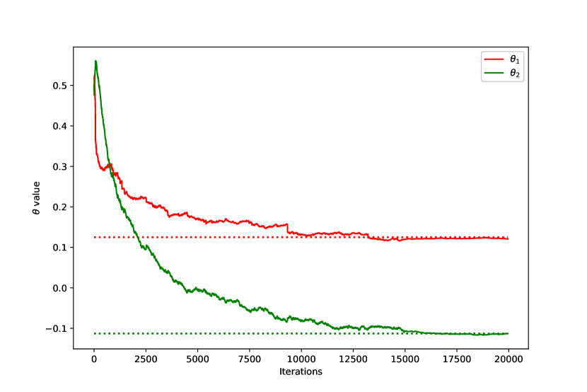
(a) Convergence of parameters $(\theta_{1},\theta_{2})$

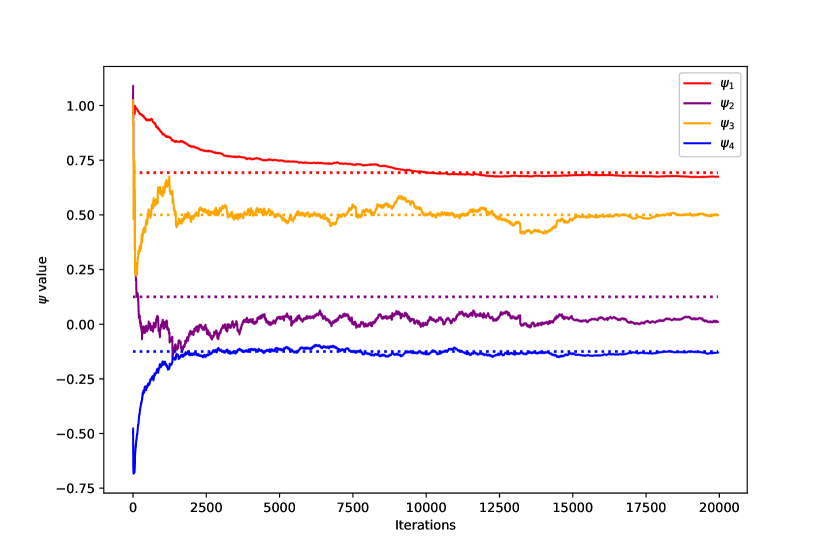
(b) Convergence of parameters $(\psi_{1},\psi_{2},\psi_{3},\psi_{4})$

(c) Value functions under the learnt and true policies

Figure 3:

7.2 Non-LQ MFG and MFC examples on jump control

In this subsection, we consider a jump-diffusion state process given by

$$dX^{\bm{\pi}}_{s}=X^{\bm{\pi}}_{s-}(a_{s}^{\bm{\pi}}dN_{s}+\sigma dW_{s}),$$ (7.7)

where $dN_{s}$ is a Poisson process with intensity $\eta>0$. Let us consider the following objective function for the jump control in the form of

$$J(t,x,\mu;\widehat{\bm{\pi}},\bm{\pi})= \mathbb{E}^{e}\left[\log\left(\frac{X_{T}^{t,x,\mu,\widehat{\bm{\pi}}}}{\mathbb{E}^{e}[X^{t,\xi,\bm{\pi}}_{T}]}\right)-r_{0}\int_{t}^{T}\frac{X_{s}^{t,x,\mu,\widehat{\bm{\pi}}}}{\mathbb{E}^{e}[X^{t,\xi,\bm{\pi}}_{s}]}(1+a_{s}^{\widehat{\bm{\pi}}})ds\right]$$ (7.8)

$$-\gamma\int_{t}^{T}\log\widehat{\bm{\pi}}(a^{\widehat{\bm{\pi}}}_{s}|s,X_{s}^{t,x,\mu,\widehat{\bm{\pi}}},\mu^{\bm{\pi}}_{s})ds\biggl{]}.$$

In other words, we take $\beta=0$, $r(t,x,\mu,a)=-r_{0}(1+a)x/\bar{\mu}$ and $g(x,\mu)=\log x-\log(\bar{\mu})$ in (2.2). We assume that $r_{0}\geq\gamma>0$ in this example.

Remark 7.2.

• (7.7) can be rewritten as

  $$X_{t}=X_{0}\cdot\Big{[}\prod_{k:\tau_{k}\leq t}(1+a_{\tau_{k}})\Big{]}\cdot\exp\Big{(}-\frac{1}{2}\sigma^{2}t+\sigma W_{t}\Big{)},$$

  where $\{\tau_{j}\}_{j=1}^{\infty}$ are jump times of the Poisson process with intensity $\eta$. That is to say, the agent controls the growth rate (or depreciation rate if $a<0$) of $X$ at Poisson arrival times. However, the arrival intensity $\eta$ and the volatility of Gaussian noise $\sigma$ are unknown to the agent, which requires him to learn these parameters and optimize the object (7.8) simultaneously.

• The first term of (7.8) can be understood as the expected utility of the random variable $\frac{X^{t,x,\mu,\widehat{\bm{\pi}}}_{T}}{\mathbb{E}^{e}[X^{t,\xi,\bm{\pi}}_{T}]}$. In other words, the final outcome is not $X_{T}$ itself, but rather, its ratio with respect to some expected values. This ratio (at time $s\in[0,T]$) also determines the instantaneous cost in our setting. In MFG problems, the expected values are from population states, while in MFC problems, it can be understood as a benchmark.

In this subsection we consider problem (7.8) in the context of MFG and MFC, and utilize RL approach to deal with unknown parameters in both formulations.

7.2.1 The MFG problem on jump control

To facilitate exact parameterization of RL algorithm, we first solve the problem explicitly. By calculating (2.11) and (2.10), we derive the explicit expression of the MFE policy and associated game value function. The MFE is of a Gamma type such that

$$\bm{\pi}^{MFG,*}(a|t,x,\mu)={\rm Gamma}\Bigg{(}\big{(}\frac{\eta}{\gamma}+1\big{)}e^{\eta(t-T)},\frac{r_{0}x}{\gamma\bar{\mu}}\Bigg{)}-1,$$ (7.9)

and the decoupled value function takes the form

$$J^{MFG,*}_{d}(t,x,\mu)= \left(\left(1+\frac{\gamma}{\eta}\right)e^{\eta(t-T)}-\frac{\gamma}{\eta}\right)\log\left(\frac{x}{\bar{\mu}}\right)+K_{1}(t-T)+K_{2}(e^{\eta(t-T)}-1)$$ (7.10)

$$+K_{3}(e^{2\eta(t-T)}-1)+\gamma\int_{t}^{T}\log\Gamma\Big{(}\frac{\gamma+\eta}{\gamma}e^{\eta(s-T)}\Big{)}ds,$$

where the distribution ${\rm Gamma}(\alpha,\beta)$ has the density function $f_{\alpha,\beta}(z)=\frac{\beta^{\alpha}}{\Gamma(\alpha)}z^{\alpha-1}e^{-\beta z}$, $z>0$, and constants $K_{i}$, $1\leq i\leq 3$ are given by

$$K_{1}=-\gamma\Big{(}\frac{\sigma^{2}}{2\eta}-1\Big{)},\;K_{2}=-\frac{(\eta+\gamma)(r_{0}+\gamma)}{r_{0}\eta}-\frac{\gamma+\eta}{\eta}\log\Big{(}\frac{\gamma}{r_{0}}\Big{)}+\frac{\sigma^{2}(\gamma+\eta)}{2\eta^{2}},\;K_{3}=\frac{(\eta+\gamma)^{2}}{2\eta r_{0}}.$$

The details of the calculation can be found in Appendix A.9.

Remark 7.3.

For the MFE policy in (A.41), we can derive the variance of the randomized policy as

$$\text{Var}(\bm{\pi}^{MFG,*})=\frac{(\frac{\eta}{\gamma}+1)e^{\eta(t-T)}\gamma^{2}(\bar{\mu})^{2}}{r_{0}^{2}x^{2}}.$$

It is interesting to see that the variance is again decreasing in $\eta$, i.e., the larger jump risk intensity results in the smaller variance of the randomized MFE policy in this particular MFG example. It is also easy to see that if the temperature parameter $\gamma=0$, the variance of the policy is also $0$ and hence the MFE policy degenerates to a constant policy.

From Definition 3.1, we obtain the decoupled Iq-function explicitly as

$$q_{d}^{MFG,*}(t,x,\mu,a,{\bm{h}})= (\gamma+\eta)e^{\eta(t-T)}(\log x-\log\bar{\mu})+[(\gamma+\eta)e^{\eta(t-T)}-\gamma]\log(1+a)-r_{0}\frac{x}{\bar{\mu}}(1+a)$$

$$-\frac{(\gamma+\eta)e^{\eta(t-T)}-\gamma}{\bar{\mu}}\mathbb{E}^{e}_{\mu,{\bm{h}}}[\xi a^{{\bm{h}}}]-(\gamma+\eta)e^{\eta(t-T)}\log(\gamma/r_{0})-\gamma\log\Gamma\Bigg{(}\frac{(\gamma+\eta)e^{\eta(t-T)}}{\gamma}\Bigg{)}$$

$$+\big{(}(\gamma+\eta)e^{\eta(t-T)}-\gamma\big{)}\cdot\Big{(}\frac{(\gamma+\eta)e^{\eta(t-T)}}{r_{0}}-1\Big{)}.$$ (7.11)

Thanks to the explicit expressions of the decoupled value function in (7.10) and associated decoupled Iq-function in (7.11), we can consider the parametrized approximators $J_{d}^{\theta}$ and $q_{d}^{\psi}$ in Algorithm 1 as follows:

$$J_{d}^{\theta}(t,x,\mu)= [(1+\theta_{1})e^{\theta_{2}(t-T)}-\theta_{1}](\log x-\log\bar{\mu})+\theta_{3}(t-T)+\theta_{4}(e^{\theta_{2}(t-T)}-1)$$ (7.12)

$$+\theta_{5}(e^{2\theta_{2}(t-T)}-1)+\gamma\int_{t}^{T}\log\Gamma(e^{\theta_{2}(s-T)+\theta_{6}})ds.$$

$${q}_{d}^{\psi}(t,x,\mu,a,{\bm{h}})= e^{\psi_{1}+\psi_{2}(t-T)}(\log x-\log\bar{\mu})+[e^{\psi_{1}+\psi_{2}(t-T)}-\gamma]\log(1+a)-(\gamma+e^{\psi_{3}})\frac{x}{\bar{\mu}}(1+a)$$

$$-\frac{e^{\psi_{1}+\psi_{2}(t-T)}-\gamma}{\bar{\mu}}\mathbb{E}^{e}_{\mu,{\bm{h}}}[\xi a^{{\bm{h}}}]-e^{\psi_{1}+\psi_{2}(t-T)}\log\Big{(}\frac{\gamma}{\gamma+e^{\psi_{3}}}\Big{)}-\gamma\log\Gamma\Big{(}\frac{e^{\psi_{1}+\psi_{2}(t-T)}}{\gamma}\Big{)}$$

$$+\big{(}e^{\psi_{1}+\psi_{2}(t-T)}-\gamma\big{)}\cdot\Big{(}\frac{e^{\psi_{1}+\psi_{2}(t-T)}}{\gamma+e^{\psi_{3}}}-1\Big{)}.$$ (7.13)

We also know the true values of the above parameters as

$$\theta_{1}^{*}=\gamma/\eta,\quad\theta^{*}_{2}=\eta,\quad\theta_{3}^{*}=-\gamma\Big{(}\frac{\sigma^{2}}{2\eta}-1\Big{)},$$

$$\theta_{4}^{*}=-\frac{(\gamma+\eta)(r_{0}+\gamma)}{r_{0}\eta}-\frac{\gamma+\eta}{\eta}\log\Big{(}\frac{\gamma}{r_{0}}\Big{)}+\frac{\sigma^{2}(\gamma+\eta)}{2\eta^{2}},$$

$$\theta_{5}^{*}=\frac{(\eta+\gamma)^{2}}{2\eta r_{0}},\quad\theta_{6}^{*}=\log\Big{(}\frac{\gamma+\eta}{\gamma}\Big{)}.$$

$$\psi_{1}^{*}=\log(\gamma+\eta),\quad\psi_{2}^{*}=\eta,\quad\psi_{3}^{*}=\log(r_{0}-\gamma).$$

Consequently, with the learnt parameters $(\theta,\psi)$, the approximated MFE policy is derived from (5.2) as

$$\bm{\pi}^{\psi}(a|t,x,\mu)={\rm Gamma}\Big{(}\frac{e^{\psi_{1}+\psi_{2}(t-T)}}{\gamma},\frac{(e^{\psi_{3}}+\gamma)x}{\gamma\bar{\mu}}\Big{)}-1,$$ (7.14)

and in each iteration of Algorithm 1 we use the test policy with same form but with different parameters $\tilde{\psi}$:

$${\bm{h}}^{\tilde{\psi}}(a|t,x,\mu)={\rm Gamma}\Big{(}\frac{e^{\tilde{\psi}_{1}+\tilde{\psi}_{2}(t-T)}}{\gamma},\frac{(e^{\tilde{\psi}_{3}}+\gamma)x}{\gamma\bar{\mu}}\Big{)}-1.$$

Finally, it is easy to check that $q_{d}^{\psi}$ in (7.13) and ${\bm{\pi}}^{\psi}$ in (7.14) satisfy the consistency condition (4.3)-(4.4).

Let us discuss the environment simulator that will be used in the learning context of both MFG and MFC.
The Simulator Environment_Δt. In the learning phase, for each time step $t_{k}$, the representative agent takes the action $a_{t_{k}}\sim{\bm{h}}^{\tilde{\psi}}(\cdot|t_{k},X_{t_{k}},\bar{\mu}_{estimate,t_{k}})$, and the state at $t_{k+1}$ is given by

$$X_{t_{k+1}}=X_{t_{k}}\cdot(1+a_{t_{k}})^{\triangle N_{\eta,\Delta t}}\cdot\exp\big{\{}\sigma\sqrt{\Delta t}\triangle W-\frac{1}{2}\sigma^{2}\Delta t\big{\}},$$ (7.15)

where $\triangle W\sim{\cal N}(0,1)$, and $\triangle N_{\eta,\Delta t}\sim{\rm Poisson}(\eta\Delta t)$. In the meantime, the reward is generated by

$$r_{t_{k}}=-r_{0}(1+a_{t_{k}})X_{t_{k}}/\bar{\mu}_{t_{k},true}.$$ (7.16)

We then apply Algorithm 1 to the MFG jump control problem, with parameterizations given in (7.12)-(7.13). We set $T=1$, $\gamma=0.5$, $\eta=1.5$, $r_{0}=1$ and $\sigma=0.5$ for the simulator. We also choose $K=20$, $M=20$ and $N=7000$. The lower and upper bounds of uniform distribution for test policies are $p_{1}=p_{2}=p_{3}=0$ and $q_{1}(j)=q_{2}(j)=q_{3}(j)=\frac{1}{j^{0.5}}$. Meanwhile, we set learning rates as

$$\alpha_{\theta}(j)=\left\{\begin{aligned} &\left(\frac{0.005}{j^{0.31}},\frac{0.013}{j^{0.31}},\frac{0.019}{j^{0.31}},\frac{0.013}{j^{0.31}},\frac{0.008}{j^{0.31}},\frac{0.015}{j^{0.31}}\right),&0\leq j<3500,\\ &\left(\frac{0.005}{j^{0.61}},\frac{0.013}{j^{0.61}},\frac{0.019}{j^{0.61}},\frac{0.013}{j^{0.61}},\frac{0.008}{j^{0.61}},\frac{0.015}{j^{0.61}}\right),&j\geq 3500,\end{aligned}\right.$$

$$\alpha_{\psi}(j)=\left\{\begin{aligned} &\left(\frac{0.013}{j^{0.31}},\frac{0.013}{j^{0.61}},\frac{0.015}{j^{0.31}}\right),&0\leq j<3500,\\ &\left(\frac{0.013}{j^{0.31}},\frac{0.013}{j^{0.61}},\frac{0.015}{j^{0.31}}\right),&j\geq 3500.\end{aligned}\right.$$

The parameters are initialized as $\theta=(0,2,2,1,2,1)$ and $\psi=(-1,2,2)$. We display the convergence of parameter iterations in Figures 4(a), 4(b) and 4(c). The comparison between learnt and true parameters is reported in Table 2. Similar as the mean-variance control problem, we also compare the values under the learnt policy and the true policy with two populations of 10000 agents in Figure 4(d).

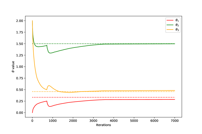
(a) Convergence of parameters $(\theta_{1},\ldots,\theta_{3})$

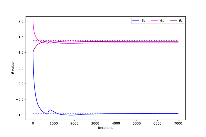
(b) Convergence of parameters $(\theta_{4},\ldots,\theta_{6})$

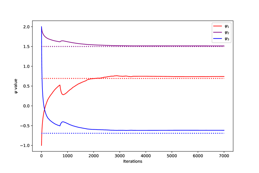
(c) Convergence of parameters $(\psi_{1},\ldots,\psi_{3})$

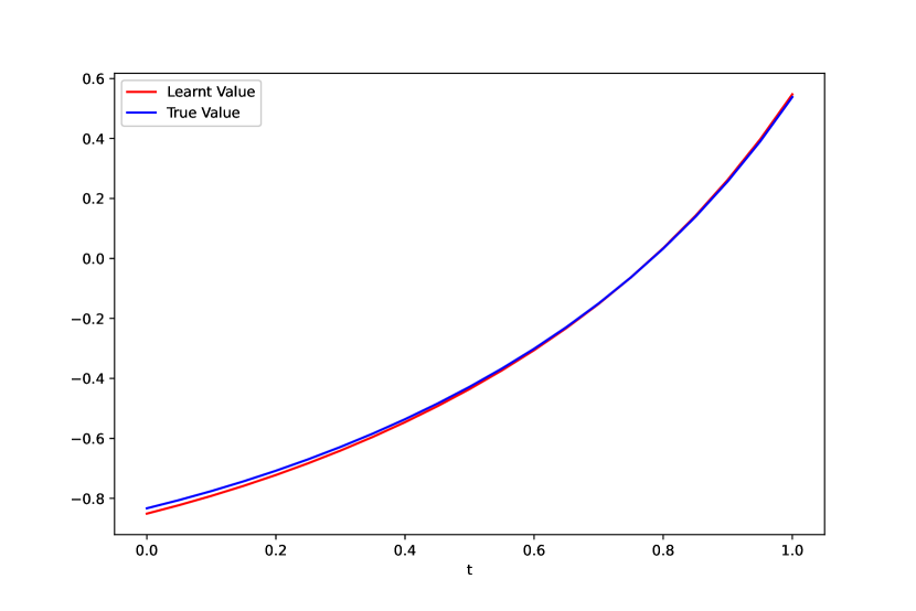
(d) Value functions under the learnt and true policies

Figure 4:

	$\theta_{1}$	$\theta_{2}$	$\theta_{3}$	$\theta_{4}$	$\theta_{5}$	$\theta_{6}$	$\psi_{1}$	$\psi_{2}$	$\psi_{3}$
True Value	0.333	1.5	0.458	-0.965	1.333	1.386	0.693	1.5	-0.693
Learnt Value	0.287	1.497	0.482	-0.951	1.307	1.343	0.741	1.515	-0.618

Table 2: Learnt v.s. true parameters

7.2.2 The MFC problem on jump control

Similar to the previous MFG problem, we can also derive the explicit solution of the mean-filed optimal policy and the associated decoupled value function by solving (2.12) and (2.8). The mean-field optimal policy is also of a Gamma type that

$$\bm{\pi}^{MFC,*}(a|t,x,\mu)={\rm Gamma}\Big{(}\big{(}\frac{\eta}{\gamma}+1\big{)}e^{\eta(t-T)},\big{(}r_{0}-\gamma+(\eta+\gamma)e^{\eta(t-T)}\big{)}\frac{x}{\gamma\bar{\mu}}\Big{)}-1.$$ (7.17)

The associated decoupled value function is of the form

$$J^{MFC,*}_{d}(t,x,\mu)= \left(\left(1+\frac{\gamma}{\eta}\right)e^{\eta(t-T)}-\frac{\gamma}{\eta}\right)\log(x/\bar{\mu})+K_{1}^{\prime}(t-T)+K_{2}^{\prime}(e^{\eta(t-T)}-1)$$ (7.18)

$$+K_{3}^{\prime}\big{(}\log\big{(}(\gamma+\eta)e^{\eta(t-T)}+r_{0}-\gamma\big{)}-\log(\eta+r_{0})\big{)}+\gamma\int_{t}^{T}\log\Gamma\big{(}\frac{\gamma+\eta}{\gamma}e^{\eta(s-T)}\big{)}ds$$

$$+{K_{4}^{\prime}\big{(}e^{\eta(t-T)}\log\big{(}(\gamma+\eta)e^{\eta(t-T)}+r_{0}-\gamma\big{)}-\log(r_{0}+\eta)\big{)}},$$

where constants $K^{\prime}_{i}$, $1\leq i\leq 4$ are given by

$$K_{1}^{\prime}=-\gamma\Big{(}\frac{\sigma^{2}}{2\eta}-1\Big{)},\quad K_{2}^{\prime}=\frac{\gamma+\eta}{\eta}\Big{[}\frac{\sigma^{2}}{2\eta}-2-\log\gamma\Big{]},\quad K^{\prime}_{3}=\frac{r_{0}-\gamma}{\eta},\quad K_{4}^{\prime}=\frac{\gamma+\eta}{\eta}.$$

We obtain from Definition 3.1 the explicit expression of the decoupled Iq-function

$$q_{d}^{*}(t,x,\mu,a,{\bm{h}})= (\eta+\gamma)e^{\eta(t-T)}(\log x-\log\bar{\mu})+[(\gamma+\eta)e^{\eta(t-T)}-\gamma]\log(1+a)-r_{0}\frac{x}{\bar{\mu}}(1+a)$$

$$-\frac{(\gamma+\eta)e^{\eta(t-T)}-\gamma}{\bar{\mu}}\mathbb{E}^{e}_{\mu,{\bm{h}}}[\xi a^{\bm{h}}]-(\eta+\gamma)(1+\log\gamma)e^{\eta(t-T)}+\gamma$$ (7.19)

$$-\gamma\log\Gamma\Big{(}\frac{(\gamma+\eta)e^{\eta(t-T)}}{\gamma}\Big{)}+(\gamma+\eta)e^{\eta(t-T)}\log\big{(}(\gamma+\eta)e^{\eta(t-T)}+r_{0}-\gamma\big{)}.$$

The calculation is deferred to Appendix A.10.

Remark 7.4.

For this MFC example and its optimal policy ${\bm{\pi}}^{MFC,*}$ in (7.17), we can derive that

$$\text{Var}({\bm{\pi}}^{MFC,*})=\frac{(\frac{\eta}{\gamma}+1)e^{\eta(t-T)}\gamma^{2}(\bar{\mu})^{2}}{(r_{0}-\gamma+(\eta+\gamma)e^{\eta(t-T)})^{2}x^{2}}.$$

It is easy to check that the variance is no longer monotone in the risk jump intensity $\eta$ as the previous examples. Only when $\eta$ is large enough, the variance of the randomized policy is decreasing in term of $\eta$. Moreover, it is trivial to see that when the temperature parameter $\gamma$ tends 0, the randomized policy will degenerate to the constant policy.

Similar to the MFG problem, we can consider the exact parametrizations of $J_{d}^{\theta}$ and $q_{d}^{\psi}$ as follows based on the above explicit expressions that

$$J_{d}^{\theta}(t,x,\mu)= [(1+\theta_{1})e^{\theta_{2}(t-T)}-\theta_{1}](\log x-\log\bar{\mu})+\theta_{3}(t-T)+\theta_{4}(e^{\theta_{2}(t-T)}-1)$$ (7.20)

$$+e^{\theta_{5}}\big{(}\log\big{(}e^{\theta_{6}+\theta_{2}(t-T)}+e^{\theta_{5}}\big{)}-\log(e^{\theta_{6}}+e^{\theta_{5}})\big{)}+\gamma\int_{t}^{T}\log\Gamma(e^{\theta_{2}(s-T)+\theta_{7}})ds$$

$$+e^{\theta_{6}}\big{(}e^{\theta_{2}(t-T)}\log\big{(}\theta_{2}(e^{\theta_{6}+\theta_{2}(t-T)}+e^{\theta_{5}})\big{)}-\log\big{(}\theta_{2}(e^{\theta_{6}}+e^{\theta_{5}})\big{)}\big{)}.$$

$$q_{d}^{\psi}(t,x,\mu,a,{\bm{h}})= e^{\psi_{1}+\psi_{2}(t-T)}(\log x-\log\bar{\mu})+[e^{\psi_{1}+\psi_{2}(t-T)}-\gamma]\log(1+a)-(\gamma+e^{\psi_{3}})\frac{x}{\bar{\mu}}(1+a)$$

$$-\frac{e^{\psi_{1}+\psi_{2}(t-T)}-\gamma}{\bar{\mu}}\mathbb{E}^{e}_{\mu,{\bm{h}}}[\xi a^{{\bm{h}}}]-(1+\log\gamma)e^{\psi_{1}+\psi_{2}(t-T)}+\gamma-\gamma\log\Gamma\Big{(}\frac{e^{\psi_{1}+\psi_{2}(t-T)}}{\gamma}\Big{)}$$

$$+e^{\psi_{1}+\psi_{2}(t-T)}\log\big{(}e^{\psi_{1}+\psi_{2}(t-T)}+e^{\psi_{3}}\big{)}.$$ (7.21)

The parameterized optimal policy is derived from (7.17) as

$${\bm{\pi}}^{\psi}(a|t,x,\mu)=\Gamma\Big{(}\frac{e^{\psi_{1}+\psi_{2}(t-T)}}{\gamma},\frac{e^{\psi_{1}+\psi_{2}(t-T)+e^{\psi_{3}}}}{\gamma}\frac{x}{\bar{\mu}}\Big{)}-1.$$ (7.22)

Furthermore, it is straightforward to verify that $q_{d}^{\psi}$ and ${\bm{\pi}}^{\psi}$ satisfy the consistency condition (4.5)-(4.6). Note that the true values of parameters are given by

$$\theta_{1}^{*}=\frac{\gamma}{\eta},\;\theta_{2}^{*}=\eta,\;\theta_{3}^{*}=-\gamma(\frac{\sigma^{2}}{2\eta}-1),\;\theta_{4}^{*}=\frac{\gamma+\eta}{\eta}\Big{[}\frac{\sigma^{2}}{2\eta}-2-\log\gamma\Big{]},\quad\theta_{5}^{*}=\log(\frac{r_{0}-\gamma}{\eta}),$$

$$\theta_{6}^{*}=\log(\frac{\gamma+\eta}{\eta}),\quad\theta_{7}^{*}=\log(\frac{\gamma+\eta}{\gamma}),\quad\psi_{1}^{*}=\log(\gamma+\eta),\;\psi_{2}^{*}=\eta,\;\psi_{3}^{*}=\log(r_{0}-\gamma).$$

As in the previous MFG jump control problem, we apply Algorithm 1 to the MFC jump control problem, with parameterizations given in (7.20)-(7.21). To better compare our numerical experiments between MFG and MFC problems, all parameters for MFC are set the same as that for MFG. The learning rates are chosen as

$$\alpha_{\theta}(j) =\left(\frac{0.009}{j^{0.31}},\frac{0.009}{j^{0.11}},0.03,\frac{0.06}{j^{0.12}},\frac{0.05}{j^{0.31}},0.005,0.016\right),$$

$$\alpha_{\psi}(j) =\left(0.008,0.005,0.01\right).$$

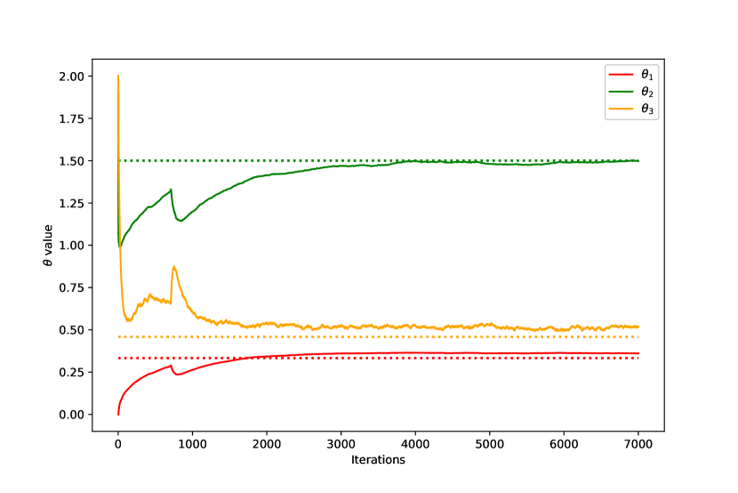
(a) Convergence of parameters $(\theta_{1},\ldots,\theta_{3})$

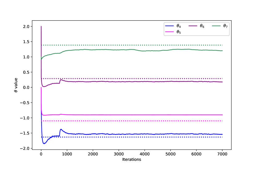
(b) Convergence of parameters $(\theta_{4},\ldots,\theta_{7})$

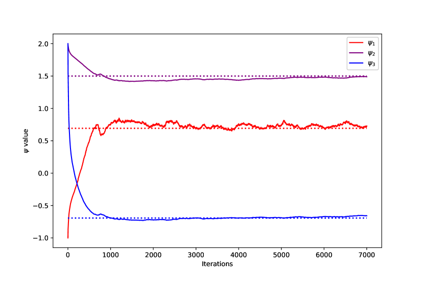
(c) Convergence of parameters $(\psi_{1},\ldots,\psi_{3})$

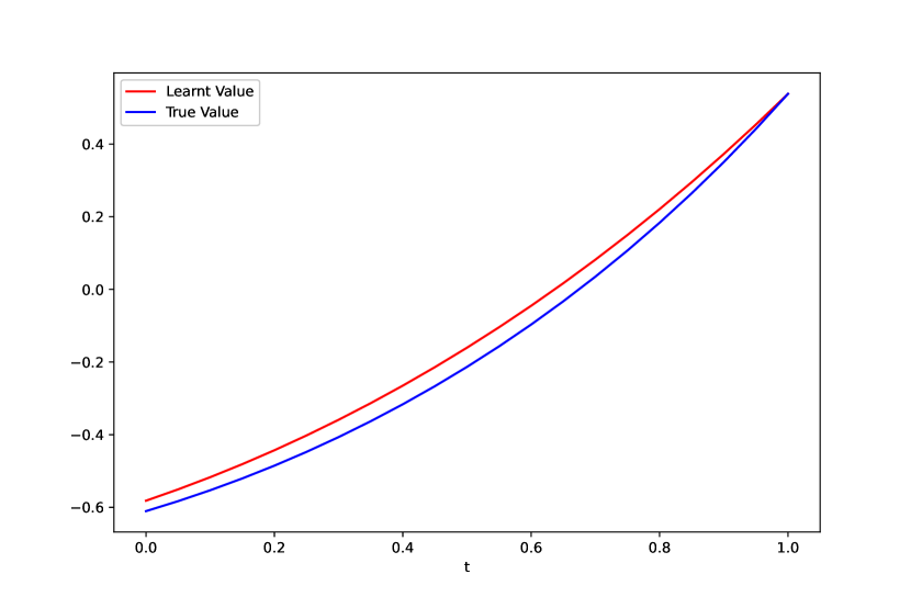
(d) Value functions under the learnt and true policies

Figure 5:

	$\theta_{1}$	$\theta_{2}$	$\theta_{3}$	$\theta_{4}$	$\theta_{5}$	$\theta_{6}$	$\theta_{7}$	$\psi_{1}$	$\psi_{2}$	$\psi_{3}$
True Value	0.333	1.5	0.458	-1.631	-1.099	0.288	1.386	0.693	1.5	-0.693
Learnt Value	0.361	1.49	0.518	-1.542	-0.901	0.177	1.203	0.729	1.489	-0.657

Table 3: Learnt v.s. true parameters

Meanwhile, the parameters are initialized as $\theta=(0,2,2,0,0,2,1)$ and $\psi=(-1,2,2)$. The convergence results of the parameter iterations are illustrated in Figures 5(a), 5(b) and 5(c). A summary of the learned and true parameters is provided in Table 3. We also compare the value functions under the learned policy and the true policy in Figure 5(d). As a by-product, we observe that the cumulative pay-offs at the initial time $0$ under the learned optimal policy in the MFC problem is bigger than those from the learned MFE policy in the MFG problem. Their discrepancy can be interpreted as the Price of Anarchy (PoA) firstly introduced in Koutsoupias and Papadimitriou (1999).

Acknowledgement: X. Wei is supported by National Natural Science Foundation of China grant under no.12201343. X. Yu is supported by the Hong Kong RGC General Research Fund (GRF) under grant no. 15211524.

Appendix A Proofs

This appendix reports the proofs of all main results in previous sections.

A.1 Proof of Proposition 2.6

Proof.

For any test function $v\in C_{b}^{2}(\mathbb{R}^{d})$, we have

$$\int_{{\cal A}}{\cal L}^{t,a,\mu}[v(\cdot)](x){\bm{\pi}}(a|t,x,\mu)da$$

$$= b_{\bm{\pi}}(t,x,\mu)^{\scriptscriptstyle{\intercal}}\partial_{x}v(x)+\frac{1}{2}{\rm Tr}\big{(}\sigma_{\bm{\pi}}\sigma_{\bm{\pi}}^{\scriptscriptstyle{\intercal}}(t,x,\mu)\partial_{xx}v(x)\big{)}$$

$$+\int_{{\cal A}}\big{[}v(x+\Gamma(t,x,a,\mu))-v(x)-\Gamma(t,x,a,\mu)^{\scriptscriptstyle{\intercal}}\partial_{x}v(x)\big{]}\eta(t){\bm{\pi}}(a|t,x,\mu)da$$

$$= b_{\bm{\pi}}(t,x,\mu)^{\scriptscriptstyle{\intercal}}\partial_{x}v(x)+\frac{1}{2}{\rm Tr}\big{(}\sigma_{\bm{\pi}}\sigma_{\bm{\pi}}^{\scriptscriptstyle{\intercal}}(t,x,\mu)\partial_{xx}v(x)\big{)}$$

$$+\int_{\mathbb{R}^{d}}\big{[}v(x+y)-v(x)-y^{\scriptscriptstyle{\intercal}}\partial_{x}v(x)\big{]}\eta(t)\Gamma(t,x,\mu,\cdot)_{\#}{\bm{\pi}}(\cdot,t,x,\mu)(dy)$$

$$= b_{\bm{\pi}}(t,x,\mu)^{\scriptscriptstyle{\intercal}}\partial_{x}v(x)+\frac{1}{2}{\rm Tr}\big{(}\sigma_{\bm{\pi}}\sigma_{\bm{\pi}}^{\scriptscriptstyle{\intercal}}(t,x,\mu)\partial_{xx}v(x)\big{)}$$

$$+\int_{\mathbb{R}^{d}}\big{[}v(x+y)-v(x)-y^{\scriptscriptstyle{\intercal}}\partial_{x}v(x)\big{]}\eta(t)\Gamma_{\bm{\pi}}(t,x,\mu,\cdot)_{\#}\mu_{0}(dy)$$

$$= b_{\bm{\pi}}(t,x,\mu)^{\scriptscriptstyle{\intercal}}\partial_{x}v(x)+\frac{1}{2}{\rm Tr}\big{(}\sigma_{\bm{\pi}}\sigma_{\bm{\pi}}^{\scriptscriptstyle{\intercal}}(t,x,\mu)\partial_{xx}v(x)\big{)}$$

$$+\int_{\mathbb{R}}\big{[}v(x+\Gamma_{\bm{\pi}}(t,x,\mu,z))-v(x)-\Gamma_{\bm{\pi}}(t,x,\mu,z)^{\scriptscriptstyle{\intercal}}\partial_{x}v(x)\big{]}\eta(t)\mu_{0}(dz).$$

As a result, we have constructed another pair of processes $(\hat{X}^{t,x,\mu,\widehat{\bm{\pi}}},\hat{X}^{t,\xi,\widehat{\bm{\pi}}})$ equal to $({X}^{t,x,\mu,\widehat{\bm{\pi}}},{X}^{t,\xi,{\bm{\pi}}})$ in law, satisfying similar SDEs as (2.3)-(2.4), with $\Gamma$ replaced by $\Gamma_{\bm{\pi}}$ and the jump measure replaced by the one with the compensator $\mu_{0}(dz)\eta(t)dt$. Thus, we can combine the results in Frikha et al. (2023), Hao and Li (2016) and Li (2018) to complete the proof. ∎

A.2 Proof of Theorem 4.1

Proof.

We first show that if $\widehat{J}_{d}(\cdot)=J_{d}(\cdot;\widehat{\bm{\pi}},{\bm{\pi}})$ and $\widehat{q}_{d}(\cdot)=q_{d}(\cdot;\widehat{\bm{\pi}},{\bm{\pi}})$, then (4.1)-(4.2) holds. It is straightforward to see from (2.8) and (3.3) that the (4.1) holds.

By applying Itô’s formula to $\widehat{J}_{d}(t^{\prime},X_{t^{\prime}}^{R,{\bm{h}}},\mu_{t^{\prime}}^{{\bm{h}}})$ between $t$ and $s$, $0\leq t<s\leq T$, we get that

$$e^{-\beta s}\widehat{J}_{d}(s,X_{s}^{R,{\bm{h}}},\mu_{s}^{{\bm{h}}})-e^{-\beta t}\widehat{J}_{d}(t,x,\mu)+\int_{t}^{s}e^{-\beta t^{\prime}}\Big{[}r(t^{\prime},X_{t^{\prime}}^{R,{\bm{h}}},\mu_{t^{\prime}}^{{\bm{h}}},{a}_{t^{\prime}}^{{\bm{h}}})-\widehat{q}_{d}(t^{\prime},X_{t^{\prime}}^{R,{\bm{h}}},\mu_{t^{\prime}}^{{\bm{h}}},{a}^{{\bm{h}}}_{t^{\prime}},{\bm{h}})\Big{]}dt^{\prime}$$

$$= \int_{t}^{s}e^{-\beta t^{\prime}}\biggl{(}\frac{\partial}{\partial t}\widehat{J}_{d}(t^{\prime},X_{t^{\prime}}^{R,{\bm{h}}},\mu_{t^{\prime}}^{{\bm{h}}})-\beta\widehat{J}_{d}(t^{\prime},X_{t^{\prime}}^{R,{\bm{h}}},\mu_{t^{\prime}}^{{\bm{h}}})+\mathcal{L}^{t^{\prime},a^{{\bm{h}}},\mu_{t^{\prime}}^{\bm{h}}}[\widehat{J}_{d}(t^{\prime},\cdot,\mu_{t^{\prime}}^{\bm{h}})](X_{t^{\prime}}^{R,{\bm{h}}})+r(t^{\prime},X_{t^{\prime}}^{R,{\bm{h}}},\mu_{t^{\prime}}^{\bm{h}},a^{{{\bm{h}}}}_{t^{\prime}})$$

$$+\int_{\mathbb{R}^{d}\times{\cal A}}{\cal L}^{t^{\prime},a,\mu_{t^{\prime}}^{\bm{h}}}[\frac{\delta\widehat{J}_{d}}{\delta\mu}(t,X_{t^{\prime}}^{R,{\bm{h}}},\mu_{t^{\prime}}^{\bm{h}})(\cdot)](y){\bm{h}}(a|t^{\prime},y,\mu_{t^{\prime}}^{\bm{h}})da\mu_{t^{\prime}}^{\bm{h}}(da)-\widehat{q}_{d}(t^{\prime},X_{t^{\prime}}^{R,{\bm{h}}},\mu_{t^{\prime}}^{{\bm{h}}},a^{{{\bm{h}}}}_{t^{\prime}},{\bm{h}})\biggl{)}dt^{\prime}$$

$$+\int_{t}^{s}e^{-\beta t^{\prime}}\partial_{x}\widehat{J}_{d}(t^{\prime},X_{t^{\prime}}^{R,{\bm{h}}},\mu_{t^{\prime}}^{{\bm{h}}})^{\scriptscriptstyle{\intercal}}\sigma(t^{\prime},X_{t^{\prime}}^{R,{\bm{h}}},\mu_{t^{\prime}}^{{\bm{h}}},a^{{\bm{h}}}_{t^{\prime}})dW_{t^{\prime}}$$

$$+\int_{t}^{s}e^{-\beta t^{\prime}}\Big{\{}\widehat{J}_{d}(t^{\prime},X_{t^{\prime}-}^{R,{\bm{h}}}+\Gamma(t^{\prime},X_{t^{\prime}}^{R,{\bm{h}}},\mu_{t^{\prime}}^{{\bm{h}}},a^{{\bm{h}}}_{t^{\prime}}),\mu_{t^{\prime}}^{{\bm{h}}})-\widehat{J}_{d}(s,X_{t^{\prime}-}^{R,{\bm{h}}},\mu_{t^{\prime}}^{{\bm{h}}})\Big{\}}d\widetilde{N}_{t^{\prime}}.$$

$$=: \int_{t}^{s}e^{-\beta t^{\prime}}\biggl{(}\check{q}_{d}(t^{\prime},X_{t^{\prime}}^{R,{\bm{h}}},\mu_{t^{\prime}}^{{\bm{h}}},a^{{{\bm{h}}}}_{t^{\prime}},{\bm{h}})-\widehat{q}_{d}(t^{\prime},X_{t^{\prime}}^{R,{\bm{h}}},\mu_{t^{\prime}}^{{\bm{h}}},a^{{{\bm{h}}}}_{t^{\prime}},{\bm{h}})\biggl{)}dt^{\prime}$$

$$+\int_{t}^{s}e^{-\beta t^{\prime}}\partial_{x}\widehat{J}_{d}(t^{\prime},X_{t^{\prime}}^{R,{\bm{h}}},\mu_{t^{\prime}}^{{\bm{h}}})^{\scriptscriptstyle{\intercal}}\sigma(t^{\prime},X_{t^{\prime}}^{R,{\bm{h}}},\mu_{t^{\prime}}^{{\bm{h}}},a^{{\bm{h}}}_{t^{\prime}})dW_{t^{\prime}}$$ (A.1)

$$+\int_{t}^{s}e^{-\beta t^{\prime}}\Big{\{}\widehat{J}_{d}(t^{\prime},X_{t^{\prime}-}^{R,{\bm{h}}}+\Gamma(t^{\prime},X_{t^{\prime}}^{R,{\bm{h}}},\mu_{t^{\prime}}^{{\bm{h}}},a^{{\bm{h}}}),\mu_{t^{\prime}}^{{\bm{h}}})-\widehat{J}_{d}(s,X_{t^{\prime}-}^{R,{\bm{h}}},\mu_{t^{\prime}}^{{\bm{h}}})\Big{\}}d\widetilde{N}_{t^{\prime}},$$

where $\check{q}_{d}$ is defined by

$$\check{q}_{d}(t,x,\mu,a,{\bm{h}}) :=\frac{\partial\widehat{J}_{d}}{\partial t}(t,x,\mu)-\beta\widehat{J}_{d}(t,x,\mu)+\mathcal{L}^{t,a,\mu}[\widehat{J}_{d}(t,\cdot,\mu)](x)+r(t,x,\mu,a)$$ (A.2)

$$+\mathbb{E}_{\mu,{\bm{h}}}\Big{[}\mathcal{L}^{t,a^{\bm{h}},\mu}[\frac{\delta\widehat{J}_{d}}{\delta\mu}(t,x,\mu)(\cdot)](\xi)\Big{]}.$$

Taking $\widehat{J}_{d}(\cdot)=J_{d}(\cdot;\widehat{\bm{\pi}},{\bm{\pi}})$ and $\widehat{q}_{d}(\cdot)=q_{d}(\cdot;\widehat{\bm{\pi}},{\bm{\pi}})$ into the above equality (A.1), we obtain

$$e^{-\beta s}\widehat{J}_{d}(s,X_{s}^{R,{\bm{h}}},\mu_{s}^{{\bm{h}}})-e^{-\beta t}\widehat{J}_{d}(t,x,\mu)+\int_{t}^{s}e^{-\beta t^{\prime}}\Big{[}r(t^{\prime},X_{t^{\prime}}^{R,\widehat{\bm{h}}},\mu_{t^{\prime}}^{{\bm{h}}},{a}_{t^{\prime}}^{{\bm{h}}})-\widehat{q}_{d}(t^{\prime},X_{t^{\prime}}^{R,{\bm{h}}},\mu_{t^{\prime}}^{{\bm{h}}},{a}^{{\bm{h}}}_{t^{\prime}},{\bm{h}})\Big{]}dt^{\prime}$$

$$= \int_{t}^{s}e^{-\beta t^{\prime}}\partial_{x}\widehat{J}_{d}(t^{\prime},X_{t^{\prime}}^{R,{\bm{h}}},\mu_{t^{\prime}}^{{\bm{h}}})^{\scriptscriptstyle{\intercal}}\sigma(t^{\prime},X_{t^{\prime}}^{R,{\bm{h}}},\mu_{t^{\prime}}^{{\bm{h}}},a^{{\bm{h}}})dW_{t^{\prime}}$$

$$+\int_{t}^{s}e^{-\beta t^{\prime}}\Big{\{}\widehat{J}_{d}(t^{\prime},X_{t^{\prime}-}^{R,{\bm{h}}}+\Gamma(t^{\prime},X_{t^{\prime}-}^{R,{\bm{h}}},\mu_{t^{\prime}}^{{\bm{h}}},a^{{\bm{h}}})_{t^{\prime}-},\mu_{s}^{{\bm{h}}})-\widehat{J}_{d}(s,X_{t^{\prime}-}^{R,{\bm{h}}},\mu_{t^{\prime}}^{{\bm{h}}})\Big{\}}d\widetilde{N}_{t^{\prime}},$$

which is a $\mathbb{F}^{e}$-adapted martingale under Assumptions 2.4 and 2.5.

Conversely, we prove that if (4.1)-(4.2) holds, then $\widehat{J}_{d}(\cdot)=J(\cdot;\widehat{\bm{\pi}},{\bm{\pi}})$ and $\widehat{q}_{d}(\cdot)=q_{d}(\cdot;\widehat{\bm{\pi}},{\bm{\pi}})$.

In view of (A.1), the equation (4.2) implies that

$$\int_{t}^{s}e^{-\beta t^{\prime}}\biggl{(}\check{q}_{d}(t^{\prime},X_{t^{\prime}}^{R,{\bm{h}}},\mu_{t^{\prime}}^{{\bm{h}}},a^{{\bm{h}}},{\bm{h}})-\widehat{q}_{d}(t^{\prime},X_{t^{\prime}}^{R,{\bm{h}}},\mu_{t^{\prime}}^{{\bm{h}}},a^{{\bm{h}}},{\bm{h}})\biggl{)}dt^{\prime}$$ (A.3)

is a local martingale with finite variation and hence zero quadratic variation. Therefore, $\mathbb{P}^{e}$-almost surely,

$$\int_{t}^{s}e^{-\beta t^{\prime}}\biggl{(}\check{q}_{d}(t^{\prime},X_{t^{\prime}}^{R,{\bm{h}}},\mu_{t^{\prime}}^{{\bm{h}}},a^{{\bm{h}}},{\bm{h}})-\widehat{q}_{d}(t^{\prime},X_{t^{\prime}}^{R,{\bm{h}}},\mu_{t^{\prime}}^{{\bm{h}}},a^{{\bm{h}}},{\bm{h}})\biggl{)}dt^{\prime}=:\int_{t}^{s}e^{-\beta t^{\prime}}f(t^{\prime},X_{t^{\prime}}^{R,{\bm{h}}},\mu_{t^{\prime}}^{{\bm{h}}},a^{{\bm{h}}},{\bm{h}})dt^{\prime}$$

is zero for all $s\in[t,T]$. That is, there exists $\Omega^{c}\in{\cal F}$ with $\mathbb{P}^{e}(\Omega^{c})=1$ such that for any $\omega\in\Omega^{c}$

$$\int_{t}^{s}e^{-\beta t^{\prime}}f(t^{\prime},X_{t^{\prime}}^{R,{\bm{h}}},\mu_{t^{\prime}}^{{\bm{h}}},a^{{\bm{h}}}_{t^{\prime}},{\bm{h}})dt^{\prime}=0,$$ (A.4)

The rest is to show $f(t,x,\mu,a,{\bm{h}})\equiv 0$, which will be verified by the argument of contradiction. Suppose that the claim does not hold. By the continuity of $f$, there exists $(t^{*},x^{*},\mu^{*},a^{*},{\bm{h}}^{*})\in[0,T]\times\mathbb{R}^{d}\times{\cal P}_{2}(\mathbb{R}^{d})\times{\cal A}\times\Pi$ and $\epsilon>0$ such that $f(t^{*},x^{*},\mu^{*},a^{*},{\bm{h}}^{*})>\epsilon$. As $f$ is continuous, there exists $\delta>0$ such that if $\max\{|t-t^{*}|,|x-x^{*}|,{\cal W}_{2}(\mu,\mu^{*}),|a-a^{*}|\}<\delta$, then $f(t,x,\mu,a,{\bm{h}}^{*})>\frac{\epsilon}{2}$. Now let us consider the process $(X^{R,{\bm{h}}^{*}},X^{P,{\bm{h}}^{*}})$ with $X^{R,{\bm{h}}^{*}}_{t^{*}-}=x^{*},X^{P,{\bm{h}}^{*}}_{t^{*}}\sim\mu^{*}$.

Let us define

$$\tau:=\inf\big{\{}s>t^{*}:|X^{R,{\bm{h}}^{*}}_{s-}-x^{*}|>\delta\;\mbox{or}\;{\cal W}_{2}(\mu_{s}^{{\bm{h}}^{*}},\mu^{*})>\delta\big{\}}\wedge(t^{*}+\delta).$$

By the definition of $\tau$ and property of $\{N_{s}\}_{t^{*}\leq s\leq T}$, we have that

$$\mathbb{P}(\tau>t^{*})>0.$$ (A.5)

It then follows from Lebesgue’s Theorem on (A.4) that

$$f(s,X_{s-}^{R,{\bm{h}}^{*}}(\omega),\mu_{s}^{{\bm{h}}^{*}},{a}_{s}^{{\bm{h}}^{*}}(\omega),{\bm{h}}^{*})=0,\;\;\mbox{for almost every}\;s\in[t^{*},\tau(\omega)]\;\mbox{and any}\;\;\omega\in\Omega^{c}.$$ (A.6)

Consider the set $Z(\omega)=\{s\in[t^{*},\tau(\omega)]:{a}_{s}^{{\bm{h}}^{*}}(\omega)\in\mathcal{B}_{\delta}(a^{*})\}$ for every $\omega\in\Omega$. It then holds that

$$f(s,X_{s-}^{R,{\bm{h}}^{*}}(\omega),\mu_{s}^{{\bm{h}}^{*}},{a}_{s}^{{\bm{h}}^{*}}(\omega),{\bm{h}}^{*})>\frac{\epsilon}{2}>0$$

for every $s\in Z(\omega)$, $\omega\in\Omega$. Combining the result with (A.6), we derive that

$$0 =\int_{\Omega}\int_{t^{*}}^{T}\mathbbm{1}(s\in Z(\omega))ds\mathbb{P}(d\omega)=\mathbb{E}^{e}\Big{[}\int_{t^{*}}^{T}\mathbbm{1}(s\in Z)ds\Big{]}$$

$$=\mathbb{E}^{e}\Big{[}\int_{t^{*}}^{T}\mathbbm{1}(s\leq\tau(\omega))\mathbbm{1}({\mathbf{a}}_{s}^{{\bm{h}}^{*}}(\omega)\in\mathcal{B}_{\delta}(a^{*}))ds\Big{]}=\int_{t^{*}}^{T}\mathbb{E}^{e}\big{[}\mathbbm{1}(s\leq\tau)\mathbbm{1}({\mathbf{a}}_{s}^{{\bm{h}}^{*}}\in\mathcal{B}_{\delta}(a^{*}))\big{]}ds$$

$$=\int_{t^{*}}^{T}\mathbb{E}^{e}\big{[}\mathbb{E}^{e}\big{[}\mathbbm{1}(s\leq\tau)\mathbbm{1}({\mathbf{a}}_{s}^{{\bm{h}}^{*}}\in\mathcal{B}_{\delta}(a^{*}))\big{|}{\cal F}_{s}\big{]}\big{]}ds$$

$$=\int_{t^{*}}^{T}\mathbb{E}^{e}\Big{[}\mathbbm{1}(s\leq\tau)\int_{\mathcal{B}_{\delta}(a^{*})}{\bm{h}}^{*}(a|s,X^{R,{\bm{h}}^{*}}_{s-},\mu_{s}^{{\bm{h}}^{*}})da\Big{]}ds$$

$$\geq\min_{|s-t^{*}|<\delta,|x-x^{*}|<\delta,{\cal W}_{2}(\mu,\mu^{*})<\delta}\int_{\mathcal{B}_{\delta}(a^{*})}{\bm{h}}^{*}(a|s,x,\mu)da\int_{t^{*}}^{T}\mathbb{E}^{e}\big{[}\mathbbm{1}(s\leq\tau)\big{]}ds$$

$$\geq\min_{|s-t^{*}|<\delta,|x-x^{*}|<\delta,{\cal W}_{2}(\mu,\mu^{*})<\delta}\int_{\mathcal{B}_{\delta}(a^{*})}{\bm{h}}^{*}(a|s,x,\mu)da\cdot\mathbb{E}^{e}[(\tau\wedge T)-t^{*}]\geq 0,$$

which implies that $\min_{|s-t^{*}|<\delta,|x-x^{*}|<\delta,{\cal W}_{2}(\mu,\mu^{*})<\delta}\int_{\mathcal{B}_{\delta}(a^{*})}{\bm{h}}^{*}(a|s,x,\mu)da=0$ or $\mathbb{E}[(\tau\wedge T)-t^{*}]=0$. However, $\min_{|s-t^{*}|<\delta,|x-x^{*}|<\delta,{\cal W}_{2}(\mu,\mu^{*})<\delta}\int_{\mathcal{B}_{\delta}(a^{*})}{\bm{h}}^{*}(a|s,x,\mu)da=0$ contradicts with ${\rm supp}({\bm{\pi}})={\cal A}$ for any admissible policy ${\bm{\pi}}\in\Pi$, and $\mathbb{E}^{e}[(\tau\wedge T)-t^{*}]=0$ contradicts with $\mathbb{P}(\tau>t^{*})>0$ in (A.5). Thus we conclude that $f(t,x,\mu,a,{\bm{h}})=0$ for every $(t,x,\mu,a,{\bm{h}})\in[0,T]\times\mathbb{R}^{d}\times{\cal P}_{2}(\mathbb{R}^{d})\times{\cal A}\times\Pi$, i.e. $\check{q}_{d}(t,x,\mu,a,{\bm{h}})=\widehat{q}(t,x,\mu,a,{\bm{h}})$ for every $(t,x,\mu,a,{\bm{h}})\in[0,T]\times\mathbb{R}^{d}\times{\cal P}_{2}(\mathbb{R}^{d})\times{\cal A}\times\Pi$.

Taking ${\bm{h}}={\bm{\pi}}$ and combining with the consistency condition (4.1), we get that

$$\int_{{\cal A}}\Big{(}\check{q}_{d}(t,x,\mu,a,{\bm{\pi}})-\gamma\log\widehat{\bm{\pi}}(a|t,x,\mu)\Big{)}\widehat{\bm{\pi}}(a|t,x,\mu)da=0.$$

which implies that $\widehat{J}_{d}$ satisfies (2.11). This, together with the terminal condition $\widehat{J}(t,x,\mu)=g(x,\mu)$, yields that $\widehat{J}_{d}(t,x,\mu)=J(t,x,\mu;\widehat{\bm{\pi}},{\bm{\pi}})$ by virtue of the Feynman-Kac formula. Hence $\widehat{J}_{d}(t,x,\mu)=J_{d}(t,x,\mu;\widehat{\bm{\pi}},{\bm{\pi}})$. It then follows from $\check{q}_{d}=\widehat{q}_{d}$ that $\widehat{q}_{d}(\cdot)=q_{d}(\cdot;\widehat{\bm{\pi}},{\bm{\pi}})$. ∎

A.3 Proof of Corollary 4.2

Proof.

Firstly, if $\widehat{J}^{*}_{d}=J^{MFG,*}_{d}$ and $\widehat{q}^{*}_{d}=q^{MFG,*}_{d}$, then from (3.5)-(3.6), the consistency condition (4.3)-(4.4) clearly holds. Proceeding the similar arguments as (A.1), we conclude that $\widehat{J}^{*}_{d}=J^{MFG,*}_{d}$ and $\widehat{q}^{*}_{d}=q^{MFG,*}_{d}$ also satisfy the martingale condition.

Conversely, from the consistency condition (4.3)-(4.4),

$$\widehat{q}^{*}_{d}(t,x,\mu,a,\widehat{\bm{\pi}}^{*})=\gamma\log\widehat{\bm{\pi}}^{*}(a|t,x,\mu).$$ (A.7)

Therefore, $\widehat{q}^{*}_{d}(t,x,\mu,a,\widehat{\bm{\pi}}^{*})$ satisfies the constraint in (4.1). By Theorem 4.1, $\widehat{J}^{*}_{d}$ and $\widehat{q}^{*}_{d}$ are respectively the decoupled value function and decoupled Iq function associated with $(\widehat{\bm{\pi}}^{*},\widehat{\bm{\pi}}^{*})$. Furthermore, (4.4) means that $\widehat{\bm{\pi}}^{*}$ satisfies $\widehat{\bm{\pi}}^{*}={\cal I}^{MFG}(\widehat{\bm{\pi}}^{*},\widehat{\bm{\pi}}^{*})$. We conclude that $\widehat{\bm{\pi}}^{*}$ is a MFE of MFG. ∎

A.4 Proof of Corollary 4.3

Proof.

First, if $\widehat{J}^{*}_{d}=J^{MFC,*}_{d}$ and $\widehat{q}^{*}_{d}=q^{MFC,*}_{d}$, by the same arguments in the proof of Theorem 4.1, the consistency condition (4.3)-(4.4) and the martingale condition hold.

Conversely, if $\widehat{J}^{*}_{d}$ and $\widehat{q}^{*}_{d}$ satisfy the martingale condition (4.2), then by Theorem 4.1 , together with the consistency condition (4.5), we obtain that $\widehat{J}^{*}_{d}(t,x,\mu)=J_{d}(t,x,\mu;\widehat{\bm{\pi}}^{*})$ and $\widehat{q}_{d}^{*}(t,x,\mu,a,{\bm{h}})=q_{d}(t,x,\mu,a,{\bm{h}};\widehat{\bm{\pi}}^{*},\widehat{\bm{\pi}}^{*})$. Then by the integral representation between $\widehat{q}_{d}^{*}$ and $\widehat{q}_{e}^{*}$, it holds that $\widehat{q}_{e}^{*}(t,x,\mu,a)=q_{e}(t,x,\mu,a;\widehat{\bm{\pi}}^{*})$ and thus (4.6) becomes

$$\widehat{\bm{\pi}}^{*}(a|t,x,\mu) =\frac{\exp\Big{\{}\frac{1}{\gamma}q_{e}(t,x,\mu,a;\widehat{\bm{\pi}}^{*})\Big{\}}}{\int_{{\cal A}}\exp\Big{\{}\frac{1}{\gamma}q_{e}(t,x,\mu,a;\widehat{\bm{\pi}}^{*})\Big{\}}da}={\cal I}^{MFC}(\widehat{\bm{\pi}}^{*})(a|t,x,\mu).$$ (A.8)

In view that $\widehat{\bm{\pi}}^{*}$ is the fixed point of ${\cal I}^{MFC}$, we derive that $\widehat{\bm{\pi}}^{*}={\bm{\pi}}^{MFC,*}$, $\widehat{J}^{*}_{d}=J^{MFC,*}_{d}$ and $\widehat{q}^{*}_{d}=q^{MFC,*}_{d}$. ∎

A.5 Proof of Proposition 5.4

Proof.

Assume $\beta=0$ without loss of generality. Consider an auxiliary probability measure space $(\Omega^{\Psi},\mathbb{P}^{\Psi},{\cal F}^{\Psi})$ independent of $(\Omega^{e},\mathbb{P}^{e},{\cal F}^{e})$ such that the random chosen of test policies is independent of $(\Omega^{e},\mathbb{P}^{e},{\cal F}^{e})$. On $(\Omega^{\Psi},\mathbb{P}^{\Psi},{\cal F}^{\Psi})$, we generate $M$ i.i.d. random variables $\tilde{\psi}_{1},\ldots,\tilde{\psi}_{M}$ from the uniform distribution on $\Psi\subset\mathbb{R}^{L_{\Psi}}$. Denote by $\mathbb{E}^{\Psi}[X]$ the expectation of random variable $X$ on $(\Omega^{\Psi},\mathbb{P}^{\Psi},{\cal F}^{\Psi})$ and denote the empirical measure $\bar{\rho}^{M}=\frac{1}{M}\sum_{m=1}^{M}\delta_{\tilde{\psi}_{m}}$. Recall that $\bar{M}$ is the discrete-time version of the process $M$.
Denote

$$\Delta M_{t_{i}}^{\tilde{\psi}_{m},\theta,\psi} =M_{t_{i+1}}^{\tilde{\psi}_{m},\theta,\psi}-M_{t_{i}}^{\tilde{\psi}_{m},\theta,\psi},\;\;\Delta\bar{M}_{t_{i}}^{\tilde{\psi}_{m},\theta,\psi}=\bar{M}_{t_{i+1}}^{\tilde{\psi}_{m},\theta,\psi}-\bar{M}_{t_{i}}^{\tilde{\psi}_{m},\theta,\psi}.$$

According to Lemma 1 in Jia and Zhou (2022b), we need to estimate the difference

$$\frac{1}{M}\sum_{m=1}^{M}\sum_{i=0}^{K-1}\mathbb{E}^{e}\Big{[}\xi_{t_{i}}^{\tilde{\psi}_{m}}\Delta\bar{M}_{t_{i+1}}^{\tilde{\psi}_{m},\theta,\psi}\Big{]}-\int_{\Psi}\mathbb{E}^{e}\Big{[}\int_{0}^{T}\xi_{t}^{\tilde{\psi}}dM_{t}^{\tilde{\psi},\theta,\psi}\Big{]}{\cal U}(d\tilde{\psi})$$

$$= \int_{\Psi}\Big{\{}\mathbb{E}^{e}\Big{[}\sum_{i=0}^{K-1}\xi_{t_{i}}^{\tilde{\psi}}\Delta\bar{M}_{t_{i+1}}^{\tilde{\psi},\theta,\psi}-\int_{0}^{T}\xi_{t}^{\tilde{\psi}}dM_{t}^{\tilde{\psi},\theta,\psi}\Big{]}\Big{\}}\bar{\rho}_{M}(d\tilde{\psi})$$

$$+\int_{0}^{T}\mathbb{E}^{e}\Big{[}\xi_{t}^{\tilde{\psi}}dM_{t}^{\tilde{\psi},\theta,\psi}\Big{]}\bar{\rho}_{M}(d\tilde{\psi})-\int_{\Psi}\mathbb{E}^{e}\Big{[}\int_{0}^{T}\xi_{t}^{\tilde{\psi}}dM_{t}^{\tilde{\psi},\theta,\psi}\Big{]}{\cal U}(d\tilde{\psi})$$

$$= \int_{\Psi}\mathbb{E}^{e}\Big{[}\sum_{i=0}^{K-1}\Big{\{}\int_{t_{i}}^{t_{i+1}}\big{(}\xi_{t_{i}}^{\tilde{\psi}}-\xi_{t}^{\tilde{\psi}}\big{)}dM_{t}^{\tilde{\psi},\theta,\psi}+\xi_{t_{i}}^{\tilde{\psi}}\big{(}\Delta\bar{M}_{t_{i+1}}^{\tilde{\psi},\theta,\psi}-\Delta M_{t_{i}}^{\tilde{\psi},\theta,\psi}\big{)}\Big{\}}\Big{]}\bar{\rho}_{M}(d\tilde{\psi})$$ (A.9)

$$+\int_{0}^{T}\mathbb{E}^{e}\Big{[}\xi_{t}^{\tilde{\psi}}dM_{t}^{\tilde{\psi},\theta,\psi}\Big{]}\bar{\rho}_{M}(d\tilde{\psi})-\int_{\Psi}\mathbb{E}^{e}\Big{[}\int_{0}^{T}\xi_{t}^{\tilde{\psi}}dM_{t}^{\tilde{\psi},\theta,\psi}\Big{]}{\cal U}(d\tilde{\psi}).$$ (A.10)

We first estimate (A.9) and obtain that

$$\Big{|}\int_{\Psi}\mathbb{E}^{e}\Big{[}\sum_{i=0}^{K-1}\Big{\{}\int_{t_{i}}^{t_{i+1}}\big{(}\xi_{t_{i}}^{\tilde{\psi}}-\xi_{t}^{\tilde{\psi}}\big{)}dM_{t}^{\tilde{\psi},\theta,\psi}+\xi_{t_{i}}^{\tilde{\psi}}\big{(}\Delta\bar{M}_{t_{i+1}}^{\tilde{\psi},\theta,\psi}-\Delta M_{t_{i}}^{\tilde{\psi},\theta,\psi}\big{)}\Big{\}}\Big{]}\bar{\rho}_{M}(d\tilde{\psi})\Big{|}$$

$$\overset{(a)}{\leq} \int_{\Psi}\Big{|}\sum_{i=0}^{K-1}\mathbb{E}^{e}\Big{[}\int_{t_{i}}^{t_{i+1}}\big{(}\xi_{t_{i}}^{\tilde{\psi}}-\xi_{t}^{\tilde{\psi}}\big{)}L_{t}^{\tilde{\psi},\theta,\psi}dt\Big{]}\Big{|}\bar{\rho}^{M}(d\tilde{\psi})+\int_{\Psi}\Big{|}\sum_{i=0}^{K-1}\mathbb{E}^{e}\Big{[}\xi_{t_{i}}^{\tilde{\psi}}\int_{t_{i}}^{t_{i+1}}\Delta_{i,t^{\prime}}^{\tilde{\psi}}dt^{\prime}\Big{]}\Big{|}$$

$$\overset{(b)}{\leq} \int_{\Psi}\sum_{i=0}^{K-1}\mathbb{E}^{e}\Big{[}\int_{t_{i}}^{t_{i+1}}\big{|}\xi_{t_{i}}^{\tilde{\psi}}-\xi_{t}^{\tilde{\psi}}\big{|}^{2}dt\Big{]}^{1/2}\mathbb{E}^{e}\Big{[}\int_{t_{i}}^{t_{i+1}}\big{|}L_{t}^{\tilde{\psi},\theta,\psi}\big{|}^{2}dt\Big{]}^{1/2}\bar{\rho}^{M}(d\tilde{\psi})$$

$$+\int_{\Psi}\mathbb{E}^{e}\Big{[}\Big{(}\sum_{i=0}^{K-1}|\xi_{t_{i}}^{\tilde{\psi}}|^{2}\Big{)}^{1/2}\Big{(}\sum_{i=0}^{K-1}\big{(}\int_{t_{i}}^{t_{i+1}}|\Delta_{i,t^{\prime}}^{\tilde{\psi}}|^{2}\big{)}\Delta t\Big{)}^{1/2}\Big{]}\bar{\rho}_{M}(d\tilde{\psi})$$

$$\overset{(c)}{\leq} \Big{(}\int_{t_{i}}^{t_{i+1}}C_{\theta,\psi}\big{(}t_{i}-t\big{)}^{\alpha}dt\Big{)}^{1/2}\int_{\Psi}\sum_{i=0}^{K-1}\mathbb{E}^{e}\Big{[}\int_{t_{i}}^{t_{i+1}}\big{|}L_{t}^{\tilde{\psi},\theta,\psi}\big{|}^{2}dt\Big{]}^{1/2}\bar{\rho}^{M}(d\tilde{\psi})$$

$$+(\Delta t)^{1/2}\int_{\Psi}\mathbb{E}^{e}\Big{[}\sum_{i=0}^{K-1}|\xi_{t_{i}}^{\tilde{\psi}}|^{2}\Big{]}^{1/2}\mathbb{E}^{e}\Big{[}\sum_{i=0}^{K-1}\Big{(}\int_{t_{i}}^{t_{i+1}}|\Delta_{i,t^{\prime}}^{\tilde{\psi}}|^{2}dt^{\prime}\Big{)}\Big{]}^{1/2}\bar{\rho}^{M}(d\tilde{\psi})$$

$$\overset{(d)}{\leq} \sup_{\tilde{\psi}\in\Psi}C_{\tilde{\psi},\theta,\psi}\big{(}\Delta t\big{)}^{\frac{\alpha+1}{2}}(\frac{T}{\Delta t})^{1/2}\int_{\Psi}\big{\|}L_{t}^{\tilde{\psi},\theta,\psi}\big{\|}_{2}\bar{\rho}_{M}(d\tilde{\psi})+(\Delta t)^{1/2}\int_{\Psi}\|\bar{\xi}^{\tilde{\psi}}\|_{2}\cdot\|\Delta_{i}^{\tilde{\psi}}\|_{2}\bar{\rho}_{M}(\tilde{\psi}),$$ (A.11)

where in (a), we have used the expression of $M^{\tilde{\psi},\theta,\psi}$ and $\bar{M}^{\tilde{\psi},\theta,\psi}$

$$dM_{t}^{\tilde{\psi},\theta,\psi}= \big{(}\check{q}_{d}^{\theta}(t,X_{t}^{R,{\bm{h}}^{\tilde{\psi}}},\mu_{t}^{{\bm{h}}^{\tilde{\psi}}},a_{t}^{{\bm{h}}^{\tilde{\psi}}},{\bm{h}}^{\tilde{\psi}})-q_{d}^{\psi}(t,X_{t}^{R,{\bm{h}}^{\tilde{\psi}}},\mu_{t}^{{\bm{h}}^{\tilde{\psi}}},a_{t}^{{\bm{h}}^{\tilde{\psi}}},{\bm{h}}^{\tilde{\psi}})\big{)}dt+\{\cdots\}dW_{t}+\{\cdots\}d\widetilde{N}_{t}$$

$$=: L_{t}^{\tilde{\psi},\theta,\psi}dt+\{\cdots\}dW_{t}+\{\cdots\}d\widetilde{N}_{t},$$

and

$$\Delta\bar{M}_{t_{i+1}}^{\tilde{\psi},\theta,\psi}-\Delta M_{t_{i}}^{\tilde{\psi},\theta,\psi} :=\int_{t_{i}}^{t_{i+1}}\big{(}r(t_{i},X_{t_{i}}^{R,{\bm{h}}^{\tilde{\psi}}},\mu_{t_{i}}^{{\bm{h}}^{\tilde{\psi}}})-q_{d}^{\psi}(t_{i},X_{t_{i}}^{R,{\bm{h}}^{\tilde{\psi}}},\mu_{t_{i}}^{{\bm{h}}^{\tilde{\psi}}},{a}^{{\bm{h}}^{\tilde{\psi}}}_{t_{i}},{\bm{h}}^{\tilde{\psi}})$$

$$-r(t^{\prime},X_{t^{\prime}}^{R,{\bm{h}}^{\tilde{\psi}}},\mu_{t^{\prime}}^{{\bm{h}}^{\tilde{\psi}}})+q_{d}^{\psi}(t^{\prime},X_{t^{\prime}}^{R,{\bm{h}}^{\tilde{\psi}}},\mu_{t^{\prime}}^{{\bm{h}}^{\tilde{\psi}}},{a}^{{\bm{h}}^{\tilde{\psi}}}_{t^{\prime}},{\bm{h}}^{\tilde{\psi}})\big{)}dt^{\prime}:=\int_{t_{i}}^{t_{i+1}}\Delta^{\tilde{\psi}}_{i,t^{\prime}}dt^{\prime},$$

(b) is obtained from Hölder’s inequality, (c) follows from Assumption 5.3, and in (d), we used Assumption 5.3 and $\mathbb{E}^{e}[\sup_{0\leq t\leq T}|X_{t}^{x,\mu,{\bm{h}}^{\tilde{\psi}}}|^{2}]\leq C(1+|x|^{2}+\|\mu\|_{2}^{2})$.

We next estimate (A.10). Denote $\mathbb{E}^{e}\Big{[}\int_{0}^{T}\xi_{t}^{\tilde{\psi}}dM_{t}^{\tilde{\psi},\theta,\psi}\Big{]}$ as $f_{\theta,\psi}(\tilde{\psi})$ for some deterministic function $f_{\theta,\psi}:\Phi\to\mathbb{R}$. Under Assumption 5.3, $f_{\theta,\psi}$ is measurable in $\tilde{\psi}\in\Psi$ and $f_{\theta,\psi}$ is integrable. It follows that

$$\frac{1}{M}\sum_{m=1}^{M}\mathbb{E}^{e}\Big{[}\int_{0}^{T}\xi_{t}^{\tilde{\psi}_{m}}dM_{t}^{\tilde{\psi}_{m},\theta,\psi}\Big{]}=\frac{1}{M}\sum_{m=1}^{M}f_{\theta,\psi}(\tilde{\psi}_{m})\to\int_{\Psi}f_{\theta,\psi}(\tilde{\psi}){\cal U}(d\tilde{\psi}),\;\mathbb{P}^{\Psi}-a.s.,$$ (A.12)

where in the last equality, note that $f(\tilde{\psi}_{1}),\ldots,f(\tilde{\psi}_{M})$ are i.i.d. random variables, their arithmetic mean converges almost surely to $\int_{\Psi}f_{\theta,\psi}(\tilde{\psi}){\cal U}(d\tilde{\psi})$ by strong law of large number.

Combing (A.11), (A.12) and Lemma 1 in Jia and Zhou (2022b), and first letting $M\to\infty$ and then letting $\Delta t\to 0$, we arrive at the desired result. ∎

A.6 Proof of Proposition 5.6

Proof.

First, recall that $J^{MFC,\psi}(t,\mu)=\mathbb{E}_{\xi\sim\mu}[J^{\psi}_{d}(t,\xi,\mu)]$, it then follows that

$$G^{MFC,\psi}(t,\mu)=\mathbb{E}_{\xi\sim\mu}^{e}\big{[}G_{d}^{\psi}(t,\xi,\mu)\big{]}.$$

In order to calculate the probabilistic representation of $G^{MFC,\psi}$, we apply Itô’s formula to $G^{MFC,\psi}(s,\mu_{s}^{{\bm{\pi}}^{\psi}})$ and obtain that

$$d\big{(}e^{-\beta s}G^{MFC,\psi}(s,\mu_{s}^{{\bm{\pi}}^{\psi}})\big{)}$$

$$= e^{-\beta s}\int_{\mathbb{R}^{d}\times{\cal A}}\Big{\{}\Big{(}H\big{(}s,x,\mu_{s}^{{\bm{\pi}}^{\psi}},a,\partial_{\mu}G^{MFC,\psi}(s,\mu_{s}^{{\bm{\pi}}^{\psi}})(x),\partial_{v}\partial_{\mu}G^{MFC,\psi}(s,\mu_{s}^{{\bm{\pi}}^{\psi}})(x)\big{)}$$

$$+\frac{\partial G^{MFC,\psi}}{\partial t}(s,\mu_{s}^{{\bm{\pi}}^{\psi}})-\beta G^{MFC,\psi}(s,\mu_{s}^{{\bm{\pi}}^{\psi}})\Big{)}{\bm{\pi}}^{\psi}(a|s,x,\mu_{s}^{{\bm{\pi}}^{\psi}})\mu_{s}^{{\bm{\pi}}^{\psi}}(dx)\Big{\}}ds$$

$$= e^{-\beta s}\int_{\mathbb{R}^{d}\times{\cal A}}\Big{\{}\Big{(}H\big{(}s,x,\mu_{s}^{{\bm{\pi}}^{\psi}},a,\partial_{\mu}G^{MFC,\psi}(s,\mu_{s}^{{\bm{\pi}}^{\psi}})(x),\partial_{v}\partial_{\mu}G^{MFC,\psi}(s,\mu_{s}^{{\bm{\pi}}^{\psi}})(x)\big{)}$$

$$+\frac{\partial G_{d}^{\psi}}{\partial t}(s,x,\mu_{s}^{{\bm{\pi}}^{\psi}})-\beta G_{d}^{\psi}(s,x,\mu_{s}^{{\bm{\pi}}^{\psi}})\Big{)}{\bm{\pi}}^{\psi}(a|s,x,\mu_{s}^{{\bm{\pi}}^{\psi}})\mu_{s}^{{\bm{\pi}}^{\psi}}(dx)\Big{\}}ds$$

$$= e^{-\beta s}\int_{\mathbb{R}^{d}\times{\cal A}}\nabla_{\psi}q^{MFC}_{e}(s,x,\mu_{s}^{{\bm{\pi}}^{\psi}},a;{\bm{\pi}}^{\psi}){\bm{\pi}}^{\psi}(a|s,x,\mu_{s}^{{\bm{\pi}}^{\psi}})\mu_{s}^{{\bm{\pi}}^{\psi}}(dx),$$ (A.13)

where we have used the definition of $q^{MFC}_{e}$ in Definition 3.2.
It then follows from the dynamic programming equation of $J^{MFC}$, we have

$$\int_{\mathbb{R}^{d}\times{\cal A}}\Big{(}q_{e}^{MFC}(t,x,\mu,a^{{\bm{\pi}}^{\psi}};{\bm{\pi}}^{\psi})-\gamma\log{\bm{\pi}}^{\psi}(a^{{\bm{\pi}}^{\psi}}|t,x,\mu)\Big{)}{\bm{\pi}}^{\psi}(a^{{\bm{\pi}}^{\psi}}|t,x,\mu)\mu(dx)=0.$$

Taking derivative with respect to $\psi$ on both sides of the above equality, we deduce that

$$\int_{\mathbb{R}^{d}}\int_{{\cal A}}\Big{(}\nabla_{\psi}q_{e}^{MFC}(t,x,\mu,a;{\bm{\pi}}^{\psi})-\gamma\nabla_{\psi}\log{\bm{\pi}}^{\psi}(a|t,x,\mu)\Big{)}{\bm{\pi}}^{\psi}(a|t,x,\mu)da\mu(dx)$$

$$+\int_{\mathbb{R}^{d}}\int_{{\cal A}}\Big{(}q_{e}^{MFC}(t,x,\mu,a;{\bm{\pi}}^{\psi})-\gamma\log{\bm{\pi}}^{\psi}(a|t,x,\mu)\Big{)}\nabla_{\psi}{\bm{\pi}}^{\psi}(a|t,x,\mu)da\mu(dx)$$

$$= \int_{\mathbb{R}^{d}}\int_{{\cal A}}\Big{(}\nabla_{\psi}q_{e}^{MFC}(t,x,\mu,a;{\bm{\pi}}^{\psi})+q_{e}^{MFC}(t,x,\mu,a;{\bm{\pi}}^{\psi})\nabla_{\psi}\log{\bm{\pi}}^{\psi}(a|t,x,\mu)$$

$$-\gamma\log{\bm{\pi}}^{\psi}(a|t,x,\mu)\nabla_{\psi}\log{\bm{\pi}}^{\psi}(a|t,x,\mu)\Big{)}{\bm{\pi}}^{\psi}(a|t,x,\mu)da\mu(dx)=0,$$ (A.14)

where we have used $\int_{{\cal A}}\nabla_{\psi}\log{\bm{\pi}}^{\psi}(a|t,x,\mu){\bm{\pi}}^{\psi}(a|t,x,\mu)da=\nabla_{\psi}\big{(}\int_{{\cal A}}{\bm{\pi}}^{\psi}(a|t,x,\mu)da\big{)}=0$ in the first equality. Substituting (A.14) into (A.13), we obtain the desired probabilistic representation of $G^{\psi}$ in (5.16).

Similarly, applying Itô’s lemma to $e^{-\beta s}G^{\psi}_{d}(s,X_{s}^{R,{\bm{\pi}}^{\psi}},\mu_{s}^{{\bm{\pi}}^{\psi}})$ yields that

$$d\big{(}e^{-\beta s}G_{d}^{\psi}(s,X_{s}^{R,{\bm{\pi}}^{\psi}},\mu_{s}^{{\bm{\pi}}^{\psi}})\big{)}$$

$$= e^{-\beta s}\Big{\{}-\beta G_{d}^{\psi}(s,X_{s}^{R,{\bm{\pi}}^{\psi}},\mu_{s}^{{\bm{\pi}}^{\psi}})+\frac{\partial G_{d}^{\psi}}{\partial t}(s,X_{s}^{R,{\bm{\pi}}^{\psi}},\mu_{s}^{{\bm{\pi}}^{\psi}})+{\cal L}^{s,a^{{\bm{\pi}}^{\psi}}_{s},\mu_{s}^{{\bm{\pi}}^{\psi}}}[G_{d}^{\psi}(s,\cdot,\mu_{s}^{{\bm{\pi}}^{\psi}})](X_{s}^{R,{\bm{\pi}}^{\psi}})$$

$$+r(s,X_{s}^{R,{\bm{\pi}}^{\psi}},\mu_{s}^{{\bm{\pi}}^{\psi}})+\int_{\mathbb{R}^{d}\times{\cal A}}{\cal L}^{s,a,\mu_{s}^{{\bm{\pi}}^{\psi}}}[\frac{\delta G_{d}^{\psi}}{\delta\mu}(s,X_{s}^{R,{\bm{\pi}}^{\psi}},\mu_{s}^{{\bm{\pi}}^{\psi}})(\cdot)](y){\bm{\pi}}^{\psi}(a|s,y,\mu_{s}^{{\bm{\pi}}^{\psi}})da\mu_{s}^{{\bm{\pi}}^{\psi}}(dy)\Big{\}}ds$$

$$+\{\cdot\}dW_{t}$$

$$= e^{-\beta s}\Big{\{}\nabla_{\psi}q_{d}(t,x,\mu,a,{\bm{\pi}}^{\psi};{\bm{\pi}}^{\psi},{\bm{\pi}}^{\psi})-{\cal H}_{\psi}[J^{\psi}](t,x,\mu)\Big{\}}ds+\{\cdot\}dW_{t},$$ (A.15)

where we use the derivative of $q_{d}(t,x,\mu,a,{\bm{\pi}}^{\psi};{\bm{\pi}}^{\psi},{\bm{\pi}}^{\psi})$ in $\psi$ in the last equality, and ${\cal H}_{\psi}$ is defined in (5.18).

We take both ${\bm{\pi}}$ and $\widehat{\bm{\pi}}$ as ${\bm{\pi}}^{\psi}$ in (3.3) and have that

$$\int_{{\cal A}}\Big{(}q_{d}(t,x,\mu,a,{\bm{\pi}}^{\psi};{\bm{\pi}}^{\psi},{\bm{\pi}}^{\psi})-\gamma\log{\bm{\pi}}^{\psi}(a|t,x,\mu)\Big{)}{\bm{\pi}}^{\psi}(a|t,x,\mu)da=0.$$

Differentiating with respect to $\psi$ on both sides of the above equality leads to

$$\int_{{\cal A}}\Big{(}\nabla_{\psi}q_{d}(t,x,\mu,a,{\bm{\pi}}^{\psi};{\bm{\pi}}^{\psi},{\bm{\pi}}^{\psi})+q_{d}(t,x,\mu,a,{\bm{\pi}}^{\psi};{\bm{\pi}}^{\psi},{\bm{\pi}}^{\psi})\nabla_{\psi}\log{\bm{\pi}}^{\psi}(a|t,x,\mu)$$

$$-\gamma\log{\bm{\pi}}^{\psi}(a|t,x,\mu)\nabla_{\psi}\log{\bm{\pi}}^{\psi}(a|t,x,\mu)\Big{)}{\bm{\pi}}^{\psi}(a|t,x,\mu)da=0.$$ (A.16)

Plugging (A.16) into (A.15), we derive the probabilistic representation of $G_{d}^{\psi}$ in (5.17). ∎

A.7 Proof of Theorem 6.2

Proof.

Suppose that $J^{MFG,*}_{d}$ satisfies the following quadratic form

$$J^{MFG,*}_{d}(t,x,\mu) =(x-\bar{\mu})^{\scriptscriptstyle{\intercal}}\Lambda(x-\bar{\mu})+(x-\bar{\mu})^{\scriptscriptstyle{\intercal}}\tilde{\Lambda}\bar{\mu}+x^{\scriptscriptstyle{\intercal}}\zeta+\bar{\mu}^{\scriptscriptstyle{\intercal}}\bar{\Lambda}\bar{\mu}+\bar{\mu}^{\scriptscriptstyle{\intercal}}\bar{\zeta}+\chi$$

$$=x^{\scriptscriptstyle{\intercal}}\Lambda x+x^{\scriptscriptstyle{\intercal}}(-2\Lambda+\tilde{\Lambda})\bar{\mu}+x^{\scriptscriptstyle{\intercal}}\zeta+\bar{\mu}^{\scriptscriptstyle{\intercal}}(\Lambda+\bar{\Lambda}-\tilde{\Lambda})\bar{\mu}+\bar{\mu}^{\scriptscriptstyle{\intercal}}\bar{\zeta}+\chi.$$

Here, $\Lambda$, $\bar{\Lambda}$, $\tilde{\Lambda}$, $\zeta$, $\bar{\zeta}$ and $\chi$ are all functions of $t$, and we will suppress the time variable in the rest of the proof. Denote

$$\widehat{B}=B+\bar{B},\;\widehat{D}=D+\bar{D},\;\widehat{A}=A+\bar{A}.$$

The associated Hamiltonian in (2.9) can be expressed by

$$H(t,x,\mu,a,\partial_{x}J_{d}^{MFG,*}(t,x,\mu),\partial_{xx}J_{d}^{MFG,*}(t,x,\mu),J_{d}^{MFG,*})$$ (A.17)

$$= \big{(}B(x-\bar{\mu})+\widehat{B}\bar{\mu}+Ca\big{)}^{\scriptscriptstyle{\intercal}}\big{(}2\Lambda(x-\bar{\mu})+\tilde{\Lambda}\bar{\mu}+\zeta\big{)}+\big{(}D(x-\bar{\mu})+\widehat{D}\bar{\mu}+Fa+{\sigma_{0}}\big{)}^{\scriptscriptstyle{\intercal}}\Lambda$$

$$\big{(}D(x-\bar{\mu})+\widehat{D}\bar{\mu}+Fa+{\sigma_{0}}\big{)}+\eta\big{(}A(x-\bar{\mu})+\widehat{A}\bar{\mu}+Ka+{\Gamma_{0}}\big{)}^{\scriptscriptstyle{\intercal}}\Lambda\big{(}A(x-\bar{\mu})+\widehat{A}\bar{\mu}+Ka+{\Gamma_{0}}\big{)}$$

$$+(x-\bar{\mu})^{\scriptscriptstyle{\intercal}}M(x-\bar{\mu})+\bar{\mu}^{\scriptscriptstyle{\intercal}}\bar{M}\bar{\mu}+a^{\scriptscriptstyle{\intercal}}Ra$$

$$= a^{\scriptscriptstyle{\intercal}}Ua+a^{\scriptscriptstyle{\intercal}}\big{(}V(x-\bar{\mu})+W\bar{\mu}+{Y})+G(t,x,\mu),$$

where we set

$$U:= F^{\scriptscriptstyle{\intercal}}\Lambda F+\eta K^{\scriptscriptstyle{\intercal}}\Lambda K+R,$$

$$V:= 2(C^{\scriptscriptstyle{\intercal}}\Lambda+F^{\scriptscriptstyle{\intercal}}\Lambda D+\eta K^{\scriptscriptstyle{\intercal}}\Lambda A),$$

$$W:= C^{\scriptscriptstyle{\intercal}}\tilde{\Lambda}+2F^{\scriptscriptstyle{\intercal}}\Lambda\widehat{D}+2\eta K^{\scriptscriptstyle{\intercal}}\Lambda\widehat{A},$$

$$Y:= {C^{\scriptscriptstyle{\intercal}}\zeta+2F^{\scriptscriptstyle{\intercal}}\Lambda\sigma_{0}+2\eta K^{\scriptscriptstyle{\intercal}}\Lambda\Gamma_{0}},$$

$$G(t,x,\mu):= (B(x-\bar{\mu})+\widehat{B}\bar{\mu})^{\scriptscriptstyle{\intercal}}(2\Lambda(x-\bar{\mu})+\tilde{\Lambda}\bar{\mu}+\zeta)+(D(x-\bar{\mu})+\widehat{D}\bar{\mu}+{\sigma_{0}})^{\scriptscriptstyle{\intercal}}\Lambda(D(x-\bar{\mu})+\widehat{D}\bar{\mu}+{\sigma_{0}})$$

$$+\eta(A(x-\bar{\mu})+\widehat{A}\bar{\mu}+{\Gamma_{0}})^{\scriptscriptstyle{\intercal}}\Lambda(A(x-\bar{\mu})+\widehat{A}\bar{\mu}+{\Gamma_{0}})+(x-\bar{\mu})^{\scriptscriptstyle{\intercal}}M(x-\bar{\mu})+\bar{\mu}^{\scriptscriptstyle{\intercal}}\bar{M}\bar{\mu}.$$

From (2.10), we get that

$${\bm{\pi}}^{MFG,*}={\cal N}\Big{(}-\frac{U^{-1}}{2}(V(x-\bar{\mu})+W\bar{\mu}+{Y}),-\frac{\gamma}{2}U^{-1}\Big{)}.$$ (A.18)

It follows that

$$\gamma\log\Big{[}\int_{\mathbb{R}}\exp\Big{\{}\frac{1}{\gamma}H(t,x,\mu,a,\partial_{x}J_{d}^{MFG,*}(t,x,\mu),\partial_{xx}J_{d}^{MFG,*}(t,x,\mu),J_{d}^{MFG,*})\Big{\}}da\Big{]}$$ (A.19)

$$= \gamma\log(\gamma\pi)^{m/2}+\frac{\gamma}{2}\log(\mathrm{det}(-U^{-1}))$$

$$-\frac{1}{4}(V(x-\bar{\mu})+W\bar{\mu}+{Y})^{\scriptscriptstyle{\intercal}}U^{-1}(V(x-\bar{\mu})+W\bar{\mu}+{Y})+G(x,\mu),$$

and by (A.18), we deduce that

$$\mathbb{E}_{\xi\sim\mu}^{e}\Big{[}\int_{{\cal A}}\mathcal{L}^{t,a,\mu}[\frac{\delta J_{d}^{MFG,*}}{\delta\mu}(t,x,\mu)(\cdot)](\xi){\bm{\pi}}^{MFG,*}(a|t,\xi,\mu)da\Big{]}$$ (A.20)

$$= \big{(}\bar{\mu}^{\scriptscriptstyle{\intercal}}\widehat{B}^{\scriptscriptstyle{\intercal}}-\frac{1}{2}(\bar{\mu}^{\scriptscriptstyle{\intercal}}W^{\scriptscriptstyle{\intercal}}+{Y^{\scriptscriptstyle{\intercal}}})U^{-1}C^{\scriptscriptstyle{\intercal}}\big{)}\big{[}(2\bar{\Lambda}-\tilde{\Lambda})\bar{\mu}+(\tilde{\Lambda}-2\Lambda)(x-\bar{\mu})+\bar{\zeta}\big{]}.$$

Substituting (A.19) and (A.20) into the master equation (2.11), and letting coefficients be equal to zero, we obtain the following system with unknowns $\Lambda$, $\bar{\Lambda}$, $\tilde{\Lambda}$, $\zeta$, $\bar{\zeta}$ and $\chi$ that

$$\Lambda^{\prime}-\beta\Lambda+B^{\scriptscriptstyle{\intercal}}\Lambda+\Lambda B+D^{\scriptscriptstyle{\intercal}}\Lambda D+\eta A^{\scriptscriptstyle{\intercal}}\Lambda A-\frac{1}{4}V^{\scriptscriptstyle{\intercal}}U^{-1}V+M=0,\quad\Lambda(T)=P,$$ (A.21)

$$\tilde{\Lambda}^{\prime}-\beta\tilde{\Lambda}+B^{\scriptscriptstyle{\intercal}}\tilde{\Lambda}+\tilde{\Lambda}^{\scriptscriptstyle{\intercal}}\widehat{B}+2D^{\scriptscriptstyle{\intercal}}\Lambda\widehat{D}+2\eta A^{\scriptscriptstyle{\intercal}}\Lambda\widehat{A}-\frac{1}{2}V^{\scriptscriptstyle{\intercal}}U^{-1}W-\frac{1}{2}(\tilde{\Lambda}^{\scriptscriptstyle{\intercal}}-2\Lambda)CU^{-1}W=0,$$

$$\ \ \hskip 312.9803pt\tilde{\Lambda}(T)=0,$$ (A.22)

$$\bar{\Lambda}^{\prime}-\beta\bar{\Lambda}+\widehat{B}^{\scriptscriptstyle{\intercal}}\bar{\Lambda}+\bar{\Lambda}\widehat{B}+\widehat{D}\Lambda\widehat{D}+\eta A^{\scriptscriptstyle{\intercal}}\Lambda\widehat{A}-\frac{1}{4}W^{\scriptscriptstyle{\intercal}}U^{-1}W-\frac{1}{4}W^{\scriptscriptstyle{\intercal}}U^{-1}C^{\scriptscriptstyle{\intercal}}(2\bar{\Lambda}-\tilde{\Lambda})$$

$$\ \ \hskip 142.26378pt-\frac{1}{4}(2\bar{\Lambda}-\tilde{\Lambda}^{\scriptscriptstyle{\intercal}})CU^{-1}W+\bar{M}=0,\quad\bar{\Lambda}(T)=P+\bar{P},$$ (A.23)

$$\zeta^{\prime}-\beta\zeta+B^{\scriptscriptstyle{\intercal}}\zeta+2D^{\scriptscriptstyle{\intercal}}\Lambda\sigma_{0}+2\eta A^{\scriptscriptstyle{\intercal}}\Lambda\Gamma_{0}-\frac{1}{2}V^{\scriptscriptstyle{\intercal}}U^{-1}{Y}-\frac{1}{2}(\tilde{\Lambda}-2\Lambda)^{\scriptscriptstyle{\intercal}}CU^{-1}{Y}=0,$$

$$\ \ \hskip 312.9803pt\zeta(T)=p,$$ (A.24)

$$\bar{\zeta}^{\prime}-\beta\bar{\zeta}+\bar{B}^{\scriptscriptstyle{\intercal}}\zeta+{2\bar{D}^{\scriptscriptstyle{\intercal}}\Lambda\sigma_{0}+2\eta\bar{A}^{\scriptscriptstyle{\intercal}}\Lambda\Gamma_{0}}+\widehat{B}^{\scriptscriptstyle{\intercal}}\bar{\zeta}-\frac{1}{2}(W-V)^{\scriptscriptstyle{\intercal}}U^{-1}{Y}-\frac{1}{2}W^{\scriptscriptstyle{\intercal}}U^{-1}C^{\scriptscriptstyle{\intercal}}\bar{\zeta}$$

$$\ \ \hskip 170.71652pt-(\Lambda+\bar{\Lambda}-\tilde{\Lambda})CU^{-1}{Y}=0,\quad\bar{\zeta}(T)=0,$$ (A.25)

$$\chi^{\prime}-\beta\chi+\frac{m\gamma}{2}\log(\gamma\pi)+\frac{\gamma}{2}\log(\mathrm{det}(-U^{-1}))+{\sigma_{0}^{\scriptscriptstyle{\intercal}}\Lambda\sigma_{0}+\eta\Gamma_{0}^{\scriptscriptstyle{\intercal}}\Lambda\Gamma_{0}}-\frac{1}{4}{Y}U^{-1}{Y}$$

$$\ \ \hskip 199.16928pt-\frac{1}{2}{Y^{\scriptscriptstyle{\intercal}}}U^{-1}C^{\scriptscriptstyle{\intercal}}\bar{\zeta}=0,\quad\chi(T)=0.$$ (A.26)

Under Assumption 2, the matrix Riccati equations (A.21)-(A.22) admit the unique solutions. Given the existence of $(\Lambda,\tilde{\Lambda})$, we also have existence and uniqueness of linear ODEs for $(\bar{\Lambda},\bar{\zeta},\zeta,\chi)$. This completes the proof of Theorem 6.2. ∎

A.8 Proof of Theorem 6.4

Proof.

Suppose that the decoupled value function takes the following quadratic form

$$J^{MFC,*}_{d}(t,x,\mu) =(x-\bar{\mu})^{\scriptscriptstyle{\intercal}}\Lambda(x-\bar{\mu})+\bar{\mu}^{\scriptscriptstyle{\intercal}}\bar{\Lambda}\bar{\mu}+x^{\scriptscriptstyle{\intercal}}\zeta+(x-\bar{\mu})^{\scriptscriptstyle{\intercal}}\tilde{\Lambda}\bar{\mu}+(x-\bar{\mu})^{\scriptscriptstyle{\intercal}}\bar{\zeta}+\chi$$ (A.27)

$$=x^{\scriptscriptstyle{\intercal}}\Lambda x+\bar{\mu}^{\scriptscriptstyle{\intercal}}(\Lambda+\bar{\Lambda}-\tilde{\Lambda})\bar{\mu}+x^{\scriptscriptstyle{\intercal}}(-2\Lambda+\tilde{\Lambda})\bar{\mu}+x^{\scriptscriptstyle{\intercal}}(\zeta+\bar{\zeta})-\bar{\mu}^{\scriptscriptstyle{\intercal}}\bar{\zeta}+\chi.$$

where $\Lambda$, $\bar{\Lambda}$, $\tilde{\Lambda}$, $\zeta$, $\bar{\zeta}$ and $\chi$ are all functions of $t$. Consequently, integrating with respect to $\mu$, we obtain the form of integrated value function:

$$J^{MFC,*}(t,\mu)=\int_{\mathbb{R}^{n}}(x-\bar{\mu})^{\scriptscriptstyle{\intercal}}\Lambda(x-\bar{\mu})\mu(dx)+\bar{\mu}^{\scriptscriptstyle{\intercal}}\bar{\Lambda}\bar{\mu}+\bar{\mu}^{\scriptscriptstyle{\intercal}}\zeta+\chi.$$

It follows from the definition of the linear derivative in $\mu$ that

$$\frac{\delta J^{MFC,*}}{\delta\mu}(t,\mu)(x)=x^{\scriptscriptstyle{\intercal}}\Lambda x+2\bar{\mu}^{\scriptscriptstyle{\intercal}}(\bar{\Lambda}-\Lambda)x+x^{\scriptscriptstyle{\intercal}}\zeta.$$ (A.28)

In the sequel, we will drop the superscript “MFC” and simplify the notations $J^{MFC,*}_{d}$, $J^{MFC,*}$ and $\bm{\pi}^{MFC,*}$ to $J^{*}_{d}$, $J^{*}$ and $\bm{\pi}^{*}$, respectively. Recall that

$$\widehat{B}=B+\bar{B},\;\widehat{D}=D+\bar{D},\;\widehat{A}=A+\bar{A}.$$

It thus follows that

$$H\Big{(}t,x,\mu,a,\partial_{\mu}J^{*}(t,\mu)(x),\partial_{x}\partial_{\mu}J^{*}(t,\mu)(x),\frac{\delta J^{*}}{\delta\mu}\Big{)}$$

$$= \big{(}B(x-\bar{\mu})+\widehat{B}\bar{\mu}+Ca\big{)}^{\scriptscriptstyle{\intercal}}\big{(}2\Lambda(x-\bar{\mu})+2\bar{\Lambda}\bar{\mu}+\zeta\big{)}$$

$$+\big{(}D(x-\bar{\mu})+\widehat{D}\bar{\mu}+Fa+{\sigma_{0}}\big{)}^{\scriptscriptstyle{\intercal}}\Lambda\big{(}D(x-\bar{\mu})+\widehat{D}\bar{\mu}+Fa+{\sigma_{0}}\big{)}$$

$$+\eta\big{(}A(x-\bar{\mu})+\widehat{A}\bar{\mu}+Ka+{\Gamma_{0}}\big{)}^{\scriptscriptstyle{\intercal}}\Lambda\big{(}A(x-\bar{\mu})+\widehat{A}\bar{\mu}+Ka+{\Gamma_{0}}\big{)}$$

$$+a^{\scriptscriptstyle{\intercal}}Ra+(x-\bar{\mu})^{\scriptscriptstyle{\intercal}}M(x-\bar{\mu})+\bar{\mu}^{\scriptscriptstyle{\intercal}}\bar{M}\bar{\mu}$$

$$= a^{\scriptscriptstyle{\intercal}}Ua+a^{\scriptscriptstyle{\intercal}}(V(x-\bar{\mu})+\bar{W}\bar{\mu}+{Y})+\bar{G}(t,x,\mu),$$

where $U$, $V$, $W$, and $Y$ and given in (6.6)-(6.9), and

$$\bar{G}(t,x,\mu)= \big{(}B(x-\bar{\mu})+\widehat{B}\bar{\mu}\big{)}^{\scriptscriptstyle{\intercal}}\big{(}2\Lambda(x-\bar{\mu})+2\bar{\Lambda}\bar{\mu}+\zeta\big{)}+\big{(}D(x-\bar{\mu})+\widehat{D}\bar{\mu}+{\sigma_{0}}\big{)}^{\scriptscriptstyle{\intercal}}\Lambda\big{(}D(x-\bar{\mu})+\widehat{D}\bar{\mu}+{\sigma_{0}}\big{)}$$

$$+\eta\big{(}A(x-\bar{\mu})+\widehat{A}\bar{\mu}+{\Gamma_{0}}\big{)}^{\scriptscriptstyle{\intercal}}\Lambda\big{(}A(x-\bar{\mu})+\widehat{A}\bar{\mu}+{\Gamma_{0}}\big{)}+(x-\bar{\mu})^{\scriptscriptstyle{\intercal}}M(x-\bar{\mu})+\bar{\mu}^{\scriptscriptstyle{\intercal}}\bar{M}\bar{\mu}.$$

By (2.12), it holds that

$${\bm{\pi}}^{*}={\cal N}\Big{(}-\frac{U^{-1}}{2}(V(x-\bar{\mu})+\bar{W}\bar{\mu}+{Y}),-\frac{\gamma}{2}U^{-1}\Big{)}.$$ (A.29)

It suffices to satisfy the dynamic programming equation (2.8) with $\widehat{\bm{\pi}}=\bm{\pi}=\bm{\pi}^{*}$. Noting that

$$\gamma\log{\bm{\pi}}^{*}(a|t,x,\mu)= {\cal L}^{t,a,\mu}\Big{[}\frac{\delta J^{*}}{\delta\mu}(t,\mu)(\cdot)\Big{]}(x)+r(t,x,\mu,a)$$

$$-\gamma\log\Bigg{(}\int_{\mathbb{R}^{m}}\exp\Big{\{}\frac{1}{\gamma}H\Big{(}t,x,\mu,a,\partial_{\mu}J^{*}(t,\mu)(x),\partial_{x}\partial_{\mu}J^{*}(t,\mu)(x),\frac{\delta J^{*}}{\delta\mu}\Big{)}\Big{\}}da\Bigg{)},$$

we have

$$\int_{\mathbb{R}^{m}}\Big{(}\mathcal{L}^{t,a,\mu}[J^{*}_{d}(t,\cdot,\mu)](x)+r(t,x,\mu,a)-\gamma\log{\bm{\pi}}^{*}(a|t,x,\mu)\Big{)}{\bm{\pi}}^{*}(a|t,x,\mu)da$$ (A.30)

$$= \int_{\mathbb{R}^{m}}\Big{(}{\cal L}^{t,a,\mu}[J^{*}_{d}(t,\cdot,\mu)](x)-{\cal L}^{t,a,\mu}\Big{[}\frac{\delta J^{*}}{\delta\mu}(t,\mu)(\cdot)\Big{]}(x)\Big{)}\bm{\pi}^{*}(a|t,x,\mu)da$$

$$+\gamma\log\Bigg{(}\int_{\mathbb{R}^{m}}\exp\Big{\{}\frac{1}{\gamma}H\Big{(}t,x,\mu,a,\partial_{\mu}J^{*}(t,\mu)(x),\partial_{x}\partial_{\mu}J^{*}(t,\mu)(x),\frac{\delta J^{*}}{\delta\mu}\Big{)}\Big{\}}da\Bigg{)}.$$

It follows from (A.29) that

$$\gamma\log\Big{(}\int_{\mathbb{R}}\exp\Big{\{}\frac{1}{\gamma}H(t,x,\mu,a,\partial_{\mu}J^{*}(t,\mu)(x),\partial_{x}\partial_{\mu}J^{*}(t,\mu)(x),\frac{\delta J^{*}}{\delta\mu})\Big{\}}da\Big{)}$$ (A.31)

$$= \gamma\log(\gamma\pi)^{m/2}+\frac{\gamma}{2}\log(\mathrm{det}(-U^{-1}))$$

$$-\frac{1}{4}\big{(}V(x-\bar{\mu})+\bar{W}\bar{\mu}+{Y}\big{)}^{\scriptscriptstyle{\intercal}}U^{-1}\big{(}V(x-\bar{\mu})+\bar{W}\bar{\mu}+{Y}\big{)}+\bar{G}(t,x,\mu).$$

With the help of (A.27), (A.28) and (A.29), we can obtain that

$$\int_{\mathbb{R}^{m}}\Big{(}{\cal L}^{t,a,\mu}[J^{*}_{d}(t,\cdot,\mu)](x)-{\cal L}^{t,a,\mu}\Big{[}\frac{\delta J^{*}}{\delta\mu}(t,\mu)(\cdot)\Big{]}(x)\Big{)}\bm{\pi}^{*}(a|t,x,\mu)da$$ (A.32)

$$= \big{(}B(x-\bar{\mu})+\widehat{B}\bar{\mu}\big{)}^{\scriptscriptstyle{\intercal}}\big{[}(\tilde{\Lambda}-2\bar{\Lambda})\bar{\mu}+\bar{\zeta}\big{]}-\frac{1}{2}\big{(}V(x-\bar{\mu})+\bar{W}\bar{\mu}+{Y}\big{)}^{\scriptscriptstyle{\intercal}}U^{-1}C^{\scriptscriptstyle{\intercal}}\big{[}(\tilde{\Lambda}-2\bar{\Lambda})\bar{\mu}+\bar{\zeta}\big{]}$$

$$= (x-\mu)^{\scriptscriptstyle{\intercal}}\big{(}B^{\scriptscriptstyle{\intercal}}-\frac{1}{2}V^{\scriptscriptstyle{\intercal}}U^{-1}C^{\scriptscriptstyle{\intercal}}\big{)}[(\tilde{\Lambda}-2\bar{\Lambda})\bar{\mu}+\bar{\zeta}]+\big{(}\bar{\mu}^{\scriptscriptstyle{\intercal}}\widehat{B}^{\scriptscriptstyle{\intercal}}-\frac{1}{2}(\bar{\mu}^{\scriptscriptstyle{\intercal}}\bar{W}^{\scriptscriptstyle{\intercal}}+{Y^{\scriptscriptstyle{\intercal}}})U^{-1}C^{\scriptscriptstyle{\intercal}}\big{)}[(\tilde{\Lambda}-2\bar{\Lambda})\bar{\mu}+\bar{\zeta}]$$

On the other hand, one can derive from (A.27) that

$$\mathbb{E}_{\xi\sim\mu}^{e}\Big{[}\int_{\mathbb{R}^{m}}\mathcal{L}^{t,a,\mu}[\frac{\delta J^{*}_{d}}{\delta\mu}(t,x,\mu)(\cdot)](\xi){\bm{\pi}}^{*}(a|t,\xi,\mu)da\Big{]}$$ (A.33)

$$= \big{(}\bar{\mu}^{\scriptscriptstyle{\intercal}}\widehat{B}^{\scriptscriptstyle{\intercal}}-\frac{1}{2}(\bar{\mu}^{\scriptscriptstyle{\intercal}}\bar{W}^{\scriptscriptstyle{\intercal}}+{Y^{\scriptscriptstyle{\intercal}}})U^{-1}C^{\scriptscriptstyle{\intercal}}\big{)}((2\bar{\Lambda}-\tilde{\Lambda})\bar{\mu}-\bar{\zeta})$$

$$+\big{(}\bar{\mu}^{\scriptscriptstyle{\intercal}}\widehat{B}^{\scriptscriptstyle{\intercal}}-\frac{1}{2}(\bar{\mu}^{\scriptscriptstyle{\intercal}}\bar{W}^{\scriptscriptstyle{\intercal}}+{Y^{\scriptscriptstyle{\intercal}}})U^{-1}C^{\scriptscriptstyle{\intercal}}\big{)}(\tilde{\Lambda}-2\Lambda)(x-\bar{\mu}).$$

Plugging (A.30)–(A.33) into (2.8), and letting all coefficients be zero, we obtain the following system with unknowns $\Lambda$, $\bar{\Lambda}$, $\tilde{\Lambda}$, $\zeta$, $\bar{\zeta}$ and $\chi$:

$$\Lambda^{\prime}-\beta\Lambda+B^{\scriptscriptstyle{\intercal}}\Lambda+\Lambda B+D^{\scriptscriptstyle{\intercal}}\Lambda D+\eta A^{\scriptscriptstyle{\intercal}}\Lambda A-\frac{1}{4}V^{\scriptscriptstyle{\intercal}}U^{-1}V+M=0,\quad\Lambda(T)=P,$$ (A.34)

$$\bar{\Lambda}^{\prime}-\beta\bar{\Lambda}+\widehat{B}^{\scriptscriptstyle{\intercal}}\Lambda+\Lambda\widehat{B}+\widehat{D}^{\scriptscriptstyle{\intercal}}\Lambda\widehat{D}+\eta\widehat{A}^{\scriptscriptstyle{\intercal}}\Lambda\widehat{A}-\frac{1}{4}\bar{W}^{\scriptscriptstyle{\intercal}}U^{-1}\bar{W}+M+\bar{M}=0,$$

$$\ \ \hskip 270.30118pt\;\bar{\Lambda}(T)=P+\bar{P},$$ (A.35)

$$\tilde{\Lambda}^{\prime}-\beta\tilde{\Lambda}+B^{\scriptscriptstyle{\intercal}}\tilde{\Lambda}+\tilde{\Lambda}\widehat{B}^{\scriptscriptstyle{\intercal}}+2D^{\scriptscriptstyle{\intercal}}\Lambda\widehat{D}+2\eta A^{\scriptscriptstyle{\intercal}}\Lambda\widehat{A}-\frac{1}{2}(\tilde{\Lambda}-2\Lambda)^{\scriptscriptstyle{\intercal}}CU^{-1}\bar{W}-\frac{1}{2}V^{\scriptscriptstyle{\intercal}}U^{-1}\bar{W}$$

$$\ \ \hskip 165.02606pt-\frac{1}{2}V^{\scriptscriptstyle{\intercal}}U^{-1}C^{\scriptscriptstyle{\intercal}}(\tilde{\Lambda}-2\bar{\Lambda})=0,\;\tilde{\Lambda}(T)=0,$$ (A.36)

$$\zeta^{\prime}-\beta\zeta+\widehat{B}^{\scriptscriptstyle{\intercal}}\zeta+2\widehat{D}^{\scriptscriptstyle{\intercal}}\Lambda\sigma_{0}+2\eta\widehat{A}\Lambda\Gamma_{0}-\frac{1}{2}\bar{W}^{\scriptscriptstyle{\intercal}}U^{-1}Y=0,\quad\zeta(T)=p,$$ (A.37)

$$\bar{\zeta}^{\prime}-\beta\bar{\zeta}-\bar{B}^{\scriptscriptstyle{\intercal}}\zeta-2\bar{D}^{\scriptscriptstyle{\intercal}}\Lambda\sigma_{0}-2\bar{A}^{\scriptscriptstyle{\intercal}}\Lambda\Gamma_{0}-\frac{1}{2}(V-\bar{W})^{\scriptscriptstyle{\intercal}}U^{-1}Y+(B^{\scriptscriptstyle{\intercal}}-\frac{1}{2}V^{\scriptscriptstyle{\intercal}}U^{-1}C^{\scriptscriptstyle{\intercal}})\bar{\zeta}$$

$$\ \ \hskip 173.56198pt-\frac{1}{2}(\tilde{\Lambda}^{\scriptscriptstyle{\intercal}}-2\Lambda)CU^{-1}Y=0,\;\bar{\zeta}(T)=0,$$ (A.38)

$$\chi^{\prime}-\beta\chi+\frac{m\gamma}{2}\log(\gamma\pi)+\frac{\gamma}{2}\log(\mathrm{det}(-U^{-1}))+\sigma_{0}^{\scriptscriptstyle{\intercal}}\Lambda\sigma_{0}+\eta\Gamma_{0}\Lambda\Gamma_{0}-\frac{1}{4}{Y^{\scriptscriptstyle{\intercal}}}U^{-1}{Y}=0,$$

$$\ \ \hskip 307.28984pt\chi(T)=0.$$ (A.39)

Under the condition (6.3), the matrix Riccati equations (A.34)-(A.35) admit unique solutions valued in negative definite matrices, see e.g. Wonham (1968) and Yong (2013). Provided the existence of $(\Lambda,\bar{\Lambda})$, we also have the existence and uniqueness of linear ODEs for $(\tilde{\Lambda},\bar{\zeta},\zeta,\chi)$. This completes the proof of Theorem 6.4.

∎

A.9 Non-LQ MFG problem on jump control

We assume that the game value function takes the following form:

$$J^{MFG,*}_{d}(t,x,\mu)=A(t)\log x+B(t)\log\bar{\mu}+C(t),$$ (A.40)

where $A$, $B$, and $C$ are unknown functions to be determined. With (A.40), we use (2.10) to conclude that the MFE policy has the form

$$\bm{\pi}^{MFG,*}(a|t,x,\mu)={\rm Gamma}\Bigg{(}1+\frac{\eta}{\gamma}A(t),\frac{r_{0}x}{\gamma\bar{\mu}}\Bigg{)}-1.$$ (A.41)

We drop the superscript “MFG” if there is no confusion. Direct computation yields

$$\int_{-1}^{\infty}\exp\left(\frac{1}{\gamma}H\left(t,x,\mu,a,\partial_{x}J^{*}_{d}(t,x,\mu),\partial_{xx}J^{*}_{d}(t,x,\mu),J^{*}_{d}\right)\right)da$$ (A.42)

$$= \int_{-1}^{\infty}\exp\left(\frac{\eta A(t)\log(1+a)}{\gamma}-\frac{\sigma^{2}}{2\gamma}A(t)-\frac{r_{0}x}{\gamma\bar{\mu}}(1+a)\right)da$$

$$= \exp\left(-\frac{\sigma^{2}}{2\gamma}A(t)\right)\int_{-1}^{\infty}(1+a)^{\frac{\eta A(t)}{\gamma}}\exp\left(-\frac{r_{0}x}{\gamma\bar{\mu}}(1+a)\right)da$$

$$= \exp\left(-\frac{\sigma^{2}}{2\gamma}A(t)\right)\left(\frac{\gamma\bar{\mu}}{r_{0}x}\right)^{1+\frac{\eta A(t)}{\gamma}}\Gamma\left(1+\frac{\eta A(t)}{\gamma}\right),$$

and

$$\mathbb{E}_{\xi\sim\mu}^{e}\Bigg{[}\int_{-1}^{\infty}{\cal L}^{t,a,\mu}\Big{[}\frac{\delta J^{*}_{d}}{\delta\mu}(t,x,\mu)(\cdot)(\xi)\bm{\pi}^{*}(a|t,\xi,\mu)da\Bigg{]}$$ (A.43)

$$= \mathbb{E}_{\xi\sim\mu}^{e}\Bigg{[}\frac{\eta\xi}{\bar{\mu}}B(t)\Big{(}\frac{(\gamma+\eta A(t))\bar{\mu}}{r_{0}\xi}-1\Big{)}\Bigg{]}$$

$$= \frac{\eta B(t)(\gamma+\eta A(t))}{r_{0}}-\eta B(t).$$

Plugging (A.42) and (A.43) into the master equation (2.11), we get

$${A}^{\prime}(t)\log x+{B}^{\prime}(t)\log\bar{\mu}+{C}^{\prime}(t)-\frac{\sigma^{2}}{2}A(t)+(\gamma+\eta A(t))\left[\log\left(\frac{\gamma}{r_{0}}\right)+\log\bar{\mu}-\log x\right]$$

$$+ \gamma\log\Gamma\left(1+\frac{\eta A(t)}{\gamma}\right)+\frac{\eta B(t)(\gamma+\eta A(t))}{r_{0}}-\eta B(t)=0.$$

Consequently, we derive the ODEs of $A(t)$, $B(t)$ and $C(t)$, respectively, that

$${A}^{\prime}(t)= \gamma+\eta A(t),\quad A(T)=1,$$

$${B}^{\prime}(t)= -(\gamma+\eta A(t)),\quad B(T)=-1,$$

$${C}^{\prime}(t)= \frac{\sigma^{2}}{2}A(t)-(\gamma+\eta A(t))\log\left(\frac{\gamma}{r_{0}}\right)-\gamma\log\Gamma\left(1+\frac{\eta A(t)}{\gamma}\right)$$

$$-\frac{\eta B(t)(\gamma+\eta A(t))}{r_{0}}+\eta B(t),\quad C(T)=0,$$

which admit the explicit solutions that

$$A(t)= -B(t)=\left(1+\frac{\gamma}{\eta}\right)e^{\eta(t-T)}-\frac{\gamma}{\eta},$$

$$C(t)= K_{1}(t-T)+K_{2}(e^{\eta(t-T)}-1)+K_{3}(e^{2\eta(t-T)}-1)+\gamma\int_{t}^{T}\log\Gamma\Big{(}\frac{\gamma+\eta}{\gamma}e^{\eta(s-T)}\Big{)}ds,$$

where constants $K_{i}$, $1\leq i\leq 3$ are given by

$$K_{1}=-\gamma\Big{(}\frac{\sigma^{2}}{2\eta}-1\Big{)},\;K_{2}=-\frac{(\eta+\gamma)(r_{0}+\gamma)}{r_{0}\eta}-\frac{\gamma+\eta}{\eta}\log\Big{(}\frac{\gamma}{r_{0}}\Big{)}+\frac{\sigma^{2}(\gamma+\eta)}{2\eta^{2}},\;K_{3}=\frac{(\eta+\gamma)^{2}}{2\eta r_{0}}.$$

A.10 Non-LQ MFC problem on jump control

To solve (7.7)-(7.8) in the context of MFC, we conjecture that the decoupled value function is of the form

$$J^{MFC,*}_{d}(t,x,\mu)=A(t)\log(x)+B(t)\log\bar{\mu}+C(t).$$

Then, the integrated value function is

$${J}^{MFC,*}(t,\mu)=A(t)m_{\log}(\mu)+B(t)\log\bar{\mu}+C(t),$$

where $m_{\log}(\mu):=\int_{\mathbb{R}_{+}}\log x\mu(dx)$. We drop the superscript “MFC” in the following if there is no confusion. By definition of linear derivative, we get

$$\frac{\delta J^{*}}{\delta\mu}(t,\mu)(x)=A(t)\log x+\frac{B(t)x}{\bar{\mu}},$$

and from (2.12) we know

$$\bm{\pi}^{MFC,*}(a|t,x,\mu)={\rm Gamma}\Big{(}1+\frac{\eta}{\gamma}A(t),\frac{(r_{0}-\eta B(t))x}{\gamma\bar{\mu}}\Big{)}-1.$$ (A.44)

To determine $A$, $B$ and $C$, we need $J_{d}^{*}$ to satisfy DPP equation (2.8) with the optimal policy $\bm{\pi}^{*}$. Similar to (A.42) and (A.43), we obtain by computations that

$$\int_{-1}^{\infty}\exp\left(\frac{1}{\gamma}H\left(t,x,\mu,a,\partial_{\mu}J^{*}(t,x,\mu),\partial_{x}\partial_{\mu}J^{*}(t,x,\mu),\frac{\delta J^{*}}{\delta\mu}\right)\right)da$$

$$= \int_{-1}^{\infty}\exp\left(-\frac{\sigma^{2}}{2\gamma}A(t)+\frac{\eta A(t)\log(1+a)}{\gamma}+\frac{\eta B(t)xa}{\gamma\bar{\mu}}-\frac{r_{0}x}{\gamma\bar{\mu}}(1+a)\right)da$$

$$= \exp\left(-\frac{\sigma^{2}}{2\gamma}A(t)-\frac{\eta B(t)x}{\gamma\bar{\mu}}\right)\int_{-1}^{\infty}(1+a)^{\frac{\eta A(t)}{\gamma}}\exp\left(\frac{(\eta B(t)-r_{0})x(a+1)}{\gamma\bar{\mu}}\right)da$$

$$= \exp\left(-\frac{\sigma^{2}}{2\gamma}A(t)-\frac{\eta B(t)x}{\gamma\bar{\mu}}\right)\left(\frac{\gamma\bar{\mu}}{(r_{0}-\eta B(t))x}\right)^{1+\frac{\eta A(t)}{\gamma}}\Gamma\left(1+\frac{\eta A(t)}{\gamma}\right),$$

that

$$\int_{-1}^{\infty}\Bigg{(}{\cal L}^{t,a,\mu}[J_{d}^{*}(t,\cdot,\mu)](x)-{\cal L}^{t,a,\mu}\Big{[}\frac{\delta J^{*}}{\delta\mu}(t,\mu)(\cdot)\Big{]}(x)\Bigg{)}\bm{\pi}^{*}(a|t,x,\mu)da$$

$$= -\frac{\eta B(t)x}{\bar{\mu}}\int_{-1}^{\infty}a\bm{\pi}^{*}(a|t,x,\mu)da$$

$$= -\eta B(t)\Big{[}\frac{\gamma+\eta A(t)}{r_{0}-\eta B(t)}-\frac{x}{\bar{\mu}}\Big{]},$$

and that

$$\mathbb{E}_{\xi\sim\mu}^{e}\Bigg{[}\int_{-1}^{\infty}{\cal L}^{t,a,\mu}\Big{[}\frac{\delta J^{*}_{d}}{\delta\mu}(t,x,\mu)(\cdot)(\xi)\bm{\pi}^{*}(a|t,\xi,\mu)da\Bigg{]}=\mathbb{E}_{\xi\sim\mu}\Bigg{[}\frac{\eta\xi}{\bar{\mu}}B(t)\Big{(}\frac{(\gamma+\eta A(t))\bar{\mu}}{(r_{0}-\eta B(t))\xi}-1\Big{)}\Bigg{]}$$

$$= \frac{\eta B(t)(\gamma+\eta A(t))}{r_{0}-\eta B(t)}-\eta B(t).$$

The DP equation (2.8) now reads as

$${A}^{\prime}(t)\log x+{B}^{\prime}(t)\log\bar{\mu}+{C}^{\prime}(t)-\eta B(t)-\frac{\sigma^{2}}{2}A(t)$$

$$+ (\gamma+\eta A(t))\left[\log\left(\frac{\gamma}{r_{0}-\eta B(t)}\right)+\log\bar{\mu}-\log x\right]+\gamma\log\Gamma\left(1+\frac{\eta A(t)}{\gamma}\right)=0.$$

Consequently, we derive that

$${A}^{\prime}(t)= \gamma+\eta A(t),\quad A(T)=1,$$

$${B}^{\prime}(t)= -(\gamma+\eta A(t)),\quad B(T)=-1,$$

$${C}^{\prime}(t)= \eta B(t)+\frac{\sigma^{2}}{2}A(t)-(\gamma+\eta A(t))\log\left(\frac{\gamma}{r_{0}-\eta B(t)}\right)-\gamma\log\Gamma\left(1+\frac{\eta A(t)}{\gamma}\right),\quad C(T)=0,$$

which admit explicit solutions that

$$A(t)= -B(t)=\left(1+\frac{\gamma}{\eta}\right)e^{\eta(t-T)}-\frac{\gamma}{\eta},$$

$$C(t)= K_{1}^{\prime}(t-T)+K_{2}^{\prime}(e^{\eta(t-T)}-1)+K_{3}^{\prime}\big{(}\log\big{(}(\gamma+\eta)e^{\eta(t-T)}+r_{0}-\gamma\big{)}-\log(\eta+r_{0})\big{)}$$

$$+{K_{4}^{\prime}\big{(}e^{\eta(t-T)}\log\big{(}(\gamma+\eta)e^{\eta(t-T)}+r_{0}-\gamma\big{)}-\log(r_{0}+\eta)\big{)}}+\gamma\int_{t}^{T}\log\Gamma\big{(}\frac{\gamma+\eta}{\gamma}e^{\eta(s-T)}\big{)}ds,$$

where constants $K^{\prime}_{i}$, $1\leq i\leq 4$ are given by

$$K_{1}^{\prime}=-\gamma\Big{(}\frac{\sigma^{2}}{2\eta}-1\Big{)},\quad K_{2}^{\prime}=\frac{\gamma+\eta}{\eta}\Big{[}\frac{\sigma^{2}}{2\eta}-2-\log\gamma\Big{]},\quad K^{\prime}_{3}=\frac{r_{0}-\gamma}{\eta},\quad K_{4}^{\prime}=\frac{\gamma+\eta}{\eta}.$$

References

- Anahtarci et al. (2023) B. Anahtarci, C. D. Kariksiz and N. Saldi (2023): Q-learning in regularized mean-field games. Dynamic Games and Applications, 13(1):89-117.
- Angiuli et al. (2022) A. Angiuli, J. P. Fouque and M. Laurière (2022): Unified reinforcement Q-learning for mean field game and control problems. Mathematics of Control, Signals, and Systems, 34(2): 217-271.
- Angiuli et al. (2023) A. Angiuli, J.P. Fouque, R. Hu and A.Raydan (2023). Deep reinforcement learning for infinite horizon mean field problems in continuous spaces. Preprint, available at arXiv:2309.10953.
- Angigli et al. (2023) A. Angiuli, J.P. Fouque, M. Laurière and M. Zhang (2023): Convergence of multi-scale reinforcement Q-learning algorithms for mean field game and control problems. Preprint, available at arXiv:2312.06659.
- Bai et al. (2023) L. Bai, T. Gamage, J. Ma and P. Xie (2023): Reinforcement learning for optimal dividend problem under diffusion model. Preprint, available at arXiv:2309.10242.
- Bo et al. (2023) L. Bo, Y. Huang and X. Yu (2023): On optimal tracking portfolio in incomplete markets: The classical control and the reinforcement learning approaches. Preprint, available at arXiv:2311.14318.
- Bensoussan et al. (2016) A. Bensoussan, K. C. Sung, S. C. Yam and S.P. Yung (2016): Linear-quadratic mean field games. Journal of Optimization Theory and Applications, 169:496-529.
- Buckdahn et al. (2017) R. Buckdahn, J. Li, S. Peng and C. Rainer (2017): Mean-field stochastic differential equations and associated PDEs. Annals of Probability, 45(2):824-878.
- Cardaliaguet et al (2019) P. Cardaliaguet, F. Delarue, J. M. Lasry, and P. L. Lions (2019): The master equation and the convergence problem in mean field games:(AMS-201). Princeton University Press.
- Carmona and Delarue (2018a) R. Carmona and F. Delarue (2018a): Probabilistic Theory of Mean Field Games with Applications, Vol I. Springer.
- Carmona and Delarue (2018b) R. Carmona and F. Delarue (2018b): Probabilistic Theory of Mean Field Games with Applications, Vol II. Springer.
- Carmona et al. (2023a) R. Carmona, M. Laurière and Z. Tan (2023): Model-free mean-field reinforcement learning: mean-field MDP and mean-field Q-learning. The Annals of Applied Probability, 33(6B), 5334-5381.
- Carmona et al. (2023b) R. Carmona, G. Dayanıklı, F. Delarue, M. Laurière (2023): From Nash equilibrium to social optimum and vice versa: A mean-field perspective. Preprint, available at arXiv:2312.10526.
- Cui and Koeppl (2021) K. Cui and H. Koeppl (2021): Approximately solving mean field games via entropy-regularized deep reinforcement learning. In International Conference on Artificial Intelligence and Statistics, 1909-1917(PMLR).
- Cui et al. (2021) K. Cui, A. Tahir, M. Sinzger and H. Koeppl (2021): Discrete-time mean field control with environment states. In 2021 60th IEEE Conference on Decision and Control (CDC), 5239-5246.
- Dai et al. (2023a) M. Dai, Y. Dong and Y. Jia (2023): Learning equilibrium mean-variance strategy. Mathematical Finance, 33(4), 1166-1212.
- Dai et al. (2023b) M. Dai, Y. Dong, Y. Jia, X. Y. Zhou (2023): Learning Merton’s strategies in an incomplete market: recursive entropy regularization and biased Gaussian exploration. Preprint, available at arXiv:2312.11797.
- Dong (2022) Y. Dong (2022): Randomized optimal stopping problem in continuous time and reinforcement learning algorithm. Preprint, available at arXiv:2208.02409.
- Elie et al. (2020) R. Elie, J. Perolat, M. Laurière M, M. Geist and O. Pietquin (2020): On the convergence of model free learning in mean field games. Proceedings of the AAAI Conference on Artificial Intelligence, 34, 7143–7150.
- Firoozi and Jaimungal (2022) D. Firoozi and S. Jaimungal (2022). Exploratory LQG mean field games with entropy regularization. Automatica 139:110177.
- Frikha et al. (2023) N. Frikha, M. Germain, M. Laurière, H. Pham. and X. Song (2023): Actor-Critic learning for mean-field control in continuous time. Preprint, available at arXiv:2303.06993.
- Gao et al. (2024) X. Gao, L. Li and X. Y. Zhou (2024): Reinforcement learning for jump-diffusions. Preprint, available at arXiv:2405.16449.
- Gangbo et al. (2022) W. Gangbo, A. R. Mészáros, C. Mou and J. Zhang (2022): Mean field games master equations with nonseparable Hamiltonians and displacement monotonicity. The Annals of Probability, 50(6), 2178-2217.
- Gu et al. (2023) H. Gu, X. Guo, X. Wei and R. Xu (2023): Dynamic programming principles for mean-field controls with learning. Operations Research, forthcoming, DOI:10.1287/opre.2022.2395.
- Gu et al. (2021a) H. Gu, X. Guo, X. Wei and R. Xu (2021): Mean-field controls with Q-learning for cooperative MARL: convergence and complexity analysis. SIAM Journal on Mathematics of Data Science, 3(4):1168-96.
- Gu et al. (2024) H. Gu, X. Guo, X. Wei, R. Xu (2021): Mean-field multi-agent reinforcement learning: A decentralized network approach. Mathematics of Operations Research, forthcoming, DOI: 10.1287/moor.2022.0055.
- Guo et al. (2019) X. Guo, A. Hu, R. Xu, J. Zhang (2019): Learning mean-field games. Advances in Neural Information Processing Systems, 4967–4977.
- Guo et al. (2022) X. Guo, R. Xu and T. Zariphopoulou (2022): Entropy regularization for mean field games with learning. Mathematics of Operations Research, 47(4), 3239-3260.
- Hao and Li (2016) T. Hao and J. Li (2016): Mean-field SDEs with jumps and nonlocal integral-PDEs. Nonlinear Differential Equations and Applications, 23(17), 1-51.
- Huang et al. (2006) M. Huang, R.P. Malhamé, P.E. Caines (2006): Large population stochastic dynamic games closed-loop McKean-Vlasov systems and the nash certainty equivalence principle. Communications in Information and Systems. 6(3), 221–252.
- Koutsoupias and Papadimitriou (1999) E. Koutsoupias and C. Papadimitriou (1999): Worst-case equilibria, in STACS 99, C. Meinel and S. Tison, eds., Berlin, Heidelberg, 1999, Springer Berlin Heidelberg, pp. 404–413.
- Jia and Zhou (2022a) Y. Jia and X. Y. Zhou (2022a): Policy gradient and actor-critic learning in continuous time and space: Theory and algorithms. Journal of Machine Learning Research. 23, 1-50.
- Jia and Zhou (2022b) Y. Jia and X. Y. Zhou (2022b): Policy evaluation and temporal-difference learning in continuous time and space: A martingale approach. Journal of Machine Learning Research. 23, 1-55.
- Jia and Zhou (2023) Y. Jia and X. Y. Zhou (2023): q-learning in continuous time. Journal of Machine Learning Research. 24(161):1-61.
- Larsy and Lions (2007) J.M. Lasry and P.L. Lions(2007): Mean field games. Japanese journal of mathematics. 2(1), 229-260.
- Laurière et al. (2022) M. Laurière, S. Perrin, J. Pérolat, S. Girgin, P. Muller, R. Élie, M. Geist and O. Pietquin (2022): Learning in mean field games: A survey. Preprint, available at arXiv:2205.12944.
- Li (2018) J. Li (2018): Mean-field forward and backward SDEs with jumps and associated nonlocal quasi-linear integral-PDEs. Stochastic Processes and their Applications, 128(9), 3118-3180.
- Li et al. (2023) N. Li, X. Li and Z. Xu (2023): Policy iteration reinforcement learning method for continuous-time mean field linear-quadratic optimal problem. Preprint, available at arXiv:2305.00424.
- Liang et al. (2024) H. Liang, Z. Chen and K. Jing (2024): Actor-critic reinforcement learning algorithms for mean field games in continuous time, state and action spaces. Applied Mathematics and Optimization, 89(3): 72.
- Mondal et al. (2022) W.U. Mondal, M. Agarwal, V. Aggarwal and S.V. Ukkusuri (2022): On the approximation of cooperative heterogeneous multi-agent reinforcement learning (MARL) using mean field control (MFC). Journal of Machine Learning Research, 23(129), 1-46.
- Mondal et al. (2023) W.U. Mondal, V. Aggarwal and S. V. Ukkusuri (2023): Mean-field control based approximation of multi-agent reinforcement learning in presence of a non-decomposable shared global state. Preprint, available at arXiv:2301.06889.
- Pasztor et al. (2021) B. Pasztor, I. Bogunovic and A. Krause (2021):Efficient model-based multi-agent mean-field reinforcement learning. Preprint, available at arXiv:2107.04050.
- Perolat et al. (2021) J. Perolat, S. Perrin, R. Elie, M. Laurière, G. Piliouras, M. Geist, K. Tuyls and O. Pietquin (2021): Scaling up mean field games with online mirror descent. Preprint, available at arXiv:2103.00623.
- Perrin et al. (2020) S. Perrin, J. Pérolat, M. Laurir̀e, M. Geist, R. Elie and O. Pietquin (2020): Fictitious play for mean field games: Continuous time analysis and applications. Advances in neural information processing systems, 13199-13213.
- Perrin et al. (2022) S. Perrin, M. Laurière, J. Pérolat, R. Élie, M. Geist and O. Pietquin(2022): Generalization in mean field games by learning master policies. In Proceedings of the AAAI Conference on Artificial Intelligence, 36, 9413–9421.
- Pham and Warin (2023) H. Pham. and X. Warin (2023): Actor critic learning algorithms for mean-field control with moment neural networks. Preprint, available at arXiv:2309.04317.
- Schulman et al. (2017) J. Schulman, X. Chen and P. Abbeel (2017): Equivalence between policy gradients and soft Q-learning. Preprint, available at arXiv:1704.06440.
- Sun (2006) Y. Sun (2006): The exact law of large numbers via Fubini extension and characterization of insurable risks. Journal of Economic Theory, 126(1), pp.31-69.
- Sutton and Barto (2018) R. S. Sutton and A. G. Barto (2018): Reinforcement learning: An introduction. MIT press.
- Xie et al. (2020) Q. Xie, Z. Yang, Z. Wang and A. Minca(2020): Provable fictitious play for general mean-field games. Preprint, available at arXiv:2010.04211.
- Wang and Zhou (2020) H. Wang and X. Y. Zhou (2020): Continuous-time mean–variance portfolio selection: A reinforcement learning framework. Mathematical Finance, 30(4): 1273–1308.
- Wang et al. (2020) H. Wang, T. Zariphopoulou and X. Y. Zhou (2020): Reinforcement learning in continuous time and space: A stochastic control approach. Journal of Machine Learning Research, 21(1):8145-8178.
- Wei and Yu (2023) X. Wei and X. Yu (2023): Continuous-Time q-learning for mean-field control problems. Preprint, available at arXiv:2306.16208.
- Wonham (1968) W.M. Wonham (1968): On a matrix Riccati equation of stochastic control. SIAM Journal on Control and Optimization, 6(4):681-697.
- Yong (2013) J. Yong(2013): Linear-quadratic optimal control problems for mean-field stochastic differential equations. SIAM journal on Control and Optimization, 51(4):2809-38.