Balancing Operator’s Risk Averseness in Model Predictive Control of a Reservoir System.
Short title: Parameterized linear MPC with dynamic optimisation of weights and parameters.

Abstract

Model Predictive Control (MPC) is an optimal control strategy suited for flood control of water resources infrastructure. Despite many studies on reservoir flood control and their theoretical contribution, optimisation methodologies have not been widely applied in real-time operation due to disparities between research assumptions and practical requirements. First, tacit objectives such as minimising the magnitude and frequency of changes in the existing outflow schedule are considered important in practice, but these are nonlinear and challenging to formulate to suit all conditions. Incorporating these objectives transforms the problem into a multi-objective nonlinear optimisation problem that is difficult to solve online. Second, it is reasonable to assume that the weights and parameters are not stationary because the preference varies depending on the state of the system. To overcome these limitations, we propose a framework that converts the original intractable problem into parameterized linear MPC problems with dynamic optimisation of weights and parameters. This is done by introducing a model-based learning concept under the assumption of the dynamic nature of the operator’s preference. We refer to this framework as Parameterised Dynamic MPC (PD-MPC). The effectiveness of this framework is demonstrated through a numerical experiment for the Daecheong multipurpose reservoir in South Korea. We find that PD-MPC outperforms ‘standard’ MPC-based designs without a dynamic optimisation process under the same uncertain inflows.

Keywords— Model Predictive Control, Flood control, Large reservoirs, Practical application, Operator’s preference, Dynamic characteristic, Uncertainty

1 Introduction

Multipurpose reservoirs play a crucial role in mitigating flood risks downstream by retaining a significant portion of inflow. Decisions regarding flood control operations for such reservoirs significantly influence basin flood conditions. Due to the importance of reservoir flood control, achieving optimal outflows of reservoirs has long been a focus ([15, 19]). Various optimisation methodologies, including Linear Programming (LP), Dynamic Programming (DP), and their variants, have been widely applied due to their capacity to guarantee optimal solutions ([23]) for this type of problem. Another popular class of algorithms in the literature on reservoir optimisation are randomised search techniques, mainly evolutionary algorithms and the Genetic Algorithm (GA), which have also gained traction, particularly for addressing complex problems which are not analytically expressed, and which are less tractable to pose as a mathematical optimisation problem or to solve using classical gradient-based optimisation approaches ([1]). Some relatively recent literature has also focused on the approaches associated with control theory, primarily Model Predictive Control (MPC), with different optimisation algorithms employed to solve the resulting optimal control problem ([6, 13, 8]).

While optimisation-based control approaches like MPC have made substantial contributions in many applications, their practical application within reservoir management remains somehow limited. This discrepancy can be mainly attributed to the disparities between research assumptions and the pragmatic necessities of real-time reservoir flood control. One of the most important practical features is that what operators want in practice is often tacit. Since operators tend to be averse to taking risks, some constraints and objectives to lower risk are implicitly considered during the decision-making process. These tacit constraints and objectives are not generally specified in the regulations and guidelines but are considered ambiguous ‘experience’ or ‘expert knowledge’. Therefore, we can call them ‘practical objectives (and constraints)’. Researchers seem to have paid insufficient attention to how to define and adopt these practical objectives in the optimisation process. A recent survey conducted on the water supply companies in England and Wales has shown that factors, i.e. objectives and constraints, in decision-making were too complex to be included in an optimisation process, so operators generally hesitated to adopt optimisation tools ([31]).

Some studies have attempted to introduce the practical operator’s preference, i.e. the relative importance of objectives, to solve a multi-objective optimisation problem ([25, 26]). Most have focused on how to select the preferred control outflows in an identified Pareto set ([34]) of two objectives or characterise preferred weight vectors but, unfortunately, have not attempted defining and formulating tacit objectives in detail ([33]). [37], for example, adopted a reference point to represent the preference and compared the methodologies that are generally applied.

One important tacit preference relates to uncertainty: for example, the length of a projected flood event is uncertain. Operators cannot be certain when inflow will decrease to normal and if another subsequent flood event will occur. The length of a flood event is, however, important to set the final condition at the end of a flood event. For example, it would not be practical if operators lower the reservoir water level below the restricted water level immediately when the flood event is coming to an end. This leads to large unnecessary in estimating outflows from a reservoir. In the same manner, flood risk increases if outflow does not increase sufficiently when a very large inflow is expected. In MPC, explicitly reflecting the phase of a flood event - for example, increasing, peak and decreasing phases - is difficult due to the receding horizon implementation and short-sighted (myopic) nature of prediction horizons. Alternatively, a strategy could be to try to maintain the reservoir water level close to the target water level at each time step ([13, 38]). Even though such water level regulation can give acceptable results in tracking the target water level, to the best of our knowledge, MPC performance has not been verified for complex floods such as double and triple peak cases. Such verification is important because outflows and water level at the end of the first/second peak hugely influence the outflows of the next time steps.

Another important feature of MPC is the choice of the prediction horizon. This is generally shorter than the length of a flood event. It is unreasonable to assume that operators can always use the rainfall or inflow forecasts for the whole length of a flood event; for example, probabilistic Meteorological predictions are typically 3-6 hours. In academic work, many researchers applying evolutionary and Genetic algorithms assume the same prediction horizon as the length of a flood event ([26, 9, 10]). In the application of MPC, it is, therefore, common for predictive horizons to be shorter than the length of flood events. MPC is typically also implemented in a receding horizon fashion, where it generates optimal control inputs every time step but implements only the first one.

This article presents an MPC framework to generate an optimal operational decision, which, in our opinion, would be practical and more acceptable to operators. The main idea is explicitly defining the tacit objectives for practical reservoir flood control based on the first author’s operational experience. We assume dynamic preferences, which we then formulate using parameterized linear MPC and dynamic optimisation of weights of objectives and parameters of the system to efficiently handle an otherwise intractable multi-objective nonlinear optimisation problem.

The manuscript is organised as follows. In Section 2, we present the objective functions for practical flood control and propose a framework to efficiently incorporate linear and nonlinear objectives under the assumption of dynamic preference. Section 3 describes the detailed MPC problem and a numerical experiment. The contribution and limitation of this research and the result of the numerical experiment are then presented in Section 4, followed by conclusions.

2 Method

2.1 Objective functions for practical reservoir flood control

The flood control of large reservoirs requires multiple practical considerations; one well-known conflicting objective in real-time reservoir operation is the need to reserve enough water to supply to contractors at the end of a flood event. In this section, we propose additional important objectives and motivate their necessity.

First, using the full capacity of control facilities such as spillway gates is not reasonable for large reservoirs. Typically, it is strictly restricted by the regulations. For example, the capacity of spillway gates is designed in response to an extreme event such as Probable Maximum Flood (PMF). Thus, it should open fully only when PMF inflow occurs. In addition, outflows from a large reservoir during a flood event greatly affect the downstream area. Second, it is preferable to limit frequency of operations of spillway gates to prevent wear and malfunction. Furthermore, immediate and frequent changes in outflow schedules are not preferred because they can hinder the predictability of the flood situation of the downstream area for other flood control agencies.

As mentioned in the previous section, operators use only a limited horizon of rainfall/inflow forecasts, which are typically shorter than the whole length of a flood event. The receding horizon concept coincides with the reservoir flood control situation, where decisions need to be updated repeatedly reflecting updated hydrological conditions and so decreasing inflow uncertainty for the near future. Therefore, we formulate the practical objectives based on the receding horizon MPC concept.

In defining the practical objectives and the subsequent methodology, we introduce a control input vector, $\mathbf{u}^{k}$, at time step $k$, defined as $\mathbf{u}^{k}=\{O_{total,k}^{k},\ldots,O_{total,k+H-1}^{k},O_{spill,k}^{k},\ldots,O_{spill,k+H-1}^{k}\}\in\mathbb{R}^{H}$ where $O_{total,k+H-1}^{k}$ and $O_{spill,k+H-1}^{k}$ are the total outflow and spillway outflow decided at time step $k$ for time $k+H-1$, respectively, and $H$ is the length of the prediction horizon. We define an augmented state vector that consists of the Reservoir Water Level (RWL), predicted inflow, and the outflows decided at the previous time step $k-1$ as $\mathbf{x}_{k}=\{S_{k},I_{k},\ldots,I_{k+H-1},\mathbf{u}^{k-1}\}\in\mathbb{R}^{1+2H}$, where $S_{k}$ and $I_{k}$ are the storage volume and predicted inflow variables for time $k$, respectively. To avoid ambiguity, we define the term ‘time step $k$’ as the $k\text{th}$ iteration of MPC and ‘time $t$’ as the exact hour at which a control input is supposed to be implemented. The detailed objectives for practical reservoir flood control are defined below.

Minimising the peak and total outflow via spillway gates

Operators typically prefer using turbines over spillways due to the two objectives of maximising earnings from hydro-power generation and reducing the risk of flood damage in the downstream area, respectively. Generally, these two objectives are not in conflict but rather complementary. For example, maximizing turbine outflows is essential for distributing total outflows over an extended period, thereby reducing both the peak outflow and the total volume of spillway discharges. Therefore, the objectives can be formulated as follows:

$$\tilde{J1}\coloneqq\min_{\mathbf{u}^{k}}\max_{\forall t\in\{k,\ldots,k+H-1\}}O_{spill,t}^{k},\text{ and }$$

$$\tilde{J2}\coloneqq\min_{\mathbf{u}^{k}}\sum_{t=k}^{k+H-1}O_{spill,t}^{k}.$$

These two functions ensure minimisation of peak spill outflow and total spills, respectively, and could be applied both together or separately; at least one of them appears to be necessary in any case.

Minimising step-wise outflow changes in the prediction horizon

For large reservoirs, operators generally hesitate to change outflows drastically via spillway gates. Rather, it is preferred to implement smooth and deliberate adjustments, avoiding significant and sudden changes. This can be achieved by minimising cumulative step-wise changes over a given receding horizon as:

$$\tilde{J3}\coloneqq\min_{\mathbf{u}^{k}}\sum_{t=k}^{k+H-2}\mathinner{\!\left\lvert O_{total,t+1}^{k}-O_{total,t}^{k}\right\rvert}\times w_{t},$$ (1)

where the absolute value notation could be replaced with a quadratic of the step-wise changes. However, the use of absolute value is preferred to also penalise small changes in outflows. To avoid excessive penalization for every change, we can assign greater weight to changes occurring at shorter time intervals than the changes in outflows at longer intervals by introducing weights $w_{t}$ in this objective.

It is noteworthy that $\tilde{J3}$ and $\tilde{J2}$ complement each other to generate a less varying outflow sequence. When outflows increase, $\tilde{J2}$ can cause the last one in an outflow sequence to drop, but $\tilde{J3}$ prevents this. Conversely, $\tilde{J3}$ may hinder a decrease in the last outflow in an outflow sequence when outflows need to decrease, but $\tilde{J2}$ can enforce decreasing the last outflow. This complementarity may be deemed less crucial when the prediction horizon is long, given the diminishing significance of outflow changes distant from the current time step. However, in scenarios with a short prediction horizon, such as the 6-hour case in our numerical experiment in Section 3, these objectives can be essential for making the optimal outflow practically applicable.

Minimising changes in outflows calculated at consecutive time steps

In receding horizon MPC, the optimal control inputs are generated at each time step for the prediction horizon. In many MPC applications, previous optimal control inputs are not taken into account at the next time step calculations. However, because the optimal control inputs decided at the previous time step are an outflow schedule, it is also crucial to minimise the changes in each control input over each prediction horizon to prevent sudden alterations in outflow schedules. This objective can be formulated as:

$$\tilde{J4}\coloneqq\min_{\mathbf{u}^{k}}\sum_{t=k}^{k+H-2}\mathinner{\!\left\lvert O_{total,t}^{k}-O_{total,t}^{k-1}\right\rvert}\times w_{t},$$ (2)

where $w_{t}$ are weights. The previous objective, Equation (1), which aims to minimise the step-wise changes within a prediction horizon, serves a similar purpose to Equation (2) when outflows do not change much. To avoid excessive penalization for every change, the weight $w_{t}$ is also applied for the same reason as in Equation (1).

Minimising the RWL exceedance outside of the target range

While this objective has been a common consideration, researchers typically aim for RWL to be in close proximity to Normal High Water Level (NHWL)or within a specified target range ([13]). Practical operators also seek to avoid RWL exceeding a certain water level to prepare for unexpected extreme events and maintain safety perceptions. Without this objective, optimal outflows often result in RWL approaching Flood Water Level (FWL).

$$\begin{split}\tilde{J5}&\coloneqq\min_{\mathbf{u}^{k}}\sum_{t=k}^{k+H-1}\delta S_{U}\times w_{S_{U}}+\delta S_{L}\times w_{S_{L}}+\delta S_{H}\times w_{S_{H}},\\ &\delta S_{U}=\begin{cases}S_{t}-S_{U}&\text{if }S_{t}>S_{U},\\ 0&\text{otherwise},\\ \end{cases}\\ &\delta S_{L}=\begin{cases}S_{L}-S_{t}&\text{if }S_{L}>S_{t},\\ 0&\text{otherwise},\\ \end{cases}\\ &\delta S_{H}=\begin{cases}S_{t}-S_{H}&\text{if }S_{t}>S_{H},\\ 0&\text{otherwise},\\ \end{cases}\end{split}$$ (3)

where $S_{t}$ represents the reservoir storage at time $t$, and $S_{U}$ and $S_{L}$ denote the storage levels for the upper and lower boundaries of the target range, respectively. The parameter $S_{H}$ corresponds to the highest water level that operators aim to avoid exceeding. We assign weights, denoted as $w_{S_{U}}$, $w_{S_{L}}$, and $w_{S_{H}}$, to these components. Generally, $S_{U}$ and $S_{L}$ have well-defined values that are less influenced by preference. $S_{U}$ can be NHWL or the restricted water level during the flood season, while $S_{L}$ may refer to the marginal storage reserved for water supply following a flood event. However, it is worth noting that $S_{H}$ is often subject to the operator’s perceived risk tolerance with respect to exceeding FWL.

Continuity of spillway gates condition

One well-known limitation of MPC is that it can generate myopic control inputs when using a short prediction horizon. In the context of reservoir flood control, this often leads to frequent openings and closing of spillway gates. This is not what operators usually want since it can increase the chance of actuators wearing out and human errors. Operators typically want to preserve the condition of spillway gates, i.e. when gates are already open, operators prefer not to close them until a flood event is certainly coming to an end. This objective can be formulated as follows:

$$\begin{split}\tilde{J6}&\coloneqq\min_{\mathbf{u}^{k}}\sum_{t=k}^{k+H-1}\rho_{t},\\ &\rho_{t}=\begin{cases}1&\text{if }O_{spill,t-1}^{k}\times O_{spill,t}^{k}=0\text{ and }O_{spill,t-1}^{k}+O_{spill,t}^{k}>0,\\ 0&\text{otherwise.}\end{cases}\end{split}$$ (4)

This equation shares a similar objective as $\tilde{J3}$ and $\tilde{J4}$, in that it penalises changes in outflow schedules. However, it holds a greater significance because it also regulates the opening and closing of gates. The reason is that $\tilde{J3}$ and $\tilde{J4}$, which penalise total discharge, can have the minimum zero values while both turbine and spill gate states change in a schedule. Adding the objective shown in $\tilde{J6}$ will ensure that changes in spill gates are specifically avoided/penalised unless necessary. However, this objective is a penalty form of what is called a complementarity constraint ([32]), so linearising this objective is difficult for MPC without adding binary variables representing $\rho$ resulting in a mixed-integer problem ([2]). In Section 2.3, this objective is included only in the Evaluator to get around this issue of optimisation problem complexity.

Maintaining peak outflow under the peak inflow

Retaining inflow is one of the primary functions of reservoirs for flood control. Therefore, maintaining peak outflow under the peak inflow up to the current time step should be considered important. This can generally be achieved by $\tilde{J1}$. However, it is also worth considering this by adding another objective as follows:

$$\begin{split}\tilde{J7}&\coloneqq\min_{\mathbf{u}^{k}}\gamma^{k},\\ &\gamma^{k}=\begin{cases}\text{Large number}&\text{if }\max_{\forall t\in\{k,\ldots,k+H-1\}}O_{total,t}^{k}>\max_{\forall t\in\{0,\ldots,k-1\}}I_{t},\\ 0&\text{otherwise.}\end{cases}\end{split}$$ (5)

Note that the peak outflow represents the maximum outflow within a prediction horizon, whereas the peak inflow denotes the maximum inflow up to the current time step, as shown in Equation (5). This objective can be easily linearised, but we incorporate it into the Evaluator in Section 2.3 rather than the MPC formulation because it is optimised indirectly in the middle of minimising the peak outflow in $Tilde{J1}$ in most cases.

Soft constraint on utilising turbine capacity prior to opening spillway gate

To ensure efficient utilization of turbine capacity before resorting to opening the spillway gate, a constraint is formulated as follows:

$$O_{spill,t}^{k}\times(O_{total,t}^{k}-MO_{turb})=0,$$

where $MO_{turb}$ is the turbine capacity. This constraint is also reformulated as a soft constraint, serving as an objective to circumvent the complexities of a nonlinear constraint:

$$\begin{split}\tilde{J8}&\coloneqq\min_{\mathbf{u}^{k}}\lambda^{k},\\ &\lambda^{k}=\begin{cases}\text{Large number}&\text{if }O_{spill,t}^{k}>0\text{ and }O_{total,t}^{k}<=MO_{turb}\\ 0&\text{otherwise.}\end{cases}\end{split}$$ (6)

This is also a complementarity constraint which is hard to linearise. Therefore, in this research, we include this constraint as an objective in the evaluator using a penalty approach, for the same reason as $\tilde{J6}$.

2.2 The dynamical characteristic of the operator’s preferences

As mentioned in Section 1, numerous studies aimed to find the best set of objective weights while assuming that the preference, i.e., the relative importance of each objective, remains constant because the preference typically does not change significantly when hydrological conditions remain stable. However, in the context of reservoir flood control, operating preference can often shift with changes in hydrological states. This variability is evident from the objectives outlined in Section 2.1.

Some objectives may conflict with one another, while others may complement each other, and this dynamic depends on the current state. For instance, when RWL approaches FWL or $S_{H}$, the importance of $\tilde{J5}$ increases, necessitating a substantial increase in outflows despite other objectives. Conversely, if RWL remains below $S_{U}$ and spillway outflows are stable, $\tilde{J3}$ and $\tilde{J4}$ should be prioritized. When a significant increase in outflows becomes unavoidable, the highest weight should be assigned to $\tilde{J1}$, followed by $\tilde{J5}$. Consequently, we can conclude that the relative importance of each objective should vary depending on hydrological conditions and preference. Therefore, the best set of weights can be considered dynamic.

Some parameters, like the target water level, have been considered static as well. However, the parameters such as $S_{U}$, $S_{L}$, and $S_{H}$ in Equation (3) directly impact the objective value of $\tilde{J5}$ and the optimal control input(s). Hence, we can not assume that these parameters remain static when the preference is not static.

2.3 Parameterised Dynamic MPC framework

The practical objectives presented above turn reservoir flood control into a nonlinear multi-objective optimisation problem. In general, studies try to find the Pareto set and then select the optimal control input(s) based on criteria using various methods such as multi-criteria decision-making (MCDM) ([21, 43]), for addressing multi-objective problems ([28]). Alternatively, explicit MPC, which builds an archive of optimal control inputs offline and selects a solution from this archive, has been frequently applied for nonlinear multi-objective optimisation problems ([7, 29]). However, real-time identification of the Pareto set of a nonlinear system is generally intractable and building an archive for explicit MPC can be inefficient when dealing with the dimension of selection criteria ([22]).

While most of the objectives described in Section 2.1 can be linearized using slack variables, others can not be linearized, for example, $\tilde{J6}$ and $\tilde{J8}$. Consequently, we propose to split the entire multi-objective optimisation problem into two distinct parts: one characterized as a linear problem with linear objectives and constraints, and the other as a nonlinear problem with nonlinear objectives and constraints. Let us denote the set of linear objectives as $\mathbf{J}_{L}$ $\in\mathbb{R}^{l}$ and the nonlinear objectives as $\mathbf{J}_{NL}$ $\in\mathbb{R}^{q}$. Our objective function is then expressed as:

$$\min_{\mathbf{u},\mathbf{p}}\mathbf{J}_{L}^{T}\mathbf{w}_{L}+\mathbf{J}_{NL}^{T}\mathbf{w}_{NL},$$

where $\mathbf{J}_{L}\mathrel{\mathop{\mathchar 58\relax}}=f(\mathbf{u},\mathbf{p},\ldots),$ $\mathbf{J}_{NL}\mathrel{\mathop{\mathchar 58\relax}}=g(\mathbf{u},\mathbf{p},\ldots)$ are linear and nonlinear objective function vectors, and $\mathbf{w}_{L}$ and $\mathbf{w}_{NL}$ are weight vectors corresponding to each component of the linear/nonlinear objectives, respectively. The decision variables $\mathbf{u}$ and $\mathbf{p}$ represent the control input vector and the parameter vector, and $l$ and $q$ represent the number of linear and nonlinear objectives, respectively. To simplify, we focus on the linear and nonlinear objectives, but it is worth noting that linear and nonlinear constraints can also be considered in a similar manner.

We then can generate the Pareto set from a linear multi-objective problem using the Weighted Sum Method and select the solution that optimises nonlinear objectives. This approach is applied because we do not require the entire Pareto set; instead, we only need the optimal control input(s) chosen based on predefined criteria, which are minimising nonlinear objectives and satisfying constraints in this case. We can express this as

$$\mathbf{u}^{*}=\arg\min_{\mathbf{u}\in\mathbf{u}_{L}^{*}}\mathbf{J}_{NL}^{T}\mathbf{w}_{NL},$$ (7)

where $\mathbf{u}_{L}^{*}$ is the Pareto set, which is a vector of non-dominant control inputs derived from the linear problem. The solution $\mathbf{u}^{*}$ is the optimal control input vector that we want to find and corresponds to the solution obtained from a nonlinear multi-objective optimisation.

Assuming that all parameters are exclusively related to the linear part and weights of the nonlinear objectives are straightforward to define, selecting an optimal control input vector that minimises $\mathbf{J}_{NL}^{T}\mathbf{w}_{NL}$ in Equation (7) is equivalent to selecting weights and parameters in the linear part ($\mathbf{J}_{L}$) that minimises the nonlinear part ($\mathbf{J}_{NL}^{T}\mathbf{w}_{NL}$). Consequently, we can say that our problem can be framed as finding the best weights and parameters in $\mathbf{J}_{L}$ that optimise $\mathbf{J}_{NL}$ simultaneously. Typically, this set of weights and parameters is referred to as the preference ([40]).

Let $\mathbf{z}\mathrel{\mathop{\mathchar 58\relax}}=\{\mathbf{w},\mathbf{p}\}$ be a set of weights and parameters, with $\mathbf{p}$ a parameter vector and $\mathbf{w}$ a weight vector. There are two ways to find the best set of weights/parameters and the corresponding optimal control input sequence. The first one is a simple trial-and-error approach. Starting with initial values, such as the squared inverse number of the maximum allowed value estimate (MAVE) ([4, 41, 39]), for the weights, the best set can be determined by iteratively refining these values manually. Many researchers have used this method, assuming that the weights and parameters remain static. However, it is challenging to find all time-varying $\mathbf{z}$ under the assumption of dynamic preferences.

In our approach, we try to find the best set at every time step, providing we can quantitatively evaluate prospective sets by $\mathbf{J}_{NL}$. In this case, both $\mathbf{u}$ and $\mathbf{z}$ can be co-optimised. Equation (7) can be re-expressed as

$$\{\mathbf{z}^{k*},\mathbf{u}^{k*}\}=\arg\min_{\mathbf{z},\mathbf{u}}E_{\mathbf{z},\mathbf{u}}^{k},$$

where $\mathbf{z}^{k*}$ is the best weight/parameter set and $\mathbf{u}^{k*}$ is the optimal control input vector at time step $k$. As depicted in Figure 1, we solve a linear MPC problem with an initial $z^{k}$ to find a control sequence, which is then used to evaluate the weights $z^{k}$ with a nonlinear system and nonlinear objective simulator. A gradient-free algorithm, like GA is used to evolve the set of parameters $\mathbf{z}^{k}$ and inputs $\mathbf{u}^{k}$ until convergence or time criteria are met. In other words, $E_{\mathbf{z},\mathbf{u}}^{k}$ as an absolute performance evaluator quantifies the extent to which the MPC formulation, driven by a weight/parameter set, indirectly optimises the nonlinear problem described in Equation (7).

The dynamic preference assumption allows us to conceptualise our approach as parameterised linear MPC with dynamic optimisation of weights and parameters, achieved through model-based learning, even though any specific learning algorithm is not explicitly implemented. We suggest a framework for searching for the best weights/parameters that optimise both linear and nonlinear objectives and constraints, accounting for the dynamic hydrological state. We refer to this framework as Parameterised Dynamic Model Predictive Control (PD-MPC)as illustrated in Figure 1.

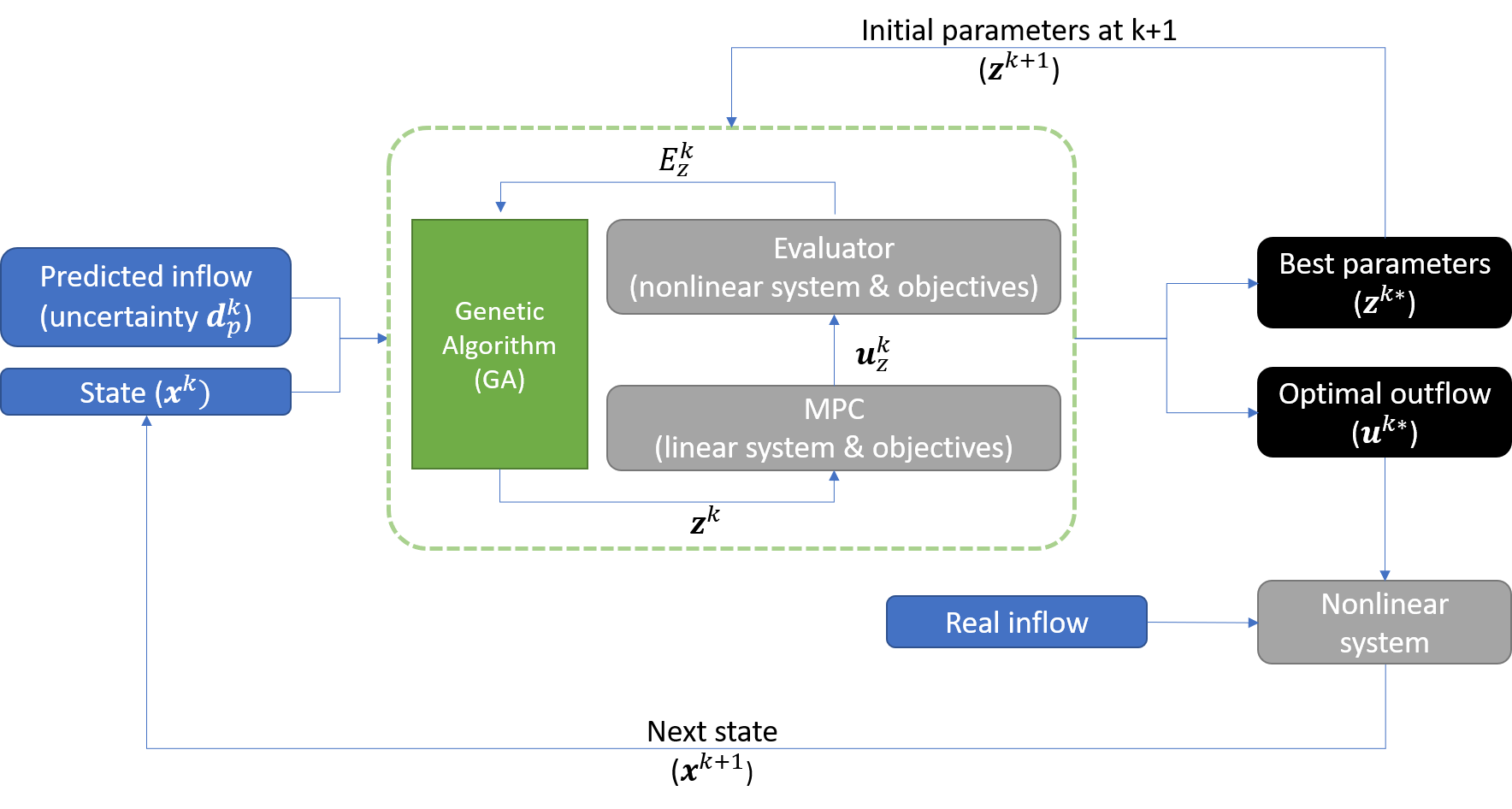
Figure 1: The schematic diagram of PD-MPC approach, with GA parameter $\mathbf{z}^{k}$ warm started with previous step optimal values.

Complex optimisation problems can be effectively tackled by gradient-free randomized search algorithms, like evolutionary and Genetic algorithms and Bayesian optimisation algorithms. We have selected the GA. The Genetic Algorithm is one of the most prominent and easy-to-implement gradient-free algorithms which imitate the natural selection process (see e.g., [20]). It continuously develops the population (a set of vectors seen as potential solutions) over each iteration, employing reproduction, crossover, and mutation operators, aiming at preserving the vectors with lower values of objective function, and iteratively recombining them.

As Figure 1 shows, GA explores the weight/parameter space to find a weight/parameter set with the lowest penalty from the evaluator at each time step. The optimal outflows for a prediction horizon are then computed based on this weight/parameter set. As the MPC horizon recedes, the first outflow is implemented, and the whole process is repeated with an updated state and newly predicted inflow. The disturbance, denoted as $\mathbf{d}_{p}^{k}$, represents a vector of the uncertainty of inflow at time step $k$, i.e. for time $k$ to $k+H-1$, where $H$ is the length of the prediction horizon. The state vector at time step $k$ is denoted as $\mathbf{x}^{k}$.

Control inputs have often been evaluated based on a single criterion, such as the possibility for system failure ([11]) or minimizing the worst-case impact ([42]). However, such approaches might overlook distinctions among control inputs concerning the operator’s preferences. For example, there may be no differentiation between maintaining outflow and increasing outflow in terms of the risk of system failure when RWL is still low. In this research, we employ all proposed practical objectives as evaluation criteria, through the use of the simulation-based Genetic Algorithm (GA), without limiting ourselves to linear and nonlinear objectives that are straightforward to implement in mathematical optimisation. This allows the PD-MPC framework, primarily optimising a linear MPC problem, to select an outflow schedule that actively aligns with the operator’s preferences. In the Evaluator, the objectives from $\tilde{J1}$ to $\tilde{J5}$, which are applied in the MPC formulation in linearised forms, are reformulated into non-linear equations, leveraging exponential functions to normalise all penalties. The evaluator also incorporates $\tilde{J6}$, $\tilde{J7}$, and $\tilde{J8}$, which aim to maintain the continuity of spillway gate conditions, to ensure that the outflow remains below the peak inflow up to the current time step, and to confirm full utilisation of turbine capacity before opening spillway gates, respectively (see Section 2.1). This is motivated by the difficulty of linearising $\tilde{J6}$ and $\tilde{J8}$, and the similarity of $\tilde{J7}$ to $\tilde{J1}$, which focuses on minimizing the peak outflow. The evaluator uses a nonlinear system simulation (i.e. nonlinear height-volume curve) to calculate water levels.

There are a few distinctions between the objectives outlined in Section 2.1 and those implemented in the evaluator. Specifically, for $\tilde{J3}$ and $\tilde{J4}$, the evaluator penalizes only increases, in contrast to the MPC formulation, which penalizes both increases and decreases. Regarding $\tilde{J5}$, direct application of $S_{H}$ is not feasible in PD-MPC due to its potential variability. Instead, two alternatives are introduced: penalizing instances where RWL increases within a prediction horizon and/or approaches FWL closely. For detailed explanations, including formulas, please refer to Appendix A.

3 Numerical Experiment

3.1 Description of the case study area

The Daecheong reservoir is located in the middle of South Korea, within the upper basin of the Geum river, as illustrated in Figure 2. There is another multipurpose reservoir, the Yongdam reservoir, located in the upper basin of the Daecheong reservoir. The outflows from the Yongdam reservoir have a direct influence on the flood control strategies of the Daecheong reservoir since they enter the Daecheong reservoir basin directly. Usually and understandably, operators decide the outflows of the Yongdam reservoir first, followed by decisions on the outflows of the Daecheong reservoir. Therefore, we assume that we have prior knowledge of the future outflows from the Yongdam reservoir. The specifications of the Daecheong reservoir are presented in Table 1.

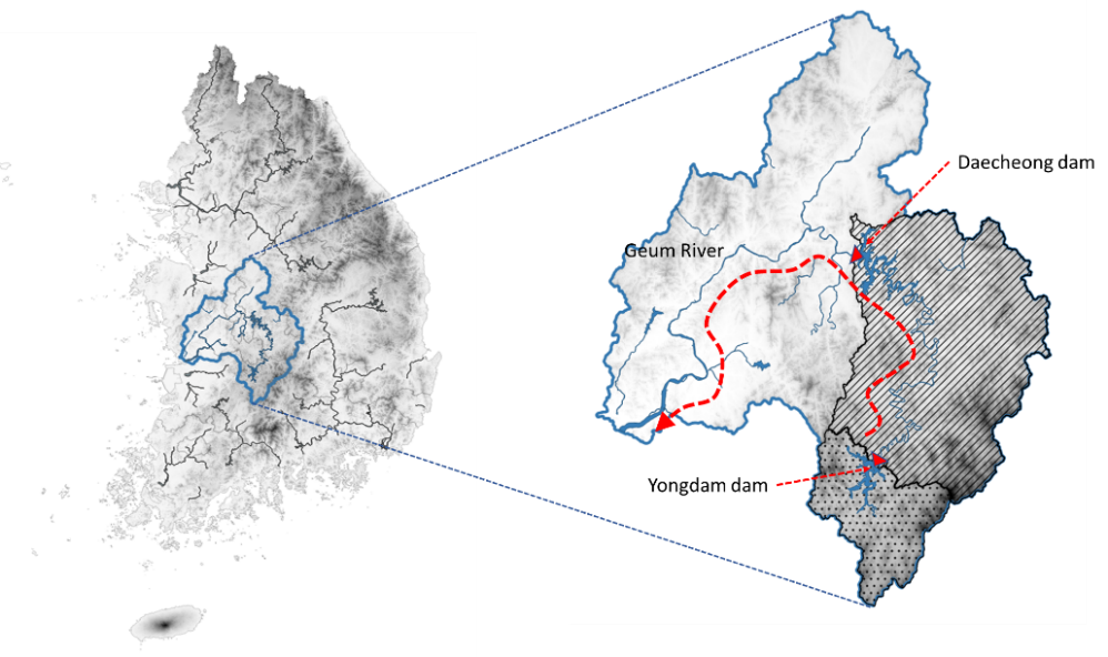
Figure 2: The Daecheong reservoir and Geum river basin.

Table 1: Specifications of the Daecheong reservoir.

FWL	EL. 80.0m	Total storage	1,490 $10^{6}m^{3}$
NHWL	EL. 76.5m	Spillway capacity	11,680 $m^{3}/s$
LWL	EL. 60.0m	Turbine capacity	264 $m^{3}/s$
Spillway crest level	EL. 64.5m	200yr Frequency Flood	10,700 $m^{3}/s$

The Daecheong reservoir has enough spillway capacity with the spillway crest level significantly lower than NHWL. The outflow capacity at NHWL is greater than 6,000 $m^{3}/s$, so we do not need to consider the spillway outflow capacity according to RWL. However, the flood control storage is relatively small. For example, the 200-year frequency inflow is 10,700 $m^{3}/s$, and it takes only 6.5 hours to completely fill the flood control storage. In addition, there is no restricted water level for the flood season in this reservoir. In essence, the Daecheong reservoir is susceptible to flooding, necessitating rapid and well-informed flood control decisions by operators to avert extreme conditions.

Three flood events with a large amount of peak inflow and one to three peaks are selected from historical data as presented in Table 2. To the best of our knowledge, most studies have primarily concentrated on floods lasting one to two days ([38, 6, 13]). In the case of short flood events, generating reliable outflows is relatively straightforward because the trade-offs among objectives are evident. For instance, it is clear that minimising outflows leads to an increase in reservoir water level, and vice versa. However, the situation becomes more complex over longer time frames. Minimising outflows can ironically result in increased outflows if peak inflow occurs after the reservoir water level has already risen significantly. Therefore, our research examines floods lasting at least three days, featuring one to three peaks, to provide a more practical case study.

Table 2: Study flood events.

Periods	Duration	Peak inflow	Feature
from 2 July 2016 to 11 July 2016	197 hour	3,655 $m^{3}/s$	Double peak
from 25 August 2018 to 7 September 2018	311 hour	2,590 $m^{3}/s$	Triple peak
from 1 September 2020 to 12 September 2020	269 hour	4,468 $m^{3}/s$	One peak

To simulate the uncertainty associated with inflow predictions, we generate ‘predicted’ inflow data by multiplying random numbers by real inflow, as Equation (8). Predicted inflow should be positive, and random numbers are generated by a normal distribution with a mean of zero and a standard deviation of $a$. The predicted inflow could be negative due to a normal distribution; therefore, the lower boundary $c$ is introduced. Typically, forecasting uncertainty tends to increase as the forecast period increases. To reflect this, we adjust the standard deviation by increasing it by $b$ per each time step. Moreover, a moving average filter with a three-hour window is applied at every time step. This filter helps prevent unreasonable high fluctuations in predicted inflow within the prediction horizon.

$$\begin{split}PI_{t}&=\frac{1}{3}\sum_{j=t-2}^{t}RI_{j}\times\omega I_{t},\\ &\omega I_{t}=\begin{cases}1+x\text{, where }\sim\mathcal{N}(0,(a+T\times b)^{2})&\text{if }1+x\geq c,\\ c&\text{otherwise,}\end{cases}\end{split}$$ (8)

where $PI_{t}$ and $RI_{t}$ are the predicted and real inflow at time $t$, while $\omega I_{t}$ denotes the uncertainty of inflow at time $t$. $T$ is the order of forecasting time within a prediction horizon to increase prediction uncertainty for a longer time. $a$, $b$, and $c$ are set as 0.05, 0.03, and 0.1 arbitrary. The sample hydrographs of real and predicted inflow are provided in Appendix B.

3.2 A reservoir flood control system

3.2.1 System model

A simple linear reservoir model can be expressed as

$$S_{t+1}=S_{t}+I_{t}-O_{total,t},$$ (9)

where $S_{t}$ is the current storage of a reservoir at time $t$, and $I_{t}$ and $O_{t}$ are the total amount of inflow and outflow for time $t$, respectively. Errors in measuring water level, calculating storage amount and outflow are not considered for simplification. In addition, evaporation and seepages are also not explicitly considered in Equation (9), but these factors are already accounted for in the inflow data. This is because inflow is not directly measured but calculated using Equation (9) from measured outflow and storage timeseries for the Daecheong reservoir.

3.2.2 Constraints

The operational constraints can be formulated as follows:

(1) The total outflow is more than the sum of the agreed amounts with water users and the in-stream flow, i.e. the downstream demand:

$$D_{t}\leq O_{total,t},$$

where $O_{total,t}$ and $D_{t}$ are the total outflows and the downstream demand at time $t$, respectively.

(2) RWL should be between FWL and LWL:

$$\text{LWS}\leq S_{t}\leq\text{FWS},$$

where $S_{t}$ is the reservoir storage at time $t$, while LWS and FWS are the reservoir storage at Low Water Level (LWL)and Flood Water Level (FWL), respectively.

(3) Outflows via the turbine and spillway gates are not able to exceed their capacity:

$$\begin{split}&O_{turb,t}\leq MO_{turb},\\ &O_{spill,t}\leq MO_{spill},\end{split}$$

where $O_{turb,t}$ and $O_{spill,t}$ represent the turbine and spillway outflow at time $t$, respectively. $MO_{turb}$ and $MO_{spill}$ are the outflow capacity of turbines and spillway gates. We take into account the spillway crest level in our analysis, but spillway outflow capacity based on RWL is disregarded as explained in Section 3.1.

3.2.3 Objectives

By reflecting the practical objectives described in Section 2, the objective function of MPC is set as below:

$$\min J1^{k}+J2^{k}+J3^{k}+J4^{k}+J5^{k},\\$$ (10)

where,

$$\begin{split}J1^{k}&\coloneqq\max_{t\in k,\ldots,k+H-1}O_{spill,t}^{k}\times w_{1},\\ J2^{k}&\coloneqq\sum_{t=k}^{k+H-1}O_{spill,t}^{k}\times w_{2},\\ J3^{k}&\coloneqq\sum_{t=k+1}^{k+H-1}\delta O_{t}^{in,I}\times w_{3,I}+\delta O_{t}^{in,D}\times w_{3,D},\\ J4^{k}&\coloneqq\sum_{t=k}^{k+H-1}\delta O_{t}^{between,I}\times w_{4,I}+\delta Q_{t}^{between,D}\times w_{4,D},\\ J5^{k}&\coloneqq\sum_{t=k}^{k+H-1}\mu S_{t}^{1}\times w_{5,1}+\mu S_{t}^{2}\times w_{5,2}+\mu S_{t}^{3}\times w_{5,3},\end{split}$$ (11)

subject to,

$$O_{spill,t}^{k}+O_{turb,t}^{k}-O_{total,t}^{k} =0,$$

$$O_{total,k}^{k}-O_{total,k}^{k-1} =0,$$ (12)

$$\delta O_{t}^{in,I}-\delta O_{t}^{in,D}+(O_{total,t}^{k}-O_{total,t-1}^{k})\times w_{\delta O_{in,t}} =0,$$

$$\delta O_{t}^{between,I}-\delta O_{t}^{between,D}+(O_{total,t}^{k}-O_{total,t}^{k-1})\times w_{\delta O_{between,t}} =0,$$ (13)

$$\mu S_{t}^{1}+S_{U}-S_{t} \geq 0,$$

$$\mu S_{t}^{2}+S_{t}-S_{L} \geq 0,$$

$$\mu S_{t}^{3}+S_{H}-S_{t} \geq 0,$$ (14)

$$\delta O_{t}^{in,I}\text{, }\delta O_{t}^{in,D}\text{, }\delta O_{t}^{between,I}\text{, }\delta O_{t}^{between,D}\text{, }\mu S_{t}^{1}\text{, }\mu S_{t}^{2}\text{, }\mu S_{t}^{3} \geq 0,$$

where $J_{1}^{k}$, for example, is an objective for the MPC formulation at time step $k$. All objectives are multiplied by their respective weights and then summed together to form the objective function, as shown in Equation (10) and (11). Weights, i.e. $w_{1}$, $w_{2}$, $w_{3,I}$, $w_{3,D}$, $w_{4,I}$, $w_{4,D}$, $w_{5,1}$, $w_{5,2}$, and $w_{5,3}$, are multiplied by each objective.

Several positive slack variables are introduced to linearise objectives instead of applying absolute forms. These variables include $\delta O_{t}^{in,I}$ and $\delta O_{t}^{in,D}$, representing the step-wise increase and decrease in outflows in a prediction horizon; $\delta O_{t}^{between,I}$ and $\delta O_{t}^{between,D}$, representing the increase and decrease in outflow schedules at time step $k$ and $k-1$; $\mu S_{t}^{1}$, $\mu S_{t}^{2}$, and $\mu S_{t}^{3}$, representing the storage violation above $S_{U}$, below $S_{L}$ and above $S_{H}$, respectively. To account for varying penalties over time, we assign weights $w_{\delta O_{in,t}}$ and $w_{\delta O_{between,t}}$ to each change at time $t$. The idea is to penalise changes closer to the start of the horizon more than changes farther ahead in the horizon. In this work, we set $w_{\delta O_{in,t}}$ to $\frac{1}{(t-k+1)\times 3}$, and $w_{\delta O_{between,t}}$ is set as follows:

$$\begin{split}w_{\delta O_{between,t}}=\begin{cases}\frac{1}{t-k+1}&\text{if }t\leq k+3,\\ \frac{1}{(t-k+1)\times 2}&\text{otherwise.}\end{cases}\end{split}$$

The target water levels, such as $S_{U}$ and $S_{L}$, are defined as mentioned in Section 2.1. The weights of objectives in Equation (11), as well as the allowed highest water level, $S_{H}$ in Equation (14), will be found during the optimisation process.

The important difference in the objective formulas presented in Section 2.1 is about $O_{total,k}^{k}$ in Equation (12) and $\tilde{J4}$ in Equation (2). Note that $O_{total,k}^{k}$ is the first outflow in the optimal control inputs at time step $k$. First, changing the outflow for time $k$ at time step $k$ is practically impossible because it involves implementing the current outflow while calculating it. To address this, we separate this to ensure it, rather than assigning significant weight to the change in the first outflow in Equation (13). Hereby, the outflow decision is delayed for a time step.

3.3 PD-MPC design

Since the Korea Meteorological Agency (KMA) publishes $6$-hour quantitative rainfall forecasts every hour, in the experiment, we employed four different prediction horizons: $6$, $12$, $18$ and $24$ hours. Starting from the 6 hours, the longer horizons allow us to explore the effect of horizon length on performance. The control horizon is the same as the prediction horizon. For the initial run at $t=0$, we set the initial storage to the corresponding level of NHWL (EL. $76.5m$), while the initial outflows via the turbines and spillway gates are set to 150 $m^{3}/s$, which is the average hourly outflow during the flood season from 2015 to 2020, and 0 $m^{3}/s$, respectively.

In this experiment, the GA optimises $10$ parameters, comprising of $9$ weights for the objectives and $1$ parameter for the highest RWL, denoted as $S_{H}$. To reduce the running time of GA, we impose search range limits for each weight and parameter, as outlined in Table 3. In $J5$ in Equation (11), $w_{5,2}$ and $w_{5,3}$ are fixed at twice and twenty times of $w_{5,1}$, respectively, because maintaining RWL under $S_{H}$ for dam safety is a higher priority than maintaining it between target levels. Therefore, the number of weights and parameters explored becomes $8$ from $10$. All weights share the same length of the search range, except for $J2$. This is because the weight of $J2$, i.e. minimising the total outflows via spillway gates, can be relatively small due to its similarity to $J1$, i.e. minimising the peak outflows via spillway gates, and we want to emphasize $J1$. To ensure $J5$ is not neglected, the search ranges for $w_{5,1}$, $w_{5,2}$, and $w_{5,3}$ start from $1$, not from $0$. Moreover, to scale all weights and facilitate GA exploration within integer space, we introduce multipliers based on the MAVE of each objective. Therefore, each weight is calculated by multiplying a selected value within the search range by its respective multiplier.

We prepare MPC baselines with fixed weights and a fixed parameter set, denoted as ‘Fixed’. To ensure the feasibility of the problem, two weight/parameter sets are selected from the best weight/parameter sets generated from various PD-MPC tests. Throughout this paper, we refer to the value before being multiplied by the multiplier as the weights unless this would cause confusion otherwise.

Table 3: The possible range for PD-MPC and fixed weights/parameters for the baseline MPC.

P	$w_{1}$	$w_{2}$	$w_{3,I}$	$w_{3,D}$	$w_{4,I}$	$w_{4,D}$	$w_{5,1}$	$w_{5,2}$	$w_{5,3}$	$S_{H}$
Multiplier	$\frac{20}{MO_{s}pill}$	$\frac{2}{MO_{s}pill}$	$\frac{20}{MO_{s}pill}$	$\frac{20}{MO_{s}pill}$	$\frac{20}{MO_{s}pill}$	$\frac{20}{MO_{s}pill}$	$\frac{20}{FWS\times F}$	$\frac{40}{FWS\times F}$	$\frac{400}{FWS\times F}$	-
Search range	0-19	0-2	0-19	0-19	0-19	0-19	1-20	$\leftarrow$	$\leftarrow$	$RWS$
Fixed-1	3	1	3	3	20	20	15	$\leftarrow$	$\leftarrow$	$RWS_{F}$
Fixed-2	20	5	3	3	3	3	15	$\leftarrow$	$\leftarrow$	$RWS_{F}$

In Table 3, a searching range of $S_{H}$ is the storage where RWL is in $\{$EL. 78.5m, 79.0, 79.5m$\}$ and $S_{H}$ of the baselines, i.e. $RWS_{F}$ (Reservoir Water Storage for Fixed weights/parameter set), which is the stored amount of water at EL.79.0m. A computer code is developed using Python. In detail, pyomo ([16]), GLPK solver ([27]) and pyGAD ([14]) packages were applied to implement the numerical experiment of PD-MPC.

4 Results and discussion

4.1 PD-MPC results

Parameterised Dynamic Model Predictive Control (PD-MPC)delivers reliable results across all events and prediction horizons. The results show only a few changes in outflow schedules, and all peak outflows remain below the peak inflow. RWL consistently is between $S_{H}$ and $S_{L}$. As expected, the performance of MPC under certainty generally surpasses the results obtained under uncertainty. Peak outflows and RWL s from uncertain inflow exceed those from certain inflow, and the reservoir should change the outflow schedule more often. Detailed experimental results are available in Appendix C.

The performance of this framework can be presented clearly when compared to the Fixed cases, as shown in Figure 3 under uncertain inflow. Different symbols in the figure represent different prediction horizons: 6, 12, 18, and 24 hours. The Fixed-1 case assigns relatively high weights to minimise the changes in outflow schedules, while the Fixed-2 case prioritizes minimising peak outflow. The results challenge our expectations. The Fixed cases do not consistently outperform PD-MPC, even in their main targets. It is impossible to assert that the Fixed-1 case is always superior to the other two cases concerning the changes in outflow schedules, as shown in Figure 3(a) and 3(d). Similarly, peak outflows of the Fixed-2 case are not certainly less than the other two cases, as demonstrated in Figure 3(b) and 3(e). This suggests that stationary weights fail to consistently represent the operators’ preference. This can be attributed to the complexity of trade-offs for each time step and the relatively shorter prediction horizon length compared to the length of a flood event. For example, we often assume that a lower peak outflow leads to a higher peak RWL. However, the results show that this assumption does not always hold true, as demonstrated in Figure 3(c) and 3(f). This is because the myopic outlook on optimal outflows at each time step could lead to suboptimal outcomes when viewed in the context of the entire flood event. In our case, the evaluator effectively makes MPC have a long-term perspective compared to the Fixed cases. In addition, we can observe that PD-MPC utilized the storage capacity more effectively than the Fixed cases.

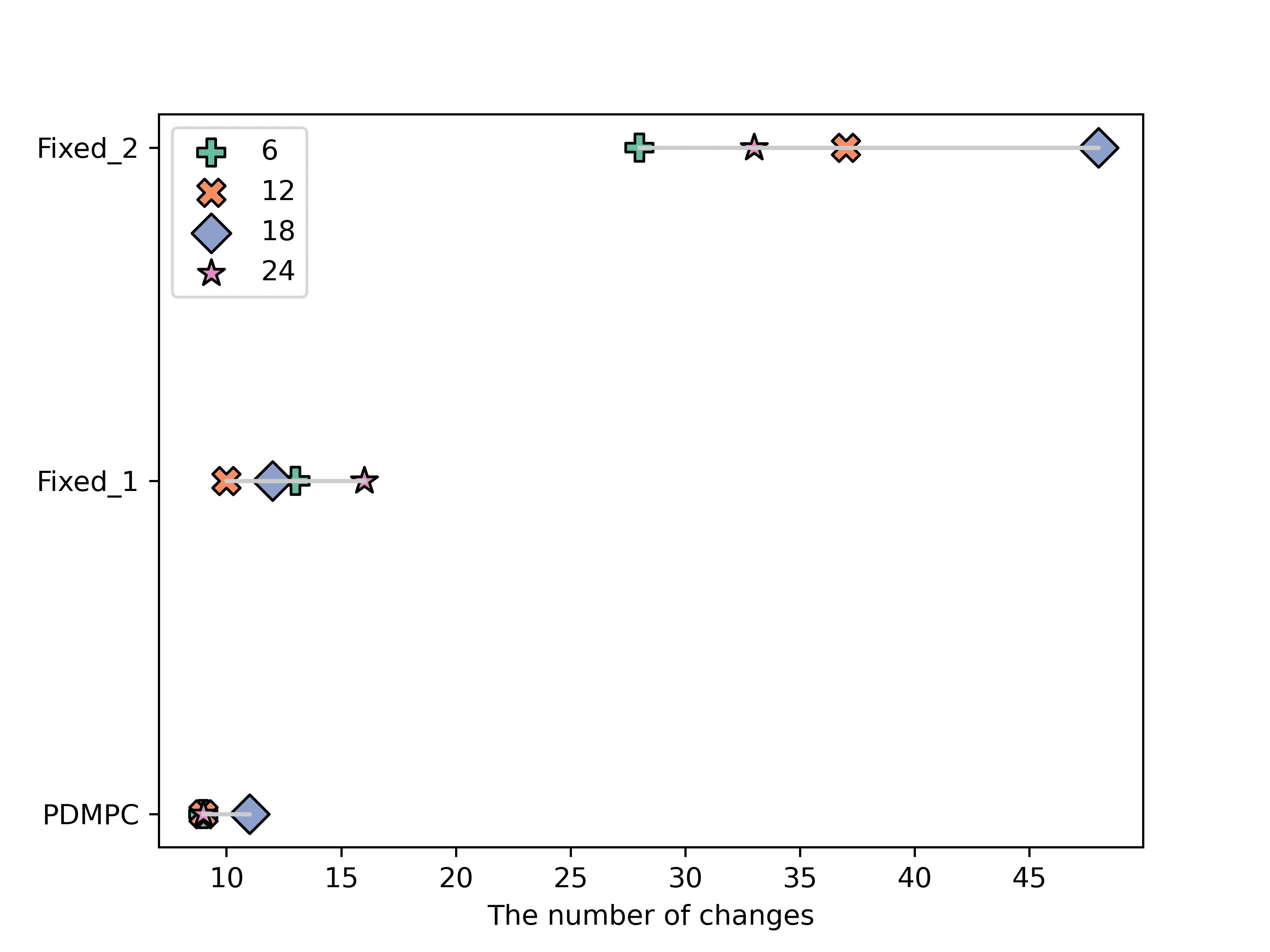
(a)

(b)

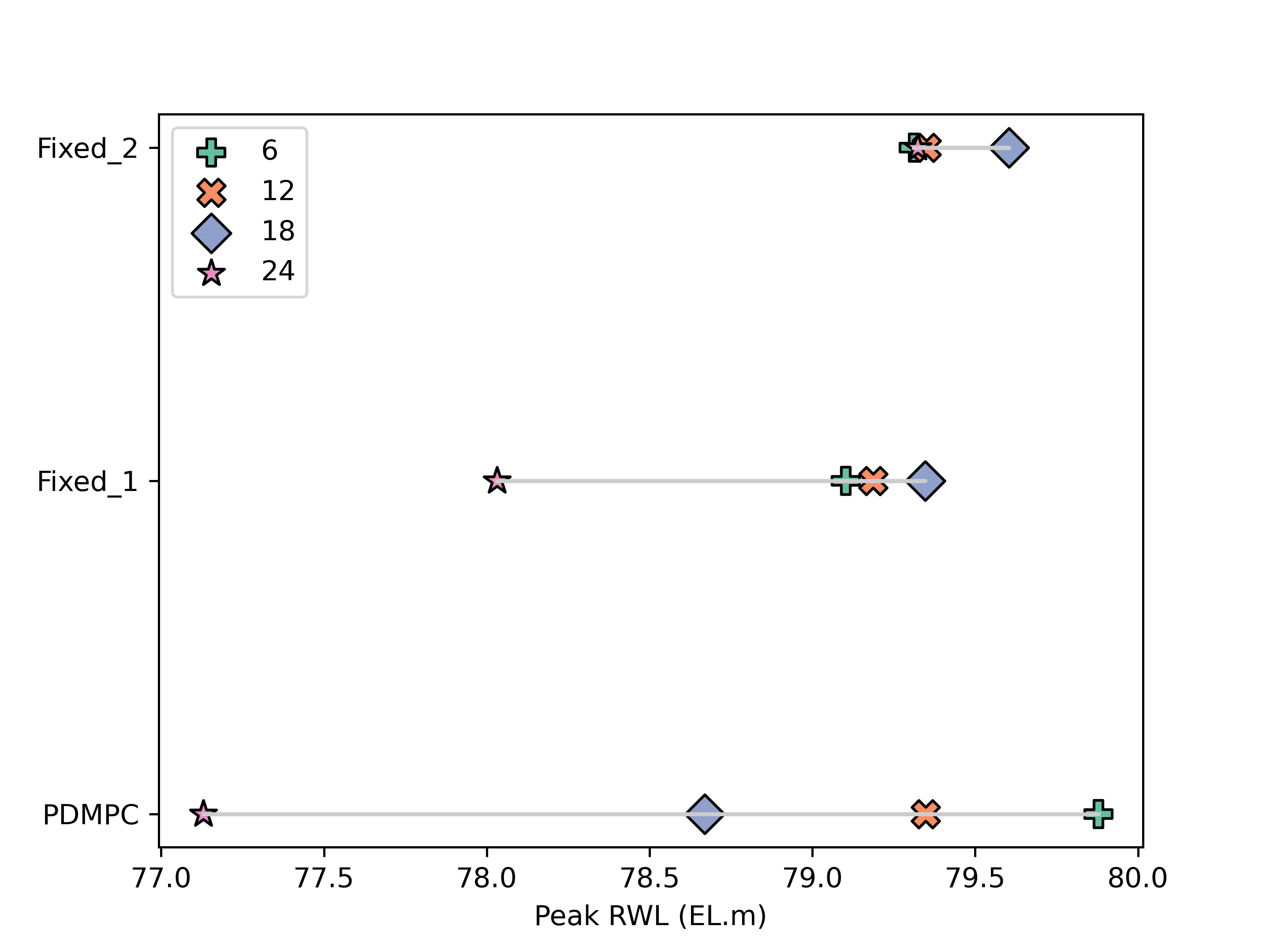
(c)

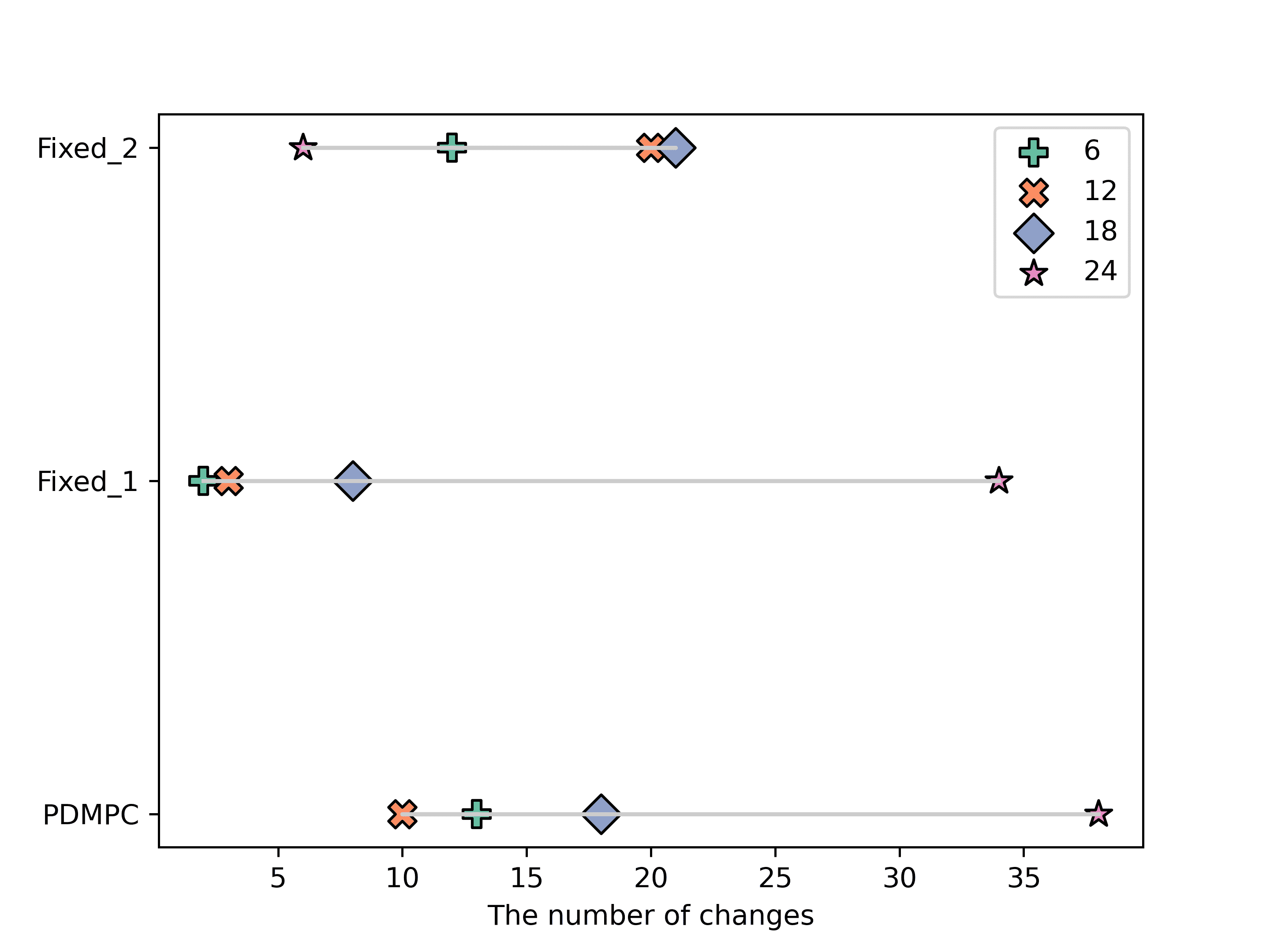
(d)

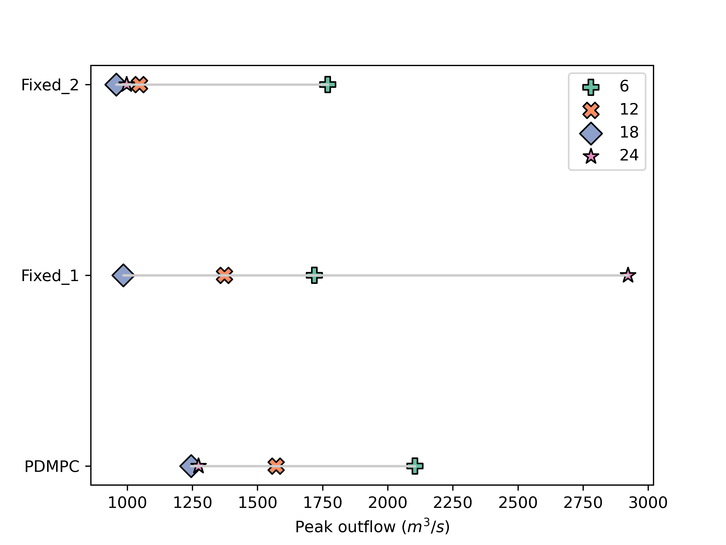
(e)

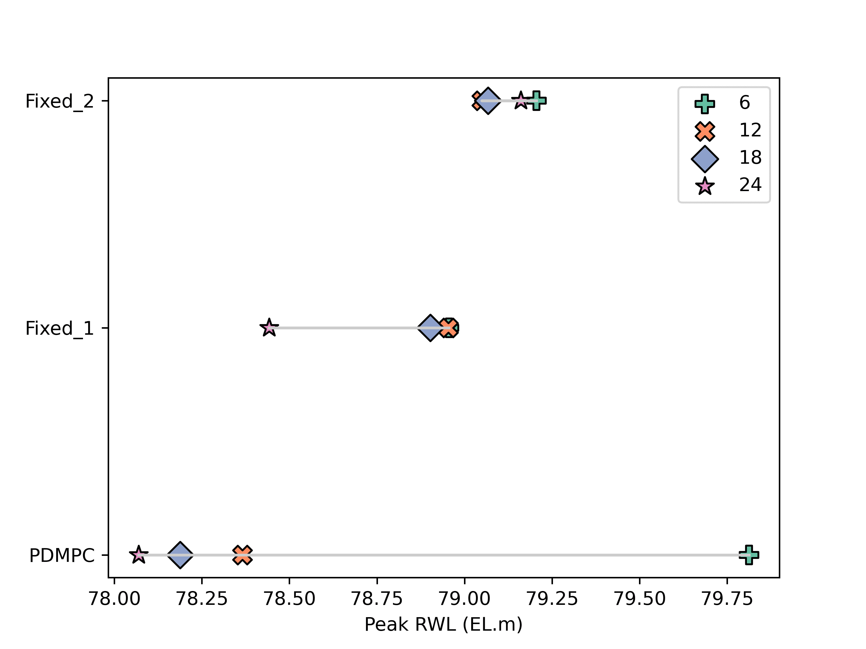
(f)

Figure 3: Comparison with the Fixed cases under uncertain inflow. (3(a)) The number of changes between consecutive outflow schedules for Event 1. (3(b)) Peak outflow for Event 1. (3(c)) Peak RWL for Event 1. (3(d)) The number of changes between consecutive outflow schedules for Event 3. (3(e)) Peak outflow for Event 3. (3(f)) Peak RWL for Event 3.

In Figure 4, the maximum penalty value of PD-MPC is less than 20 in any case. We have high penalty values above 1,000 when $\tilde{J7}$, which penalises when the peak outflow exceeds the maximum inflow up to the current time steps, is active or RWL is approaching FWL. Notably, both Fixed cases exhibit these undesirable conditions many times, contrary to the fact that it has never occurred in PD-MPC.

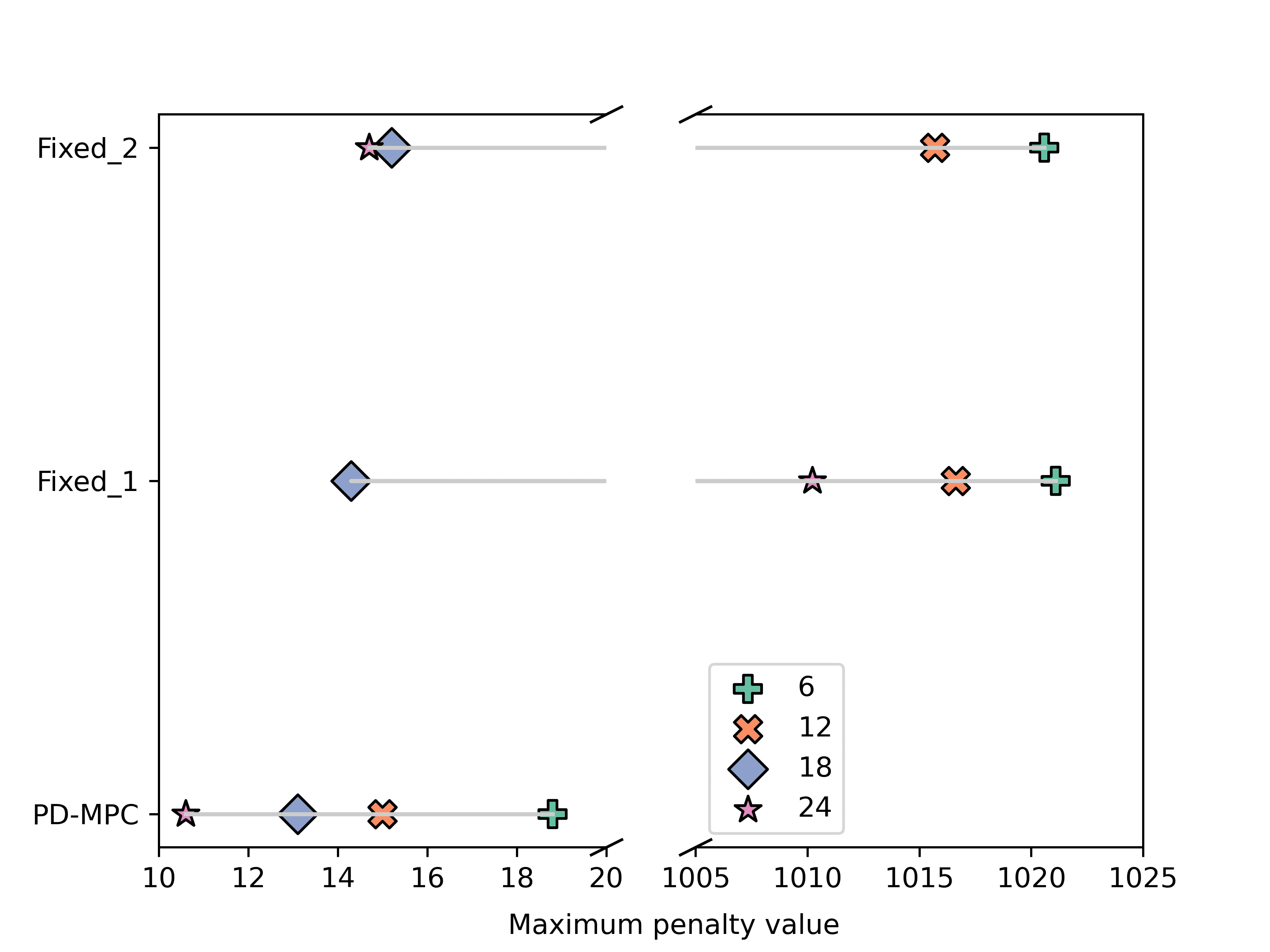
(a)

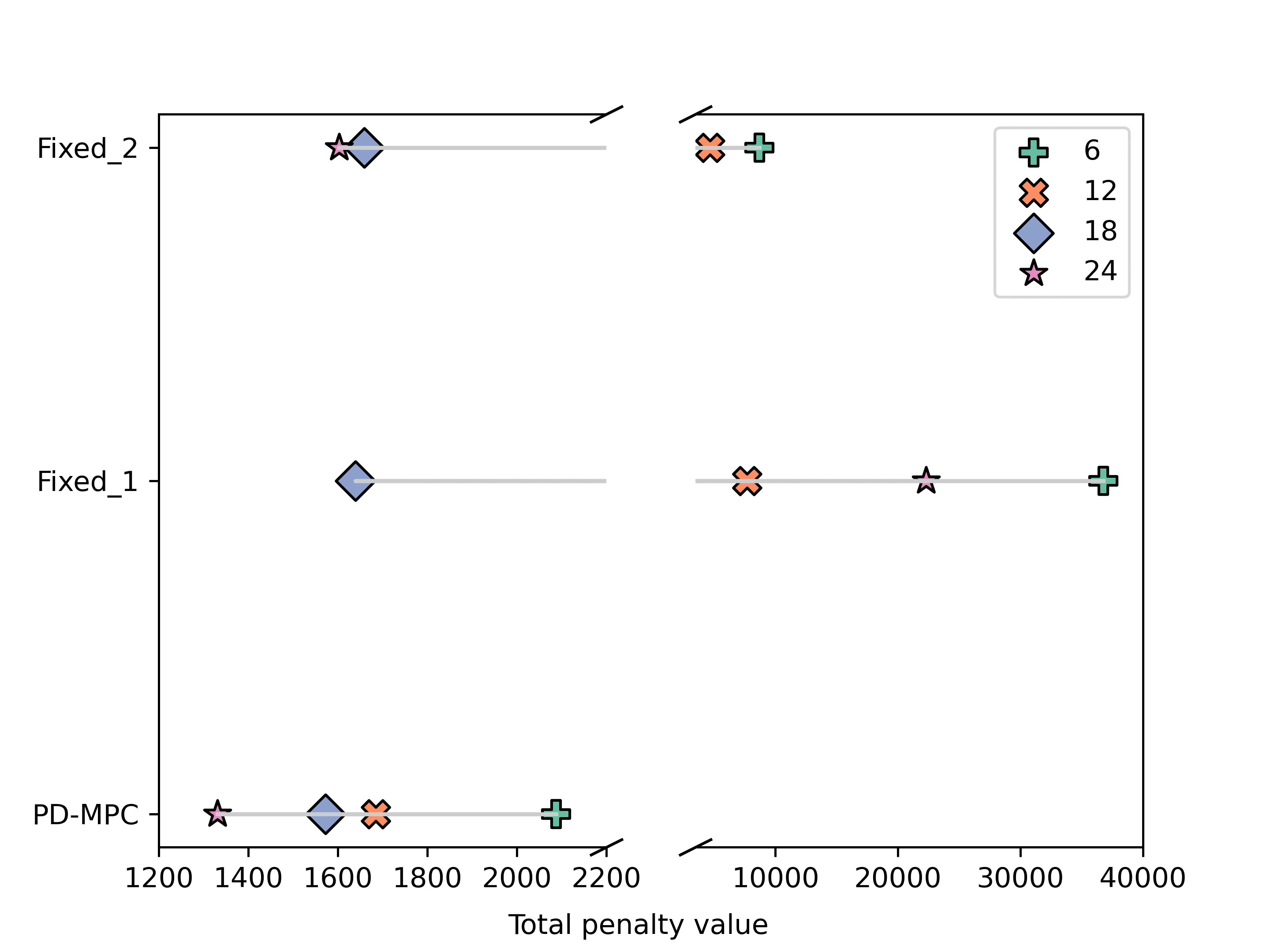
(b)

Figure 4: The penalty values from the evaluator for Event 1 under uncertain inflow. (4(a)) The maximum penalty. (4(b)) The total penalty (sum of penalty values).

To see the impact of the evaluator, we systematically adjusted the importance of the changes in outflows calculated at consecutive time steps and compared it with the previous one. The result is straightforward. When the evaluator assigns a higher weight to $\tilde{J4}$, it leads to fewer changes in outflows but comes at the expense of peak outflow and RWL. For detailed results, please refer to Appendix C. PD-MPC with the low $\tilde{J4}$ case shows a greater number of changes. Given the unambiguous response from PD-MPC, it can be inferred that the evaluator effectively affects the selection of the optimal weight/parameter set.

4.2 Parameters as elements of operators’ preference

In Section 1, we discussed that some researchers had focused on finding appropriate weights when defining preferences in a multi-objective setting. To demonstrate the parameters should also be regarded as important components of the preference, we conducted an experiment for Event 1, where we fixed $S_{H}$ to the storage level at EL. 79.0m and compare it with the results of PD-MPC where $S_{H}$ is a dynamic parameter to be optimised.

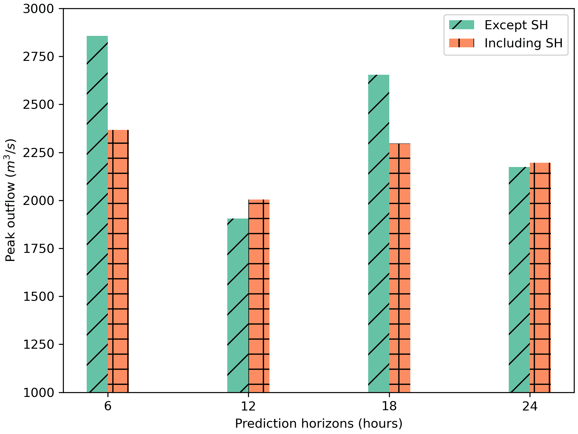
(a)

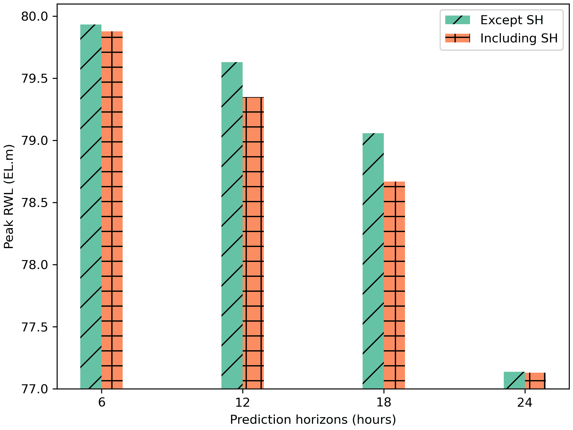
(b)

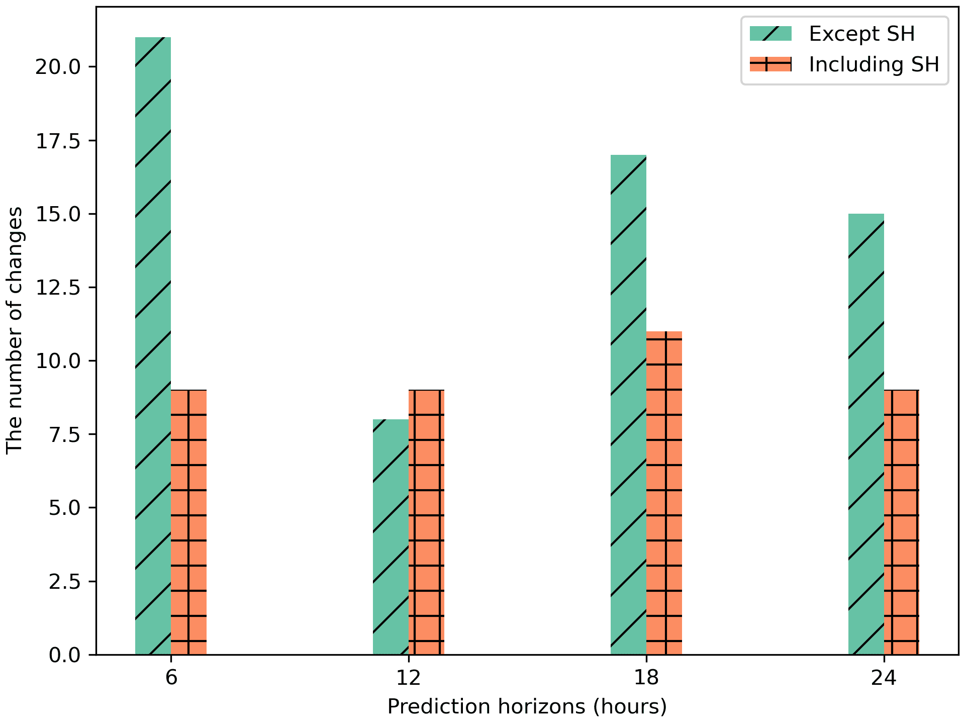
(c)

Figure 5: Comparison between the weight/parameter set including SH and excluding SH under uncertain inflow. (5(a)) Peak outflow. (5(b)) Peak RWL. (5(c)) The number of changes between consecutive outflow schedules.

PD-MPC, including the parameter $S_{H}$, outperforms PD-MPC with fixed $S_{H}$, which generally considers only the combination of weights as the representative of the preference, as illustrated in Figure 5. It seems reasonable to assume that operators would prefer the evaluator to have a lower $S_{H}$ because it results in a lower peak RWL. However, this is not the case because a lower $S_{H}$ can lead to a higher peak outflow. PD-MPC, by varying $S_{H}$, effectively achieves lower peak outflows and RWL s simultaneously. This means that an adaptively changing $S_{H}$ helps operators utilise the reservoir storage more efficiently. For instance, in PD-MPC with the parameter $S_{H}$, hydrological discharge tends to commence earlier compared to PD-MPC without $S_{H}$, achieved by maintaining a low $S_{H}$ before the water level rises significantly. Consequently, there is an impact on reducing both the peak outflow and the peak RWL. In addition, when RWL is close to $S_{H}$, and there is a sudden increase in inflow, fixing $S_{H}$ would result in a substantial and abrupt increase in outflow, even if there is some storage available between $S_{H}$ and FWL. In contrast, with adaptively changing $S_{H}$, PD-MPC chooses to increase $S_{H}$ to utilise the remaining storage, instead of resorting to a drastic and sudden increase in outflow.

4.3 The best weights/parameters can vary with time

In Section 2.2, we discussed the complexity of trade-offs among objectives, which led us to assume that the operator preferences among them can be dynamic. We can show this assumption in two ways. First, we found that the best weights/parameters varied with time steps. This is also true because the objectives that relate to violations of water levels, for example, have zero contributions to the weighted sum of all objectives unless some boundaries are exceeded and so depend dynamically on the system state. Since the best weights/parameters were determined through the optimisation process, we can say that the preference needs to be considered dynamic. Due to this variation, the objective values also fluctuate substantially. The fluctuation of objective values and the best weight/parameter sets selected by the evaluator reflect the dynamic nature of the relationship, which is influenced by the current state, such as the current RWL, predicted inflow, and scheduled outflows.

Second, Figure 6 illustrates the variation in penalty values as a weight only for the objective function related to RWL ($J5$) changes within our search range, while other objectives’ weights are the same as the weights from PD-MPC. For example, when a weight value for the $J5$ is two, it denotes that $w_{5,1}$ is $2\times\frac{20}{FWS\times F}$, $w_{5,2}$ is $2\times\frac{40}{FWS\times F}$, and $w_{5,3}$ is $2\times\frac{400}{FWS\times F}$ (see Table 3). Bright colours in the figure represent relatively low penalty values. The value of $99$ in black colour does not mean the penalty is precisely 99, but the actual penalty is much higher. For simplification, we convert all high penalty values into $99$, which indicates undesirable conditions such as when the outflow exceeds the peak inflow up to the current time step or the RWL approaches FWL. Since the evaluator computes a nonlinear objective with nonlinear system simulations (see Figure 1), the same penalty values, which also mean the same control inputs, are observed in many cases for different weight sets. Despite that, it is evident that the best weight set changes at every time step. This dynamic nature of optimal weight sets underscores the need for a flexible and adaptable approach in reservoir flood control. In addition, it effectively conveys that the outputs from an MPC formulation with static weights can, at best, be equal to those obtained through PD-MPC.

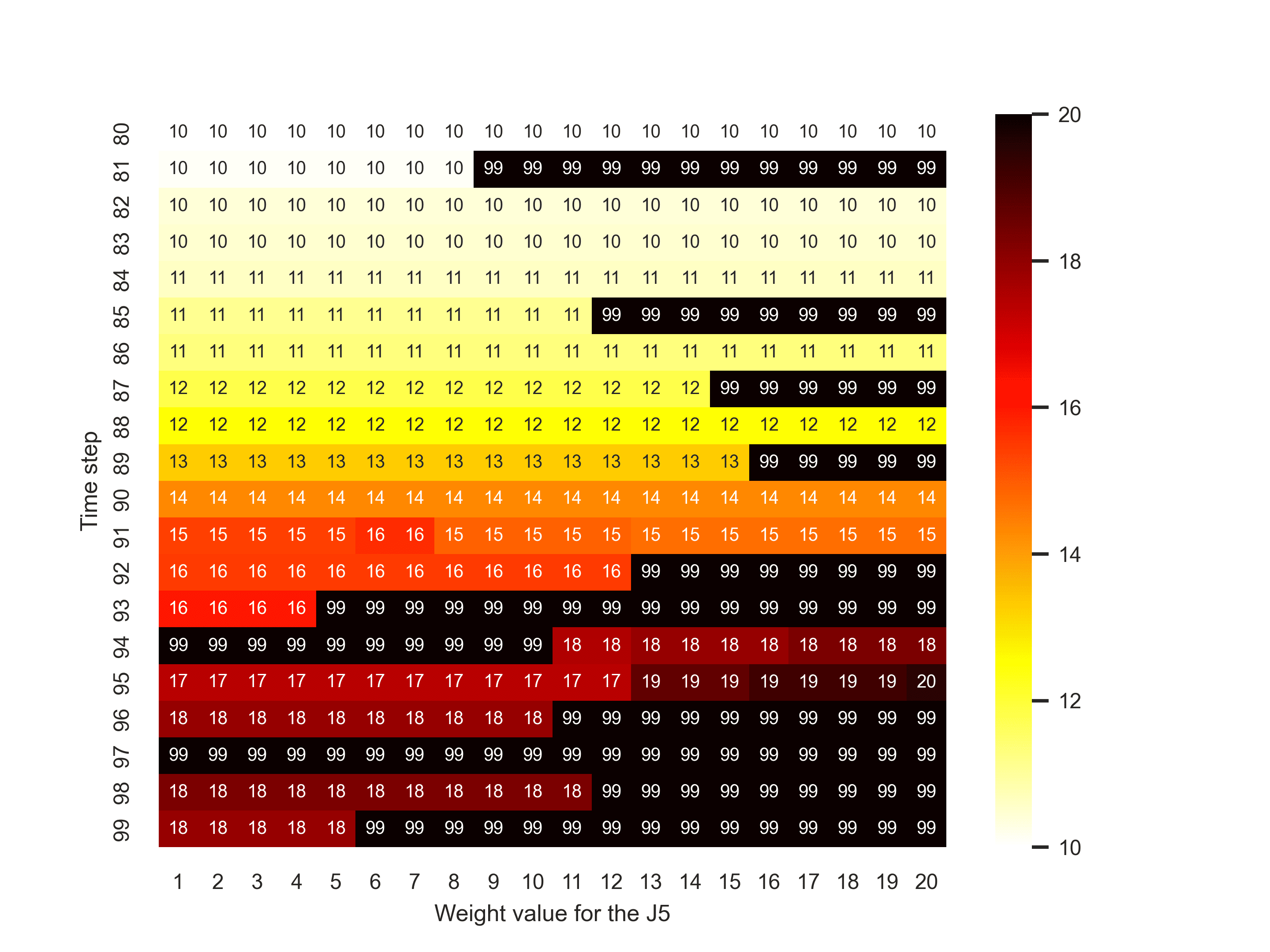
(a)

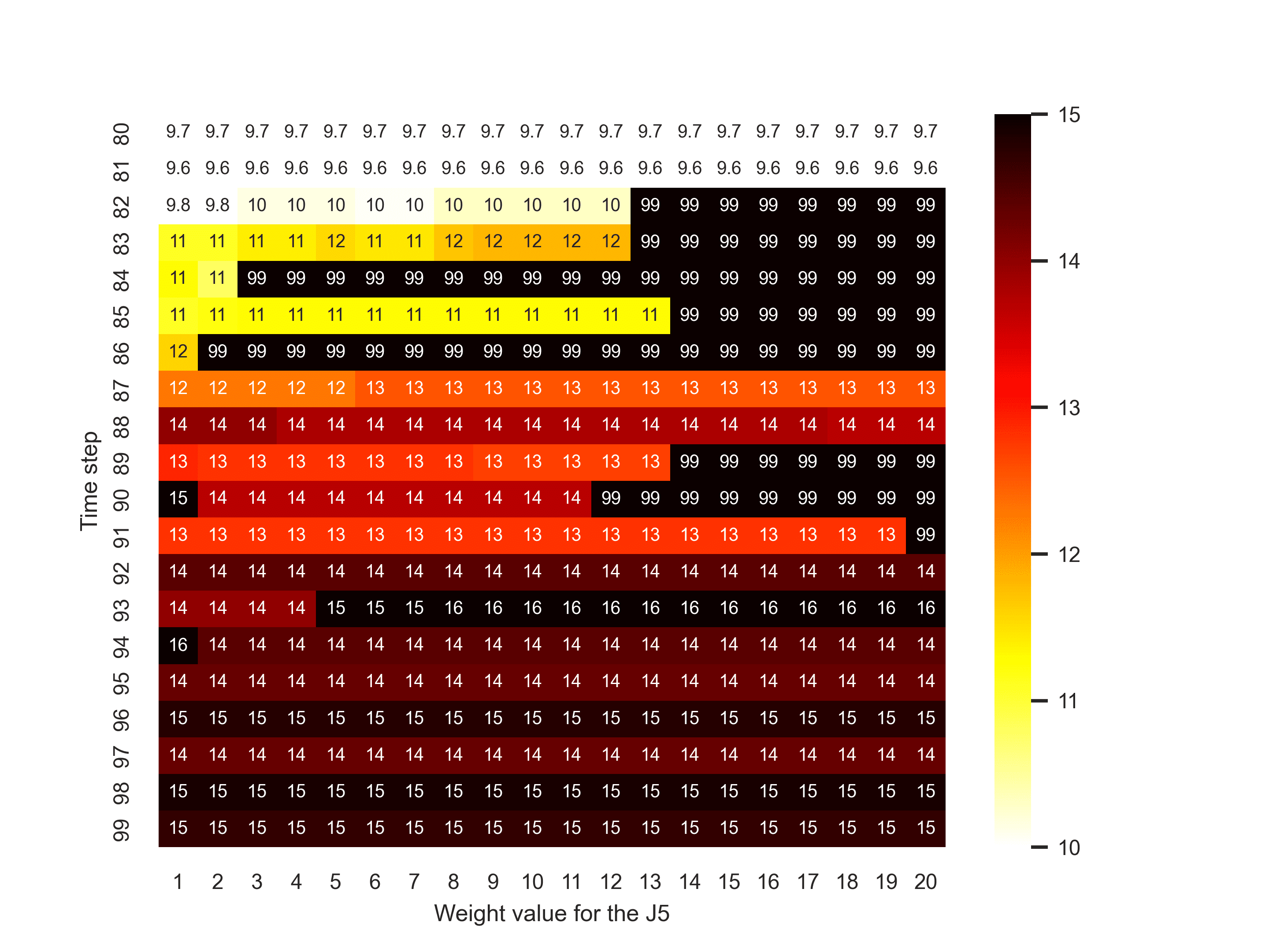
(b)

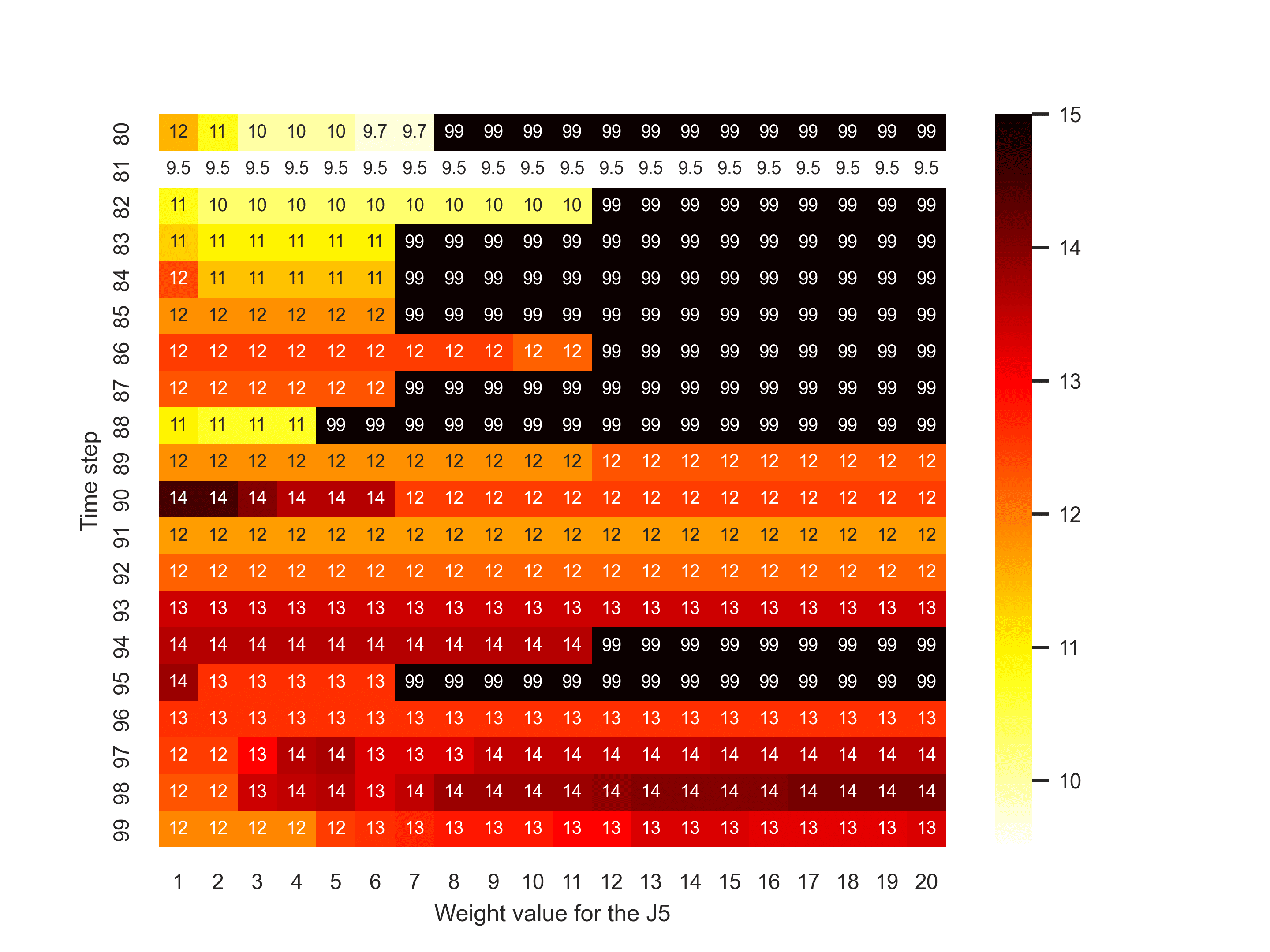
(c)

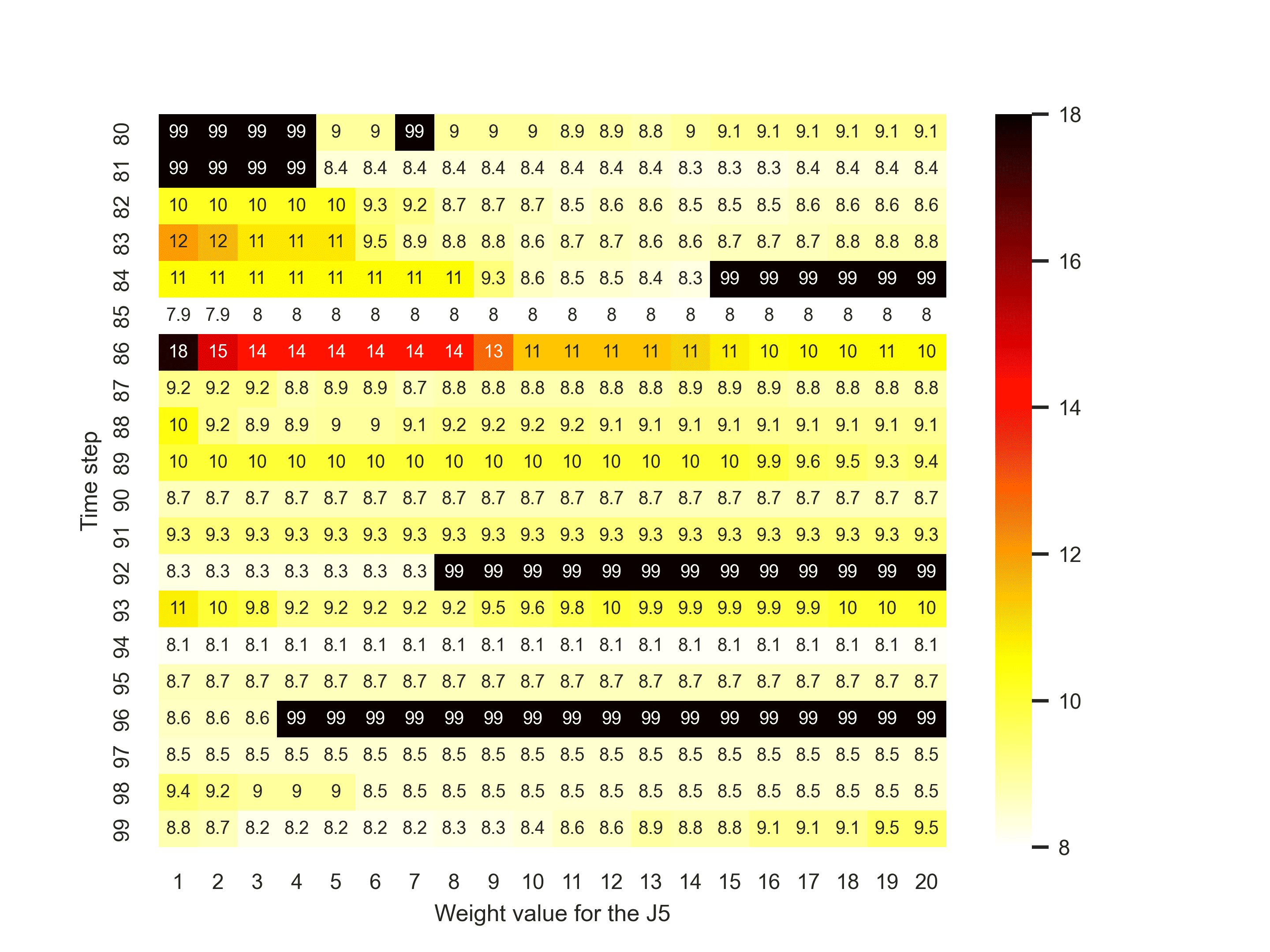
(d)

Figure 6: The colour represents the penalty value calculated at each time step from $k=80$ to $k=99$, with different weight values for the $J5$ while inflow increases steeply for Event 1. The prediction horizons are for: (6(a)) $6$ hours. (6(b)) $12$ hours. (6(c)) $18$ hours. (6(d)) $24$ hours.

Third, the normalized objective values, i.e. objective values before multiplying the weights and scaled from 0 to 1, fluctuate at every time step. Figure 7 illustrates three cases: (a) before the flood begins, (b) when the flood inflow is around its peak, and (c) near the end of the flood. In the figure, seven different lines represent different weight sets, such as $J1$ = (1, 0, 0, 0, 0, 0, 0), $J4$ = (0, 0, 0, 0, 1, 1, 0), and so on. The ‘Equal’ line corresponds to (1, 1, 1, 1, 1, 1, 1), while the ‘Fixed 1’ and ‘Fixed 2’ mean the Fixed cases presented in Table 3. ‘PD-MPC’ indicates the weight set selected by a PD-MPC framework. Note that each weight set needs to be multiplied by the respective multiplier presented in Table 3 before applying it to MPC. The x-axis in the figure represents each objective. To simplify the illustration, the allowed highest water level, $S_{H}$, is fixed at the storage of EL.79.0m for all cases.

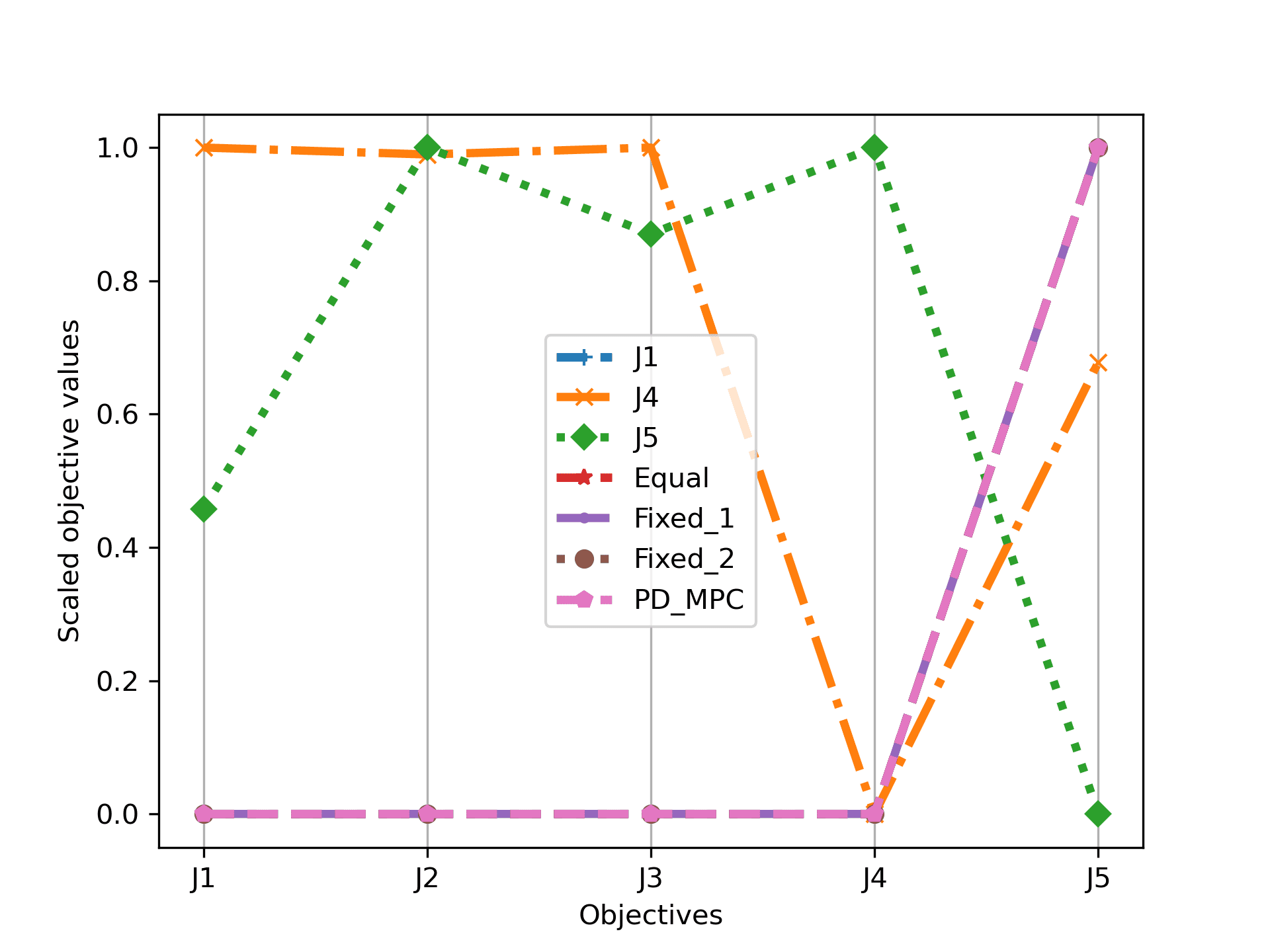
(a)

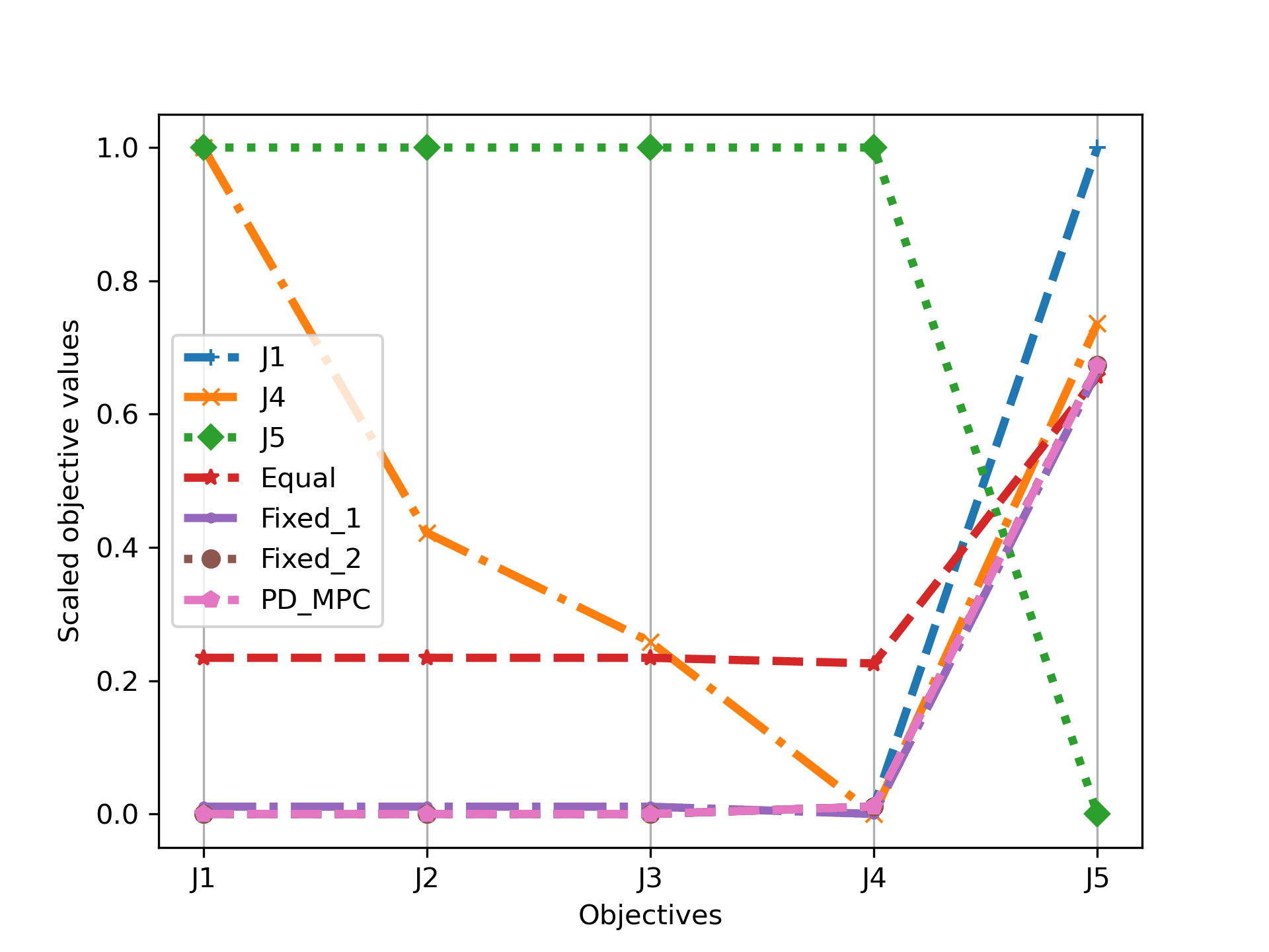
(b)

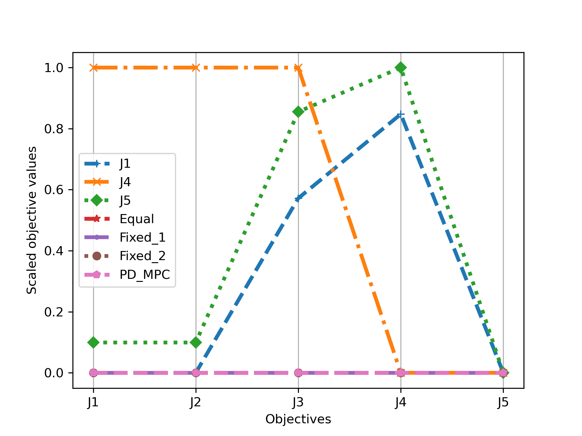
(c)

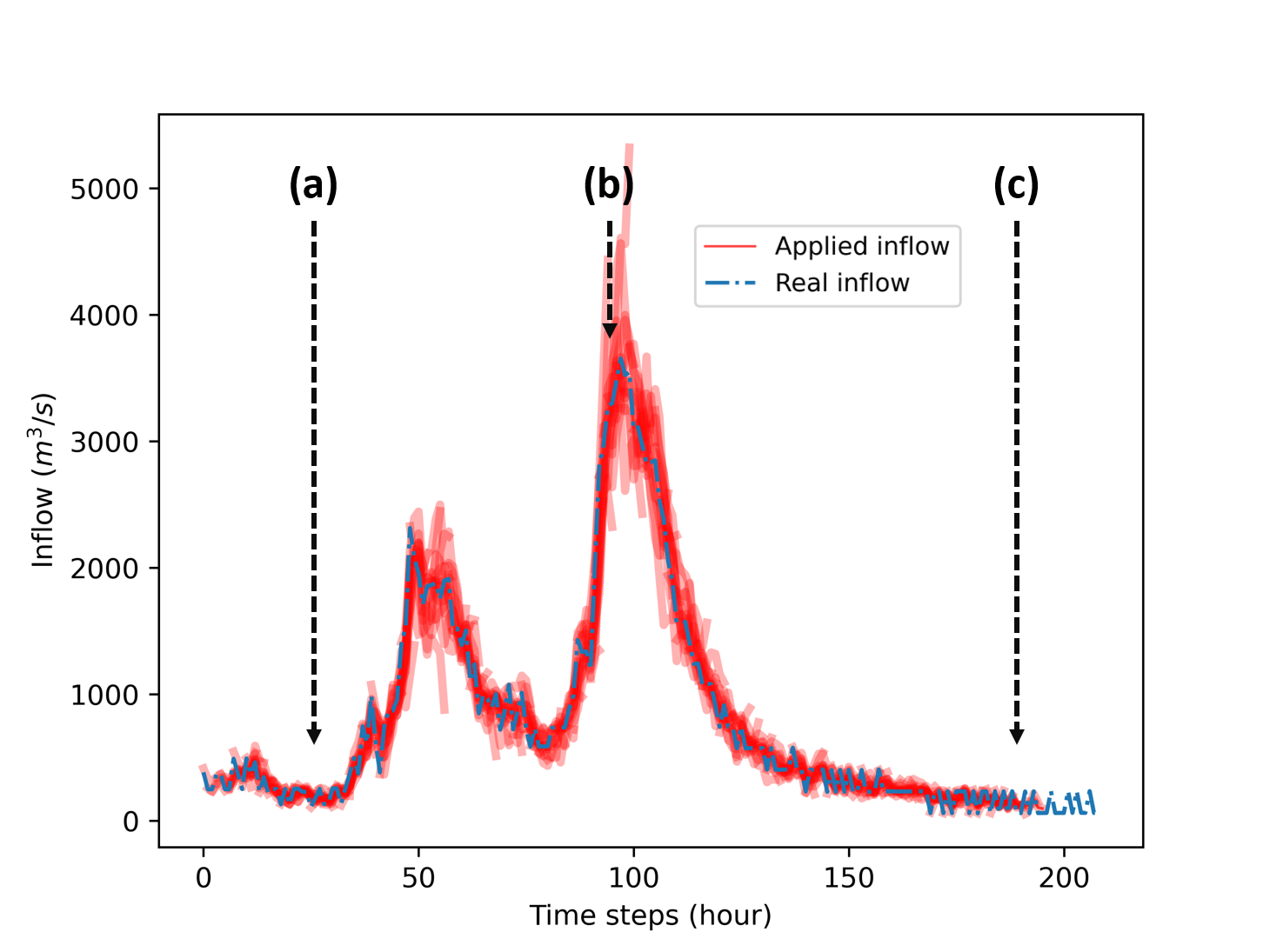
(d)

Figure 7: The parallel line plots for Event 1 with a 6-hour prediction horizon under uncertain inflow. (7(a)) At time step 25. (7(b)) At time step 97. (7(c)) At time step 160. (7(d)) The temporal location of each case in the event.

Figure 7 shows that the weight cases perform differently according to the hydrological state, and no single weight case is always dominant for all objectives. Objective values from PD-MPC consistently stay close to the lowest for all cases.

4.4 Discussion

It appears that the detailed design of practical objectives for reservoir flood control has not been thoroughly presented, and constructing a preference without a nonlinear formula is challenging. The receding optimal control of an MPC problem with numerous nonlinear objectives and constraints can become intractable to formulate and solve them online. Consequently, it seems that the operator’s preference has not been adequately incorporated, and static weights/parameters have been used for optimising reservoir flood control.

In this study, we harness the advantages of solving linear MPC problems by parameterising the nonlinear and dynamic preferences around the different operating points. This allows us to optimise weights/parameters set and control inputs simultaneously. Our approach is also in the spirit of multi-objective MPC methods for linear systems ([5]) where a time-varying, state-dependent decision criterion can be taken into account using parametric optimisation. First, we present objectives for practical flood control in detail. Some of them have not been extensively covered in prior literature despite their significant importance in practice, such as minimising the changes in outflow schedules. Subsequently, we categorize these objectives into linear and nonlinear ones following the parameterisation of the operator’s preference, i.e. the weights of objectives and parameters. We employ an Genetic Algorithm (GA)to optimise nonlinear objectives and constraints to derive the optimal weights/parameters of the linear MPC formulation at each time step. We refer to this framework as a Parameterised Dynamic Model Predictive Control (PD-MPC).

Through our numerical experiment with real flood inflows, we demonstrated that PD-MPC shows robustness to the inflow uncertainty. It is important to note that the PD-MPC framework does not directly handle inflow uncertainty. Instead, we rely on the robustness of the receding horizon MPC approach to address uncertainty and produce reliable results ([12]). Our results reveal that PD-MPC outperformed MPC formulations with fixed weights/parameters, even when these fixed weights/parameters were specifically designed for individual objectives. We showed that the weights/parameters in MPC formulations and the weights of objectives should also vary dynamically to adapt to changing conditions. PD-MPC then effectively adapted to the changing hydrological conditions and continuously updated the weights/parameters. This adaptability allowed it to make optimal decisions in real-time, resulting in better overall performance in terms of peak outflows, reservoir water levels, and the number of changes in outflow schedules. This adaptability is the key factor in its superior performance and is also essential for generating optimal control inputs reflecting the dynamic characteristic of the operator preferences.

Nevertheless, there are some limitations of this research. First, the MPC formulation applied here does not consider the final states of the system. MPC with policy search algorithms ([36]) or a value function produced by a Reinforcement Learning (RL) model ([3]) can give a chance to find the approximation of the terminal cost such that our MPC framework can consider the whole period of a flood event. To the best of our knowledge, this approach has never been applied to a reservoir system for the purpose of flood control. The second limitation is related to uncertainty. We showed that PD-MPC can generate acceptable control inputs under uncertainty from the inherent feedback mechanism of a receding horizon implementation; however, it is advisable to explore PD-MPC with stochastic/robust MPC ([35]) or Learning-based MPC ([17]) to ensure robustness by considering uncertainty explicitly. Finally, we did not consider the downstream impact of reservoir outflows for simplification. This should be considered important in practical operations. This can be included by using routing models or various heuristics suggested in many studies ([18, 30, 24]).

5 Conclusion

Optimal reservoir control is becoming increasingly important due to the environmental concerns associated with building new infrastructures and changing climate. This study addresses the limitations of existing reservoir control approaches from a practical point of view, highlighting the current limitations of the employed optimisation approaches to take into account specific operators’ preferences which may change in time. We assume dynamic preferences by operators in a multi-objective setting and show the dynamic characteristics of weights/parameters. We then propose a PD-MPC framework as a parameterised linear MPC with dynamic optimisation of weights/parameters via a model-based learning concept. We applied this methodology to the Daecheong reservoir and verified the dynamic-preference assumptions as well as tested the effectiveness of this framework. This study lays the foundation for developing more adaptive decision-making frameworks in reservoir flood control and other related fields, being closer to the actual set of preferences in reservoir management and hence having level of adoption by practitioners.

Despite some limitations, we think we can be one step closer to the practical implementation of optimisation approaches to real-time reservoir flood control through this work. This methodology cannot replace operators’ experience and manual operation completely, but we hope that operators can reduce flood risk as well as lessen their burden by receiving more convincing and applicable references.

Acknowledgement

We express our gratitude to K-water for their sponsorship of the first author and for sharing the data and information related to the Daecheong reservoir. The hydrological and operational data of the Daecheong reservoir is accessible to the public on K-water’s website (http://kwater.or.kr). We also thank SURF for allowing us to utilise the Dutch national e-infrastructure with the support of the SURF Cooperative using grant no. EINF-6342.

Data Availability

The data and code of this research are available at https://data.4tu.nl/private_datasets/ifVGAKGvBN-forAHCvaAnMjwfpvQljHxrq6Oki7u3UA. All data can be used under the CC-BY-4.0 licence. The hydrological and operational data of the Daecheong reservoir was obtained from K-water’s website (http://kwater.or.kr).

Appendix

Appendix A Evaluator

The evaluator estimates how much the control inputs from the MPC design with a particular weight/parameter set satisfy all objectives, including nonlinear objectives. The evaluator returns the (weighted) sum of penalties, and GA finds the weights/parameters which minimise the objective value, $E_{\mathbf{z},\mathbf{u}}$. Some weights/parameters in the evaluator, such as weights of each penalty value in Equation (16) to (22), need to be set by a discussion with operators. In this article, weights in Equation (15), which are from $w_{e,1}$ to $w_{e,7}$, are assigned to one, except for $w_{e,1}$, $w_{e,2}$, and $w_{e,3}$. The weights for $P_{\tilde{J1}}$ and $P_{\tilde{J2}}$ are set as 0.9 and 0.1, respectively. This is because both objectives work similarly, except for when the outflow changes abruptly. The weight for $P_{\tilde{J3}}$ is set as 0.2 because $P_{\tilde{J1}}$ works similarly to $P_{\tilde{J3}}$ in general. Therefore, although it is necessary to explicitly include $\tilde{J3}$ in MPC formulation with the same search range, assigning a small weight for this objective is reasonable in Evaluator. The return of the evaluator is as follows:

$$E_{z}=P_{\tilde{J1}}\times w_{e,1}+P_{\tilde{J2}}\times w_{e,2}+P_{\tilde{J3}}\times w_{e,2}+P_{\tilde{J4}}\times w_{e,3}+P_{\tilde{J5}}\times w_{e,4}+P_{\tilde{J6}}\times w_{e,5}+P_{\tilde{J7}}\times w_{e,6}+P_{\tilde{J8}}\times w_{e,7}.$$ (15)

Peak outflow: $\tilde{J1}$ and $\tilde{J2}$

To penalize for the largest outflow, an exponential function is introduced for the scaling:

$$\begin{split}P_{\tilde{J1}}&=A^{\frac{\max O_{spill,t}^{k}}{B}},\\ P_{\tilde{J2}}&=A^{\frac{\sum O_{spill,t}^{k}}{B\ timesH}},\end{split}$$ (16)

where the exponent, $A$, and the other constant, i.e. denominator $B$, are selected to prevent $P_{\tilde{J1}}$ and $P_{\tilde{J2}}$ from being too small or large. Here, we set $A$ to 2 and $B$ to 1000. The prediction horizon length is denoted as $H$. The results are not dependent hugely on these values.

Step-wise outflow changes in a prediction horizon: $\tilde{J3}$

Unlike the objective of Equation (1) in Section 2.1, the changes in outflows in a prediction horizon are considered binary numbers to penalize equally for any changes in outflows. This approach allows us to overcome a common challenge faced by linear MPC, i.e. the objective values fluctuate according to the state, and there are still tiny differences resulting in a penalty that is too minor to impact the optimization process significantly.

In addition, only increasing cases for the first four times are considered. First, a decrease in outflows is preferred, even though penalising only increases in outflows can lead to wild fluctuation when a prediction horizon is short. In reservoir flood control, a prediction horizon is generally short, as mentioned in Section 1. Therefore, only increases in outflows are considered by the evaluator because, in linear MPC formulation, both increases and decreases are penalised already. Furthermore, because a change in outflows for the distant future is not a big problem, even though no change is the best, the increases for the first four times, i.e. from $t$ = $k$ to $k+3$, are penalised.

$$\begin{split}P_{\tilde{J3}}&=\sum_{t=k}^{k+3}C_{3,t}\times\omega_{t},\\ &C_{3,t}=\begin{cases}1&\text{if }O_{spill,t+1}^{k}-O_{spill,t}^{k}>0,\\ 0&\text{otherwise,}\end{cases}\end{split}$$ (17)

where $C_{3,t}$ is also the binary value that is one when there is a change at time $t$ at time step $k$ from previous time steps $k-1$. The time-dependent weights $\omega_{t}$ decreases by time $t$ from 0.5 to 0.1.

Changes in outflows calculated at consecutive time steps: $\tilde{J4}$

A similar concept to the previous one is applied to changes in outflows calculated at consecutive time steps as follows:

$$\begin{split}P_{\tilde{J4}}&=\sum_{t=k+1}^{k+4}C_{4,t}\times\omega_{t},,\\ &C_{4,t}=\begin{cases}1&\text{if }O_{spill,t}^{k}-O_{spill,t}^{k-1}>0,\\ 0&\text{otherwise,}\end{cases}\end{split}$$ (18)

where $C_{4,t}$ is also the binary value that is one when there is a change at time $t$ at time step $k$ from previous time steps $k-1$. The weight $\omega_{t}$ is the same as the previous one in Equation (17).

Peak RWL: $\tilde{J5}$

A similar concept to Equation (3) in Section 2.1 is applied to the RWL, except for the $S_{H}$ because $S_{H}$ can change in PD-MPC. Instead, we add two different objectives, which are penalising when RWL increases in a prediction horizon and approaches FWL. The objective is as follows:

$$\begin{split}P_{\tilde{J5}}&=A^{\max(RWL_{t})-S_{U}}+A^{RWL_{k+H-1}-RWL_{k}}+A^{S_{L}-\min RWL_{t}}\times C+P_{FWL},\\ &P_{FWL}=\begin{cases}Largenumber&\text{if }\max RWL_{t}^{k}>FWL-0.1,\\ 0&\text{otherwise,}\end{cases}\end{split}$$ (19)

where the value in each parenthesis is zero if it is negative – we do not present a max function in Equation (19) so as not to look complicated. Because we want the penalties to have similar values, exponential functions are adopted. Here, we set $C$ as two same as $A$ to circumvent RWL falling under $S_{L}$. In addition, a large number, 2000 in our research, is added to $P_{\tilde{J5}}$ when RWL is close to FWL. The specific value of the large number is not crucial; it simply needs to be sufficiently large to prevent the selection of undesirable $\mathbf{z}$.

Continuity of spillway gates condition: $\tilde{J6}$

Because the evaluator and GA can optimise this nonlinear objective, we can remove it from the MPC design and formulate linear MPC. A similar formula as Equation (4) is adopted, but we express this also using an exponential function as follows:

$$\begin{split}P_{\tilde{J6}}&=\sum_{t=k}^{k+H-1}(A^{\rho_{t,close}}+A^{\rho_{t,open}})/C,\\ &\rho_{t,close}=\begin{cases}1&\text{if }O_{spill,t}^{k}>0\text{ and }O_{spill,t+1}^{k}=0,\\ 0&\text{otherwise.}\end{cases}\\ &\rho_{t,open}=\begin{cases}1&\text{if }O_{spill,t}^{k}=0\text{ and }O_{spill,t+1}^{k}>0,\\ 0&\text{otherwise.}\end{cases}\end{split}$$ (20)

where the exponent $A$ and denominator $C$ are selected to scale this objective value to one, so $A$ and $B$ are set as two.

Peak outflow compared to the peak inflow: $\tilde{J7}$

To penalize the largest outflow when it is above the peak inflow up to the current time step, we assign a large number of $\gamma$ to $\tilde{J7}$ when peak outflow is over peak inflow to the present, as mentioned in Section 2:

$$\begin{split}P_{\tilde{J7}}&=\begin{cases}Largenumber&\text{if }\max_{t}O_{total,t}^{k}>\max_{t}I_{t},\\ 0&\text{otherwise.}\end{cases}\end{split}$$ (21)

where $\gamma$ is set as 1000 in our research.

Turbine’s priority over spillway: $\tilde{J8}$

Outflows by turbines should precede opening spillway gates. In some cases, such as in South Korea, changing turbine outflows is not considered flood control because the total capacity of all turbines is generally much smaller than the spillway capacity. Therefore, if the optimal turbine outflows are less than the total capacity of turbines, even if the optimal spillway outflow is larger than zero, i.e. spillway gates open, the evaluator will penalize the weight/parameter set to prevent GA from selecting the set. This is formulated as below:

$$P_{\tilde{J8}}=\begin{cases}\text{Large number}&\text{if }O_{spill,t}^{k}>0\text{ and }O_{turb,t}^{k}<MO_{turb},\\ 0&\text{otherwise,}\end{cases}$$ (22)

where $O_{turb,t}^{k}$ is outflow via turbines at time $t$ decided at time step $k$, and $MO_{turb}$ is the outflow capacity of turbines. The large number, here, is set to 100000 to rigorously prevent this scenario.

Appendix B Flood events used for experiments and uncertain inflow generated to test performance

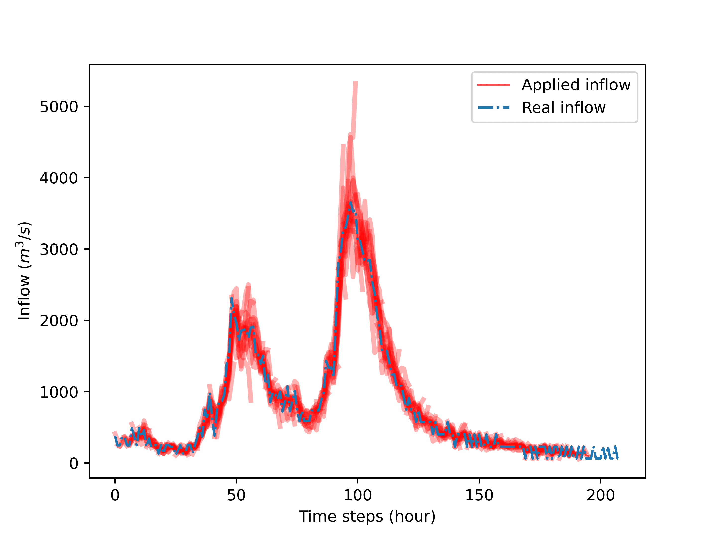
(a)

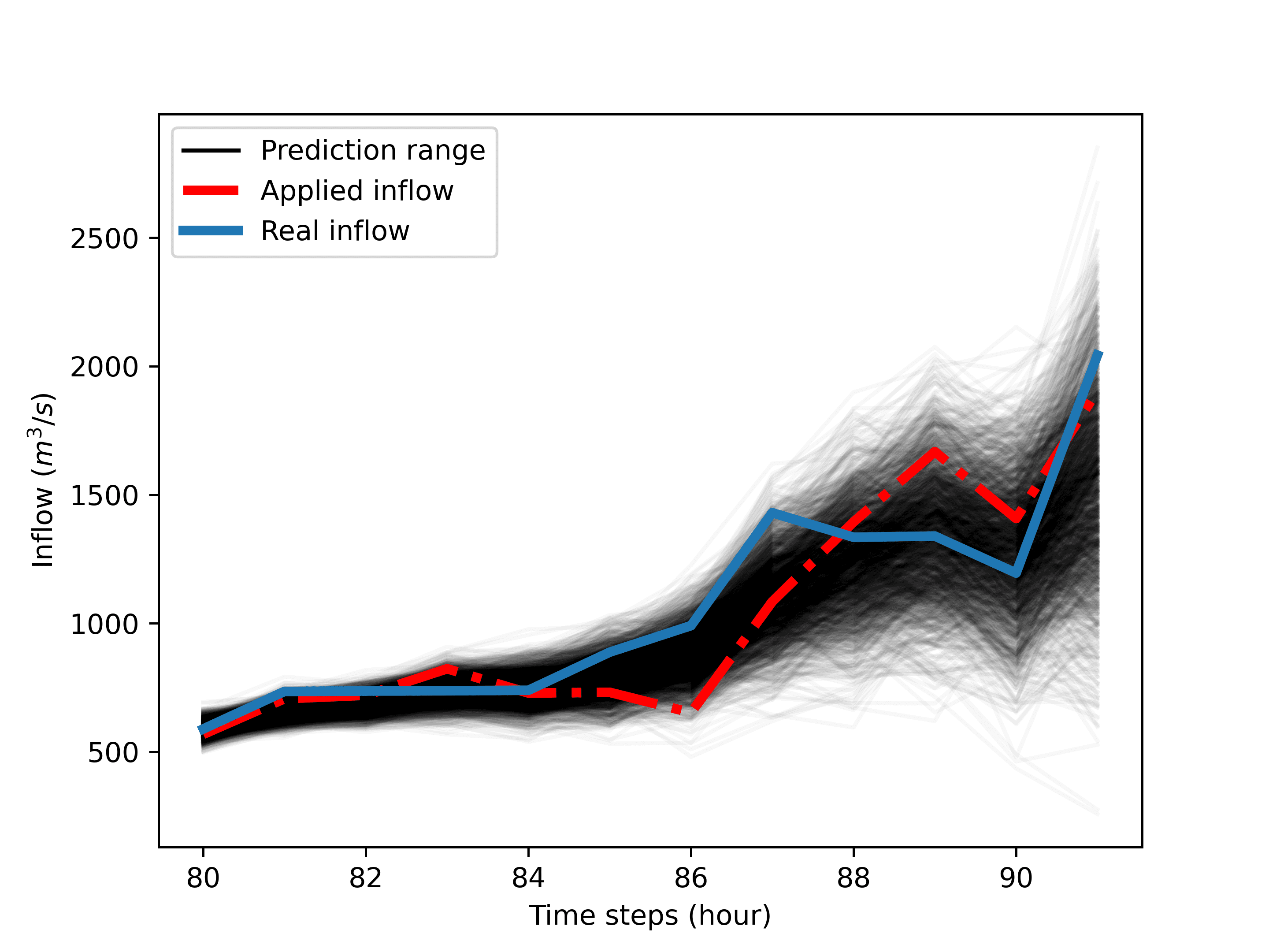
(b)

Figure 8: Example of real and predicted inflow hydrographs for Event 1 when a prediction horizon is 12 hours. (8(a)) The hydrograph for the whole event period (8(b)) An example of predicted inflow at time step $80$.

We present three flood events, as depicted in Figure 8 and 9. In these illustrations, the ‘applied inflow’ is highlighted in red, representing the overlay of uncertain inflows generated individually for each time step within a prediction horizon. For instance, in Figure 8(a), one red line representing an uncertain inflow starting from time step 0 to 11 is presented, and another uncertain inflow starting from time step 1 to 12 is presented. This pattern continues for each subsequent time step until the last time step. There are a total of 184 different uncertain inflows, all within a 12-hour prediction horizon, depicted in this figure. In Figure 8(b), a total of 2000 black lines illustrate uncertain inflows by incorporating random errors into the actual inflow data.

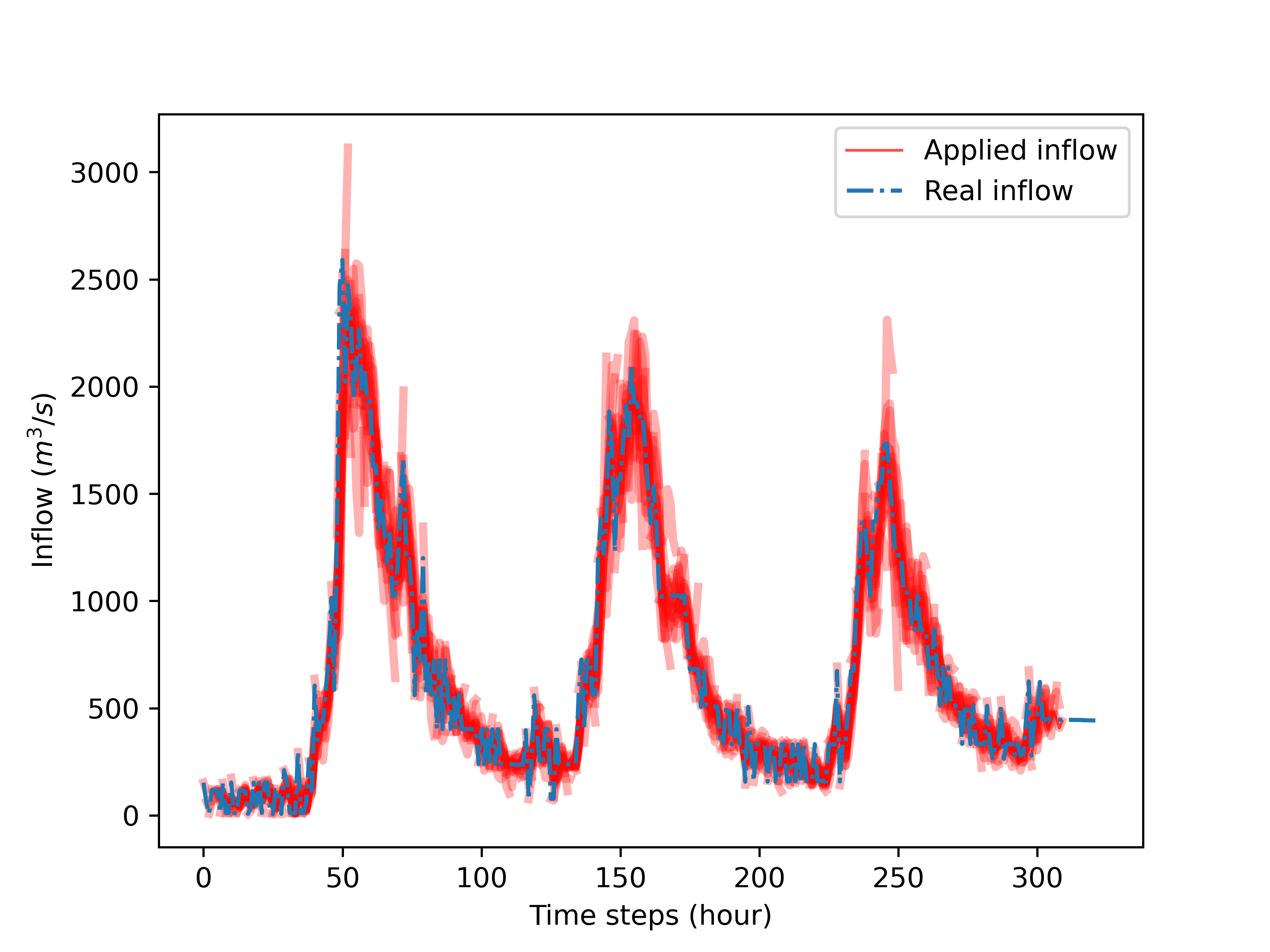
(a)

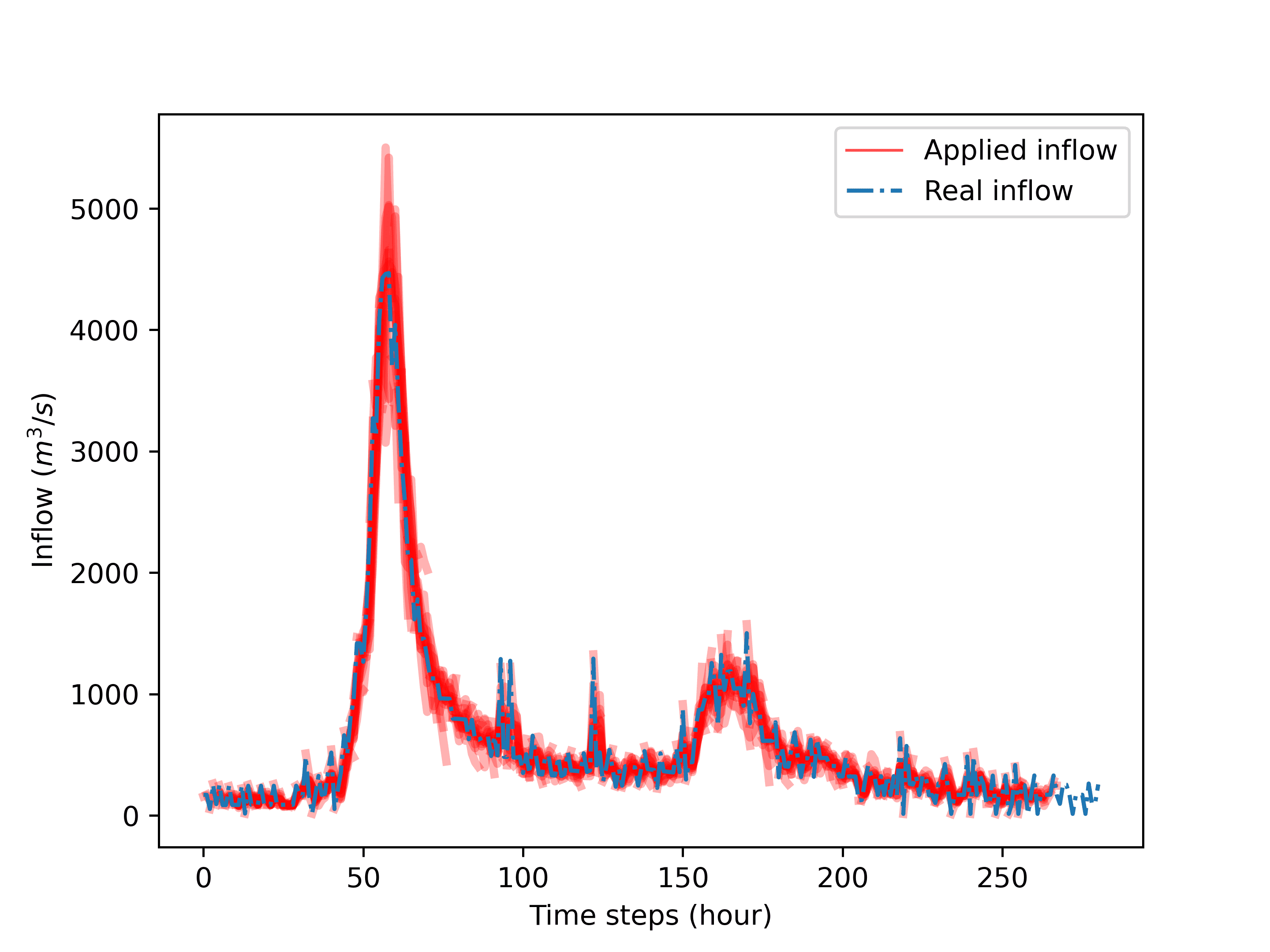
(b)

Figure 9: Example of real and predicted inflow hydrographs with a 12-hour prediction horizon. (9(a)) For Event 2. (9(b)) For Event 3.

Appendix C Detailed results of the PD-MPC framework

C.1 Detailed result of PD-MPC

Figure 10 illustrates the optimal outflows with uncertain inflow and RWL for Event 1 across different prediction horizons. The generated optimal outflows, denoted as $\mathbf{u}^{k}$s, are represented by dashed lines of various colours, overlaid with the red line indicating the total outflows in the figures. For instance, in Figure 10(d), where outflows are decreasing, a 24-hour prediction horizon leads to numerous changes in outflows. It is worth noting that while all changes are penalized in MPC, the evaluator does not penalize changes beyond four hours for each prediction horizon, as explained in Section 3.2.3 and Appendix A.

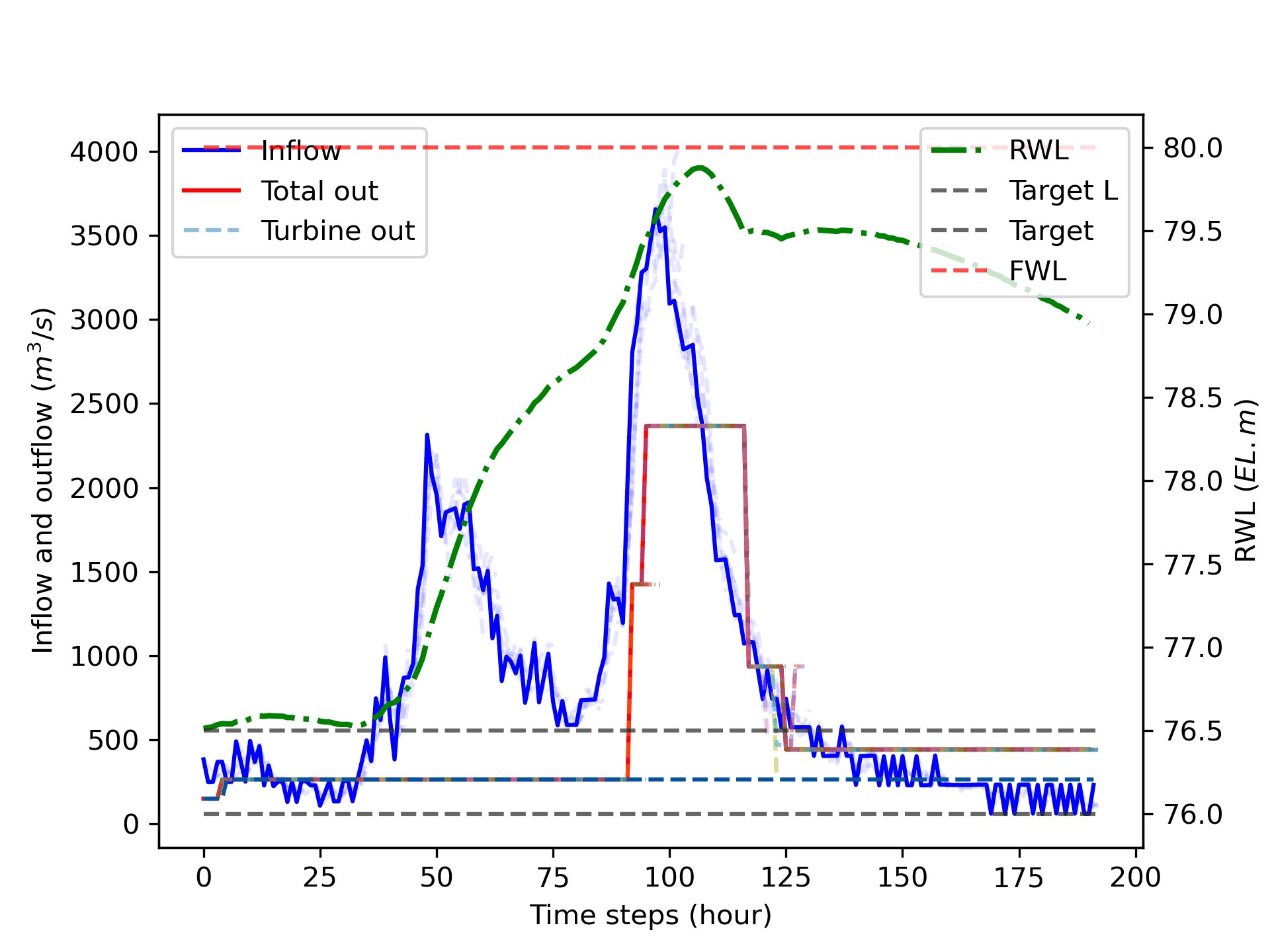
(a)

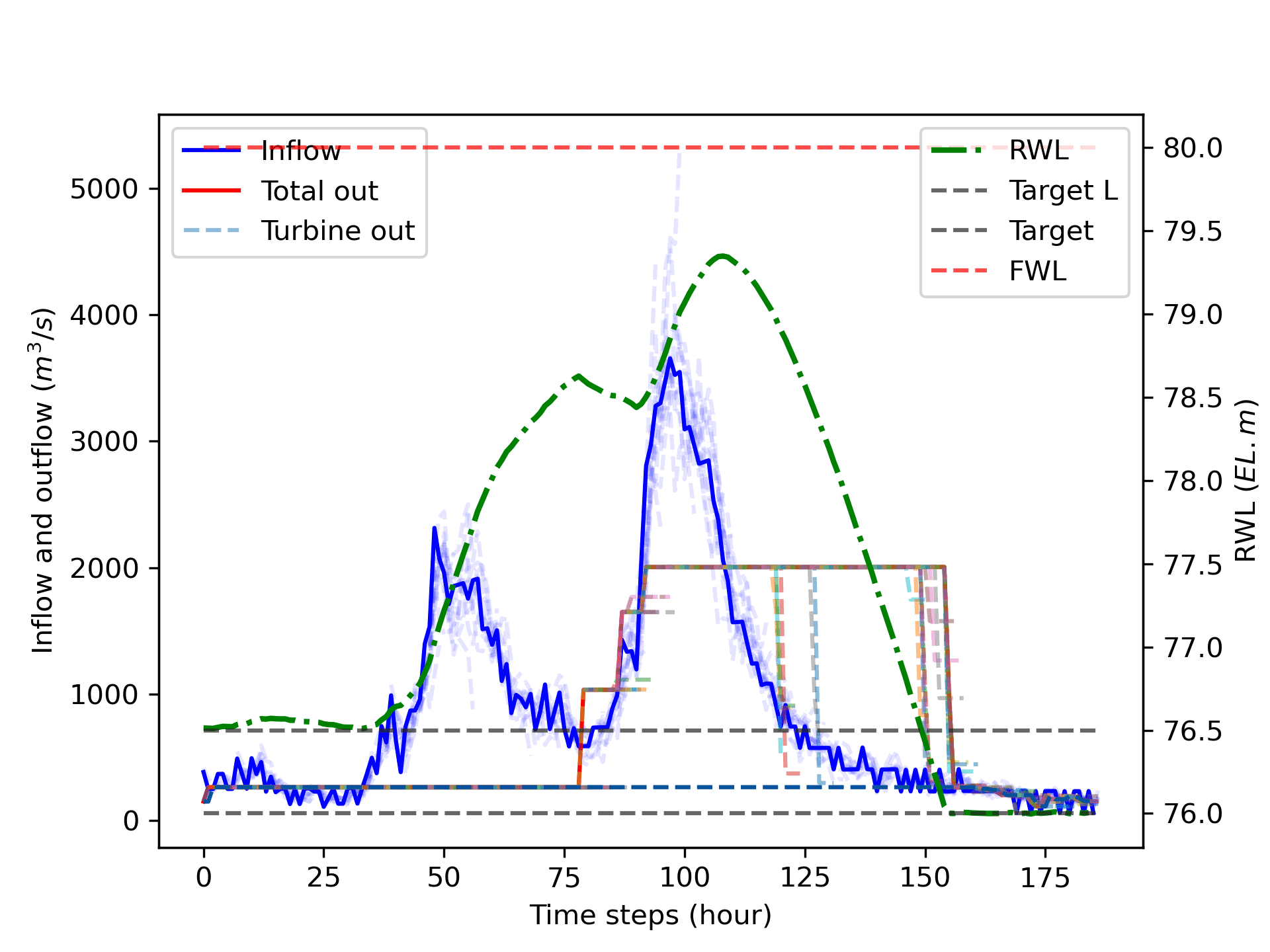
(b)

(c)

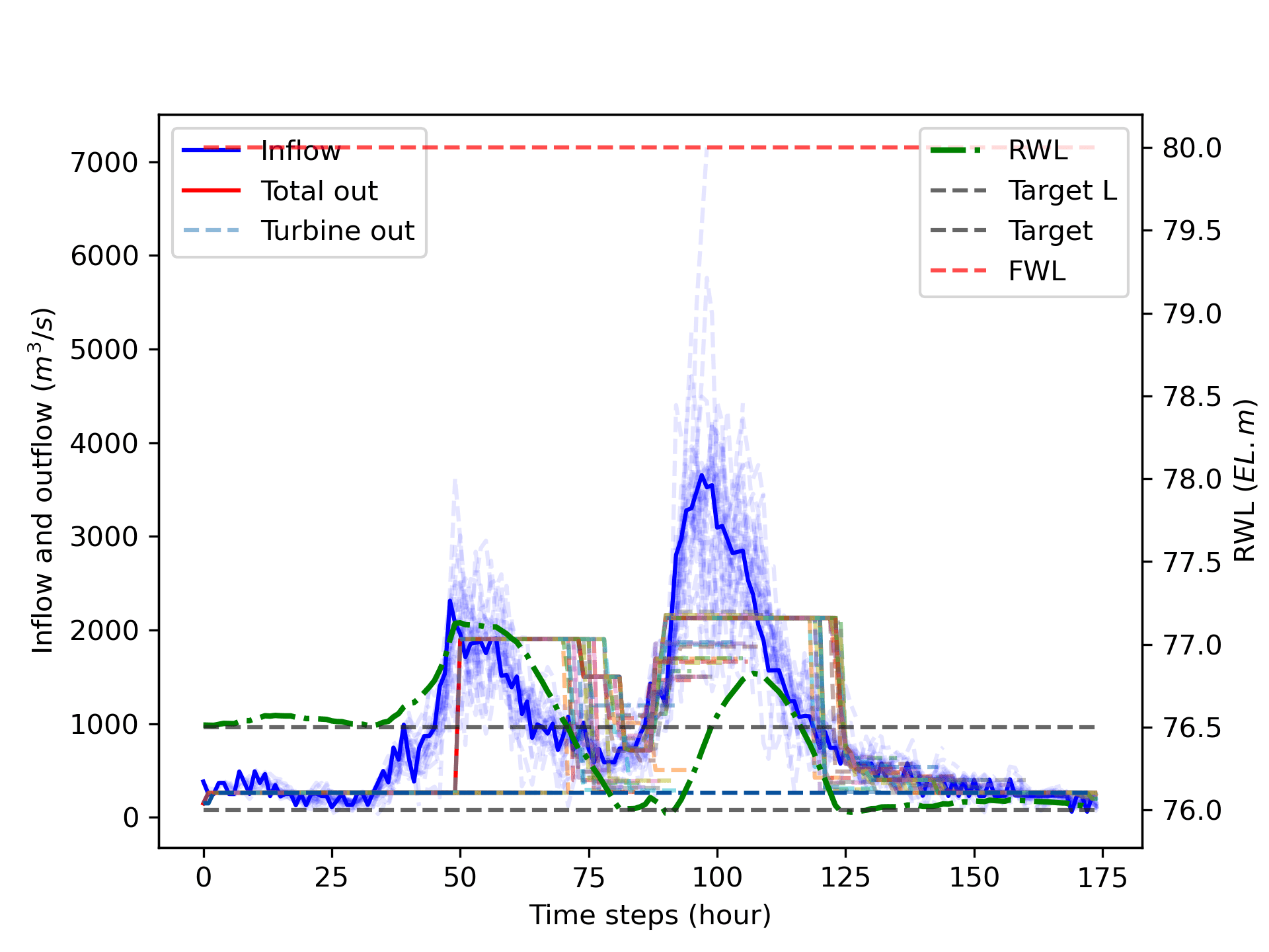
(d)

Figure 10: Hydrographs under uncertain inflow and different prediction horizons for Event 1. (10(a)) 6 hours. (10(b)) 12 hours. (10(c)) 18 hours. (10(d)) 24 hours.

The detailed result of the numerical experiment is presented in Table 4 for uncertain inflow and Table 5 for certain inflow.

Table 4: The detailed result of PD-MPC under uncertain inflow.

Prediction horizon	Event	Peak outflow ($m^{3}/s$)	Peak RWL (EL. m)	Lowest RWL (EL. m)	Changes between time steps
6	1	2,367	79.88	76.50	9
12	1	2,005	79.35	76.00	9
18	1	2,296	78.67	76.00	11
24	1	2,128	77.13	75.98	9
6	2	1,919	79.82	76.13	20
12	2	1,591	79.04	76.00	8
18	2	1,273	77.56	76.00	21
24	2	1,915	76.81	76.01	30
6	3	2,105	79.81	76.34	13
12	3	1,323	78.37	75.99	10
18	3	1,245	78.19	76.00	18
24	3	1,273	78.07	76.01	38

Table 5: The detailed result of PD-MPC under certain inflow.

Prediction horizon	Event	Peak outflow ($m^{3}/s$)	Peak RWL (EL. m)	Lowest RWL (EL. m)	Changes between time steps
6	1	2,332	79.89	76.50	9
12	1	2,153	79.27	76.00	4
18	1	2,290	78.60	76.00	11
24	1	1,873	77.13	75.93	4
6	2	2,051	79.84	76.19	9
12	2	1,499	79.09	75.99	8
18	2	990	77.38	76.00	11
24	2	1,870	76.92	76.00	17
6	3	2,078	79.82	76.32	8
12	3	1,051	78.59	76.00	11
18	3	1,104	78.33	75.95	9
24	3	1,374	77.91	76.00	18

Under uncertain inflow conditions for Event 1, a comparison of the results between PD-MPC and the Fixed cases is presented in Table 6. PD-MPC outperforms the Fixed cases for all items in the table.

Table 6: The comparison between PD-MPC and the Fixed cases for Event 1 under uncertain inflow.

	Prediction horizon	Peak outflow ($m^{3}/s$)	Peak RWL (EL. m)	Lowest RWL (EL. m)	Changes between time steps
PD-MPC	6	2,367	79.88	76.50	9
Fixed 1	6	3,710	79.10	75.97	13
Fixed 2	6	3,617	79.31	76.31	28
PD-MPC	12	2,005	79.35	76.00	9
Fixed 1	12	3,267	79.19	76.37	10
Fixed 2	12	2,759	79.35	76.34	37
PD-MPC	18	2,259	78.67	76.00	11
Fixed 1	18	2,578	79.35	76.34	12
Fixed 2	18	2,551	79.60	76.31	48
PD-MPC	24	2,128	77.13	75.98	9
Fixed 1	24	2,259	78.03	75.95	16
Fixed 2	24	2,223	79.32	76.28	33

Figure 11, 12, and 13 show the effect of the evaluator by changing the weight of the objective, which minimises the changes in outflow schedules, i.e. $\tilde{J4}$ in Section 2.1, in the evaluator.

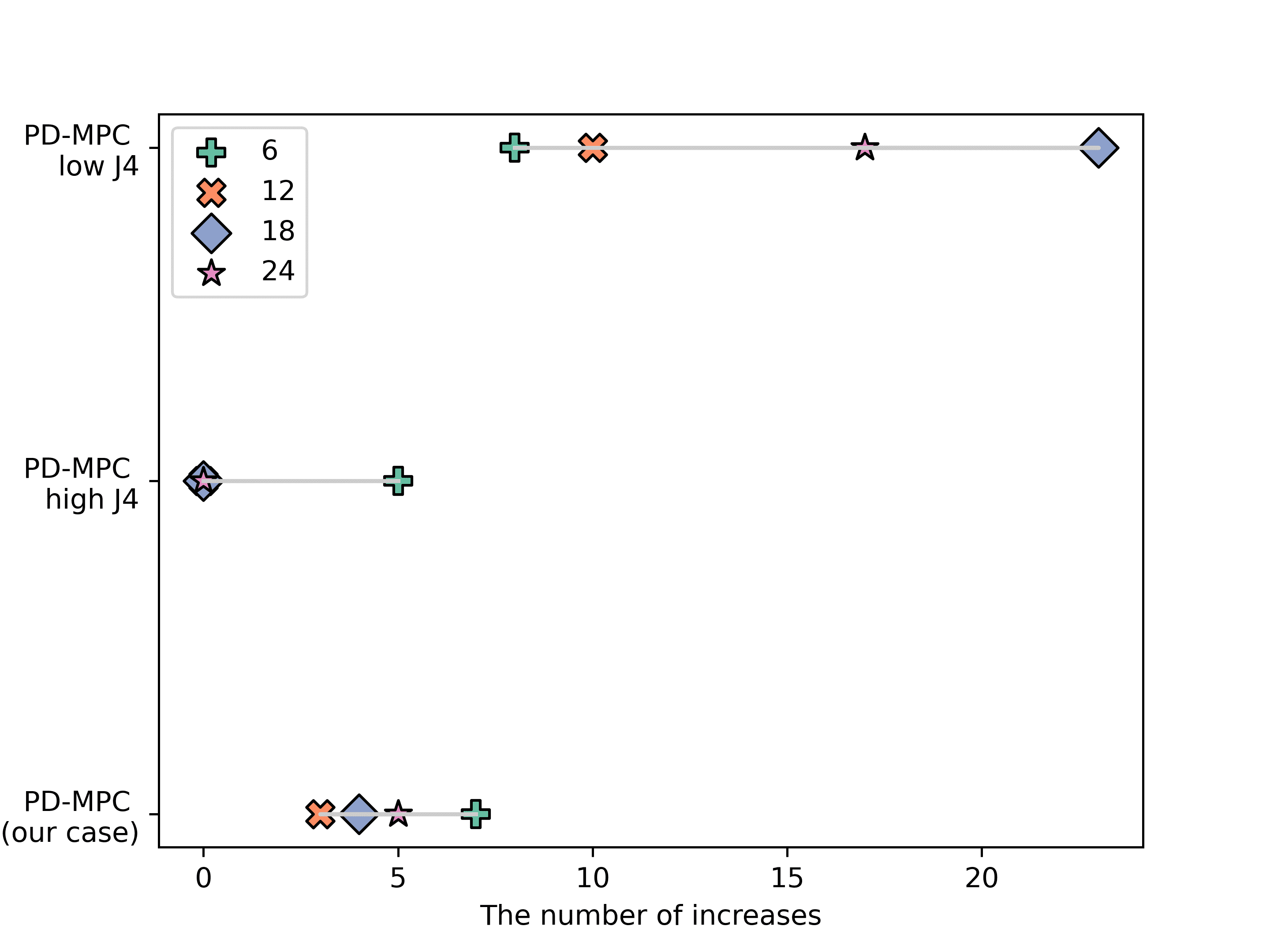
(a)

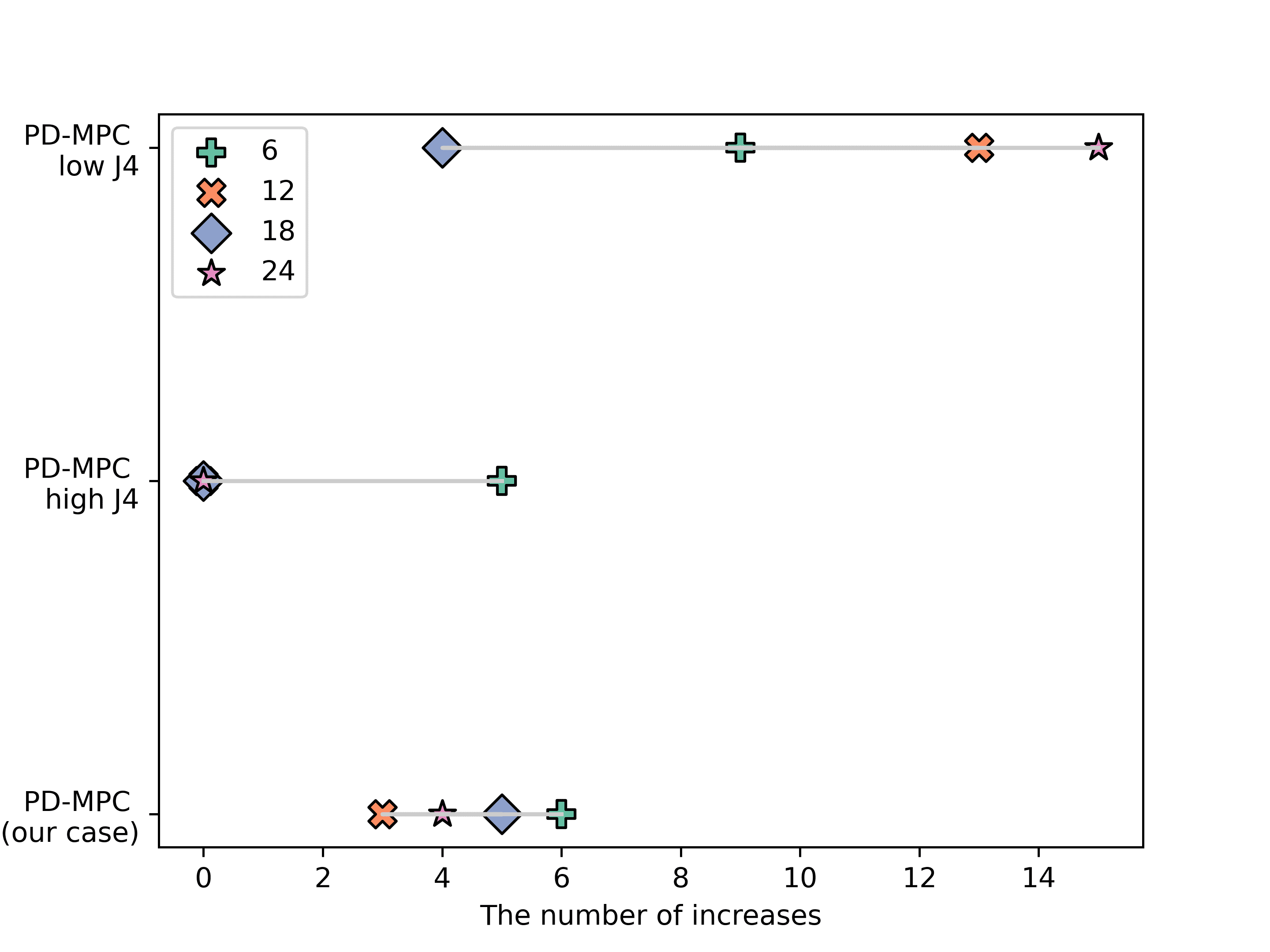
(b)

Figure 11: The number of increases with different evaluator settings for Event 1. (11(a)) under uncertain inflow. (11(b)) under certain inflow.

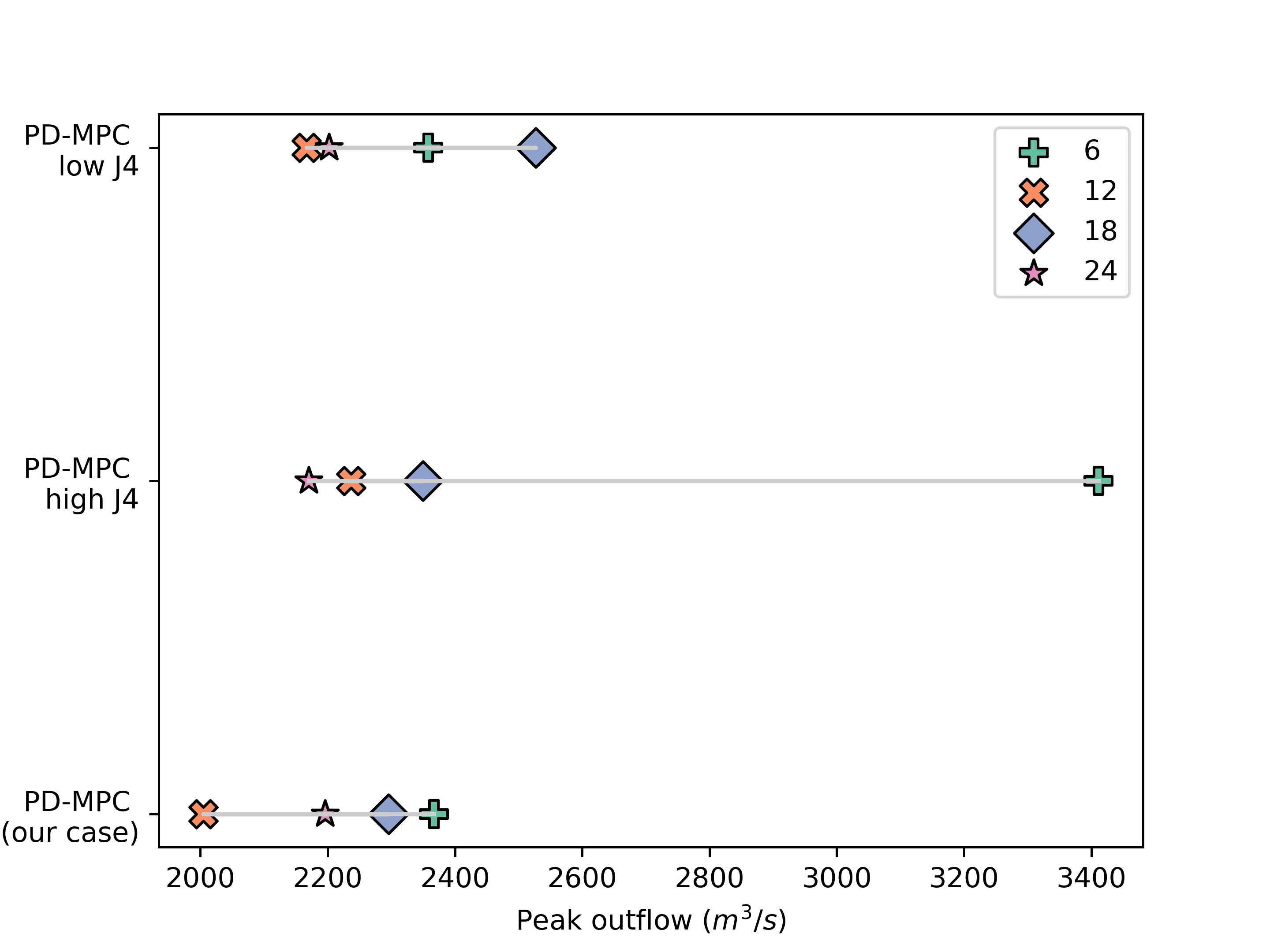
(a)

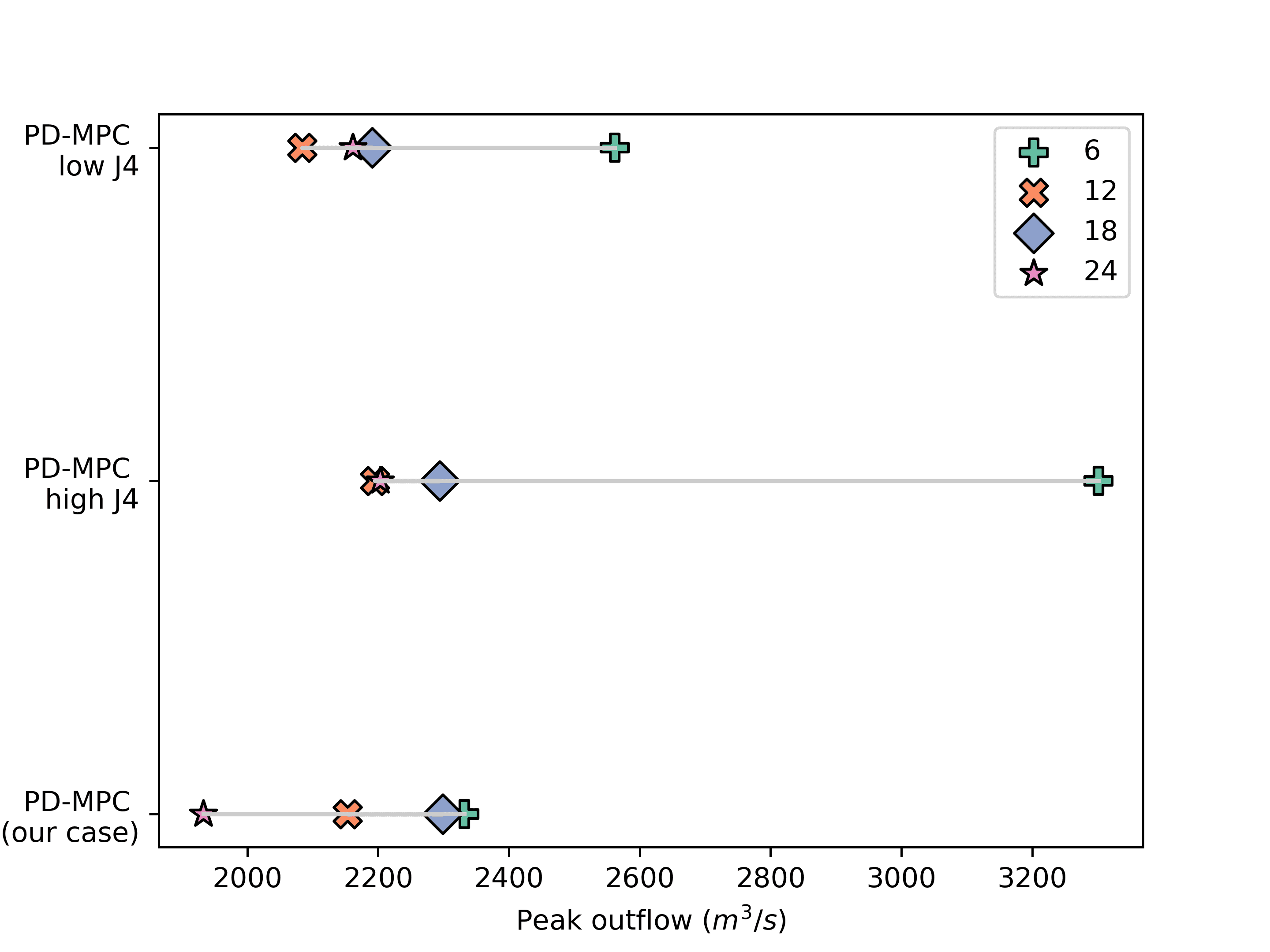
(b)

Figure 12: The peak outflow with different evaluator settings for Event 1. (12(a)) under uncertain inflow. (12(b)) under certain inflow.

(a)

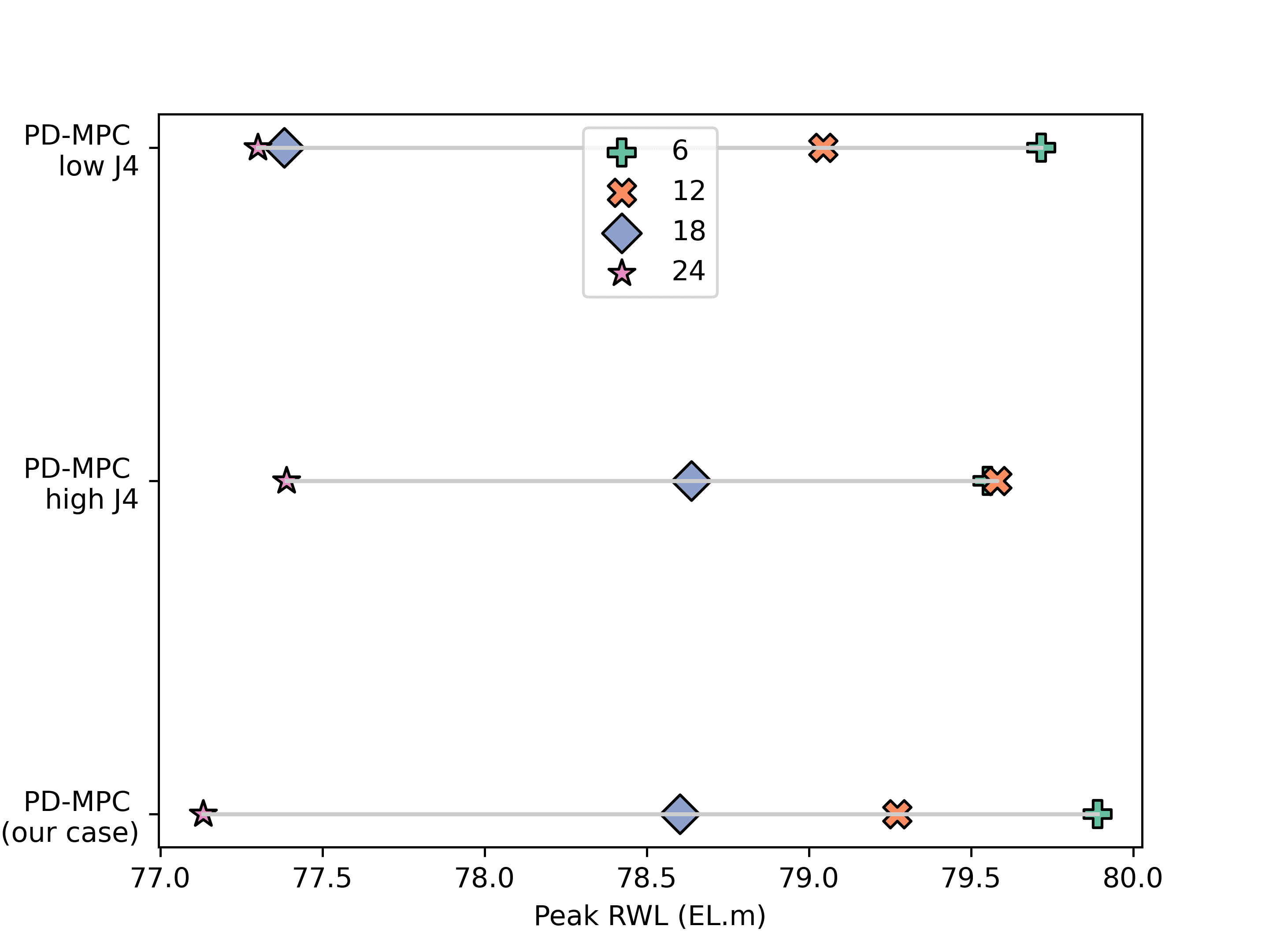
(b)

Figure 13: The peak RWL with different evaluator settings for Event 1. (13(a)) under uncertain inflow. (13(b)) under certain inflow.

References

- [1] A. Ahmad, A. El-Shafie, S… Razali and Z.. Mohamad “Reservoir Optimization in Water Resources: a Review” In Water Resources Management 28.11, 2014, pp. 3391–3405
- [2] Mihai Anitescu “On solving mathematical programs with complementarity constraints as nonlinear programs” In Preprint ANL/MCS-P864-1200, Argonne National Laboratory, Argonne, IL 3, 2000
- [3] Javier Arroyo, Carlo Manna, Fred Spiessens and Lieve Helsen “Reinforced model predictive control (RL-MPC) for building energy management” In Applied Energy 309, 2022, pp. 118346
- [4] B.. Aydin et al. “Nonlinear model predictive control of salinity and water level in polder networks: Case study of Lissertocht catchment” In Agricultural Water Management 264, 2022
- [5] Alberto Bemporad and David Muñoz Peña “Multiobjective model predictive control” In Automatica 45.12 Elsevier, 2009, pp. 2823–2830
- [6] M. Breckpot, O.. Agudelo and B. De Moor “Flood Control with Model Predictive Control for River Systems with Water Reservoirs” In Journal of Irrigation and Drainage Engineering 139.7, 2013, pp. 532–541
- [7] Carlos Ignacio Hernández Castellanos, Sina Ober-Blöbaum and Sebastian Peitz “Explicit Multi-objective Model Predictive Control for Nonlinear Systems Under Uncertainty” In arXiv preprint arXiv:2002.06006, 2020
- [8] Andrea Castelletti et al. “Model Predictive Control of water resources systems: A review and research agenda” In Annual Reviews in Control Elsevier, 2023
- [9] L.. Chang “Guiding rational reservoir flood operation using penalty-type genetic algorithm” In Journal of Hydrology 354.1-4, 2008, pp. 65–74
- [10] C. Chen, Y.. Yuan and X.. Yuan “An Improved NSGA-III Algorithm for Reservoir Flood Control Operation” In Water Resources Management 31.14, 2017, pp. 4469–4483
- [11] Juan Chen et al. “A multi-objective risk management model for real-time flood control optimal operation of a parallel reservoir system” In Journal of Hydrology 590, 2020, pp. 125264
- [12] Giuseppe De Nicolao, Lalo Magni and Riccardo Scattolini “On the robustness of receding-horizon control with terminal constraints” In IEEE Transactions on Automatic Control 41.3 IEEE, 1996, pp. 451–453
- [13] D.. Delgoda, S.. Saleem, M.. Halgamuge and H. Malano “Multiple Model Predictive Flood Control in Regulated River Systems with Uncertain Inflows” In Water Resources Management 27.3, 2013, pp. 765–790
- [14] Ahmed Fawzy Gad “Pygad: An intuitive genetic algorithm python library” In arXiv preprint arXiv:2106.06158, 2021
- [15] M. Giuliani, J.. Lamontagne, P.. Reed and A. Castelletti “A State-of-the-Art Review of Optimal Reservoir Control for Managing Conflicting Demands in a Changing World” In Water Resources Research 57.12, 2021
- [16] William E Hart, Jean-Paul Watson and David L Woodruff “Pyomo: modeling and solving mathematical programs in Python” In Mathematical Programming Computation 3, 2011, pp. 219–260
- [17] Lukas Hewing, Kim P Wabersich, Marcel Menner and Melanie N Zeilinger “Learning-based model predictive control: Toward safe learning in control” In Annual Review of Control, Robotics, and Autonomous Systems 3, 2020, pp. 269–296
- [18] N.. Hsu and C.. Wei “A multipurpose reservoir real-time operation model for flood control during typhoon invasion” In Journal of Hydrology 336.3-4, 2007, pp. 282–293
- [19] Sharad K Jain, LS Shilpa, Deepti Rani and KP Sudheer “State-of-the-art review: operation of multi-purpose reservoirs during flood season” In Journal of Hydrology, 2023, pp. 129165
- [20] S. Katoch, S.. Chauhan and V. Kumar “A review on genetic algorithm: past, present, and future” In Multimedia Tools and Applications 80.5, 2021, pp. 8091–8126
- [21] Abhishek Kumar et al. “A review of multi criteria decision making (MCDM) towards sustainable renewable energy development” In Renewable and Sustainable Energy Reviews 69, 2017, pp. 596–609
- [22] Michal Kvasnica “Implicit vs explicit MPC—Similarities, differences, and a path owards a unified method” In 2016 European Control Conference (ECC), 2016, pp. 603–603 IEEE
- [23] J.. Labadie “Optimal operation of multireservoir systems: State-of-the-art review” In Journal of Water Resources Planning and Management 130.2, 2004, pp. 93–111
- [24] L. Le Ngo, H. Madsen and D. Rosbjerg “Simulation and optimisation modelling approach for operation of the Hoa Binh reservoir, Vietnam” In Journal of Hydrology 336.3-4, 2007, pp. 269–281
- [25] J.. Luo, C. Chen and J.. Xie “Multi-objective Immune Algorithm with Preference-Based Selection for Reservoir Flood Control Operation” In Water Resources Management 29.5, 2015, pp. 1447–1466
- [26] X.. Ma et al. “MOEA/D with biased weight adjustment inspired by user preference and its application on multi-objective reservoir flood control problem” In Soft Computing 20.12, 2016, pp. 4999–5023
- [27] Andrew Makhorin “Glpk (gnu linear programming kit), version 5.0” URL: http://www.gnu.org/software/glpk/
- [28] Nay Myo Lin et al. “Multi-objective model predictive control for real-time operation of a multi-reservoir system” In Water 12.7 MDPI, 2020, pp. 1898
- [29] Sina Ober-Blöbaum and Sebastian Peitz “Explicit multiobjective model predictive control for nonlinear systems with symmetries” In International Journal of Robust and Nonlinear Control 31.2 Wiley Online Library, 2021, pp. 380–403
- [30] Y. Peng, K. Chen, H.. Yan and X.. Yu “Improving Flood-Risk Analysis for Confluence Flooding Control Downstream Using Copula Monte Carlo Method” In Journal of Hydrologic Engineering 22.8, 2017
- [31] F. Pianosi, B. Dobson and T. Wagener “Use of Reservoir Operation Optimization Methods in Practice: Insights from a Survey of Water Resource Managers” In Journal of Water Resources Planning and Management 146.12, 2020
- [32] K.. Powell, A.. Eaton, J.. Hedengren and T.. Edgar “A Continuous Formulation for Logical Decisions in Differential Algebraic Systems using Mathematical Programs with Complementarity Constraints” In Processes 4.1, 2016
- [33] Y.. Qi et al. “Reservoir flood control operation using multi-objective evolutionary algorithm with decomposition and preferences” In Applied Soft Computing 50, 2017, pp. 21–33
- [34] Gilberto Reynoso-Meza, Victor Henrique Alves Ribeiro and Elizabeth Pauline Carreño-Alvarado “A comparison of preference handling techniques in multi-objective optimisation for water distribution systems” In Water 9.12 MDPI, 2017, pp. 996
- [35] M. Saltık et al. “An outlook on robust model predictive control algorithms: Reflections on performance and computational aspects” In Journal of Process Control 61, 2018, pp. 77–102
- [36] Y.. Song and D. Scaramuzza “Policy Search for Model Predictive Control With Application to Agile Drone Flight” In Ieee Transactions on Robotics 38.4, 2022, pp. 2114–2130
- [37] Rong Tang et al. “Reference point based multi-objective optimization of reservoir operation: a comparison of three algorithms” In Water resources management 34 Springer, 2020, pp. 1005–1020
- [38] G. Uysal, R. Alvarado-Montero, D. Schwanenberg and A. Sensoy “Real-Time Flood Control by Tree-Based Model Predictive Control Including Forecast Uncertainty: A Case Study Reservoir in Turkey” In Water 10.3, 2018
- [39] Peter-Jules Van Overloop “Model predictive control on open water systems” IOS Press, 2006
- [40] Handing Wang, Markus Olhofer and Yaochu Jin “A mini-review on preference modeling and articulation in multi-objective optimization: current status and challenges” In Complex & Intelligent Systems 3 Springer, 2017, pp. 233–245
- [41] M. Xu, P.. Overloop and N.. Giesen “On the study of control effectiveness and computational efficiency of reduced Saint-Venant model in model predictive control of open channel flow” In Advances in Water Resources 34.2, 2011, pp. 282–290
- [42] Xinting Yu, Yue-Ping Xu, Haiting Gu and Yuxue Guo “Multi-objective robust optimization of reservoir operation for real-time flood control under forecasting uncertainty” In Journal of Hydrology 620, 2023, pp. 129421
- [43] Stanley Zionts “MCDM—If not a roman numeral, then what?” In Interfaces 9.4 INFORMS, 1979, pp. 94–101