Better by Default: Strong Pre-Tuned MLPs and Boosted Trees on Tabular Data

Abstract

For classification and regression on tabular data, the dominance of gradient-boosted decision trees (GBDTs) has recently been challenged by often much slower deep learning methods with extensive hyperparameter tuning. We address this discrepancy by introducing (a) RealMLP, an improved multilayer perceptron (MLP), and (b) improved default parameters for GBDTs and RealMLP. We tune RealMLP and the default parameters on a meta-train benchmark with 71 classification and 47 regression datasets and compare them to hyperparameter-optimized versions on a disjoint meta-test benchmark with 48 classification and 42 regression datasets, as well as the GBDT-friendly benchmark by Grinsztajn et al. (2022). Our benchmark results show that RealMLP offers a better time-accuracy tradeoff than other neural nets and is competitive with GBDTs. Moreover, a combination of RealMLP and GBDTs with improved default parameters can achieve excellent results on medium-sized tabular datasets (1K–500K samples) without hyperparameter tuning.

1 Introduction

Perhaps the most common type of data in practical machine learning (ML) is tabular data, characterized by a fixed number of numerical or categorical features (columns), lacking the spatiotemporal structure of most other data types such as image or text data. The moderate dimensionality and lack of symmetries make tabular data accessible to a wide variety of machine learning methods. While tabular data is very diverse and no method is dominant on all datasets, gradient-boosted decision trees (GBDTs) have demonstrated excellent results on benchmarks [57, 19, 43], although their superiority has been challenged by a variety of deep learning methods [3].

GBDTs and neural networks (NNs) are often compared using extensive hyperparameter optimization. This can be especially expensive for NNs, as multilayer perceptrons (MLPs) and Transformer-based models are roughly one and two orders of magnitude slower than typical GBDTs, respectively [19, 43]. To address this issue, we investigate the potential of improved MLPs and better dataset-independent default parameters for MLPs and GBDTs. Specifically, we compare the library defaults (D) to our tuned defaults (TD) and (dataset-dependent) hyperparameter optimization (HPO).

Besides offering convenient baselines for quick exploration and benchmarking, good default parameters also play an important role in automated ML (AutoML). AutoGluon [11] demonstrated that stacking and ensembling models with fixed parameters outperforms other AutoML approaches based on hyperparameter optimization [14]. Without stacking and ensembling, McElfresh et al. [43] have argued that light hyperparameter tuning for GBDTs is often more effective than trying out NNs. Here, we argue that even without stacking and ensembling, when using well-chosen default parameters for GBDTs and our improved MLPs, trying GBDTs and MLPs is often faster and more beneficial than (naively) optimizing the hyperparameters of a single method.

1.1 Contribution

The problem of finding better default parameters can be seen as a meta-learning problem [63]. We employ a meta-train benchmark consisting of 118 datasets on which the default hyperparameters are optimized, and a disjoint meta-test benchmark consisting of 90 datasets on which they are evaluated. We consider separate default parameters for classification, optimized for classification error, and for regression, optimized for RMSE. Our benchmarks do not contain missing numerical values, and we restrict ourselves to sizes between 1K and 500K samples, cf. Section 2.

In Section 3, we introduce RealMLP, which improves on standard MLPs through a bag of tricks and better default parameters, tuned entirely on the meta-train benchmark. We introduce many novel or nonstandard components, such as preprocessing using robust scaling and smooth clipping, a new numerical embedding variant, a diagonal weight layer, new schedules, different initialization methods, etc. Our benchmark results demonstrate that it outperforms other comparably fast NNs from the literature and can be competitive with GBDTs. We make RealMLP and the other models available through a scikit-learn interface.

In Section 4, we provide new default parameters, tuned on the meta-train benchmark, for XGBoost [10], LightGBM [31], and CatBoost [51]. While they cannot match HPO on average, they outperform the library defaults on the meta-test benchmark.

In Section 5, we evaluate these and other models on the meta-test benchmark and the benchmark by Grinsztajn et al. [19]. We also investigate several possibilities for algorithm selection and ensembling, demonstrating that algorithm selection over default methods provides a better time-performance tradeoff than HPO, thanks to our new improved default parameters and MLP.

Our code (including scikit-learn interfaces) for meta-train and meta-test benchmarks is available at +rCl+x* github.com/dholzmueller/pytabkit At https://github.com/LeoGrin/tabular-benchmark/tree/better_by_default, we provide code for the adapted Grinsztajn et al. [19] benchmark. Our code and benchmark data will be archived at https://doi.org/10.18419/darus-4255.

1.2 Related Work

Neural networks

[3] review deep learning on tabular data and identify three main classes of methods: Data transformation methods, specialized architectures, and regularization models. In particular, recent research has mainly focused on specialized architectures based on attention [1, 27, 16, 8], including attention between datapoints [53, 59, 37, 55, 18]. However, these methods are usually significantly slower than MLPs or even GBDTs [19, 43, 18]. Our research instead expands on improvements to MLPs for tabular data such as the SELU activation function [35], bias initialization methods [60], regularization methods [30], categorical embedding layers [20], and numerical embedding layers [17].

Benchmarks

[57] benchmarked three deep learning methods and noticed that they performed better on the datasets from their own papers than on other datasets. We address this issue by using more datasets and evaluating our methods on datasets that they were not tuned on. [19], [43], and [68] propose larger benchmarks and find that GBDTs still outperform deep learning methods on average, analyzing why and when this is the case. [36] also emphasize the need for large benchmarks. We evaluate our methods on the benchmark by [19] as well as datasets from the AutoML benchmark [14] and the OpenML-CTR23 regression benchmark [13].

Better defaults

Probst et al. [50] study the tunability of ML methods, i.e., the difference in benchmark scores between the best fixed hyperparameters and tuned hyperparameters. While their approach involves finding better defaults, they do not evaluate them on a separate meta-test benchmark, only consider classification, and do not provide defaults for LightGBM, CatBoost, and NNs.

Meta-learning

The problem of finding the best fixed hyperparameters is a meta-learning problem [4, 63]. Although we do not introduce or employ a fully automated method to find good defaults, we use a meta-learning benchmark setup to properly evaluate them. [65] and [49] learn portfolios of configurations and [62] learn symbolic defaults, but neither of the three papers considers GBDTs or NNs. [54] learn large portfolios of configurations on an extensive benchmark, without studying the best defaults for individual model families. Such portfolios are successfully applied in modern AutoML methods [11, 12]. At the other end of the meta-learning spectrum, TabPFN [24] meta-learns a (tuning-free) learning method on small synthetic datasets. Unlike TabPFN, we only meta-learn hyperparameters and can therefore use fewer but larger and more realistic meta-train datasets, resulting in methods that scale to larger datasets.

2 Methodology

To evaluate a fixed hyperparameter configuration $\mathcal{H}$, we need a collection $\mathcal{B}$ of benchmark datasets and a scoring function that computes a benchmark score $\mathcal{S}(\mathcal{B},\mathcal{H})$ by aggregating the errors attained by the method with hyperparameters $\mathcal{H}$ on each dataset. However, when optimizing $\mathcal{H}$ on $\mathcal{B}$, we might overfit to the benchmark and therefore ideally need a second benchmark $\mathcal{B}^{\prime}$ to get an unbiased score for $\mathcal{H}$. We refer to $\mathcal{B},\mathcal{B}^{\prime}$ as meta-train and meta-test benchmarks and subdivide them into classification and regression benchmarks $\mathcal{B}^{\operatorname{train}}_{\mathrm{class}}$, $\mathcal{B}^{\operatorname{train}}_{\mathrm{reg}}$, $\mathcal{B}^{\operatorname{test}}_{\mathrm{class}}$, and $\mathcal{B}^{\operatorname{test}}_{\mathrm{reg}}$. Since the meta-train benchmark contains groups of datasets that are variants of the same dataset, for example by using different columns as targets, we use weighting factors inversely proportional to the group size.

Table 1 shows some characteristics of the meta-train and meta-test benchmarks. The meta-test benchmark includes datasets that are more extreme in several dimensions, allowing us to test whether our default parameters generalize “out of distribution”. For all datasets, we remove rows with missing numerical values and encode missing categorical values as a separate category. For regression, we standardize the targets on all datasets, such that $1$ is the RMSE of the best constant predictor.

2.1 Benchmark Data Selection

Table 1: Characteristics of the meta-train and meta-test sets.

	$\mathcal{B}^{\operatorname{train}}_{\mathrm{class}}$	$\mathcal{B}^{\operatorname{test}}_{\mathrm{class}}$	$\mathcal{B}^{\operatorname{train}}_{\mathrm{reg}}$	$\mathcal{B}^{\operatorname{test}}_{\mathrm{reg}}$
#datasets	71	48	47	42
#dataset groups	46	48	26	42
min #samples	1847	1000	3338	1030
max #samples	45222	500000	48204	500000
max #classes	26	355	0	0
max #features	561	10000	520	4991
max #categories	41	7019	38	359

The meta-train set consists of medium-sized datasets from the UCI Repository [32], adapted from [60]. The meta-test set consists of datasets from the AutoML Benchmark [14] and additional regression datasets from the OpenML-CTR23 benchmark [13]. We subsample some large datasets and remove datasets that are already contained in the meta-train set, are too small, or have categories with too large cardinality. More details on the datasets and preprocessing can be found in Section C.3.

2.2 Aggregate Benchmark Score

To optimize the default parameters, we need to define a single benchmark score. To this end, we evaluate a method on $N_{\mathrm{splits}}=10$ random training-validation-test splits (60%-20%-20%) on each dataset. As metrics on individual dataset splits, we use classification error ($100\%-\text{accuracy}$) for classification and RMSE for regression. There are various options to aggregate these errors into a single score. Some, such as average rank or mean normalized error, depend on which other methods are included in the evaluation, hindering an independent optimization. We would like to use the geometric mean error because arguably, an error reduction from $0.02$ to $0.01$ is more valuable than an error reduction from $0.42$ to $0.41$. However, since the geometric mean error is too sensitive to cases with zero error (especially for classification error), we instead use a shifted geometric mean error, where a small value $\varepsilon\coloneqq 0.01$ is added to the errors $\mathrm{err}_{ij}$ before taking the geometric mean: +rCl+x* SGM_ε ≔exp(∑_i=1^N_datasets wiNsplits ∑_j=1^N_splits log(err_ij + ε)). Here, we use weights $w_{i}=1/N_{\mathrm{datasets}}$ on the meta-test set. On the meta-train set, we make the $w_{i}$ dependent on the number of related datasets, cf. Section C.3.

3 Improved MLP

Here, we introduce RealMLP-TD, our improved MLP with tuned defaults, which we designed based on the meta-train benchmark. We also introduce a simplified version called RealMLP-TD-S.

(a) Preprocessing and NN architecture for RealMLP-TD.

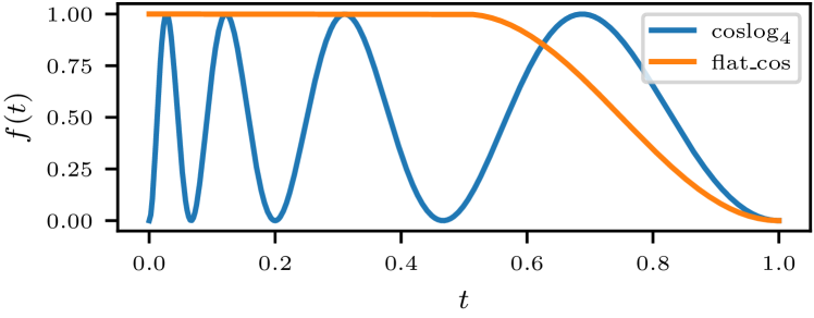
(b) The $\operatorname{coslog}_{4}$ and $\operatorname{flat\_cos}$ schedules.

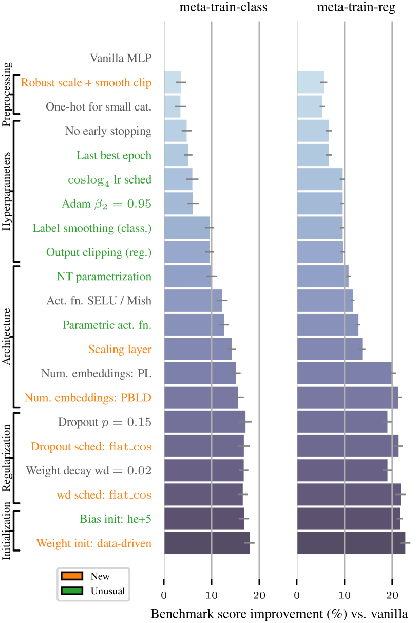
(c) From a vanilla MLP to RealMLP-TD.

Figure 1: Components of RealMLP-TD. In (c), we add one component in each step, tuning the best default learning rate for each step separately. The vanilla MLP uses categorical embeddings, a quantile transform to preprocess numerical features, default PyTorch initialization, ReLU activation, early stopping, and is optimized with Adam with default parameters. For more details, see Section A.3. The error bars are approximate 95% confidence intervals for the limit #splits $\to$ $\infty$, see Section C.5.

Data preprocessing

We first apply one-hot encoding to categorical columns with at most eight distinct values (not counting missing values). Binary categories are encoded to a single feature with values $\{-1,1\}$. Missing values in categorical columns are encoded to zero. We then preprocess all numerical columns, including the one-hot encoded ones, independently as follows: Let $x_{1},\ldots,x_{n}\in\mathbb{R}$ be the values in column $i$, and let $q_{p}$ be the $p$-quantile of $(x_{1},\ldots,x_{n})$ for $p\in[0,1]$. Then, +rCl+x* x_j,processed & ≔ f(s_j ⋅(x_j - q_1/2)),     f(x) ≔x1 + (x3)2,
s_j ≔ {1q3/4- q1/4, if q3/4≠q1/42q1- q0, if q3/4= q1/4 and q1≠q00 , otherwise. In scikit-learn [48], this corresponds to applying a RobustScaler (first case) or MinMaxScaler (second case), and then the function $f$, which smoothly clips its input to the range $(-3,3)$. Smooth clipping functions like $f$ have been used by, e.g., Holzmüller et al. [25] and Hafner et al. [21]. Intuitively, when features have large outliers, smooth clipping prevents the outliers from affecting the result too strongly, while robust scaling prevents the outliers from affecting the inlier scaling.

NN architecture

Our architecture, visualized in Figure 1 (a), is a multilayer perceptron (MLP) with three hidden layers containing 256 neurons each, except for the following additions and modifications:

• We use categorical embedding layers [20] to embed the remaining categorical features with cardinality $>8$.

• For numerical features, excluding the one-hot encoded ones, we introduce PBLD (periodic bias linear densenet) embeddings, which concatenate the original value to the PL embeddings proposed by Gorishniy et al. [17] and use a different periodic embedding with biases, inspired by [52]. PBLD embeddings apply separate small two-layer MLPs to each feature $x_{i}$ as +rCl+x* (x_i, W^(2,i)_emb cos(2πw^(1,i)_emb x_i + b^(1,i)_emb) + b^(2,i)_emb ) ∈R^4. For efficiency reasons, we use 4-dimensional embeddings with $\boldsymbol{w}^{(1,i)}_{\text{emb}},\boldsymbol{b}^{(1,i)}_{\text{emb}}\in\mathbb{R}^{16},\boldsymbol{b}^{(2,i)}_{\text{emb}}\in\mathbb{R}^{3},\boldsymbol{W}^{(2,i)}_{\text{emb}}\in\mathbb{R}^{3\times 16}$.

• To encourage (soft) feature selection, we introduce a scaling layer before the first linear layer, which is simply a matrix-vector product with a diagonal weight matrix. In other words, it computes $x_{i,\mathrm{out}}=s_{i}\cdot x_{i,\mathrm{in}}$, with a learnable scaling factor $s_{i}$ for each feature $i$. We found it beneficial to use a larger learning rate for this layer.

• Our linear layers use the neural tangent parametrization (NTP) as proposed by Jacot et al. [28], i.e., they compute $\boldsymbol{z}^{(l+1)}=d_{l}^{-1/2}\boldsymbol{W}^{(l)}\boldsymbol{x}^{(l)}+\boldsymbol{b}^{(l)}$, where $d_{l}$ is the dimension of the layer input $\boldsymbol{x}^{(l)}$. The motivation behind the use of the NTP here is that it effectively modifies the learning rate for the weight matrices depending on the input dimension $d_{l}$, hopefully preventing too large steps whenever the number of columns is large. We did not observe improvements when using the Adam version of the maximal update parametrization [67].

• We use parametric activation functions inspired by PReLU [22]. In general, for an activation function $\sigma$, we define a parametric version with separate learnable $\alpha_{i}$ for each neuron $i$: +rCl+x* σ_α_i(x_i) & = (1-α_i) x_i + α_i σ(x_i) . When $\alpha_{i}=1$, we recover $\sigma$, and when $\alpha_{i}=0$, the activation function is linear. As activation functions, we use SELU [35] for classification and Mish [45] for regression.

• We use dropout after each activation function. We do not use the Alpha-dropout variant originally proposed for SELU [35], as we were not able to obtain good results with it.

• For regression, at test time, we clip the MLP outputs to the observed range during training. (We observed that this is mainly helpful for suboptimal hyperparameters.)

Initialization

We initialize the parameters $s_{i}$ of the scaling layer to $1$, making it an identity function at initialization. We initialize the parameters $\alpha_{i}$ of the parametric activation functions to $1$, recovering the standard activation functions at initialization. We initialize weights and biases in a data-dependent fashion during a forward pass on the (possibly subsampled) training set. We rescale rows of standard-normal-initialized weight matrices to scale the variance of the output pre-activations over the dataset to one. For the biases, we use the data-dependent he+5 initialization method [60].

Training

We use the Adam optimizer [34] in the AdamW variant [40] for weight decay. We set its momentum hyperparameters to $\beta_{1}=0.9$ and $\beta_{2}=0.95$ instead of the default $\beta_{2}=0.999$. The idea to use a smaller value for $\beta_{2}$ is adopted from the fastai tabular MLP [26]. We optimize for 256 epochs with a batch size of 256. As a loss function for classification, we use softmax + cross-entropy with label smoothing [61] with parameter $\varepsilon=0.1$. To make the binary and multi-class cases more similar, we also use this loss function for binary classification instead of using a single output neuron with sigmoid and log-loss. For regression, we use the MSE loss and affinely transform the targets to have zero mean and unit variance on the training and validation set.

Hyperparameters

We allow parameter-specific scheduled hyperparameters computed in each iteration using a base value, optional parameter-specific factors, and a schedule, as +rCl+x* base_value ⋅ param_factor ⋅ schedule(iteration#iterations), allowing us, for example, to use a high learning rate factor for scaling layer parameters. Because we do not tune the number of epochs separately on each dataset, we use a multi-cycle learning rate schedule, providing multiple valleys that are usually preferable for stopping the training, while allowing high learning rates in between. Our schedule is similar to Loshchilov and Hutter [39] and Smith [58], but with a simpler analytical expression: +rCl+x* coslog_k(t) & ≔ 12(1 - cos(2πlog_2(1 + (2^k - 1)t))) . We set $k=4$ to obtain four cycles as shown in Figure 1 (b). To allow stopping at different levels of regularization, we schedule dropout and weight decay using the following schedule, cf. Figure 1 (b): +rCl+x* flat_cos(t) & ≔ 12 (1+cos(π(max{1,2t}-1))). The detailed hyperparameters can be found in Table A.1.

Best-epoch selection

Due to the multi-cycle learning rate schedule, we do not perform classical early stopping. Instead, we always train for the full 256 epochs and then revert the model to the epoch with the lowest validation error, which in this paper is based on classification error, or RMSE for regression. In case of a tie, we found it beneficial to use the last of the tied best epochs.

RealMLP-TD-S

Since certain aspects of RealMLP-TD are somewhat complex to implement, we introduce a simplified (and faster) variant called RealMLP-TD-S. Among the simplifications (see Appendix A) are: omitting embedding layers, using non-parametric activations, using a simpler initialization method, and omitting dropout and weight decay.

4 Gradient-Boosted Decision Trees

To find better default hyperparameters for GBDTs, we employ a semi-automatic approach: We use hyperparameter optimization libraries like hyperopt [2] and SMAC3 [38] to explore a reasonably large hyperparameter space, evaluating the benchmark score of each configuration on the meta-train benchmarks, and then perform some small manual adjustments like rounding the best obtained hyperparameters. To balance efficiency and accuracy, we fix the number of estimators to 1000 and use the hist method for XGBoost. We only consider the libraries’ default tree-building strategies since it is one of their main differences. The tuned defaults (TD) for LightGBM (LGBM), XGBoost (XGB), and CatBoost can be found in Table C.1, C.2, and C.3, respectively.

While some of the obtained hyperparameter values might be sensitive to the tuning and benchmark setup, we observe some general trends. First, row subsampling is applied in all settings, while column subsampling is rarely applied. Second, trees are generally allowed to be deeper for regression than for classification. Third, the Bernoulli bootstrap in CatBoost is competitive with the Bayesian bootstrap while also being faster.

5 Experiments

In the following, we evaluate different methods with library defaults (D), tuned defaults (TD), and hyperparameter optimization (HPO). Recall that TD uses fixed parameters optimized on the meta-train benchmarks, while HPO tunes hyperparameters on each dataset split independently. All methods except random forests select the best iteration/epoch on the validation set of the respective dataset split. All NN-based regression methods standardize the labels for training.

5.1 Methods

We use the following abbreviations, see Appendix C for more details:

• MLP-D, ResNet-D: MLP and ResNet from Gorishniy et al. [16] with default parameters from McElfresh et al. [43].

• TabR-S-D: TabR-S with default parameters [18], using context freeze for one slow dataset.

• RF-SKL-D: Random Forest [5] implementation of scikit-learn [48] with default parameters.

• CatBoost-D, LGBM-D, and XGB-D: CatBoost, LightGBM, and XGBoost defaults.

• XGB-PBB-D: XGBoost with optimized defaults (for AUC) from Probst et al. [50], using “hist” boosting.

• RealMLP-TD and RealMLP-TD-S: Our MLPs with tuned defaults from Section 3.

• CatBoost-TD, LGBM-TD, and XGB-TD: Tuned defaults for CatBoost, LightGBM, and XGBoost, respectively, as presented in Section 4.

• RealMLP-HPO, MLP-HPO, CatBoost-HPO, LGBM-HPO, and XGB-HPO: We apply 50 random search steps to each of the models, see Section C.2.

• Best-HPO, Best-TD, Best-D: Selecting the best model out of RealMLP, CatBoost, XGBoost, and LightGBM in the respective HPO, TD, or D variant based on the validation error on each dataset. For Best-D, we use MLP-D instead of RealMLP.

• Ensemble-HPO, Ensemble-TD, Ensemble-D: Similar to Best, but creating a weighted ensemble using the validation set as proposed by Caruana et al. [6], with 40 greedy selection steps as in Salinas and Erickson [54].

5.2 Results

Figure 2 shows the results of the aforementioned methods on the meta-train and meta-test benchmarks, along with their runtimes on a CPU. We also show results for the benchmark of [19] in Figure 3, specifically the version with medium-size datasets ($\leq 10$K training samples). The latter include scikit-learn’s GradientBoostingTree (GBT-SKL) as well as two transformer-based models, FT-Transformer [16] and SAINT [59]. For the baselines, we use (slightly adapted) HPO search spaces from the original paper, see Section C.4.

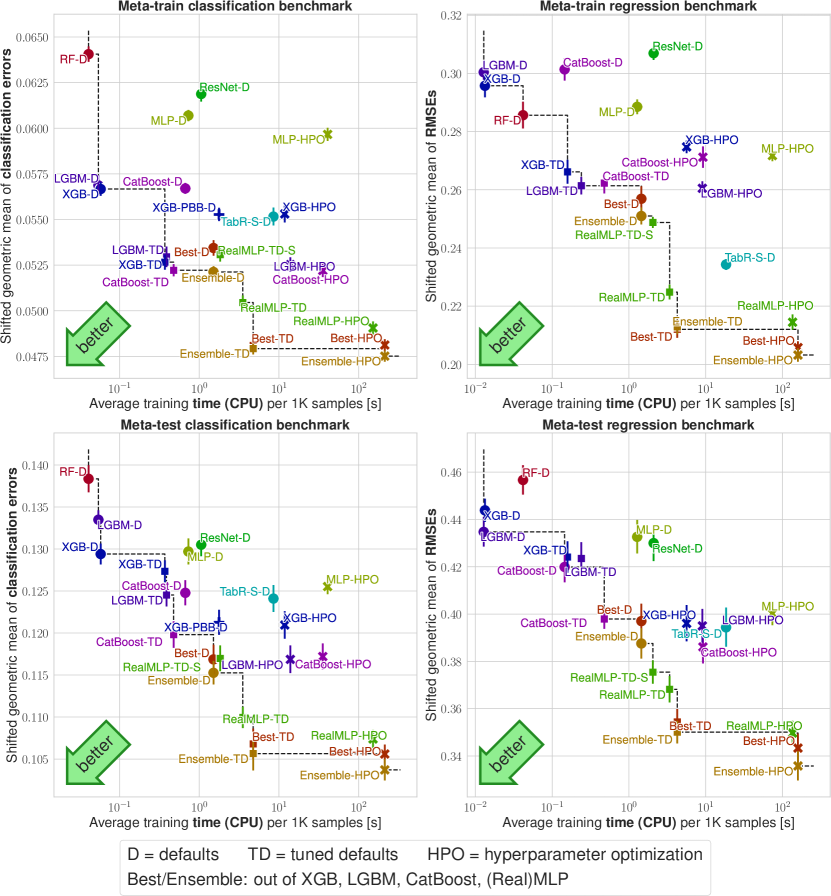
Figure 2: Benchmark scores on $\mathcal{B}^{\operatorname{train}}_{\mathrm{class}}$, $\mathcal{B}^{\operatorname{train}}_{\mathrm{reg}}$, $\mathcal{B}^{\operatorname{test}}_{\mathrm{class}}$, and $\mathcal{B}^{\operatorname{test}}_{\mathrm{reg}}$ vs. average training time. The $y$-axis shows the shifted geometric mean ($\operatorname{SGM}_{\varepsilon}$) classification error (left) or RMSE (right) as explained in Section 2.2. The $x$-axis shows average training times per 1000 samples (measured on $\mathcal{B}^{\operatorname{train}}$ for efficiency reasons), see LABEL:sec:appendix:runtimes. The error bars are approximate 95% confidence intervals for the limit #splits $\to$ $\infty$, see Section C.5.

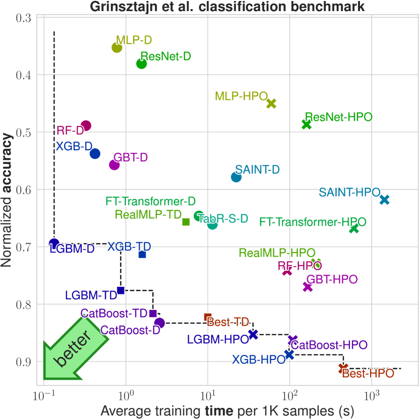
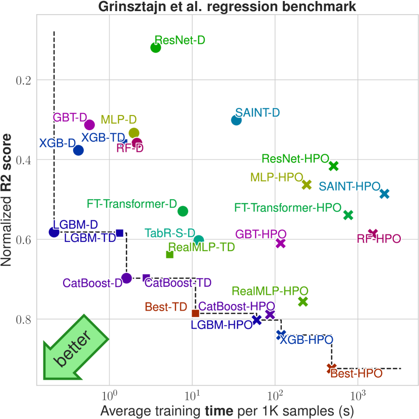
Figure 3: Results on the benchmarks of Grinsztajn et al. [19]. The $y$-axis (inverted) shows the normalized accuracy / R2 score used in the original paper (see Section C.4). The $x$-axis shows average training times per 1000 samples, using GPUs for NNs as in [19], see LABEL:sec:appendix:runtimes.

How good are tuned defaults on new datasets?

To answer this question, we compare the relative gaps between TD and HPO benchmark scores on the meta-test benchmarks to those on the meta-train benchmarks. The gap between RealMLP-HPO and RealMLP-TD is about equally large on the meta-train and meta-test benchmarks, indicating that the tuned defaults transfer very well to the meta-test benchmark. For GBDTs, tuned defaults are competitive with HPO on the meta-train set, but not as good on the meta-test set. Still, they are considerably better than the untuned defaults on the meta-test set. Note that we did not limit the TD parameters to the literature search spaces for the HPO models (cf. Section C.2); for example, XGB-TD uses a smaller value of min_child_weight for classification and CatBoost-TD uses deeper trees and Bernoulli boosting. The XGBoost defaults XGB-PBB-D from Probst et al. [50] outperform XGB-TD on $\mathcal{B}^{\operatorname{test}}_{\mathrm{class}}$, perhaps because their benchmark is more similar to $\mathcal{B}^{\operatorname{test}}_{\mathrm{class}}$ or because XGB-PBB-D uses more estimators (4168) and deeper trees.

Among GBDTs, CatBoost defaults are better and slower.

Several papers have found CatBoost to perform favorably among GBDTs while being more computationally expensive to train [51, 43, 9, 33, 68]. We observe the same for our tuned defaults on the meta-test benchmark.

RealMLP performs favorably among NNs.

We can see on the meta-test benchmark as well as the benchmark by [19] that RealMLP-TD performs significantly better than MLP-D and ResNet-D. RealMLP-TD is slower on average, mainly due to the use of numerical embeddings and the lack of early stopping. However, the latter allows efficient cross-validation and ensemble training through vectorization. On the benchmark by [19], RealMLP-TD achieves equal or better results than other NNs, and in the HPO setting, it outperforms transformer-based models in terms of speed and benchmark scores. In addition, RealMLP-TD is faster than TabR-S-D while also achieving better meta-test benchmark scores. When looking at rank-based metrics in Appendix B, RealMLP-TD is worse than TabR-S-D on $\mathcal{B}^{\operatorname{train}}_{\mathrm{reg}}$ but better on $\mathcal{B}^{\operatorname{train}}_{\mathrm{class}}$ and $\mathcal{B}^{\operatorname{test}}_{\mathrm{class}}$.

NN improvements

Figure 1 (c) shows how adding the proposed RealMLP components to a simple MLP improves the meta-train benchmark performance. However, these results depend on the order in which components are added, which is addressed by a separate ablation study in Appendix B. We also show in Section B.7 that our architectural improvements alone are beneficial when applied to MLP-D directly, although non-architectural aspects are at least as important. In particular, our numerical preprocessing is easy to adopt and often beneficial for other NNs as well.

RealMLP is competitive with tree-based models.

On the meta-test benchmark, in the TD and HPO setting, our MLP performs better than GBDTs in terms of shifted geometric mean error. When considering arithmetic mean error and average rank, RealMLP is comparable to or slightly better than GBDTs (Section B.9). The improvement in shifted geometric mean error reflects the fact that on several datasets, the NN has a lower error by roughly an order of magnitude. The win rate of RealMLP-TD vs. CatBoost-TD is around 51–62% and the win rate of RealMLP-HPO vs. CatBoost-HPO is around 55–60% (Section B.11). On the benchmark of [19], RealMLP performs worse for classification but comparably for regression.

Simply trying all default algorithms is very often better than (naive) single-algorithm HPO, and always faster.

When comparing Best-TD to 50-step HPO on any individual algorithm, we notice that Best-TD is always faster, while also being better on the meta-train and meta-test benchmarks and only slightly worse than the best HPO models on the benchmark of [19]. We also note that ensemble selection [6] usually gives 1–3% improvement on the benchmark score compared to selecting the best model, and can potentially be further improved [7]. Our results indicate that our methods have the potential to be useful within AutoML methods, which may implement more sophisticated methods such as training-time-aware HPO or stacking. We note that this surprising performance directly results from the quality of our tuned default hyperparameters and RealMLP, as selecting or ensembling non-tuned defaults is matched by LGBM-HPO and outperformed by RealMLP-HPO (Figure 2).

Further insights

In Appendix B, we present further experimental results, including an ablation study. We compare bagging and refitting for RealMLP-TD and LGBM-TD, finding that refitting multiple models is often better on average. We demonstrate that GBDTs benefit from high early stopping patiences for classification, especially when using accuracy as the stopping metric. When considering ROC AUC as a stopping metric, we show that stopping on cross-entropy is preferable to accuracy, and that label smoothing is harmful. We also investigate robust scaling and smooth clipping for other NNs, showing that it is often helpful.

Limitations

In our benchmarks, we have considered medium-to-large tabular datasets with random train-test splits, using classification error and RMSE as metrics, with additional results for AUROC in Section B.5. It is unclear to which extent the obtained defaults can generalize to very small datasets, distribution shifts, datasets with missing numerical values, and other metrics such as log-loss. Additionally, runtimes and the resulting tradeoffs may change with different parallelization, different (time-aware) HPO algorithms, or different hardware. For computational reasons, we only use a single training-validation split per train-test split. This means that HPO can overfit the validation set more easily than in a cross-validation setup. While we extensively benchmark different NN models from the literature, we do not attempt to equalize non-architectural aspects, and our work should therefore not be seen as a comparison of architectures. We compared to TabR-S-D as a recent promising method with good default parameters [18, 68]. However, due to a surge of recently published deep tabular models [e.g., 8, 9, 56, 41, 33, 66, 29], it is unclear what the current “best” deep tabular model is.

6 Conclusion

In this paper, we studied the potential of improved default parameters for GBDTs and an improved MLP, evaluated on a large separate meta-test benchmark as well as the benchmark by [19], and investigated the time-accuracy tradeoffs of various algorithm selection and ensembling scenarios. Our improved MLP mostly outperforms other NNs from the literature with moderate runtime and is competitive with GBDTs. Since many of the proposed improvements to NNs are orthogonal to the improvements in other papers, they offer exciting opportunities for combinations. While the “NNs vs GBDTs” debate remains interesting, our results demonstrate that with good default parameters, it is worth trying both algorithm families even with a moderate training time budget.

Appendix A Further Details on RealMLP-TD and RealMLP-TD-S

The detailed hyperparameter settings for RealMLP-TD and RealMLP-TD-S are listed in Table A.1.

Table A.1: Overview of hyperparameters for RealMLP-TD and RealMLP-TD-S.

	RealMLP-TD		RealMLP-TD-S
Hyperparameter	classification	regression	classification	regression
Num. embedding type	PBLD	PBLD	None	None
Num. embedding periodic init std.	0.1	0.1	—	—
Num. embedding hidden dimension	16	16	—	—
Num. embedding dimension	4	4	—	—
Max one-hot size (without missing)	8	8	$\infty$	$\infty$
Num. preprocessing	robust scale + smooth clip
Categorical embedding dimension	8	8	—	—
Categorical embedding initialization	$\mathcal{N}(0,1)$	$\mathcal{N}(0,1)$	—	—
Use scaling layer	yes
Scaling layer initialization	1.0 (constant)
Number of linear layers	4
Hidden layer sizes	[256, 256, 256]
Activation function	SELU	Mish	SELU	Mish
Use parametric activation function	yes	yes	no	no
Parametric activation function initialization	1.0	1.0	—	—
Linear layer parametrization	NTP
Last linear layer weight initialization	data-driven	data-driven	zero	zero
Other linear layer weight initialization	data-driven	data-driven	std normal	std normal
Last linear layer bias initialization	he+5	he+5	zero	zero
Other linear layer bias initialization	he+5	he+5	std normal	std normal
Optimizer	AdamW
Batch size	256
Number of epochs	256
Adam $\beta_{1}$	0.9
Adam $\beta_{2}$	0.95
Adam $\varepsilon$	1e-8
Learning rate (base value)	0.04	0.2	0.04	0.07
Learning rate schedule	$\operatorname{coslog}_{4}$
Learning rate (num. emb. factor)	0.1	0.1	—	—
Learning rate (scaling layer factor)	6
Learning rate (bias factor)	0.1
Learning rate (param. act. factor)	0.1	0.1	—	—
Dropout probability (base value)	0.15	0.15	0.0	0.0
Dropout schedule	$\operatorname{flat\_cos}$	$\operatorname{flat\_cos}$	—	—
Weight decay (base value)	0.02	0.02	0.0	0.0
Weight decay schedule	$\operatorname{flat\_cos}$	$\operatorname{flat\_cos}$	—	—
Weight decay (bias factor)	0.0	0.0	—	—
Loss function	cross-entropy	MSE	cross-entropy	MSE
Label smoothing $\varepsilon$	0.1	—	0.1	—
Standardize targets during training	—	yes	—	yes
Output min-max clipping	—	yes	—	no
Best epoch selection metric	class. error	MSE	class. error	MSE
Best epoch selection method	last best validation error

A.1 RealMLP-TD Details

Initialization

We initialize categorical embedding parameters from $\mathcal{N}(0,1)$. We initialize the components of $\boldsymbol{w}^{(1,i)}_{\text{emb}}$ from $\mathcal{N}(0,0.1^{2})$ and of $\boldsymbol{b}^{(1,i)}_{\text{emb}}$ from $\mathcal{U}[-\pi,\pi]$. The other numerical embedding parameters are initialized according to PyTorch’s default initialization, that is, from the uniform distribution $\mathcal{U}[-1/\sqrt{16},1/\sqrt{16}]$. For weights and biases of the linear layers, we use a data-dependent initialization. The initialization is performed on the fly during a first forward pass of the network on the training set (which can be subsampled adaptively not to use more than 1 GB of RAM). We realize this by providing fit_transform() methods similar to a pipeline in scikit-learn. For the weight matrices, we use a custom two-step procedure: First, we initialize all entries from $\mathcal{N}(0,1)$. Then, we rescale each row of the weight matrix such that the outputs $\frac{1}{\sqrt{d_{l}}}\boldsymbol{W}^{(l)}\boldsymbol{x}_{j}^{(l)}$ have variance $1$ over the dataset (i.e. when considering the sample index $j\in\{1,\ldots,n\}$ as a uniformly distributed random variable). This is somewhat similar to the LSUV initialization method [44]. For the biases, we use the data-dependent he+5 initialization method [60].

Training

We implement weight decay as in PyTorch using $\theta\leftarrow\theta-\text{lr}\cdot\text{wd}\cdot\theta$, which includes the learning rate unlike the original version [40].

A.2 RealMLP-TD-S Details

For RealMLP-TD-S, we make the following changes compared to RealMLP-TD:

• We apply one-hot encoding to all categorical variables and do not apply categorical embeddings.

• We do not apply numerical embeddings.

• We use the standard non-parametric versions of the SELU and Mish activation functions.

• We do not use dropout and weight decay.

• We use simpler weight and bias initializations: We initialize weights and biases from $\mathcal{N}(0,1)$, except in the last layer, where we initialize them to zero.

• We do not clip the outputs, even in the regression case.

• We apply a different base learning rate in the regression case.

A.3 Details on Cumulative Ablation

Here, we provide more details on the vanilla MLP and the ablation steps from Figure 1 (c). For each step, we choose the best default learning rate out of a learning rate grid, using $\{0.0004,0.0007,0.001,0.0015,0.0025,0.004,0.007,0.01,0.015\}$ for NNs using standard parametrization and $\{0.01,0.02,0.03,0.04,0.07,0.1,0.2,0.3,0.4\}$ for NNs using neural tangent parametrization.

• Vanilla MLP: We use three hidden layers with 256 hidden neurons in each layer, just like RealMLP-TD, and the ReLU activation function. Each linear layer uses standard parametrization and the PyTorch default initialization, which is uniform from $[-1/\sqrt{\text{fan\_in}},1/\sqrt{\text{fan\_in}}]$ for both weights and biases, where fan_in is the input dimension. Categorical features are embedded using embedding layers, using eight-dimensional embeddings for each feature. Numerical features are transformed using a scikit-learn QuantileTransformer to approximately normal-distributed features. Optimization is performed using Adam with constant learning rate and default parameters $\beta_{1}=0.9,\beta_{2}=0.999,\varepsilon=10^{-8}$ for at most 256 epochs with batch size 256, with constant learning rate. If the best validation error (classification error or RMSE) does not improve for 40 epochs, training is stopped. In each case, the model is reverted to the parameters of the epoch with the best validation score, using the first best epoch in case of a tie.

• Robust scale + smooth clip: We replace the QuantileTransformer with robust scaling and smooth clipping.

• One-hot for small cat.: As in RealMLP-TD, we use one-hot encoding for categories with at most eight values, not counting missing values.

• No early stopping: We always train the full 256 epochs.

• Last best epoch: In case of a tie, we use the last of the best epochs.

• $\operatorname{coslog}_{4}$ lr sched: We use the $\operatorname{coslog}_{4}$ learning rate schedule instead of a constant one.

• Adam $\beta_{2}=0.95$: We set $\beta_{2}=0.95$.

• Label smoothing (class.): We enable label smoothing with $\varepsilon=0.1$ in the classification case.

• Output clipping (reg.): For regression, outputs are clipped to the min-max range observed during training.

• NT parametrization: We use the neural tangent parametrization for linear layers, setting the bias learning rate factor to $0.1$.

• Act. fn. SELU / Mish: We change the activation function from ReLU to SELU (classification) or Mish (regression).

• Parametric act. fn.: We use parametric versions of the activation functions, with a learning rate factor of $0.1$ for the parameters.

• Scaling layer: We use a scaling layer with a learning rate factor of $6$ before the first linear layer.

• Num. embeddings: PL: We apply the PL embeddings [17] to numerical features.

• Num. embeddings: PBLD: We apply our PBLD embeddings instead.

• Dropout $p=0.15$: We apply dropout with probability $0.15$.

• Dropout sched: $\operatorname{flat\_cos}$: We apply the $\operatorname{flat\_cos}$ schedule to the dropout probability.

• Weight decay wd $=$ $0.02$: We apply weight decay (as in AdamW, PyTorch version) with value $0.02$.

• wd sched: $\operatorname{flat\_cos}$: We apply the $\operatorname{flat\_cos}$ schedule to weight decay.

• Bias init: he+5: We apply the he+5 bias initialization method from [60].

• Weight init: data-driven: We apply our data-driven weight initialization method.

A.4 Discussion

Here, we discuss some of the design decisions behind RealMLP-TD and possible trade-offs. First, our implementation allows us to train RealMLP-TD in a vectorized fashion on multiple train-validation-test splits at the same time. On the one hand, this can lead to speedups on GPUs when training multiple models in parallel, including on the benchmarks. On the other hand, it can hinder the implementation of certain methods like patience-based early stopping or loss-based learning rate schedules. While our ablations in Section B.1 show the advantage of our multi-cycle schedule over decreasing learning rate schedules, the latter ones could potentially enable a faster average training time through low-patience early stopping. An interesting follow-up question could be whether the multi-cycle schedule still works well with larger-patience early stopping.

Regarding categorical embeddings, our meta-train benchmark does not contain many high-cardinality categorical variables, and we were not able to conclude whether categorical embeddings are helpful or harmful compared to one-hot encoding (see Section B.1). Our motivation to include categorical embeddings stems from [20] as well as their potential to be more efficient for high-cardinality categorical variables. However, in practice, we find pure one-hot encoding to be faster on most datasets. Regarding the embedding size, we found that 4 already gave good results for numerical embeddings and decided to use 8 for categorical variables.

Additionally, other speed-accuracy tradeoffs are possible. Especially for regression, we observed that more epochs and larger hidden layers can be helpful. When faster networks are desired, the omission of numerical and categorical embedding layers as well as parametric activations from RealMLP-TD can be helpful, while the other omissions in RealMLP-TD-S do not considerably affect the training time. Of course, using larger batch sizes can also be helpful for larger datasets.

One caveat for classification is that cross-entropy with label smoothing is not a proper scoring rule, that is, in the infinite-sample limit, it is not minimized by the true probabilities $P(y|x)$ [15]. Hence, label smoothing might not be suitable when other classification error metrics are used, as demonstrated in Section B.5 for AUROC.

Appendix B More Experiments

B.1 MLP Ablations

To assess the importance of different improvements in RealMLP-TD, we perform an ablation study. We perform the ablation study only on the meta-train benchmarks, first because they are considerably faster to run, and second because we tune the default parameters only on the meta-train benchmarks. Since the hyperparameters of RealMLP-TD have been tuned on the meta-train benchmarks, the ablation scores are not unbiased but represent some of the considerations that have been made when tuning the defaults. For each ablation, we multiply the default learning rate by learning rate factors from the grid $\{0.1,0.15,0.25,0.35,0.5,0.7,1.0,1.4,2.0,3.0,4.0\}$ and pick the best one. Table B.1 shows the results of the ablation study in terms of the relative increase of the benchmark score for each ablation.

In general, we observe that ablations often lead to much larger changes for regression than for classification. Perhaps this is because RMSE is more sensitive compared to classification error. Another factor could be that the classification benchmark contains more datasets than the regression benchmark. For the specific ablations, we observe a few things:

• For the numerical embeddings, we see that PBLD outperforms PL, PLR, and no numerical embeddings. Contrary to Gorishniy et al. [17], PL embeddings perform better than PLR embeddings in our setting. While the configurations with PLR and no numerical embeddings appear extremely bad for regression, we observed that they can perform more benignly with lower weight decay values.

• Using the Adam default value of $\beta_{2}=0.999$ instead of our default $\beta_{2}=0.95$ leads to considerably worse performance, especially for regression. As for numerical embeddings, we observed that the difference is less pronounced at lower weight decay values.

• Using a cosine decay learning rate schedule instead of our multi-cycle schedule leads to small deteriorations. A constant learning rate schedule performs even worse, especially for regression.

• Not employing label smoothing for classification is detrimental by around 1.8%.

• The learnable scaling layer yields improvements around 1.2% on both benchmarks.

• The use of parametric activations results in a considerable 4.8% improvement for regression but is insignificant for classification. We observed that parametric activations can sometimes alleviate optimization difficulties with weight decay.

• The differences between activation functions are rather small. For classification, Mish is competitive with SELU in this ablation but we found it to be worse in some other hyperparameter settings, so we keep SELU as the default. For regression, Mish performs best.

• For dropout and weight decay, we observe that they yield comparable but not always significant benefits for classification and regression. Scheduling dropout and weight decay parameters with the $\operatorname{flat\_cos}$ schedule is helpful for regression, but not for classification in this setting.

• When comparing the standard parametrization (SP) to the neural tangent parametrization (NTP), we disable weight decay for a fair comparison. Moreover, for SP, we set the learning rate factors for weight and bias layers to $1/16=1/\sqrt{256}$. This is because, for the weights in NTP, the effective updates by Adam are damped by this factor in all hidden layers except the first one. Compared to NTP without weight decay, SP without weight decay performs insignificantly worse on both benchmarks. It is unclear to us why the parametrization, which has a considerable influence on how the effective learning speed of the first linear layer scales with the number of features, is apparently of little importance.

• When comparing the data-dependent initialization of RealMLP-TD to a vanilla initialization with standard normal weights and zero biases, we see that the data-dependent initialization gains around 1% on both benchmarks.

• For selecting the best epoch, we consider selecting the first best epoch instead of the last best epoch in case of a tie. This is only relevant for classification metrics like classification error, where ties are somewhat likely to occur, especially on small and “easy” datasets. We observe a non-significant 0.4% deterioration in the benchmark score.

• We do not observe a significant difference when using one-hot encoding for all categorical variables, since our benchmarks contain only very few datasets with large-cardinality categorical variables.

Table B.1: Ablation experiments for RealMLP-TD. We re-tune the learning rate (picking the one with the best $\operatorname{SGM}_{\varepsilon}$ benchmark score) for each ablation separately. For each ablation, we specify the increase in the benchmark score ($\operatorname{SGM}_{\varepsilon}$) relative to RealMLP-TD, with approximate 95% confidence intervals (Section C.5), and the best learning rate factor found. In the cases where values are missing, the corresponding option is already the default.

	meta-train-class		meta-train-reg
Ablation	Error increase in %	best lr factor	Error increase in %	best lr factor
MLP-TD (without ablation)	0.0 [0.0, 0.0]	1.0	0.0 [0.0, 0.0]	1.0
Num. embeddings: PL	0.7 [-0.0, 1.4]	1.0	0.5 [-0.5, 1.6]	1.0
Num. embeddings: PLR	4.2 [2.8, 5.7]	1.0	19.0 [13.7, 24.5]	0.25
Num. embeddings: None	2.3 [1.7, 2.9]	1.0	20.6 [19.4, 21.8]	0.25
Adam $\beta_{2}=0.999$ instead of $\beta_{2}=0.95$	2.0 [1.6, 2.4]	2.0	22.8 [21.3, 24.4]	0.35
Learning rate schedule = cosine decay	1.1 [0.6, 1.5]	1.0	0.4 [-0.5, 1.2]	3.0
Learning rate schedule = constant	1.8 [0.9, 2.8]	0.25	13.4 [11.9, 15.0]	0.15
No label smoothing	1.8 [1.2, 2.5]	4.0
No learnable scaling	1.4 [0.7, 2.1]	2.0	1.0 [-0.0, 2.0]	2.0
Non-parametric activation	0.5 [-0.2, 1.2]	3.0	4.8 [3.4, 6.2]	0.35
Activation=Mish	-0.0 [-0.6, 0.6]	3.0
Activation=ReLU	0.5 [-0.1, 1.2]	2.0	0.7 [-0.1, 1.6]	1.0
Activation=SELU			2.3 [1.1, 3.6]	1.0
No dropout	0.8 [0.2, 1.3]	3.0	0.8 [-0.5, 2.1]	1.4
Dropout prob. $0.15$ (constant)	-0.1 [-1.0, 0.8]	1.4	3.6 [3.0, 4.2]	1.0
No weight decay	0.8 [-0.2, 1.8]	0.5	0.9 [-0.1, 1.9]	0.5
Weight decay = 0.02 (constant)	-0.3 [-0.7, 0.1]	3.0	3.1 [1.7, 4.4]	1.4
Standard param + no weight decay	1.1 [0.2, 2.1]	0.5	1.3 [0.7, 1.8]	0.7
No data-dependent init	0.9 [0.1, 1.8]	3.0	1.2 [0.2, 2.2]	1.4
First best epoch instead of last best	0.4 [-0.1, 1.0]	4.0	0.0 [-0.0, 0.0]	1.0
Only one-hot encoding	-0.0 [-0.1, 0.0]	1.0	0.0 [-0.0, 0.0]	1.0

B.2 MLP Preprocessing

In Table B.2, we compare different preprocessing methods for numerical features. Since we want to compare these methods in a relatively conventional setting, we apply them to RealMLP-TD-S (without numerical embeddings) and before one-hot encoding. We compare the following methods:

• Robust scaling and smooth clipping, our method used in RealMLP-TD and RealMLP-TD-S and described in Section 3.

• Robust scaling without smooth clipping.

• Standardization, i.e. subtracting the mean and dividing by the standard deviation. If the standard deviation of a feature is zero, we set the feature to zero.

• Standardization followed by smooth clipping.

• The quantile transformation from scikit-learn [48] with normal output distribution, which is popular in recent works [19, 17, 18, 43].

• A variant of the quantile transform, which we call the RTDL version, used by [16] and [18]. This version uses a dataset size dependent number of quantiles and adds some noise before fitting the transformation.

• The recent kernel density integral transform [42], which interpolates between the quantile transformation and min-max scaling, with default parameter $\alpha=1$.

Table B.2 shows that on the meta-train benchmark, robust scaling and smooth clipping performs best for both classification and regression.

Table B.2: Effects of different preprocessing methods for numerical features for RealMLP-TD-S. We report the relative increase in the shifted geometric mean benchmark scores compared to the standard method used in RealMLP-TD and RealMLP-TD-S, which is robust scaling and smooth clipping. We also report approximate 95% confidence intervals. To have a more common setting, we do not apply the preprocessing methods to one-hot encoded categorical features. In each column, the best score is highlighted in bold, and errors whose confidence interval contains the best score are underlined.

	Error increase relative to robust scale + smooth clip in %
Method	meta-train-class	meta-train-reg
Robust scale + smooth clip	0.0 [0.0, 0.0]	0.0 [0.0, 0.0]
Robust scale	0.5 [-0.4, 1.4]	9.5 [4.4, 14.8]
Standardize + smooth clip	1.6 [0.9, 2.2]	1.2 [0.6, 1.8]
Standardize	2.1 [1.2, 3.0]	8.7 [3.9, 13.9]
Quantile transform (output dist. = normal)	2.3 [1.5, 3.2]	6.3 [5.5, 7.0]
Quantile transform (RTDL version)	2.6 [1.5, 3.7]	2.6 [0.4, 4.8]
KDI transform ($\alpha=1$, output dist. = normal)	4.9 [3.8, 6.0]	4.4 [2.6, 6.2]

B.3 Bagging, Refitting, and Ensembling

In our benchmark, for each training-test split, we only train one model on one training-validation split for efficiency reasons. However, ensembling and cross-validation techniques usually allow additional improvements to models. Here, we study multiple variants for RealMLP-TD and LGBM-TD. Let $\mathcal{D}$ be the available data for training and validation, split into five equal-size subsets $\mathcal{D}_{1},\ldots,\mathcal{D}_{5}$. (When $|\mathcal{D}|$ is not divisible by five, $\mathcal{D}_{1}\cup\ldots\cup\mathcal{D}_{5}\subsetneq\mathcal{D}$ since we need equal-size validation sets for vectorized NNs.) Let $f_{\mathcal{D},t}(X)$ be the predictions on inputs $X$ of the model trained on training set $\mathcal{D}$ after $t\in\{1,\ldots,T\}$ epochs (for NNs) or iterations (for LGBM). For classification, we consider the class probabilities as predictions. Let $L_{\mathcal{D}^{\prime}}(f_{\mathcal{D},t})$ be the loss of $f_{\mathcal{D},t}$ on dataset $\mathcal{D}^{\prime}$. Then, we compare the test errors of an ensemble of $M=1$ or $M=5$ models, trained using bagging or refitting, with individual or joint stopping (best-epoch selection), which is formally given as follows:

+rCl+x* y_pred& ≔ 1M ∑_i=1^M f_~D_i, t_i^*(X_test),  (M models)
~D_i ≔ {D∖Di(bagging)D(refitting),
t_i^* ≔ {argmint ∈{1, …, T}LDi(fD∖Di, t) (indiv. stopping)argmint ∈{1, …, T}∑j=15LDj(fD∖Dj, t) (joint stopping).

Here, each model is trained with a different random seed. For LGBM, since we use an early stopping patience of 300 for each of the individual models, the $\operatorname*{argmin}$ in the definition of $t_{i}^{*}$ can only go up to the minimum stopping iteration $T$ across the considered models.

Table B.3: Improvements for LGBM-TD by bagging or (ensembled) refitting. We perform 5-fold cross-validation, stratified for classification, and 5-fold refitting. We compare compare bagging vs. refitting, one model vs. five models, and individual stopping vs. joint stopping. The table shows the relative reduction in shifted geometric mean benchmark scores, including approximated 95% confidence intervals (Section C.5). In each column, the best score is highlighted in bold, and errors whose confidence interval contains the best score are underlined.

	Error reduction relative to 1 fold in %
Method	meta-train-class	meta-test-class	meta-train-reg	meta-test-reg
LGBM-TD (bagging, 1 model, indiv. stopping)	-0.0 [-0.0, -0.0]	-0.0 [-0.0, -0.0]	-0.0 [-0.0, -0.0]	-0.0 [-0.0, -0.0]
LGBM-TD (bagging, 1 model, joint stopping)	0.0 [-0.2, 0.2]	-0.6 [-1.1, -0.2]	-0.0 [-0.1, 0.0]	0.2 [-0.1, 0.6]
LGBM-TD (bagging, 5 models, indiv. stopping)	3.7 [3.1, 4.4]	4.4 [3.8, 5.0]	3.9 [2.2, 5.6]	4.2 [3.6, 4.8]
LGBM-TD (bagging, 5 models, joint stopping)	3.5 [2.8, 4.2]	3.6 [3.0, 4.2]	3.9 [2.2, 5.5]	4.2 [3.7, 4.8]
LGBM-TD (refitting, 1 model, indiv. stopping)	5.2 [4.5, 5.8]	1.7 [-0.5, 3.9]	2.4 [-0.1, 4.9]	4.2 [3.6, 4.8]
LGBM-TD (refitting, 1 model, joint stopping)	5.3 [4.8, 5.9]	4.7 [3.9, 5.5]	2.4 [-0.0, 4.7]	4.2 [3.7, 4.8]
LGBM-TD (refitting, 5 models, indiv. stopping)	6.0 [5.4, 6.5]	6.3 [5.2, 7.5]	3.8 [1.6, 6.0]	5.7 [5.1, 6.3]
LGBM-TD (refitting, 5 models, joint stopping)	5.8 [5.2, 6.4]	6.2 [5.4, 7.1]	3.9 [1.6, 6.1]	5.6 [5.1, 6.1]

Table B.4: Improvements for RealMLP-TD by bagging or (ensembled) refitting. We perform 5-fold cross-validation, stratified for classification, and 5-fold refitting. We compare bagging vs. refitting, one model vs. five models, and individual stopping vs. joint stopping. The table shows the relative reduction in shifted geometric mean benchmark scores, including approximated 95% confidence intervals (Section C.5). In each column, the best score is highlighted in bold, and errors whose confidence interval contains the best score are underlined.

	Error reduction relative to 1 fold in %
Method	meta-train-class	meta-test-class	meta-train-reg	meta-test-reg
RealMLP-TD (bagging, 1 model, indiv. stopping)	-0.0 [-0.0, -0.0]	-0.0 [-0.0, -0.0]	-0.0 [-0.0, -0.0]	-0.0 [-0.0, -0.0]
RealMLP-TD (bagging, 1 model, joint stopping)	1.1 [0.0, 2.2]	0.7 [0.2, 1.2]	0.5 [0.2, 0.8]	0.8 [-0.5, 2.1]
RealMLP-TD (bagging, 5 models, indiv. stopping)	6.2 [5.2, 7.2]	8.0 [7.3, 8.7]	6.6 [6.0, 7.1]	4.9 [4.3, 5.6]
RealMLP-TD (bagging, 5 models, joint stopping)	6.2 [5.3, 7.1]	7.6 [6.7, 8.5]	6.5 [5.9, 7.1]	4.6 [3.7, 5.4]
RealMLP-TD (refitting, 1 model, indiv. stopping)	2.2 [1.2, 3.3]	3.5 [2.4, 4.7]	2.6 [1.6, 3.5]	1.0 [0.0, 2.0]
RealMLP-TD (refitting, 1 model, joint stopping)	4.8 [3.9, 5.6]	5.0 [4.2, 5.8]	4.3 [3.3, 5.4]	2.4 [1.2, 3.5]
RealMLP-TD (refitting, 5 models, indiv. stopping)	7.1 [6.4, 7.7]	9.1 [8.3, 9.8]	8.3 [7.6, 9.0]	5.1 [4.2, 6.0]
RealMLP-TD (refitting, 5 models, joint stopping)	7.7 [6.9, 8.6]	8.9 [8.3, 9.4]	8.5 [7.8, 9.2]	5.5 [4.6, 6.4]

The results of our experiments can be found in Table B.3 for LGBM-TD and in Table B.4 for RealMLP-TD. As expected, five models are considerably better than one. We find that refitting is mostly better than bagging, although a disadvantage of refitted models is that no validation scores are available, and it is unclear how HPO would affect this comparison. Comparing individual stopping to joint stopping, we find that individual stopping has a slight advantage in five-model bagging, while joint stopping performs better for single-model refitting. In the other two scenarios, joint stopping appears slightly better for RealMLP-TD and slightly worse for LGBM-TD. We also observe that the benefit of using five models instead of one appears to be larger for RealMLP-TD than for LGBM-TD.

B.4 Early stopping for GBDTs

In Figure B.1 and Figure B.2, we study the influence of different early stopping patiences and metrics on the resulting benchmark performance of XGB-TD, LGBM-TD, and CatBoost-TD. While the regression results only deteriorate slightly for low patiences of 10 or 20 iterations, classification results are much more hurt by low patiences. In the classification setting, we evaluate the use of different losses for early stopping and for best-epoch selection: classification error, Brier score, and cross-entropy loss. In each case, cross-entropy loss is used as the training loss, and classification error is used for evaluating the models on the test sets in the computation of the benchmark score. We observe that models stopped on classification error strongly deteriorate at low patiences ($\lesssim 100$), while our default patience of 300 achieves close-to-optimal results. Models stopped on cross-entropy loss deteriorate much less at low patiences, but achieve roughly 2% worse benchmark score at high patiences. Stopping on Brier loss achieves very good high-patience performance and is still only slightly more sensitive to the patience than stopping on cross-entropy loss. An interesting follow-up question would be if HPO can attenuate the differences between different settings.

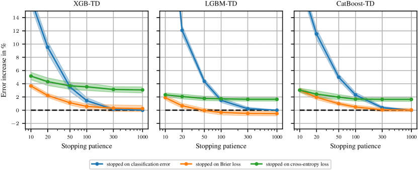
Figure B.1: Effect of stopping patiences and metrics on the performance of GBDTs on $\mathcal{B}^{\operatorname{train}}_{\mathrm{class}}$. We run the XGB-TD, LGBM-TD, and CatBoost-TD with different early stopping patiences (early_stopping_rounds). We compare three different metrics used for stopping and best-epoch selection: classification error, Brier loss, and cross-entropy loss. The $y$-axis reports the relative increase in the benchmark score relative to stopping on classification error with patience $1000$ (i.e., never stopping early). The shaded areas are approximate 95% confidence intervals, cf. Section C.5.

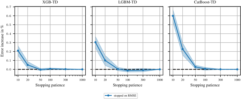
Figure B.2: Effect of stopping patiences on the performance of GBDTs on $\mathcal{B}^{\operatorname{train}}_{\mathrm{reg}}$. We run the TD configurations of XGB, LGBM, and CatBoost with different early stopping patiences (early_stopping_rounds). As in the remainder of the paper, we use RMSE for early stopping and best-epoch selection. The $y$-axis reports the relative increase in the benchmark score relative to stopping on classification error with patience $1000$ (i.e., never stopping early). The shaded areas are approximate 95% confidence intervals, cf. Section C.5.

B.5 Results for AUROC

For classification, there are many different metrics to capture model performance. In the main paper, we use classification error to evaluate models. All TD configurations were tuned for classification error, early stopping and best-epoch selection were performed for classification error, and HPO was performed for classification error. Here, we evaluate models on the area under the ROC curve, also known as AUROC, AUC ROC, or AUC. For the multi-class case, we use the one-vs-rest formulation of AUC, which is faster to evaluate than one-vs-one. Higher AUC values are better and the optimal value is $1$. Since we are interested in the shifted geometric mean error, we use $1-\mathrm{AUC}$ instead.

We compare two settings:

1. A variant of the original setting where early stopping and the selection of the best epoch/iteration is based on accuracy but HPO is performed on $1-\mathrm{AUC}$. (Thanks to using random search, we do not have to re-run the HPO for this.)

2. A setting where we use the cross-entropy loss for stopping and selecting the best epoch/iteration. While it would be possible to stop on AUC directly, this can be significantly slower since AUC is slower to evaluate. We do not perform HPO in this setting since it is expensive to run.

In both settings, we also evaluate RealMLP without label smoothing (no ls). Figure B.4 shows the results optimized for accuracy and Figure B.3 shows the results optimized for cross-entropy. We make a few observations:

• Stopping for cross-entropy generally performs better than stopping for classification error.

• Label smoothing harms RealMLP for AUC, perhaps because the stopping metric does not use label smoothing, or because it encourages near-constant logits in areas where the model is relatively certain.

• Tuned defaults are mostly still better than the library defaults, except for XGBoost on $\mathcal{B}^{\operatorname{test}}_{\mathrm{class}}$.

• RealMLP without label smoothing is still competitive with GBDTs on the meta-test benchmark but does not perform better than GBDTs unlike what we observed for classification error.

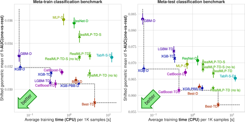
Figure B.3: Benchmark scores on $\mathcal{B}^{\operatorname{train}}_{\mathrm{class}}$ and $\mathcal{B}^{\operatorname{test}}_{\mathrm{class}}$ vs. average training time for AUC, optimized for cross-entropy. BestModel-TD uses RealMLP-TD without label smoothing. The $y$-axis shows the shifted geometric mean ($\operatorname{SGM}_{\varepsilon}$) $1-\mathrm{AUC}$ as explained in Section 2.2. The $x$-axis shows average training times per 1000 samples (measured on $\mathcal{B}^{\operatorname{train}}$ for efficiency reasons), see LABEL:sec:appendix:runtimes. The error bars are approximate 95% confidence intervals for the limit #splits $\to$ $\infty$, see Section C.5.

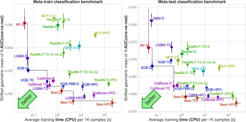
Figure B.4: Benchmark scores on $\mathcal{B}^{\operatorname{train}}_{\mathrm{class}}$ and $\mathcal{B}^{\operatorname{test}}_{\mathrm{class}}$ vs. average training time for AUC. Stopping and best-epoch selection are performed on accuracy, while HPO is performed on AUC. The $y$-axis shows the shifted geometric mean ($\operatorname{SGM}_{\varepsilon}$) $1-\mathrm{AUC}$ as explained in Section 2.2. The $x$-axis shows average training times per 1000 samples (measured on $\mathcal{B}^{\operatorname{train}}$ for efficiency reasons), see LABEL:sec:appendix:runtimes. The error bars are approximate 95% confidence intervals for the limit #splits $\to$ $\infty$, see Section C.5.

B.6 Results Without Missing-Value Datasets

To assess whether the results are influenced by our choices in missing value handling and exclusion, Figure B.5 presents results on all meta-test datasets that originally did not contain missing values. Only six meta-test datasets originally contain missing values: Three from $\mathcal{B}^{\operatorname{test}}_{\mathrm{class}}$ (kick, okcupid-stem, and porto-seguro) and three from $\mathcal{B}^{\operatorname{test}}_{\mathrm{reg}}$ (fps_benchmark, house_prices_nominal, SAT11-HAND-runtime-regression). While RealMLP deteriorates slightly, especially due to the exclusion of fps_benchmark, qualitative takeaways remain similar.

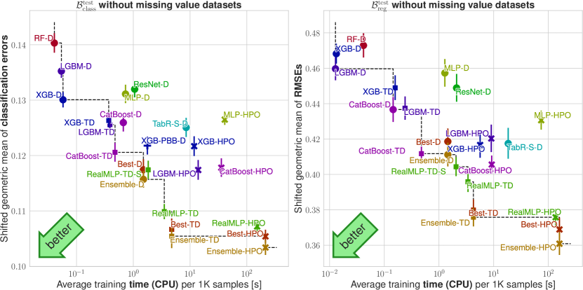
Figure B.5: Benchmark scores on $\mathcal{B}^{\operatorname{test}}_{\mathrm{class}}$ and $\mathcal{B}^{\operatorname{test}}_{\mathrm{reg}}$ without missing value datasets vs. average training time. The $y$-axis shows the shifted geometric mean ($\operatorname{SGM}_{\varepsilon}$) classification error (left) or RMSE (right) as explained in Section 2.2. The $x$-axis shows average training times per 1000 samples (measured on $\mathcal{B}^{\operatorname{train}}$ for efficiency reasons), see LABEL:sec:appendix:runtimes. The error bars are approximate 95% confidence intervals for the limit #splits $\to$ $\infty$, see Section C.5.

B.7 Results for Varying Architecture and Preprocessing

Table B.5 shows the effects of including the preprocessing and architecture of RealMLP within other models. In particular,

• we include robust scaling and smooth clipping (RS+SC) into MLP-D, ResNet-D, and TabR-S-D. By default, these models use a version of the quantile transform (see Section B.2). We observe that it is beneficial on average but not on every benchmark for MLP-D and ResNet-D, while providing notable gains on every benchmark for TabR-S-D.

• we study the benefits of our architectural changes, cf. Figure 1 (c), when applied directly to the setting of MLP-D. To this end, we approximately reproduce MLP-D in our codebase without weight decay (since the optimal value changes when including the NTP) and with marginally different early stopping thresholding logic. We also determine the best default learning rate on the meta-train benchmark, similar to Section A.3. Our reproduction achieves benchmark scores within 1% of the benchmark scores of the MLP-D (RS+SC) version. Adding the PL embeddings from [17] with our default settings sometimes gives good results but is significantly worse on $\mathcal{B}^{\operatorname{test}}_{\mathrm{class}}$, indicating that they need more tuning. In contrast, incorporating the RealMLP architectural changes (including their associated learning rate factors) improves scores on all benchmarks by around 5% or more, although they alone do not match the results of TabR-S-D. However, the non-architectural changes in RealMLP-TD make an even larger difference.

Table B.5: Comparison of preprocessing and architecture for different models. We include variants with robust scaling and smooth clipping (RS+SC), as well as other modified aspects, cf. Section B.7. We report the relative decrease in the shifted geometric mean benchmark scores compared to MLP-D. We also report approximate 95% confidence intervals, cf. Section C.5.

	Error reduction relative to MLP-D in %
Method	meta-train-class	meta-train-reg	meta-test-class	meta-test-reg
MLP-D	-0.0 [-0.0, -0.0]	-0.0 [-0.0, -0.0]	-0.0 [-0.0, -0.0]	-0.0 [-0.0, -0.0]
MLP-D (RS+SC)	1.5 [0.7, 2.4]	-1.6 [-1.9, -1.2]	-0.7 [-1.6, 0.2]	4.3 [3.4, 5.2]
MLP-D (RS+SC, no wd, meta-tuned lr)	2.5 [1.8, 3.3]	-1.0 [-1.5, -0.5]	-1.6 [-2.7, -0.6]	4.3 [3.3, 5.3]
MLP-D (RS+SC, no wd, meta-tuned lr, PL embeddings)	4.6 [4.0, 5.2]	-1.5 [-1.9, -1.0]	-10.9 [-12.3, -9.4]	5.4 [4.0, 6.9]
MLP-D (RS+SC, no wd, meta-tuned lr, RealMLP architecture)	7.7 [6.9, 8.5]	10.4 [9.4, 11.3]	3.2 [2.0, 4.4]	9.6 [8.6, 10.6]
RealMLP-TD-S	12.6 [11.9, 13.2]	13.8 [13.2, 14.4]	9.8 [8.4, 11.2]	13.2 [12.1, 14.3]
RealMLP-TD	16.9 [16.1, 17.6]	22.1 [21.2, 22.9]	15.2 [14.0, 16.5]	14.9 [14.0, 15.8]
TabR-S-D	9.1 [8.2, 10.1]	18.8 [18.3, 19.3]	4.3 [3.0, 5.6]	8.8 [7.8, 9.8]
TabR-S-D (RS+SC)	12.4 [11.6, 13.1]	21.9 [21.1, 22.7]	6.9 [5.6, 8.3]	11.6 [10.4, 12.8]
ResNet-D	-1.9 [-3.0, -0.9]	-6.4 [-7.0, -5.8]	-0.6 [-1.3, 0.1]	0.6 [-0.4, 1.6]
ResNet-D (RS+SC)	2.0 [1.3, 2.8]	-5.9 [-6.6, -5.2]	-1.5 [-2.7, -0.4]	2.3 [1.4, 3.3]

B.8 Comparing HPO Methods

In Figure B.6, we compare two different HPO methods for GBDTs:

• Random search (HPO), as used in the main paper, with 50 steps.

• Tree parzen estimator (HPO-TPE) as implemented in hyperopt [2], with 50 steps. The first 20 of these steps use random search.

While TPE often performs slightly better, the differences in benchmark scores are relatively small.

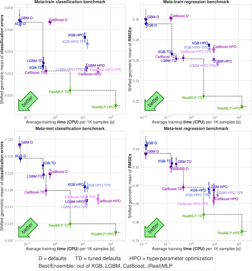
Figure B.6: Benchmark scores of selected methods on $\mathcal{B}^{\operatorname{train}}_{\mathrm{class}}$, $\mathcal{B}^{\operatorname{train}}_{\mathrm{reg}}$, $\mathcal{B}^{\operatorname{test}}_{\mathrm{class}}$, and $\mathcal{B}^{\operatorname{test}}_{\mathrm{reg}}$ vs. average training time. The $y$-axis shows the shifted geometric mean ($\operatorname{SGM}_{\varepsilon}$) classification error (left) or RMSE (right) as explained in Section 2.2. The $x$-axis shows average training times per 1000 samples (measured on $\mathcal{B}^{\operatorname{train}}$ for efficiency reasons), see LABEL:sec:appendix:runtimes. The error bars are approximate 95% confidence intervals for the limit #splits $\to$ $\infty$, see Section C.5.

B.9 More Time-Error Plots

Here, we provide more time-vs-error plots. Figure B.7 shows results for the arithmetic mean error, and Figure B.8 shows results for the arithmetic mean rank, which is also shown in Figure B.9 for the Grinsztajn et al. [19] benchmark. In Figure B.10 we also reproduce the main plots from [19] with added methods.

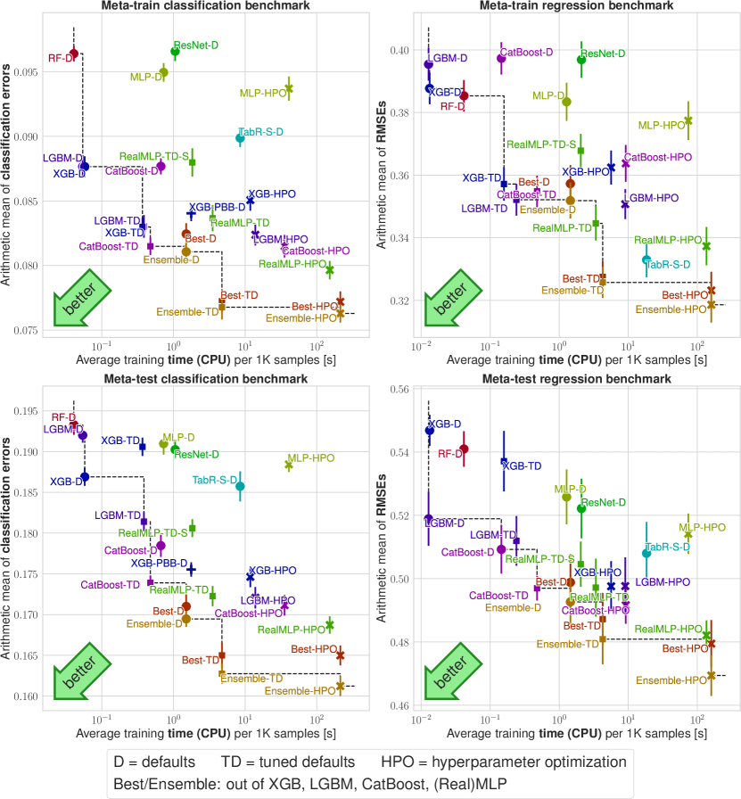
Figure B.7: Benchmark scores (arithmetic mean) vs. average training time. The $y$-axis shows the arithmetic mean classification error (left) or RMSE (right). The $x$-axis shows average training times per 1000 samples (measured on $\mathcal{B}^{\operatorname{train}}$ for efficiency reasons), see LABEL:sec:appendix:runtimes. The error bars are approximate 95% confidence intervals for the limit #splits $\to$ $\infty$, see Section C.5.

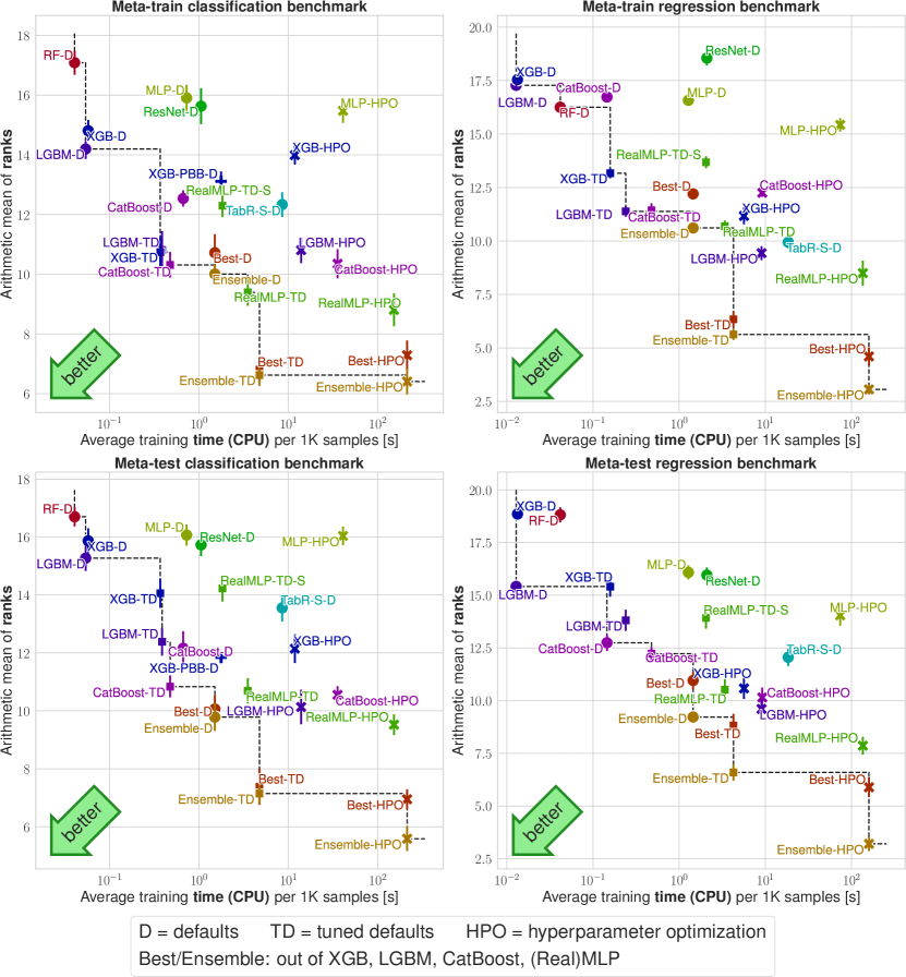
Figure B.8: Benchmark scores (ranks) vs. average training time. The $y$-axis shows the arithmetic mean rank, averaged over all splits and datasets. The $x$-axis shows average training times per 1000 samples (measured on $\mathcal{B}^{\operatorname{train}}$ for efficiency reasons), see LABEL:sec:appendix:runtimes. The error bars are approximate 95% confidence intervals for the limit #splits $\to$ $\infty$, see Section C.5.

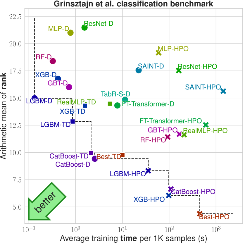
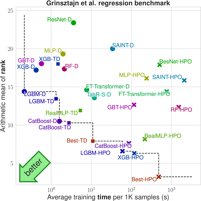
Figure B.9: Results on the benchmarks of Grinsztajn et al. [19]. The $y$-axis shows the arithmetic mean rank of each model. The $x$-axis shows average training times per 1000 samples, see LABEL:sec:appendix:runtimes.

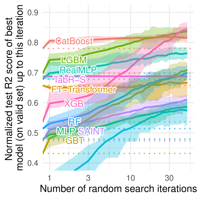
Figure B.10: Results on the benchmarks of Grinsztajn et al. [19], for classification (left) and regression (right). The plot is similar to the one in the main part of [19], with our algorithms added. The $y$-axis shows the result of the best (on val, but evaluated on test) hyperparameter combination up to n steps of random step ($x$-axis). As in the original paper, we normalize each score between the max and the 10% quantile (classification) or 50% (regression), and truncate scores below 0 for regression.

B.10 Critical Difference Diagrams

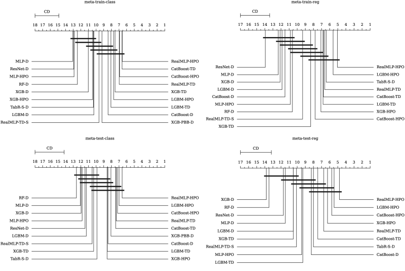
Figure B.11: Critical difference diagrams on the meta-train and meta-test benchmarks. The plots show the average rank of methods on each benchmark. Horizontal bars indicate groups of algorithms that are not statistically significantly different at a 95% confidence level according to a Friedman test and post-hoc Nemenyi test implemented in autorank [23].

Figure B.11 analyzes the external validity of differences in average ranks between methods, i.e., whether they will generalize to new datasets from a distribution. While establishing external validity requires a large number of datasets, our benchmarks consistently show the improvements of RealMLP-TD over MLP-D to be externally valid.

B.11 Win-rate Plots

For pairs of methods, we analyze the percentage of (dataset, split) combinations on which the first method has a lower error than the second method. We plot these win-rates in marix plots: Figure B.12 shows the results on $\mathcal{B}^{\operatorname{train}}_{\mathrm{class}}$, Figure B.13 shows the results on $\mathcal{B}^{\operatorname{test}}_{\mathrm{class}}$, Figure B.14 shows the results on $\mathcal{B}^{\operatorname{train}}_{\mathrm{reg}}$, and Figure B.15 shows the results on $\mathcal{B}^{\operatorname{test}}_{\mathrm{reg}}$.

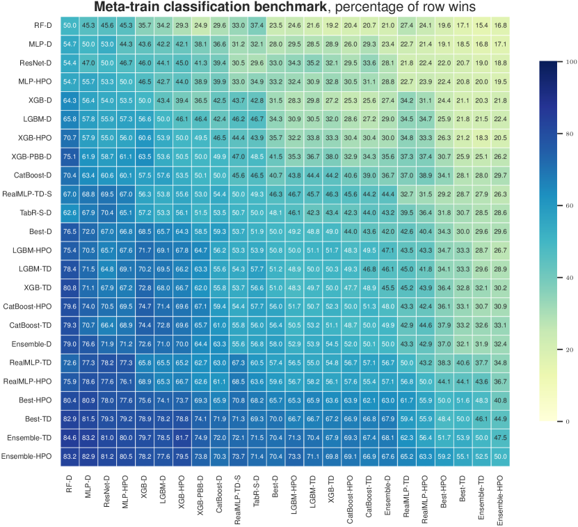
Figure B.12: Percentages of wins of row algorithms vs column algorithms on $\mathcal{B}^{\operatorname{train}}_{\mathrm{class}}$. Wins are averaged over all datasets and splits. Ties count as half-wins. Methods are sorted by average winrate (i.e., the average of the values in the row). When averaging, we use dataset-dependent weighting as explained in Section C.3.1.

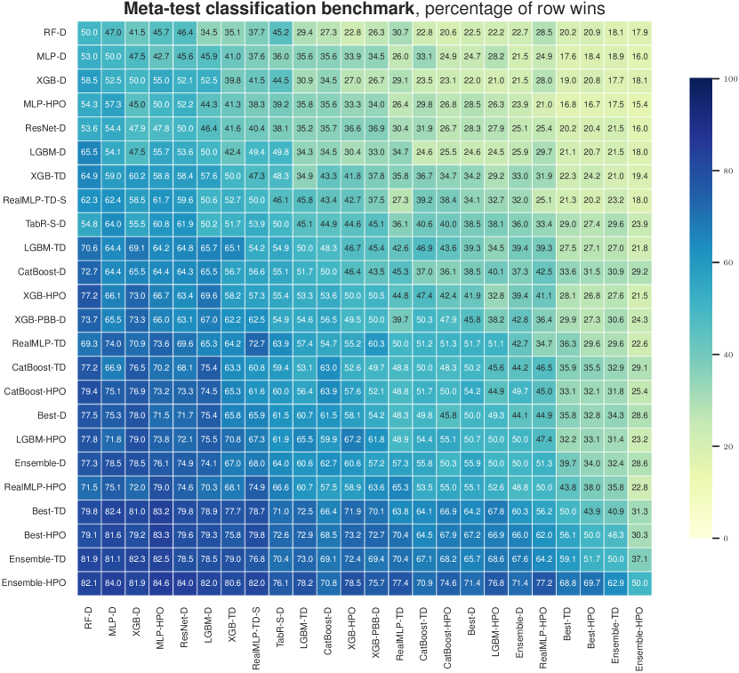
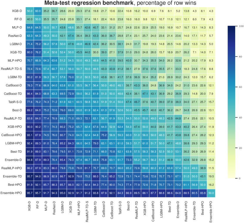
Figure B.13: Percentages of wins of row algorithms vs column algorithms on $\mathcal{B}^{\operatorname{test}}_{\mathrm{class}}$. Wins are averaged over all datasets and splits. Ties count as half-wins. Methods are sorted by average winrate (i.e., the average of the values in the row).

Figure B.14: Percentages of wins of row algorithms vs column algorithms on $\mathcal{B}^{\operatorname{train}}_{\mathrm{reg}}$. Wins are averaged over all datasets and splits. Ties count as half-wins. Methods are sorted by average winrate (i.e., the average of the values in the row). When averaging, we use dataset-dependent weighting as explained in Section C.3.1.

Figure B.15: Percentages of wins of row algorithms vs column algorithms on $\mathcal{B}^{\operatorname{test}}_{\mathrm{reg}}$. Wins are averaged over all datasets and splits. Ties count as half-wins. Methods are sorted by average winrate (i.e., the average of the values in the row).

Appendix C Benchmark Details

C.1 Default Configurations

The parameters for RealMLP-TD and RealMLP-TD-S have already been given in Table A.1. Table C.1 shows the hyperparameters of LGBM-TD and LGBM-D. Table C.2 shows the hyperparameters of XGB-TD and XGB-D. Table C.3 shows the hyperparameters of CatBoost-TD and CatBoost-D. The parameters for LGBM-D, XGB-D, and CatBoost-D have been taken from the respective libraries at the time of writing and are given here for completeness. The parameters for MLP-D are given in Table C.4 and the parameters for ResNet-D are given in Table C.5. By “RTDL quantile transform”, we refer to the version adding noise before fitting the quantile transform. The parameters for TabR-S-D are given in Table C.6. On the dionis dataset, we activate context freeze for TabR-S-D after four epochs, since training can take up to 30 GPU-hours even with context freeze.

For XGB-PBB-D, we use the default parameters from [50], with the following modifications: We use hist gradient boosting since it is the new default in XGBoost 2.0. Moreover, since we have high-cardinality categories, we limit one-hot encoding to categories with less than 20 distinct values (not counting missing values), and use XGBoost’s native categorical feature handling for the remaining categorical features.

Table C.1: Hyperparameters for LGBM-TD and LGBM-D. Italic hyperparameters have not been tuned.

Hyperparameter	LGBM-TD		LGBM-D
	classif.	reg.
num_leaves	50	100	31
learning_rate	0.04	0.05	0.1
subsample	0.75	0.7	1.0
colsample_bytree	1.0	1.0	1.0
min_data_in_leaf	40	3	20
min_sum_hessian_in_leaf	1e-7	1e-7	1e-3
n_estimators	1000	1000	100
bagging_freq	1	1	1
max_bin	255	255	255
early_stopping_rounds	300	300	1000

Table C.2: Hyperparameters for XGB-TD and XGB-D. Italic hyperparameters have not been tuned for XGB-TD.

Hyperparameter	XGB-TD		XGB-D
	classif.	reg.
max_depth	6	9	6
learning_rate	0.08	0.05	0.3
subsample	0.65	0.7	1.0
colsample_bytree	1.0	1.0	1.0
colsample_bylevel	0.9	1.0	1.0
min_child_weight	5e-6	2.0	1.0
lambda	0.0	0.0	1.0
tree_method	hist	hist	hist
n_estimators	1000	1000	100
max_bin	256	256	256
early_stopping_rounds	300	300	1000

Table C.3: Hyperparameters for CatBoost-TD and CatBoost-D. Italic hyperparameters have not been tuned for CatBoost-TD.

Hyperparameter	CatBoost-TD		CatBoost-D
	classif.	reg.
boosting_type	Plain	Plain	Plain
bootstrap_type	Bernoulli	Bernoulli	Bayesian
max_depth	7	9	6
learning_rate	0.08	0.09	automatic
subsample	0.9	0.9	—
bagging_temperature	—	—	1.0
l2_leaf_reg	1e-5	1e-5	3.0
random_strength	0.8	0.0	1.0
one_hot_max_size	15	20	2
leaf_estimation_iterations	1	20	None
n_estimators	1000	1000	1000
max_bin	254	254	256
od_wait	300	300	None
od_type	Iter	Iter	Iter

Table C.4: Hyperparameters for MLP-D, adapted from [43].

Hyperparameter	Space
lr scheduler	None
n_layers	3
d_layers	[128, 256, 128]
Dropout prob.	0.1
lr	1e-3
Optimizer	AdamW
d_embedding	8
batch_size	128
max_epochs	1000
early stopping patience	20
Preprocessing	RTDL quantile transform
Activation function	ReLU
Initialization	PyTorch default
Weight decay	0.01

Table C.5: Hyperparameters for ResNet-D, adapted from [43].

Hyperparameter	Space
lr scheduler	None
Activation	ReLU
Normalization	BatchNorm
n_layers	2
d_layers	[128, 128]
d_hidden_factor	2
hidden_dropout	0.25
residual_dropout	0.1
lr	1e-3
weight_decay	0.01
Optimizer	AdamW
d_embedding	8
batch_size	128
max_epochs	1000
early stopping patience	20
Preprocessing	RTDL quantile transform

Table C.6: Hyperparameters for TabR-S-D, taken from [18].

Hyperparameter	Space
num_embeddings	None
d_main	265
context_dropout	0.38920071545944357
d_multiplier	2.0
encoder_n_blocks	0
predictor_n_blocks	1
mixer_normalization	auto
dropout0	0.38852797479169876
dropout1	0.0
normalization	LayerNorm
activation	ReLU
batch_size	auto
patience	16
n_epochs	100,000
context_size	96
optimizer	AdamW
lr	0.0003121273641315169
weight_decay	1.2260352006404615e-06
Preprocessing	RTDL quantile transform

C.2 Hyperparameter Optimization

For LGBM-HPO, XGB-HPO, and CatBoost-HPO, we run 50 steps of random search using the search spaces presented in Table C.7, C.8, and C.9, respectively. These search spaces are adapted from the literature, using n_estimators=1000 in each case.

For RealMLP-HPO, we run 50 steps of random search. We provide a custom search space specified in Table C.10. For MLP-HPO, we also run 50 steps of random search with the search space in Table C.11, adapted from [16].

Table C.7: Hyperparameter seach space for LGBM-HPO, adapted from [51] with 1000 estimators instead of 5000.

Hyperparameter	Space
n_estimators	1000
bagging_freq	1
early_stopping_rounds	300
num_leaves	LogUniformInt[1, $e^{7}$]
learning_rate	LogUniform[$e^{-7}$, 1]
subsample	Uniform[0.5, 1]
feature_fraction	Uniform[0.5, 1]
min_data_in_leaf	LogUniformInt[1, $e^{6}$]
min_sum_hessian_in_leaf	LogUniform[$e^{-16}$, $e^{5}$]
lambda_l1	Random$\{$0, LogUniform[$e^{-16}$, $e^{2}$]$\}$
lambda_l2	Random$\{$0, LogUniform[$e^{-16}$, $e^{2}$]$\}$

Table C.8: Hyperparameter search space for XGB-HPO, adapted from [19]. We use the hist method, which is the new default in XGBoost 2.0 and supports native handling of categorical values, while the old auto method selection is not available in XGBoost 2.0. We also increase early_stopping_rounds to 300.

Hyperparameter	Space
tree_method	hist
n_estimators	1000
early_stopping_rounds	300
max_depth	UniformInt[1, 11]
learning_rate	LogUniform[1e-5, 0.7]
subsample	Uniform[0.5, 1]
colsample_bytree	Uniform[0.5, 1]
colsample_bylevel	Uniform[0.5, 1]
min_child_weight	LogUniformInt[1, 100]
alpha	LogUniform[1e-8, 1e-2]
lambda	LogUniform[1, 4]
gamma	LogUniform[1e-8, 7.0]

Table C.9: Hyperparameter search space for CatBoost-HPO, adapted from [57], who did not specify the number of estimators.

Hyperparameter	Space
boosting_type	Plain
bootstrap_type	Bayesian
n_estimators	1000
max_depth	6
od_wait	300
od_type	Iter
learning_rate	LogUniform[$e^{-5}$, 1]
bagging_temperature	Uniform[0, 1]
l2_leaf_reg	LogUniform[0, 10]
random_strength	UniformInt[1, 20]
one_hot_max_size	UniformInt[0, 25]
leaf_estimation_iterations	UniformInt[1, 20]

Table C.10: Hyperparameter search space for RealMLP-HPO. The remaining hyperparameters are set as in RealMLP-TD.

Hyperparameter	classif.	reg.
Num. embedding type	Choice([None, PBLD, PL, PLR])	same
Use scaling layer	Choice([True, False], p=[0.6, 0.4])	same
Learning rate	LogUniform([2e-2, 3e-1])	same
Dropout prob.	Choice([0.0, 0.15, 0.3], p=[0.3, 0.5, 0.2])	same
Activation fct.	Choice([ReLU, SELU, Mish])	same
Hidden layer sizes	Choice([[256, 256, 256], [64, 64, 64, 64, 64], [512]], p=[0.6, 0.2, 0.2])	same
Weight decay	Choice([0.0, 2e-2])	same
$\boldsymbol{w}^{(1,i)}_{\text{emb}}$ init std.	LogUniform([0.05, 0.5])
Label smoothing $\varepsilon$	Choice([0.0, 0.1], p=[0.3, 0.7])	no label smoothing

Table C.11: Hyperparameter search space for MLP-HPO, adapted from [16]. We reduced the embedding dimension upper bound, the maximum number of epochs, and the number of layers to have a more acceptable runtime on the meta-test benchmarks. We also used a minimum batch size of 256. As in the original paper, the size of the first and the last layers are tuned and set separately, while the size for “in-between” layers is the same for all of them.

Hyperparameter	Space
	#samples$\leq$100,000	#samples$>$100,000
n_layers	UniformInt[1, 8]	UniformInt[1, 11]
d	UniformInt[64, 512]	UniformInt[64, 1024]
d_hidden_factor	UniformInt[1, 4]
hidden_dropout	Uniform[0, 0.5]
residual_dropout	Choice(0, Uniform[0, 0.5])
lr	LogUniform[1e-5, 1e-2]
weight decay	Choice(0, LogUniform[1e-6, 1e-3])
d_embedding	UniformInt[8, 31]
batch_size	256 if train_size < 30K
	else 512 if train_size < 100K else 1024
lr_scheduler	None
Optimizer	AdamW
max #epochs	400
early stopping patience	16
Preprocessing	RTDL quantile transform

C.3 Dataset Selection and Preprocessing

C.3.1 Meta-train Benchmarks

For the meta-train benchmarks, we adapt code from [60] to collect all datasets from the UCI repository that follow certain criteria:

• Between 2,500 and 50,000 samples.

• Number of features at most 1,000.

• Labeled as classification or regression task.

• Description made it straightforward to convert the original dataset into a numeric .csv format.

• Uploaded before 2019-05-08.

We remove rows with missing values and keep only those datasets that still have at least 2,500 samples. Some datasets are labeled both as regression and classification datasets, in which case we use them for both. We standardize the targets for regression datasets, such that a constant predictor can achieve an RMSE of 1. Some datasets contain different versions (e.g., different target columns), in which case we use all of them. To avoid biasing the results towards one dataset, we compute benchmark scores using weights proportional to $1/\#\text{versions}$. In total, we obtain 71 classification datasets (including versions) out of 46 original datasets, and 47 regression datasets (including versions) out of 26 original datasets. Tables C.12 and C.13 summarize key characteristics of these datasets. We count datasets with the same prefix (before the first underscore) as being versions of the same dataset for weighting, except for the two “facebook” datasets in $\mathcal{B}^{\operatorname{train}}_{\mathrm{reg}}$, which we count as distinct. For regression, we standardize the targets to have mean zero and variance 1.

During earlier development of the MLP, the meta-train benchmark used to include an epileptic seizure recognition dataset, which has since been removed from the UCI repository, hence we do not report results on it.

Table C.12: Datasets in the meta-train classification benchmark.

Name	#samples	#num. features	#cat. features	largest #categories	#classes
abalone	4177	8	0		3
adult	45222	7	7	41	2
anuran_calls_families	7127	22	0		3
anuran_calls_genus	6073	22	0		5
anuran_calls_species	5696	22	0		7
avila	20867	10	0		12
bank_marketing	41579	12	5	11	2
bank_marketing_additional	39457	19	3	11	2
chess	3196	1	31	3	2
chess_krvk	28056	3	3	8	18
crowd_sourced_mapping	10494	28	0		4
default_credit_card	30000	23	1	2	2
eeg_eye_state	14980	14	0		2
electrical_grid_stability_simulated	10000	12	0		2
facebook_live_sellers_thailand_status	6622	9	0		2
firm_teacher_clave	10800	0	16	2	4
first_order_theorem_proving	6118	51	0		2
gas_sensor_drift_class	13910	128	0		6
gesture_phase_segmentation_raw	9900	19	0		5
gesture_phase_segmentation_va3	9873	32	0		5
htru2	17898	8	0		2
human_activity_smartphone	10299	561	0		6
indoor_loc_building	21048	470	50	2	3
indoor_loc_relative	21048	470	50	2	3
insurance_benchmark	9822	80	4	5	2
landsat_satimage	6435	36	0		6
letter_recognition	20000	16	0		26
madelon	2600	500	0		2
magic_gamma_telescope	19020	10	0		2
mushroom	8124	0	21	12	2
musk	6598	166	0		2
nomao	34465	118	2	2	2
nursery	12960	7	1	2	4
occupancy_detection	20560	7	0		2
online_shoppers_attention	12330	16	2	3	2
optical_recognition_handwritten_digits	5620	59	3	2	10
ozone_level_1hr	1848	72	0		2
ozone_level_8hr	1847	72	0		2
page_blocks	5473	10	0		5
pen_recognition_handwritten_characters	10992	16	0		10
phishing	11055	8	22	2	2
polish_companies_bankruptcy_1year	7027	64	0		2
polish_companies_bankruptcy_2year	10173	64	0		2
polish_companies_bankruptcy_3year	10503	64	0		2
polish_companies_bankruptcy_4year	9792	64	0		2
polish_companies_bankruptcy_5year	5910	64	0		2
seismic_bumps	2584	12	3	2	2
skill_craft	3338	18	0		7
smartphone_human_activity	5744	561	0		6
smartphone_human_activity_postural	10411	561	0		6
spambase	4601	57	0		2
superconductivity_class	21263	81	0		2
thyroid_all_bp	3621	6	17	5	2
thyroid_all_hyper	3621	6	17	5	2
thyroid_all_hypo	3621	6	17	5	3
thyroid_all_rep	3621	6	17	5	2
thyroid_ann	7200	6	11	3	3
thyroid_dis	3621	6	17	5	2
thyroid_hypo	2700	7	14	3	2
thyroid_sick	3621	6	17	5	2
thyroid_sick_eu	3163	8	18	2	2
turkiye_student_evaluation	5820	32	0		3
wall_follow_robot_2	5456	2	0		4
wall_follow_robot_24	5456	24	0		4
wall_follow_robot_4	5456	4	0		4
waveform	5000	21	0		3
waveform_noise	5000	40	0		3
wilt	4839	5	0		2
wine_quality_all	6497	11	1	2	7
wine_quality_type	6497	11	0		2
wine_quality_white	4898	11	0		7

Table C.13: Datasets in the meta-train regression benchmark.

Name	#samples	#num. features	#cat. features	largest #categories
air_quality_bc	8991	10	0
air_quality_co2	7674	10	0
air_quality_no2	7715	10	0
air_quality_nox	7718	10	0
appliances_energy	19735	29	0
bejing_pm25	41757	12	0
bike_sharing_casual	17379	9	3	2
bike_sharing_total	17379	9	3	2
carbon_nanotubes_u	10721	5	0
carbon_nanotubes_v	10721	5	0
carbon_nanotubes_w	10721	5	0
chess_krvk	28056	3	3	8
cycle_power_plant	9568	4	0
electrical_grid_stability_simulated	10000	12	0
facebook_comment_volume	40949	38	2	7
facebook_live_sellers_thailand_shares	7050	9	0
five_cities_beijing_pm25	19062	14	0
five_cities_chengdu_pm25	21074	14	0
five_cities_guangzhou_pm25	20074	14	0
five_cities_shanghai_pm25	21436	14	0
five_cities_shenyang_pm25	19038	14	0
gas_sensor_drift_class	13910	128	0
gas_sensor_drift_conc	13910	128	0
indoor_loc_alt	21048	470	50	2
indoor_loc_lat	21048	470	50	2
indoor_loc_long	21048	470	50	2
insurance_benchmark	9822	80	4	5
metro_interstate_traffic_volume_long	48204	6	2	38
metro_interstate_traffic_volume_short	48204	6	2	11
naval_propulsion_comp	11934	14	0
naval_propulsion_turb	11934	14	0
nursery	12960	7	1	2
online_news_popularity	39644	44	3	7
parking_birmingham	35717	5	0
parkinson_motor	5875	18	1	2
parkinson_total	5875	18	1	2
protein_tertiary_structure	45730	9	0
skill_craft	3338	18	0
sml2010_dining	4137	17	0
sml2010_room	4137	17	0
superconductivity	21263	81	0
travel_review_ratings	5456	23	0
wall_follow_robot_2	5456	2	0
wall_follow_robot_24	5456	24	0
wall_follow_robot_4	5456	4	0
wine_quality_all	6497	11	1	2
wine_quality_white	4898	11	0

C.3.2 Meta-test Benchmarks

The meta-test benchmarks consist of datasets from the AutoML Benchmark [14] and additional regression datasets from the OpenML-CTR23 benchmark [13], obtained from OpenML [64].

We make the following modifications:

• We use brazilian_houses from OpenML-CTR23 and exclude Brazilian_houses from the AutoML regression benchmark, since the latter contains three additional features that should not be used for predicting the target.

• We use another version of the sarcos dataset where the original test set is not included, since the original test set consists of duplicates of training samples.

• We excluded the following datasets because versions of them were already contained in the meta-training set:

  • For classification: kr-vs-kp, wilt, ozone-level-8hr, first-order-theorem-proving, GesturePhaseSegmentationProcessed, PhishingWebsites, wine-quality-white, nomao, bank-marketing, adult

  • For regression: wine_quality, abalone, OnlineNewsPopularity, Brazilian_houses, physicochemical_protein, naval_propulsion_plant, superconductivity, white_wine, red_wine, grid_stability

We preprocess the datasets as follows:

• We remove rows with missing continuous values

• We subsample large datasets to contain at most 500,000 samples. Since the dionis dataset was particularly slow to train with GBDT models due to its 355 classes, we subsampled it to 100,000 samples.

• We standardize the targets for regression datasets, such that a constant predictor can achieve an RMSE of 1.

• We encode missing categorical values as a separate category.

• For regression, we standardize the targets to have mean zero and variance 1.

After preprocessing, we

• exclude datasets with less than 1,000 samples, these were

  • for classification: albert, APSFailure, arcene, Australian, blood-transfusion-service-center, eucalyptus, KDDCup09_appetency, KDDCup09-Upselling, micro-mass, vehicle

  • for regression: boston, cars, colleges, energy_efficiency, forest_fires, Moneyball, QSAR_fish_toxicity, sensory, student_performance_por, tecator, us_crime

• exclude datasets that have more than 10,000 features after one-hot encoding. These were Amazon_employee_access, Click_prediction_small, and sf-police-incidents (all classification).

Table C.14: Datasets in the meta-test classification benchmark.

Name	#samples	#num. features	#cat. features	largest #categories	#classes	OpenML task ID
Bioresponse	3751	1776	0		2	359967
Diabetes130US	101766	13	36	789	3	211986
Fashion-MNIST	70000	784	0		10	359976
Higgs	500000	28	0		2	360114
Internet-Advertisements	3279	3	1555	2	2	359966
KDDCup99	500000	32	9	65	21	360112
MiniBooNE	130064	50	0		2	359990
Satellite	5100	36	0		2	359975
ada	4147	48	0		2	190411
airlines	500000	3	4	293	2	189354
amazon-commerce-reviews	1500	10000	0		50	10090
car	1728	0	6	4	4	359960
christine	5418	1599	37	2	2	359973
churn	5000	16	4	10	2	359968
cmc	1473	2	7	4	3	359959
cnae-9	1080	856	0		9	359957
connect-4	67557	0	42	3	3	359977
covertype	500000	10	44	2	7	7593
credit-g	1000	7	13	10	2	168757
dilbert	10000	2000	0		5	168909
dionis	100000	60	0		355	189355
dna	3186	0	180	2	3	359964
fabert	8237	800	0		7	168910
gina	3153	970	0		2	189922
guillermo	20000	4296	0		2	359988
helena	65196	27	0		100	359984
jannis	83733	54	0		4	211979
jasmine	2984	8	136	2	2	168911
jungle_chess_2pcs_raw_endgame_complete	44819	6	0		3	359981
kc1	2109	21	0		2	359962
kick	72600	14	18	1054	2	359991
madeline	3140	259	0		2	190392
mfeat-factors	2000	216	0		10	359961
numerai28.6	96320	21	0		2	167120
okcupid-stem	50788	2	17	7019	3	359993
pc4	1458	37	0		2	359958
philippine	5832	308	0		2	190410
phoneme	5404	5	0		2	168350
porto-seguro	453046	26	31	102	2	360113
qsar-biodeg	1055	41	0		2	359956
riccardo	20000	4296	0		2	359989
robert	10000	7200	0		10	359986
segment	2310	16	0		7	359963
shuttle	58000	9	0		7	359987
steel-plates-fault	1941	27	0		7	168784
sylvine	5124	20	0		2	359972
volkert	58310	180	0		10	359985
yeast	1484	8	0		10	2073

Table C.15: Datasets in the meta-test regression benchmark.

Name	#samples	#num. features	#cat. features	largest #categories	OpenML task ID
Airlines_DepDelay_10M	500000	6	3	359	359929
Allstate_Claims_Severity	188318	14	116	326	233212
Buzzinsocialmedia_Twitter	500000	77	0		233213
MIP-2016-regression	1090	143	1	5	360945
Mercedes_Benz_Greener_Manufacturing	4209	368	8	47	233215
QSAR-TID-10980	5766	1024	0		360933
QSAR-TID-11	5742	1024	0		360932
SAT11-HAND-runtime-regression	1725	115	1	15	359948
Santander_transaction_value	4459	4991	0		233214
Yolanda	400000	100	0		317614
airfoil_self_noise	1503	5	0		361235
auction_verification	2043	5	2	6	361236
black_friday	166821	5	4	7	359937
brazilian_houses	10692	5	4	35	361267
california_housing	20640	8	0		361255
concrete_compressive_strength	1030	8	0		361237
cps88wages	28155	2	4	4	361261
cpu_activity	8192	21	0		361256
diamonds	53940	6	3	8	361257
elevators	16599	18	0		359936
fifa	19178	27	1	163	361272
fps_benchmark	2592	29	14	24	361268
geographical_origin_of_music	1059	116	0		361243
health_insurance	22272	4	7	6	361269
house_16H	22784	16	0		359952
house_prices_nominal	1121	36	43	25	359951
house_sales	21613	20	1	70	359949
kin8nm	8192	8	0		361258
kings_county	21613	17	4	70	361266
miami_housing	13932	15	0		361260
nyc-taxi-green-dec-2016	500000	9	9	259	359943
pol	15000	48	0		359946
pumadyn32nh	8192	32	0		361259
quake	2178	3	0		359930
sarcos	44484	21	0		361011
socmob	1156	1	4	17	361264
solar_flare	1066	2	8	6	361244
space_ga	3107	6	0		361623
topo_2_1	8885	266	0		359939
video_transcoding	68784	16	2	4	361252
wave_energy	72000	48	0		361253
yprop_4_1	8885	251	0		359940

C.4 Grinsztajn et al. benchmark

The datasets are taken from the benchmarks described in [19]. When a dataset is used both in benchmarks with and without categorical features, we use the version with categorical features. We preprocess the datasets following the same steps as in [19]:

• For neural networks, we quantile-transform the features to have a Gaussian distribution. For TabR [18], we use the modified quantile transform from the TabR paper. For RealMLP, we use the preprocessing described in Section 3, namely robust scaling and smooth clipping.

• For neural networks, we add as a hyperparameter the possibility to normalize the target variable for the model fit and transform it back for evaluation (via scikit-learn’s TransformedTargetRegressor and StandardScaler, which differs from the QuantileTransformer from the original paper, as we found it to work better). The same standardization is also applied to all default-parameter versions of neural networks.

• For models that do not handle categorical variables natively, we encode categorical features using OneHotEncoder from scikit-learn.

• Train size is restricted to 10,000 samples and test and validation size to 50,000 samples.

Note that the datasets from the original benchmark are already slightly preprocessed, e.g., heavy-tailed targets are standardized and missing values are removed. More details can be found in the original paper.

Results normalization

For Figure 3, as in the original paper, we normalize the R2 or accuracy score for each dataset before averaging them. We use an affine normalization between 0 and 1, 1 corresponding to the score of the best model for each dataset, and 0 corresponding to the score of the worst model (for classification) and the 10th percentile of the scores (for regression). We use slightly different percentiles compared to the original paper as we normalize across the scores of the tuned and default models, and not all steps of the random search, which reduces the number of outliers. Other aggregation metrics are shown in Section B.9.

Other details

We rerun classification results for neural networks compared to the original results to early stop on accuracy rather than on cross-entropy, to make results more comparable with the rest of this paper.

C.5 Confidence Intervals

Here, we specify how our confidence intervals are computed. Let $X_{ij}$ denote the score (error/rank) of a method on dataset $i$ and split $j$, with $i\in\{1,\ldots,n\}$ and $j\in\{1,\ldots,m\}$. Then, the benchmark score $\mathcal{S}$ can be written as +rCl+x* S= g(∑_i=1^n wim ∑_j=1^m f(X_ij)), where $f=g=\operatorname{id}$ for the arithmetic mean. For the shifted geometric mean, we instead have $g=\exp$ and $f(x)=\log(x+\varepsilon)$, $\varepsilon=0.01$. We interpret the benchmark datasets as fixed, but the splits as random. For each dataset $i$, $X_{i1},\ldots,X_{im}$ are i.i.d. random variables. We first take the dataset averages +rCl+x* Z_j ≔∑_i=1^n w_i f(X_ij) . The random variables $X_{1j},\ldots,X_{nj}$ are independent but not identically distributed. Still, for lack of a better option, we assume that the $Z_{j}$ are normally distributed with unknown mean and variance. We know that the $Z_{j}$ are i.i.d., hence we use the confidence intervals from the Student’s $t$-distribution for normally distributed random variables with unknown mean and variance. This gives us a confidence interval $[a,b]$ for $\frac{1}{m}\sum_{j=1}^{m}Z_{j}$. Since $g$ is increasing, we hence obtain a confidence interval $[g(a),g(b)]$ for $\mathcal{S}=g\left(\frac{1}{m}\sum_{j=1}^{m}Z_{j}\right)$.

Comparison of two methods

We often compute the error increase in % in the benchmark score of method A compared to method B with the shifted geometric mean, given by +rCl+x* 100 ⋅(S(A)S(B) - 1) . Here, we leverage that the shifted geometric mean uses $g=\exp$ to write +rCl+x*

References

- Arik and Pfister [2021] Sercan O. Arik and Tomas Pfister. TabNet: Attentive interpretable tabular learning. In AAAI Conference on Artificial Intelligence, 2021.
- Bergstra et al. [2013] James Bergstra, Daniel Yamins, and David Cox. Making a science of model search: Hyperparameter optimization in hundreds of dimensions for vision architectures. In International Conference on Machine Learning, 2013.
- Borisov et al. [2022] Vadim Borisov, Tobias Leemann, Kathrin Seßler, Johannes Haug, Martin Pawelczyk, and Gjergji Kasneci. Deep neural networks and tabular data: A survey. IEEE Transactions on Neural Networks and Learning Systems, 2022.
- Brazdil et al. [2008] Pavel Brazdil, Christophe Giraud Carrier, Carlos Soares, and Ricardo Vilalta. Metalearning: Applications to Data Mining. Springer Science & Business Media, 2008.
- Breiman [2001] Leo Breiman. Random forests. Machine learning, 45:5–32, 2001.
- Caruana et al. [2004] Rich Caruana, Alexandru Niculescu-Mizil, Geoff Crew, and Alex Ksikes. Ensemble selection from libraries of models. In International Conference on Machine Learning, 2004.
- Caruana et al. [2006] Rich Caruana, Art Munson, and Alexandru Niculescu-Mizil. Getting the most out of ensemble selection. In International Conference on Data Mining, pages 828–833. IEEE, 2006.
- Chen et al. [2023a] Jintai Chen, Jiahuan Yan, Danny Ziyi Chen, and Jian Wu. ExcelFormer: A neural network surpassing GBDTs on tabular data. arXiv:2301.02819, 2023a.
- Chen et al. [2023b] Kuan-Yu Chen, Ping-Han Chiang, Hsin-Rung Chou, Ting-Wei Chen, and Tien-Hao Chang. Trompt: Towards a better deep neural network for tabular data. In International Conference on Machine Learning, 2023b.
- Chen and Guestrin [2016] Tianqi Chen and Carlos Guestrin. XGBoost: A scalable tree boosting system. In International Conference on Knowledge Discovery and Data Mining, 2016.
- Erickson et al. [2020] Nick Erickson, Jonas Mueller, Alexander Shirkov, Hang Zhang, Pedro Larroy, Mu Li, and Alexander Smola. AutoGluon-Tabular: Robust and accurate AutoML for structured data. In 7th ICML Workshop on Automated Machine Learning, 2020.
- Feurer et al. [2022] Matthias Feurer, Katharina Eggensperger, Stefan Falkner, Marius Lindauer, and Frank Hutter. Auto-sklearn 2.0: Hands-free automl via meta-learning. The Journal of Machine Learning Research, 23(261), 2022.
- Fischer et al. [2023] Sebastian Felix Fischer, Matthias Feurer, and Bernd Bischl. OpenML-CTR23–A curated tabular regression benchmarking suite. In AutoML Conference 2023 (Workshop), 2023.
- Gijsbers et al. [2022] Pieter Gijsbers, Marcos LP Bueno, Stefan Coors, Erin LeDell, Sébastien Poirier, Janek Thomas, Bernd Bischl, and Joaquin Vanschoren. AMLB: An AutoML benchmark. arXiv:2207.12560, 2022.
- Gneiting and Raftery [2007] Tilmann Gneiting and Adrian E Raftery. Strictly proper scoring rules, prediction, and estimation. Journal of the American Statistical Association, 102(477):359–378, 2007.
- Gorishniy et al. [2021] Yury Gorishniy, Ivan Rubachev, Valentin Khrulkov, and Artem Babenko. Revisiting deep learning models for tabular data. Neural Information Processing Systems, 2021.
- Gorishniy et al. [2022] Yury Gorishniy, Ivan Rubachev, and Artem Babenko. On embeddings for numerical features in tabular deep learning. Neural Information Processing Systems, 2022.
- Gorishniy et al. [2023] Yury Gorishniy, Ivan Rubachev, Nikolay Kartashev, Daniil Shlenskii, Akim Kotelnikov, and Artem Babenko. TabR: Tabular deep learning meets nearest neighbors in 2023. arXiv:2307.14338, 2023.
- Grinsztajn et al. [2022] Léo Grinsztajn, Edouard Oyallon, and Gaël Varoquaux. Why do tree-based models still outperform deep learning on typical tabular data? Neural Information Processing Systems, 2022.
- Guo and Berkhahn [2016] Cheng Guo and Felix Berkhahn. Entity embeddings of categorical variables. arXiv:1604.06737, 2016.
- Hafner et al. [2023] Danijar Hafner, Jurgis Pasukonis, Jimmy Ba, and Timothy Lillicrap. Mastering diverse domains through world models. arXiv:2301.04104, 2023.
- He et al. [2015] Kaiming He, Xiangyu Zhang, Shaoqing Ren, and Jian Sun. Delving deep into rectifiers: Surpassing human-level performance on imagenet classification. In IEEE International Conference on Computer Vision, pages 1026–1034, 2015.
- Herbold [2020] Steffen Herbold. Autorank: A Python package for automated ranking of classifiers. Journal of Open Source Software, 5(48):2173, 2020. doi: 10.21105/joss.02173. URL https://doi.org/10.21105/joss.02173. Publisher: The Open Journal.
- Hollmann et al. [2022] Noah Hollmann, Samuel Müller, Katharina Eggensperger, and Frank Hutter. TabPFN: A transformer that solves small tabular classification problems in a second. In International Conference on Learning Representations, 2022.
- Holzmüller et al. [2023] David Holzmüller, Viktor Zaverkin, Johannes Kästner, and Ingo Steinwart. A framework and benchmark for deep batch active learning for regression. Journal of Machine Learning Research, 24(164), 2023.
- Howard and Gugger [2020] Jeremy Howard and Sylvain Gugger. Fastai: A layered API for deep learning. Information, 11(2):108, 2020.
- Huang et al. [2020] Xin Huang, Ashish Khetan, Milan Cvitkovic, and Zohar Karnin. TabTransformer: Tabular data modeling using contextual embeddings. arXiv:2012.06678, 2020.
- Jacot et al. [2018] Arthur Jacot, Franck Gabriel, and Clément Hongler. Neural tangent kernel: Convergence and generalization in neural networks. Neural Information Processing Systems, 2018.
- Joseph and Raj [2024] Manu Joseph and Harsh Raj. GANDALF: Gated Adaptive Network for Deep Automated Learning of Features. arXiv:2207.08548, 2024.
- Kadra et al. [2021] Arlind Kadra, Marius Lindauer, Frank Hutter, and Josif Grabocka. Well-tuned simple nets excel on tabular datasets. In Neural Information Processing Systems, 2021.
- Ke et al. [2017] Guolin Ke, Qi Meng, Thomas Finley, Taifeng Wang, Wei Chen, Weidong Ma, Qiwei Ye, and Tie-Yan Liu. LightGBM: A highly efficient gradient boosting decision tree. In Neural Information Processing Systems, 2017.
- [32] Markelle Kelly, Rachel Longjohn, and Kolby Nottingham. The UCI Machine Learning Repository. URL https://archive.ics.uci.edu.
- Kim et al. [2024] Myung Jun Kim, Léo Grinsztajn, and Gaël Varoquaux. CARTE: pretraining and transfer for tabular learning. arXiv:2402.16785, 2024.
- Kingma and Ba [2015] Diederik P. Kingma and Jimmy Ba. Adam: A method for stochastic optimization. In International Conference on Learning Representations, 2015.
- Klambauer et al. [2017] Günter Klambauer, Thomas Unterthiner, Andreas Mayr, and Sepp Hochreiter. Self-normalizing neural networks. In Neural Information Processing Systems, 2017.
- Kohli et al. [2024] Ravin Kohli, Matthias Feurer, Katharina Eggensperger, Bernd Bischl, and Frank Hutter. Towards Quantifying the Effect of Datasets for Benchmarking: A Look at Tabular Machine Learning. In ICLR 2024 Data-centric Machine Learning Research Workshop, 2024.
- Kossen et al. [2021] Jannik Kossen, Neil Band, Clare Lyle, Aidan N. Gomez, Thomas Rainforth, and Yarin Gal. Self-attention between datapoints: Going beyond individual input-output pairs in deep learning. In Neural Information Processing Systems, 2021.
- Lindauer et al. [2022] Marius Lindauer, Katharina Eggensperger, Matthias Feurer, André Biedenkapp, Difan Deng, Carolin Benjamins, Tim Ruhkopf, René Sass, and Frank Hutter. SMAC3: A versatile Bayesian optimization package for hyperparameter optimization. Journal of Machine Learning Research, 23(54), 2022.
- Loshchilov and Hutter [2017] Ilya Loshchilov and Frank Hutter. SGDR: Stochastic gradient descent with warm restarts. In International Conference on Learning Representations, 2017.
- Loshchilov and Hutter [2018] Ilya Loshchilov and Frank Hutter. Decoupled weight decay regularization. In International Conference on Learning Representations, 2018.
- Marton et al. [2024] Sascha Marton, Stefan Lüdtke, Christian Bartelt, and Heiner Stuckenschmidt. GRANDE: Gradient-based decision tree ensembles for tabular data. In International Conference on Learning Representations, 2024.
- McCarter [2023] Calvin McCarter. The kernel density integral transformation. Transactions on Machine Learning Research, 2023.
- McElfresh et al. [2023] Duncan McElfresh, Sujay Khandagale, Jonathan Valverde, Ganesh Ramakrishnan, Micah Goldblum, and Colin White. When do neural nets outperform boosted trees on tabular data? arXiv:2305.02997, 2023.
- Mishkin and Matas [2016] Dmytro Mishkin and Jiri Matas. All you need is a good init. In International Conference on Learning Representations, 2016.
- Misra [2020] Diganta Misra. Mish: A self regularized non-monotonic activation function. In British Machine Vision Conference, 2020.
- Moritz et al. [2018] Philipp Moritz, Robert Nishihara, Stephanie Wang, Alexey Tumanov, Richard Liaw, Eric Liang, Melih Elibol, Zongheng Yang, William Paul, and Michael I. Jordan. Ray: A distributed framework for emerging AI applications. In USENIX Symposium on Operating Systems Design and Implementation, 2018.
- Paszke et al. [2019] Adam Paszke, Sam Gross, Francisco Massa, Adam Lerer, James Bradbury, Gregory Chanan, Trevor Killeen, Zeming Lin, Natalia Gimelshein, and Luca Antiga. PyTorch: An imperative style, high-performance deep learning library. Neural Information Processing Systems, 32, 2019.
- Pedregosa et al. [2011] Fabian Pedregosa, Gaël Varoquaux, Alexandre Gramfort, Vincent Michel, Bertrand Thirion, Olivier Grisel, Mathieu Blondel, Peter Prettenhofer, Ron Weiss, and Vincent Dubourg. Scikit-learn: Machine learning in Python. Journal of Machine Learning Research, 12(85), 2011.
- Pfisterer et al. [2021] Florian Pfisterer, Jan N. van Rijn, Philipp Probst, Andreas Müller, and Bernd Bischl. Learning multiple defaults for machine learning algorithms. arXiv:1811.09409, 2021.
- Probst et al. [2019] Philipp Probst, Anne-Laure Boulesteix, and Bernd Bischl. Tunability: Importance of hyperparameters of machine learning algorithms. Journal of Machine Learning Research, 20(53), 2019.
- Prokhorenkova et al. [2018] Liudmila Prokhorenkova, Gleb Gusev, Aleksandr Vorobev, Anna Veronika Dorogush, and Andrey Gulin. CatBoost: Unbiased boosting with categorical features. In Neural Information Processing Systems, 2018.
- Rahimi and Recht [2007] Ali Rahimi and Benjamin Recht. Random features for large-scale kernel machines. In Neural Information Processing Systems, 2007.
- Ramsauer et al. [2020] Hubert Ramsauer, Bernhard Schäfl, Johannes Lehner, Philipp Seidl, Michael Widrich, Lukas Gruber, Markus Holzleitner, Thomas Adler, David Kreil, and Michael K. Kopp. Hopfield networks is all you need. In International Conference on Learning Representations, 2020.
- Salinas and Erickson [2023] David Salinas and Nick Erickson. TabRepo: A Large Scale Repository of Tabular Model Evaluations and its AutoML Applications. arXiv:2311.02971, 2023.
- Schäfl et al. [2023] Bernhard Schäfl, Lukas Gruber, Angela Bitto-Nemling, and Sepp Hochreiter. Modern Hopfield networks as memory for iterative learning on tabular data. In NeurIPS Workshop on Associative Memory & Hopfield Networks in 2023, 2023.
- Shen et al. [2023] Junhong Shen, Liam Li, Lucio M. Dery, Corey Staten, Mikhail Khodak, Graham Neubig, and Ameet Talwalkar. Cross-Modal Fine-Tuning: Align then Refine. arXiv:2302.05738, 2023.
- Shwartz-Ziv and Armon [2022] Ravid Shwartz-Ziv and Amitai Armon. Tabular data: Deep learning is not all you need. Information Fusion, 81:84–90, 2022.
- Smith [2017] Leslie N. Smith. Cyclical learning rates for training neural networks. In Winter Conference on Applications of Computer Vision, 2017.
- Somepalli et al. [2022] Gowthami Somepalli, Micah Goldblum, Avi Schwarzschild, C. Bayan Bruss, and Tom Goldstein. SAINT: Improved neural networks for tabular data via row attention and contrastive pre-training. In NeurIPS 2022 Table Representation Learning Workshop, 2022.
- Steinwart [2019] Ingo Steinwart. A sober look at neural network initializations. arXiv:1903.11482, 2019.
- Szegedy et al. [2016] Christian Szegedy, Vincent Vanhoucke, Sergey Ioffe, Jon Shlens, and Zbigniew Wojna. Rethinking the inception architecture for computer vision. In Computer Vision and Pattern Recognition, 2016.
- van Rijn et al. [2018] Jan N. van Rijn, Florian Pfisterer, Janek Thomas, Andreas Muller, Bernd Bischl, and Joaquin Vanschoren. Meta learning for defaults: Symbolic defaults. In NeurIPS 2018 Workshop on Meta-Learning, 2018.
- Vanschoren [2018] Joaquin Vanschoren. Meta-learning: A survey. arXiv:1810.03548, 2018.
- Vanschoren et al. [2014] Joaquin Vanschoren, Jan N. van Rijn, Bernd Bischl, and Luis Torgo. OpenML: Networked science in machine learning. ACM SIGKDD Explorations Newsletter, 15(2):49–60, 2014. Publisher: ACM New York, NY, USA.
- Wistuba et al. [2015] Martin Wistuba, Nicolas Schilling, and Lars Schmidt-Thieme. Learning hyperparameter optimization initializations. In International Conference on Data Science and Advanced Analytics, pages 1–10, 2015.
- Xu et al. [2024] Chenwei Xu, Yu-Chao Huang, Jerry Yao-Chieh Hu, Weijian Li, Ammar Gilani, Hsi-Sheng Goan, and Han Liu. BiSHop: Bi-directional cellular learning for tabular data with generalized sparse modern Hopfield model. arXiv:2404.03830, 2024.
- Yang et al. [2021] Ge Yang, Edward Hu, Igor Babuschkin, Szymon Sidor, Xiaodong Liu, David Farhi, Nick Ryder, Jakub Pachocki, Weizhu Chen, and Jianfeng Gao. Tuning large neural networks via zero-shot hyperparameter transfer. In Neural Information Processing Systems, 2021.
- Ye et al. [2024] Han-Jia Ye, Si-Yang Liu, Hao-Run Cai, Qi-Le Zhou, and De-Chuan Zhan. A closer look at deep learning on tabular data. arXiv:2407.00956, 2024.