Pseudospectra of Quasinormal Modes and Holography
Abstract
The holographic duality (also known as AdS/CFT correspondence or gauge/gravity duality) postulates that strongly coupled quantum field theories can be described in a dual way in asymptotically Anti-de Sitter space. One of the cornerstones of this duality is the description of thermal states as black holes with asymptotically Anti-de Sitter boundary conditions. This idea has led to valuable insights into such fields as transport theory and relativistic hydrodynamics. The quasinormal modes of such black holes play a decisive role and therefore their stability properties are of upmost interest for the holographic duality. We review recent results using the method of pseudospectra in this context.
\helveticabold1 Keywords:
Quasinormal modes, Gauge/Gravity duality, Black Holes, Anti-de Sitter space, Pseudospectra
2 Introduction
2.1 Blitz review of the holographic duality
Before discussing the role of quasinormal modes we need first to understand the basics of the AdS/CFT correspondence. Gauge/gravity duality has its roots in Maldacena’s conjecture that Type IIB string theory on AdS5 S5 is dual to supersymmetric gauge theory (1, 2). Let us quickly unpack this statement. supersymmetric gauge theory is a non-abelian, four-dimensional quantum field theory whose field content consists of six scalars, four Majorana fermions and a gauge field. They all transform under the adjoint representation of the gauge group . It features four supersymmetries and this fixes all the couplings between the different fields. As it is a gauge theory physical observables are gauge invariant operators such as . The global symmetry group acts on the scalars and the fermions (in the spin representation of ). Besides the theory has conformal symmetry and 32 supercharges.
The dual theory is a theory of gravity (type IIB string theory) but living in ten dimensions. Five of these are a geometric realization of the internal symmetry as the isometry of the five-dimensional sphere S5. Supersymmetry is generated by two ten-dimensional spinors of equal chirality which also results in 32 supercharges. Conformal symmetry arises as the isometry group on AdS5.
The field theory gauge coupling and rank of the gauge group are related to the dual string theory string coupling (the amplitude for a string to split in two) and to the ratio of AdS5 curvature scale and string scale in the following way:
| (1) | |||||
| (2) |
Gauge/gravity duality is therefore a strong weak coupling duality: for weak curvature we have large and therefore also large ’t-Hooft coupling. In this regime of weak curvature stringy effects are negligible and we can approximate the string theory by type IIB supergravity. If we furthermore take the rank of the gauge group to be very large we can also neglect quantum loop effects and end up with classical supergravity. This is the form of the correspondence most useful for the applications to many body physics: classical (super)gravity on -dimensional Anti-de Sitter space is the infinite coupling and infinite rank limit of a gauge theory in dimensions.
This is now promoted to a principle: (quantum-)gravity in asymptotically -dimensional Anti-de Sitter space can be understood as a strong coupling version of a dual quantum field theory in dimensions (3, 4). For applications to quantum field theory the most useful coordinate system is the so-called Poincaré patch
| (3) |
The space on which the dual quantum field theory lives is recovered by taking the limit . Since the correspondence relates a -dimensional theory to a -dimensional one it is also called “holographic” duality. The radial coordinate has a physical interpretation as energy scale. The high-energy or UV limit in the field theory is identified with the limit in the AdS geometry whereas the low-energy IR limit is .
On shell the asymptotic behavior of the fields in AdS in a large expansion is
| (4) |
The exponents obey and depend on the nature of the field, e.g. for a scalar field of mass they are . We note that for a scalar field in asymptotically AdS, masses in the range are perfectly regular and do not imply any acausality or instability (5).
It turns out that the leading solution given by is non-normalizable and thus non-dynamical. It is interpreted as a boundary condition on the AdS field . The classical on-shell action becomes a functional of these boundary conditions . In the (super)gravity limit the on-shell action is interpreted as the generating functional of (connected) Green’s functions in the dual field theory. The boundary condition is now interpreted as a source for an operator in the dual field theory whose correlation functions can be obtained from
| (5) |
More specifically the expectation value of the operator is given by
| (6) |
In this way the leading and subleading terms in the asymptotic expansion eq. 4 have dual field theory interpretations. The mass range corresponds to renormalizable operators.
Generically the equation of motion for is a second order partial differential equation. In order to solve it one needs to supply additional boundary conditions. The metric eq. 3 has a (degenerate) horizon at and it was argued in (6) that for time dependent solutions retarded Green’s functions of the dual quantum field theory,
| (7) |
are obtained by imposing infalling boundary conditions.
The infalling boundary condition is of course the main ingredient for the existence of quasinormal modes. In Anti-de Sitter space it does however not lead to quasinormal modes due to the fact that the horizon is degenerate. The corresponding (holographic) retarded Green’s function does not have poles but rather a branch cut along the positive real axis (6). This changes as soon as we consider a black hole with asymptotic AdS boundary conditions with planar horizon topology (AdS black brane). Its line element for is
| (8) | |||||
| (9) |
This metric has a non-degenerate horizon at . The Hawking temperature is . The holographic (or gauge/gravity) interpretation is that the dual field theory is now in a thermal state with the temperature given by the Hawking temperature (7, 8).
The field is expanded in (boundary) plane waves
| (10) |
For every fixed the linearized equation of motion for the fluctuation boils down then to an ordinary second order differential equation for . In turns out that in asymptotically (non-extremal) AdS black hole backgrounds this equation is of Fuchsian type, i.e. having at most a finite number of regular singular points in the complexified -plane. The point at infinity is a regular singular point with characteristic exponents . We impose infalling boundary conditions by demanding that on the horizon (we use a tortoise coordinate here such that the horizon sits at ). The asymptotic expansion of is
| (11) |
where and are the Fourier transforms of and respectively. The Fourier transform of the retarded two point Green’s function eq. 7 can now be calculated as
| (12) |
where is some normalization constant (6).
2.2 Holographic quasinormal modes
The definition of the holographic retarded Green’s function depends on a subtlety. It is impossible to calculate a retarded (or advanced) Green’s function from an action as is indicated in eq. 5. In thermal field theory one needs to go to the Schwinger-Keldysh formalism in which the time coordinate lives on a (complex) contour (9). It turns out that the Schwinger-Keldysh contour is naturally implemented on the maximally analytic extension of the AdS black brane metric. In that case one has a second boundary on which the direction of the timelike Killing vector is reversed in comparison to the one covered by the coordinate patch eq. 8. Strictly speaking retarded holographic Green’s functions can only be defined on this maximally analytically continued double sided Kruskal type manifold (10). Infalling boundary conditions correspond then to analytic continuation of the solution to the whole Kruskal manifold. For all practical purposes the retarded Green’s function can however be computed on the patch eq. 8 by the simple recipe eq. 12. The quasinormal modes describe the return to the thermal equilibrium (11). Their frequencies are the poles of the holographic Green’s function eq. 12 in the complexified plane (12, 13).
Retarded two point functions are the central objects in linear response theory. The response in the operator under a perturbation (source) with Fourier transform is
| (13) |
where are the residues of at the poles 111We assume here that there are no contributions from the integral along large radius half circle in the lower complex halfplane.. As long as all quasinormal frequencies lie in the lower half of the complex -plane the response decays exponentially fast. A mode in the upper half indicates an instability leading eventually to a phase transition.
A special role is played by linearized perturbations of gauge fields and the metric. In this case the dual operator corresponds to a conserved current and the quasinormal modes spectrum contains so-called hydrodynamic modes (14), i.e. those fulfilling
| (14) |
For a gauge field one finds in this way a diffusive mode that obeys in the the small limit where the diffusion constant . The metric fluctuations contain a shear-channel with a similar diffusive law where are the energy density , pressure and entropy density of the dual field theory. Famously one finds (15).
In some exceptional cases exact solutions for the holographic Green’s function can be found. If there are only three regular singular points of the differential equation it can then be mapped to the hypergeometric differential equation. This happens for the case of a gauge field in the five-dimensional AdS black brane background at vanishing momentum . The holographic retarded Green’s function is (16)
| (15) |
where is the digamma function. The poles are at 222We have rescaled the frequency such that the physical values are . We further note that the surface gravity is .. More generally the corresponding differential equation has more than three regular singular points and can not be solved exactly. In these cases one needs to resort to numerical approximations.
3 Pseudospectra of holographic quasinormal modes
The infalling boundary conditions on the horizon of the AdS black brane have the consequence that the differential operator is a non-Hermitian and non-normal one. Its eigenvalues are complex numbers, precisely the quasinormal frequencies. It is a well known fact that eigenvalues of non-normal operators suffer from spectral instability. This means that a small perturbation of the operator can change the value of the eigenvalues dramatically. In fact it is this spectral instability that makes the calculation of quasinormal frequencies challenging. The method of pseudospectra has emerged as an ideal tool to assess the spectral instability of non-normal operators in a quantitative (and also qualitative) way (17).
The calculation of pseudospectra of quasinormal modes was pioneered in (18) and further explored in (19, 20, 21, 22, 23, 24) in various astrophysical and cosmological contexts. We will concentrate here on the simple case of pseudospectra for a gauge field in the AdS black brane (25). Pseudospectra answer the question of how far a quasinormal frequency can be displaced by a given perturbation of size . This means of course that we need a way to measure the size of an operator that can be added as perturbation. Consequently we need to define an appropriate measure on a function space that contains the quasinormal modes. On physical grounds it is generally suggested to use a suitable norm based on the energy functional. Only in certain coordinate systems the quasinormal modes have “nice” or regular behaviour on the horizon. It turns out that in the coordinates of eq. 8 the energy functional is not well defined. There are two strategies to deal with this problem. One is to use infalling Eddington-Finkelstein coordinates. These are often used in the literature on holographic quasinormal modes and the energy functional is indeed well-defined. Another approach is to use so-called regular coordinates that interpolate between the Schwarzschild type coordinates near the boundary and infalling Eddington-Finkelstein coordinates near the horizon (26).
In both of these coordinate systems the infalling boundary condition is replaced by the condition of regularity at the horizon. There is however a difference between the coordinate systems concerning the resulting eigenvalue problem. In infalling Eddington-Finkelstein coordinates one ends up with a generalized eigenvalue problem whereas regular coordinates result in a standard eigenvalue problem. We chose the latter approach and briefly review the findings of (25).
A particular choice of regular coordinates for the black brane is
| (16) | ||||
| (17) |
in which the line element takes the form
| (18) |
Here we have set the AdS curvature scale and re-scaled coordinates such as to absorb the scale set by the horizon (). In these coordinates the boundary is at and the horizon at .
It is instructive to concentrate on a case in which we have actually exact analytic results about the spectrum of quasinormal frequencies and therefore we only consider the (transverse) gauge field at zero momentum. This means that we consider a gauge field of the form . The equation of motion for this gauge field ansatz in the metric eq. 16 is second order in . It can be reduced to a first order system by introducing the auxiliary field . The energy functional takes the form
| (19) |
where we have discarded an overall volume factor stemming from the integration over the coordinates. Further we have taken into account that and are Fourier modes and therefore complex valued. The equation of motion is given by
| (20) | ||||
| (21) | ||||
| (22) |
where .
Quasinormal modes can now be defined as the eigenvalues of the operator with Dirichlet boundary conditions at and regularity at the horizon . The energy can be promoted to an inner product
| (23) |
The operator is self adjoint up to a boundary term with respect to this inner product
| (24) |
which nicely reflects the fact that dissipation stems from the boundary condition at the horizon.
We note that the inner product eq. 23 induces a norm on the space of linear operators acting on . This operator norm can be used to define the -pseudospectrum of as the set in the complex plane where
| (25) |
We refer to (27) for comprehensive information about the pseudospectrum. For our purpose the most useful interpretation is that for there exists an operator of operator norm such that that particular value of is in the spectrum of the operator .
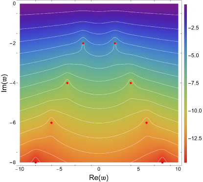
It is convenient and informative to present the pseudospectra as a contour plot in which the contour lines correspond to different values of . In the case of a normal operator these contour lines are concentric circles around the eigenvalues. In particular for sufficiently small the radius of the circle is also given by . This situation can be referred to as spectral stability. For non-normal operators however the contour lines are not necessarily circles. They can be much larger than circles of radius or even open lines in the complex plane. This indicates small perturbations can displace the eigenvalues of the operator by large amounts.
Let us have a look now to the pseudospectrum in our case. It is shown in figure 1. As one can see the contour lines are open. The colors indicate the values. Even tiny perturbations can completely destabilize the spectrum of quasinormal modes! It is important to note that this figure has been obtained with a discretization of the differential operator using pseudospectral methods at a grid size of points for . It turns out that the spectral instability gets stronger as the gridsize is increased. In fact one can argue that the resolvent does not converge to a finite value for (28). The reason is that the energy norm can not effectively exclude the modes which are outgoing from the horizon. These behave like near the horizon. The energy norm however only demands integrability on the horizon. In fact all functions which behave like the outgoing modes with have an integrable energy eq. 19. Therefore in the continuum limit all points with do belong to the spectrum of the operator acting on functions with finite energy (26).
4 Discussion
This result on the spectral instability of quasinormal modes is somewhat puzzling. After all we can construct the holographic Green’s function exactly and it does have a discrete set of poles in the complex plane. In contrast the spectrum of is continuous if it acts on functions with finite energy norm.
We note that, as we have emphasized, the definition of the holographic Green’s function implicitly relies on analytic continuation across the horizon. This analyticity requirement is much stronger than the requirement of existence of the energy norm. A way to circumvent this has been suggested in (26) and consists in replacing the energy norm by a Sobolev norm. In physicists terms this corresponds to higher order derivative terms in the norm. Higher derivative terms up to amount to lowering the limit for integrability to . In order to recover the exact spectrum one would of course have to take a limit with infinitely many derivatives. From the physics point of view the significance of such higher derivative terms is not clear.
Another line of thought could be that one considers the underlying theory (being it a scalar field, a Maxwell field or the metric itself) as an effective field theory valid down to a finite cutoff length scale . Then we would necessarily have some huge but finite value for determined e.g. by the criterion that the minimal distance between points of the discretization is larger than . Alternatively, one could also impose the boundary conditions not directly at the horizon but slightly outside at a sort of “stretched” horizon (29).
Finally let us close this overview by pointing to additional results on quasinormal modes in Anti-de Sitter space. The pseudospectrum in infalling Eddingtion-Finkelstein coordinates has been investigated in (30). One of the main findings was that in certain cases the pseudospectrum can significantly reach up into the upper halfplane giving rise to possible transient behaviour. Structural aspects of the pseudospectrum of quasinormal modes for AdS black holes have been pointed out and further investigated in (28). In particular the results in infalling Eddington-Finkelstein and regular coordinates have been contrasted. The properties of the pseudospectrum of black hole metrics have also been shown to give rise to transient behaviour for which a sum of quasinormal modes can be long lived of order in (31).
Funding
This work is supported through the grants CEX2020-001007-S and PID2021-123017NB-100, PID2021-127726NB-I00 funded by MCIN/AEI/10.13039/501100011033 and by ERDF “A way of making Europe”. The work of D.G.F. is supported by FPI grant PRE2022-101810.
Acknowledgments
We thank V. Boyanov and especially J. Jaramillo for numerous insightful discussions on the properties of quasinormal modes and their pseudospectra.
Conflict of Interest Statement
The authors declare that the research was conducted in the absence of any commercial or financial relationships that could be construed as a potential conflict of interest.
Author Contributions
All authors contributed equally.
References
- Maldacena (1998) Maldacena JM. The Large N limit of superconformal field theories and supergravity. Adv. Theor. Math. Phys. 2 (1998) 231–252. 10.4310/ATMP.1998.v2.n2.a1.
- Aharony et al. (2000) Aharony O, Gubser SS, Maldacena JM, Ooguri H, Oz Y. Large N field theories, string theory and gravity. Phys. Rept. 323 (2000) 183–386. 10.1016/S0370-1573(99)00083-6.
- Zaanen et al. (2015) Zaanen J, Sun YW, Liu Y, Schalm K. Holographic Duality in Condensed Matter Physics (Cambridge Univ. Press) (2015). 10.1017/CBO9781139942492.
- Ammon and Erdmenger (2015) Ammon M, Erdmenger J. Gauge/gravity duality: Foundations and applications (Cambridge: Cambridge University Press) (2015). 10.1017/CBO9780511846373.
- Breitenlohner and Freedman (1982) Breitenlohner P, Freedman DZ. Stability in Gauged Extended Supergravity. Annals Phys. 144 (1982) 249. 10.1016/0003-4916(82)90116-6.
- Son and Starinets (2002) Son DT, Starinets AO. Minkowski space correlators in AdS / CFT correspondence: Recipe and applications. JHEP 09 (2002) 042. 10.1088/1126-6708/2002/09/042.
- Gubser et al. (1996) Gubser SS, Klebanov IR, Peet AW. Entropy and temperature of black 3-branes. Phys. Rev. D 54 (1996) 3915–3919. 10.1103/PhysRevD.54.3915.
- Witten (1998) Witten E. Anti-de Sitter space, thermal phase transition, and confinement in gauge theories. Adv. Theor. Math. Phys. 2 (1998) 505–532. 10.4310/ATMP.1998.v2.n3.a3.
- Bellac (2011) Bellac ML. Thermal Field Theory. Cambridge Monographs on Mathematical Physics (Cambridge University Press) (2011). 10.1017/CBO9780511721700.
- Herzog and Son (2003) Herzog CP, Son DT. Schwinger-Keldysh propagators from AdS/CFT correspondence. JHEP 03 (2003) 046. 10.1088/1126-6708/2003/03/046.
- Horowitz and Hubeny (2000) Horowitz GT, Hubeny VE. Quasinormal modes of AdS black holes and the approach to thermal equilibrium. Phys. Rev. D 62 (2000) 024027. 10.1103/PhysRevD.62.024027.
- Birmingham et al. (2002) Birmingham D, Sachs I, Solodukhin SN. Conformal field theory interpretation of black hole quasinormal modes. Phys. Rev. Lett. 88 (2002) 151301. 10.1103/PhysRevLett.88.151301.
- Kovtun and Starinets (2005) Kovtun PK, Starinets AO. Quasinormal modes and holography. Phys. Rev. D 72 (2005) 086009. 10.1103/PhysRevD.72.086009.
- Policastro et al. (2002) Policastro G, Son DT, Starinets AO. From AdS / CFT correspondence to hydrodynamics. JHEP 09 (2002) 043. 10.1088/1126-6708/2002/09/043.
- Kovtun et al. (2005) Kovtun P, Son DT, Starinets AO. Viscosity in strongly interacting quantum field theories from black hole physics. Phys. Rev. Lett. 94 (2005) 111601. 10.1103/PhysRevLett.94.111601.
- Myers et al. (2007) Myers RC, Starinets AO, Thomson RM. Holographic spectral functions and diffusion constants for fundamental matter. JHEP 11 (2007) 091. 10.1088/1126-6708/2007/11/091.
- Trefethen (2000) Trefethen LN. Spectral methods in MATLAB (SIAM) (2000).
- Jaramillo et al. (2021) Jaramillo JL, Panosso Macedo R, Al Sheikh L. Pseudospectrum and Black Hole Quasinormal Mode Instability. Phys. Rev. X 11 (2021) 031003. 10.1103/PhysRevX.11.031003.
- Jaramillo et al. (2022) Jaramillo JL, Panosso Macedo R, Sheikh LA. Gravitational Wave Signatures of Black Hole Quasinormal Mode Instability. Phys. Rev. Lett. 128 (2022) 211102. 10.1103/PhysRevLett.128.211102.
- Destounis et al. (2021) Destounis K, Macedo RP, Berti E, Cardoso V, Jaramillo JL. Pseudospectrum of Reissner-Nordström black holes: Quasinormal mode instability and universality. Phys. Rev. D 104 (2021) 084091. 10.1103/PhysRevD.104.084091.
- Jaramillo (2022) Jaramillo JL. Pseudospectrum and binary black hole merger transients. Class. Quant. Grav. 39 (2022) 217002. 10.1088/1361-6382/ac8ddc.
- Gasperin and Jaramillo (2022) Gasperin E, Jaramillo JL. Energy scales and black hole pseudospectra: the structural role of the scalar product. Class. Quant. Grav. 39 (2022) 115010. 10.1088/1361-6382/ac5054.
- Boyanov et al. (2023) Boyanov V, Destounis K, Panosso Macedo R, Cardoso V, Jaramillo JL. Pseudospectrum of horizonless compact objects: A bootstrap instability mechanism. Phys. Rev. D 107 (2023) 064012. 10.1103/PhysRevD.107.064012.
- Courty et al. (2023) Courty A, Destounis K, Pani P. Spectral instability of quasinormal modes and strong cosmic censorship. Phys. Rev. D 108 (2023) 104027. 10.1103/PhysRevD.108.104027.
- Areán et al. (2023) Areán D, Fariña DG, Landsteiner K. Pseudospectra of holographic quasinormal modes. JHEP 12 (2023) 187. 10.1007/JHEP12(2023)187.
- Warnick (2015) Warnick CM. On quasinormal modes of asymptotically anti-de Sitter black holes. Commun. Math. Phys. 333 (2015) 959–1035. 10.1007/s00220-014-2171-1.
- Trefethen and Embree (2005) Trefethen LN, Embree M. Spectra and Pseudospectra: The Behavior of Nonnormal Matrices and Operators (Princeton University Press) (2005).
- Boyanov et al. (2024) Boyanov V, Cardoso V, Destounis K, Jaramillo JL, Panosso Macedo R. Structural aspects of the anti–de Sitter black hole pseudospectrum. Phys. Rev. D 109 (2024) 064068. 10.1103/PhysRevD.109.064068.
- Price and Thorne (1986) Price RH, Thorne KS. Membrane Viewpoint on Black Holes: Properties and Evolution of the Stretched Horizon. Phys. Rev. D 33 (1986) 915–941. 10.1103/PhysRevD.33.915.
- Cownden et al. (2024) Cownden B, Pantelidou C, Zilhão M. The pseudospectra of black holes in AdS. JHEP 05 (2024) 202. 10.1007/JHEP05(2024)202.
- Carballo and Withers (2024) Carballo J, Withers B. Transient dynamics of quasinormal mode sums (2024).
Figure captions