Shape Prior Segmentation Guided by Harmonic Beltrami Signature
Abstract
This paper presents a novel shape prior segmentation method guided by the Harmonic Beltrami Signature (HBS). The HBS is a shape representation fully capturing 2D simply connected shapes, exhibiting resilience against perturbations and invariance to translation, rotation, and scaling. The proposed method integrates the HBS within a quasi-conformal topology preserving segmentation framework, leveraging shape prior knowledge to significantly enhance segmentation performance, especially for low-quality or occluded images. The key innovation lies in the bifurcation of the optimization process into two iterative stages: 1) The computation of a quasi-conformal deformation map, which transforms the unit disk into the targeted segmentation area, driven by image data and other regularization terms; 2) The subsequent refinement of this map is contingent upon minimizing the distance between its Beltrami coefficient and the reference HBS. This shape-constrained refinement ensures that the segmentation adheres to the reference shape(s) by exploiting the inherent invariance, robustness, and discerning shape discriminative capabilities afforded by the HBS. Extensive experiments on synthetic and real-world images validate the method’s ability to improve segmentation accuracy over baselines, eliminate preprocessing requirements, resist noise corruption, and flexibly acquire and apply shape priors. Overall, the HBS segmentation framework offers an efficient strategy to robustly incorporate the shape prior knowledge, thereby advancing critical low-level vision tasks.
Key words: segmentation, shape prior, low-quality image processing, quasi-conformal, Harmonic Beltrami Signature
1 Introduction
Image segmentation stands as a cornerstone within the realm of computer vision, holding a pivotal role across diverse fields. Its essence lies in the precise localization of target objects within an image. Nonetheless, challenges such as poor image quality, occluded objects, blurred boundaries, and other complexities often impede segmentation efforts. In many instances, supplementary information exists regarding the shape of the target object, extending beyond what is directly discernible in the given image, commonly referred to as shape prior information. Integrating such prior knowledge into baseline segmentation algorithms represents a promising avenue for enhancing segmentation performance.
Over the past few decades, a multitude of algorithms for the shape prior segmentation have emerged. These approaches can be roughly classified into three categories based on the type of shape priors employed:
The first class uses geometric properties to describe target objects, such as convexity [29, 47, 20], local convexity [41], star shape [45], compactness [14], geodesic star [22], hedgehog [24], etc. While these methods can improve the performance of baseline algorithms on specific types of shapes, they obviously utilize only a limited portion of the shape information and struggle to differentiate further images sharing similar features.
The second class adopts a more intuitive approach, where researchers directly employ the target object’s boundary [5, 32, 40, 9, 17] or intensity [19, 12] as the shape prior. When dealing with a large number of template images, statistical techniques like PCA have been applied to better summarize the characteristics from the training set [48, 17, 40]. These approaches benefit from the ease of collecting training data and the strong interpretability of resulting shape priors. However, these methods require additional data preprocessing during training and inference, such as alignment, registration, and intensity remapping. The design of preprocessing significantly influences the obtained shape prior and consequently affects the final segmentation results.
The third class utilizes innovative shape representations, calculated based on the given images and capturing their specific features. These shape representations serve as shape priors [49]. Undoubtedly, the performance of the segmentation algorithm is significantly influenced by the representation, and thus, selecting a powerful representation is paramount.
The HBS [28] utilized in this paper is an instance of such a potent representation for 2D simply connected shapes. The HBS is uniquely determined by the given shape, invariant under translation, rotation, and scaling, and robust under small perturbations of the shape. The distance between different HBS can be measured easily by the norm because of the concise and unified form, a complex function defined on the unit disk. Notably, the original shape can be faithfully reconstructed from its corresponding HBS, indicating the comprehensive encapsulation of shape information within the signature. With the above advantages, the HBS can be integrated into the quasi-conformal topology preserving segmentation model [8] as a shape prior to guide the segmentation process and gain better performance, which becomes our novel HBS segmentation model.
To delve deeper, the result of the quasi-conformal segmentation model is a Beltrami coefficient, whereas the HBS is just an exceptional Beltrami coefficient. Such an intrinsic connection between the two motivates us to impose specific constraints on the quasi-conformal segmentation model, aligning the resultant Beltrami coefficient with an HBS. Concurrently, the boundary of the target object is extracted from the reference image, and then the corresponding HBS is computed as the shape prior. The option to utilize their average HBS is considered in scenarios where multiple images are provided. Subsequently, a comparison between the output Beltrami coefficient and the shape prior HBS is conducted by the norm, with iterative minimization to reduce their disparity. The incorporation of the HBS into our proposed model endows it with the following benefits:
-
1.
Our model ensures a certain level of similarity between the segmentation result and the reference shapes, leading to improved segmentation performance even for low-quality images;
-
2.
The invariance of HBS under translation, rotation, and scaling obviates the need for image preprocessing in our proposed model;
-
3.
The robustness of HBS against minor shape perturbations enhances the stability and reduces the sensitivity to noise in our model;
-
4.
The property of HBS preserving all shape information provides our model with a strong capability to discern target objects.
The rest of the paper is organized as follows: section 2 shows some related topics about shape prior segmentation; section 3 introduces some theoretical background; section 4 explains our proposed HBS segmentation model in detail; section 5 gives the numerical implementation; section 6 reports our experimental results; the paper is concluded in section 7, and we point out several future directions.
2 Related works
2.1 Traditional segmentation
Active contour or deformable models provide a practical framework for object segmentation and have been widely used in image segmentation. Kass et al. [25] first introduced the active contour method, evolving a contour towards object boundaries by minimizing an energy function. Osher et al. [35] and Sethian et al. [1] developed the level set method, using level sets of a higher dimensional function to enable the implicit representation of curves. The level set method quickly attracted researchers’ attention, and many related works have emerged, such as edge-based models [6, 7, 50], region-based models [33, 10], and shape prior models [27, 39]. It is worth noting that Chan et al. [10] enhanced the original level set model into a piecewise constant version, resulting in the well-known CV model, the first model to successfully reduce the heavy dependency on edge information.
Except for the active contour method, several baseline algorithms have been proposed. Graph cuts [4, 2, 3] formulate image segmentation as a minimum cut or maximum flow problem on a graph, where pixels are mapped to graph nodes and edges are weighted based on pairwise pixel similarities. The watershed transformation [38, 37, 13] segments images by treating intensity as a topographical surface and flooding from regional minima markers. -means [15, 36] clustering groups pixels into a predefined number of clusters based on feature similarity to perform segmentation. Mean shift [11, 44] is a nonparametric technique that finds density distribution modes to cluster pixels into homogeneous regions without predefined . The random walker algorithm [21, 16] simulates random walks from manually labeled seed pixels to probabilistically label other pixels for interactive segmentation.
2.2 Shape prior segmentation
Utilizing shape priors to guide segmentation is a highly viable approach for enhancing the performance of baseline algorithms, especially in complex scenarios. According to how people use shape priors, these methods can be categorized into three main groups.
Geometric features have caught some researchers’ attention, with convexity being one of the most popular properties among this category of shape prior segmentation methods. Gorelick et al. [20] utilized 3-clique potentials to penalize 1-0-1 configurations on straight lines and employed an efficient iterative trust region approach for optimization. Luo et al. [29] proposed a model incorporating convex multi-object segmentation using the signed distance function corresponding to their union and a Gaussian mixture method. Beyond convexity, properties such as compactness [14], star shape [45], geodesic star [22], hedgehog [24], and elliptical shape [43], can also effectively improve the segmentation accuracy and precision.
Conversely, an image’s boundary or intensity information is a valuable form of prior knowledge. Segmentation models under the level set framework can combine the shape prior distance components into their energy functions. Chan et al. [9] defined the shape distance by the Heaviside function of shapes and then put it into his CV model. Vu et al. [46] adopted a similar approach but normalized shapes based on their 3rd-order moments to reduce differences caused by variations in position and angle. Cootes et al. [12] treated the histogram of pixel density distribution within the target region as texture information and landmarks of the target shape as boundary information to guide segmentation.
Given plenty of template images, a statistical shape model(SSM) can generate a feature space and search for feasible segmentation within it. Malcolm et al. [32] uses kernel PCA to learn a statistical model of relevant shapes. Nakagomi et al. [34] proposed fully automated segmentation using multiple shape priors, which were selected from eigenshapes generated through the uniform sampling of the first two eigenmodes of an SSM. Saito et al. [40] proposed an algorithm that allows the selection of an optimal shape among the eigenshape space generated from SSM by conducting a branch-and-bound search and then does not require the construction of a hierarchical clustering tree before graph-cut segmentation. Yeo et al. [49] incorporated statistical shape information into the Bayesian formulation of the segmentation model using nonparametric shape density distribution. Eltanboly et al. [17] built SSM by modelling the empirical PDF for the intensity level distribution with a linear combination of Gaussians(LCG) and modified an Expectation-Maximization(EM) algorithm to handle the LCGs.
2.3 Quasi-conformal segmentation
The quasi-conformal theory has been widely used in the field of computer vision in recent years [54, 31, 23, 30, 58, 51, 56, 57, 55], and many segmentation algorithms based on it have significantly developed. Compared with the other methods, quasi-conformal segmentation is closely related to the proposed model, sharing a similar lineage. Chan et al. [8] proposed a new approach using the Beltrami representation of a shape for topology-preserving image segmentation. The topology of the segmentation result can be guaranteed by the given simple template by imposing only one constraint on the Beltrami representation, which can be handled easily. Subsequently, Siu et al. [42] began to focus on partial convexity in images and incorporated a registration-based segmentation model with a specially designed convexity constraint. Zhang et al. [52, 53] further expanded the application domain to 3D images and proposed segmentation models with the hyperelastic regularization and convexity regularization. Zhang et al. [56] combined quasi-conformal segmentation with a deep learning framework, designed a Topology-Preserving Segmentation Network(TPSN) and applied it in the field of medical imaging, which produced reliable results even in challenging cases.
3 Theoretical basis
3.1 Quasi-conformal mapping and Beltrami equation
A complex function is said to be quasi-conformal associated to if is orientation-preserving and satisfies the following Beltrami equation:
| (1) |
where is a complex-valued Lebesgue measurable function satisfying . More specifically, this is called the Beltrami coefficient of
| (2) |
In terms of the metric tensor, consider the effect of the pullback under of the Euclidean metric . The resulting metric is given by:
| (3) |
which, relative to the background Euclidean metric and , has eigenvalue and .
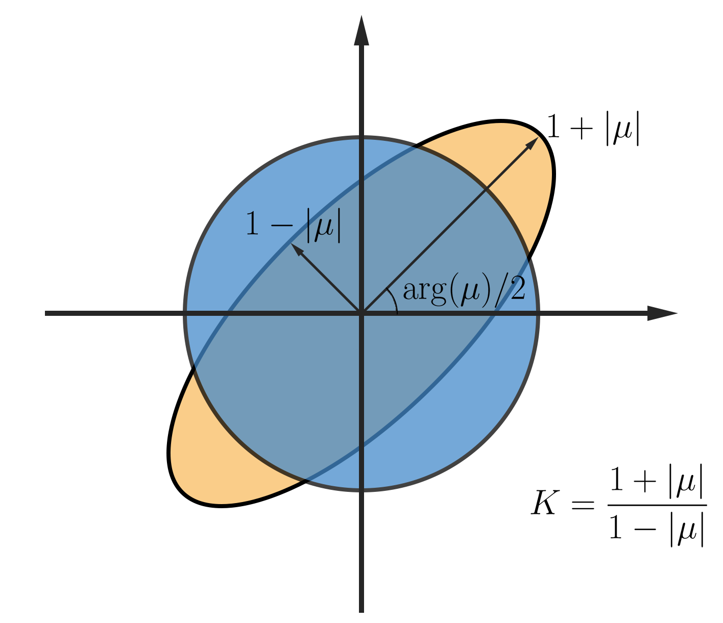
Therefore, inside the local parameter domain around some point , can be considered as a map composed of a translation to together with the multiplication of a stretch map and conformal function , which may be expressed as follows:
| (4) |
makes map a small circle to a small ellipse, and all the conformal distortion of is caused by . To form , we can determine the angles of the directions of maximal magnification and shrinkage and the amount of them as well. Specially, the angle of maximal magnification is with magnifying factor ; the angle of maximal shrinkage is the orthogonal angle with shrinkage factor . The distortion or dilation is given by:
| (5) |
Thus, the Beltrami coefficient gives us important information about the properties of the map (see fig. 1), and is a measure of non-conformality. In particular, the map is conformal around a small neighborhood of when and if everywhere on , us called conformal or holomorphic on .
Note that there is a one-to-one correspondence between the quasi-conformal mapping and its Beltrami coefficient . Given , there exists a Beltrami coefficient satisfying the Beltrami equation by equation eq. 2. Conversely, the following theorem states that given an admissible Beltrami coefficient , a quasi-conformal mapping always exists associated with this .
Theorem 1 (Measurable Riemannian Mapping Theorem)
Suppose is Lebesgue measurable satisfying ; then, there exists a quasi-conformal homeomorphism from onto itself, which is in the Sobolev space and satisfies the Beltrami equation in the distribution sense. The associated quasi-conformal homeomorphism is unique up to a Mobiüs transformation. Furthermore, by fixing , and , the is uniquely determined.
3.2 HBS
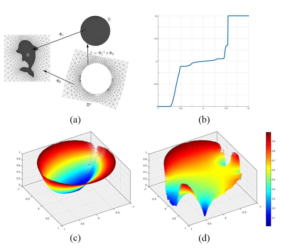
Suppose is a Jordan domain and a quasicircle. Let be the conformal welding of , where and are the conformal mappings. The harmonic extension of is achieved by the Poisson integral on the unit circle. Then the Beltrami coefficient of is called Generalized Harmonic Beltrami Signature (GHBS)
The process of obtaining GHBS is shown in fig. 2.
When the of GHBS satisfies , we call this GHBS fixed at infinity, and then the equivalence relation of GHBS can be defined as
Definition 1
Suppose two GHBS and are fixed at infinity, they are said to be equivalent if and , where and are respectively the harmonic extensions of a diffeomorphism and with is a Mobiüs transformation and is a rotation. In this case, we denote . Also, the equivalence class of is denoted by .
We consider the space of GHBS equivalence classes to study the quotient space of shapes , where , , iff and is composed of translation, rotation and scaling. The following theorem illustrates that GHBS is an effective representation.
Theorem 2
There is a one-to-one correspondence between and . In particular, given , its associated shape can be determined up to a translation, rotation, and scaling.
The Harmonic Beltrami Signature (HBS) is the unique representative of a GHBS equivalence class, which satisfies the following conditions:
| (6) | |||
| (7) | |||
| (8) |
Given shape , its HBS is uniquely determined and is invariant under rotation, translation, and scaling. The following theorem guarantees the geometric stability of HBS:
Theorem 3
Let , be two HBS and and be the normalized shapes associated to and respectively. If , then the Hausdorff distance between and satisfies
for some .
Besides, the effective reconstruction algorithm from an HBS to the original shape is also proposed and proved in [28]. This algorithm constructs a function such that and the Beltrami coefficient of is
4 Proposed segmentation model
This section describes our proposed shape prior segmentation model guided by HBS.
4.1 quasi-conformal topology preserving segmentation model
Recall the quasi-conformal topology preserving segmentation proposed by Chan [8], which is the fundamentation of our HBS segmentation model. Suppose are two regions, is an image, and is a binary template image. is called the topological template image defined as
| (9) |
where is the object region of . The key idea of this segmentation model is to find a quasi-conformal mapping which deforms the template to make it more similar to the given image , then the segmented target region is . Note that in most cases, we choose the rectangle domain .
This model can be formulated as the following energy functional:
| (10) |
where , is the Beltrami coefficient of , are weight parameters and is a generalized template image defined as
| (11) |
The first term of measures the difference between the deformed image and the template image . The second term limits the magnitude of since if and only if is quasi-conformal, which guarantees that is a diffeomorphism and that and are the same under topological sense. The last three terms are the regularization terms controlling the smoothness of . fig. 3 shows an example of the segmentation process and gives intuitive views of the variables of this model.
4.2 HBS as shape prior
The HBS is a signature of 2D simply connected shapes, and it represents the shape features by a complex function . More precisely, the HBS of given shape is the Beltrami coefficient of a HBS mapping , which is defined as
Definition 2
A quasi-conformal mapping is called HBS mapping if (1) its Beltrami coefficient is just the HBS of shape ; (2) where is conformal, is harmonic; (3) is conformal.
Indeed, the HBS provides a versatile and user-friendly shape representation. It eliminates the need for preprocessing tasks such as resizing and aligning, as well as the imposition of constraints on additional properties like convexity and curvature for input shapes.
The HBS is invariant under translation, rotation and scaling, which means it can be treated as a high-level shape prior with invariant geometric information. As is well-known, such transformations are widespread in image processing, and we have good reasons to believe that the HBS can effectively guide image segmentation.
In addition to those, HBS also possesses good stability. When two HBS are similar, their corresponding shapes only have minor differences, which is ensured by theorem 3. With this property, we can effortlessly extract common features as prior knowledge from the contours of many objects belonging to the same category by HBS. Here, we adopt the most straightforward method of computing the average HBS. Suppose we have shapes then their corresponding HBS can be computed as . We take the average HBS as the shape prior of this category. When only one shape exists, we employ its HBS directly.
4.3 HBS segmentation model
The primary objective of the segmentation model eq. 10 is to locate a suitable Beltrami coefficient , then the corresponding quasi-conformal function and the target region can be determined. While the HBS of the given shape is also a Beltrami coefficient of a HBS mapping such that . It is clear that the triplets of the HBS and of model eq. 10 exhibit incredibly high correlation. Inspired by their intrinsic connection, we integrate the HBS into the quasi-conformal topology preserving segmentation model as shape prior and propose a novel HBS segmentation model. Leveraging the excellent attributes of HBS, we can obtain an improved segmentation result that closely resembles the provided prior shape(s) even when dealing with low-quality images.
In order to better integrate them, we have also made the following modifications:
-
1.
Extend HBS: is defined on while is defined on . To solve the difference in the domain of definition, we require the image domain with as the center of and then extend to by , that is
(12) -
2.
Fix the template: The shape can be represented as in the HBS while the segmentation result is in model eq. 10. Therefore, we need to set the object region to be , and the template become
(13) -
3.
Add constraints: With the above modifications, , and are unified in form, which means they are both Beltrami coefficients of some quasi-conformal mappings on . A basic assumption in shape prior segmentation is that the ideal segmentation result should be similar to the prior shape . Moreover, theorem 3 provides a powerful tool to measure the distance between shapes by their HBS. However, this theorem is not suitable for , since only needs to be quasi-conformal in the original model eq. 10 instead of a HBS mapping. Unfortunately, the high complexity of the HBS algorithm makes it exceedingly difficult to entirely confine within the space formed by HBS mappings. Consequently, we have chosen to add a crucial constraint term into energy functional
(14) where imag(.) is the imaginary part of a complex number and is the Laplace operator. This term comes from the Fotiadis et al. [18] theorem:
Theorem 4
If the diffeomorphism satisfies the Beltrami equation
where , then can be equipped with a conformal metric such that is a harmonic map and the curvature of is given by
where is the conjugate harmonic function to .
Therefore, the HBS segmentation model is formulated as follows:
| (15) |
The first five terms directly come from model eq. 10 and play the same roles as before. The sixth term measures the similarity of the segmentation result and the given shape prior HBS. Furthermore, the last term with a big penalty parameter is a soft constraint that is almost an HBS mapping.
The term is crucial for proposed model eq. 15. For a given image , suppose that there is an ideal segmentation , whose HBS is , then we have
| (16) |
According to the basic assumption of shape prior segmentation, the given HBS is analogous to , which means is some small constant. Therefore, we can minimize the term to make segmentation result a good approximation of , which provides a simple yet effective method to utilize prior information for guiding the segmentation process.
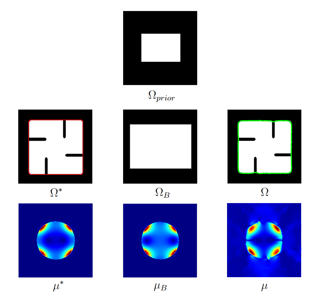
fig. 4 provides a visible example demonstrating how minimizing can induce a segmentation result similar to the unknown ideal segmentation . Several key points merit attention in this example:
-
1.
and represent the unknown ideal segmentation;
-
2.
is the shape obtained by translating, rotating and scaling to maximum the similarity to ;
-
3.
In practice, would never be computed but can be computed from ;
-
4.
Directly comparing with or even to achieve better results is not feasible since they visually differ from the ideal segmentation .
The following theorem guarantees the existence of the minimizer of model eq. 15 over .
Theorem 5
Proof: Following a similar argument in [26], we can show that is Cauchy complete and bounded, and hence compact. The four terms containing are obviously continuous over . Also, according to the Beltrami holomorphic flow and Bojarski theorem, the associated quasi-conformal map varies continuously (smoothly) under a continuous (smooth) variation of . Hence, the other terms are continuous over as well. Since is continuous on the compact set , has a minimizer in it.
Similar to that mentioned in [42], the smaller is, the more geometric distortion is allowed, and the deformed contour gets closer to the actual object boundary. However, small increases the difficulty of finding the minimizer, which is a trade-off between the accuracy and the efficiency. Meanwhile, the bigger is, the smoother the deformed contour is, but we get less accurate segmentation results. We can choose and according to the prior information of the given shape.
5 Numerical algorithm
In practice, a digital image consists of many pixels, which can be discrete using a triangular mesh , where is the set of vertices, is the edges between vertices, and is the set of triangle faces formed by edges. The deformation function is piecewise linear on each face and . The first derivative of is a piecewise constant, so the Beltrami coefficient is a constant on each face. Subsequently, is computed by averaging over the faces sharing the same vertex. A similar procedure is followed to compute . Although the input images are only defined on , we treat it as a continuous function through interpolation for the sake of convenience in the discussion. Hence, the deformed image can be achieved. As a result, the discrete HBS segmentation model is as follows:
| (17) |
However, this model implies a constraint , which presents a significant challenge during searching the minimizer. To address this, we disconnect the strong coupling between and and set another Beltrami coefficient without direct relation with as an alternative, which induces a weak HBS segmentation model:
| (18) |
Here we replace by in 2nd, 3th, 6th and 7th terms of model eq. 17 and add a new term to handle the difference between and , where is a big penalty parameter. If , will degenerate to .
This substitution allows us to split the original problem into two parts, and we call them subproblem
| (19) |
and subproblem
| (20) |
After such separation, these two subproblems have gained clearer and more practical meanings. The essence of the subproblem lies in determining the deformation mapping according to the pixel level difference and additional regularizations, then is achieved. Conversely, the target of the subproblem is to normalize the Beltrami coefficient obtained from the previous step under shape prior information for further segmentation. The soft constraint term bridges these two processes. Therefore, we can solve these two subproblems alternatively until they converge, which then gives the solution of the original optimization problem eq. 17.
More specifically, suppose and is obtained in -th iteration, then and can be computed by
| (21) |
| (22) |
The total algorithm is summarized in algorithm 2.
5.1 Solving subproblem
The target of subproblem is to find an optimal , but there are two additional input variables and in . Compared to solving for multiple variables simultaneously, it is simpler and more common to determine and in advance. Given , then is fixed and we can compute the minimizers explicitly by
| (23) |
where means the number of vertices inside the set. Except in necessary cases, we will omit all occurrences of and in the following discussion.
Even theorem 5 ensure the existence of minimizer, excessively large deformations can still burden the algorithm, lead to fluctuating segmentation results, and take long computation time. In -th iteration, instead of directly calculating , we attempt to compute a smaller deformation based on the previous segmentation result
| (24) |
where . Since is quasi-conformal then bijective, exists, we have
| (25) |
where is the deformed template image by and is the temporary segmentation result of after iterations. The approximate equality is due to the acceptable interpolation error, which decreases as the image resolution increases. Furthermore, this term can be expanded by a first-order Taylor series
| (26) |
where , is the discrete gradient of and is an operator for two complex number such that .
Since , the same interpolation approximation method in eq. 25 can be also applied to the other two regular terms of in eq. 19. Finally, subproblem can be rewritten in form about :
| (27) |
This is a quadratic optimization problem and can be solved according to Euler-Lagrange equation
| (28) |
subject to on . We mark the solution of eq. 28 in -th iteration as and the deform function is
| (29) |
Then the Beltrami coefficient can be computed by
| (30) |
To avoid some numerical errors, we designate if for some .
Besides, we also need for all to guarantee the deform function is quasi-conformal, so an additional truncation is applied to :
| (31) |
where is a small positive number. So far, we have addressed the subproblem and obtained the desired .
5.2 Solving subproblem
As mentioned before, subproblem eq. 20 essentially involves refining the solution obtained from the previous step. For any complex function and , we consider
| (32) |
Let , then is the argument of and . Let and , we have
| (33) |
According to the Green’s first identity, we have
where is the normal vector of . Since always holds on , we have and on . Therefore, the last two terms can be moved, and we get
| (34) |
Put it back to eq. 32, and we get gradient of with respect to as
| (35) |
After achieved, gradient desent method is applied to compute in -iteration of solving subproblem eq. 20, which is summarized in algorithm 1.
By the LBS method, we reconstruct the corresponding refined deform function from . That is, solve the following PDE:
| (36) |
The solution induces the temporary segmentation result and then is used in next iteration. Finally, we get the desired segmentation result when algorithm converges.
6 Experimental result
In this section, we demonstrate the effectiveness of the proposed HBS segmentation model through different experimental results. Our experiments are implemented using MATLAB R2014a running on 4-way Intel(R) Xeon(R) Gold 6230 processors with 80 cores at 2.10GHz base frequency and 1024 GB RAM under Ubuntu 18.04LTS 64-bit operating system.
6.1 Synthetic images
Deformation of the target object due to various reasons, such as image corruption, object occlusion, etc., is pervasive. In such cases, prior information can greatly assist us in making accurate segmentations. By utilizing HBS as the shape prior, the proposed segmentation model is aware of the approximate shape of the target object beforehand, leading to improved performance.
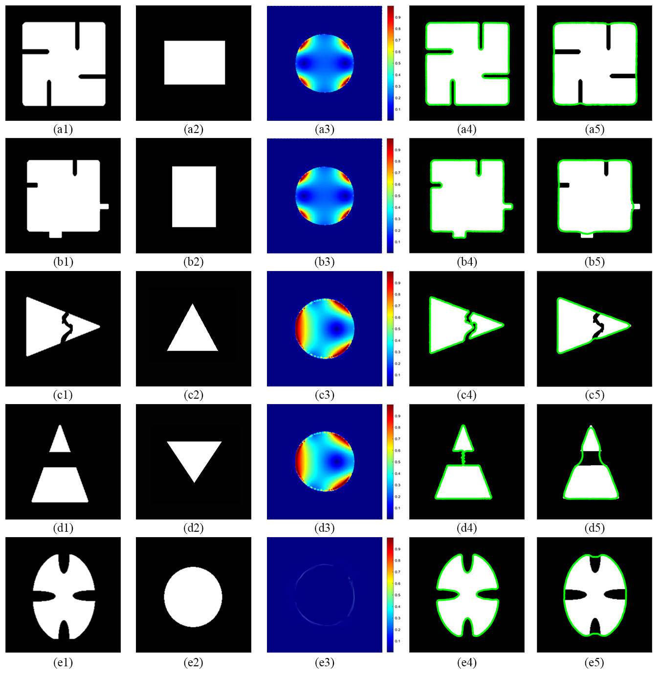
To illustrate this more intuitively, we have constructed a series of simple synthetic images to validate our model and display the results in fig. 5. For each row, the 1st column is the original shape, the 2nd column is the template shape, the 3rd column is the HBS corresponding to the template shape, the 4th column is the segmentation result without HBS, and the 5th column is the segmentation result of our proposed model. Before analyzing the results, it is essential to clarify some points, and we will use them in the following experiments unless otherwise specified.
-
1.
The template provided in the 2nd column is not in our model eq. 15, since has been fixed as the unit disk. Here, the template shape will not be fed into our model and is solely used to compute HBS in the 3rd column. We show them here to help our humans visually understand prior information.
-
2.
It is the magnitude of shown in the 3rd column to represent HBS.
-
3.
The green line in the 4th and 5th columns is the segmentation boundary.
- 4.
Let us look back on fig. 5, from which we can preliminarily obtain the following information:
-
1.
The HBS played a significant role in the low-quality image segmentation. We made some modifications to basic geometric shapes, resulting in them lacking certain parts, like subfigures (a1), (c1), (d1), and (e1), or having additional parts, like the bottom side and right side of subfigure (b1). We use such modifications as damage and occlusion to represent image degradation. Under the guidance of HBS, our model essentially disregarded the impact of these variations and provided satisfactory segmentation, which almost matched the given template. Meanwhile, the segmentation result without HBS is much more faithful to the actual shape boundaries.
-
2.
The proposed model can segment both the simply connected and multiply connected images and yield simply connected results. Although the HBS is the signature of simply-connected shapes, our model works well on multi-connected images in (c1) and (d1).
-
3.
The proposed model does not impose any requirements on the position, size, or orientation of the target object in the image. The HBS is invariant under translation, rotation, and scaling, and our model inherits this feature. With the same HBS, (a1) and (b1) are rectangles of different sizes, and our model can correctly segment them. Similarly, (c1) and (d1) are triangles in different orientations.
-
4.
The proposed model tolerates reasonable discrepancies between the prior information and the actual image. In experiment (e), the segmentation result is acceptable when the template is a circle, and the image is close to an ellipse.
-
5.
The proposed model effectively utilizes the prior information provided by the given template rather than simply extracting some basic geometric properties. In experiment (b), our model handles convex and concave parts at the same time.
-
6.
The final segmentation results can not strictly align with the provided templates but are inevitably influenced by the actual shape of the target region. For example, as shown in experiment (b), the rectangle in (b1) has notches at the top and left while protruding at the bottom and right. Therefore, the green curve representing the segmented boundary in (b5) is inward or outward at corresponding positions. Such situations are also noticeable in all other experiments.
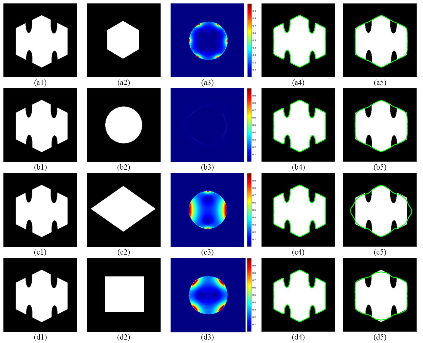
We will further observe the impact of different templates on the segmentation results from fig. 6. The meaning of each column is the same with fig. 5. The original image is similar to a hexagon, and we used hexagon (a2), round (b2), diamond (c2), and square (d2) as templates to segment it, with the results shown in (a5), (b5), (c5) and (d5) respectively. We can find that all segmentation results preserve some shape characteristics of their corresponding templates, but their performances differ significantly. The (a5) is the best, and (b5) is still acceptable, but (c5) and (d5) are far from accurate. That indicates our proposed method is highly sensitive to the given template. A precise template provides a perfect segmentation result, while an unsuitable template leads to a terrible one. On the other hand, it also implies that our model has a certain level of ability to understand prior information.
6.2 Natural images
The experimental results on synthetic images demonstrate that our model can effectively utilize prior information to segment partially damaged target objects. However, we are far from satisfied with this and have extended the model’s application to real-world images.
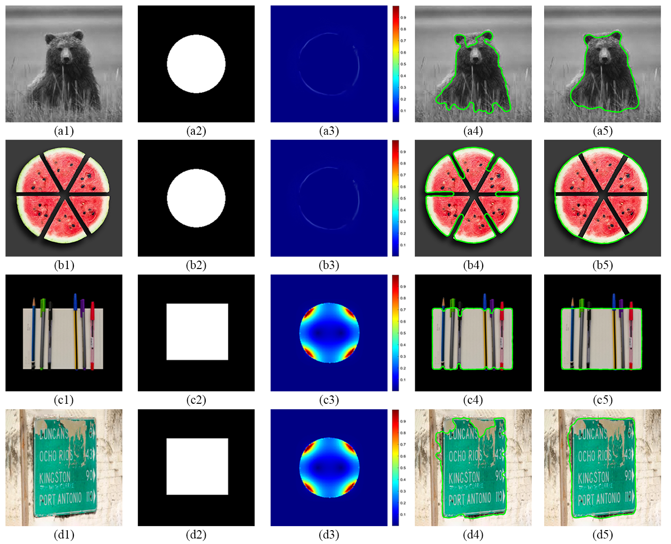
fig. 7 presents some results on natural images. As before, the original image, template, HBS, segmentation without HBS, and segmentation with HBS are sequentially displayed in columns 1 to 5 of each row.
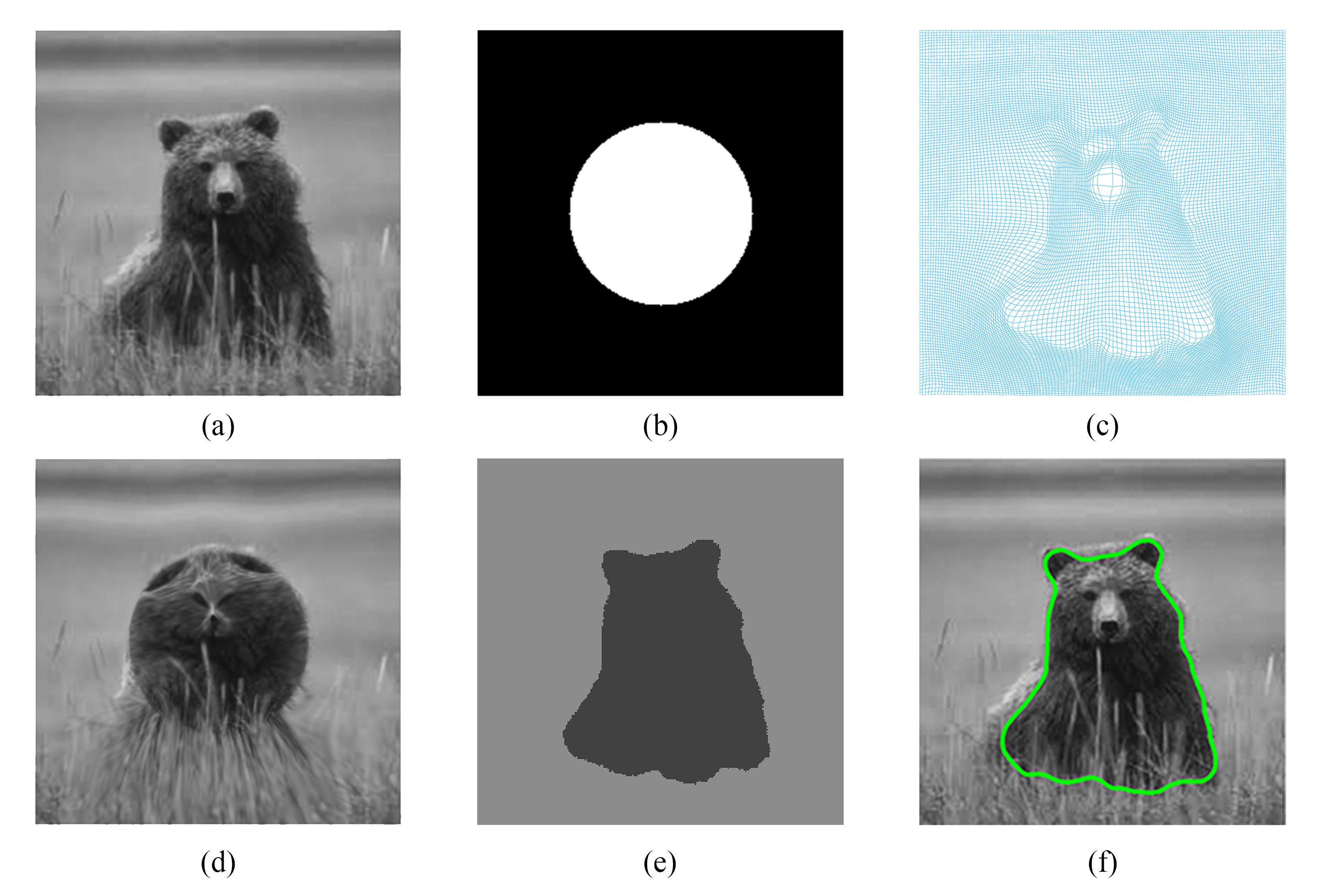
The first row (a1) is a grayscale image with a bear in grass. Without HBS, the model only relies on the intensity of grayscale values to determine the shape boundaries (a4), which results in the top boundary being limited to the brighter forehead and the bottom boundary appearing jagged due to the grass. When HBS is specified, even if the circle is not a suitable template, it helps our proposed HBS segmentation model generate a much smoother and more complete result (a5). The other three images are color images, which must be compressed RGB to grayscale value before applying our model. The result (b5) demonstrates that no matter how many pieces the target object is separated into, our model can segment it as a simply connected entity, just like it does on synthetic images. The experiment (c) represents a similar but more practical scenario, occlusion, and our model successfully and accurately identifies the white paper behind pens in (c5). In (d5), our model also locates the signboard partially covered under the dust.
6.3 Segmentation process
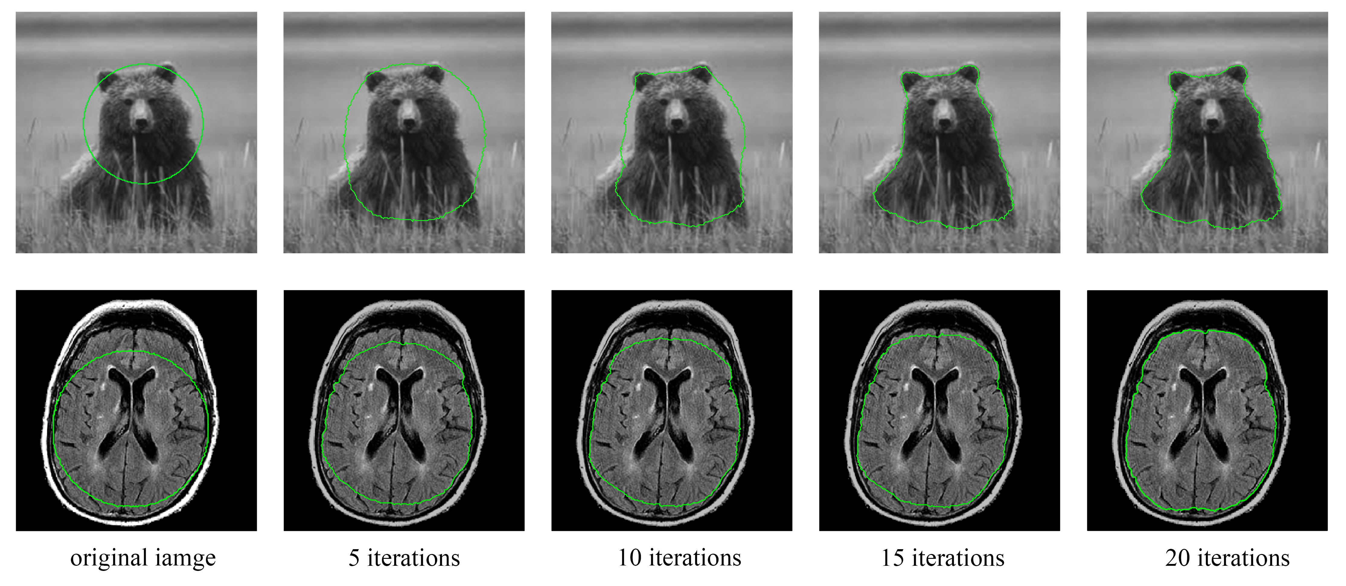
The proposed method utilizes an iterative process to progressively deform an initial circular segmentation template into the final segmentation result, as described in section 5.1. This iterative deformation procedure was experimentally investigated, with results demonstrated in fig. 8. The segmentation progression on images of a bear and a brain is shown in the first and second rows, respectively. The initial circular template position is depicted in green in the first column. The intermediate temporary segmentation results after 5, 10, 15, and 20 iterations are displayed in green in the subsequent columns.
This experiment clearly exhibits the smooth deformation of the segmentation results across iterations, supporting the stability of the proposed iterative algorithm. Additionally, the convergence rate of the algorithm depends on several factors, including image complexity, resolution, HBS selection, step size, initial template position, and so on. For instance, the bear segmentation nears convergence after 15 iterations, while the brain segmentation still demonstrates significant differences between the 15th and 20th iterations. The algorithm typically converges within approximately 20 iterations under a suitable parameter setting, yielding satisfactory segmentation outcomes. In summary, this analysis of the iterative deformation process provides insights into the stability and convergence properties of the proposed HBS segmentation approach.
6.4 Impact of initial position
Our model is a region-based segmentation method developed from the CV model. Thus, it shares common characteristics with algorithms of this category: it is sensitive to the initial position. In our model, the initial shape is fixed as a circle, and we need to set the center and radius to determine the initial position before the algorithm iteration begins.
We conducted a detailed investigation into the impact of the initial position on the segmentation results, as illustrated in fig. 9. The image used for segmentation contains three circles, with the large white circle in the lower-left corner partially overlapping the smaller gray circle. In contrast, the third circle is far away in the upper-right corner. We try 11 different typical initial positions and obtain the corresponding results.
As shown in (a), (b), and (c), when the initial circle is entirely within the target shape, we can achieve highly accurate segmentation results even in cases with overlapping regions. Meanwhile, (e), (f), and (g) indicate that when the initial circle contains the whole of the target region, the proposed model also generated reliable segmentation but may be affected by nearby objects. The inference of adjacent objects can be clearly observed in the comparison between (a2) and (e2), (b2) and (f2). In (i) and (j), we display the stable results under offsets of the initial circle. At the same time, we focus on the overlapping region in (k), whose segmented region (k2) does not grow continuously to fully encompass both circles, as is common in other algorithms. Instead, it is constrained by HBS and stops iterating, resulting in an outcome that does not conform to any edge. The segmented region of (d2) undergoes significant deformation and encompasses all three circles. However, the boundaries within the black background area still roughly resemble a circular shape, where such constraints of HBS are also evident. Finally, no meaningful segmentation is obtained if the initial position is set in an empty area as (h).
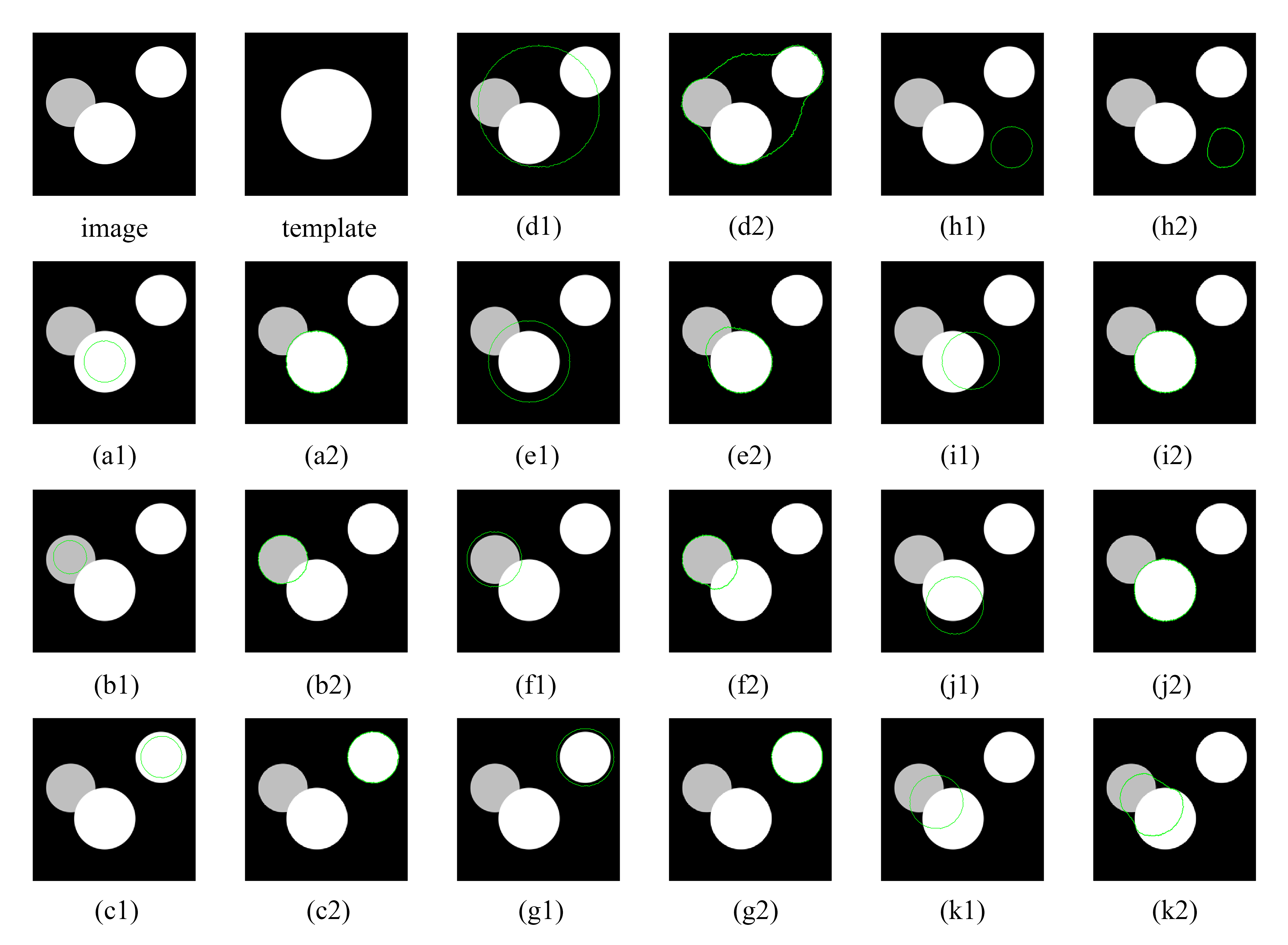
In summary, the above experiments show that the proposed model can accurately locate the target regions based on the initial position. Additionally, we do not require precise initial position settings since the model is relatively insensitive and can accommodate reasonable offset and scaling of the initial circle. However, an inappropriate starting may yield an unexpected outcome. As mentioned earlier in section 6.1, the segmentation results can be influenced by adjacent objects, so avoiding other objects can help improve the segmentation performance.
6.5 Segmentation on noised images
Image degradation is ubiquitous in real-world computer vision applications, but segmentation of such low-quality images remains challenging. When algorithms falter in the presence of noise, their applicability diminishes substantially. Thus, advancing robust segmentation for corrupted images is essential. Shape priors could play a crucial role in this context by furnishing informative constraints during the processing pipeline.
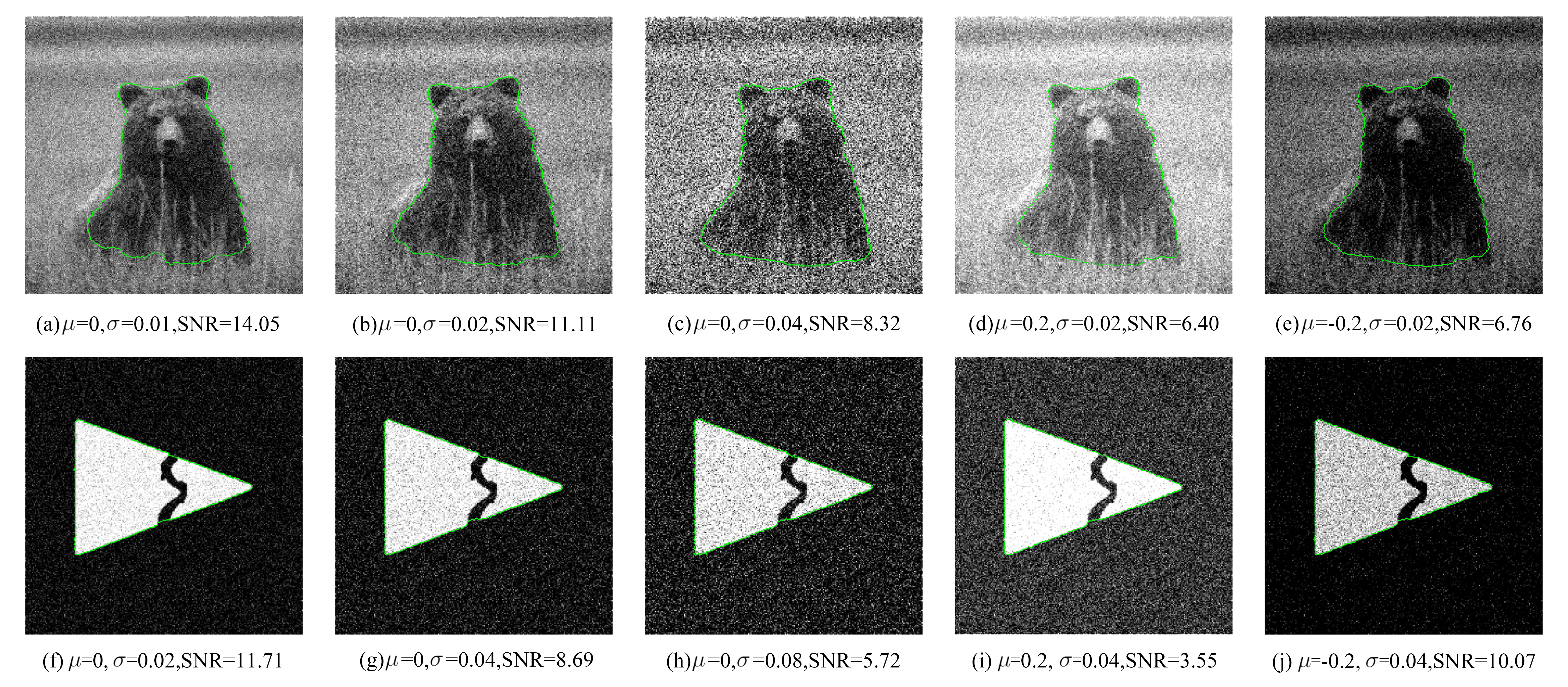
The following experiment demonstrates that our HBS segmentation allows for accurate analysis even when images are severely degraded by noise. In fig. 10, we add Gaussian noise with mean and variance to natural and synthetic images to simulate image degradation. The parameters of Gaussian noise and Signal to Noise Ratio(SNR) are marked under each subfigure. For the bear in 1st row, the clear original image and its segmentation result are displayed in fig. 7 (a1) and (a5). For the split triangle in the 2nd row, the clear original image and segmentation result are (c1) and (c5) of fig. 5.
It is evident that as the intensity of noise increases, the segmentation task becomes progressively more challenging, inevitably resulting in less smooth boundaries. However, leveraging HBS enables us to achieve relatively stable segmentation results. This effect is conspicuous in (a2) and (a3), where noticeable jagged edges emerge on both sides of the bear’s head.
Furthermore, the tolerance of our proposed algorithm to noise fluctuates depending on the complexity of the image. For the split triangle, the segmentation performance remains good when in (h). However, the algorithm can not handle effectively for bear.
6.6 Enhancing object segmentation in multiple components scenes
In reality, objects often have complex shapes with multiple components. For example, a house may feature a pentagonal outline, a triangular roof, rectangular doors, and circular windows. Accurately identifying and isolating the desired region amidst these intricate boundaries is challenging. The HBS effectively captures shape features and demonstrates strong object recognition capabilities, making it suitable for classification tasks. Therefore, using HBS to provide additional shape prior information offers a promising approach for segmenting specific areas in images with diverse components.
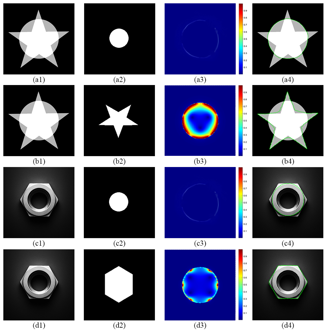
fig. 11 is an attempt under situations described above and provides two sets of examples. The first set is tested on a synthetic image comprising a highly overlapping semi-transparent circle and pentagram. In this case, we aim to locate the circle and the pentagram, as shown in rows (a) and (b). The second set is tested on a hexagonal nut with an annular protrusion, and we attempt to segment the inner protrusion contour and the overall outline of the nut, as displayed in rows (c) and (d). The results (a4) to (d4) in the last column effectively demonstrate our model’s ability, with the assistance of HBS, to accurately locate the target object in an image with multiple components according to the given requirements.
6.7 Shape prior of object(s) with complicated boundary
We have illustrated that shape prior can help segmentation, but obtaining shape prior remains a problem. In previous experiments, the templates fed into our model were always simple geometric shapes such as circles, triangles, etc. Although these simple shapes allow our model to achieve good results, they conceal the enormous potential of the HBS segmentation model.
While basic geometric shapes can be described using straightforward signatures like area, density, curvature, and circularity, their effectiveness diminishes as the complexity of the object increases. In such cases, traditional signatures struggle to capture the shape information fully, highlighting the capacity of the HBS to represent intricate shapes effectively. The HBS uses a simple and unified form to fully encode the characteristics of shapes, exhibiting a range of wonderful properties and enabling the reconstruction of the original shapes. Apart from extracting the shape boundaries, the HBS does not require any additional preprocessing to the image, which makes it extremely easy to find standard features from a large number of images of the same object class.
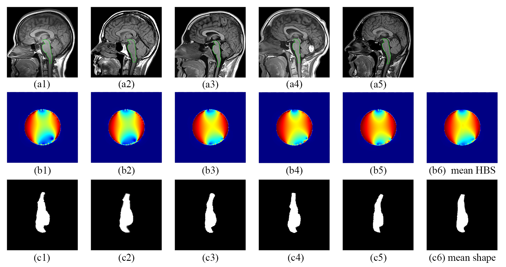
In the medical field, physiological structures often exhibit specific shapes. Still, these shapes are complex and have a certain degree of variability, making their features hard to describe mathematically with clarity. fig. 12 provides an example of computing shape prior of brains. (a1) to (a6) are the images of the brains with green lines as their boundary, (b1) to (b6) show their corresponding HBS, and (c1) to (c6) display the reconstructed brains from HBS. We can observe a small gap between the given brains in the 1st row and the reconstructed brains in the 3rd row, which is actually due to the resolution. However, it does not affect our segmentation since the reconstructed results are not used in our segmentation model at all. Besides, this gap will decrease when the resolution increases, as mentioned in [28].
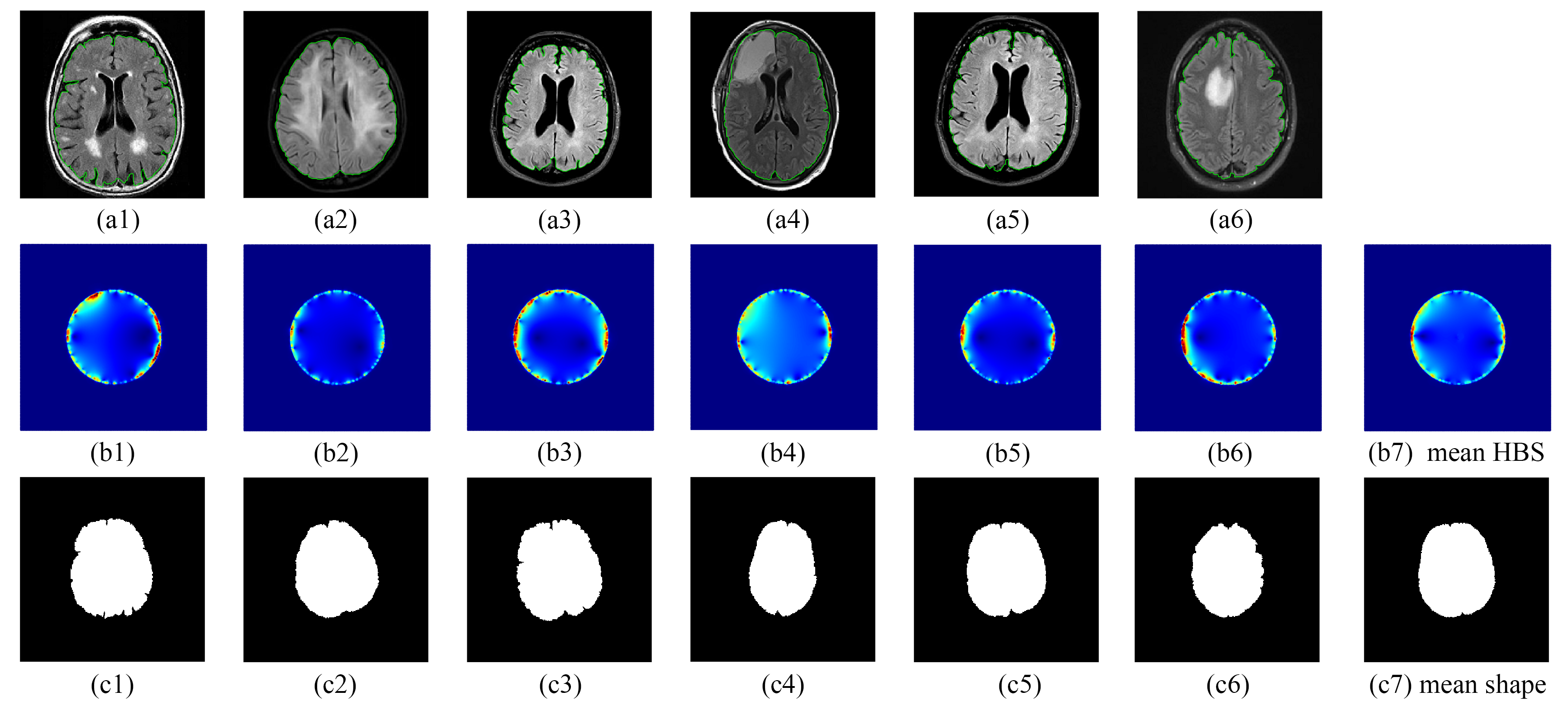
Then we directly calculate the algebraic mean of the HBS of the above six brains, called the mean HBS, and also reconstruct a brain from the mean HBS, called the mean shape, which are respectively shown in the (b7) and (c7). Even though the relationship between HBS and the shape is challenging to explain, we can still observe the following features from (b1) to (b6):
-
1.
The majority of HBS values are small since brains appear roughly like circles.
-
2.
The HBS has larger values on the left side and smaller values on the right side, indicating a slightly tapering shape resembling the human brain.
-
3.
The HBS exhibits scattered high values along its boundary, corresponding to the sulcus in the brain’s outline.
The mean HBS also preserves these features, but the high values on the boundary become much less and are mainly concentrated at the left and right ends. This is reflected in the mean shape (c7), which has a smoother outline with distinct inward curvatures at the division between the left and right halves of the brain. Because of that, we believe that the mean HBS serves as a good shape prior.
It is noteworthy that utilizing the mean HBS as shape prior is not trivial, despite the fact that the mean HBS (b7) is exactly the HBS of the mean shape (c7). Achieving the mean shape directly poses challenges due to significant differences among shapes, such as variations in size, position, and angle. For example, prior to calculating the mean shape, brains (a1) to (a6) differ and are required to be realigned, resized, and oriented accordingly under traditional methods. Besides, all of the above operations rely on specific feature points, whose rationality and universality are also crucial factors to consider. In contrast, the HBS can circumvent these geometric discrepancies and capture potential shape features effectively. In summary, the mean HBS provides a generic and convenient method to extract shape prior with a solid theoretical background.
6.8 Segmentation of complex image(s)
With the help of the mean HBS, we can now apply our proposed segmentation model to complex images with suitable shape prior. Firstly, We take some new brains and the mean HBS in the last experiment as an example. For each row in fig. 13, the 1st column is the given brain, the 2nd column is the segmentation result without HBS, the 3rd column is the segmentation result guided by the HBS of unit disk and the 4th column is the segmentation result guided by the mean HBS shown in (b7) of fig. 12.
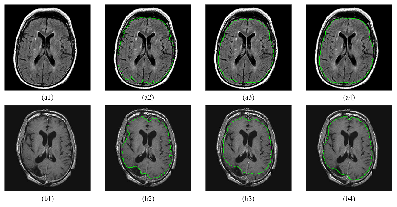
In fig. 13, the brain (a1) is quite similar to those used to compute mean HBS, (a1) to (a6) of fig. 12, leading that the result (a4) guided by mean HBS is almost perfect. The result (a3), guided by the HBS of the unit disk, loses some top and bottom regions, which makes it more circular. And the result (a2) without HBS has a very rough boundary. Due to some deep sulcus, it tends to discard regions with relatively discontinuous intensity, like the small part on the bottom of the brain. The brain (b1) in the second row has a pathological region in the left bottom corner that deviates from our summarized standard features. Therefore, the segmentation result (b4) with mean HBS provides a relatively smooth and continuous contour while attempting to make up the missing region. This is precisely the desired outcome: areas affected by lesions or atrophy are still considered part of the brain. However, the other two results, (b2) and (b3), are not satisfactory enough and exhibit similar shortages with their corresponding ones in row (a).
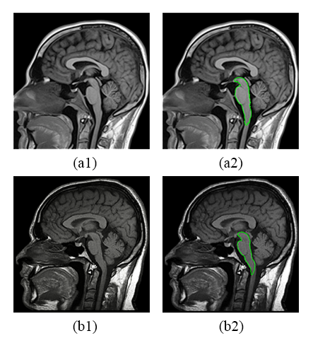
We also conducted similar experiments on the brainstem and achieved favorable results. fig. 14 displays the mean HBS (b6) extracted from (a1) to (a5), while fig. 15 illustrates the application of mean HBS for segmenting some new brainstem images (a1) and (b1).
7 Conclusion
This paper introduces a novel segmentation model leveraging HBS as shape prior. The key contributions and conclusions are summarized as follows:
-
1.
We integrated the HBS into the quasi-conformal segmentation framework as a shape prior term, where the HBS guides the segmentation towards shapes similar to the provided prior.
-
2.
The HBS prior eliminates requirements for alignment, resizing, and orientation of shapes, and our HBS segmentation model naturally inherits such properties.
-
3.
Experiments on synthetic and natural images exhibited substantial improvements over the baseline model without HBS, validating the benefits of HBS in dealing with image degradation, occlusion, low contrast, and high noise.
-
4.
Segmentation results demonstrated accurate object localization in multi-part images by selecting an appropriate HBS prior, showing strong shape-discerning capabilities.
-
5.
Using the mean HBS computed from many related shapes provides an effective technique for obtaining a suitable shape prior, which is very useful for segmenting complicated images.
In conclusion, the HBS prior segmentation model provides a novel, efficient, and flexible strategy to incorporate shape knowledge into segmentation algorithms. Substantial performance gains verify the advantages of the HBS representation. This paper illustrates the significant potential of HBS-guided techniques to advance a wide range of shape analysis tasks. Future work may explore HBS-based priors for 3D shapes and integrate the model into deep neural networks.
Acknowledgement
This work is supported by HKRGC GRF (Project ID: 14307622).
References
- [1] David Adalsteinsson and James A Sethian. A fast level set method for propagating interfaces. Journal of computational physics, 118(2):269–277, 1995.
- [2] Reinhard Beichel, Alexander Bornik, Christian Bauer, and Erich Sorantin. Liver segmentation in contrast enhanced ct data using graph cuts and interactive 3d segmentation refinement methods. Medical physics, 39(3):1361–1373, 2012.
- [3] Yuri Boykov and Gareth Funka-Lea. Graph cuts and efficient nd image segmentation. International journal of computer vision, 70(2):109–131, 2006.
- [4] Yuri Y Boykov and M-P Jolly. Interactive graph cuts for optimal boundary & region segmentation of objects in nd images. In Proceedings eighth IEEE international conference on computer vision. ICCV 2001, volume 1, pages 105–112. IEEE, 2001.
- [5] Xavier Bresson, Pierre Vandergheynst, and Jean-Philippe Thiran. A Variational Model for Object Segmentation Using Boundary Information and Shape Prior Driven by the Mumford-Shah Functional. International Journal of Computer Vision, 68(2):145–162, June 2006.
- [6] Vicent Caselles, Francine Catté, Tomeu Coll, and Françoise Dibos. A geometric model for active contours in image processing. Numerische mathematik, 66:1–31, 1993.
- [7] Vicent Caselles, Ron Kimmel, and Guillermo Sapiro. Geodesic active contours. In Proceedings of IEEE international conference on computer vision, pages 694–699. IEEE, 1995.
- [8] Hei-Long Chan, Shi Yan, Lok-Ming Lui, and Xue-Cheng Tai. Topology-Preserving Image Segmentation by Beltrami Representation of Shapes. Journal of Mathematical Imaging and Vision, 60(3):401–421, March 2018.
- [9] T. Chan and W. Zhu. Level Set Based Shape Prior Segmentation. In 2005 IEEE Computer Society Conference on Computer Vision and Pattern Recognition (CVPR’05), volume 2, pages 1164–1170, San Diego, CA, USA, 2005. IEEE.
- [10] Tony F Chan and Luminita A Vese. Active contours without edges. IEEE Transactions on image processing, 10(2):266–277, 2001.
- [11] Dorin Comaniciu and Peter Meer. Mean shift analysis and applications. In Proceedings of the seventh IEEE international conference on computer vision, volume 2, pages 1197–1203. IEEE, 1999.
- [12] Tim F. Cootes and Christopher J. Taylor. Statistical models of appearance for medical image analysis and computer vision. In Milan Sonka and Kenneth M. Hanson, editors, Medical Imaging 2001, pages 236–248, San Diego, CA, July 2001.
- [13] Jean Cousty, Gilles Bertrand, Laurent Najman, and Michel Couprie. Watershed cuts: Minimum spanning forests and the drop of water principle. IEEE transactions on pattern analysis and machine intelligence, 31(8):1362–1374, 2008.
- [14] Piali Das, Olga Veksler, Vyacheslav Zavadsky, and Yuri Boykov. Semiautomatic segmentation with compact shape prior. Image and Vision Computing, 27(1-2):206–219, 2009.
- [15] Nameirakpam Dhanachandra, Khumanthem Manglem, and Yambem Jina Chanu. Image segmentation using k-means clustering algorithm and subtractive clustering algorithm. Procedia Computer Science, 54:764–771, 2015.
- [16] Xingping Dong, Jianbing Shen, Ling Shao, and Luc Van Gool. Sub-markov random walk for image segmentation. IEEE Transactions on Image Processing, 25(2):516–527, 2015.
- [17] Ahmed Eltanboly, Mohammed Ghazal, Hassan Hajjdiab, Ahmed Shalaby, Andy Switala, Ali Mahmoud, Prasanna Sahoo, Magdi El-Azab, and Ayman El-Baz. Level sets-based image segmentation approach using statistical shape priors. Applied Mathematics and Computation, 340:164–179, January 2019.
- [18] Anestis Fotiadis and Costas Daskaloyannis. Beltrami equation for the harmonic diffeomorphisms between surfaces. Nonlinear Analysis, 214:112546, 2022.
- [19] D. Freedman and Tao Zhang. Interactive Graph Cut Based Segmentation with Shape Priors. In 2005 IEEE Computer Society Conference on Computer Vision and Pattern Recognition (CVPR’05), volume 1, pages 755–762, San Diego, CA, USA, 2005. IEEE.
- [20] Lena Gorelick, Olga Veksler, Yuri Boykov, and Claudia Nieuwenhuis. Convexity Shape Prior for Binary Segmentation. IEEE Transactions on Pattern Analysis and Machine Intelligence, 39(2):258–271, February 2017.
- [21] Leo Grady. Random walks for image segmentation. IEEE transactions on pattern analysis and machine intelligence, 28(11):1768–1783, 2006.
- [22] Varun Gulshan, Carsten Rother, Antonio Criminisi, Andrew Blake, and Andrew Zisserman. Geodesic star convexity for interactive image segmentation. In 2010 IEEE Computer Society Conference on Computer Vision and Pattern Recognition, pages 3129–3136. IEEE, 2010.
- [23] Yuchen Guo, Qiguang Chen, Gary PT Choi, and Lok Ming Lui. Automatic landmark detection and registration of brain cortical surfaces via quasi-conformal geometry and convolutional neural networks. Computers in Biology and Medicine, 163:107185, 2023.
- [24] Hossam Isack, Olga Veksler, Milan Sonka, and Yuri Boykov. Hedgehog shape priors for multi-object segmentation. In Proceedings of the IEEE Conference on Computer Vision and Pattern Recognition, pages 2434–2442, 2016.
- [25] Michael Kass, Andrew Witkin, and Demetri Terzopoulos. Snakes: Active contour models. International Journal of Computer Vision, 1(4):321–331, January 1988.
- [26] Ka Chun Lam and Lok Ming Lui. Landmark-and intensity-based registration with large deformations via quasi-conformal maps. SIAM Journal on Imaging Sciences, 7(4):2364–2392, 2014.
- [27] Michael E Leventon, W Eric L Grimson, and Olivier Faugeras. Statistical shape influence in geodesic active contours. In 5th IEEE EMBS International Summer School on Biomedical Imaging, 2002., pages 8–pp. IEEE, 2002.
- [28] Chenran Lin and Lok Ming Lui. Harmonic Beltrami Signature: A Novel 2D Shape Representation for Object Classification. SIAM Journal on Imaging Sciences, 15(4):1851–1893, December 2022.
- [29] Shousheng Luo, Xue-Cheng Tai, Limei Huo, Yang Wang, and Roland Glowinski. Convex Shape Prior for Multi-Object Segmentation Using a Single Level Set Function. In 2019 IEEE/CVF International Conference on Computer Vision (ICCV), pages 613–621, Seoul, Korea (South), October 2019. IEEE.
- [30] Zhiyuan Lyu, Qiguang Chen, and Lok Ming Lui. A two-stage algorithm for combined quasiconformal and optimal mass transportation spherical parameterization. Mathematics, Computation and Geometry of Data, 3(1):29–57, 2023.
- [31] Zhiyuan Lyu, Lok Ming Lui, and Gary P. T. Choi. Spherical density-equalizing map for genus-0 closed surfaces, 2024.
- [32] James Malcolm, Yogesh Rathi, and Allen Tannenbaum. Graph Cut Segmentation with Nonlinear Shape Priors. In 2007 IEEE International Conference on Image Processing, pages IV – 365–IV – 368, San Antonio, TX, USA, 2007. IEEE.
- [33] David Bryant Mumford and Jayant Shah. Optimal approximations by piecewise smooth functions and associated variational problems. Communications on pure and applied mathematics, 1989.
- [34] Keita Nakagomi, Akinobu Shimizu, Hidefumi Kobatake, Masahiro Yakami, Koji Fujimoto, and Kaori Togashi. Multi-shape graph cuts with neighbor prior constraints and its application to lung segmentation from a chest ct volume. Medical image analysis, 17(1):62–77, 2013.
- [35] Stanley Osher and James A Sethian. Fronts propagating with curvature-dependent speed: Algorithms based on hamilton-jacobi formulations. Journal of computational physics, 79(1):12–49, 1988.
- [36] Thrasyvoulos N Pappas and Nikil S Jayant. An adaptive clustering algorithm for image segmentation. In International Conference on Acoustics, Speech, and Signal Processing,, pages 1667–1670. IEEE, 1989.
- [37] K Parvati, Prakasa Rao, M Mariya Das, et al. Image segmentation using gray-scale morphology and marker-controlled watershed transformation. Discrete Dynamics in Nature and Society, 2008, 2008.
- [38] Jos BTM Roerdink and Arnold Meijster. The watershed transform: Definitions, algorithms and parallelization strategies. Fundamenta informaticae, 41(1-2):187–228, 2000.
- [39] Mikael Rousson and Nikos Paragios. Shape priors for level set representations. In Computer Vision—ECCV 2002: 7th European Conference on Computer Vision Copenhagen, Denmark, May 28–31, 2002 Proceedings, Part II 7, pages 78–92. Springer, 2002.
- [40] Atsushi Saito, Shigeru Nawano, and Akinobu Shimizu. Joint optimization of segmentation and shape prior from level-set-based statistical shape model, and its application to the automated segmentation of abdominal organs. Medical Image Analysis, 28:46–65, February 2016.
- [41] Chun Yin Siu, Hei Long Chan, and Ronald Lok Ming Lui. Image Segmentation with Partial Convexity Shape Prior Using Discrete Conformality Structures. SIAM Journal on Imaging Sciences, 13(4):2105–2139, January 2020.
- [42] Chun Yin Siu, Hei Long Chan, and Ronald Lok Ming Lui. Image segmentation with partial convexity shape prior using discrete conformality structures. SIAM Journal on Imaging Sciences, 13(4):2105–2139, 2020.
- [43] G. Slabaugh and G. Unal. Graph cuts segmentation using an elliptical shape prior. In IEEE International Conference on Image Processing 2005, pages II–1222, Genova, Italy, 2005. IEEE.
- [44] Wenbing Tao, Hai Jin, and Yimin Zhang. Color image segmentation based on mean shift and normalized cuts. IEEE Transactions on Systems, Man, and Cybernetics, Part B (Cybernetics), 37(5):1382–1389, 2007.
- [45] Olga Veksler. Star shape prior for graph-cut image segmentation. In Computer Vision–ECCV 2008: 10th European Conference on Computer Vision, Marseille, France, October 12-18, 2008, Proceedings, Part III 10, pages 454–467. Springer, 2008.
- [46] Nhat Vu and B.S. Manjunath. Shape prior segmentation of multiple objects with graph cuts. In 2008 IEEE Conference on Computer Vision and Pattern Recognition, pages 1–8, Anchorage, AK, USA, June 2008. IEEE.
- [47] Shi Yan, Xue-Cheng Tai, Jun Liu, and Hai-Yang Huang. Convexity Shape Prior for Level Set-Based Image Segmentation Method. IEEE Transactions on Image Processing, 29:7141–7152, 2020.
- [48] Yunyun Yang, Xiu Shu, Ruofan Wang, Chong Feng, and Wenjing Jia. Parallelizable and robust image segmentation model based on the shape prior information. Applied Mathematical Modelling, 83:357–370, July 2020.
- [49] Si Yong Yeo, Xianghua Xie, Igor Sazonov, and Perumal Nithiarasu. Segmentation of biomedical images using active contour model with robust image feature and shape prior. International Journal for Numerical Methods in Biomedical Engineering, 30(2):232–248, February 2014.
- [50] Anthony Yezzi, Satyanad Kichenassamy, Arun Kumar, Peter Olver, and Allen Tannenbaum. A geometric snake model for segmentation of medical imagery. IEEE Transactions on medical imaging, 16(2):199–209, 1997.
- [51] Daoping Zhang, Gary PT Choi, Jianping Zhang, and Lok Ming Lui. A unifying framework for n-dimensional quasi-conformal mappings. SIAM Journal on Imaging Sciences, 15(2):960–988, 2022.
- [52] Daoping Zhang and Lok Ming Lui. Topology-preserving 3d image segmentation based on hyperelastic regularization. Journal of Scientific Computing, 87(3):74, 2021.
- [53] Daoping Zhang, Xue-cheng Tai, and Lok Ming Lui. Topology- and convexity-preserving image segmentation based on image registration. Applied Mathematical Modelling, 100:218–239, December 2021.
- [54] Han Zhang, Qiguang Chen, and Lok Ming Lui. Deformation-invariant neural network and its applications in distorted image restoration and analysis, 2023.
- [55] Han Zhang and Lok Ming Lui. Quasi-conformal neural network (qc-net) with applications to shape matching. Mathematics, Computation and Geometry of Data, 1(2):165–206, 2021.
- [56] Han Zhang and Lok Ming Lui. A new framework for deformation analysis with uncertainties using beltrami fourier descriptors. Mathematics, Computation and Geometry of Data, 2(1):67–88, 2022.
- [57] Han Zhang and Lok Ming Lui. Nondeterministic deformation analysis using quasiconformal geometry. In 2022 IEEE International Conference on Image Processing (ICIP), pages 1616–1620. IEEE, 2022.
- [58] Zhipeng Zhu, Gary PT Choi, and Lok Ming Lui. Parallelizable global quasi-conformal parameterization of multiply connected surfaces via partial welding. SIAM Journal on Imaging Sciences, 15(4):1765–1807, 2022.