On a nonlinear nonlocal reaction–diffusion system applied to image restoration
Abstract
This paper deals with a novel nonlinear coupled nonlocal reaction-diffusion system proposed for image restoration, characterized by the advantages of preserving low gray level features and textures. The gray level indicator in the proposed model is regularized using a new method based on porous media type equations, which is suitable for recovering noisy blurred images. The well-posedness, regularity, and other properties of the model are investigated, addressing the lack of theoretical analysis in those existing similar types of models. Numerical experiments conducted on texture and satellite images demonstrate the effectiveness of the proposed model in denoising and deblurring tasks.
keywords:
Nonlinear nonlocal parabolic equations , Reaction-diffusion system , Fractional derivatives , Maximal regularity , Image processing1 Introduction
1.1 Related works about image restoration models
In many image processing applications, the acquired images are often blurred and corrupted by noise. The degradation model of an image can typically be formulated as , where is some linear operator, especially convolution operator, is noise, is the observed image, and is the original image. In this paper, we mainly focus on the non-blind image restoration problem, which aims to recover a clean image from a noisy blurred image when is known exactly. This can be achieved by minimizing the following energy functional:
| (1.1) |
where is called the fidelity term and is called the regularization term, is a parameter to balance the fidelity term and regularization term. is generally chosen as in earlier methods, yielding the gradient flow corresponding to (1.1) as
| (1.2) |
is a reaction-diffusion equation, where is the adjoint operator of , . When , (1.2) reduces to a pure diffusion equation, which can be employed for image denoising. Many models have been proposed for image restoration. In the well-known ROF model [37, 36], , which results in total variation (TV) diffusion in (1.2). The use of TV can effectively preserve edges but easily cause a staircase effect. Various improved versions [43, 26, 10] have been proposed to eliminate this effect. Another popular class of choices is to use anisotropic diffusivity , leading to Perona-Malik diffusion [33, 49] in (1.2). Perona-Malik diffusion is a forward-backward diffusion process which is known to sharpen edges effectively but cause staircase instability. To reduce the noise sensitivity of Perona-Malik diffusion [47], various regularization methods [11, 18, 20, 21, 40] can be utilized to enhance its stability. Higher order regularization terms and PDEs have been proposed to overcome the staircase effect of edge-preserving second-order PDEs. Some early works [45, 55] indicated that methods based on fourth-order PDEs can effectively reduce the staircase effect but encourage piecewise planar solutions, with modification can be found in [8, 24, 22, 50].
In natural images, there are often more complex structures such as textures and other repetitive features, which impose higher demands on image restoration models. Nonlocal operators have been defined in [16, 17] to extend the nonlocal method to the variational framework. The nonlocal total variation (NLTV) regularization [17, 58] remains one of the most popular deblurring methods for recovering texture to date. Other image restoration methods based on nonlocal functionals or PDEs [28, 27, 41, 51] have also achieved success in preserving textures. Fractional derivative-based variational and PDE models were proposed in the past two decades for image processing due to the nonlocal property of the fractional derivative. Bai et al. [6] proposed a fractional diffusion equation formulated as
| (1.3) |
where , denotes the fractional gradient operator and denotes the adjoint operator of . This model was proposed for image denoising and can be viewed as generalizations of second-order and fourth-order anisotropic diffusion equations. It has been demonstrated to effectively eliminate the staircase effect. Zhang et al. [57] established a comprehensive total -order variation framework for image restoration, where can take any positive value. This framework along with other fractional derivative-based models [12, 52, 54] demonstrates the texture preservation capability in image restoration.
In [59], a doubly degenerate (DD) diffusion model was proposed as a novel image restoration framework, originally utilized for multiplicative noise removal. The framework was described as
| (1.4) |
where , and are referred to as the gray level indicator and edge detector, respectively, while represents certain source terms derived from variational models. The gray level indicator is used to control the diffusion speed at different gray levels and the edge detector is employed to preserve image edges; various options are available for selecting both. Numerous PDE-based image restoration models can be incorporated into this framework. Yao et al. generalized the DD model to fractional order, initially applied it for multiplicative noise removal [53], and later extended its application to deblurring tasks [23]. The model takes the form
| (1.5) |
where , . The gray level indicator is chosen as
| (1.6) |
where , . On the other hand, can be seen as a texture detection function, where , . The design of the diffusion coefficient in this model emphasizes the preservation of low gray level features and texture information. Experimental results have demonstrated the effectiveness of the model in restoring texture-rich images. However, the model (1.5) still faces two challenges: Firstly, since the observed image is always noisy or noisy blurred, the gray level indicator (1.6) may result in a large difference in diffusion speeds at neighboring pixels in homogeneous regions, thereby reducing the visual quality of the restored image. Secondly, the presence of fractional-order divergence makes the model violates the Fick’s law, which complicates its physical interpretation and increases computational costs. In [39], a model based on fractional Fick’s law was proposed for multiplicative noise removal, attempting to address the challenges mentioned above. The model takes on the form
| (1.7) |
where , . The authors chose the gray level indicator as
| (1.8) |
where , is a Gaussian convolution kernel, , . Gaussian filters can reduce the interference of noise on image features, enabling the gray level indicator to perform more effectively in controlling the diffusion speed. Similar operations have also been observed in previous works [31, 38, 60]. The selection of the texture detection function is similar to that in (1.5). This model possesses has a more comprehensive physical background and experimental results have demonstrated that it achieves superior image restoration performance and fast computational speeds.
1.2 The motivation of the paper
The motivation of this paper is to propose an anisotropic diffusion model from a clear physical background, with the aim of preserving low gray level image features and texture details in denoising and deblurring tasks on both texture-rich images and natural images. A simple idea is to consider the equation
| (1.9) |
and select the same gray level indicator as in (1.7). However, this is not suitable for restoring noisy blurred images because the Gaussian filter makes the already blurred image over smooth ( belongs to the class), which would result in a rough gray level indication and decrease the visual quality of the restored image. This requires us to adopt a ”gentler” approach to regularize in (1.6). The gray level indicator in (1.6) was initially inspired by the gamma correction [59, 34], but we now provide another interpretation. In DD model, the gray level indicator ensures that the diffusion speed is slow when is small and fast when is large, which is the characteristic of porous medium equations (PMEs), also known as Newtonian filtration slow diffusion [46]. In fact, if we set , , in the DD model, and taking as a positive constant, such as , (1.4) becomes a PME:
| (1.10) |
This type of equation appears in different contexts, such as in the flow of gases through porous media [7, 32], in the heat conduction at high temperatures [56] and in groundwater flow [9]. For the case where is chosen as a general edge detection operator, the equation
can be viewed as an anisotropic PME.
Inspired by the analysis above, we consider introducing a variable into the gray value indicator, designing it to satisfy a type of slow diffusion equation and ensuring it has the same initial data as , so that it gradually becomes more regular during the diffusion process, rather than always remaining smooth like in (1.8). The diffusion equation for denoising and deblurring is written as
| (1.11) |
To emphasize mutual transfer of information between the two equations, we design the diffusion equation for as
| (1.12) |
which exhibits characteristics of a PME, where and ,
the diffusion speed is simultaneously controlled by both and . As becomes
clearer during the restoration process governed by (1.11), it facilitates
positive mutual transfer of information within the coupled reaction-diffusion system formed
by (1.11) and (1.12). Besides, following the recommendation
in [49], we adopt periodic boundary conditions for this system.
The proposed model. Taking everything into account, we propose the following
reaction-diffusion system as an image restoration model for some fixed positive :
| (1.13) |
where
is an -dimensional cube for , , , and , , , , , , are some given constants. The proposed model maintains the characteristics similar to those of existing models: can be regarded as a regularized version of the observed image, when is small, the diffusion speed at low gray value regions will be slow. The diffusion speed is also controlled by the texture detection function , which becomes small when is large, leading to the protection of the textures. Our model also possesses the following advantages: the gentler regularization of in the gray level indicator aligns the model more closely with the task of recovering noisy blurred images; the model is based on a more classical diffusion framework, providing a clearer physical background.
The main contribution of this paper lies in the theoretical analysis of the proposed model.
Due to the low regularity of the diffusion coefficient in system (1.13),
it is challenging to establish its well-posedness using classical fixed-point methods
as done in [31, 38, 60]. Therefore, our work also serves as a
theoretical complement to equations of the type in [59, 53, 23].
In this paper, we employ the Maximal Regularity Theory developed by Amann et al. to
investigate the well-posedness of (1.13). The regularity and other properties
of solutions are also concerned. Additionally, we present a semi-implicit finite
difference scheme for the proposed model and validate its effectiveness in image
restoration tasks using both texture and satellite images.
Organization of the paper. The rest of this paper is organized as follows.
Some mathematical preliminaries and our
main result are stated in Section 2. The main result and
some properties of weak solutions are proven in Section 3. Regularity results
for the proposed model are provided in Section 4. In Section 5,
some numerical examples are presented to demonstrate the effectiveness of our model.
2 Mathematical Preliminaries and main result
In this section, we state some necessary preliminaries of the fractional gradient, fractional order Sobolev spaces and maximal -regularity which will be used below. One of the definitions of the fractional gradient is based on the Fourier transform. The Fourier transform of a function that is periodic on is given by
and for , the fractional gradient of is defined by
where denotes the multiplier given by the sequence . The -th component of the fractional-order gradient is defined as the partial derivative with order of with respect to , denoted as .
In the following we will make essential use of two types of periodic Sobolev spaces of fractional order. We refer to [44, Chapter 1] as well as [1, Section 5] and the references therein for more basic results of general fractional order Sobolev spaces. Let be an open set in and . Denote by
the Gagliardo seminorm of a measurable function in for . Then for , the periodic Slobodeckij spaces are the Banach spaces defined by
equipped with the norm
The subscript indicates that we are in a periodic function space. For and , the Bessel potential spaces are the Banach spaces defined by
where
We will apply Maximal Regularity Theory to the study of problem (1.13). For more details about this theory, see [4, 2, 1, 29, 3] and the references therein. Let and be Banach spaces such that , i.e. is densely embedded in . Suppose that . Set , denoting the standard real interpolation functor. Given , for any , put
An operator is said to possess the property of maximal -maximal regularity on with respect to if the map
is a bounded isomorphism. The set of all such operators is denoted by . Denote by the set of all such that the map belongs to . Let and be metric spaces. Denote by the space of all maps which satisfies the following conditions:
-
(i)
is bounded on bounded sets and uniformly Lipschitz continuous on such sets,
-
(ii)
for each and each with , it follows that .
Let and be Banach spaces such that . Denote by the set of all maps such that .
Consider a quasilinear abstract Cauchy problem
| (2.1) |
A function is said to be a solution of (2.1) on if it satisfies (2.1) in the a.e. sense on . A solution is said to be maximal if it cannot be extended to a solution on a strictly larger interval.
The following existence and uniqueness result is applied to the study of problem (1.13).
Theorem 2.1.
Reformulating problem (1.13) as a weak -formulation, the weak solution of (1.13) can be defined as follows.
Definition 2.2.
Given , a couple of functions is called a weak solution of problem (1.13) on , if it satisfies the following conditions:
-
(i)
;
-
(ii)
;
-
(iii)
For any , the following integral equalities hold:
(2.2) for almost all .
Now we state the main result as follows.
Theorem 2.3.
Assume that and . For any given , there exist a unique maximal and a unique weak solution of problem (1.13) on .
3 Local well-posedness and some properties of weak solutions
In this section, we first establish the local well-posedness of problem (1.13) via maximum regularity. For all , let . We consider the following auxiliary problem:
| (3.1) |
Definition 3.1.
Given , a couple of functions is called a weak solution of auxiliary problem (3.1) on , if it satisfies the following conditions:
-
(i)
;
-
(ii)
;
-
(iii)
For any , the following integral equalities hold:
(3.2a) (3.2b) for almost all .
Proof of Theorem 2.3.
Firstly, we reformulate problem (3.1) as a quasilinear abstract Cauchy problem. Since , by the almost reiteration property [2, Theorem V.1.5.3] and a classical embedding theorem [44, Theorem 4.6.1(e)], for any , we get
which implies that . Henceforth, we always set and suppose that . In this section, we always choose
For this choice it is well-known that . We denote by
the respective real interpolation space. To simplify the notation, we set
For fixed , let a bilinear form be given by
Then a linear differential operator is naturally induced by , i.e. for almost all ,
Actually, we have already defined an operator
In the same way, for fixed , let be given by
then we can define by
for almost all , and introduce another operator
Now we define the operator matrix given by
For fixed , we define
| (3.3) |
Then problem (3.1) can be written as a quasilinear abstract Cauchy problem
| (3.4) |
Let us now see that the linearized operator matrix has the property of maximal -regularity. It is well known that for any ,
The almost reiteration property and classical embedding theorem imply that when , for any ,
| (3.5) |
Taking in (3.5) and using embedding theorem [2, Theorem III.4.10.2]
| (3.6) |
we know that for any , there exists such that
Since and , the function . It follows from the property of Nemytskii operators [13, Theorem 3.1] that
is bounded and uniformly Lipschitz continuous on bounded sets for any . Therefore,
| (3.7) |
For any , by (3.6) again we know that
| (3.8) |
Let , then . Combining (3.7) with (3.8), it holds that
| (3.9) |
since Hölder spaces are algebras. It follows that
| (3.10) |
for any . On the other hand, there exists a constant such that for any , and ,
| (3.11) |
It follows from (3.10) and (3.11) and the weak generation theorem [1, Theorem 8.5] that for any , is sectorial in . To obtain the maximal -regularity of , as pointed out in [29, Section 13], the only requirement in the end is sufficient regularity of the coefficients, with Hölder continuity being adequate. Thus, for any ,
| (3.12) |
Similarly, let , then . For any , using (3.6) again we deduce that
| (3.13) |
and that
| (3.14) |
for any . There also exists a constant such that for any , and ,
| (3.15) |
then (3.13) and (3.15) imply that
| (3.16) |
for any . It follows from (3.12) and (3.16) that for all and each , the linear abstract Cauchy problem
has exactly one strong solution on , that is
| (3.17) |
Using [3, Theorem 7.1] in combination with (3.10), (3.14) and (3.17) we obtain that
for any .
Next, we establish Lipschitz estimates of the operator matrix. For , take , then
We estimate and separately. From now on denotes a positive constant which can take different value in different places.
Similarly, we have
Combining the estimates of and , we obtain that
from which it follows that
| (3.18) |
Now we check the Lipschitz property of the source term. It is clear that . Set . For , take , we have that
which implies that
| (3.19) |
It follows from (3.18), (3.19) and Theorem 2.1 that there exist a maximal and a unique solution of the quasilinear abstract Cauchy problem (3.4). Then is the unique weak solution of auxiliary problem (3.1) on .
It is an easy consequence of the minimum principle that satisfies
for every , which implies that . Hence, is also the unique weak solution of problem (1.13), which concludes the proof. ∎
A general continuity result for quasilinear parabolic problems implies the continuous dependence of the maximal existence time of solutions on both the initial data and the right-hand side. Utilizing this continuity result, we can derive the following proposition of problem (1.13).
Proposition 3.2.
Proof.
For a general , it is challenging to employ the Stampacchia’s truncation method to establish the maximum and minimum principles satisfied by . However, Theorem 2.3 implies the local solution is actually bounded. Using the Moser’s method, we establish a specific estimate for .
Proposition 3.3.
Proof.
Now we apply the well-known generalized principle of linearized stability to conclude the following stability result for the equilibria of (1.13). This result pertains to the case of , which leads to a pure diffusion system.
Theorem 3.4.
Proof.
It is sufficient to prove that the equilibrium is normally stable in when . For a definition of normally stable, see [35]. Let denote the set of equilibrium of (3.4), which means that if and only if and , i.e. for any ,
| (3.21) |
It is clear that . At each , the linearization of is given by
where , . Since the spectrum of is discrete and consists only of non-negative eigenvalues, we know that
and is isolated in . It follows from that has compact resolvent, which implies that generates an eventually compact semigroup since is sectorial. By [14, Corollary 5.3.2], we can conclude that is a pole of .
To show 0 is a semi-simple eigenvalue, we will prove that . Clearly , taking , then there exists such that . The periodic condition ensures that , and it follows that . Therefore, [30, Remark A.2.4] yields that is semi-simple. As is a subspace of , the tangent space at is isomorphic to .
In [35, Remark 2.2] it is shown that all equilibria close to are contained in a manifold of dimension . Since the dimension of is also , there exists an open neighborhood of such that . Thus, contains no other equilibria than the elements of , i.e. .
So all assumptions of the generalized principle of linearized stability [35, Theorem 2.1] are satisfied. This principle concludes the proof. ∎
Remark 3.5.
Let the assumptions of Theorem 2.3 hold and be the weak solution of problem (1.13) on with the initial data . The weak solution of problem (1.13) without a source term has additionally the following properties:
-
(a)
(Extremum principle) For every ,
-
(b)
(Average invariance) For every , it holds that
- (c)
These properties correspond to the case of in problem (1.13) and their proofs are straightforward. In addition, if but , properties (a) and (b) still hold.
4 Regularity results for the proposed model
In this section, we establish regularity results for the solutions of problem (1.13). Firstly, when the regularity of the initial data is improved, the local existence and uniqueness of strong solutions to problem (1.13) is obtained via Maximum Regularity Theory. The proof is similar to that of Theorem 2.3.
Theorem 4.1.
Assume that , , and . For any given , there exist a unique maximal such that problem (1.13) possess a unique strong solution on satisfying
Proof.
The method for proving the existence of strong solutions is similar to the proof of Theorem 2.3, with the main differences lying in establishing the maximum -regularity of the linearized operator matrix and the Lipschitz estimate between the operator matrix and the source term. Firstly, we reformulate an auxiliary problem
| (4.1) |
as a quasilinear abstract Cauchy problem. In this section, we always choose
which is well-known to satisfy . Then
For fixed , we define linear differential operators and as follows:
An operator matrix can then be given by
Defining as in (3.3), then problem (4.1) can be rewritten as a quasilinear abstract Cauchy problem with the same form as (3.4):
| (4.2) |
Next, we check the maximal -regularity of the linearized operator matrix. The almost reiteration theorem and classical embedding theorem imply that for any ,
It follows from Amann’s embedding theorem (3.6) that there exists such that for any ,
The property of Nemytskii operators implies that
Set , we choose if and if , then for any ,
| (4.3) |
since Hölder spaces are algebras. It follows that
| (4.4) |
for any . On the other hand, for any , the principle symbol of is
It follows from (4.3) that there exists such that for any and ,
which implies that . is real, so there exists such that
Thus, is uniformly -elliptic for all . From [5, Corollary 9.5], it follows that is a sectorial operator on , i.e. is the generator of an analytic semigroup on . [15, Theorem 9.4.2] implies that can be represented by a kernel satisfying a Gaussian bound. It follows from [25, Theorem 3.1] that for any ,
| (4.5) |
Set , we choose if and if , it is easy to see that for any ,
from which it follows that
| (4.6) |
for any . The process of obtaining (4.5) reveals that the maximal - regularity of the linearized operator ultimately boils down to sufficient regularity of the coefficients. A similar argument yields that for any ,
| (4.7) |
From (4.5) and (4.7), it follows that for all and each , the linear abstract Cauchy problem
has a unique strong solution on , i.e.
| (4.8) |
By (4.4), (4.6), (4.8) and [3, Theorem 7.1], we can conclude that for any ,
Now we establish Lipschitz estimates of the operator matrix. For , take , then
We estimate and separately. From now on denotes a positive constant which can take different value in different places. Through a process similar to the Lipschitz estimate of in the proof of Theorem 2.3, we obtain the following estimate by applying the trick of adding and subtracting the same term repeatedly.
In the same way, we have
and furthermore
which implies that
| (4.9) |
The Lipschitz estimate of the source term is similar to that done in the proof of Theorem 2.3. We have
| (4.10) |
It follows from (4.9), (4.10) and Theorem 2.1 that there exist a maximal and a unique solution of the quasilinear abstract Cauchy problem (4.2). Then is the unique strong solution of auxiliary problem (4.1) on . The minimum principle implies that . Therefore, is also the unique strong solution of problem (1.13), which concludes the proof. ∎
Now we present a regularity result for the strong solutions of problem (1.13). Denote for .
Theorem 4.2.
Proof.
We will accomplish the proof using the techniques provided in [1, Section 14]. Henceforth, can take any value in , denotes a constant which can take different value in different places. Theorem 4.1 and Amann’s embedding theorem imply that
Utilizing Hölder’s inequality and the interpolation inequality of Slobodeckij spaces, it can be inferred that
holds for all and , from which it follows that
Using arguments similar to those employed in the proofs of Theorems 2.3 and 4.1, it can be deduced that
and
for and . Similarly,
Set
we choose if , and if , then
since Hölder spaces are algebras. Rewrite
then is the unique strong solution of the linear parabolic system
| (4.11) |
which has Hölder continuous coefficients and a Hölder continuous right-hand side. It follows from classical results [42, Section 14.18] that (4.11) possesses a unique classical solution . It is obvious that is also the unique strong solution of (4.11), which implies that , . Therefore, is the unique classical solution of (1.13), and . ∎
Corollary 4.3.
Assume that are integers, . Let be the strong solution of problem (1.13) on its maximal interval of existence . Then for every .
Proof.
5 Numerical experiments
In this section, we present several numerical experiment examples to illustrate the effectiveness of the proposed model in image restoration. Firstly, a numerical discretization of (1.13) is derived. Assume that the discrete image to be pixels, to be the time step size and the space grid size. Then the equidistant spatio-temporal grid is given by
Denote by the grid function at time , which approximates the values of at grid points. Some other notations and assumptions are given for the following numerical scheme.
Similar notations and assumptions are used for and other functions. Denote by the 2-D discrete Fourier transform (DFT) of the grid function and the 2-D inverse discrete Fourier transform (IDFT) operator. To approximate , we use a central difference scheme provided by [6]. The fractional-order difference can be defined as
| (5.1) |
and the discrete fractional-order gradient . The numerical approximation of (1.13) could be derived by local linearization method. Denote by the values at the grid points of the diffusion coefficient . If we have a numerical solution , an explicit finite difference scheme
| (5.2) |
can be used to obtain , then we can use a semi-implicit scheme
| (5.3) |
to obtain . Here , is the discrete fractional-order gradient, is a discrete convolution kernel with adjoint , which is obtained from the convolution kernel , i.e. . The function here is only defined on the grid, but we do not denote it.
In the numerical implementation of the proposed model, the explicit scheme (5.2) can be directly computed, and the semi-implicit scheme (5.3) can be solved using the DFT and IDFT. The image restoration process based on the proposed model is summarized as Algorithm 1.
The following theorem concerns the stability of the difference scheme (5.3).
Theorem 5.1.
To ensure strict stability in the norm of the scheme (5.3) for any and , it is required that
| (5.4) |
Proof.
Freezing as a constant , consider the following constant coefficient difference equation
| (5.5) |
whose stability conditions can be obtained by von Neumann analysis. The values of the grid function at each grid point can be represented by its DFT:
| (5.6) |
Noting that the DFT of always equals the complex conjugate of the DFT of , utilizing the convolution property of the DFT, we have
| (5.7) |
Substituting (5.6) and (5.7) into (5.5) and comparing coefficients, we obtain that
| (5.8) |
Then the amplification factor can be derived by simple calculation:
To ensure strict von Neumann condition
holds for all and , it is necessary and sufficient that . Therefore,
becomes the necessary condition to ensure that the scheme (5.3) is strictly stable for all and . ∎
In the deblurring case, using fully explicit schemes imposes stricter restriction on the time step size. By employing similar techniques as in the proof of Theorem 5.1, it can be shown that the necessary condition for the explicit scheme
| (5.9) |
to be strictly stable for any is
It is evident that when is large, strict stability of the explicit scheme (5.9) requires using very small time step size, resulting in a considerable number of time steps for the deblurring process. To mitigate computational costs, we opted for the semi-implicit scheme (5.3) in the following numerical experiments. Numerical experiments indicate that even if slightly exceeds the constraint in (5.4), the semi-implicit scheme (5.9) still performs well.
Remark 5.2.
The explicit scheme (5.2) requires that the necessary condition for stability is
For the computation of , although there exist semi-implicit schemes that are unconditionally stable (see [48]), the benefits of such schemes are very limited due to the restriction (5.4). There is no necessity to use semi-implicit schemes to solve in practice.
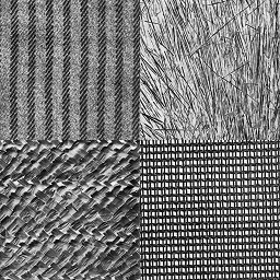
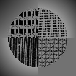
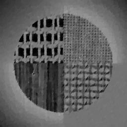
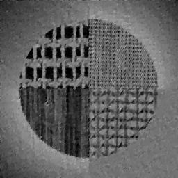
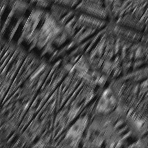
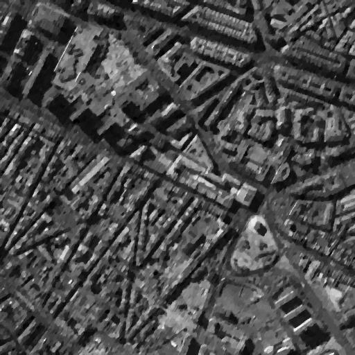
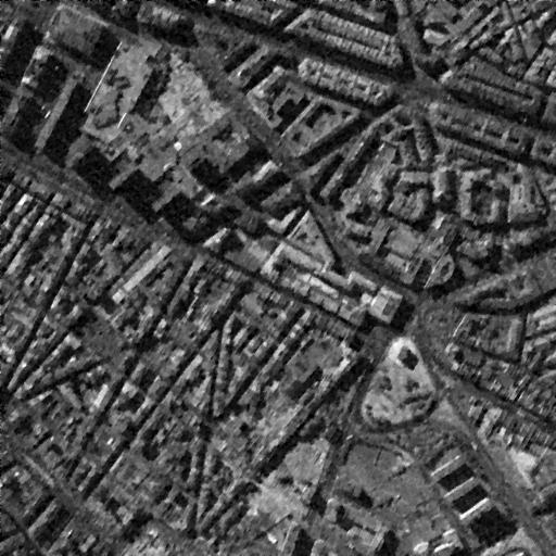
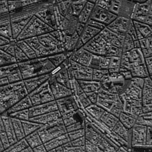
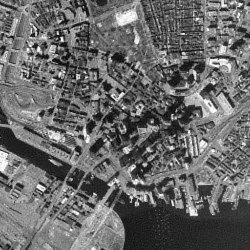
In experiments, three common types of blur kernels are considered: the motion blur kernel with angle and length , disk kernel with a radius of and average kernel. We test several noisy blurred images, distorted by Gaussian noise with a standard deviation and by blurring with one of the previously mentioned kernels, to verify the effectiveness of the proposed model. For illustration, the result for the texture1 ( pixels), texture2 ( pixels), hybrid ( pixels), satellite1( pixels), satellite2( pixels) and satellite3( pixels) are presented, see the original test images in Figure 1.


The proposed model is compared with fast total variation (FastTV) minimization [26], nonlocal total variation (NLTV) method [17, 58], nonlocal adaptive biharmonic (NLABH) regularization [51], a nonlinear fractional diffusion (NFD) model [23] and a Perona-Malik type equation regularized by the -Laplacian (PLRPM) [21]. The free parameters for FastTV, NLTV, NLABH, NFD and PLRPM are set as suggested in the reference papers. For the proposed model, while there may be more suitable parameter choices for each image, in this paper, we set , , , , , , , and throughout all experiments. For the texture1, texture2, hybrid, satellite 1, satellite 2 and satellite 3 images, we select and respectively. The parameter is chosen based on the specific image and the type of blur kernel.
| Figure 2 | Figure 3 | Figure 4 | ||||
|---|---|---|---|---|---|---|
| PSNR | SSIM | PSNR | SSIM | PSNR | SSIM | |
| FastTV | 15.17 | 0.5320 | 19.00 | 0.6887 | 21.00 | 0.7136 |
| NLTV | 16.35 | 0.6599 | 19.26 | 0.7427 | 21.14 | 0.7087 |
| NLABH | 16.11 | 0.6698 | 18.89 | 0.6710 | 20.21 | 0.4598 |
| NFD | 16.18 | 0.6738 | 19.06 | 0.6763 | 20.36 | 0.4723 |
| PLRPM | 16.30 | 0.6599 | 19.29 | 0.7068 | 21.17 | 0.6415 |
| Ours | 16.25 | 0.6745 | 19.39 | 0.6992 | 21.17 | 0.6281 |
| Figure 5 | Figure 6 | Figure 7 | ||||
|---|---|---|---|---|---|---|
| PSNR | SSIM | PSNR | SSIM | PSNR | SSIM | |
| FastTV | 23.97 | 0.8888 | 24.91 | 0.9322 | 22.41 | 0.9229 |
| NLTV | 23.87 | 0.8838 | 25.46 | 0.9387 | 22.59 | 0.9291 |
| NLABH | 22.56 | 0.8475 | 24.82 | 0.9325 | 22.00 | 0.9049 |
| NFD | 22.67 | 0.8548 | 24.77 | 0.9301 | 22.06 | 0.9059 |
| PLRPM | 24.04 | 0.8949 | 25.28 | 0.9380 | 22.55 | 0.9205 |
| Ours | 24.44 | 0.9029 | 25.47 | 0.9395 | 22.55 | 0.9212 |
In order to quantify the restoration effect, for the original image and the compared image , the restoration performance is measured in terms of the peak signal noise ratio (PSNR)
and the structural similarity index measure (SSIM)
where are two variables to stabilize the division with weak denominator, and are the local means, standard deviations and cross-covariance for image , respectively. The better quality image will have higher values of PSNR and SSIM. For a comparison of the performance quantitatively, we list the PSNR and SSIM values of the restored results in Table 1 and Table 2.
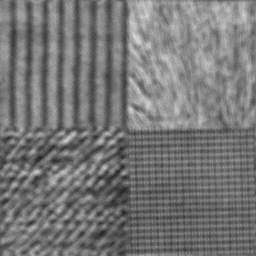
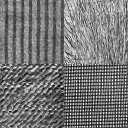
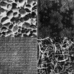
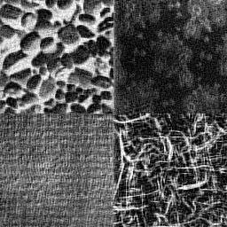
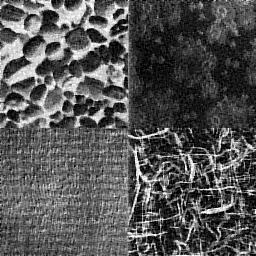
Now we report the numerical experiments of deblurring and denoising for the original test images in Figure 1. The corresponding results are shown in Figures 2-7. Firstly, the restoration results for texture1 and texture2 are shown in Figures 2 and 3. Texture1 and texture2 images are blurred by disk kernel and average kernel, respectively. For these two experiments, we select in the proposed model. We find that in Figures 2 and 3, there is minimal noise present, but the visual quality is over-smooth, with an evident loss of texture information. On the other hand, in Figures 2, 2, 3 and 3, texture details are better preserved, however, there is an increase in the noise level of the images. Compared to Figures 2, 3, 2 and 3, the restoration results of the proposed model exhibit slightly higher noise levels but retain more texture information, resulting in a better visual quality, see Figures 2 and 3.
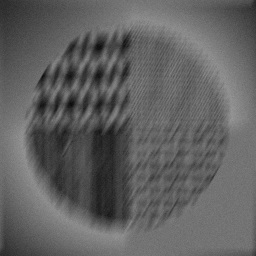
For the restoration results of the hybrid image, some new phenomena emerge, as illustrated in Figure 4. The central area of the hybrid image is rich in texture, while the surrounding area in smooth, as shown in Figure 4. The hybrid image is blurred by a motion kernel, posing a challenge for all models, see Figure 4. For this experiment, we select in the proposed model. It is observed from Figure 4 that the restoration result of FastTV contains fewer noise and artifacts in smooth areas, but it fails to preserve texture information. NLABH and NFD noticeably amplify noise in smooth regions and produce obvious artifacts, as seen in Figures 4 and 4. In the restoration results of the proposed model, noise in smooth areas is slightly more pronounced compared to NLTV and PLRPM, but texture preservation is better than PLRPM, and there are no artifacts in smooth regions as seen in the restoration results of NLTV, see Figures 4, 4, and 4.
Finally, the restoration results for three satellite images are shown in Figures 5-7. The three satellite images are respectively blurred by motion kernel, disk kernel, and average kernel, as shown in Figures 5, 6, and 7. We select in the proposed model respectively for these three experiments. Similar to the previous experiments, the restoration results of FastTV and NLTV are relatively smooth, and the noise levels in the restoration results of NLABH and NFD are increased. Overall, the methods with better visual restoration results are NLTV, PLRPM, and the proposed method. Our method slightly reduces visual quality on satellite3 due to increased noise in smooth regions, but performs best on satellite1 and satellite2, as shown in Figures 5, 6, and 7.


References
- Amann [1993] H. Amann, Nonhomogeneous Linear and Quasilinear Elliptic and Parabolic Boundary Value Problems, Vieweg+Teubner Verlag, Wiesbaden, 1993, pp. 9–126.
- Amann [1995] H. Amann, Linear and Quasilinear Parabolic Problems, Birkhäuser Basel, 1995.
- Amann [2004] H. Amann, Maximal regularity for nonautonomous evolution equations, Adv. Nonlinear Stud. 4 (2004) 417–430. https://doi.org/10.1515/ans-2004-0404.
- Amann [2005] H. Amann, Quasilinear parabolic problems via maximal regularity, Adv. Differ. Equations 10 (2005) 1081–1110. https://doi.org/10.57262/ade/1355867805.
- Amann et al. [1994] H. Amann, M. Hieber, G. Simonett, Bounded -calculus for elliptic operators, Differ. Integr. Equations 7 (1994) 613 – 653. https://doi.org/10.57262/die/1370267697.
- Bai and Feng [2007] J. Bai, X. C. Feng, Fractional-order anisotropic diffusion for image denoising, IEEE Trans. Image Process. 16 (2007) 2492–2502. https://doi.org/10.1109/TIP.2007.904971.
- Barenblatt et al. [1990] G. I. Barenblatt, V. M. Entov, V. M. Ryzhik, Theory of fluid flows through natural rocks, volume 395, Springer, 1990.
- Bertozzi and Greer [2004] A. L. Bertozzi, J. B. Greer, Low-curvature image simplifiers: Global regularity of smooth solutions and laplacian limiting schemes, Commun. Pure Appl. Math. 57 (2004) 764–790. https://doi.org/10.1002/cpa.20019.
- Boussinesq [1904] J. Boussinesq, Recherches théoriques sur l’écoulement des nappes d’eau infiltrées dans le sol et sur le débit des sources, J. Math. Pures Appl. 10 (1904) 5–78.
- Bredies et al. [2010] K. Bredies, K. Kunisch, T. Pock, Total generalized variation, SIAM J. Imag. Sci. 3 (2010) 492–526. https://doi.org/10.1137/090769521.
- Catté et al. [1992] F. Catté, P. L. Lions, J. M. Morel, T. Coll, Image selective smoothing and edge detection by nonlinear diffusion, SIAM J. Numer. Anal. 29 (1992) 182–193. https://doi.org/10.1137/0729012.
- Chan et al. [2013] R. H. Chan, A. Lanza, S. Morigi, F. Sgallari, An adaptive strategy for the restoration of textured images using fractional order regularization, Numer. Math. Theory Methods Appl. 6 (2013) 276–296. https://doi.org/doi.org/10.4208/nmtma.2013.mssvm15.
- Chiappinelli and Nugari [1995] R. Chiappinelli, R. Nugari, The nemitskii operator in hölder spaces: some necessary and sufficient conditions, J. London Math. Soc. 51 (1995) 365–372. https://doi.org/10.1112/jlms/51.2.365.
- Engel et al. [2000] K. J. Engel, R. Nagel, S. Brendle, One-parameter semigroups for linear evolution equations, Springer New York, 2000.
- Friedman [1983] A. Friedman, Partial Differential Equations of Parabolic Type, R.E. Krieger Publishing Company, 1983.
- Gilboa and Osher [2007] G. Gilboa, S. Osher, Nonlocal linear image regularization and supervised segmentation, Multiscale Model. Sim. 6 (2007) 595–630. https://doi.org/10.1137/060669358.
- Gilboa and Osher [2009] G. Gilboa, S. Osher, Nonlocal operators with applications to image processing, Multiscale Model. Sim. 7 (2009) 1005–1028. https://doi.org/10.1137/070698592.
- Guidotti [2009] P. Guidotti, A new nonlocal nonlinear diffusion of image processing, J. Differ. Equations 246 (2009) 4731–4742. https://doi.org/10.1016/j.jde.2009.03.017.
- Guidotti [2010] P. Guidotti, A new well-posed nonlinear nonlocal diffusion, Nonlinear Anal. Theory Methods Appl. 72 (2010) 4625–4637. https://doi.org/10.1016/j.na.2010.02.040.
- Guidotti [2012] P. Guidotti, A backward–forward regularization of the perona–malik equation, J. Differ. Equations 252 (2012) 3226–3244. https://doi.org/10.1016/j.jde.2011.10.022.
- Guidotti et al. [2013] P. Guidotti, Y. Kim, J. Lambers, Image restoration with a new class of forward-backward-forward diffusion equations of perona–malik type with applications to satellite image enhancement, SIAM J. Imag. Sci. 6 (2013) 1416–1444. https://doi.org/10.1137/120882895.
- Guidotti and Longo [2011] P. Guidotti, K. Longo, Well-posedness for a class of fourth order diffusions for image processing, Nonlinear Differ. Equations Appl. 18 (2011) 407–425. https://doi.org/10.1007/s00030-011-0101-x.
- Guo et al. [2019] Z. Guo, W. Yao, J. Sun, B. Wu, Nonlinear fractional diffusion model for deblurring images with textures, Inverse Probl. Imaging 13 (2019) 1161–1188. https://doi.org/10.3934/ipi.2019052.
- Hajiaboli [2009] M. R. Hajiaboli, A self-governing hybrid model for noise removal, in: T. Wada, F. Huang, S. Lin (Eds.), Advances in Image and Video Technology, Springer Berlin Heidelberg, Berlin, Heidelberg, 2009, pp. 295–305.
- Hieber and Prüss [1997] M. G. Hieber, J. Prüss, Heat kernels and maximal - estimates for parabolic evolution equations, Commun. Partial Differ. Equations 22 (1997) 1647–1669. https://doi.org/10.1080/03605309708821314.
- Huang et al. [2008] Y. Huang, M. K. Ng, Y. W. Wen, A fast total variation minimization method for image restoration, Multiscale Model. Sim. 7 (2008) 774–795. https://doi.org/10.1137/070703533.
- Karami et al. [2018] F. Karami, K. Sadik, L. Ziad, A variable exponent nonlocal -laplacian equation for image restoration, Comput. Math. Appl. 75 (2018) 534–546. https://doi.org/10.1016/j.camwa.2017.09.034.
- Kindermann et al. [2005] S. Kindermann, S. Osher, P. W. Jones, Deblurring and denoising of images by nonlocal functionals, Multiscale Model. Sim. 4 (2005) 1091–1115. https://doi.org/10.1137/050622249.
- Kunstmann and Weis [2004] P. C. Kunstmann, L. Weis, Maximal -regularity for Parabolic Equations, Fourier Multiplier Theorems and -functional Calculus, Springer Berlin Heidelbergv, Berlin, Heidelberg, 2004, pp. 65–311.
- Lunardi [1995] A. Lunardi, Analytic semigroups and optimal regularity in parabolic problems, Birkhäuser Basel, 1995.
- Majee et al. [2020] S. Majee, R. K. Ray, A. K. Majee, A gray level indicator-based regularized telegraph diffusion model: Application to image despeckling, SIAM J. Imag. Sci. 13 (2020) 844–870. https://doi.org/10.1137/19M1283033.
- Muskat [1937] M. Muskat, The flow of fluids through porous media, J. Appl. Phys. 8 (1937) 274–282. https://doi.org/10.1063/1.1710292.
- Perona and Malik [1990] P. Perona, J. Malik, Scale-space and edge detection using anisotropic diffusion, IEEE Trans. Pattern Anal. Mach. Intell. 12 (1990) 629–639. https://doi.org/10.1109/34.56205.
- Poynton [2012] C. Poynton, Digital video and HD: Algorithms and Interfaces, second edition ed., Morgan Kaufmann, 2012. URL: https://www.sciencedirect.com/book/9780123919267.
- Prüss et al. [2009] J. Prüss, G. Simonett, R. Zacher, On convergence of solutions to equilibria for quasilinear parabolic problems, J. Differ. Equations 246 (2009) 3902–3931. https://doi.org/10.1016/j.jde.2008.10.034.
- Rudin and Osher [1994] L. I. Rudin, S. Osher, Total variation based image restoration with free local constraints, in: Proceedings of 1st International Conference on Image Processing, volume 1, 1994, pp. 31–35 vol.1.
- Rudin et al. [1992] L. I. Rudin, S. Osher, E. Fatemi, Nonlinear total variation based noise removal algorithms, Physica D 60 (1992) 259–268. https://doi.org/10.1016/0167-2789(92)90242-F.
- Shan et al. [2019] X. Shan, J. Sun, Z. Guo, Multiplicative noise removal based on the smooth diffusion equation, J. Math. Imaging Vision 61 (2019) 763–779. https://doi.org/10.1007/s10851-018-00870-z.
- Shan et al. [2022] X. Shan, J. Sun, Z. Guo, W. Yao, Z. Zhou, Fractional-order diffusion model for multiplicative noise removal in texture-rich images and its fast explicit diffusion solving, BIT Numer. Math. 62 (2022) 1319–1354. https://doi.org/10.1007/s10543-022-00913-3.
- Shao et al. [2022] J. Shao, Z. Guo, W. Yao, D. Yan, B. Wu, A non-local diffusion equation for noise removal, Acta Math. Sci. 42 (2022) 1779–1808. https://doi.org/10.1007/s10473-022-0505-1.
- Shi [2021] K. Shi, Image denoising by nonlinear nonlocal diffusion equations, J. Comput. Appl. Math. 395 (2021) 113605. https://doi.org/10.1016/j.cam.2021.113605.
- Solonnikov [1965] V. A. Solonnikov, Boundary value problems of mathematical physics. Part 3. On boundary value problems for linear parabolic systems of differential equations of general form, volume 83, Russian Academy of Sciences, Steklov Mathematical Institute of Russian, 1965.
- Takeda et al. [2008] H. Takeda, S. Farsiu, P. Milanfar, Deblurring using regularized locally adaptive kernel regression, IEEE Trans. Image Process. 17 (2008) 550–563. https://doi.org/10.1109/TIP.2007.918028.
- Triebel [1978] H. Triebel, Interpolation Theory, Function Spaces, Differential Operators, North-Holland Mathematical Library, 1978.
- Tumblin and Turk [1999] J. Tumblin, G. Turk, Lcis: A boundary hierarchy for detail-preserving contrast reduction, in: Proceedings of the 26th Annual Conference on Computer Graphics and Interactive Techniques, SIGGRAPH 1999, Association for Computing Machinery, Inc, 1999, pp. 83–90. https://doi.org/10.1145/311535.311544.
- Vazquez [2006] J. L. Vazquez, The Porous Medium Equation: Mathematical Theory, Oxford University Press, 2006.
- Weickert [1997] J. Weickert, A review of nonlinear diffusion filtering, in: B. ter Haar Romeny, L. Florack, J. Koenderink, M. Viergever (Eds.), Scale-Space Theory in Computer Vision, Springer Berlin Heidelberg, Berlin, Heidelberg, 1997, pp. 1–28.
- Weickert et al. [1998] J. Weickert, B. Romeny, M. Viergever, Efficient and reliable schemes for nonlinear diffusion filtering, IEEE Trans. Image Process. 7 (1998) 398–410. https://doi.org/10.1109/83.661190.
- Welk et al. [2005] M. Welk, D. Theis, T. Brox, J. Weickert, PDE-based deconvolution with forward-backward diffusivities and diffusion tensors, in: R. Kimmel, N. A. Sochen, J. Weickert (Eds.), Scale Space and PDE Methods in Computer Vision, Springer Berlin Heidelberg, Berlin, Heidelberg, 2005, pp. 585–597.
- Wen et al. [2022] Y. Wen, J. Sun, Z. Guo, A new anisotropic fourth-order diffusion equation model based on image features for image denoising, Inverse Probl. Imaging 16 (2022) 895–924. https://doi.org/10.3934/ipi.2022004.
- Wen et al. [2023] Y. Wen, L. A. Vese, K. Shi, Z. Guo, J. Sun, Nonlocal adaptive biharmonic regularizer for image restoration, J. Math. Imaging Vision 65 (2023) 453–471. https://doi.org/10.1007/s10851-022-01129-4.
- Xu et al. [2015] M. Xu, J. Yang, D. Zhao, H. Zhao, An image-enhancement method based on variable-order fractional differential operators, Bio-Med. Mater. Eng. 26 (2015) S1325–S1333. https://doi.org/10.3233/BME-151430.
- Yao et al. [2019] W. Yao, Z. Guo, J. Sun, B. Wu, H. Gao, Multiplicative noise removal for texture images based on adaptive anisotropic fractional diffusion equations, SIAM J. Imag. Sci. 12 (2019) 839–873. https://doi.org/10.1137/18M1187192.
- Yin et al. [2016] X. Yin, S. Zhou, M. A. Siddique, Fractional nonlinear anisotropic diffusion with -laplace variation method for image restoration, Multimedia Tools Appl. 75 (2016) 4505–4526. https://doi.org/10.1007/s11042-015-2488-6.
- You and Kaveh [2000] Y. L. You, M. Kaveh, Fourth-order partial differential equations for noise removal, IEEE Trans. Image Process. 9 (2000) 1723–1730. https://doi.org/10.1109/83.869184.
- Zel’Dovich and Raizer [2002] Y. B. Zel’Dovich, Y. P. Raizer, Physics of shock waves and high-temperature hydrodynamic phenomena, Courier Corporation, 2002.
- Zhang and Chen [2015] J. Zhang, K. Chen, A total fractional-order variation model for image restoration with nonhomogeneous boundary conditions and its numerical solution, SIAM J. Imag. Sci. 8 (2015) 2487–2518. https://doi.org/10.1137/14097121X.
- Zhang et al. [2010] X. Zhang, M. Burger, X. Bresson, S. Osher, Bregmanized nonlocal regularization for deconvolution and sparse reconstruction, SIAM J. Imag. Sci. 3 (2010) 253–276. https://doi.org/10.1137/090746379.
- Zhou et al. [2015] Z. Zhou, Z. Guo, G. Dong, J. Sun, D. Zhang, B. Wu, A doubly degenerate diffusion model based on the gray level indicator for multiplicative noise removal, IEEE Trans. Image Process. 24 (2015) 249–260. https://doi.org/10.1109/TIP.2014.2376185.
- Zhou et al. [2018] Z. Zhou, Z. Guo, D. Zhang, B. Wu, A nonlinear diffusion equation-based model for ultrasound speckle noise removal, J. Nonlinear Sci. 28 (2018) 443–470. https://doi.org/10.1007/s00332-017-9414-1.