Flat sub-Lorentzian structures on Martinet distribution

Abstract

Two flat sub-Lorentzian problems on the Martinet distribution are studied. For the first one, the attainable set has a nontrivial intersection with the Martinet plane, but for the second one it does not. Attainable sets, optimal trajectories, sub-Lorentzian distances and spheres are described.

Keywords: Sub-Lorentzian geometry, geometric control theory, Martinet distribution, sub-Lorentzian length maximizers, sub-Lorentzian distance, sub-Lorentzian sphere

1 Introduction

Sub-Riemannian geometry studies manifolds $M$ in which the distance between points $q_{0},q_{1}\in M$ is the infimum of the lengths of all curves tangent to a given distribution and connecting $q_{0}$ to $q_{1}$ [1, 2]. In more detail, for the distribution $\Delta\subset TM$ in each space $\Delta_{q}\subset T_{q}M$ the scalar product $g_{q}$ is given, and the length of the curve $q(t)$, $t\in[0,t_{1}]$, tangent $\Delta$, is measured as in Riemannian geometry: $l(q(\cdot))=\int_{0}^{t_{1}}\sqrt{g(\dot{q}(t))}dt$.

If in each space $\Delta_{q}\subset T_{q}M$ we define a non-degenerate quadratic form $g_{q}$ of index 1, then a sub-Lorentzian structure $(\Delta,g)$ will be defined on the manifold $M$. Here the natural problem is to find the longest relative to $g$ curve connecting given points. Sub-Lorentzian geometry strives to build a theory similar to the rich theory of sub-Riemannian geometry, and is at the beginning of its development. The foundations of sub-Lorentzian geometry were laid in the works of M. Grochowski [3, 4, 5, 6, 7, 8], see also [9, 11, 12, 10].

Just as in sub-Riemannian geometry, the simplest sub-Lorentzian problem arises on the Heisenberg group; it has been fully studied [7, 13]. The next most important model of sub-Riemannian geometry after the Heisenberg group arises on the Martinet distribution [1, 17, 2, 18].

The purpose of this work is to consider two flat sub-Lorentzian problems on the Martinet distribution: to describe the optimal synthesis, distance and spheres. In the first problem, the future cone has a non-trivial intersection with the tangent space to the Martinet surface; in the second case this intersection is trivial. Accordingly, in the first case the sub-Lorentzian geometry is much more complicated, see Conclusion.

The structure of this work is as follows. In Section 2 we recall the basic facts of sub-Lorentzian geometry required in the sequel.

The main Sections 3 and 4 are devoted respectively to the first and the second flat sub-Lorentzian problems on the Martinet distribution; they have identical structure as follows. First we find an invariant set (a candidate attainable set) via the geometric statement of Pontryagin maximum principle. Then we describe explicitly abnormal and normal extremal trajectories; normal trajectories are parametrized by the sub-Lorentzian exponential mapping. We prove diffeomorphic properties of the exponential mapping via Hadamard’s global diffeomorphism theorem. On this basis we show that the above-mentioned invariant set is indeed the attainable set, and prove a theorem on existence of optimal trajectories. After that we study optimality of extremal trajectories, which yields an optimal synthesis. We complete our study by describing main properties of sub-Lorentzian distance and sphere.

In the concluding Sec. 5 we discuss the results obtained for two problems.

2 Sub-Lorentzian geometry

A sub-Lorentzian structure on a smooth manifold $M$ is a pair $(\Delta,g)$ consisting of a vector distribution $\Delta\subset TM$ and a Lorentzian metric $g$ on $\Delta$, i.e., a nondegenerate quadratic form $g$ of index 1. Let us recall some basic definitions of sub-Lorentzian geometry. A vector $v\in T_{q}M$, $q\in M$, is called horizontal if $v\in\Delta_{q}$. A horizontal vector $v$ is called:

• timelike if $g(v)<0$,

• spacelike if $g(v)>0$ or $v=0$,

• lightlike if $g(v)=0$ and $v\neq 0$,

• nonspacelike if $g(v)\leq 0$.

A Lipschitzian curve in $M$ is called timelike if it has timelike velocity vector a.e.; spacelike, lightlike and nonspacelike curves are defined similarly.

A time orientation $X$ is an arbitrary timelike vector field in $M$. A nonspacelike vector $v\in\Delta_{q}$ is future directed if $g(v,X(q))<0$, and past directed if $g(v,X(q))>0$.

A future directed timelike curve $q(t)$, $t\in[0,t_{1}]$, is called arclength parametrized if $g(\dot{q}(t),\dot{q}(t))\equiv-1$. Any future directed timelike curve can be parametrized by arclength, similarly to the arclength parametrization of a horizontal curve in sub-Riemannian geometry.

The length of a nonspacelike curve $\gamma\in\operatorname{Lip}\nolimits([0,t_{1}],M)$ is

$$l(\gamma)=\int_{0}^{t_{1}}|g(\dot{\gamma},\dot{\gamma})|^{1/2}dt.$$

For points $q_{1},q_{2}\in M$ denote by $\Omega_{q_{1}q_{2}}$ the set of all future directed nonspacelike curves in $M$ that connect $q_{1}$ to $q_{2}$. In the case $\Omega_{q_{1}q_{2}}\neq\emptyset$ denote the sub-Lorentzian distance from the point $q_{1}$ to the point $q_{2}$ as

$$d(q_{1},q_{2})=\sup\{l(\gamma)\mid\gamma\in\Omega_{q_{1}q_{2}}\}.$$ (2.1)

And if $\Omega_{q_{1}q_{2}}=\emptyset$ then $d(q_{1},q_{2}):=0$. A future directed nonspacelike curve $\gamma$ is called a sub-Lorentzian length maximizer if it realizes the supremum in $(\ref{d})$ between its endpoints $\gamma(0)=q_{1}$, $\gamma(t_{1})=q_{2}$.

The causal future of a point $q_{0}\in M$ is the set $J^{+}(q_{0})$ of points $q_{1}\in M$ for which there exists a future directed nonspacelike curve $\gamma$ that connects $q_{0}$ and $q_{1}$.

Let $q_{0}\in M$, $q_{1}\in J^{+}(q_{0})$. The search for sub-Lorentzian length maximizers that connect $q_{0}$ with $q_{1}$ reduces to the search for future directed nonspacelike curves $\gamma$ that solve the problem

$$l(\gamma)\to\max,\qquad\gamma(0)=q_{0},\quad\gamma(t_{1})=q_{1}.$$ (2.2)

A set of vector fields $X_{1},\dots,X_{k}\in\operatorname{Vec}\nolimits(M)$ is an orthonormal frame for a sub-Lorentzian structure $(\Delta,g)$ if for all $q\in M$

$$\Delta_{q}=\operatorname{span}\nolimits(X_{1}(q),\dots,X_{k}(q)),$$

$$g_{q}(X_{1},X_{1})=-1,\qquad g_{q}(X_{i},X_{i})=1,\quad i=2,\dots,k,$$

$$g_{q}(X_{i},X_{j})=0,\quad i\neq j.$$

Assume that time orientation is defined by a timelike vector field $X\in\operatorname{Vec}\nolimits(M)$ for which $g(X,X_{1})<0$ (e.g., $X=X_{1}$). Then the sub-Lorentzian problem for the sub-Lorentzian structure with the orthonormal frame $X_{1},\dots,X_{k}$ is stated as the following optimal control problem:

$$\dot{q}=\sum_{i=1}^{k}u_{i}X_{i}(q),\qquad q\in M,$$

$$u\in U=\left\{(u_{1},\dots,u_{k})\in{\mathbb{R}}^{k}\mid u_{1}\geq\sqrt{u_{2}^{2}+\dots+u_{k}^{2}}\right\},$$

$$q(0)=q_{0},\qquad q(t_{1})=q_{1},$$

$$l(q(\cdot))=\int_{0}^{t_{1}}\sqrt{u_{1}^{2}-u_{2}^{2}-\dots-u_{k}^{2}}\,dt\to\max.$$

Remark 1.

The sub-Lorentzian length is preserved under monotone Lipschitzian time reparametrizations $t(s)$, $s\in[0,s_{1}]$. Thus if $q(t)$, $t\in[0,t_{1}]$, is a sub-Lorentzian length maximizer, then so is any its reparametrization $q(t(s))$, $s\in[0,s_{1}]$.

In this paper we choose primarily the following parametrization of trajectories: the arclength parametrization ($u_{1}^{2}-u_{2}^{2}-\cdots-u_{k}^{2}\equiv 1$) for timelike trajectories, and the parametrization with $u_{1}(t)\equiv 1$ for future directed lightlike trajectories.

3 The first problem

Let $M={\mathbb{R}}^{3}_{x,y,z}$, $X_{1}=\frac{\partial\,}{\partial\,x}$, $X_{2}=\frac{\partial\,}{\partial\,y}+\frac{x^{2}}{2}\frac{\partial\,}{\partial\,z}$. The distribution $\Delta=\operatorname{span}\nolimits(X_{1},X_{2})$ is called the Martinet distribution [1, 17, 2, 18]. The plane $\Pi=\{x=0\}$ is called the Martinet surface. The distribution $\Delta$ has growth vector $(2,3)$ outside of $\Pi$, and growth vector $(2,2,3)$ on $\Pi$. This distribution is called flat since the Lie algebra generated by the vector fields $X_{1}$, $X_{2}$ is a Carnot algebra (Engel algebra), the nonzero Lie brackets of these vector fields are: $[X_{1},X_{2}]=xX_{3}$, $[X_{1},xX_{3}]=X_{3}:=\frac{\partial\,}{\partial\,z}$.

In this section we study a sub-Lorentzian problem in which the interior of the future cone intersects nontrivially with the tangent space to the Martinet plane $\Pi$.

3.1 Problem statement

The first flat sub-Lorentzian problem on the Martinet distribution is stated as the following optimal control problem [14, 16]:

$$\dot{q}=u_{1}X_{1}+u_{2}X_{2},\qquad q\in M,$$ (3.1)

$$u=(u_{1},u_{2})\in U_{1}=\{u_{2}\geq|u_{1}|\},$$ (3.2)

$$q(0)=q_{0}=(0,0,0),\qquad q(t_{1})=q_{1},$$ (3.3)

$$l=\int_{0}^{t_{1}}\sqrt{u_{2}^{2}-u_{1}^{2}}dt\to\max,$$ (3.4)

see Fig. 1.

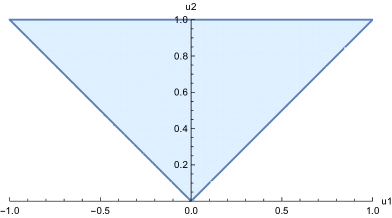
Figure 1: The set $U_{1}$

3.2 Invariant set

In this subsection we compute an invariant set $\mathcal{B}_{1}$ of system $(\ref{pr11})$, $(\ref{pr12})$. Later, in Th. 3, we prove that $\mathcal{B}_{1}$ is the attainable set $\mathcal{A}_{1}$ of system $(\ref{pr11})$, $(\ref{pr12})$ from the point $q_{0}$ for arbitrary nonnegative time (the causal future of the point $q_{0}$).

By the geometric statement of Pontryagin maximum principle (PMP) for free time ([14], Th. 12.8), if a trajectory $q(t)$ corresponding to a control $u(t)$, $t\in[0,t_{1}]$, satisfies the inclusion $q(t_{1})\in\partial\mathcal{A}_{1}$, then there exists a Lipschitzian curve $\lambda_{t}\in T^{*}_{q(t)}M$, $\lambda_{t}\neq 0$, $t\in[0,t_{1}]$, such that

$$\dot{\lambda}_{t}=\vec{h}_{u(t)}(\lambda_{t}),$$ (3.5)

$$h_{u(t)}(\lambda_{t})=\max_{u\in U_{1}}h_{u}(\lambda_{t}),$$ (3.6)

$$h_{u(t)}(\lambda_{t})=0$$

for almost all $t\in[0,t_{1}]$. Here $h_{u}(\lambda)=u_{1}h_{1}(\lambda)+u_{2}h_{2}(\lambda)$, $h_{i}(\lambda)=\langle\lambda,X_{i}(\pi(\lambda))\rangle$, $i=1,2$, and $\pi\,:\,T^{*}M\to M$ is the canonical projection of the cotangent bundle, $\pi(\lambda)=q$, $\lambda\in T^{*}_{q}M$. Moreover, $\vec{h}_{u}(\lambda)$ is the Hamiltonian vector field on the cotangent bundle $T^{*}M$ with the Hamoltonian $h_{u}(\lambda)$.

We have $[X_{1},X_{1}]=xX_{3}$, $X_{3}=\frac{\partial\,}{\partial\,z}$, and if we denote $h_{3}(\lambda)=\langle\lambda,X_{3}(\pi(\lambda))\rangle$, then the Hamiltonian system $(\ref{Ham01})$ reads

$$\dot{h}_{1}=-u_{2}xh_{3},\quad\dot{h}_{2}=u_{1}xh_{3},\quad\dot{h}_{3}=0,\quad\dot{q}=u_{1}X_{1}+u_{2}X_{2}.$$

The maximality condition $(\ref{max1})$ implies that up to reparameterization there can be two cases:

• $u(t)=(\pm 1,1)$,

• $u(t)=(0,1)$, $x(t)=0$.

Take any $0\leq t_{1}\leq t_{2}$ and compute trajectories with one switching corresponding to the following controls:

1) Let

$$u(t)=\begin{cases}(1,1),&t\in[0,t_{1}],\\ (-1,1),&t\in[t_{1},t_{2}].\end{cases}$$

Then $x(t)=t$, $y(t)=t$, $z(t)=t^{3}/6$ for $t\in[0,t_{1}]$, $x(t)=2t_{1}-t$, $y(t)=t$, $z(t)=t_{1}^{3}/6+(4t_{1}^{2}(t-t_{1})-2t_{1}(t^{2}-t_{1}^{2})+(t^{3}-t_{1}^{3})/3)$ for $t\in[t_{1},t_{2}]$, thus $x(t_{2})=2t_{1}-t_{2}$, $y(t_{2})=t_{2}$, $z(t_{2})=-t_{1}^{3}+2t_{1}^{2}t_{2}-t_{1}t_{2}^{2}+t_{2}^{3}/6$. Thus the endpoint $q(t_{2})$ satisfies the equality

$$z=(-3x^{3}+3x^{2}y+3xy^{2}+y^{3})/24.$$ (3.7)

2) Let

$$u(t)=\begin{cases}(-1,1),&t\in[0,t_{1}],\\ (1,1),&t\in[t_{1},t_{2}].\end{cases}$$

Then $x(t)=-t$, $y(t)=t$, $z(t)=t^{3}/6$ for $t\in[0,t_{1}]$, $x(t)=t-2t_{1}$, $y(t)=t$, $z(t)=((t^{3}-t_{1}^{3})/3-2t_{1}(t^{2}-t_{1}^{2})+4t_{1}^{2}(t-t_{1}))/2$ for $t\in[t_{1},t_{2}]$, thus $x(t_{2})=t_{2}-2t_{1}$, $y(t_{2})=t_{2}$, $z(t_{2})=-t_{1}^{3}+2t_{1}^{2}t_{2}-t_{1}t_{2}^{2}+t_{2}^{3}/6$. Thus the endpoint $q(t_{2})$ satisfies the equality

$$z=(3x^{3}+3x^{2}y-3xy^{2}+y^{3})/24.$$ (3.8)

3) Let

$$u(t)=\begin{cases}(0,1),&t\in[0,t_{1}],\\ (1,1),&t\in[t_{1},t_{2}].\end{cases}$$

Then $x(t)=0$, $y(t)=t$, $z(t)=0$ for $t\in[0,t_{1}]$, $x(t)=t-t_{1}$, $y(t)=t$, $z(t)=(t-t_{1})^{3}/6$ for $t\in[t_{1},t_{2}]$, thus $x(t_{2})=t_{2}-t_{1}$, $y(t_{2})=t_{2}$, $z(t_{2})=(t_{2}-t_{1})^{3}/6$. Thus the endpoint $q(t_{2})$ satisfies the equality

$$z=x^{3}/6.$$ (3.9)

4) Finally, let

$$u(t)=\begin{cases}(0,1),&t\in[0,t_{1}],\\ (-1,1),&t\in[t_{1},t_{2}].\end{cases}$$

Then $x(t)=0$, $y(t)=t$, $z(t)=0$ for $t\in[0,t_{1}]$, $x(t)=t_{1}-t$, $y(t)=t$, $z(t)=(t-t_{1})^{3}/6$ for $t\in[t_{1},t_{2}]$, thus $x(t_{2})=t_{1}-t_{2}$, $y(t_{2})=t_{2}$, $z(t_{2})=(t_{2}-t_{1})^{3}/6$. Thus the endpoint $q(t_{2})$ satisfies the equality

$$z=-x^{3}/6.$$ (3.10)

Consider the surfaces $S_{1}$–$S_{4}$ given by Eqs. $(\ref{zS1})$–$(\ref{zS4})$ respectively,

$$S_{1}\ :\ z=(-3x^{3}+3x^{2}y+3xy^{2}+y^{3})/24,\qquad x\geq 0,$$

$$S_{2}\ :\ z=(3x^{3}+3x^{2}y-3xy^{2}+y^{3})/24,\qquad x\leq 0,$$

$$S_{3}\ :\ z=x^{3}/6,\qquad x\geq 0,$$

$$S_{4}\ :\ z=-x^{3}/6,\qquad x\leq 0.$$

Introduce the homogeneous coordinates on the set $\{y\neq 0\}$ induced by the one-parameter group of dilations $(\ref{dilat})$:

$$\xi=\frac{x}{y},\qquad\eta=\frac{24z-3x^{2}y-y^{3}}{24y^{3}}.$$ (3.11)

Then the surfaces $S_{1}$–$S_{4}$ are given as follows:

$$S_{1}\ :\ \eta=\frac{\xi(1-\xi^{2})}{8}=:\varphi_{1}(\xi),\qquad \xi\in[0,1],$$

$$S_{2}\ :\ \eta=\frac{\xi(\xi^{2}-1)}{8}=:\varphi_{2}(\xi)=\varphi_{1}(-\xi),\qquad \xi\in[-1,0],$$

$$S_{3}\ :\ \eta=\frac{\xi^{3}}{6}-\frac{3\xi^{2}+1}{24}=:\varphi_{3}(\xi),\qquad \xi\in[0,1],$$

$$S_{4}\ :\ \eta=-\frac{\xi^{3}}{6}-\frac{3\xi^{2}+1}{24}=:\varphi_{4}(\xi)=\varphi_{3}(-\xi),\qquad \xi\in[-1,0].$$

The surface $\cup_{i=1}^{4}S_{i}$ bounds a domain

$$\mathcal{B}_{1}=\begin{cases}\varphi_{3}(\xi)\leq\eta\leq\varphi_{1}(\xi),\qquad&0\leq\xi\leq 1,\\ \varphi_{4}(\xi)\leq\eta\leq\varphi_{2}(\xi),\qquad&-1\leq\xi\leq 0,\end{cases}$$

see Figs. 3–5.

Figure 2: The boundary of $\mathcal{B}_{1}$

Figure 3: The boundary of $\mathcal{B}_{1}$

Figure 4: The boundary of $\mathcal{B}_{1}$

Figure 5: The boundary of $\mathcal{B}_{1}$ projected to $(\xi,\eta)$

Recall that $\mathcal{A}_{1}$ is the attainable set of system $(\ref{pr11})$, $(\ref{pr12})$ from the point $q_{0}$ for arbitrary nonnegative time (the causal future of the point $q_{0}$).

Proposition 1.

The set $\mathcal{B}_{1}$ is an invariant domain of system $(\ref{pr11})$, $(\ref{pr12})$. Moreover, $\mathcal{A}_{1}\subset B_{1}$.

Proof.

Direct computation shows that on each of the surfaces $S_{1}$–$S_{4}$ the vector field $u_{1}X_{1}+u_{2}X_{2}$, $(u_{1},u_{2})\in U_{1}$, is directed inside the domain $\mathcal{B}_{1}$. Since $q_{0}\in\mathcal{B}_{1}$, then $\mathcal{A}_{1}\subset\mathcal{B}_{1}$. ∎

We show in Th. 3 that $\mathcal{A}_{1}=\mathcal{B}_{1}$.

3.3 Extremal trajectories

Introduce the family of Hamiltonians of Pontryagin maximum principle (PMP) [15, 14] $h_{u}^{\nu}(\lambda)=u_{1}h_{1}(\lambda)+u_{2}h_{2}(\lambda)-\nu\sqrt{u_{2}^{2}-u_{1}^{2}}$, where $\lambda\in T^{*}M$, $(u_{1},u_{2})\in U_{1}$, $\nu\in\{-1,0\}$. By PMP (Th. 12.10 [14]), if $q(t)$, $t\in[0,t_{1}]$, is an optimal trajectory in problem $(\ref{pr11})$–$(\ref{pr14})$, then there exist a Lipschitzian curve $\lambda_{t}\in T_{q(t)}^{*}M$, $t\in[0,t_{1}]$, and a number $\nu\in\{-1,0\}$ such that

$$\dot{\lambda}_{t}=\vec{h}^{\nu}_{u(t)}(\lambda_{t}),$$

$$h^{\nu}_{u(t)}(\lambda_{t})=\max_{v\in U_{1}}h_{v}(\lambda_{t}),$$

$$(\lambda_{t},\nu)\neq(0,0)$$

for almost all $t\in[0,t_{1}]$.

3.3.1 Abnormal extremal trajectories

If $\nu=0$, then the control satisfies, up to reparameterization, the conditions

• $u(t)=(\pm 1,1)$,

• $u(t)=(0,1)$, $x(t)=0$,

and has up to one switching. These trajectories were computed in Subsec. 3.2, they form the boundary of the candidate attainable set $\mathcal{B}_{1}$.

Remark 2.

Abnormal trajectories starting from an arc on the plane $\Pi$ change their causal type: first they are timelike (when belong to $\Pi$), then lightlike. The remaining extremal trajectories preserve the causal type.

3.3.2 Normal extremals

If $\nu=-1$, then extremals satisfy the Hamiltonian system with the Hamiltonian $H=(h_{1}^{2}-h_{2}^{2})/2$, $h_{2}<-|h_{1}|$:

$$\dot{h}_{1}=h_{2}h_{3}x,\quad\dot{h}_{2}=h_{1}h_{3}x,\quad\dot{h}_{3}=0,\quad\dot{x}=h_{1},\quad\dot{y}=-h_{2},\quad\dot{z}=-h_{2}x^{2}/2.$$ (3.12)

We can choose arclength parameterization on normal extremal trajectories and thus assume that $H\equiv-1/2$. In the coordinates $h_{1}=\sinh\psi$, $h_{2}=-\cosh\psi$, $h_{3}=c$; $\psi,c\in{\mathbb{R}}$, the Hamiltonian system $(\ref{Ham0})$ reads

$$\dot{\psi}=-cx,\qquad\dot{c}=0,$$ (3.13)

$$\dot{x}=\sinh\psi,\qquad\dot{y}=\cosh\psi,\qquad\dot{z}=\cosh\psi x^{2}/2.$$ (3.14)

This system has an energy integral $E=cx^{2}/2+\cosh\psi\in[1,+\infty)$.

Remark 3.

The normal Hamiltonian system $(\ref{Ham1})$, $(\ref{Ham2})$ has a discrete symmetry — reflection

$$(\psi,c,x,y,z)\mapsto(-\psi,c,-x,y,z),$$ (3.15)

and a one-parameter family of symmetries — dilations

$$(t,\psi,c,x,y,z)\mapsto(\alpha t,\psi,c/\alpha^{2},\alpha x,\alpha y,\alpha^{3}z),\qquad\alpha>0.$$ (3.16)

Moreover, the parallel translations

$$(x,y,z)\mapsto(x,y+a,z+b),\qquad a,b\in{\mathbb{R}},$$ (3.17)

are symmetries of the problem since their generating vector fields $\frac{\partial\,}{\partial\,y}$, $\frac{\partial\,}{\partial\,z}$ commute with the vector fields $X_{1}$, $X_{2}$ of the orthonormal frame.

1) If $c=0$, then

$$\psi\equiv\psi_{0},\qquad x=t\sinh\psi_{0},\qquad y=t\cosh\psi_{0},\qquad z=t^{3}/6\cosh\psi_{0}\sinh^{2}\psi_{0}.$$ (3.18)

If $c\neq 0$, then extremal trajectories in the Martinet flat case are obtained by a linear change of variables from extremal trajectories of a left-invariant sub-Lorentzian problem on the Engel group [19].

2) Let $c=l^{2}>0$.

2.1) If $\psi_{0}=0$, then $x=z\equiv 0$, $y=t$.

2.2) Let $\operatorname{sgn}\nolimits\psi_{0}=\pm 1$, $E=\cosh\psi_{0}>1$, $k=\sqrt{\frac{E-1}{E+1}}\in(0,1)$, $k^{\prime}=\sqrt{1-k^{2}}$, $m=lk^{\prime}$, $\mbox{\ae}=1/k^{\prime}$, $\tau=\mbox{\ae}lt$. Then

$$x=\pm\frac{2k}{m}\operatorname{sn}\nolimits\tau,$$

$$y=\frac{1}{m}(2\operatorname{E}\nolimits(\tau)-k^{\prime 2}\tau),$$

$$z=-\frac{2}{3m^{3}}\left(k^{\prime 2}\tau+2k^{2}\operatorname{sn}\nolimits\tau\operatorname{cn}\nolimits\tau\operatorname{dn}\nolimits\tau-(1+k^{2})\operatorname{E}\nolimits(\tau)\right),$$

where $\operatorname{sn}\nolimits\tau$, $\operatorname{cn}\nolimits\tau$, $\operatorname{dn}\nolimits\tau$ are Jacobi’s elliptic functions with modulus $k$, and $\operatorname{E}\nolimits(\tau)=\int_{0}^{\tau}\operatorname{dn}\nolimits^{2}tdt$ is Jacobi’s epsilon function [20, 21]. See Figs. 7–9.

3) Let $c=-l^{2}<0$.

3.1) If $\psi_{0}=0$, then $x=z\equiv 0$, $y=t$.

3.2) Let $\operatorname{sgn}\nolimits\psi_{0}=\pm 1$, $E=\cosh\psi_{0}>1$, $k=\sqrt{\frac{2}{1+E}}\in(0,1)$, $k^{\prime}=\sqrt{1-k^{2}}$, $m=kl$, $\tau=lt/k$. Then

$$x=\pm\frac{2k^{\prime}}{m}\frac{\operatorname{sn}\nolimits\tau}{\operatorname{cn}\nolimits\tau},$$

$$y=\frac{1}{m}\left((2-k^{2})\tau+2\frac{\operatorname{dn}\nolimits\tau\operatorname{sn}\nolimits\tau}{\operatorname{cn}\nolimits\tau}-2\operatorname{E}\nolimits(\tau)\right),$$

$$z=-\frac{2}{3m^{3}}\left(2k^{\prime 2}\tau+(k^{2}-2)\operatorname{E}\nolimits(\tau)+(k^{2}+(k^{2}-2)\operatorname{sn}\nolimits^{2}\tau)\frac{\operatorname{dn}\nolimits\tau\operatorname{sn}\nolimits\tau}{\operatorname{cn}\nolimits^{3}\tau}\right),$$

$$\tau\in[0,K(k)),$$

where $K(k)$ is the complete elliptic integral of the second kind [20, 21].

Figure 6: The curve $(x(t),y(t))$ for $c=1$, $\psi_{0}=0$

Figure 7: The curve $(x(t),y(t))$ for $c=1$, $\psi_{0}=1$

Figure 8: The curve $(x(t),y(t))$ for $c=1$, $\psi_{0}=2$

Figure 9: The curve $(x(t),y(t))$ for $c=1$, $\psi_{0}=4$

3.4 Exponential mapping

Introduce the exponential mapping

$$\operatorname{Exp}\nolimits\,:\,N\to M,\qquad\operatorname{Exp}\nolimits(\lambda,t)=\pi\circ e^{t\vec{H}}(\lambda),$$

$$N=\{(\lambda,t)\in C\times{\mathbb{R}}_{+}\mid t\in(0,+\infty)\text{ for }c\geq 0;\ \ t\in(0,+kK/l)\text{ for }c<0\},$$

$$C=T_{q_{0}}^{*}M\cap\{H=-1/2,\ h_{2}<0\}.$$

Formulas of Subsec. 3.3.2 give an explicit parametrization of the exponential mapping.

In this subsection we describe diffeomorphic properties of the exponential mapping via the classical Hadamard’s theorem on global diffeomorphism:

Theorem 1 ([22]).

Let $F\,:\,X\to Y$ be a smooth mapping of smooth manifolds, $\dim X=\dim Y$. Suppose that the following conditions hold:

• $X$ and $Y$ are connected,

• $Y$ is simply connected,

• $F$ is nondegenerate,

• $F$ is proper (i.e., for any compact set $K\subset Y$, the preimage $F^{-1}(K)\subset X$ is compact).

Then $F$ is a diffeomorphism.

Consider the following stratification in the image of the exponential mapping:

$$\operatorname{int}\nolimits\mathcal{B}_{1}=\cup_{i=0}^{6}M_{i},$$

$$M_{0}\ :\ x=0,\qquad-1/24<\eta<0,$$

$$M_{1}\ :\ x>0,\qquad\varphi_{5}(\xi)<\eta<\varphi_{1}(\xi),$$

$$M_{2}\ :\ x<0,\qquad\varphi_{5}(\xi)<\eta<\varphi_{2}(\xi),$$

$$M_{3}\ :\ x>0,\qquad\varphi_{3}(\xi)<\eta<\varphi_{5}(\xi),$$

$$M_{4}\ :\ x<0,\qquad\varphi_{2}(\xi)<\eta<\varphi_{4}(\xi),$$

$$M_{5}\ :\ x>0,\qquad\eta=\varphi_{5}(\xi),$$

$$M_{6}\ :\ x<0,\qquad\eta=\varphi_{5}(\xi),$$

$$\varphi_{5}(\xi)=(\xi^{2}-1)/24,$$

see Fig. 10.

Figure 10: Stratification in the image of $\operatorname{Exp}\nolimits$

And define the following stratification of the subset

$$\widetilde{N}=\{(\lambda,t)\in N\mid t\in(0,2K/(\mbox{\ae}l))\text{ for }c>0;\ t\in(0,+\infty)\text{ for }c=0;\ t\in(0,kK/l)\text{ for }c<0\}$$

in the preimage of the exponential mapping:

$$\widetilde{N}=\cup_{i=1}^{6}\widetilde{N}_{i},$$

$$\widetilde{N}_{1}\ :\ c>0,\qquad\psi_{0}>0,\qquad\tau\in(0,2K),$$

$$\widetilde{N}_{2}\ :\ c>0,\qquad\psi_{0}<0,\qquad\tau\in(0,2K),$$

$$\widetilde{N}_{3}\ :\ c<0,\qquad\psi_{0}>0,\qquad\tau\in(0,K),$$

$$\widetilde{N}_{4}\ :\ c<0,\qquad\psi_{0}<0,\qquad\tau\in(0,K),$$

$$\widetilde{N}_{5}\ :\ c=0,\qquad\psi_{0}>0,$$

$$\widetilde{N}_{6}\ :\ c=0,\qquad\psi_{0}<0.$$

Proposition 2.

There holds the inclusion $\operatorname{Exp}\nolimits(\widetilde{N}_{1})\subset M_{1}$. Moreover, the mapping $\operatorname{Exp}\nolimits\,:\,\widetilde{N}_{1}\to M_{1}$ is a real-analytic diffeomorphism.

Proof.

a) Let us show that $\operatorname{Exp}\nolimits(\widetilde{N}_{1})\subset M_{1}$.

Let $(\lambda,t)\in\widetilde{N}_{1}$. We have to prove that $(\xi^{2}-1)/24<\eta<\xi(1-\xi^{2})/8$, i.e.,

$$(x^{2}-y^{2})y\underset{1)}{<}24z-3x^{2}y-y^{3}\underset{2)}{<}3x(y^{2}-x^{2}).$$

Inequality $1)$ is rewritten as

$$6z>x^{2}y.$$ (3.19)

Differentiating this inequality by virtue of ODEs $(\ref{Ham2})$, we get

$$x\cosh\psi>y\sinh\psi.$$ (3.20)

Differentiating once more, we get

$$x\sinh\psi>y\cosh\psi.$$ (3.21)

Since $\cosh\psi>\sinh\psi>0$, we have $y>x$, and inequality $(\ref{1.3})$ is proved. Since the both sides of this inequality vanish at $t=0$, inequality $(\ref{1.2})$ is proved as well. Similarly, inequality $(\ref{1.1})$ is proved, thus inequality $1)$ follows.

Now we prove similarly inequality $2)$: it is equivalent to

$$24z<y^{3}+3x^{2}y+3xy^{2}-3x^{3}.$$

Differentiating, we get

$$3x^{2}<y^{2}+2xy,$$

which holds since $y>x$. Returning back, we prove inequality $2)$.

So the inclusion $\operatorname{Exp}\nolimits(\widetilde{N}_{1})\subset M_{1}$ is proved.

b) We show that the mapping $\operatorname{Exp}\nolimits\,:\,\widetilde{N}_{1}\to M_{1}$ is nondegenerate, i.e., the Jacobian $J=\frac{\partial(x,y,z)}{\partial(c,\psi,t)}$ does not vanish on $\widetilde{N}_{1}$. Direct computation of this Jacobian gives

$$J=f\cdot\frac{\partial(x,y,z)}{\partial(m,\tau,k)}=f\cdot\frac{9(1-k^{2})k^{2}m^{6}}{32}J_{1},\qquad f\neq 0,$$

$$J_{1}=J_{0}+o(1),\qquad k\to 0,$$

$$J_{0}=\cos(3\tau)+(8\tau^{2}-1)\cos\tau-4\tau\sin\tau.$$

Since

$$\left(\frac{J_{0}}{\sin\tau}\right)^{\prime}=-\frac{2(2\tau-\sin 2\tau)^{2}}{\sin^{2}\tau}<0,\qquad\tau\in(0,\pi),$$

thus $J_{0}(\tau)<0$, $\tau\in(0,\pi]$.

Moreover,

$$\left.J_{1}\right|_{\tau=2K}=12(1-k^{2})g(k),$$

$$g(k)=E^{2}(k)-2E(k)K(k)+(1-k^{2})K^{2}(k).$$ (3.22)

We have $g(k)=g_{1}(k)g_{2}(k)$, $g_{1}(k)=E(k)-(1+k)K(k)$, $g_{2}(k)=E(k)-(1-k)K(k)$. Since $g_{1}^{\prime}(k)=\frac{E(k)}{k-1}<0$, then $g_{1}(k)<0$ for $k\in(0,1)$. Similarly, since $g_{2}^{\prime}(k)=\frac{E(k)}{k+1}>0$, then $g_{2}(k)>0$ for $k\in(0,1)$. Thus $g(k)<0$ and $\left.J_{2}\right|_{\tau=2K}<0$ for $k\in(0,1)$.

By homotopy invariance of the Maslov index (the number of conjugate points on an extremal) [24], we have $J(\tau)<0$ for $\tau\in(0,2K]$. Thus the mapping $\operatorname{Exp}\nolimits\,:\,\widetilde{N}_{1}\to M_{1}$ is nondegenerate.

c) We show that this mapping is proper. In other words, we prove that if $\widetilde{N}_{1}\ni(m,k,\tau)\to\partial\widetilde{N}_{1}$, then $q=\operatorname{Exp}\nolimits(m,k,\tau)\to\partial M_{1}$.

1) Let $\tau\to 0$.

1.1) If $m\geq\varepsilon>0$, then $x\to 0$.

1.2) Let $m\to 0$.

1.2.1) If $\tau/m\to 0$, then $x\to 0$.

1.2.2) Let $\tau/m\geq\varepsilon>0$.

1.2.2.1) If $\tau/m\to\infty$, then $y\to\infty$.

1.2.2.2) If $\tau/m\leq K$, then $\varphi_{1}\to 0$.

2) Let $\tau\geq\varepsilon>0$.

2.1) Let $\operatorname{am}\nolimits\tau\to\pi$, where $\operatorname{am}\nolimits\tau$ is the Jacobi amplitude of modulus $k$.

2.1.1) If $m\geq\delta>0$, then $x\to 0$.

2.1.2) If $m\to 0$, then $y\to\infty$.

2.2) Let $\operatorname{am}\nolimits\tau\leq\pi-\gamma<\pi$.

2.2.1) Let $m\to 0$.

2.2.1.1) If $k\geq\sigma>0$, then $x\to\infty$.

2.2.1.2) Let $k\to 0$.

2.2.1.2.1) If $k/m\to 0$, then $x\to 0$.

2.2.1.2.2) If $k/m\to\infty$, then $x\to\infty$.

2.2.1.2.3) If $\alpha\leq k/m\leq\beta$, then $y\to\infty$.

2.2.2) Let $m\geq\delta>0$.

2.2.2.1) If $m\to\infty$, then $x\to 0$.

2.2.2.2) Let $m\leq\alpha$.

2.2.2.2.1) If $k\to 0$, then $x\to 0$.

2.2.2.2.2) If $k\to 1$, then $\varphi_{1}\to 0$.

Summing up, the mapping $\operatorname{Exp}\nolimits\,:\,\widetilde{N}_{1}\to M_{1}$ is proper.

Since $\widetilde{N}_{1}$ and $M_{1}$ are connected and simply connected, this mapping is a diffeomorphism by Th. 1. ∎

Proposition 3.

There holds the inclusion $\operatorname{Exp}\nolimits(\widetilde{N}_{3})\subset M_{3}$. Moreover, the mapping $\operatorname{Exp}\nolimits\,:\,\widetilde{N}_{3}\to M_{3}$ is a real-analytic diffeomorphism.

Proof.

Similarly to Propos. 2. ∎

Proposition 4.

There hold the inclusions $\operatorname{Exp}\nolimits(\widetilde{N}_{2})\subset M_{2}$ and $\operatorname{Exp}\nolimits(\widetilde{N}_{4})\subset M_{4}$. Moreover, the mappings $\operatorname{Exp}\nolimits\,:\,\widetilde{N}_{2}\to M_{2}$ and $\operatorname{Exp}\nolimits\,:\,\widetilde{N}_{4}\to M_{4}$ are real-analytic diffeomorphisms.

Proof.

Follows from Propositions 2 and 3 via reflection $(\ref{refl})$. ∎

Proposition 5.

There holds the inclusions $\operatorname{Exp}\nolimits(\widetilde{N}_{5})\subset M_{5}$, $\operatorname{Exp}\nolimits(\widetilde{N}_{6})\subset M_{6}$. Moreover, the mappings $\operatorname{Exp}\nolimits\,:\,\widetilde{N}_{5}\to M_{5}$, $\operatorname{Exp}\nolimits\,:\,\widetilde{N}_{6}\to M_{6}$ are real-analytic diffeomorphisms.

Proof.

Follows from the parametrization $(\ref{c=0})$ of the exponential mapping $\left.\operatorname{Exp}\nolimits\right|_{\widetilde{N}5}$. ∎

Introduce the following subsets in the preimage of the exponential mapping:

$$N_{0}^{\pm}=\{(\lambda,t)\in N\mid c>0,\ \operatorname{sgn}\nolimits\psi_{0}=\pm 1,\ t=2K/(\mbox{\ae}l)\}.$$

Proposition 6.

There hold the inclusions $\operatorname{Exp}\nolimits(N_{0}^{\pm})\subset M_{0}$. Moreover, the mappings $\operatorname{Exp}\nolimits\,:\,N_{0}^{\pm}\to M_{0}$ are real-analytic diffeomorphisms.

Proof.

In view of the reflection $(\ref{refl})$, it suffices to consider only the set $N_{0}^{+}$. And in view of the dilations $(\ref{dilat})$, it is enough to consider only the case $c=1$.

If $c=1$, $\psi_{0}>0$, $t=2K/(\mbox{\ae}l)=2K/k^{\prime}$, then

$$x=0,$$

$$y=k^{\prime}(4E(k)-2k^{\prime 2}K(k)),$$

$$z=\frac{4}{3}k^{\prime 3}((1+k^{2})E(k)-k^{\prime 2}K(k)),$$

$$\xi=0,$$

$$\eta=-\frac{1}{24}+\frac{(1+k^{2})E(k)-(1-k^{2})K(k)}{6(2E(k)-(1-k^{2})K(k))^{3}}=:\eta_{1}(k).$$

We have $\lim_{k\to 0}\eta_{1}(k)=-1/24$, $\lim_{k\to 1}\eta_{1}(k)=0$ and $\eta_{1}^{\prime}(k)=-\frac{(1-k^{2})g(k)}{2k(2E(k)-(1-k^{2})K(k))^{4}}$, where the function $g(k)$ is given by $(\ref{g(k)})$. We showed in the proof of Propos. 2 that $g(k)<0$, $k\in(0,1)$, thus $\eta_{1}\,:\,(0,1)\to(-1/24,0)$ is a strictly increasing diffeomorphism.

Thus $\operatorname{Exp}\nolimits(N_{0}^{+})\subset M_{0}$ and $\operatorname{Exp}\nolimits\,:\,N_{0}^{+}\to M_{0}$ is a diffeomorphism. ∎

Denote

$$N_{+}=\widetilde{N}_{1}\cup\widetilde{N}_{3}\cup N_{5},$$

$$N_{-}=\widetilde{N}_{2}\cup\widetilde{N}_{4}\cup N_{6},$$

$$M_{+}=M_{1}\cup M_{3}\cup M_{5}=(\operatorname{int}\nolimits\mathcal{B}_{1})\cap\{x>0\},$$

$$M_{-}=M_{2}\cup M_{4}\cup M_{6}=(\operatorname{int}\nolimits\mathcal{B}_{1})\cap\{x<0\}.$$

Theorem 2.

There hold the inclusions $\operatorname{Exp}\nolimits(N_{\pm})\subset M_{\pm}$. Moreover, the mappings $\operatorname{Exp}\nolimits\,:\,N_{\pm}\to M_{\pm}$ are real-analytic diffeomorphisms.

Proof.

By virtue of the reflection $(\ref{refl})$, it suffices to consider only the domain $N_{+}$.

The inclusion $\operatorname{Exp}\nolimits(N_{+})\subset M_{+}$ follows from Propositions 2, 3, 5.

The mappings $\left.\operatorname{Exp}\nolimits\right|_{\widetilde{N}_{1}}$ and $\left.\operatorname{Exp}\nolimits\right|_{\widetilde{N}_{3}}$ are nondegenerate by Propositions 2 and 3 respectively. Since $\widetilde{N}_{5}\subset\operatorname{cl}\nolimits(\widetilde{N}_{1})$ and $\left.\operatorname{Exp}\nolimits\right|_{\widetilde{N}_{1}}$ is nondegenerate, then it follows by homotopy invariance of the Maslov index that the mapping $\operatorname{Exp}\nolimits\,:\,N_{+}\to M_{+}$ is also nondegenerate at the set $N_{5}$. Summing up, $\left.\operatorname{Exp}\nolimits\right|_{N_{+}}$ is nondegenerate.

Similarly to the proof of Propos. 2 it follows that the mapping $\operatorname{Exp}\nolimits\,:\,N_{+}\to M_{+}$ is proper.

Then Theorem 1 implies that this mapping is a diffeomorphism. ∎

Proposition 7.

The mapping $\operatorname{Exp}\nolimits\,:\,N\to M$ is a local diffeomorphism at points of $N_{0}^{\pm}$.

Proof.

By virtue of the reflection $(\ref{refl})$, we can consider only the case $N_{0}^{+}$.

But $N_{0}^{+}\subset\operatorname{cl}\nolimits(\widetilde{N}_{1})$ and $\operatorname{Exp}\nolimits\,:\,\widetilde{N}_{1}\to M$ is nondegenerate. Then by homotopy invariance of the Maslov index the mapping $\operatorname{Exp}\nolimits\,:\,N\to M$ is a local diffeomorphism at points of $N_{0}^{+}$. ∎

3.5 Attainable sets and existence of optimal trajectories

Theorem 3.

We have $\mathcal{A}_{1}=\mathcal{B}_{1}$.

Proof.

By virtue of Propos. 1, it remains to prove the inclusion $\mathcal{A}_{1}\supset\mathcal{B}_{1}$. But Theorem 2 and Propos. 6 imply that $\operatorname{Exp}\nolimits(N_{+}\cup N_{-}\cup N_{0}^{+})\supset M_{+}\cup M_{-}\cup M_{0}=\operatorname{int}\nolimits\mathcal{B}_{1}$. Thus $\mathcal{A}_{1}\supset\operatorname{int}\nolimits\mathcal{B}_{1}$.

Further, each point of $\partial\mathcal{B}_{1}$ is reachable from $q_{0}$ by an abnormal trajectory, thus $\mathcal{A}_{1}\supset\partial\mathcal{B}_{1}$.

Summing up, $\mathcal{A}_{1}\supset\mathcal{B}_{1}$, and the equality $\mathcal{A}_{1}=\mathcal{B}_{1}$ follows. ∎

Recall that $J^{+}(q)$ is the causal future of a point $q\in M$, i.e., the attainable set from $q$ for arbitrary nonnegative time. Similarly, $J^{-}(q)$ is the causal past of $q$, i.e., the set of points attainable from $q$ for arbitrary nonpositive time. Notice that $\mathcal{A}_{1}=J^{+}({q_{0}})$.

Corollary 1.

Let $q=(0,y_{0},z_{0})\in M$. Then

$$J^{+}(q)=\begin{cases}\varphi_{3}(\xi_{0})\leq\eta_{0}\leq\varphi_{1}(\xi_{0}),\qquad&0\leq\xi_{0}\leq 1,\qquad y\geq y_{0},\\ \varphi_{4}(\xi_{0})\leq\eta_{0}\leq\varphi_{2}(\xi_{0}),\qquad&-1\leq\xi_{0}\leq 0,\qquad y\geq y_{0},\end{cases}$$

$$\xi_{0}=\frac{x}{y-y_{0}},\qquad\eta_{0}=\frac{24(z-z_{0})-3x^{2}(y-y_{0})-(y-y_{0})^{3}}{24(y-y_{0})^{3}},$$

$$J^{-}(q)=\begin{cases}\varphi_{3}(\xi_{1})\leq\eta_{1}\leq\varphi_{1}(\xi_{1}),\qquad&0\leq\xi_{1}\leq 1,\qquad y\leq y_{0},\\ \varphi_{4}(\xi_{1})\leq\eta_{1}\leq\varphi_{2}(\xi_{1}),\qquad&-1\leq\xi_{1}\leq 0,\qquad y\leq y_{0},\end{cases}$$

$$\xi_{1}=-\xi_{0},\qquad\eta_{1}=\eta_{0}.$$

Proof.

The expression for $J^{+}(q)$ follows from the expression for $J^{+}({q_{0}})=\mathcal{A}_{1}$ via the translation $(\ref{paral})$. And the expression for $J^{-}(q)$ follows by time inversion. ∎

Theorem 4.

Let points $q_{0},q_{1}\in M$ satisfy the inclusion $q_{1}\in J^{+}({q_{0}})$. Then there exists an optimal trajectory in problem $(\ref{pr11})$–$(\ref{pr14})$.

Proof.

By Theorem 2 and Remark 2 [23], the following conditions are sufficient for existence of an optimal trajectory connecting $q_{0}$ and $q_{1}$:

• $q_{1}\in J^{+}({q_{0}})$,

• There exists a compact $K\subset M$ such that $J^{+}({q_{0}})\cap J^{-}_{q_{1}}\subset K$,

• $T(q_{0},q_{1})<+\infty$,

where $T(q_{0},q_{1})$ is the supremum of time required to reach $q_{1}$ from $q_{0}$ for a trajectory of system $(\ref{pr11})$ reparametrized so that $u_{1}\equiv 1$.

Condition (1) holds by assumption of this theorem.

Condition (3) holds since if $u\equiv 1$ then $\dot{y}\equiv 1$, thus $T(q_{0},q_{1})=y_{1}-y_{0}<+\infty$.

Now we prove condition (2). It is easy to see from Cor. 1 that

$$\cup_{q\in\Pi}J^{+}(q)=\cup_{q\in\Pi}J^{-}(q)=M.$$

Thus there exist $p_{0},p_{1}\in\Pi$ such that $p_{0}\in J^{+}({q_{0}})$, $q_{1}\in J^{-}({p_{1}})$. Thus $J^{+}({q_{0}})\subset J^{+}({p_{0}})$, $J^{-}({q_{1}})\subset J^{-}({p_{1}})$, so $J^{+}({q_{0}})\cap J^{-}({q_{1}})\subset J^{+}({p_{0}})\cap J^{-}({p_{1}})$. It is easy to see from Cor. 1 that the set $K:=J^{+}({p_{0}})\cap J^{-}({p_{1}})$ is compact. So condition (2) above holds, and this theorem is proved. ∎

3.6 Optimality of extremal trajectories

Proposition 8.

Let $\lambda=(\psi_{0},c)\in C$, $c>0$, $\psi_{0}\neq 0$, and let $t_{1}>2K/({\text{\em\ae}}l)$. Then the extremal trajectory $q(t)=\operatorname{Exp}\nolimits(\lambda,t)$, $t\in[0,t_{1}]$, is not optimal.

Proof.

By virtue of the reflection $(\ref{refl})$, we can assume that $\psi_{0}>0$. By contradiction, suppose that $q(t)$, $t\in[0,t_{1}]$, is optimal.

Let $\widetilde{\lambda}=(-\psi_{0},c)\in C$, $\widetilde{q}(t)=\operatorname{Exp}\nolimits(\widetilde{\lambda},t)$, $t\in[0,t_{1}]$. Denote $\bar{t}=2K/(\mbox{\ae}l)$, then $q(\bar{t})=\widetilde{q}(\bar{t})$ and $l(\left.q(\cdot)\right|_{[0,\bar{t}]})=l(\left.\widetilde{q}(\cdot)\right|_{[0,\bar{t}]})$, i.e., the trajectories $q(\cdot)$ and $\widetilde{q}(\cdot)$ have a Maxwell point at $t=\bar{t}$ [25]. Now consider the trajectory

$$\widehat{q}(t)=\begin{cases}\widetilde{q}(t),\qquad&t\in[0,\bar{t}],\\ q(t),\qquad&t\in[\bar{t},t_{1}].\end{cases}$$

Since $l(\left.\widehat{q}(\cdot)\right|_{[0,t_{1}]})=l(\left.q(\cdot)\right|_{[0,t_{1}]})$, then the trajectory $\widehat{q}(t)$, $t\in[0,t_{1}]$, is optimal. But $\widehat{q}(t)$ has a corner point at $t=\bar{t}$, which is not possible for normal trajectories. Thus $\widehat{q}(t)$ is abnormal, so its support belongs to $\partial\mathcal{A}_{1}$. But this is impossible since the support of the normal trajectory $q(t)$ belongs to $\operatorname{int}\nolimits\mathcal{A}_{1}$. A contradiction obtained completes the proof. ∎

Define the following function:

$$\mathbf{t}\,:\,C\to(0,+\infty],\qquad\lambda=(\psi_{0},c)\in C,$$

$$c=0\quad\Rightarrow\quad\mathbf{t}(\lambda)=+\infty,$$

$$c\neq 0,\ \psi_{0}=0\quad\Rightarrow\quad\mathbf{t}(\lambda)=+\infty,$$

$$c>0,\ \psi_{0}\neq 0\quad\Rightarrow\quad\mathbf{t}(\lambda)=\frac{2kK}{l},$$

$$c<0,\ \psi_{0}\neq 0\quad\Rightarrow\quad\mathbf{t}(\lambda)=\frac{kK}{l}.$$

We prove (see Cor. 2) that $\mathbf{t}(\lambda)$ is the cut time for an extremal trajectory $\operatorname{Exp}\nolimits(\lambda,t)$:

$$\mathbf{t}(\lambda)=t_{\operatorname{cut}\nolimits}(\lambda):=\sup\{t_{1}>0\mid\operatorname{Exp}\nolimits(\lambda,t)\text{ is optimal for }t\in[0,t_{1}]\}.$$

Theorem 5.

Let $\lambda\in C$, $t_{1}\in(0,\mathbf{t}(\lambda))$. Then the trajectory $q(t)=\operatorname{Exp}\nolimits(\lambda,t)$, $t\in[0,t_{1}]$, is optimal.

Proof.

By Theorem 4, there exists an optimal trajectory connecting $q_{0}$ and $q_{1}:=q(t_{1})$. Since $q_{1}\in\operatorname{int}\nolimits\mathcal{A}_{1}$, this trajectory is a normal extremal trajectory. Since $q_{1}\in M_{+}\cup M_{-}$, by Theorem 2 there exists a unique arclength parametrized normal extremal trajectory connecting $q_{0}$ and $q_{1}$, so it coincides with $q(t)$. ∎

Theorem 6.

Let $\lambda=(\psi_{0},c)\in C$, $c>0$, $\psi_{0}\neq 0$, $t_{1}=\mathbf{t}(\lambda)$. Then the trajectory $q(t)=\operatorname{Exp}\nolimits(\lambda,t)$, $t\in[0,t_{1}]$, is optimal.

Proof.

Similarly to Th. 5 with the only distinction that now there are exactly two optimal trajectories corresponding to the covectors $(\pm\psi_{0},c)\in C$, these trajectories are symmetric by virtue of the reflection $(\ref{refl})$. ∎

Proposition 8 and Theorems 5, 6 imply the following.

Corollary 2.

For any $\lambda\in C$ we have $t_{\operatorname{cut}\nolimits}(\lambda)=\mathbf{t}(\lambda)$.

Proposition 9.

Any abnormal extremal trajectory is optimal.

Proof.

Abnormal extremal trajectories are exactly trajectories belonging to the boundary of the attainable set $\mathcal{A}_{1}$. If $q(t)$, $t\in[0,t_{1}]$, is an abnormal trajectory, then, up to reparametrization, the corresponding control has the following form:

$$1)\ u(t)=\begin{cases}(\pm 1,1),&t\in[0,\tau_{1}],\\ (\mp 1,1),&t\in[\tau_{1},t_{1}],\end{cases}\quad\tau_{1}\in[0,t_{1}],\text{ or}$$

$$2)\ u(t)=\begin{cases}(0,1),&t\in[0,\tau_{1}],\\ (\pm 1,1),&t\in[\tau_{1},t_{1}],\end{cases}\quad\tau_{1}\in[0,t_{1}].$$

In the case 1) we have $l(q(\cdot))=0$. If $\widetilde{q}(t)$, $t\in[0,\tilde{t}_{1}]$, is a trajectory such that $\widetilde{q}(\tilde{t}_{1})=q(t_{1})$, then, up to reparametrization, $\widetilde{q}(t)\equiv q(t)$, thus $q(t)$ is optimal.

In the case 2) we have $l(q(\cdot))=\tau_{1}$, and a similar argument shows that $q(t)$ is optimal. ∎

Theorems 5, 6 and Propos. 9 yield the following description of the optimal synthesis.

Theorem 7.

• Let $q_{1}\in(\operatorname{int}\nolimits\mathcal{A}_{1})\setminus\Pi$. Then there exists a unique optimal trajectory $\operatorname{Exp}\nolimits(\lambda,t)$, $t\in[0,t_{1}]$, where $(\lambda,t_{1})=\operatorname{Exp}\nolimits^{-1}(q_{1})$.

• Let $q_{1}\in(\operatorname{int}\nolimits\mathcal{A}_{1})\cap\Pi$. Then there exist exactly two optimal trajectories $\operatorname{Exp}\nolimits(\lambda_{i},t)$, $t\in[0,t_{1}]$, $i=1,2$, where $\{(\lambda_{1},t_{1}),(\lambda_{2},t_{1})\}=\operatorname{Exp}\nolimits^{-1}(q_{1})$.

• Let $q_{1}=(x_{1},y_{1},z_{1})\in S_{1}\cup S_{1}$, $\operatorname{sgn}\nolimits x_{1}=\pm 1$. Then there exists a unique optimal trajectory

  $$q(t)=\begin{cases}e^{t(\pm X_{1}+X_{2})}(q_{0}),\qquad&t\in[0,\tau_{1}],\\ e^{(t-\tau_{1})(\mp X_{1}+X_{2})}\circ e^{\tau_{1}(\pm X_{1}+X_{2})}(q_{0}),\qquad&t\in[\tau_{1},t_{1}],\end{cases}$$

  $\tau_{1}=(y_{1}\pm x_{1})/2$, $t_{1}=y_{1}$.

• Let $q_{1}=(x_{1},y_{1},z_{1})\in S_{3}\cup S_{4}$, $\operatorname{sgn}\nolimits x_{1}=\pm 1$. Then there exists a unique optimal trajectory

  $$q(t)=\begin{cases}e^{tX_{2}}(q_{0}),\qquad&t\in[0,\tau_{1}],\\ e^{(t-\tau_{1})(\pm X_{1}+X_{2})}\circ e^{\tau_{1}X_{2}}(q_{0}),\qquad&t\in[\tau_{1},t_{1}],\end{cases}$$

  $\tau_{1}=y_{1}\pm x_{1}$, $t_{1}=y_{1}$.

• Let $q_{1}=(0,y_{1},0)$, $y_{1}>0$. Then there exists a unique optimal trajectory $q(t)=e^{tX_{2}}(q_{0})$, $t\in[0,t_{1}]$, $t_{1}=y_{1}$.

• Let $q_{1}=(0,y_{1},z_{1})$, $z_{1}=y_{1}^{3}/24>0$. Then there exist exactly two optimal trajectories

  $$q^{1}(t)=\begin{cases}e^{t(X_{1}+X_{2})}(q_{0}),\qquad&t\in[0,\tau_{1}],\\ e^{(t-\tau_{1})(-X_{1}+X_{2})}\circ e^{\tau_{1}(X_{1}+X_{2})}(q_{0}),\qquad&t\in[\tau_{1},t_{1}],\end{cases}$$

  $$q^{2}(t)=\begin{cases}e^{t(-X_{1}+X_{2})}(q_{0}),\qquad&t\in[0,\tau_{1}],\\ e^{(t-\tau_{1})(X_{1}+X_{2})}\circ e^{\tau_{1}(-X_{1}+X_{2})}(q_{0}),\qquad&t\in[\tau_{1},t_{1}],\end{cases}$$

  $\tau_{1}=t_{1}/2$, $t_{1}=y_{1}$.

• Let $q_{1}=(x_{1},y_{1},z_{1})$, $\operatorname{sgn}\nolimits x_{1}=\pm 1$, $y_{1}=\pm x_{1}$, $z_{1}=y_{1}^{3}/6$. Then there exists a unique optimal trajectory $q(t)=e^{t(\pm X_{1}+X_{2})}(q_{0})$, $t\in[0,t_{1}]$, $t_{1}=y_{1}$.

Remark 4.

In Theorem 7 existence of exactly one (two) optimal trajectories is understood up to reparametrization.

3.7 Sub-Lorentzian distance

In this subsection we study the function $d(q):=d(q_{0},q)$, $q\in M$.

Theorem 8.

• The distance $d$ is real-analytic on $(\operatorname{int}\nolimits\mathcal{A}_{1})\setminus\Pi$ and continuous on $\operatorname{int}\nolimits\mathcal{A}_{1}$.

• The distance $d$ has discontinuity of the first kind at each point of $S_{3}\cup S_{4}$.

• The restriction $\left.d\right|_{\Pi}$ is real-analytic on the set $\{x=0,\ z\in(0,y^{3}/24),\ y>0\}$ and discontinuous of the first kind on the set $\{x=0,\ z=y^{3}/24,\ y>0\}$.

• The distance $d$ is homogeneous of order $1$ w.r.t. dilations $(\ref{dilat})$:

  $$d(\delta_{\alpha}(q))=\alpha\delta(q),\qquad\delta_{\alpha}(x,y,z)=(\alpha x,\alpha y,\alpha^{3}z),\qquad\alpha>0,\quad q=(x,y,z)\in M.$$

Proof.

(1) Follows from Th. 2 and Propos. 7.

(2) Take any $q_{1}=(x_{1},y_{1},z_{1})\in S_{3}\cup S_{4}$, then $d(q_{1})=y_{1}>0$ by item (4) of Th. 7. On the other hand, $q_{1}\in\partial\mathcal{A}_{1}$, thus there are points $q\in M\setminus\mathcal{A}_{1}$ arbitrarily close to $q_{1}$. Since $d(q)=0$, the distance $d$ has discontinuity of the first kind at $q_{1}$.

(3) The restriction $\left.d\right|_{\Pi}$ is real-analytic on the set $\{x=0,\ z\in(0,y^{3}/24),\ y>0\}$ by Propos. 7.

Let $q_{1}=(x_{1},y_{1},z_{1})\in\mathcal{A}_{1}$, $x_{1}=z_{1}=0$, $y_{1}>0$. Then $q_{1}\in\partial\mathcal{A}_{1}$, and the distance $d$ has discontinuity of the first kind at $q_{1}$ similarly to item (2).

(4) is obvious in view of symmetry $(\ref{dilat})$. ∎

Let $q=(0,y,z)\in\Pi$, then $d(q)=y^{3}d(0,1,z/y^{3})=y^{3}d(0,1,\eta+1/24)$ since $\left.\eta\right|_{\Pi}=z/y^{3}-1/24$. We plot the function $\eta\mapsto d(0,1,\eta+1/24)$ in Fig. 11.

Figure 11: Plot of $\eta\mapsto d(0,1,\eta+1/24)$

3.8 Sub-Lorentzian sphere

By virtue of dilations $(\ref{dilat})$, the Lorentzian spheres

$$S(R)=\{q\in M\mid d(q)=R\},\qquad R>0,$$

satisfy the relation $S(R)=\delta_{R}(S(1))$, thus we describe only the unit sphere $S:=S(1)$.

Theorem 9.

• The set $S\setminus(\Pi\cup\partial\mathcal{A}_{1})$ is a real-analytic manifold.

• The sphere $S$ is nonsmooth and Lipschitzian at points of $S\cap\Pi$.

• The intersection $S\cap\Pi$ is defined parametrically for $k\in[0,1)$:

  $$y=\frac{4E(k)-2(1-k^{2})K(k)}{2(1-k^{2})K(k)}=1+k^{2}+O(k^{4}),\qquad k\to 0,$$

  $$z=\frac{2(1-k^{2})K(k)-2(1+k^{2})E(k)}{12(1-k^{2})^{3}K^{3}(k)}=\frac{k^{2}}{\pi^{2}}+O(k^{4}),\qquad k\to 0.$$

  In particular, the intersection $S\cap\Pi$ is semi-analytic.

Proof.

(1) Follows from Th. 2.

(2) The hemi-spheres $S_{\pm}=S\cap\{\pm x\geq 0\}$ have at points of $S\cap\Pi$ the normal vectors $n_{\pm}=\pm(g(k),*,*)$, where the function $g(k)$ is given by $(\ref{g(k)})$ and is negative for $k\in(0,1)$. So the sphere $S$ has a transverse self-intersection at points of $S\cap\Pi$. .

(3) The parametrization of $S\cap\Pi$ is obtained from the parametrization of the exponential mapping in the case 2.2 of Subsec. 3.3.2 for $\tau=2K$, $t=1$. ∎

Remark 5.

One of the most important results of the paper [17] is non-subanalyticity of the sub-Riemannian sphere in the Martinet flat case. Its proof relies on non-semianalitycity of the intersection of the sub-Riemannian sphere with the Martinet surface. Item (3) of the preceding theorem states that such an intersection is semi-analytic in the sub-Lorentzian case. We leave the question of subanalyticity of the sub-Lorentzian sphere in the first flat problem on the Martinet distribution open since we cannot conclude on sub-analitycity (or its lack) at points of the boundary of the sphere $S$.

Denote $S_{n}=S\cap\operatorname{int}\nolimits\mathcal{A}_{1}$, $S_{a}=S\cap\partial\mathcal{A}_{1}$.

Remark 6.

The set $S_{n}$ (resp. $S_{a}$) is filled with the endpoints of optimal normal (resp. abnormal) trajectories of length $1$ starting at $q_{0}$.

Lemma 1.

We have $\operatorname{cl}\nolimits(S_{n})\supset S_{a}$.

Proof.

Take any point $q\in S_{a}$ and choose any neighbourhood $q\in O\subset M$. By Proposition 8.1 [3], the distance $d$ is upper semicontinuous on $\mathcal{A}_{1}$, thus there exists a point $q_{-}\in O\cap\operatorname{int}\nolimits\mathcal{A}_{1}$ such that $d(q_{-})\leq d(q)=1$. Further, for small $t>0$ there exists a point

$$q_{+}=e^{t(u_{1}X_{1}+u_{2}X_{2})}(q)\in O\cap\operatorname{int}\nolimits\mathcal{A}_{1},\qquad(u_{1},u_{2})\in U_{1}.$$

Then $d(q_{+})\geq 1$. Since $O\cap\operatorname{int}\nolimits\mathcal{A}_{1}$ is arcwise connected and $\left.d\right|_{\operatorname{int}\nolimits\mathcal{A}_{1}}$ is continuous, there exists a point $\bar{q}\in O\cap\operatorname{int}\nolimits\mathcal{A}_{1}$ such that $d(\bar{q})=1$. Then $\bar{q}\in S_{n}\cap O$. So $\operatorname{cl}\nolimits(S_{n})\supset S_{a}$. ∎

Proposition 10.

The sphere $S$ is homeomorphic to the closed half-plane ${\mathbb{R}}^{2}_{+}:=\{(a,b)\in{\mathbb{R}}^{2}\mid b\geq 0\}$.

Proof.

Denote the group of dilations $(\ref{dilat})$ as $G=\{\delta_{\alpha}\mid\alpha>0\}$ and consider the projection

$$p\,:\,\overset{\circ}{M}\to\overset{\circ}{M}/G,\qquad\overset{\circ}{M}=M\setminus\{q_{0}\}.$$ (3.23)

If $y\neq 0$ (which is the case on $S$), then projection $(\ref{p})$ is given in coordinates as

$$p\ :\ q=(x,y,z)\mapsto\sigma=(\xi,\eta),$$

where $\xi$, $\eta$ are defined in $(\ref{xieta})$. The mapping $(\ref{p})$ is smooth.

The image of the sphere $S$ under the action of the projection $p$ is given as follows:

$$p(S)\ :\ \begin{cases}\varphi_{3}(\xi)\leq\eta<\varphi_{1}(\xi),&0<\xi<1,\\ \varphi_{4}(\xi)\leq\eta<\varphi_{2}(\xi),&-1<\xi<0,\end{cases}$$

see Fig. 19. It is obvious that $p(S)$ is homeomorphic to ${\mathbb{R}}^{2}_{+}$. Let us show that $p\,:\,S\to p(S)$ is a homeomorphism.

First, the mapping $p\,:\,S\to p(S)$ is a bijection since the sphere $S$ intersects with each orbit of $G$ at not more than one point.

Second, the mapping $p\,:\,S\to p(S)$ is continuous as a restriction of a smooth mapping $(\ref{p})$.

It remains to prove that the inverse mapping $p^{-1}\,:\,p(S)\to S$ is continuous. Continuity of $\left.p^{-1}\right|_{p(S_{n})}$ and $\left.p^{-1}\right|_{p(S_{a})}$ is obvious. Let

$$p(S_{n})\ni\sigma_{k}\underset{k\to\infty}{\to}\bar{\sigma}\in p(S_{a}),$$

we show that $p^{-1}(\sigma_{k})=:q_{k}\underset{k\to\infty}{\to}\bar{q}:=p^{-1}(\bar{\sigma})$. It follows from Propos. 3 that $q_{k}\underset{k\to\infty}{\to}\widehat{q}\in S_{a}$, where $p(\widehat{q})=\bar{\sigma}$. Since orbits of $G$ are one-dimensional, it remains to prove that $d(\widehat{q})=1$.

By Lemma 1, there exists a sequence $S_{n}\ni\widetilde{q}_{k}\underset{k\to\infty}{\to}\bar{q}$. Thus $\widetilde{\sigma}_{k}:=p(\widetilde{q}_{k})\underset{k\to\infty}{\to}\bar{\sigma}$. Denote by $\rho$ and $\widehat{\rho}$ the Euclidean distances in $M$ and $\overset{\circ}{M}/G$ respectively. Then $\widehat{\rho}(\sigma_{k},\widetilde{\sigma}_{k})\underset{k\to\infty}{\to}0$, thus ${\rho}(q_{k},\widetilde{q}_{k})\underset{k\to\infty}{\to}0$, whence $\widehat{q}=\bar{q}$.

Thus $p\,:\,S\to p(S)$ is a homeomorphism, and $S\simeq{\mathbb{R}}^{2}_{+}$. ∎

Corollary 3.

• The sphere $S$ is a topological manifold with boundary $S_{a}$, homeomorphic to the closed half-plane ${\mathbb{R}}^{2}_{+}$.

• The sphere $S$ is a stratified space with real-analytic strata $S_{n}^{\pm}:=S_{n}\cap\{x\gtrless 0\}$, $S_{n}^{0}:=S\cap\Pi$, $S_{a}^{\pm}:=S_{a}\cap\{x\gtrless 0\}$, $S_{a}^{0}:=S_{a}\cap\Pi=\{(0,1,0)\}$. Wherein there are diffeomorphisms $S_{n}^{\pm}\to{\mathbb{R}}^{2}$; $S_{n}^{0},S_{a}^{\pm}\to{\mathbb{R}}$.

• Under a homeomorphic embedding of the sphere $S$ into the half-plane ${\mathbb{R}}^{2}_{+}=\{(a,b)\in{\mathbb{R}}^{2}\mid b\geq 0\}$ the indicated strata are mapped as follows: $S_{n}^{\pm}\to\{a\gtrless 0,b>0\}$, $S_{n}^{0}\to\{a=0,b>0\}$, $S_{a}^{\pm}\to\{a\gtrless 0,b=0\}$, $S_{a}^{0}\to\{a=b=0\}$.

See Fig. 19.

Remark 7.

There is a numerical evidence that the sphere $S$ is a piecewise smooth manifold with boundary, with a stratification shown in Fig. 19.

Figure 12: The sphere $S$

Figure 13: The sphere $S$

Figure 14: Intersection of $S$ and $\partial\mathcal{A}_{1}$ with $\{y=2\}$

Figure 15: Intersection of $S$ and $\partial\mathcal{A}_{1}$ with $\{z=1\}$

Figure 16: $S$ inside of $\partial\mathcal{A}_{1}$

Figure 17: $S$ inside of $\partial\mathcal{A}_{1}$

Figure 18: Intersection of $S$ with $\Pi$

Figure 19: Stratification of $p(S)$

Proposition 11.

The sphere $S$ is closed.

Proof.

Since $S=S_{n}\cup S_{a}$, $\operatorname{cl}\nolimits(S_{n})\supset S_{a}$ and $\operatorname{cl}\nolimits(S_{a})=S_{a}$, we have to prove that $\operatorname{cl}\nolimits(S_{n})\subset S$. Take any sequence $S_{n}\ni q_{k}\underset{k\to\infty}{\to}\bar{q}$. Denote $\sigma_{k}=p(q_{k}),\ \bar{\sigma}=p(\bar{q})\in\overset{\circ}{M}/G$. We may consider only the case $\bar{\sigma}\in p(S_{a})$. If $\bar{\sigma}=(\bar{\xi},\bar{\eta})$ is on the upper part of the boundary of $p(S_{n})$, i.e., $\bar{\eta}=\varphi_{1}(\bar{\xi})$, $\bar{\xi}\in(0,1)$, or $\bar{\eta}=\varphi_{2}(\bar{\xi})$, $\bar{\xi}\in(0,1)$, then it follows from the proof of Propos. 2 that $q_{k}\underset{k\to\infty}{\to}\infty$, which is impossible. And if $\bar{\sigma}=(\bar{\xi},\bar{\eta})$ is on the lower part of the boundary of $p(S_{n})$, i.e., $\bar{\eta}=\varphi_{3}(\bar{\xi})$, $\bar{\xi}\in(0,1)$, or $\bar{\eta}=\varphi_{4}(\bar{\xi})$, $\bar{\xi}\in(0,1)$, then $\bar{q}\in\partial\mathcal{A}_{1}$. Similarly to the proof of Propos. 10 it follows that $d(\bar{q})=1$. So the claim of this proposition follows. ∎

Proposition 12.

The restriction $\left.d\right|_{\mathcal{A}_{1}}$ is continuous.

Proof.

Let $\mathcal{A}_{1}\ni q_{k}\underset{k\to\infty}{\to}\bar{q}\in\mathcal{A}_{1}$, we have to prove that $d(q_{k})\underset{k\to\infty}{\to}d(\bar{q})$.

If $\bar{q}\in\operatorname{int}\nolimits\mathcal{A}_{1}$, then the claim follows by Th. 8.

Let $\bar{q}\in\partial\mathcal{A}_{1}$. Since $d$ is upper semicontinuous (Propos. 8.1 [3]), we have $\limsup_{k\to\infty}d(q_{k})\leq d(\bar{q})$. In order to show that $d(\bar{q})\leq\liminf_{k\to\infty}d(q_{k})$, we assume by contradiction that $d(\bar{q})>\liminf_{k\to\infty}d(q_{k})$. In other words, there exists a subsequence $\{q_{k_{m}}\}$ such that $d(\bar{q})>\lim_{m\to\infty}d(q_{k_{m}})$. By virtue of dilation $(\ref{dilat})$, we can construct a sequence $q^{m}\in S$ converging to a point $\widehat{q}\in\partial\mathcal{A}_{1}$ with $d(\widehat{q})>1$. This contradicts to closedness of $S$. Thus $d(q_{k})\underset{k\to\infty}{\to}d(\bar{q})$, and the statement follows. ∎

4 The second problem

In this section we consider a flat sub-Lorentzian problem on the Martinet distribution whose future cone has trivial intersection with the tangent plane to the Martinet surface $\Pi$. It is natural that this problem is more simple than the first problem considered in the previous section. All proofs for the second problem are completely similar or more simple than for the first one, so we skip them.

4.1 Problem statement

The second flat sub-Lorentzian problem on the Martinet distribution is stated as the following optimal control problem:

$$\dot{q}=u_{1}X_{1}+u_{2}X_{2},\qquad q\in M,$$ (4.1)

$$u=(u_{1},u_{2})\in U_{2}=\{u_{1}\geq|u_{2}|\},$$ (4.2)

$$q(0)=q_{0}=(0,0,0),\qquad q(t_{1})=q_{1},$$ (4.3)

$$l=\int_{0}^{t_{1}}\sqrt{u_{1}^{2}-u_{2}^{2}}dt\to\max.$$ (4.4)

See Fig. 21.

4.2 Invariant set

By PMP, the boundary of the attainable set $\mathcal{A}_{2}$ of system $(\ref{pr21})$, $(\ref{pr22})$ from the point $q_{0}$ for arbitrary nonnegative time consists of lightlike trajectories corresponding to piecewise constant controls with values $u=(1,\pm 1)$ and up to one switching. These trajectories fill the boundary of the set

$$\mathcal{B}_{2}=\{(x,y,z)\in M\mid x\geq|y|,\ z^{1}(x,y)\leq z\leq z^{2}(x,y)\},$$

where $z^{1}(x,y)=((x+y)^{3}-4x^{3})/24$, $z^{2}(x,y)=(4x^{3}-(x-y)^{3})/24$. See Fig. 21.

Proposition 13.

The set $\mathcal{B}_{2}$ is an invariant domain of system $(\ref{pr21})$, $(\ref{pr22})$. Moreover, $\mathcal{A}_{2}\subset\mathcal{B}_{2}$.

Proof.

Similarly to Propos. 1. ∎

Figure 20: The set $U_{2}$

Figure 21: The set $\mathcal{B}_{2}$

4.3 Extremal trajectories

4.3.1 Abnormal extremal trajectories

Abnormal trajectories, up to time reparametrization, correspond to controls $u=(1,\pm 1)$ with up to one switching.

4.3.2 Normal extremals

Normal extremals satisfy the Hamiltonian system with the Hamiltonian $H=(-h_{1}^{2}+h_{2}^{2})/2$, $h_{1}<-|h_{2}|$:

$$\dot{h}_{1}=-h_{2}h_{3}x,\quad\dot{h}_{2}=-h_{1}h_{3}x,\quad\dot{h}_{3}=0,\quad\dot{x}=-h_{1},\quad\dot{y}=h_{2},\quad\dot{z}=h_{2}x^{2}/2.$$ (4.5)

We can choose arclength parameterization on normal extremal trajectories and thus assume that $H\equiv-1/2$. In the coordinates $h_{1}=-\cosh\psi$, $h_{2}=\sinh\psi$, $h_{3}=c$; $\psi,c\in{\mathbb{R}}$, the Hamiltonian system $(\ref{Ham20})$ reads

$$\dot{\psi}=cx,\qquad\dot{c}=0,$$ (4.6)

$$\dot{x}=\cosh\psi,\qquad\dot{y}=\sinh\psi,\qquad\dot{z}=\sinh\psi x^{2}/2.$$ (4.7)

This system has a first integral $E=\frac{cx^{2}}{2}-\sinh\psi\in{\mathbb{R}}$.

Solutions to this system with the initial condition $\psi(0)=\psi_{0}$, $x(0)=y(0)=z(0)=0$ are as follows.

1) If $c=0$, then

$$\psi\equiv\psi_{0},\qquad x=t\cosh\psi_{0},\qquad y=t\sinh\psi_{0},\qquad z=t^{3}/6\cosh^{2}\psi_{0}\sinh\psi_{0}.$$

2) Let $c\neq 0$. Denote $k=\sqrt{\frac{1}{2}\left(1+\frac{E}{\sqrt{1+E^{2}}}\right)}\in(0,1)$, $l=\sqrt{|c|}$, $\pm 1=\operatorname{sgn}\nolimits c$, $\mbox{\ae}=\sqrt{\frac{\sqrt{1+E^{2}}}{2}}$. Then

$$\sinh\psi=2\mbox{\ae}^{2}\frac{1-k^{2}(1+\operatorname{sn}\nolimits^{4}\tau)}{\operatorname{cn}\nolimits^{2}\tau},$$

$$x=2\mbox{\ae}\frac{\operatorname{dn}\nolimits\tau\operatorname{sn}\nolimits\tau}{l\operatorname{cn}\nolimits\tau},$$

$$y=\pm\frac{2\mbox{\ae}}{l}\left(\frac{\tau}{4k^{2}\mbox{\ae}^{4}}-\operatorname{E}\nolimits(\tau)+\frac{\operatorname{dn}\nolimits\tau\operatorname{sn}\nolimits\tau}{l\operatorname{cn}\nolimits\tau}\right),$$

$$z=\pm\frac{\mbox{\ae}}{3l^{3}}\left(\left(\frac{\tau}{3k^{2}\mbox{\ae}^{2}}-4E\operatorname{E}\nolimits(\tau)\right)\operatorname{cn}\nolimits^{3}\tau-\frac{1}{4\mbox{\ae}^{2}k^{2}}\operatorname{dn}\nolimits\tau\operatorname{sn}\nolimits\tau+2E\operatorname{cn}\nolimits^{2}\tau\operatorname{dn}\nolimits\tau\operatorname{sn}\nolimits\tau+4\mbox{\ae}^{2}k^{2}\operatorname{cn}\nolimits^{4}\tau\operatorname{dn}\nolimits\tau\operatorname{sn}\nolimits\tau\right),$$

$$\tau=\mbox{\ae}lt\in[0,K(k)).$$

4.4 Exponential mapping

Formulas of Subsec. 4.3.2 parametrize the exponential mapping

$$\operatorname{Exp}\nolimits\,:\,N\to M,\qquad\operatorname{Exp}\nolimits(\lambda,t)=\pi\circ e^{t\vec{H}}(\lambda),$$

$$N=\{(\lambda,t)\in C\times{\mathbb{R}}_{+}\mid t\in(0,+\infty)\text{ for }c=0;\ \ t\in(0,+K/(l\mbox{\ae}))\text{ for }c\neq 0\},$$

$$C=T_{q_{0}}^{*}M\cap\{H=-1/2,\ h_{1}<0\}.$$

Proposition 14.

There holds the inclusion $\operatorname{Exp}\nolimits(N)\subset\operatorname{int}\nolimits\mathcal{B}_{2}$. Moreover, the mapping $\operatorname{Exp}\nolimits\,:\,N\to\operatorname{int}\nolimits\mathcal{B}_{2}$ is a real-analytic diffeomorphism.

Proof.

Similarly to Th. 2. ∎

4.5 Attainable set and existence of optimal trajectories

Theorem 10.

We have $\mathcal{A}_{2}=\mathcal{B}_{2}$.

Proof.

Similarly to Th. 3. ∎

Theorem 11.

Let points $q_{0},q_{1}\in M$ satisfy the inclusion $q_{1}\in\mathcal{A}_{2}$. Then there exists an optimal trajectory in problem $(\ref{pr21})$–$(\ref{pr24})$.

Proof.

Similarly to Th. 4. ∎

4.6 Optimality of extremal trajectories

Define the following function:

$$\mathbf{t}\,:\,C\to(0,+\infty],\qquad\lambda=(\psi_{0},c)\in C,$$

$$c=0\quad\Rightarrow\quad\mathbf{t}(\lambda)=+\infty,$$

$$c\neq 0\quad\Rightarrow\quad\mathbf{t}(\lambda)=\frac{K}{l\mbox{\ae}}.$$

Theorem 12.

Let $\lambda\in C$, $t_{1}\in(0,\mathbf{t}(\lambda))$. Then the trajectory $q(t)=\operatorname{Exp}\nolimits(\lambda,t)$, $t\in[0,t_{1}]$, is optimal.

Proof.

Similarly to Th. 5. ∎

Corollary 4.

For any $\lambda\in C$ we have $t_{\operatorname{cut}\nolimits}(\lambda)=\mathbf{t}(\lambda)$.

Proof.

Let $\lambda\in C$. By virtue of Th. 12, $t_{\operatorname{cut}\nolimits}(\lambda)\geq\mathbf{t}(\lambda)$. On the other hand, the extremal trajectory $\operatorname{Exp}\nolimits(\lambda,t)$ is defined only for $t\in[0,\mathbf{t}(\lambda))$, thus $t_{\operatorname{cut}\nolimits}(\lambda)=\mathbf{t}(\lambda)$. ∎

Proposition 15.

Any abnormal extremal trajectory is optimal.

Proof.

Similarly to Propos. 9. ∎

Theorem 13.

• Let $q_{1}\in\operatorname{int}\nolimits\mathcal{A}_{2}$. Then there exists a unique optimal trajectory $\operatorname{Exp}\nolimits(\lambda,t)$, $t\in[0,t_{1}]$, where $(\lambda,t_{1})=\operatorname{Exp}\nolimits^{-1}(q_{1})$.

• Let $q_{1}=(x_{1},y_{1},z_{1})\in\partial\mathcal{A}_{2}$, $-y_{1}<x_{1}\leq y_{1}$, $z_{1}=z^{2}(x_{1},y_{1})$. Then there exists a unique optimal trajectory corresponding to a control

  $$u(t)=\begin{cases}(1,1),\qquad&t\in[0,\tau_{1}],\\ (1,-1),\qquad&t\in[\tau_{1},t_{1}],\end{cases}$$

  $$q(t)=\begin{cases}e^{t(X_{1}+X_{2})}(q_{0}),\qquad&t\in[0,\tau_{1}],\\ e^{(t-\tau_{1})(X_{1}-X_{2})}\circ e^{\tau_{1}(X_{1}+X_{2})}(q_{0}),\qquad&t\in[\tau_{1},t_{1}],\end{cases}$$

  $$\tau_{1}=(y_{1}+x_{1})/2,\quad t_{1}=x_{1}.$$

• Let $q_{1}=(x_{1},y_{1},z_{1})\in\partial\mathcal{A}_{2}$, $-y_{1}\leq x_{1}<y_{1}$, $z_{1}=z^{1}(x_{1},y_{1})$. Then there exists a unique optimal trajectory corresponding to a control

  $$u(t)=\begin{cases}(1,-1),\qquad&t\in[0,\tau_{1}],\\ (1,1),\qquad&t\in[\tau_{1},t_{1}],\end{cases}$$

  $$q(t)=\begin{cases}e^{t(X_{1}-X_{2})}(q_{0}),\qquad&t\in[0,\tau_{1}],\\ e^{(t-\tau_{1})(X_{1}+X_{2})}\circ e^{\tau_{1}(X_{1}-X_{2})}(q_{0}),\qquad&t\in[\tau_{1},t_{1}],\end{cases}$$

  $$\tau_{1}=(y_{1}+x_{1})/2,\quad t_{1}=x_{1}.$$

Proof.

Similarly to Th. 7. ∎

4.7 Sub-Lorentzian distance

Theorem 14.

The distance $d(q)=d(q_{0},q)$ is real-analytic on $\operatorname{int}\nolimits\mathcal{A}_{2}$ and continuous on $M$.

Proof.

Similarly to Th. 8. ∎

4.8 Sub-Lorentzian sphere

Theorem 15.

The sphere $S$ is a real-analytic manifold diffeomorphic to ${\mathbb{R}}^{2}$ parametrized as follows: $S=\{\operatorname{Exp}\nolimits(\lambda,1)\mid\lambda\in C\}$.

Proof.

Similarly to Th. 9. ∎

See the plot of two sub-Lorentzian spheres $S(R_{1})$, $S(R_{2})$ inside the attainable set $\mathcal{A}_{2}$ in Fig. 22.

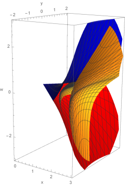
Figure 22: Spheres inside the attainable set for the second problem

5 Conclusion

The first problem is fundamentally different from the second one by the following properties of the optimal synthesis:

• some optimal trajectories change causal type,

• extremal trajectories have cut points on the Martinet surface $\Pi$,

• the optimal synthesis is two-valued on $\Pi$,

• the sub-Lorentzian distance is nonsmooth on $\Pi$ and suffers a discontinuity of the first kind at some points of the boundary of the attainable set $\partial\mathcal{A}_{1}$,

• the sub-Lorentzian sphere $S$ is a manifold with boundary.

These features are associated with non-trivial intersection of the attainable set $\mathcal{A}_{1}$ (the causal future of the initial point $q_{0}$) and the Martinet surface $\Pi$ for the first problem.

The optimal synthesis in the second problem is qualitatively the same as in the sub-Lorentzian problem on the Heisenberg group [13].

List of Figures

1. 1 The set $U_{1}$
2. 3.2 Invariant set
3. 3.2 Invariant set
4. 3.3.2 Normal extremals
5. 3.3.2 Normal extremals
6. 10 Stratification in the image of $\operatorname{Exp}\nolimits$
7. 11 Plot of $\eta\mapsto d(0,1,\eta+1/24)$
8. 3.8 Sub-Lorentzian sphere
9. 3.8 Sub-Lorentzian sphere
10. 3.8 Sub-Lorentzian sphere
11. 3.8 Sub-Lorentzian sphere
12. 4.2 Invariant set
13. 22 Spheres inside the attainable set for the second problem

References

- [1] R. Montgomery, A tour of subriemannnian geometries, their geodesics and applications, Amer. Math. Soc., 2002
- [2] A. Agrachev, D. Barilari, U. Boscain, A Comprehensive Introduction to sub-Riemannian Geometry from Hamiltonian viewpoint, Cambridge Studies in Advanced Mathematics, Cambridge Univ. Press, 2019
- [3] M. Grochowski, Geodesics in the sub-Lorentzian geometry. Bull. Polish. Acad. Sci. Math., 50 (2002).
- [4] M. Grochowski, Normal forms of germs of contact sub-Lorentzian structures on . Differentiability of the sub-Lorentzian distance. J. Dynam. Control Systems 9 (2003), No. 4.
- [5] M. Grochowski, Properties of reachable sets in the sub-Lorentzian geometry, J. Geom. Phys. 59(7) (2009) 885–900.
- [6] M. Grochowski, Reachable sets for contact sub-Lorentzian metrics on . Application to control affine systems with the scalar input, J. Math. Sci. (N.Y.) 177(3) (2011) 383–394.
- [7] M. Grochowski, On the Heisenberg sub-Lorentzian metric on , GEOMETRIC SINGULARITY THEORY, BANACH CENTER PUBLICATIONS, INSTITUTE OF MATHEMATICS, POLISH ACADEMY OF SCIENCES, WARSZAWA, vol. 65, 2004.
- [8] M. Grochowski, Reachable sets for the Heisenberg sub-Lorentzian structure on . An estimate for the distance function. Journal of Dynamical and Control Systems, vol. 12, 2006, 2, 145–160.
- [9] D.-C. Chang, I. Markina and A. Vasil’ev, Sub-Lorentzian geometry on anti-de Sitter space, J. Math. Pures Appl., 90 (2008), 82–110.
- [10] A. Korolko and I. Markina, Nonholonomic Lorentzian geometry on some H-type groups, J. Geom. Anal., 19 (2009), 864–889.
- [11] E. Grong, A. Vasil’ev, Sub-Riemannian and sub-Lorentzian geometry on and on its universal cover, J. Geom. Mech. 3(2) (2011) 225–260.
- [12] M. Grochowski, A. Medvedev, B. Warhurst, 3-dimensional left-invariant sub-Lorentzian contact structures, Differential Geometry and its Applications, 49 (2016) 142–166
- [13] Yu. L. Sachkov, E.F. Sachkova, Sub-Lorentzian distance and spheres on the Heisenberg group, Journal of Dynamical and Control Systems volume 29, pages 1129–1159 (2023)
- [14] A. Agrachev, Yu. Sachkov, Control theory from the geometric viewpoint, Berlin Heidelberg New York Tokyo. Springer-Verlag, 2004.
- [15] L.S. Pontryagin, V. G. Boltyanskii, R. V. Gamkrelidze, E.F. Mishchenko, Mathematical Theory of Optimal Processes, New York/London. John Wiley & Sons, 1962.
- [16] Yu. Sachkov, Introduction to geometric control, Springer, 2022.
- [17] A.Agrachev, B. Bonnard, M. Chyba, I. Kupka, Sub-Riemannian sphere in Martinet flat case. J. ESAIM: Control, Optimisation and Calculus of Variations, 1997, v.2, 377–448
- [18] Yu. L. Sachkov, Left-invariant optimal control problems on Lie groups that are integrable by elliptic functions, Russian Math. Surveys, 78:1 (2023), 65–163
- [19] A.Ardentov, Yu. L. Sachkov, Tiren Huang, Xiaoping Yang, Extremals in the Engel group with a sub-Lorentzian metric, Sbornik: Mathematics, 209:11 (2018), 3–31
- [20] E.T. Whittaker, G.N. Watson, A Course of Modern Analysis. An introduction to the general theory of infinite processes and of analytic functions; with an account of principal transcendental functions, Cambridge University Press, Cambridge 1996.
- [21] D. F. Lawden, Elliptic Functions and Applications, Springer, 1989
- [22] Krantz S. G., Parks H. R., The Implicit Function Theorem: History, Theory, and Applications, Birkauser, 2001.
- [23] Yu. L. Sachkov, Existence of sub-Lorentzian length maximizers, Differential equations, 59, 12, 1702–1709 (2023)
- [24] Agrachev A.A., Geometry of optimal control problems and Hamiltonian systems. In: Nonlinear and Optimal Control Theory, Lecture Notes in Mathematics. CIME, 1932, Springer Verlag, 2008, 1–59.
- [25] Yu. L. Sachkov, The Maxwell set in the generalized Dido problem, Sbornik: Mathematics, 197 (2006), 4: 595–621.