SSP-GNN: Learning to Track
via Bilevel Optimization
††thanks: ∗Corresponding author
Abstract
We propose a graph-based tracking formulation for multi-object tracking (MOT) where target detections contain kinematic information and re-identification features (attributes). Our method applies a successive shortest paths (SSP) algorithm to a tracking graph defined over a batch of frames. The edge costs in this tracking graph are computed via a message-passing network, a graph neural network (GNN) variant. The parameters of the GNN, and hence, the tracker, are learned end-to-end on a training set of example ground-truth tracks and detections. Specifically, learning takes the form of bilevel optimization guided by our novel loss function. We evaluate our algorithm on simulated scenarios to understand its sensitivity to scenario aspects and model hyperparameters. Across varied scenario complexities, our method compares favorably to a strong baseline.
Index Terms:
feature-aided tracking, data association, GNNI Introduction
Multi-target and multi-object tracking (MOT) is often a necessary step in larger systems that address real-world challenges. Examples include tracking pedestrians in the context of autonomous driving, tracking animals and birds to understand environmental factors, and tracking players in team sports to analyze plays.
MOT remains a challenging problem even in scenarios where detections contain features (attributes) that could potentially help associate across target identities and distinguish targets from clutter. One of the challenges in feature-aided tracking is to exploit feature vectors of arbitrary (possibly high) dimensions. Another challenge is to reason jointly and optimally about attributes and target dynamics.
Learning-based approaches to tracking [31, 26] learn key components of a tracker (e.g., data association) directly from annotated training data. Recently, approaches to neural message passing [11] have been adopted by [5] to formulate tracking on a detection graph (where a detection graph is instantiated for a temporal window given all the measurements/detections). However, predicting which pairs of detections should be linked without inferring complete tracks, while computationally efficient, may be suboptimal.
We propose an end-to-end bilevel formulation for learning MOT, where the inner optimization (tracking) is accomplished via a successive shortest paths (SSP) algorithm on a tracking graph [6, 32] with edge costs. Given these costs, SSP finds a solution that is guaranteed to be optimal. In our outer optimization problem we learn parameters of a function that computes the cost of each edge in the tracking graph given detections that include attributes. The edge-cost prediction function takes the form of a graph neural network (GNN).
Learning GNN parameters requires solving a bilevel optimization problem that is different from those proposed earlier, e.g. [26, 16]. Specifically, we derive a novel loss function defined with respect to SSP-computed tracks and the ground-truth tracks and an algorithm to learn the GNN parameters by gradient descent. At each iteration, GNN parameters are updated to increase the cost of incorrect tracks, effectively learning from (tracking) mistakes.
The contributions of our paper are as follows:
- •
-
•
A novel use of SSP for inner optimization, guaranteeing an optimal solution satisfying tracking constraints.
-
•
Quantitative analysis of our algorithm on a diverse set of synthetic scenarios and comparison with a strong baseline that relies on GNN but does not employ global path optimization.
II Related Work
Learning approaches to tracking In many domains, using machine-learning tools to find optimal parameters for a tracking algorithm from data have been shown to outperform hand-crafting and hand-tuning an algorithm. In the computer vision domain, learning-based approaches to multi-object tracking have taken many different forms. [31] Demonstrated a Markov decision process (MDP) capable of initiating and terminating target tracks; parameters of this MDP were learned from data. In [20] recurrent neural networks were used in an end-to-end framework. Specifically, in [20] a target’s state was maintained by a dedicated recurrent neural network (RNN); assignment of measurements to target tracks and track creation was estimated via a long-short-term memory (LSTM) neural network. A transformer neural network was used in [19] as a unified formulation for detecting (new) targets, extending tracks, and creating new tracks.
Graph-based tracking via classical methods Application of graph-based and linear-programming (LP) methods to multi-target tracking has a long history, e.g., [6], and includes recent attempts to combine graph-based tracking with multi-hypothesis tracking (MHT) [9]. Graph-based tracking has shown to be effective in computer vision where it is often employed with a tracking-by-detection paradigm where tracking is reduced to the grouping of detections (bounding boxes) proposed by a (target class specific) object detector.
An early graph-based method of [32] proposed the general form of a tracking graph and solved for an unknown number of targets via repeated invocation of min-cost flow. The computational complexity was reduced in [24] by introducing augmenting paths, thus extending an existing tracking solution to include an additional target instead of starting from scratch. While [32] and [24] performed tracking in the image plane, tracking on the ground plane from multiple camera views via K-shortest-paths (KSP) algorithm was proposed in [3]. Approaches mentioned thus far assumed that targets dynamics are Markovian and targets move independently of each other. An approach to extend LP-based tracking to take into account long-term (group) behavior was proposed in [18]. During training, their method alternated between learning behavior patterns and fitting trajectories to data given the observations and priors given by the learned patterns.
Graph-based tracking via neural methods A significant limitation of early graph-based approaches [32, 24, 3] is the requirement to hand-craft scalar costs on tracking graph edges. However, in many real-world scenarios where we wish to apply feature-aided tracking, measurements (detections) in addition to containing positional information also include (high-dimensional) vectors of attributes, such as re-identification (ReID) features. Neural networks could learn a mapping from these high-dimensional attributes to scalar edge weights, but deriving an end-to-end learnable method is nontrivial. Among the first attempts to apply neural methods to graph-based tracking, the approach of [26] stands out for formulating learning and tracking as bilevel [33] optimization. Specifically, in [26] the high-level optimization problem solved for the neural network parameters, while the lower-level problem was a constrained LP that solved a tracking-by-detection problem over a temporal window of pre-defined length. The bilevel approach of [26] was revisited in [16], but instead of relying on the implicit function theorem to deal with the inner LP problem, the latter used KKT conditions to compute the gradient at the lower problem’s optimum.
Recent advances in neural methods for graph-structured problems, such as graph neural networks (GNNs) [10] led to advances in graph-based tracking. Inspired by the neural message-passing on graphs method of [11], the authors of [5] proposed to learn a function to estimate edge probabilities in a tracking graph. This approach was extended in [7] to jointly solve for short-term and long-term tracking. While the approaches of [5, 7] require a batch of frames, and thus operate with a constant lag, approaches of [30, 19] require only the current frame to manage tracks. The ideas of [11] were adopted in [17] to develop a neural-enhanced message-passing data association algorithm.
Neural approaches to optimization Learning-based approaches to MOT mentioned thus far solve the underlying assignment problem using classical methods e.g., LP. An approach to solve quadratic optimization as a layer in a neural network was proposed in [2]. In [23], the matrix of association costs was updated using Sinkhorn-Knopp’s algorithm [27] to satisfy MOT constraints. A differentiable graph matching layer was proposed in [12] and used to associate graphs formed on detections across time frames.
Our contribution We draw on [10, 11] and [5] to formulate a GNN that infers edge costs on a graph structure, but unlike [5] our inner optimization with SSP ensures that track predictions are globally optimal and satisfy constraints. We demonstrate in Section IV that our method compares favorably to a GNN-based method without such inner optimization. Our method is similar to that of [16] in forming a bilevel problem during training, but we show in Section III-D that our inner optimization with SSP has lower computational complexity.
III Approach
Let denote target state and let denote measurement (detection). A detection at time may originate from one of the targets (if present) or from clutter (i.e., it’s a false alarm).
We adopt a sliding-window approach, where tracking is performed on a batch of data frames over a temporal window of length . In a complete system, separate logic is used to produce an output that takes into account the tracking solution from the previous temporal window. Figure 1 shows the system diagram of our approach.
III-A Graph-based formulation
Within the batch of data frames, we solve the tracking problem by casting it in a graph-based formulation [32, 24]. Given a temporal window our objective is to group into a set of paths in a tracking graph with positive and negative edge costs. The set may be empty if the tracker doesn’t predict any tracks.
III-B The detection graph and the tracking graph
Given detections in a temporal window with frames, we construct a detection graph . Nodes in are in one-to-one correspondence with detections in . An edge exists between and if and the location components of and satisfy gating constraints. The use of is standard [26, 16] to handle short-duration obscuration (occlusion) of a target. In Fig. 2(a) we show an example of for and . Two paths that satisfy node-disjoint constraints are shown.
Given , we define its companion tracking graph , whose topology follows [6, 32]. In particular, every node in is represented by a pair of “twin” nodes in . Furthermore, contains source and terminal nodes with edges from and to defined in a way as to allow every detection to either correspond to a tracks’s birth or its termination. Fig. 2(b) shows the tracking graph derived from its ; the paths (tracks) in originate in , pass through “twin” nodes and terminate in .

Computing edge-costs of a tracking graph via MPN Let be a function, parameterized by for computing edge costs in a graph
| (1) |
Our takes the form of a message-passing network (MPN) [11], a specialization of a graph neural net (GNN) [10]. We adopt the ideas of [11] and [14] as implemented in [5].
Let be an integer representing the number of message passing layers (iterations), be the edge set, and be the vertex set of . Let be the embedding of edge at iteration and similarly be the embedding of the vertex at iteration . We assume without loss of generality that node is ahead of node in time.
Messages are computed using the functions and which take the form of learnable multi-layer perceptions. In our implementation, as suggested by [5], consists of two independently parameterized functions which are specialized for forward and backward in time messages respectively. The readout function , also a learnable MLP, then computes the edge cost by aggregating the final attributes of the forward and backward in time edges between each pair of nodes. The parameters of these four functions comprise the vector .
III-C End-to-end learning for tracking
Optimization criterion To derive our algorithm to learn we need a differentiable optimization criterion (a loss function). The loss function should be defined with respect to the ground-truth tracks (paths) and the predicted ones .
Given with edge costs we rewrite the edge costs as a real-valued function . For a track (path) , we define (with slight abuse of notation) , where are entrance and exit costs. For a set of paths , we define .
We define the set loss for two sets of paths as
| (2) |
The first term is defined and the second .
The following claim follows immediately from the properties of an SSP algorithm.
Claim 1.
Let be the estimated set of paths. Then and for all , .
The next claim confirms that optimizing converges to .
Claim 2.
Suppose that the cost of each unique set of mutually disjoint paths in the tracking graph is unique. Then if and only if as sets. If these equivalent conditions hold, as well.
The first part follows from the fact that is the global optimum, but so is , by definition. The second part follows by showing that , and hence is zero.
Bilevel optimization to learn MPN parameters We formulate the following bilevel optimization problem [8, 33, 21] to find the optimal set of GNN parameters given ground-truth paths :
| (3) |
The problem defined in Equation 3 is non-trivial: the outer objective is non-linear, while the inner objective is stated in terms of a constrained search for minimum-cost paths in a graph. Applying the chain rule to our loss, yields
| (4) |
where .
In practice, we implement optimization of in Equation 3 via a two-stage learning algorithm. In Stage I, inspired by [22] which introduced MCMC data association moves, we “perturb” to pre-compute a fixed-size set of negative examples . Generating does not require running the SSP algorithm.
Let be one of the paths (tracks) obtained via perturbation, and let be a ground-truth path. In general, given , it is not the case that every has a higher cost than every . Nevertheless for Stage I we define
| (5) |
for some margin . And we can extend this to the entire set of all the paths obtained by perturbing . Optimizing leads to which serves as a “warm start” for Stage II which implements Equation 3.
Our end-to-end learning approach is defined in Algorithm 2; extending it to multiple training graphs is straightforward. We will demonstrate in the experiments section that learning this way yields a stable training algorithm.
III-D Computational Complexity
In our analysis, to provide a fair comparison between our proposed algorithm and related methods we focus only on forward inference of the inner optimization problem used to compute from . In our implementation, this is solved using SSP, specifically the -shortest-paths algorithm. As shown in [3], this algorithm has a worst-case time complexity of , where is the number of paths/tracks found by the algorithm and and refer to the number of nodes and edges, respectively, contained in the graph . The size and topology of depends on , and therefore is a function of both the size of the temporal window and the number of targets and false alarms.
In contrast, linear programming (LP)-based approaches to the min-cost flow problem have an average-case polynomial time complexity in the size of [1]. This also applies to more recent approaches presented in [26] and [16], which embed the LP solution as a differentiable layer within a multi-layer perceptron.111Note that [16] transforms the LP problem to a regularized quadratic program; however, the transformed problem has the same time complexity. The proposed SSP-GNN algorithm blends the edge-cost expressivity of learning-based methods with the reduced time complexity of SSP methods.
IV Experiments
We conduct extensive experiments to demonstrate the advantages of our method and to assess the impact of a variety of model and scenario attributes on performance.
IV-A Train and Test Scenarios
Our synthetic data is generated using Stone Soup 222https://github.com/dstl/Stone-Soup/, an open-source framework. We generate diverse scenarios with multiple targets using constant velocity and Ornstein-Uhlenbeck motion models. When generating detections, we fix the detection probability at 1.0 except in Table LABEL:tab:p_d_exps which investigates the effects of an imperfect detector, and we fix measurement error standard deviation at . We refer to target features as re-identification (ReID) as is common in computer vision. However, our approach can generalize to other features and sensing modalities, e.g., [15]. Our ReID features are drawn from a mixture of Gaussians (MoG) distributions. We control the “strength” of ReID features by changing the amount of overlap between the foreground and background distributions and define categories in terms of KL divergence: very weak (0.02 nats/0.029 bits), weak (0.5 nats/0.721 bits), moderate (3.125 nats/4.508 bits), and strong (12.5 nats/18.034 bits).
IV-B Implementation Details
Given a pair of detections with we follow [16] to encode their spatio-temporal constraint into our latent representation. We denote the kinematic (spatial) component of a detection as , , the ReID component as , . For a node in , we define . For an edge between the two detections in , we define . We use 2D scenarios and 2D ReID features, i.e., and .
Tracking graph and inference We instantiate and learn parameters on the detection graph as shown in Fig. 2(a). Then, assigns scalar costs to the edges in . We copy these edge costs from to by associating each edge with the edge between the pair of twin nodes associated with and the pair of twin nodes associated with in . We assign a cost of 0 to the edges within the twin nodes, shown as red arrows in Figure 2(b). This formulation allows us to use the GNN-computed as edge costs for the SSP algorithm to optimize over . Detection and tracking graphs are represented via NetworkX 333https://networkx.org/ except for GNN learning and inference the detection graph is converted to a Deep Graph Library (DGL) [29] object.
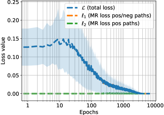
Training We use the Adam optimizer [13] with a learning rate of 0.001. Fig. 3 demonstrates a typical loss curve across 20 re-initialized training trials on the same train set. In practice we observe that tends to dominate total loss because (a) our Stage I bootstrapping guarantees that at epoch 0 and (b) captures the more trivial problem of simply keeping the ground truth paths sufficiently negative in cost, while addresses the more difficult problem of predicting the ground truth paths over competing sets of paths.
IV-C Evaluation Metrics
Our method is inspired by [5, 16], etc., which were developed for tracking objects in video sequences. These methods tend to be evaluated with respect to Multiple Object Tracking Accuracy (MOTA) [4]. While our method is applicable to tracking extended targets in video sequences, we generate point observations in our Stone Soup simulation. We therefore report the MOTA metrics calculated with respect to the point observations for all of our experiments. We also report GOSPA [25] and SIAP[28] metrics when comparing our model’s performance to a filter-based tracker provided by Stone Soup.
Following [4], MOTA is defined as:
| (6) |
where is the time step, is the number of false positives, is the number of false negatives, and is the number of identity switches. We report MOTA, as well as each constituent metric as ratios with the number of ground truth detection’s (rates). Since we control data generation, we can utilize ID-based matching between tracks and true detections instead of the traditional Hungarian matching algorithm typically used for computer vision applications. The ability to perform more straightforward ID-based matching for evaluation is one advantage of using synthetic data.
Both GOSPA and SIAP metrics are popular evaluation methods for comparing predicted tracks to continuous ground-truth object paths. GOSPA quantifies localization and cardinality errors, and SIAP completeness (C), ambiguity (A), spuriousness (S), and positional error, provide a more complete insight into the accuracy of associations between predicted tracks and ground truth objects. We report metrics summed over all time frames for GOSPA and averaged for SIAP.
IV-D Qualitative Demonstration
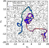
For demonstration, in Figure 4 we show a sample SSP-GNN result trained on one scenario. Both the training and test scenarios last 100 timesteps and include three targets with randomly-generated lifespans following Ornstein-Uhlenbeck dynamics. Each scenario uses moderate strength ReID features and 20 uniformly distributed false alarms per frame. We observe that our algorithm generalizes well to the test scenario (the circled predicted tracks follow ground truth paths). The MOTA score is 0.993 for train scenario and 0.987 for the test scenario.
IV-E Quantitative Evaluations
Since we are working with synthetic data, we can generate datasets of varying sizes and complexity. This enables isolating specific aspects of train and test scenarios to examine the effect on our model. However, since not all published methods report such analysis, and there is no standardized evaluation protocol, our results cannot be immediately compared to others reported in literature.
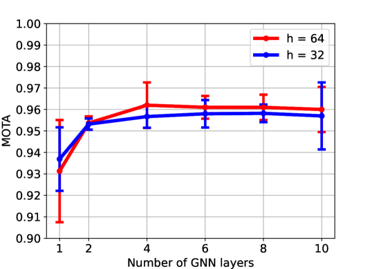
Effect of GNN hyperparameters We first determine the optimal value of two hyperparameters used in configuring the graph neural network: number of message passing layers and size of the hidden layers in all used MLP’s. Figure 5 shows the MOTA performance of the model on fixed train and test sets with variable number of GNN layers and hidden dimension size. The scenarios involve multiple ground truth tracks with constant velocity motion models, moderate strength ReID features, and 8 false alarms per frame in expectation.
As the number of message passing layers in the graph neural network increases model performance also tends to increase until saturation is reached, at which point it largely levels out. Using a hidden dimension size of 64 produced the best results overall, and it achieves saturation at 4 GNN layers. Therefore, we use these hyperparameter values in all experiments going forward. When working with substantially different environments from our synthetic data, the optimal values for these hyperparameters would need to be adapted.
Comparison to baselines We compare our SSP-GNN tracker to an Extended Kalman Filter (EKF) based multi-object tracker and Edge-Belief GNN (based on [5]) . The EKF tracker implementation is provided by the Stone Soup library. Although EKF only processes the kinematic component of measurements and is an online method (while ours is offline/batch-based), it establishes a reference point in our comparison.
The Edge-Belief GNN algorithm [5] uses the same MPN architecture as our SSP-GNN, but instead of predicting edge costs, Edge-Belief GNN individually estimates the probability of an edge in the detection graph being part of a track or not. This is accomplished by modifying to output sigmoid rather than logits. During inference, edge beliefs are rounded up or down to yield binary predictions, and a follow-on edge traversal heuristic ensures that the computed paths are node-disjoint. We observed that the Edge-Belief GNN tends to produce short (spurious) tracks; we added a post processing step which removes tracks shorter than a set length in order to strengthen the baseline (empirically we found minimum path threshold was optimal).
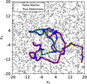
Figure 6 shows tracks produced by an SSP-GNN model and Edge-Belief GNN model on a test scenario. In this scenario, there are several instances where two tracks intersect. Our model correctly maintains target tracks on the left, while it swaps paths causing two identity switches on the right. Edge-belief GNN tends to fragment or deviate from tracks to nearby false alarms much more frequently than the SSP-GNN.
Table LABEL:tab:baseline-comparisons compares Edge-Belief GNN, SSP-GNN, and EKF on similar scenarios. As inferred from the visual demonstration, the false negative rate is nearly twice that of SSP-GNN. Edge-Belief also has a substantially higher identity switch rate, indicating track fragmenting, but it does achieve a comparable false positive rate to our model.
Table LABEL:tab:edgebelief_vs_ssp compares Edge-Belief GNN and SSP-GNN on similarly structured scenarios, but with increased difficulty due to false alarm rate and ReID feature weakness, (the EKF tracker is omitted as ignoring ReID features makes it uncompetitive). SSP-GNN consistently outperforms Edge-Belief by a sizable margin, which is even more pronounced in harder regimes.
Because the Edge-Belief GNN baseline uses the same underlying message passing algorithm as SSP-GNN, we ascribe the observed performance increase to bilevel optimization. The SSP solver allows our model to properly weigh various trade-offs in the context of the full scenario. For instance it can weigh the cost of including a series of positive cost edges that would link otherwise disparate tracks versus the extra entrance/exit cost of inferring more tracks.
| Tracker | Metrics | |||||||||||
|---|---|---|---|---|---|---|---|---|---|---|---|---|
| MOTA | SIAP | GOSPA | ||||||||||
| MOTA | FPR | FNR | IDS Rate | C (1) | A (1) | S (0) | Pos. Err. (0) | Dist. | Local. | Missed | False | |
| EKF | ||||||||||||
| Edge-Belief | 0.9150.008 | |||||||||||
| SSP-GNN (ours) | 0.9420.050 | |||||||||||
| Tracker | FA Rate | ReID Strength | MOTA |
|---|---|---|---|
| Edge-Belief | Moderate | 0.862 0.012 | |
| SSP-GNN | Moderate | 0.950 0.019 | |
| Edge-Belief | Weak | 0.826 0.008 | |
| SSP-GNN | Weak | 0.952 0.006 | |
| Edge-Belief | Moderate | 0.656 0.032 | |
| SSP-GNN | Moderate | 0.891 0.034 | |
| Edge-Belief | Weak | 0.633 0.018 | |
| SSP-GNN | Weak | 0.873 0.023 |
Effect of ReID feature strength and noisy dimensions We use one trajectory following an Ornstein–Uhlenbeck motion model over a 50 timestep period with a high false alarm rate (expected 30 per frame). Table LABEL:tab:reID-strength shows a clear positive correlation between model performance and ReID feature strength. The two extremes of the table also indicate that the model leverages strong ReID features effectively, while also allowing for good motion-based predictions when ReID features are highly unreliable.
While it is clear that our method can handle higher-dimensional ReID features, it is interesting to consider a case where the dimensions are not equally informative. We therefore constructed scenarios with up to ten additional ReID feature dimensions filled with i.i.d. noise. While training took longer, our learned tracker did not suffer any noticeable degradation in accuracy, indicating that the algorithm is able to find informative components of ReID and ignore the rest.
| ReID Str. | MOTA | FP Rate | FN Rate | IDS Rate |
|---|---|---|---|---|
| Strong | 0.961 0.031 | |||
| Moderate | 0.918 0.023 | |||
| Weak | 0.909 0.009 | |||
| Very weak | 0.893 0.021 |
Table LABEL:tab:reID-noisy-dimensions demonstrates that the model is resilient to added dimensions of noise in the ReID features. There is a very slight drop in prediction quality as initial noisy dimensions are added, but then a sudden increase at 10. We attribute this to a random effect, although there could be an unforeseen interaction where adding extra noise incentives the model to learn the meaningful relations more robustly on our limited training set.
| Noisy Dims | MOTA | FP Rate | FN Rate | IDS Rate |
|---|---|---|---|---|
| 0 | 0.935 0.021 | |||
| 2 | 0.929 0.010 | |||
| 5 | 0.927 0.011 | |||
| 10 | 0.959 0.015 |
| FA per frame | MOTA | FP Rate | FN Rate | IDS Rate |
|---|---|---|---|---|
| 2 | 0.994 0.004 | |||
| 5 | 0.979 0.007 | |||
| 10 | 0.938 0.047 | |||
| 20 | 0.900 0.040 | |||
| 30 | 0.907 0.017 |
Effect of false alarm rate Table LABEL:tab:fa_freq displays the performance of our method at a variety of expected numbers of false alarms per frame. The performance is nearly optimal when false alarms are sparse, and deteriorates gracefully as false alarms are added, however it seems to level off and not drop below a MOTA score of about 0.9. This indicates that our algorithm is capable of capitalizing on easier regimes with relatively few false positives, while also adapting to hard environments where false alarms significantly outnumber ground truth tracks.
Effect of the training set size Table LABEL:tab:training-set-size test our model with a variety of training set sizes. Our experiments use limited size training sets so as to run multiple trials. Real world applications would likely train on more data than we use, so it is important that model accuracy scales with training set size.
This experiment uses a diverse array of scenarios using constant velocity and Ornstein–Uhlenbeck motion models with variable ReID strength (moderate to weak) and up to 5 ground truth tracks. Table LABEL:tab:training-set-size shows a positive correlation between number of graphs in the training set and model performance. Learned tracker consistency, represented by standard deviation, also improves substantially with training set size.
| Train Set | ||||
|---|---|---|---|---|
| Size | MOTA | FP Rate | FN Rate | IDS Rate |
| 1 | 0.894 0.046 | |||
| 5 | 0.937 0.032 | |||
| 10 | 0.954 0.006 | |||
| 20 | 0.958 0.019 | |||
| 30 | 0.963 0.007 |
Effect of lower detection probability Finally, we consider the effect of an imperfect detector i.e., . To allow the model to select trajectories that skip time steps, we modify the tracking graph to contain edges between non-adjacent timesteps up to three apart.
In Table LABEL:tab:p_d_exps we observe a drop in MOTA of around 0.04 when detection probability decreases from 1.0 to 0.95, as adding missed detections increases the complexity of the representation that must be learned. Our model performance is resilient between detection probabilities of 0.95 to 0.85. From 0.85 to 0.8, there is another drop in performance, which may be due to the increasing prevalence of enduring missed detections lasting beyond what the model is capable of considering.
| MOTA | FP Rate | FN Rate | IDS Rate | |
|---|---|---|---|---|
| 1.0 | 0.978 0.001 | |||
| 0.95 | 0.957 0.013 | |||
| 0.9 | 0.945 0.020 | |||
| 0.85 | 0.944 0.012 | |||
| 0.8 | 0.913 0.017 |
V Conclusions
We presented a novel trainable approach for graph-based multi-object tracking. Our approach predicts edge costs using a message passing GNN, then relies on a globally optimal and computationally-efficient path-finding algorithm to form tracks that satisfy the required constraints. The message-passing network can be learned end-to-end in a bilevel optimization framework that is different from prior work. We thoroughly investigated model performance on a variety of scenarios. Our learned tracker compares favorably to a strong baseline. In our future work, we plan to focus on computationally-efficient extensions to our graph formulation and the message-passing network to optimally handle long-term occlusions.
VI Acknowledgements
We thank the anonymous reviewers for their feedback and Samuel C. Buckner for helpful discussions. Earlier work funded by U.S. Office of Naval Research Code 321.
References
- [1] R. K. Ahuja, T. L. Magnanti, and J. B. Orlin. Network Flows: Theory, Algorithms, and Applications. Prentice-Hall, 1993.
- [2] B. Amos and J. Z. Kolter. OptNet: Differentiable optimization as a layer in neural networks. In D. Precup and Y. W. Teh, editors, Proceedings of the 34th International Conference on Machine Learning, volume 70 of Proceedings of Machine Learning Research, pages 136–145. PMLR, 06–11 Aug 2017.
- [3] J. Berclaz, F. Fleuret, E. Turetken, and P. Fua. Multiple object tracking using K-shortest paths optimization. IEEE Transactions on Pattern Analysis and Machine Intelligence, 33(9):1806–1819, 2011.
- [4] K. Bernardin and R. Stiefelhagen. Evaluating multiple object tracking performance: The clear mot metrics. EURASIP Journal on Image and Video Processing, 2008, 01 2008.
- [5] G. Brasó and L. Leal-Taixé. Learning a neural solver for multiple object tracking. In IEEE/CVF Conference on Computer Vision and Pattern Recognition (CVPR), June 2020.
- [6] D. Castañon. Efficient algorithms for finding the K best paths through a trellis. IEEE Transactions on Aerospace and Electronic Systems, 26(2):405–410, 1990.
- [7] O. Cetintas, G. Brasó, and L. Leal-Taixé. Unifying short and long-term tracking with graph hierarchies. In Proceedings of the IEEE/CVF Conference on Computer Vision and Pattern Recognition (CVPR), pages 22877–22887, June 2023.
- [8] B. Colson, P. Marcotte, and G. Savard. An overview of bilevel optimization. Annals of Operations Research, 153:235–256, Sept. 2007.
- [9] S. P. Coraluppi, C. A. Carthel, and A. S. Willsky. Multiple-hypothesis tracking and graph-based tracking extensions. Journal of Advances in Information Fusion, 14(2), 2019.
- [10] M. Defferrard, X. Bresson, and P. Vandergheynst. Convolutional neural networks on graphs with fast localized spectral filtering. In Proceedings of the 30th International Conference on Neural Information Processing Systems, NeurIPS’16, page 3844–3852, Red Hook, NY, USA, 2016. Curran Associates Inc.
- [11] J. Gilmer, S. S. Schoenholz, P. F. Riley, O. Vinyals, and G. E. Dahl. Neural message passing for quantum chemistry. In D. Precup and Y. W. Teh, editors, Proceedings of the 34th International Conference on Machine Learning, volume 70 of Proceedings of Machine Learning Research, pages 1263–1272, International Convention Centre, Sydney, Australia, 06–11 Aug 2017. PMLR.
- [12] J. He, Z. Huang, N. Wang, and Z. Zhang. Learnable graph matching: Incorporating graph partitioning with deep feature learning for multiple object tracking. In Proceedings of the IEEE/CVF Conference on Computer Vision and Pattern Recognition (CVPR), pages 5299–5309, June 2021.
- [13] D. P. Kingma and J. Ba. Adam: A method for stochastic optimization, 2017.
- [14] T. Kipf, E. Fetaya, K.-C. Wang, M. Welling, and R. Zemel. Neural relational inference for interacting systems. In J. Dy and A. Krause, editors, Proceedings of the 35th International Conference on Machine Learning, volume 80 of Proceedings of Machine Learning Research, pages 2688–2697. PMLR, 10–15 Jul 2018.
- [15] J. LeNoach, M. Lexa, and S. Coraluppi. Feature-aided tracking techniques for active sonar applications. In IEEE 24th International Conference on Information Fusion (FUSION), pages 1–7. IEEE, 2021.
- [16] S. Li, Y. Kong, and H. Rezatofighi. Learning of global objective for network flow in multi-object tracking. In 2022 IEEE/CVF Conference on Computer Vision and Pattern Recognition (CVPR), pages 8845–8855. IEEE, 2022.
- [17] M. Liang and F. Meyer. Neural enhanced belief propagation for data association in multiobject tracking. In 2022 25th International Conference on Information Fusion (FUSION), pages 1–7, 2022.
- [18] A. Maksai, X. Wang, F. Fleuret, and P. Fua. Non-Markovian globally consistent multi-object tracking. In Proceedings of the IEEE International Conference on Computer Vision (ICCV), Oct 2017.
- [19] T. Meinhardt, A. Kirillov, L. Leal-Taixé, and C. Feichtenhofer. Trackformer: Multi-object tracking with transformers. In Proceedings of the IEEE/CVF Conference on Computer Vision and Pattern Recognition (CVPR), pages 8844–8854, June 2022.
- [20] A. Milan, S. H. Rezatofighi, A. Dick, I. Reid, and K. Schindler. Online multi-target tracking using recurrent neural networks. In Proceedings of the AAAI conference on Artificial Intelligence, volume 31, 2017.
- [21] P. Ochs, R. Ranftl, T. Brox, and T. Pock. Bilevel optimization with nonsmooth lower level problems. In J.-F. Aujol, M. Nikolova, and N. Papadakis, editors, Scale Space and Variational Methods in Computer Vision, pages 654–665, Cham, 2015. Springer International Publishing.
- [22] S. Oh, S. Russell, and S. Sastry. Markov chain monte carlo data association for multi-target tracking. IEEE Transactions on Automatic Control, 54(3):481–497, 2009.
- [23] I. Papakis, A. Sarkar, and A. Karpatne. GCNNMatch: Graph convolutional neural networks for multi-object tracking via sinkhorn normalization. arXiv preprint arXiv:2010.00067, 2020.
- [24] H. Pirsiavash, D. Ramanan, and C. C. Fowlkes. Globally-optimal greedy algorithms for tracking a variable number of objects. In CVPR 2011, pages 1201–1208, 2011.
- [25] A. S. Rahmathullah, A. F. Garcia-Fernandez, and L. Svensson. Generalized optimal sub-pattern assignment metric. In 2017 20th International Conference on Information Fusion (Fusion). IEEE, July 2017.
- [26] S. Schulter, P. Vernaza, W. Choi, and M. Chandraker. Deep network flow for multi-object tracking. In 2017 IEEE Conference on Computer Vision and Pattern Recognition (CVPR), pages 2730–2739, 2017.
- [27] R. Sinkhorn and P. Knopp. Concerning nonnegative matrices and doubly stochastic matrices. Pacific Journal of Mathematics, 21(2):343–348, 1967.
- [28] P. Votruba, R. Nisley, R. Rothrock, and B. Zombro. Single integrated air picture (SIAP) metrics implementation. In Tech. Rep. Single Integrated Air Picture (SIAP) System Engineering Task Force, Arlington, VA, 2001.
- [29] M. Wang, D. Zheng, Z. Ye, Q. Gan, M. Li, X. Song, J. Zhou, C. Ma, L. Yu, Y. Gai, T. Xiao, T. He, G. Karypis, J. Li, and Z. Zhang. Deep graph library: A graph-centric, highly-performant package for graph neural networks. arXiv preprint arXiv:1909.01315, 2019.
- [30] Y. Wang, K. Kitani, and X. Weng. Joint Object Detection and Multi-Object Tracking with Graph Neural Networks. arXiv:2006.13164, 2020.
- [31] Y. Xiang, A. Alahi, and S. Savarese. Learning to track: Online multi-object tracking by decision making. In Proceedings of the IEEE International Conference on Computer Vision (ICCV), December 2015.
- [32] L. Zhang, Y. Li, and R. Nevatia. Global data association for multi-object tracking using network flows. In 2008 IEEE Conference on Computer Vision and Pattern Recognition, pages 1–8, 2008.
- [33] Y. Zhang, P. Khanduri, I. Tsaknakis, Y. Yao, M. Hong, and S. Liu. An introduction to bi-level optimization: Foundations and applications in signal processing and machine learning, 2023.