Online Bayesian changepoint detection for network Poisson processes with community structure

Joshua Corneck Department of Mathematics, Imperial College London
180 Queen’s Gate, SW7 2AZ, London
Edward A. K. Cohen Department of Mathematics, Imperial College London
180 Queen’s Gate, SW7 2AZ, London
James S. Martin Department of Mathematics, Imperial College London
180 Queen’s Gate, SW7 2AZ, London
Francesco Sanna Passino Department of Mathematics, Imperial College London
180 Queen’s Gate, SW7 2AZ, London
Abstract

Network point processes often exhibit latent structure that govern the behaviour of the sub-processes. It is not always reasonable to assume that this latent structure is static, and detecting when and how this driving structure changes is often of interest. In this paper, we introduce a novel online methodology for detecting changes within the latent structure of a network point process. We focus on block-homogeneous Poisson processes, where latent node memberships determine the rates of the edge processes. We propose a scalable variational procedure which can be applied on large networks in an online fashion via a Bayesian forgetting factor applied to sequential variational approximations to the posterior distribution. The proposed framework is tested on simulated and real-world data, and it rapidly and accurately detects changes to the latent edge process rates, and to the latent node group memberships, both in an online manner. In particular, in an application on the Santander Cycles bike-sharing network in central London, we detect changes within the network related to holiday periods and lockdown restrictions between 2019 and 2020.

Keywords — network point process, online variational inference, stochastic blockmodel, streaming data.

1 Introduction

Network data describe complex relationships between a large number of entities, called nodes, linked via edges. In particular, much of such data is continuous-time valued and dynamic in nature, with nodes often exhibiting a latent community structure that drives interactions (Amini et al., 2013). By allowing temporal point processes to exist on the edges of the network, and not solely focusing on the adjacency matrix, such interaction data can be more accurately understood. Common examples of these network structures include email exchanges within a company (Klimt and Yang, 2004) or posts on a social media platform (Paranjape et al., 2017), where employer hierarchy or political leanings, respectively, could drive connections between individuals. Furthermore, it is not always reasonable to assume that such structure is static. In the case of email exchanges, a change in an employee’s role within their organisation would alter the latent community structure of the network. Similarly, in social networks, a sporting or political event would likely affect the frequency of interactions only between users with particular characteristics and topics of interest. Detecting such changepoints is crucial in many real-world applications, such as in the context of computer networks, where modifications of network structure can signify malicious behaviour (see, for example, Hallgren et al., 2023). The detection of such changes in an online manner will be the focus of this paper.

Much of the original work on network models focused on simple, binary connections between nodes. One of the most common of these modelling approaches is the Stochastic Block Model (SBM; Holland et al., 1983), which models connections between nodes via a latent community structure on a network. This model has undergone significant development, with theoretical results extending to include node degree heterogeneity (Karrer and Newman, 2011; Amini et al., 2013; Gao et al., 2018), valued edges (Mariadassou et al., 2010), dynamic community structure in discrete time (Matias and Miele, 2017; Yang et al., 2011; Xu and Hero, 2014), and missing data (Mariadassou and Tabouy, 2020); refer to Lee and Wilkinson (2019) for a comprehensive review. In spite of their simplicity, SBMs can be used to consistently estimate and approximate much more complex network objects, such as exchangeable random graphs and their associated graphons, and thus provide a good approximation for any exchangable random graph model (Airoldi et al., 2013). However, most of these advancements are based on aggregated, discrete time data.

There are several statistical methods for analysing dynamic networks, normally defined as graphs with time-evolving edge-connections. Interested readers are referred to Holme (2015) for a review. However, most of this methodology does not capture instantaneous interactions, but relies instead on aggregations (see, for example, Shlomovich et al., 2022). To combat this, Matias et al. (2018) developed a model for recurrent interaction events, which they call the semiparametric stochastic block model. In this framework, interactions are modelled by a conditional inhomogeneous Poisson process, with intensities depending solely on the latent group memberships of the interacting individuals. Perry and Wolfe (2013) uses a Cox multiplicative intensity model with covariates to model the point processes observed on each edge. Sanna Passino and Heard (2023) models the edge-specific processes via mutually exciting processes with intensities depending only on node-specific parameters. These methodologies handle complex temporal data, but they are offline methods, and work only in the case of a static latent network structure. Attempts have been made at capturing networks with a dynamic latent structure, but attention has focused on discrete time data, such as binary or weighted edges. Matias and Miele (2017) proposed a method for frequentist inference for a model which extends the SBM to allow for dynamic group memberships. In that work, the dynamics of the groups are modelled by a discrete time Markov chain. Heard et al. (2010) developed a two-stage offline method for anomaly detection in dynamic graphs. However, to the best of our knowledge, there currently exists no methodology for online detection of changepoints in the context of continuous-time network data.

The recent work of Fang et al. (2024) represents the first attempt at online estimation and community detection of a network point process. The authors build upon the foundation laid by Matias et al. (2018) and extend it to an online setting, but maintain the assumption of a static latent structure. While Fang et al. (2024) do offer suggestions as to how their framework could be extended to incorporate latent dynamics, the methodology developed therein requires knowing both the adjacency matrix and the number of latent groups a priori.

In this work, we propose a novel online Bayesian changepoint detection algorithm for network point processes with a latent community structure among the nodes. Our methodology is based on utilising forgetting factors within a Bayesian context to sequentially update the variational approximation to the posterior distribution of the model parameters when new data are observed within a stream. We focus on what we will refer to as a dynamic Bayesian block-homogeneous network Poisson process, where dynamic refers to the fact that the latent structure of the network is time-varying. As an added benefit, our method is able to accurately infer the community structure and obtain a piecewise recovery of the conditional intensity function when we consider inhomogeneous Poisson processes on the edges. Extensions to our method are also proposed to simultaneously infer both the adjacency matrix of the network and the number of latent groups in an online manner, and handle cases where new groups are created or existing groups are merged into one another.

The remainder of this article is structured as follows: Section 2 describes the dynamic Bayesian block-homogeneous Poisson process model used in this work, and the possible local and global changes to the network structure occurring on such a network model. Section 3 discusses the proposed online variational Bayesian inference approach via Bayesian forgetting factor, which is used to sequentially approximate the posterior distribution on the stream. The performance of the proposed inferential procedure is then tested in Section 4 on simulated data, and on real-world data from the Santander Cycles bike-sharing network in Section 5, followed by a discussion.

2 Bayesian dynamic block homogeneous Poisson process

2.1 The model

We consider a stochastic process on a network, which produces dyadic interaction data between a set of N𝑁N nodes observed over time. Let 𝒢=(𝒱,)𝒢𝒱\mathcal{G}=(\mathcal{V},\mathcal{E}) be a graph, where the set 𝒱:={1,,N}assign𝒱1𝑁\mathcal{V}:=\{1,\dots,N\} corresponds to nodes, whereas the edge set 𝒱×𝒱𝒱𝒱\mathcal{E}\subseteq\mathcal{V}\times\mathcal{V} contains pairs representing interactions between nodes in 𝒱𝒱\mathcal{V}. In particular, we write (i,j)𝑖𝑗(i,j)\in\mathcal{E} if there is a connection from node i𝒱𝑖𝒱i\in\mathcal{V} to node j𝒱𝑗𝒱j\in\mathcal{V}. Furthermore, we denote the set of all possible edges between nodes as =𝒱×𝒱𝒱𝒱\mathcal{R}=\mathcal{V}\times\mathcal{V}. The graph 𝒢𝒢\mathcal{G} could be equivalently represented via its adjacency matrix 𝑨={aij}{0,1}N×N𝑨subscript𝑎𝑖𝑗superscript01𝑁𝑁\bm{A}=\{a_{ij}\}\in\mathbb{\{}0,1\}^{N\times N} such that aij=𝕀{(i,j)}subscript𝑎𝑖𝑗subscript𝕀𝑖𝑗a_{ij}=\mathbb{I}_{\mathcal{E}}\{(i,j)\}, where 𝕀{}subscript𝕀\mathbb{I}_{\cdot}\{\cdot\} denotes the indicator function.

We assume that each node i𝒱𝑖𝒱i\in\mathcal{V} belongs to a group zi𝒦subscript𝑧𝑖𝒦z_{i}\in\mathcal{K}, where 𝒦:={1,,K}assign𝒦1𝐾\mathcal{K}:=\{1,\dots,K\} and we let z=(z1,,zN)𝒦N𝑧subscript𝑧1subscript𝑧𝑁superscript𝒦𝑁z=(z_{1},\dots,z_{N})\in\mathcal{K}^{N} be a priori independent and identically distributed with ziCategorical(π)similar-tosubscript𝑧𝑖Categorical𝜋z_{i}\sim\mathrm{Categorical}(\pi) where π=(π1,,πK)𝜋subscript𝜋1subscript𝜋𝐾\pi=(\pi_{1},\dots,\pi_{K}), such that πk0subscript𝜋𝑘0\pi_{k}\geq 0 for all k𝒦𝑘𝒦k\in\mathcal{K}, and k=1Kπk=1superscriptsubscript𝑘1𝐾subscript𝜋𝑘1\sum_{k=1}^{K}\pi_{k}=1. We also associate to zisubscript𝑧𝑖z_{i} a binary vector (z~i1,,z~iK){0,1}Ksubscript~𝑧𝑖1subscript~𝑧𝑖𝐾superscript01𝐾(\tilde{z}_{i1},\dots,\tilde{z}_{iK})\in\{0,1\}^{K}, with z~ik=𝕀{k}(zi)subscript~𝑧𝑖𝑘subscript𝕀𝑘subscript𝑧𝑖\tilde{z}_{ik}=\mathbb{I}_{\{k\}}(z_{i}), and we write 𝒁~={z~ik}i𝒱,k𝒦{0,1}N×K~𝒁subscriptsubscript~𝑧𝑖𝑘formulae-sequence𝑖𝒱𝑘𝒦superscript01𝑁𝐾\tilde{\bm{Z}}=\{\tilde{z}_{ik}\}_{i\in\mathcal{V},k\in\mathcal{K}}\in\{0,1\}^{N\times K} to denote the matrix of group memberships. Under a Bayesian framework, we place a Dirichlet prior distribution on π𝜋\pi with parameter γ0+Ksuperscript𝛾0subscriptsuperscript𝐾\gamma^{0}\in\mathbb{R}^{K}_{+}.

We observe a marked point process on the network, consisting of a stream of triplets (i,j,t)×+,=1,2,formulae-sequencesubscript𝑖subscript𝑗subscript𝑡subscript12(i_{\ell},j_{\ell},t_{\ell})\in\mathcal{E}\times\mathbb{R}_{+},\ \ell=1,2,\dots, denoting directed interactions from node isubscript𝑖i_{\ell} to node jsubscript𝑗j_{\ell} at time tsubscript𝑡t_{\ell}, where ttsubscript𝑡subscript𝑡superscriptt_{\ell}\leq t_{\ell^{\prime}} for <superscript\ell<\ell^{\prime}. The associated edge-specific counting process is denoted by xij()subscript𝑥𝑖𝑗x_{ij}(\cdot), where

xij((0,t])xij(t):=𝕀{(i,j)}{(i,j)}𝕀(0,t](t),(i,j).formulae-sequencesubscript𝑥𝑖𝑗0𝑡subscript𝑥𝑖𝑗𝑡assignsubscriptsubscript𝕀𝑖𝑗subscript𝑖subscript𝑗subscript𝕀0𝑡subscript𝑡𝑖𝑗x_{ij}((0,t])\equiv x_{ij}(t):=\sum_{\ell}\mathbb{I}_{\{(i,j)\}}\{(i_{\ell},j_{\ell})\}\mathbb{I}_{(0,t]}(t_{\ell}),\quad(i,j)\in\mathcal{E}. (2.1)

If (i,j)𝑖𝑗(i,j)\notin\mathcal{E}, xij(t)=0subscript𝑥𝑖𝑗𝑡0x_{ij}(t)=0 for the entire observation period. In this work, we model the counting process xij()subscript𝑥𝑖𝑗x_{ij}(\cdot) as a Poisson process with rate λzizj+subscript𝜆subscript𝑧𝑖subscript𝑧𝑗subscript\lambda_{z_{i}z_{j}}\in\mathbb{R}_{+}, conditional on (i,j)𝑖𝑗(i,j)\in\mathcal{E} and on the node group memberships zisubscript𝑧𝑖z_{i} and zjsubscript𝑧𝑗z_{j}. Also, we place independent conjugate gamma prior distributions on the event rates λ={λkm}+K×K𝜆subscript𝜆𝑘𝑚superscriptsubscript𝐾𝐾\lambda=\{\lambda_{km}\}\in\mathbb{R}_{+}^{K\times K}. In summary, the full model can be expressed as follows:

xij(t)zi,zj,λzizjconditionalsubscript𝑥𝑖𝑗𝑡subscript𝑧𝑖subscript𝑧𝑗subscript𝜆subscript𝑧𝑖subscript𝑧𝑗\displaystyle x_{ij}(t)\mid z_{i},z_{j},\lambda_{z_{i}z_{j}} Poisson(λzizjt),similar-toabsentPoissonsubscript𝜆subscript𝑧𝑖subscript𝑧𝑗𝑡\displaystyle\sim\mathrm{Poisson}(\lambda_{z_{i}z_{j}}t), for all (i,j),for all 𝑖𝑗\displaystyle\text{for all }(i,j)\in\mathcal{E}, (2.2)
λkmsubscript𝜆𝑘𝑚\displaystyle\lambda_{km} Gamma(αkm0,βkm0),similar-toabsentGammasuperscriptsubscript𝛼𝑘𝑚0superscriptsubscript𝛽𝑘𝑚0\displaystyle\sim\mathrm{Gamma}\left(\alpha_{km}^{0},\beta_{km}^{0}\right), for all k,m𝒦,for all 𝑘𝑚𝒦\displaystyle\text{for all }k,m\in\mathcal{K}, (2.3)
ziπconditionalsubscript𝑧𝑖𝜋\displaystyle z_{i}\mid\pi Categorical(π),similar-toabsentCategorical𝜋\displaystyle\sim\mathrm{Categorical}(\pi), for all i𝒱,for all 𝑖𝒱\displaystyle\text{for all }i\in\mathcal{V}, (2.4)
π𝜋\displaystyle\pi Dirichlet(γ0),similar-toabsentDirichletsuperscript𝛾0\displaystyle\sim\mathrm{Dirichlet}\left(\gamma^{0}\right), (2.5)

where γ0=(γ10,,γK0)+Ksuperscript𝛾0superscriptsubscript𝛾10superscriptsubscript𝛾𝐾0subscriptsuperscript𝐾\gamma^{0}=\left(\gamma_{1}^{0},\dots,\gamma_{K}^{0}\right)\in\mathbb{R}^{K}_{+}, α0={αkm0}k,m𝒦+K×Ksuperscript𝛼0subscriptsubscriptsuperscript𝛼0𝑘𝑚𝑘𝑚𝒦subscriptsuperscript𝐾𝐾\alpha^{0}=\left\{\alpha^{0}_{km}\right\}_{k,m\in\mathcal{K}}\in\mathbb{R}^{K\times K}_{+} and β0={βkm0}k,m𝒦+K×Ksuperscript𝛽0subscriptsuperscriptsubscript𝛽𝑘𝑚0𝑘𝑚𝒦subscriptsuperscript𝐾𝐾\beta^{0}=\left\{\beta_{km}^{0}\right\}_{k,m\in\mathcal{K}}\in\mathbb{R}^{K\times K}_{+}. Note that in (2.2), we use that for a homogeneous Poisson process with rate λsuperscript𝜆\lambda^{\ast}, the number of counts for that process on an interval of length t𝑡t is Poisson distributed with rate λtsuperscript𝜆𝑡\lambda^{\ast}t. The model in Equation (2.2) is known as block homogeneous Poisson process (BHPP; Fang et al., 2024), and it is represented in graphical model form in Figure 1.

Refer to caption
Figure 1: A directed acyclic graphical model representation of the model in Equations (2.2)-(2.5).

Under the BHPP, the expected waiting time between events across the entire network is 𝒪(N1)𝒪superscript𝑁1\mathcal{O}(N^{-1}), as described in the following proposition.

Proposition 1.

Let 𝒢=(𝒱,)𝒢𝒱\mathcal{G}=(\mathcal{V},\mathcal{E}) be a directed graph with no isolated nodes. If on each edge lives a homogeneous Poisson process with rate λzizj+subscript𝜆subscript𝑧𝑖subscript𝑧𝑗subscript\lambda_{z_{i}z_{j}}\in\mathbb{R}_{+}, only dependent upon node memberships zi,zj𝒦subscript𝑧𝑖subscript𝑧𝑗𝒦z_{i},z_{j}\in\mathcal{K}, then the expected waiting time between arrivals for the full network counting process x(t)=(i,j)xij(t)𝑥𝑡subscript𝑖𝑗subscript𝑥𝑖𝑗𝑡x(t)=\sum_{(i,j)\in\mathcal{E}}x_{ij}(t) is 𝒪(N1)𝒪superscript𝑁1\mathcal{O}\left(N^{-1}\right).

Proof.

Let 𝒢=(𝒱,)𝒢𝒱\mathcal{G}=(\mathcal{V},\mathcal{E}) with |𝒱|=N𝒱𝑁|\mathcal{V}|=N. Suppose that 𝒢𝒢\mathcal{G} has M𝑀M connected components. As we have no isolated nodes, the number of edges is minimised with M=N/2𝑀𝑁2M=N/2 and ||=N/2𝑁2|\mathcal{E}|=N/2 if N𝑁N is even, or M=(N1)/2𝑀𝑁12M=(N-1)/2 and ||=(N+1)/2𝑁12|\mathcal{E}|=(N+1)/2, if N𝑁N is odd. Without loss of generality, assume λ11=mink,m𝒦{λkm}subscript𝜆11subscript𝑘𝑚𝒦subscript𝜆𝑘𝑚\lambda_{11}=\min_{k,m\in\mathcal{K}}\{\lambda_{km}\} and call the rate of the full network Poisson process λ𝜆\lambda. By superposition, it follows λNλ11/2𝜆𝑁subscript𝜆112\lambda\geq N\lambda_{11}/2 or λ(N+1)λ11/2𝜆𝑁1subscript𝜆112\lambda\geq(N+1)\lambda_{11}/2, for n𝑛n even and odd, respectively, and so the expected waiting time w𝑤w, is bounded as w2/λ11N𝑤2subscript𝜆11𝑁w\leq 2/\lambda_{11}N. ∎

The aim of the present paper is to provide an online algorithm for detecting changepoints; such an algorithm must be able to perform inference at each iteration before the arrival of any new data. A consequence of Proposition 1 is that for networks of increasing size, this becomes infeasible for large N𝑁N when observing all events as they arrive, as an online algorithm would need to be at least as fast. This motivates a further assumption that data arrives as a stream of batched counts rather than a stream of continuous-valued event times. Let the batches be observed at times Lr,r=1,2,formulae-sequencesubscript𝐿𝑟𝑟12L_{r},\ r=1,2,\dots, where Lr<Lrsubscript𝐿𝑟subscript𝐿superscript𝑟L_{r}<L_{r^{\prime}} for r<r𝑟superscript𝑟r<r^{\prime}. Each data batch takes the form

𝒟r:={(i,j,t):Lr1<tLr};r=1,2,;L00.formulae-sequenceassignsubscript𝒟𝑟conditional-setsubscript𝑖subscript𝑗subscript𝑡subscript𝐿𝑟1subscript𝑡subscript𝐿𝑟formulae-sequence𝑟12subscript𝐿00\mathcal{D}_{r}:=\left\{\left(i_{\ell},j_{\ell},t_{\ell}\right):L_{r-1}<t_{\ell}\leq L_{r}\right\};\quad r=1,2,\dots;\quad L_{0}\equiv 0. (2.6)

We consider the case of a constant time ΔΔ\Delta between batches, so that LrLr1=Δsubscript𝐿𝑟subscript𝐿𝑟1ΔL_{r}-L_{r-1}=\Delta for all r𝑟r. Also, we denote the complete set of data available at time Lrsubscript𝐿𝑟L_{r} as 𝒟1:r:={𝒟1,,𝒟r}assignsubscript𝒟:1𝑟subscript𝒟1subscript𝒟𝑟\mathcal{D}_{1:r}:=\{\mathcal{D}_{1},\dots,\mathcal{D}_{r}\}. This setup is illustrated in Figure 2.

Refer to caption
Figure 2: Illustration of the setup in Section 2.1 for a network with N=3𝑁3N=3 and ={(1,3),(2,1),(2,3)}132123\mathcal{E}=\{(1,3),(2,1),(2,3)\}. Circles represent event times, coloured according to their edge. Arrival times to each edge are collated into 𝒟rsubscript𝒟𝑟\mathcal{D}_{r}.

Initially, we assume that both the adjacency matrix 𝑨𝑨\bm{A} and the number of latent groups K𝐾K are known a priori, similar to the setup in Fang et al. (2024). However, we note that assuming this knowledge is limiting in practical applications, since these quantities are usually unknown. Therefore, Sections 3.5 and 3.6 discuss extensions of the BHPP model and corresponding inference procedures with an unknown adjacency matrix and an unknown number of groups.

2.2 Changes to the network

In real-world applications, it is unrealistic to assume that the latent group memberships z=(z1,,zN)𝑧subscript𝑧1subscript𝑧𝑁z=(z_{1},\dots,z_{N}) and rate matrix λ={λkm}k,m𝒦𝜆subscriptsubscript𝜆𝑘𝑚𝑘𝑚𝒦\lambda=\{\lambda_{km}\}_{k,m\in\mathcal{K}} are constant across the entire observation period. Our objective is therefore to develop a framework which could be used to detect global and local changes to the model parameters.

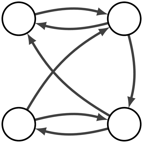
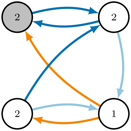
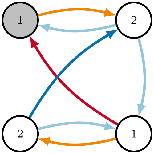
For local changes, we consider modifications to the latent group structure, allowing for any nN𝑛𝑁n\leq N nodes to change their group membership at any time tsuperscript𝑡t^{\prime}. In contrast to the approach of Matias and Miele (2017), in which the membership of node i𝑖i over the observation window behaves according to a discrete-time, irreducible and aperiodic Markov chain, we place no model on how or when nodes change and allow for any (finite) number of changes in a given interval. Furthermore, we allow for changes in continuous time, again in contrast to the discrete-time formulation of Matias and Miele (2017). Our main objective is only to detect if and when nodes have changed memberships, not to estimate the underlying group membership switching process. Figure 3 illustrates the effect of a single node switch in the case of N=4𝑁4N=4 nodes.

Refer to caption
(a) Observed graph structure
Refer to caption
(b) Latent group structure
Refer to caption
(c) Change in latent group structure
Figure 3: Visualisation of an observed graph 𝒢𝒢\mathcal{G} with N=4𝑁4N=4, with a change in the latent group structure. The changing node is coloured in grey, and edges are coloured according to the groups they connect.

For global changes, we consider jumps in the intensity between any groups k,m𝒦𝑘𝑚𝒦k,m\in\mathcal{K} at some time t+superscript𝑡subscriptt^{\prime}\in\mathbb{R}_{+} of the form λkmλkmmaps-tosubscript𝜆𝑘𝑚superscriptsubscript𝜆𝑘𝑚\lambda_{km}\mapsto\lambda_{km}^{\prime} (λkmλkmsubscript𝜆𝑘𝑚superscriptsubscript𝜆𝑘𝑚\lambda_{km}\neq\lambda_{km}^{\prime}). Again, we are interested in assessing if the block-specific intensity λkmsubscript𝜆𝑘𝑚\lambda_{km} has changed, and we do not estimate or posit assumptions on the mechanism that leads to such changes.

3 An online variational Bayesian estimation procedure

We present an online inference procedure for tracking the time-evolving latent structure and parameters of the BHPP model described in Section 2.1. We focus first on the set-up where the full edge set \mathcal{E} and the number of latent groups K𝐾K is known, as in Fang et al. (2024). Next, we consider when \mathcal{E} is unknown, and then we move to the case of an unknown number of groups, using a Bayesian nonparametric approach.

3.1 Variational Bayesian approximation

Variational Bayesian (VB) inference has the objective to approximate a posterior distribution when it is not analytically tractable (Wang and Blei, 2019), offering a faster estimation approach when compared to Markov Chain Monte Carlo methods (Blei et al., 2017). This makes it more suited to the requirements of an online learning framework. We adopt the terminology of Blei et al. (2017) in distinguishing between local latent variables z1,,zNsubscript𝑧1subscript𝑧𝑁z_{1},\dots,z_{N}, that scale with the number of nodes, and global latent variables θ=(π,λ)𝜃𝜋𝜆\theta=(\pi,\lambda), whose dimension, written S𝑆S\in\mathbb{N}, does not change with N𝑁N.

In a variational approach, one posits a family of distributions N+Ssuperscript𝑁𝑆\mathcal{F}^{N+S} on the parameter space (θ,z)𝜃𝑧(\theta,z), and seeks to select the component q(θ,z)N+Ssuperscript𝑞𝜃𝑧superscript𝑁𝑆q^{\ast}(\theta,z)\in\mathcal{F}^{N+S} closest to the true posterior p(θ,zx)𝑝𝜃conditional𝑧𝑥p(\theta,z\mid x) in the sense of the Kullback-Leibler (KL) divergence, where x𝑥x denotes the observed data. A mathematically convenient choice for N+Ssuperscript𝑁𝑆\mathcal{F}^{N+S} is the mean-field variational family, the set of factorisable distributions of the form

N+S={q:q(θ,z)=i=1Nqzi(zi)s=1Sqθs(θs)}.superscript𝑁𝑆conditional-set𝑞𝑞𝜃𝑧superscriptsubscriptproduct𝑖1𝑁subscript𝑞subscript𝑧𝑖subscript𝑧𝑖superscriptsubscriptproduct𝑠1𝑆subscript𝑞subscript𝜃𝑠subscript𝜃𝑠\mathcal{F}^{N+S}=\left\{q:q(\theta,z)=\prod_{i=1}^{N}q_{z_{i}}(z_{i})\prod_{s=1}^{S}q_{\theta_{s}}(\theta_{s})\right\}. (3.1)

The approximating distribution q(θ,z)N+Ssuperscript𝑞𝜃𝑧superscript𝑁𝑆q^{*}(\theta,z)\in\mathcal{F}^{N+S} is then given as

q(θ,z)=argminqN+SKL[q(θ,z)p(θ,z|x)].q^{\ast}(\theta,z)=\operatorname*{argmin}_{q\in\mathcal{F}^{N+S}}\mathrm{KL}\left[q(\theta,z)\ \|\ p(\theta,z|x)\right]. (3.2)

Despite every q(θ,z)N+S𝑞𝜃𝑧superscript𝑁𝑆q(\theta,z)\in\mathcal{F}^{N+S} taking a simple product structure, the solution q(θ,z)superscript𝑞𝜃𝑧q^{\ast}(\theta,z) to (3.2) is usually not available analytically. A popular method for approximating the global minimum q(θ,z)superscript𝑞𝜃𝑧q^{\ast}(\theta,z) of the KL-divergence is the Coordinate Ascent Variational Inference (CAVI) algorithm (Bishop, 2006; Blei et al., 2017), which iteratively updates each component of q(θ,z)𝑞𝜃𝑧q(\theta,z) while keeping the others fixed. Letting ϕitalic-ϕ\phi denote the (N+S)𝑁𝑆(N+S)-dimensional vector of latent variables ϕ=(z,θ)italic-ϕ𝑧𝜃\phi=(z,\theta), CAVI proceeds as follows:

q^ϕj(t+1)(ϕj)=argminqϕjKL[qϕj(ϕj)i<jq^ϕi(t+1)(ϕi)i>jq^ϕi(t)(ϕi)||p(ϕ|x)],\hat{q}_{\phi_{j}}^{(t+1)}(\phi_{j})=\operatorname*{argmin}_{q_{\phi_{j}}}\mathrm{KL}\left[q_{\phi_{j}}(\phi_{j})\prod_{i<j}\hat{q}_{\phi_{i}}^{(t+1)}(\phi_{i})\prod_{i>j}\hat{q}_{\phi_{i}}^{(t)}(\phi_{i})\ \Bigg{|}\Bigg{|}\ p(\phi|x)\right], (3.3)

for j{1,,N+S},t=0,1,2,formulae-sequence𝑗1𝑁𝑆𝑡012j\in\{1,\dots,N+S\},\ t=0,1,2,\dots until some convergence criterion is met. Under the mean-field variational approximation, (3.3) has the following solution (Bishop, 2006):

q^ϕjexp{𝔼ϕj[logp(x,ϕ)]},proportional-tosubscript^𝑞subscriptitalic-ϕ𝑗subscript𝔼subscriptitalic-ϕ𝑗delimited-[]𝑝𝑥italic-ϕ\hat{q}_{\phi_{j}}\propto\exp\{\mathbb{E}_{-\phi_{j}}\left[\log p(x,\phi)\right]\}, (3.4)

where the notation 𝔼ϕjsubscript𝔼subscriptitalic-ϕ𝑗\mathbb{E}_{-\phi_{j}} used to denote the expectation with respect to all components of ϕitalic-ϕ\phi except ϕjsubscriptitalic-ϕ𝑗\phi_{j} (Blei et al., 2017). As per convention with variational inference algorithms, we will drop the subscript on qϕj(ϕj)subscript𝑞subscriptitalic-ϕ𝑗subscriptitalic-ϕ𝑗q_{\phi_{j}}(\phi_{j}) for notational convenience, and take the argument of the variational component to index it (see, for example, Blei et al., 2017).

It should be noted that CAVI is only guaranteed to achieve a local minimum, and hence is sensitive to intialisation (Zhang and Zhou, 2020; Blei et al., 2017). Furthermore, with ϕ=(z,θ)italic-ϕ𝑧𝜃\phi=(z,\theta), updates in (3.4) have an explicit ordering. The ordering of the updates can also have implications on the convergence properties of the algorithm (Ray and Szabó, 2022), similarly to Gibbs sampling (see, for example, van Dyk and Park, 2008).

3.2 Online VB for the dynamic BHPP

Upon receiving the latest batch 𝒟rsubscript𝒟𝑟\mathcal{D}_{r} at time Lrsubscript𝐿𝑟L_{r}, the aim of the online algorithm is to update the estimates of the BHPP parameters based on the entire history 𝒟1:rsubscript𝒟:1𝑟\mathcal{D}_{1:r} of the process. To ensure finite and constant complexity and memory, a truly online algorithm should be single pass (see, for example Bifet et al., 2018): each data batch should be inspected only once, and summaries of previous data batches 𝒟1:(r1)subscript𝒟:1𝑟1\mathcal{D}_{1:(r-1)} are used in conjunction with 𝒟rsubscript𝒟𝑟\mathcal{D}_{r} to update parameter estimates.

The prior-posterior distribution updates within a Bayesian framework offers a natural way to propagate information forward in time. The posterior distribution at time Lr1subscript𝐿𝑟1L_{r-1} contains the information that was learned from 𝒟1:(r1)subscript𝒟:1𝑟1\mathcal{D}_{1:(r-1)}. A naive approach therefore is to pass this through as the new prior distribution for the update at time Lrsubscript𝐿𝑟L_{r}. However, this will perform poorly in the case of changing latent structure. As the number of batches increases, the new prior distributions become more concentrated around the current best estimates. This results in an updated posterior distribution that is largely dominated by its prior distribution (corresponding to the posterior distribution up to the previous batch) and which is increasingly insensitive to new data and changes in the data generating process.

We therefore propose to flatten the posterior obtained at Lr1subscript𝐿𝑟1L_{r-1}, via temperature parameters, at the point of passing it through as the prior distribution for the update at Lrsubscript𝐿𝑟L_{r}. This flattening step is in effect down-weighting previous observations and can therefore be considered as a Bayesian analogue of the forgetting factor procedure that has been widely used in frequentist online literature (see, for example, Haykin, 2002; Bodenham and Adams, 2017). In this way, the parameter estimates are quicker to respond to changes in the latent rate structure.

Due to the independence of counts from a Poisson process within non-overlapping time windows, the posterior density at step r𝑟r under the BHPP model factorises as

p(z,θ𝒟1:r)𝑝𝑧conditional𝜃subscript𝒟:1𝑟\displaystyle p(z,\theta\mid\mathcal{D}_{1:r}) =1rp(𝒟z,λ)×p(zπ)×p(π)×p(λ)p(𝒟rz,λ)×p(z,θ𝒟1:(r1)),proportional-toabsentsuperscriptsubscriptproduct1𝑟𝑝conditionalsubscript𝒟𝑧𝜆𝑝conditional𝑧𝜋𝑝𝜋𝑝𝜆proportional-to𝑝conditionalsubscript𝒟𝑟𝑧𝜆𝑝𝑧conditional𝜃subscript𝒟:1𝑟1\displaystyle\propto\prod_{\ell=1}^{r}p(\mathcal{D}_{\ell}\mid z,\lambda)\times p(z\mid\pi)\times p(\pi)\times p(\lambda)\propto p(\mathcal{D}_{r}\mid z,\lambda)\times p(z,\theta\mid\mathcal{D}_{1:(r-1)}), (3.5)

where the prior distributions are chosen to be conjugate, as per (2.3) and (2.5). From (3.5), the posterior distribution at step r1𝑟1r-1 can be interpreted as the prior for the posterior distribution at step r𝑟r.

The posterior density in (3.5) is not available in closed form and, due to the marginal density p(𝒟1:r)𝑝subscript𝒟:1𝑟p(\mathcal{D}_{1:r}) being unavailable, can only be evaluated up to a normalising constant. We thus consider the VB approach with the mean-field variational family, deploying the CAVI algorithm to compute approximate posterior distributions. Denoting the approximate posterior at step r1𝑟1r-1 by q^(r1)(θ,z)superscript^𝑞𝑟1𝜃𝑧\hat{q}^{(r-1)}(\theta,z), we pass through as the prior for step r𝑟r the tempered density

q^δ(r1)(θ,z)subscriptsuperscript^𝑞𝑟1𝛿𝜃𝑧\displaystyle\hat{q}^{(r-1)}_{\delta}(\theta,z) =k,m𝒦q^δλ(r1)(λkm)×i𝒱q^δz(r1)(zi)×q^δπ(r1)(π)absentsubscriptproduct𝑘𝑚𝒦subscriptsuperscript^𝑞𝑟1subscript𝛿𝜆subscript𝜆𝑘𝑚subscriptproduct𝑖𝒱subscriptsuperscript^𝑞𝑟1subscript𝛿𝑧subscript𝑧𝑖subscriptsuperscript^𝑞𝑟1subscript𝛿𝜋𝜋\displaystyle=\prod_{k,m\in\mathcal{K}}\hat{q}^{(r-1)}_{\delta_{\lambda}}(\lambda_{km})\times\prod_{i\in\mathcal{V}}\hat{q}^{(r-1)}_{\delta_{z}}(z_{i})\times\hat{q}^{(r-1)}_{\delta_{\pi}}(\pi) (3.6)
=1Cr1×k,m𝒦q^(r1)(λkm)δλ×i𝒱q^(r1)(zi)δz×q^(r1)(π)δπ,absent1subscript𝐶𝑟1subscriptproduct𝑘𝑚𝒦superscript^𝑞𝑟1superscriptsubscript𝜆𝑘𝑚subscript𝛿𝜆subscriptproduct𝑖𝒱superscript^𝑞𝑟1superscriptsubscript𝑧𝑖subscript𝛿𝑧superscript^𝑞𝑟1superscript𝜋subscript𝛿𝜋\displaystyle=\frac{1}{C_{r-1}}\times\prod_{k,m\in\mathcal{K}}\hat{q}^{(r-1)}(\lambda_{km})^{\delta_{\lambda}}\times\prod_{i\in\mathcal{V}}\hat{q}^{(r-1)}(z_{i})^{\delta_{z}}\times\hat{q}^{(r-1)}(\pi)^{\delta_{\pi}}, (3.7)

controlled by the Bayesian forgetting factor (BFF) δ=(δλ,δz,δπ)(0,1]3𝛿subscript𝛿𝜆subscript𝛿𝑧subscript𝛿𝜋superscript013\delta=(\delta_{\lambda},\delta_{z},\delta_{\pi})\in(0,1]^{3}. Here, Cr1subscript𝐶𝑟1C_{r-1} is a normalising constant to ensure a valid density. This procedure is visualised in Figure 4.

Refer to caption
Figure 4: A representation of the transformation of the CAVI approximation from the r𝑟r-th iteration via temperature parameters δ𝛿\delta and its use as a prior for the (r+1)𝑟1(r+1)-th iteration. The overlaying of 𝒟rsubscript𝒟𝑟\mathcal{D}_{r} on the diagonal arrows indicates that the transformed CAVI posterior is combined with incoming data to yield the next approximate posterior.

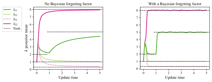
The effect of the BFF in down-weighting previous data and placing greater emphasis on the latest batch 𝒟rsubscript𝒟𝑟\mathcal{D}_{r} is illustrated in Figure 5. A fully-connected network is simulated on the time interval [0,5]05[0,5] with N=500𝑁500N=500 nodes and K=2𝐾2K=2 groups. An instantaneous rate change in λ11subscript𝜆11\lambda_{11} is made at t=1𝑡1t=1. The left panel of Figure 5 shows the results for naive approach (without a forgetting factor), whereas the right panel includes a BFF and demonstrates a much faster response to the change and quicker convergence of the posterior mean to the true value.
Refer to caption
Figure 5: Estimated posterior mean of λ+K×K𝜆superscriptsubscript𝐾𝐾\lambda\in\mathbb{R}_{+}^{K\times K} for a fully connected graph with N=500𝑁500N=500 nodes simulated on [0,5]05[0,5], with K=2𝐾2K=2 groups, π=(0.6,0.4)𝜋0.60.4\pi=(0.6,0.4), λ22=8,λ12=1,λ21=0.3formulae-sequencesubscript𝜆228formulae-sequencesubscript𝜆121subscript𝜆210.3\lambda_{22}=8,\ \lambda_{12}=1,\ \lambda_{21}=0.3, and λ11=2subscript𝜆112\lambda_{11}=2. At t=1𝑡1t=1, λ11subscript𝜆11\lambda_{11} changes to 555. The four coloured lines are the posterior means of the components λ𝜆\lambda, plotted against iteration. The black dashed horizontal lines are the true values of λ𝜆\lambda at each time point. δ=0.1𝛿0.1\delta=0.1 in the right-hand panel.

3.3 Online CAVI updates

We assume that each component of (3.6) takes the same form of its corresponding complete conditional distribution under the standard BHPP model in (2.2)–(2.5), raised to a power and normalised:

q^δλ(r1)(λkm)subscriptsuperscript^𝑞𝑟1subscript𝛿𝜆subscript𝜆𝑘𝑚\displaystyle\hat{q}^{(r-1)}_{\delta_{\lambda}}(\lambda_{km}) =1Cλkm,r1Gamma(αkm(r1),βkm(r1))δλ,absent1subscript𝐶subscript𝜆𝑘𝑚𝑟1Gammasuperscriptsuperscriptsubscript𝛼𝑘𝑚𝑟1superscriptsubscript𝛽𝑘𝑚𝑟1subscript𝛿𝜆\displaystyle=\frac{1}{C_{\lambda_{km},r-1}}\mathrm{Gamma}\left(\alpha_{km}^{(r-1)},\beta_{km}^{(r-1)}\right)^{\delta_{\lambda}}, k,m𝒦,𝑘𝑚𝒦\displaystyle k,m\in\mathcal{K},
q^δz(r1)(zi)subscriptsuperscript^𝑞𝑟1subscript𝛿𝑧subscript𝑧𝑖\displaystyle\hat{q}^{(r-1)}_{\delta_{z}}(z_{i}) =1Czi,r1Categorical(τ(r1))δz,absent1subscript𝐶subscript𝑧𝑖𝑟1Categoricalsuperscriptsuperscript𝜏𝑟1subscript𝛿𝑧\displaystyle=\frac{1}{C_{z_{i},r-1}}\mathrm{Categorical}\left(\tau^{(r-1)}\right)^{\delta_{z}}, i𝒱,𝑖𝒱\displaystyle i\in\mathcal{V},
q^δπ(r1)(π)subscriptsuperscript^𝑞𝑟1subscript𝛿𝜋𝜋\displaystyle\hat{q}^{(r-1)}_{\delta_{\pi}}(\pi) =1Cπ,r1Dirichlet(γ(r1))δπ.absent1subscript𝐶𝜋𝑟1Dirichletsuperscriptsuperscript𝛾𝑟1subscript𝛿𝜋\displaystyle=\frac{1}{C_{\pi,r-1}}\mathrm{Dirichlet}\left(\gamma^{(r-1)}\right)^{\delta_{\pi}}.

Here, Cλkm,r1,Czi,r1subscript𝐶subscript𝜆𝑘𝑚𝑟1subscript𝐶subscript𝑧𝑖𝑟1C_{\lambda_{km},r-1},C_{z_{i},r-1} and Cπ,r1subscript𝐶𝜋𝑟1C_{\pi,r-1} are normalising constants, ensuring that the densities are valid, and δ=(δλ,δz,δπ)(0,1]3𝛿subscript𝛿𝜆subscript𝛿𝑧subscript𝛿𝜋superscript013\delta=(\delta_{\lambda},\delta_{z},\delta_{\pi})\in(0,1]^{3} are temperature parameters specific to each class of latent variables. Suppose that data is observed on the interval Ir:=(Lr1,Lr]assignsubscript𝐼𝑟subscript𝐿𝑟1subscript𝐿𝑟I_{r}:=(L_{r-1},L_{r}], for r𝑟r\in\mathbb{N}, and denote the count on edge (i,j)𝑖𝑗(i,j) during this interval by xij(Ir)subscript𝑥𝑖𝑗subscript𝐼𝑟x_{ij}(I_{r}). Under the prior structure in (3.6), it is shown in Appendix A that the CAVI sequential updates are:

  1. 1.

    q^(r)(λkm)=Gamma(αkm(r),βkm(r))superscript^𝑞𝑟subscript𝜆𝑘𝑚Gammasubscriptsuperscript𝛼𝑟𝑘𝑚subscriptsuperscript𝛽𝑟𝑘𝑚\hat{q}^{(r)}(\lambda_{km})=\mathrm{Gamma}\left(\alpha^{(r)}_{km},\beta^{(r)}_{km}\right) for all k,m𝒦𝑘𝑚𝒦k,m\in\mathcal{K} where αkm(r),βkm(r)subscriptsuperscript𝛼𝑟𝑘𝑚subscriptsuperscript𝛽𝑟𝑘𝑚\alpha^{(r)}_{km},\beta^{(r)}_{km} are defined as:

    αkm(r)subscriptsuperscript𝛼𝑟𝑘𝑚\displaystyle\alpha^{(r)}_{km} =δλ(αkm(r1)1)+(i,j)τik(r1)τjm(r1)xij(Ir)+1,absentsubscript𝛿𝜆subscriptsuperscript𝛼𝑟1𝑘𝑚1subscript𝑖𝑗superscriptsubscript𝜏𝑖𝑘𝑟1superscriptsubscript𝜏𝑗𝑚𝑟1subscript𝑥𝑖𝑗subscript𝐼𝑟1\displaystyle=\delta_{\lambda}\left(\alpha^{(r-1)}_{km}-1\right)+\sum_{(i,j)\in\mathcal{E}}\tau_{ik}^{(r-1)}\tau_{jm}^{(r-1)}x_{ij}(I_{r})+1, (3.8)
    βkm(r)subscriptsuperscript𝛽𝑟𝑘𝑚\displaystyle\beta^{(r)}_{km} =δλβkm(r1)+Δ(i,j)τik(r1)τjm(r1).absentsubscript𝛿𝜆subscriptsuperscript𝛽𝑟1𝑘𝑚Δsubscript𝑖𝑗superscriptsubscript𝜏𝑖𝑘𝑟1superscriptsubscript𝜏𝑗𝑚𝑟1\displaystyle=\delta_{\lambda}\beta^{(r-1)}_{km}+\Delta\sum_{(i,j)\in\mathcal{E}}\tau_{ik}^{(r-1)}\tau_{jm}^{(r-1)}. (3.9)
  2. 2.

    q^(r)(zi)=Categorical(τi(r))superscript^𝑞𝑟subscript𝑧𝑖Categoricalsuperscriptsubscript𝜏𝑖𝑟\hat{q}^{(r)}(z_{i})=\mathrm{Categorical}\left(\tau_{i}^{(r)}\right) for all i𝒱𝑖𝒱i\in\mathcal{V} where τi(r)=(τi1(r),,τiK(r))superscriptsubscript𝜏𝑖𝑟superscriptsubscript𝜏𝑖1𝑟superscriptsubscript𝜏𝑖𝐾𝑟\tau_{i}^{(r)}=(\tau_{i1}^{(r)},\dots,\tau_{iK}^{(r)}), with k𝒦τik(r)=1subscript𝑘𝒦superscriptsubscript𝜏𝑖𝑘𝑟1\sum_{k\in\mathcal{K}}\tau_{ik}^{(r)}=1, satisfies the relation:

    τik(r)superscriptsubscript𝜏𝑖𝑘𝑟\displaystyle\tau_{ik}^{(r)} exp{δz[ψ(γk(r1))ψ(m𝒦γm(r1))]+xii(Ir)[ψ(αkk(r))log(βkk(r))]Δαkk(r)βkk(r)+\displaystyle\propto\exp\Bigg{\{}\delta_{z}\left[\psi\left(\gamma^{(r-1)}_{k}\right)-\psi\left(\sum_{m\in\mathcal{K}}\gamma^{(r-1)}_{m}\right)\right]\ +x_{ii}(I_{r})\left[\psi\left(\alpha_{kk}^{(r)}\right)-\log\left(\beta_{kk}^{(r)}\right)\right]-\Delta\frac{\alpha_{kk}^{(r)}}{\beta_{kk}^{(r)}}+
    m𝒦[j:(i,j)τjm(r)(xij(Ir){ψ(αkm(r))log(βkm(r))}Δαkm(r)βkm(r))(1𝕀{k}(m)𝕀{i}(j))+\displaystyle\sum_{m\in\mathcal{K}}\Bigg{[}\sum_{j:(i,j)\in\mathcal{E}}\tau_{jm}^{(r)}\bigg{(}x_{ij}(I_{r})\left\{\psi\left(\alpha^{(r)}_{km}\right)-\log\left(\beta^{(r)}_{km}\right)\right\}-\Delta\frac{\alpha^{(r)}_{km}}{\beta^{(r)}_{km}}\bigg{)}\bigg{(}1-\mathbb{I}_{\{k\}}(m)\mathbb{I}_{\{i\}}(j)\bigg{)}\ +
    j:(j,i)τjm(r)(xji(Ir){ψ(αmk(r))log(βmk(r))}Δαmk(r)βmk(r))(1𝕀{k}(m)𝕀{i}(j))]}.\displaystyle\sum_{j^{\prime}:(j^{\prime},i)\in\mathcal{E}}\tau_{j^{\prime}m}^{(r)}\bigg{(}x_{j^{\prime}i}(I_{r})\left\{\psi\left(\alpha^{(r)}_{mk}\right)-\log\left(\beta^{(r)}_{mk}\right)\right\}-\Delta\frac{\alpha^{(r)}_{mk}}{\beta^{(r)}_{mk}}\bigg{)}\bigg{(}1-\mathbb{I}_{\{k\}}(m)\mathbb{I}_{\{i\}}(j^{\prime})\bigg{)}\Bigg{]}\Bigg{\}}. (3.10)
  3. 3.

    q^(r)(π)=Dirichlet{(γ1(r),,γK(r))}superscript^𝑞𝑟𝜋Dirichletsubscriptsuperscript𝛾𝑟1subscriptsuperscript𝛾𝑟𝐾\hat{q}^{(r)}(\pi)=\mathrm{Dirichlet}\left\{\left(\gamma^{(r)}_{1},\dots,\gamma^{(r)}_{K}\right)\right\} where γk(r)subscriptsuperscript𝛾𝑟𝑘\gamma^{(r)}_{k} is defined as:

    γk(r)=δπ(γk(r1)1)+δzi𝒱τik(r)+1.subscriptsuperscript𝛾𝑟𝑘subscript𝛿𝜋superscriptsubscript𝛾𝑘𝑟11subscript𝛿𝑧subscript𝑖𝒱superscriptsubscript𝜏𝑖𝑘𝑟1\displaystyle\gamma^{(r)}_{k}=\delta_{\pi}\left(\gamma_{k}^{(r-1)}-1\right)+\delta_{z}\sum_{i\in\mathcal{V}}\tau_{ik}^{(r)}+1. (3.11)

Here ψ()𝜓\psi(\cdot) is the digamma function. Note that the parameters τik(r),i𝒱,k𝒦formulae-sequencesuperscriptsubscript𝜏𝑖𝑘𝑟𝑖𝒱𝑘𝒦\tau_{ik}^{(r)},\ i\in\mathcal{V},\ k\in\mathcal{K}, are jointly optimised via a fixed point solver for (3.10), iteratively moving through the rows of the matrix τ={τik}i𝒱,k𝒦[0,1]N×K𝜏subscriptsubscript𝜏𝑖𝑘formulae-sequence𝑖𝒱𝑘𝒦superscript01𝑁𝐾\tau=\{\tau_{ik}\}_{i\in\mathcal{V},\ k\in\mathcal{K}}\in[0,1]^{N\times K} until convergence. The fixed point solver is initialised at the r𝑟r-th step by using the value of τ𝜏\tau outputted from the (r1)𝑟1(r-1)-th step as the starting point, which also partially circumvents the problem of label switching (Jasra et al., 2005).

Algorithm 1 describes the full inference procedure based upon the updates in equations (3.9)–(3.11).

Algorithm 1 Online VB Procedure for BHPP
Initialise α(0)superscript𝛼0\alpha^{(0)}, β(0)superscript𝛽0\beta^{(0)}, γ(0)superscript𝛾0\gamma^{(0)} and set τik=1/Ksubscript𝜏𝑖𝑘1𝐾\tau_{ik}=1/K for all i𝒱𝑖𝒱i\in\mathcal{V} and k𝒦𝑘𝒦k\in\mathcal{K}.
for r=1,2,𝑟12r=1,2,\dots do
     for =1,2,,NCAVI12subscript𝑁CAVI\ell=1,2,\dots,N_{\mathrm{CAVI}} do
         while τ𝜏\tau not converged do
              for j=1𝑗1j=1 to N𝑁N do
                  Update τj=(τj1,,τjK)subscript𝜏𝑗subscript𝜏𝑗1subscript𝜏𝑗𝐾\tau_{j}=(\tau_{j1},\dots,\tau_{jK}) as in equation (3.10), intialising as the output of update r1𝑟1r-1.
              end for
         end while
         Normalise τisubscript𝜏𝑖\tau_{i} such that k=1Kτik=1superscriptsubscript𝑘1𝐾subscript𝜏𝑖𝑘1\sum_{k=1}^{K}\tau_{ik}=1.
         Update γ(r)superscript𝛾𝑟\gamma^{(r)}, α(r)superscript𝛼𝑟\alpha^{(r)} and β(r)superscript𝛽𝑟\beta^{(r)} as in (3.9)–(3.11).
     end for
end for

3.4 Detecting changepoints

In this work, we aim to detect two types of changepoints: changes in the point process rates and changes in the group memberships.

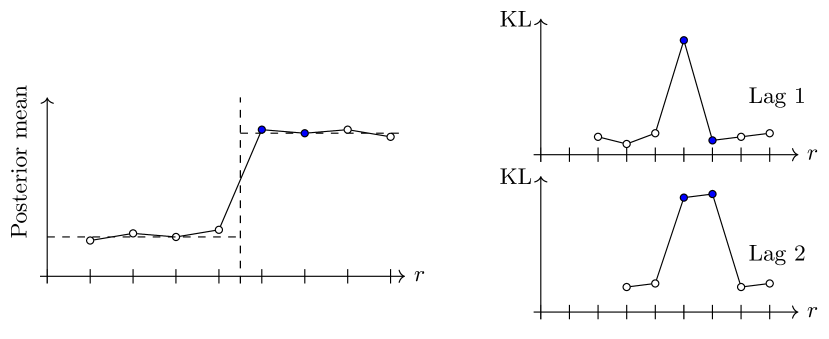
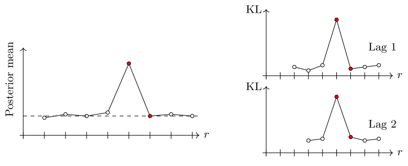
To detect changes in the point process rates, we compute the KL-divergence between the approximate posteriors q^(r)(λkm)superscript^𝑞𝑟subscript𝜆𝑘𝑚\hat{q}^{(r)}(\lambda_{km}) and q^(rs)(λkm)superscript^𝑞𝑟𝑠subscript𝜆𝑘𝑚\hat{q}^{(r-s)}(\lambda_{km}), for s=1,2,,κ𝑠12𝜅s=1,2,\dots,\kappa, where κ𝜅\kappa\in\mathbb{N} is a lag parameter. We compare the current approximation with estimates beyond that of the previous update, up to a maximal lag of κ𝜅\kappa, to avoid incorrectly flagging outliers as changes. Figure 6(a) illustrates the behaviour of the KL-divergence for a lag of 1 and a lag of 2. In Figure 6(b), we see that using only a lag of 1 would result in the false identification of a change. There is a trade-off to be made between confidence and speed of detection. We found that a maximal lag of κ=2𝜅2\kappa=2 provided a good balance.

To compute the KL-divergence, we note that q^(r)(λkm)superscript^𝑞𝑟subscript𝜆𝑘𝑚\hat{q}^{(r)}(\lambda_{km}) is gamma distributed for all r𝑟r\in\mathbb{N}. For two random variables X1Gamma(α1,β1)similar-tosubscript𝑋1Gammasubscript𝛼1subscript𝛽1X_{1}\sim\mathrm{Gamma}(\alpha_{1},\beta_{1}) and X2Gamma(α2,β2)similar-tosubscript𝑋2Gammasubscript𝛼2subscript𝛽2X_{2}\sim\mathrm{Gamma}(\alpha_{2},\beta_{2}) with probability distributions p1subscript𝑝1p_{1} and p2subscript𝑝2p_{2} respectively, their KL-divergence is:

KL(p1p2)=α2logβ1β2logΓ(α1)Γ(α2)+(α1α2)ψ(α1)(β1β2)α1β1.KLconditionalsubscript𝑝1subscript𝑝2subscript𝛼2subscript𝛽1subscript𝛽2Γsubscript𝛼1Γsubscript𝛼2subscript𝛼1subscript𝛼2𝜓subscript𝛼1subscript𝛽1subscript𝛽2subscript𝛼1subscript𝛽1\mathrm{KL}(p_{1}\ \|\ p_{2})=\alpha_{2}\log\frac{\beta_{1}}{\beta_{2}}-\log\frac{\Gamma(\alpha_{1})}{\Gamma(\alpha_{2})}+(\alpha_{1}-\alpha_{2})\psi(\alpha_{1})-(\beta_{1}-\beta_{2})\frac{\alpha_{1}}{\beta_{1}}. (3.12)

Two burn-in times are required to make use of the KL-divergence. In particular, B1subscript𝐵1B_{1}\in\mathbb{N} iterations are needed for the algorithm to converge from initialisation, and B2subscript𝐵2B_{2}\in\mathbb{N} further steps needed to obtain enough samples to flag changes. During the initial B1+B2subscript𝐵1subscript𝐵2B_{1}+B_{2} steps, stationarity is assumed. After B1+B2subscript𝐵1subscript𝐵2B_{1}+B_{2} steps, we propose to use the median absolute deviation (MAD) to evaluate the presence of a changepoint, as it is robust to outliers (Leys et al., 2013). In general, for a dataset 𝒴:={yi}i=1nassign𝒴superscriptsubscriptsubscript𝑦𝑖𝑖1𝑛\mathcal{Y}:=\{y_{i}\}_{i=1}^{n}, the MAD is defined as

MAD=med({|yimed(𝒴)|}i=1n),MADmedsuperscriptsubscriptsubscript𝑦𝑖med𝒴𝑖1𝑛\mathrm{MAD}=\operatorname*{med}\big{(}\{|y_{i}-\operatorname*{med}(\mathcal{Y})|\}_{i=1}^{n}\big{)}, (3.13)

where med()med\operatorname*{med}(\cdot) denotes the median of the elements in a set. An observation yj𝒴subscript𝑦𝑗𝒴y_{j}\in\mathcal{Y} is classified as an outlier if |yjmed(𝒴)|>LMADsubscript𝑦𝑗med𝒴𝐿MAD|y_{j}-\operatorname*{med}(\mathcal{Y})|>L\cdot\mathrm{MAD}, for a choice of threshold L+𝐿subscriptL\in\mathbb{R}_{+}.

In our proposed methodology, the elements in the set 𝒴𝒴\mathcal{Y} are the realised values of the KL-divergence between different gamma distributions, approximating the posterior distributions for the parameters λkm,k,m𝒦subscript𝜆𝑘𝑚𝑘𝑚𝒦\lambda_{km},\ k,m\in\mathcal{K} at different time windows. In particular, we write ykmr,s:=KL[q(r)(λkm)q(rs)(λkm)]assignsubscriptsuperscript𝑦𝑟𝑠𝑘𝑚KLdelimited-[]conditionalsuperscript𝑞𝑟subscript𝜆𝑘𝑚superscript𝑞𝑟𝑠subscript𝜆𝑘𝑚y^{r,s}_{km}:=\mathrm{KL}[q^{(r)}(\lambda_{km})\ \|\ q^{(r-s)}(\lambda_{km})] and construct 𝒴kms:={ykmr,s}rB1+B2+sassignsuperscriptsubscript𝒴𝑘𝑚𝑠subscriptsubscriptsuperscript𝑦𝑟𝑠𝑘𝑚𝑟subscript𝐵1subscript𝐵2𝑠\mathcal{Y}_{km}^{s}:=\{y^{r,s}_{km}\}_{r\geq B_{1}+B_{2}+s}. A changepoint is flagged at t=rΔ𝑡𝑟Δt=r\Delta if for all s=1,2,,κ𝑠12𝜅s=1,2,\dots,\kappa, we have:

|ykmr+s1,smed(𝒴kms)|>LMAD.superscriptsubscript𝑦𝑘𝑚𝑟𝑠1𝑠medsuperscriptsubscript𝒴𝑘𝑚𝑠𝐿MAD|y_{km}^{r+s-1,s}-\operatorname*{med}(\mathcal{Y}_{km}^{s})|>L\cdot\mathrm{MAD}. (3.14)

It must be remarked that if we choose a maximal lag of κ𝜅\kappa, we can only flag a changepoint a minimum of κ1𝜅1\kappa-1 time steps after the changepoint has occurred.

We now consider whether the stream must be reset post change. Suppose a change to the latent rate λ𝜆\lambda occurs at some time Lr<t<Lr+1subscript𝐿𝑟superscript𝑡subscript𝐿𝑟1L_{r}<t^{\prime}<L_{r+1}, and that pre-change λGamma(α,β)similar-to𝜆Gamma𝛼𝛽\lambda\sim\mathrm{Gamma}(\alpha,\beta), whereas λGamma(α,β)similar-to𝜆Gammasuperscript𝛼superscript𝛽\lambda\sim\mathrm{Gamma}(\alpha^{\prime},\beta^{\prime}) post-change, for αα𝛼superscript𝛼\alpha\neq\alpha^{\prime} and ββ𝛽superscript𝛽\beta\neq\beta^{\prime}. Pre-change, our algorithm provides two consecutive CAVI estimates q(r1)(λ)superscript𝑞𝑟1𝜆q^{(r-1)}(\lambda) and q(r)(λ)superscript𝑞𝑟𝜆q^{(r)}(\lambda), with shapes and rates α(r1),β(r1)superscript𝛼𝑟1superscript𝛽𝑟1\alpha^{(r-1)},\beta^{(r-1)} and α(r),β(r)superscript𝛼𝑟superscript𝛽𝑟\alpha^{(r)},\beta^{(r)}, respectively, and post-change, we have CAVI estimates q(r+1)(λ)superscript𝑞𝑟1𝜆q^{(r+1)}(\lambda) and q(r+2)(λ)superscript𝑞𝑟2𝜆q^{(r+2)}(\lambda) with shapes and rates α(r+1),β(r+1)superscript𝛼𝑟1superscript𝛽𝑟1\alpha^{(r+1)},\beta^{(r+1)} and α(r+2),β(r+2)superscript𝛼𝑟2superscript𝛽𝑟2\alpha^{(r+2)},\beta^{(r+2)}. For ease of analysis, we suppose that α(r)α(r1)=α(r+2)α(r+1)=Δαsuperscript𝛼𝑟superscript𝛼𝑟1superscript𝛼𝑟2superscript𝛼𝑟1subscriptΔ𝛼\alpha^{(r)}-\alpha^{(r-1)}=\alpha^{(r+2)}-\alpha^{(r+1)}=\Delta_{\alpha}, and β(r)β(r1)=β(r+2)β(r+1)=Δβsuperscript𝛽𝑟superscript𝛽𝑟1superscript𝛽𝑟2superscript𝛽𝑟1subscriptΔ𝛽\beta^{(r)}-\beta^{(r-1)}=\beta^{(r+2)}-\beta^{(r+1)}=\Delta_{\beta}.

We consider the ratio of the KL-divergences between consecutive estimates pre and post-change, and expand as Δα0subscriptΔ𝛼0\Delta_{\alpha}\to 0 to get

KL(q(r+2)q(r+1))KL(q(r)q(r1))=α(r+1)(Δβ/β(r+1)log(1+Δβ/β(r+1)))α(r1)(Δβ/β(r1)log(1+Δβ/β(r1)))+𝒪(Δα).KLconditionalsuperscript𝑞𝑟2superscript𝑞𝑟1KLconditionalsuperscript𝑞𝑟superscript𝑞𝑟1superscript𝛼𝑟1subscriptΔ𝛽superscript𝛽𝑟11subscriptΔ𝛽superscript𝛽𝑟1superscript𝛼𝑟1subscriptΔ𝛽superscript𝛽𝑟11subscriptΔ𝛽superscript𝛽𝑟1𝒪subscriptΔ𝛼\frac{\mathrm{KL}(q^{(r+2)}\ \|\ q^{(r+1)})}{\mathrm{KL}(q^{(r)}\ \|\ q^{(r-1)})}=\frac{\alpha^{(r+1)}\left(\Delta_{\beta}/\beta^{(r+1)}-\log\left(1+\Delta_{\beta}/\beta^{(r+1)}\right)\right)}{\alpha^{(r-1)}\left(\Delta_{\beta}/\beta^{(r-1)}-\log\left(1+\Delta_{\beta}/\beta^{(r-1)}\right)\right)}+\mathcal{O}(\Delta_{\alpha}). (3.15)

Similarly, taking Δβ0subscriptΔ𝛽0\Delta_{\beta}\to 0 yields

KL(q(r+2)q(r+1))KL(q(r)q(r1))=log{Γ(α(r+1))/Γ(α(r+1)+Δα)}+Δαψ(α(r+1))log{Γ(α(r1))/Γ(α(r1)+Δα)}+Δαψ(α(r1))+𝒪(Δβ).KLconditionalsuperscript𝑞𝑟2superscript𝑞𝑟1KLconditionalsuperscript𝑞𝑟superscript𝑞𝑟1Γsuperscript𝛼𝑟1Γsuperscript𝛼𝑟1subscriptΔ𝛼subscriptΔ𝛼𝜓superscript𝛼𝑟1Γsuperscript𝛼𝑟1Γsuperscript𝛼𝑟1subscriptΔ𝛼subscriptΔ𝛼𝜓superscript𝛼𝑟1𝒪subscriptΔ𝛽\frac{\mathrm{KL}(q^{(r+2)}\ \|\ q^{(r+1)})}{\mathrm{KL}(q^{(r)}\ \|\ q^{(r-1)})}=\frac{\log\left\{\Gamma(\alpha^{(r+1)})/\Gamma(\alpha^{(r+1)}+\Delta_{\alpha})\right\}+\Delta_{\alpha}\psi(\alpha^{(r+1)})}{\log\left\{\Gamma(\alpha^{(r-1)})/\Gamma(\alpha^{(r-1)}+\Delta_{\alpha})\right\}+\Delta_{\alpha}\psi(\alpha^{(r-1)})}+\mathcal{O}(\Delta_{\beta}). (3.16)

Observation of (3.15) indicates that to first order the ratio depends upon only the relative size of the difference between their rates, that is Δβ/βsubscriptΔ𝛽𝛽\Delta_{\beta}/\beta, and not directly upon the magnitude of β𝛽\beta. This is not problematic only if the magnitude of ΔβsubscriptΔ𝛽\Delta_{\beta} changes linearly with β𝛽\beta. Also, (3.16) shows that the ratio depends directly on the magnitude of the scale α𝛼\alpha. It follows that after the identification of a changepoint at t=rcΔ𝑡subscript𝑟𝑐Δt=r_{c}\Delta, rcsubscript𝑟𝑐r_{c}\in\mathbb{N}, the stream of realised KL-divergence values must be discarded, and the algorithm wait a further B2subscript𝐵2B_{2} steps to obtain enough samples for the new set 𝒴kms:={ykmr,s}rrc+B2+sassignsuperscriptsubscript𝒴𝑘𝑚𝑠subscriptsuperscriptsubscript𝑦𝑘𝑚𝑟𝑠𝑟subscript𝑟𝑐subscript𝐵2𝑠\mathcal{Y}_{km}^{s}:=\{y_{km}^{r,s}\}_{r\geq r_{c}+B_{2}+s} which is used to detect any subsequent changes. A further benefit of consider a maximal lag κ>1𝜅1\kappa>1 is that more KL-divergence samples are obtained for the same number of observations.

To detect changes in the group memberships, the approximation i𝒱q^(zi)subscriptproduct𝑖𝒱^𝑞subscript𝑧𝑖\prod_{i\in\mathcal{V}}\hat{q}(z_{i}) to the posterior of the latent group memberships in (3.10) provides a node-level vector τisubscript𝜏𝑖\tau_{i} (i=1,,N)i=1,...,N) of group membership probabilities. Computing argmaxkτiksubscriptargmax𝑘subscript𝜏𝑖𝑘\operatorname*{argmax}_{k}\tau_{ik} provides a group assignment for node i𝑖i, and by comparing assignments between runs, one has a natural way of flagging changes. However, this approach is unsatisfactory as it does not account for the magnitude of the change in probability. The KL-divergence also cannot be used for flagging group changes, since KL(p1p2)KLconditionalsubscript𝑝1subscript𝑝2\mathrm{KL}(p_{1}\ \|\ p_{2}) is only defined only when p2>0subscript𝑝20p_{2}>0 for all values in the support of p1subscript𝑝1p_{1}. Instead, we utilise the Jensen-Shannon divergence (JS; Lin, 1991), defined for two distributions p1,p2subscript𝑝1subscript𝑝2p_{1},p_{2} as

JS(p1p2)=12KL(p1p)+12KL(p2p),JSconditionalsubscript𝑝1subscript𝑝212KLconditionalsubscript𝑝1𝑝12KLconditionalsubscript𝑝2𝑝\mathrm{JS}(p_{1}\ \|\ p_{2})=\frac{1}{2}\mathrm{KL}(p_{1}\ \|\ p)+\frac{1}{2}\mathrm{KL}(p_{2}\ \|\ p), (3.17)

where p:=(p1+p2)/2assign𝑝subscript𝑝1subscript𝑝22p:=(p_{1}+p_{2})/2 is a 50-50 mixture distribution of p1subscript𝑝1p_{1} and p2subscript𝑝2p_{2}. The JS-divergence is symmetric in its arguments, and avoids the undefined values encountered with the KL-divergence. For q1,q2Δnsubscript𝑞1subscript𝑞2superscriptΔ𝑛q_{1},q_{2}\in\Delta^{n}, where ΔnsuperscriptΔ𝑛\Delta^{n} denotes the n𝑛n-dimensional simplex, the JS-divergence between discrete random variables X1Categorical(q1)similar-tosubscript𝑋1Categoricalsubscript𝑞1X_{1}\sim\mathrm{Categorical}(q_{1}) and X2Categorical(q2)similar-tosubscript𝑋2Categoricalsubscript𝑞2X_{2}\sim\mathrm{Categorical}(q_{2}), with probability mass functions p1subscript𝑝1p_{1} and p2subscript𝑝2p_{2} respectively, takes the following form:

JS(p1p2)=12(i=1nq1ilogq1i(q1i+q2i)/2+i=1nq2ilogq2i(q1i+q2i)/2).JSconditionalsubscript𝑝1subscript𝑝212superscriptsubscript𝑖1𝑛subscript𝑞1𝑖subscript𝑞1𝑖subscript𝑞1𝑖subscript𝑞2𝑖2superscriptsubscript𝑖1𝑛subscript𝑞2𝑖subscript𝑞2𝑖subscript𝑞1𝑖subscript𝑞2𝑖2\mathrm{JS}(p_{1}\ \|\ p_{2})=\frac{1}{2}\left(\sum_{i=1}^{n}q_{1i}\log\frac{q_{1i}}{(q_{1i}+q_{2i})/2}+\sum_{i=1}^{n}q_{2i}\log\frac{q_{2i}}{(q_{1i}+q_{2i})/2}\right). (3.18)

The MAD is then used to detect changes to the stream of logged values, but with two additional requirements on the group probabilities:

argmaxkτik(r)argmaxkτik(rs),subscriptargmax𝑘subscriptsuperscript𝜏𝑟𝑖𝑘subscriptargmax𝑘subscriptsuperscript𝜏𝑟𝑠𝑖𝑘\displaystyle\operatorname*{argmax}_{k}\tau^{(r)}_{ik}\neq\operatorname*{argmax}_{k}\tau^{(r-s)}_{ik}, for all s=1,,κ,for all 𝑠1𝜅\displaystyle\text{for all }s=1,\dots,\kappa, (3.19)
argmaxkτik(rs1)=argmaxkτik(rs2),subscriptargmax𝑘subscriptsuperscript𝜏𝑟subscript𝑠1𝑖𝑘subscriptargmax𝑘subscriptsuperscript𝜏𝑟subscript𝑠2𝑖𝑘\displaystyle\operatorname*{argmax}_{k}\tau^{(r-s_{1})}_{ik}=\operatorname*{argmax}_{k}\tau^{(r-s_{2})}_{ik}, for all s1,s2{1,,κ}.for all subscript𝑠1subscript𝑠21𝜅\displaystyle\text{for all }s_{1},s_{2}\in\{1,\dots,\kappa\}. (3.20)

If the MAD condition and both (3.19) and (3.20) are met, then a changepoint is flagged. The conditions (3.19) and (3.20) ensure that changes are flagged only if the most likely group assignment changes after a window of κ𝜅\kappa steps where the most likely group assignment was stable. It should noted that for this stream, as the probabilities are constrained to sum to 1, we do not reset these values after a changepoint is detected.
Refer to caption
(a) A true changepoint.
Refer to caption
(b) An outlier.
Figure 6: Illustration of the behaviour of the KL-divergence with different lags for a changepoint and an outlier.


3.5 Online VB for the dynamic BHPP with an unknown underlying graph

Until now, it has been assumed that the graph is fully connected. We relax this assumption and extend the framework to the setting where 𝑨={aij}{0,1}N×N𝑨subscript𝑎𝑖𝑗superscript01𝑁𝑁\bm{A}=\{a_{ij}\}\in\{0,1\}^{N\times N} is unknown. Assuming aij=1subscript𝑎𝑖𝑗1a_{ij}=1 when there is no edge adversely affects estimation of the latent rates; instead of the absence of an event indicating the absence of an edge, it instead just leads to a lower rate estimate. This motivates a method that can take into account the possibility that aij=0subscript𝑎𝑖𝑗0a_{ij}=0. The work here builds upon the sparse setup of Matias et al. (2018).

For each (i,j)𝑖𝑗(i,j)\in\mathcal{R}, an additional latent variable aij{0,1}subscript𝑎𝑖𝑗01a_{ij}\in\{0,1\} is introduced. A new latent group membership zi𝒦:={1,,K}superscriptsubscript𝑧𝑖superscript𝒦assign1superscript𝐾z_{i}^{\prime}\in\mathcal{K}^{\prime}:=\{1,\dots,K^{\prime}\} is assigned to each i𝒱𝑖𝒱i\in\mathcal{V}, and aijsubscript𝑎𝑖𝑗a_{ij} is Bernoulli-distributed conditional upon zisuperscriptsubscript𝑧𝑖z_{i}^{\prime} and zjsuperscriptsubscript𝑧𝑗z_{j}^{\prime}, according to a stochastic blockmodel (SBM; Holland et al., 1983). Each aijsubscript𝑎𝑖𝑗a_{ij} captures the probability that (i,j)𝑖𝑗(i,j)\in\mathcal{R} is also an element of \mathcal{E}, and functions to reduce the contribution of edges with no arrivals to the estimates of the underlying rates. The new model is then expressed as:

xij(t)aij,zi,zj,λzizjconditionalsubscript𝑥𝑖𝑗𝑡subscript𝑎𝑖𝑗subscript𝑧𝑖subscript𝑧𝑗subscript𝜆subscript𝑧𝑖subscript𝑧𝑗\displaystyle x_{ij}(t)\mid a_{ij},z_{i},z_{j},\lambda_{z_{i}z_{j}} Poisson(aijλzizjt),similar-toabsentPoissonsubscript𝑎𝑖𝑗subscript𝜆subscript𝑧𝑖subscript𝑧𝑗𝑡\displaystyle\sim\mathrm{Poisson}(a_{ij}\lambda_{z_{i}z_{j}}t), for all i,j𝒱,for all 𝑖𝑗𝒱\displaystyle\text{for all }i,j\in\mathcal{V}, (3.21)
λkmsubscript𝜆𝑘𝑚\displaystyle\lambda_{km} Gamma(αkm0,βkm0),similar-toabsentGammasuperscriptsubscript𝛼𝑘𝑚0superscriptsubscript𝛽𝑘𝑚0\displaystyle\sim\mathrm{Gamma}\left(\alpha_{km}^{0},\beta_{km}^{0}\right), for all k,m𝒦,for all 𝑘𝑚𝒦\displaystyle\text{for all }k,m\in\mathcal{K}, (3.22)
aijzi,zj,ρzizjconditionalsubscript𝑎𝑖𝑗superscriptsubscript𝑧𝑖superscriptsubscript𝑧𝑗subscript𝜌superscriptsubscript𝑧𝑖superscriptsubscript𝑧𝑗\displaystyle a_{ij}\mid z_{i}^{\prime},z_{j}^{\prime},\rho_{z_{i}^{\prime}z_{j}^{\prime}} Bernoulli(ρzizj),similar-toabsentBernoullisubscript𝜌superscriptsubscript𝑧𝑖superscriptsubscript𝑧𝑗\displaystyle\sim\mathrm{Bernoulli}(\rho_{z_{i}^{\prime}z_{j}^{\prime}}), for all i,j𝒱,for all 𝑖𝑗𝒱\displaystyle\text{for all }i,j\in\mathcal{V}, (3.23)
ρkmsubscript𝜌superscript𝑘superscript𝑚\displaystyle\rho_{k^{\prime}m^{\prime}} Beta(ηkm0,ζkm0),similar-toabsentBetasuperscriptsubscript𝜂superscript𝑘superscript𝑚0superscriptsubscript𝜁superscript𝑘superscript𝑚0\displaystyle\sim\mathrm{Beta}\left(\eta_{k^{\prime}m^{\prime}}^{0},\zeta_{k^{\prime}m^{\prime}}^{0}\right), for all k,m𝒦,for all superscript𝑘superscript𝑚superscript𝒦\displaystyle\text{for all }k^{\prime},m^{\prime}\in\mathcal{K}^{\prime}, (3.24)
ziπconditionalsubscript𝑧𝑖𝜋\displaystyle z_{i}\mid\pi Categorical(π),similar-toabsentCategorical𝜋\displaystyle\sim\mathrm{Categorical}(\pi), for all i𝒱,for all 𝑖𝒱\displaystyle\text{for all }i\in\mathcal{V}, (3.25)
ziμconditionalsuperscriptsubscript𝑧𝑖𝜇\displaystyle z_{i}^{\prime}\mid\mu Categorical(μ),similar-toabsentCategorical𝜇\displaystyle\sim\mathrm{Categorical}(\mu), for all i𝒱,for all 𝑖𝒱\displaystyle\text{for all }i\in\mathcal{V}, (3.26)
π𝜋\displaystyle\pi Dirichlet(γ0),similar-toabsentDirichletsuperscript𝛾0\displaystyle\sim\mathrm{Dirichlet}\left(\gamma^{0}\right), (3.27)
μ𝜇\displaystyle\mu Dirichlet(ξ0),similar-toabsentDirichletsuperscript𝜉0\displaystyle\sim\mathrm{Dirichlet}\left(\xi^{0}\right), (3.28)

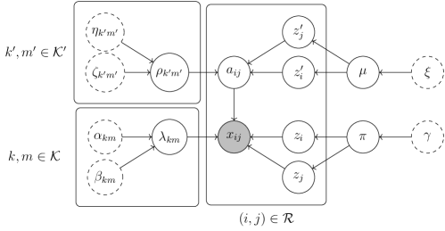
We allow the most general setting in which the group structure that governs the rates is separate from that which determines edge connection probabilities. We assume that the graph is static, and so changes to the memberships that drive the edge-processes should not affect the determination of the graph adjacency matrix. The decoupling of the edge-process and edge-connection group memberships ensure this. Furthermore, as has been noted, SBMs provide good approximations to any exchangeable random graph model (Airoldi et al., 2013), and they therefore offer a logical model for the graph generation mechanism. This new model structure is represented in graphical model form in Figure 7.
Refer to caption
Figure 7: A directed acyclic graphical model representation of the model in (3.21)-(3.28).

Given the graph is considered to be static, if xij(t)>0subscript𝑥𝑖𝑗𝑡0x_{ij}(t)>0 for some t𝑡t, then (i,j)𝑖𝑗(i,j)\in\mathcal{E} (corresponding to aij=1subscript𝑎𝑖𝑗1a_{ij}=1) with probability one. Otherwise, if xij(t)=0subscript𝑥𝑖𝑗𝑡0x_{ij}(t)=0 then we either have no edge (corresponding to aij=0subscript𝑎𝑖𝑗0a_{i}j=0), or a non-null intensity process with no events in (0,t]0𝑡(0,t]. The difference with the Section 2.1 is that we now have the additional local latent variables, z𝑧z, zsuperscript𝑧z^{\prime} and 𝑨𝑨\bm{A}, all of which grow with N𝑁N (linearly for z𝑧z and zsuperscript𝑧z^{\prime}, and quadratically for 𝑨𝑨\bm{A}).

To implement variational inference, the full conditional distribution p(aijzi,zj,zi,zj,λzizj,ρzizj,𝒟1:r)𝑝conditionalsubscript𝑎𝑖𝑗subscript𝑧𝑖subscript𝑧𝑗superscriptsubscript𝑧𝑖superscriptsubscript𝑧𝑗subscript𝜆subscript𝑧𝑖subscript𝑧𝑗subscript𝜌superscriptsubscript𝑧𝑖superscriptsubscript𝑧𝑗subscript𝒟:1𝑟p(a_{ij}\mid z_{i},z_{j},z_{i}^{\prime},z_{j}^{\prime},\lambda_{z_{i}z_{j}},\rho_{z_{i}^{\prime}z_{j}^{\prime}},\mathcal{D}_{1:r}) must be written down exactly, as per (3.4). Using the fact that inter-arrival times from a Poisson process are exponentially distributed, Matias et al. (2018) shows that the conditional posterior probability of an edge (i,j)𝑖𝑗(i,j)\in\mathcal{E} in the case of static λ𝜆\lambda takes the form

p(aij=1𝒟1:r,zi=k,zj=m,zi=k,zj=m,λkm,ρkm)=𝕀{xij(rΔ)>0}+𝕀{xij(rΔ)=0}ρkmexp(λkmrΔ)1ρkm+ρkmexp(λkmrΔ).p(a_{ij}=1\mid\mathcal{D}_{1:r},z_{i}=k,z_{j}=m,z_{i}^{\prime}=k^{\prime},z_{j}^{\prime}=m^{\prime},\lambda_{km},\rho_{k^{\prime}m^{\prime}})=\\ \mathbb{I}\{x_{ij}(r\Delta)>0\}+\frac{\mathbb{I}\{x_{ij}(r\Delta)=0\}\rho_{k^{\prime}m^{\prime}}\exp\left(-\lambda_{km}r\Delta\right)}{1-\rho_{k^{\prime}m^{\prime}}+\rho_{k^{\prime}m^{\prime}}\exp\left(-\lambda_{km}r\Delta\right)}. (3.29)

Since 𝑨𝑨\bm{A} is static, the posterior for each aijsubscript𝑎𝑖𝑗a_{ij} should be computed using the full data 𝒟1:rsubscript𝒟:1𝑟\mathcal{D}_{1:r}. Note that the conditional distribution in  (3.29) depends on 𝒟1:rsubscript𝒟:1𝑟\mathcal{D}_{1:r} only via the counting process xij()subscript𝑥𝑖𝑗x_{ij}(\cdot) at time rΔ𝑟Δr\Delta.

For the model in (3.21)-(3.28), the true posterior distribution after r𝑟r batches factorises as

p(𝑨,z,z,θ𝒟1:r)𝑝𝑨𝑧superscript𝑧conditional𝜃subscript𝒟:1𝑟\displaystyle p(\bm{A},z,z^{\prime},\theta\mid\mathcal{D}_{1:r}) p(𝒟r𝑨,z,zθ)×p(𝑨,z,z,θ𝒟1:(r1)),proportional-toabsent𝑝conditionalsubscript𝒟𝑟𝑨𝑧superscript𝑧𝜃𝑝𝑨𝑧superscript𝑧conditional𝜃subscript𝒟:1𝑟1\displaystyle\propto p(\mathcal{D}_{r}\mid\bm{A},z,z^{\prime}\theta)\times p(\bm{A},z,z^{\prime},\theta\mid\mathcal{D}_{1:(r-1)}), (3.30)

similarly to the posterior distribution in (3.5). Therefore, inference on this model can be performed in much the same way as inference on the original model. However, as the true conditional posterior for 𝑨𝑨\bm{A} is tractable, the update procedure is slightly different. Unlike Matias et al. (2018), we cannot simply take q(r)(aij)superscript𝑞𝑟subscript𝑎𝑖𝑗q^{(r)}(a_{ij}) to be Bernoulli distributed with probability as in (3.29) as λ𝜆\lambda is, in general, not static. Instead, to account for variations in λ𝜆\lambda over the full observation window, we propose an approximation to the posterior distribution of aijsubscript𝑎𝑖𝑗a_{ij} at t=rΔ𝑡𝑟Δt=r\Delta, conditional upon zi=k,zj=m,zi=k,zj=mformulae-sequencesubscript𝑧𝑖𝑘formulae-sequencesubscript𝑧𝑗𝑚formulae-sequencesuperscriptsubscript𝑧𝑖superscript𝑘superscriptsubscript𝑧𝑗superscript𝑚z_{i}=k,z_{j}=m,z_{i}^{\prime}=k^{\prime},z_{j}^{\prime}=m^{\prime}, of the form q^(r)(aij)=Bernoulli(σij(r))superscript^𝑞𝑟subscript𝑎𝑖𝑗Bernoullisuperscriptsubscript𝜎𝑖𝑗𝑟\hat{q}^{(r)}(a_{ij})=\mathrm{Bernoulli}\left(\sigma_{ij}^{(r)}\right), where

σij(r)=𝕀{xij(rΔ)>0}+𝕀{xij(rΔ)=0}ρ^km(r)exp(Δ=0rλ^km())1ρ^km(r)+ρ^km(r)exp(Δ=0rλ^km()).superscriptsubscript𝜎𝑖𝑗𝑟𝕀subscript𝑥𝑖𝑗𝑟Δ0𝕀subscript𝑥𝑖𝑗𝑟Δ0superscriptsubscript^𝜌superscript𝑘superscript𝑚𝑟Δsuperscriptsubscript0𝑟subscriptsuperscript^𝜆𝑘𝑚1superscriptsubscript^𝜌superscript𝑘superscript𝑚𝑟superscriptsubscript^𝜌superscript𝑘superscript𝑚𝑟Δsuperscriptsubscript0𝑟subscriptsuperscript^𝜆𝑘𝑚\sigma_{ij}^{(r)}=\mathbb{I}\{x_{ij}(r\Delta)>0\}+\frac{\mathbb{I}\{x_{ij}(r\Delta)=0\}\hat{\rho}_{k^{\prime}m^{\prime}}^{(r)}\exp\left(-\Delta\sum_{\ell=0}^{r}\hat{\lambda}^{(\ell)}_{km}\right)}{1-\hat{\rho}_{k^{\prime}m^{\prime}}^{(r)}+\hat{\rho}_{k^{\prime}m^{\prime}}^{(r)}\exp\left(-\Delta\sum_{\ell=0}^{r}\hat{\lambda}^{(\ell)}_{km}\right)}. (3.31)

Here, ρ^km()superscriptsubscript^𝜌superscript𝑘superscript𝑚\hat{\rho}_{k^{\prime}m^{\prime}}^{(\ell)} and λ^km()superscriptsubscript^𝜆𝑘𝑚\hat{\lambda}_{km}^{(\ell)} denote the mean of our approximate posterior distribution for ρkm()superscriptsubscript𝜌superscript𝑘superscript𝑚\rho_{k^{\prime}m^{\prime}}^{(\ell)} and λkm()superscriptsubscript𝜆𝑘𝑚\lambda_{km}^{(\ell)}, respectively, at update \ell. At update r𝑟r, we propose a variational approximation of the form q(r)(𝑨,z,z,θ)=(i,j)Bernoulli(σij(r))×q(θ,z,z)superscript𝑞𝑟𝑨𝑧superscript𝑧𝜃subscriptproduct𝑖𝑗Bernoullisuperscriptsubscript𝜎𝑖𝑗𝑟𝑞𝜃𝑧superscript𝑧q^{(r)}(\bm{A},z,z^{\prime},\theta)=\prod_{(i,j)\in\mathcal{R}}\mathrm{Bernoulli}(\sigma_{ij}^{(r)})\times q(\theta,z,z^{\prime}), where σij(r)superscriptsubscript𝜎𝑖𝑗𝑟\sigma_{ij}^{(r)} is as in (3.31) and q(θ,z,z)2N+S𝑞𝜃𝑧superscript𝑧superscript2𝑁𝑆q(\theta,z,z^{\prime})\in\mathcal{F}^{2N+S}. A two-step estimation procedure follows naturally, wherein q(θ,z,z)𝑞𝜃𝑧superscript𝑧q(\theta,z,z^{\prime}) is approximated using CAVI as was done previously, and then σij(r)subscriptsuperscript𝜎𝑟𝑖𝑗\sigma^{(r)}_{ij} is updated using (3.31) and the CAVI approximations to the posteriors of λ𝜆\lambda and ρ𝜌\rho. Note that since aijsubscript𝑎𝑖𝑗a_{ij} for i,j𝒱𝑖𝑗𝒱i,j\in\mathcal{V}, zisuperscriptsubscript𝑧𝑖z_{i}^{\prime} for i𝒱𝑖𝒱i\in\mathcal{V}, ρkmsubscript𝜌superscript𝑘superscript𝑚\rho_{k^{\prime}m^{\prime}} for k,m𝒦superscript𝑘superscript𝑚superscript𝒦k^{\prime},m^{\prime}\in\mathcal{K}^{\prime} and μ𝜇\mu are considered static parameters, forgetting factors for these quantities are not required.

Consider the BHPP model with unknown graph structure, as in (3.21)-(3.28), with global parameters θ=(λ,π,μ,ρ)𝜃𝜆𝜋𝜇𝜌\theta=(\lambda,\pi,\mu,\rho) and local parameters z𝑧z, zsuperscript𝑧z^{\prime} and 𝑨𝑨\bm{A}. At step r1𝑟1r-1, we approximate the posterior density p(𝑨,z,z,θ𝒟1:(r1))𝑝𝑨𝑧superscript𝑧conditional𝜃subscript𝒟:1𝑟1p(\bm{A},z,z^{\prime},\theta\mid\mathcal{D}_{1:(r-1)}) by q^(r1)(𝑨,z,z,θ)superscript^𝑞𝑟1𝑨𝑧superscript𝑧𝜃\hat{q}^{(r-1)}(\bm{A},z,z^{\prime},\theta), which is the product of the optimal CAVI solution q^(r1)(z,z,θ)superscript^𝑞𝑟1𝑧superscript𝑧𝜃\hat{q}^{(r-1)}(z,z^{\prime},\theta) and the fixed-form approximation q^(r1)(𝑨)superscript^𝑞𝑟1𝑨\hat{q}^{(r-1)}(\bm{A}) of (3.31). For the BHPP model with known graph structure, all latent variables could change, and thus in (3.7) all components were tempered before being passed as the prior for step r𝑟r. However, in the case of an unknown graph structure, as the graph is assumed to be static, only the components of the dynamic latent variables are tempered when constructing the prior for step r𝑟r. We pass through as the prior for step r𝑟r the partially tempered density

q^δ(r1)(𝑨,z,θ)=subscriptsuperscript^𝑞𝑟1𝛿𝑨𝑧𝜃absent\displaystyle\hat{q}^{(r-1)}_{\delta}(\bm{A},z,\theta)= k,m𝒦q^(r1)(ρkm)×i𝒱q^(r1)(zi)×(i,j)q^(r1)(aij)×q^(r1)(μ)×\displaystyle\prod_{k,m\in\mathcal{K}}\hat{q}^{(r-1)}(\rho_{km})\times\prod_{i\in\mathcal{V}}\hat{q}^{(r-1)}(z_{i}^{\prime})\times\prod_{(i,j)\in\mathcal{R}}\hat{q}^{(r-1)}(a_{ij})\times\hat{q}^{(r-1)}(\mu)\times (3.32)
i𝒱q^δz(r1)(zi)×k,m𝒦q^δλ(r1)(λkm)×q^δπ(r1)(π).subscriptproduct𝑖𝒱subscriptsuperscript^𝑞𝑟1subscript𝛿𝑧subscript𝑧𝑖subscriptproduct𝑘𝑚𝒦subscriptsuperscript^𝑞𝑟1subscript𝛿𝜆subscript𝜆𝑘𝑚subscriptsuperscript^𝑞𝑟1subscript𝛿𝜋𝜋\displaystyle\prod_{i\in\mathcal{V}}\hat{q}^{(r-1)}_{\delta_{z}}(z_{i})\times\prod_{k,m\in\mathcal{K}}\hat{q}^{(r-1)}_{\delta_{\lambda}}(\lambda_{km})\times\hat{q}^{(r-1)}_{\delta_{\pi}}(\pi). (3.33)

We assume that each component of (3.33) takes the same form as its corresponding complete conditional distribution under the BHPP model with unknown graph structure of (3.21)-(3.28). Additionally, the distributions for λ𝜆\lambda, π𝜋\pi and z𝑧z are raised to a power and normalised. In summary:

q^(r1)(aij)superscript^𝑞𝑟1subscript𝑎𝑖𝑗\displaystyle\hat{q}^{(r-1)}(a_{ij}) =Bernoulli(σij(r1)),absentBernoullisuperscriptsubscript𝜎𝑖𝑗𝑟1\displaystyle=\mathrm{Bernoulli}\left(\sigma_{ij}^{{(r-1)}}\right), i,j𝒱,𝑖𝑗𝒱\displaystyle i,j\in\mathcal{V},
q^δλ(r1)(λkm)subscriptsuperscript^𝑞𝑟1subscript𝛿𝜆subscript𝜆𝑘𝑚\displaystyle\hat{q}^{(r-1)}_{\delta_{\lambda}}(\lambda_{km}) =1Cλkm,r1Gamma(αkm(r1),βkm(r1))δλ,absent1subscript𝐶subscript𝜆𝑘𝑚𝑟1Gammasuperscriptsuperscriptsubscript𝛼𝑘𝑚𝑟1superscriptsubscript𝛽𝑘𝑚𝑟1subscript𝛿𝜆\displaystyle=\frac{1}{C_{\lambda_{km},r-1}}\mathrm{Gamma}\left(\alpha_{km}^{(r-1)},\beta_{km}^{(r-1)}\right)^{\delta_{\lambda}}, k,m𝒦,𝑘𝑚𝒦\displaystyle k,m\in\mathcal{K},
q^(r1)(ρkm)superscript^𝑞𝑟1subscript𝜌superscript𝑘superscript𝑚\displaystyle\hat{q}^{(r-1)}(\rho_{k^{\prime}m^{\prime}}) =Beta(ηkm(r1),ζkm(r1)),absentBetasubscriptsuperscript𝜂𝑟1superscript𝑘superscript𝑚subscriptsuperscript𝜁𝑟1superscript𝑘superscript𝑚\displaystyle=\mathrm{Beta}\left(\eta^{(r-1)}_{k^{\prime}m^{\prime}},\zeta^{(r-1)}_{k^{\prime}m^{\prime}}\right), k,m𝒦,superscript𝑘superscript𝑚superscript𝒦\displaystyle k^{\prime},m^{\prime}\in\mathcal{K}^{\prime},
q^(r1)(zi)superscript^𝑞𝑟1subscript𝑧𝑖\displaystyle\hat{q}^{(r-1)}(z_{i}) =1Czi,r1Categorical(τi(r1))δz,absent1subscript𝐶subscript𝑧𝑖𝑟1Categoricalsuperscriptsuperscriptsubscript𝜏𝑖𝑟1subscript𝛿𝑧\displaystyle=\frac{1}{C_{z_{i},r-1}}\mathrm{Categorical}\left(\tau_{i}^{(r-1)}\right)^{\delta_{z}}, i𝒱,𝑖𝒱\displaystyle i\in\mathcal{V},
q^(r1)(zi)superscript^𝑞𝑟1superscriptsubscript𝑧𝑖\displaystyle\hat{q}^{(r-1)}(z_{i}^{\prime}) =Categorical(νi(r1)),absentCategoricalsuperscriptsubscript𝜈𝑖𝑟1\displaystyle=\mathrm{Categorical}\left(\nu_{i}^{(r-1)}\right), i𝒱,𝑖𝒱\displaystyle i\in\mathcal{V},
q^δπ(r1)(π)subscriptsuperscript^𝑞𝑟1subscript𝛿𝜋𝜋\displaystyle\hat{q}^{(r-1)}_{\delta_{\pi}}(\pi) =1Cπ,r1Dirichlet(γ(r1))δπ,absent1subscript𝐶𝜋𝑟1Dirichletsuperscriptsuperscript𝛾𝑟1subscript𝛿𝜋\displaystyle=\frac{1}{C_{\pi,r-1}}\mathrm{Dirichlet}\left(\gamma^{(r-1)}\right)^{\delta_{\pi}},
q^(r1)(μ)superscript^𝑞𝑟1𝜇\displaystyle\hat{q}^{(r-1)}(\mu) =Dirichlet(ξ(r1)).absentDirichletsuperscript𝜉𝑟1\displaystyle=\mathrm{Dirichlet}\left(\xi^{(r-1)}\right).

Suppose that data is again observed on the interval Ir:=(Lr1,Lr]assignsubscript𝐼𝑟subscript𝐿𝑟1subscript𝐿𝑟I_{r}:=(L_{r-1},L_{r}], for r𝑟r\in\mathbb{N}. Under the prior structure in (3.33), the CAVI sequential updates take the form:

  1. 1.

    q^(r)(λkm)=Gamma(αkm(r),βkm(r))superscript^𝑞𝑟subscript𝜆𝑘𝑚Gammasuperscriptsubscript𝛼𝑘𝑚𝑟superscriptsubscript𝛽𝑘𝑚𝑟\hat{q}^{(r)}(\lambda_{km})=\mathrm{Gamma}\left(\alpha_{km}^{(r)},\beta_{km}^{(r)}\right) where for all k,m𝒦𝑘𝑚𝒦k,m\in\mathcal{K} we define αkm(r)superscriptsubscript𝛼𝑘𝑚𝑟\alpha_{km}^{(r)} and βkm(r)superscriptsubscript𝛽𝑘𝑚𝑟\beta_{km}^{(r)} as

    αkm(r)superscriptsubscript𝛼𝑘𝑚𝑟\displaystyle\alpha_{km}^{(r)} =δλ(αkm(r1)1)+(i,j)τik(r1)τjm(r1)σij(r1)xij(r)+1,absentsubscript𝛿𝜆subscriptsuperscript𝛼𝑟1𝑘𝑚1subscript𝑖𝑗subscriptsuperscript𝜏𝑟1𝑖𝑘subscriptsuperscript𝜏𝑟1𝑗𝑚superscriptsubscript𝜎𝑖𝑗𝑟1superscriptsubscript𝑥𝑖𝑗𝑟1\displaystyle=\delta_{\lambda}\left(\alpha^{(r-1)}_{km}-1\right)+\sum_{(i,j)\in\mathcal{R}}\tau^{(r-1)}_{ik}\tau^{(r-1)}_{jm}\sigma_{ij}^{(r-1)}x_{ij}^{(r)}+1, (3.34)
    βkm(r)superscriptsubscript𝛽𝑘𝑚𝑟\displaystyle\beta_{km}^{(r)} =δλβkm(r1)+(i,j)τik(r1)τjm(r1)σij(r1).absentsubscript𝛿𝜆subscriptsuperscript𝛽𝑟1𝑘𝑚subscript𝑖𝑗subscriptsuperscript𝜏𝑟1𝑖𝑘subscriptsuperscript𝜏𝑟1𝑗𝑚superscriptsubscript𝜎𝑖𝑗𝑟1\displaystyle=\delta_{\lambda}\beta^{(r-1)}_{km}+\sum_{(i,j)\in\mathcal{R}}\tau^{(r-1)}_{ik}\tau^{(r-1)}_{jm}\sigma_{ij}^{(r-1)}. (3.35)
  2. 2.

    q^(r)(ρkm)=Beta(ηkm(r),ζkm(r))superscript^𝑞𝑟subscript𝜌superscript𝑘superscript𝑚Betasubscriptsuperscript𝜂𝑟superscript𝑘superscript𝑚subscriptsuperscript𝜁𝑟superscript𝑘superscript𝑚\hat{q}^{(r)}(\rho_{k^{\prime}m^{\prime}})=\mathrm{Beta}\left(\eta^{(r)}_{k^{\prime}m^{\prime}},\zeta^{(r)}_{k^{\prime}m^{\prime}}\right) where for all k,m𝒦superscript𝑘superscript𝑚superscript𝒦k^{\prime},m^{\prime}\in\mathcal{K}^{\prime}, we define ηkm(r)superscriptsubscript𝜂superscript𝑘superscript𝑚𝑟\eta_{k^{\prime}m^{\prime}}^{(r)} and ζkm(r)superscriptsubscript𝜁superscript𝑘superscript𝑚𝑟\zeta_{k^{\prime}m^{\prime}}^{(r)} as

    ηkm(r)superscriptsubscript𝜂superscript𝑘superscript𝑚𝑟\displaystyle\eta_{k^{\prime}m^{\prime}}^{(r)} =ηkm(r1)+(i,j)νik(r1)νjm(r1)σij(r1)+1,absentsuperscriptsubscript𝜂superscript𝑘superscript𝑚𝑟1subscript𝑖𝑗subscriptsuperscript𝜈𝑟1𝑖superscript𝑘subscriptsuperscript𝜈𝑟1𝑗superscript𝑚superscriptsubscript𝜎𝑖𝑗𝑟11\displaystyle=\eta_{k^{\prime}m^{\prime}}^{(r-1)}+\sum_{(i,j)\in\mathcal{R}}\nu^{(r-1)}_{ik^{\prime}}\nu^{(r-1)}_{jm^{\prime}}\sigma_{ij}^{(r-1)}+1, (3.36)
    ζkm(r)superscriptsubscript𝜁superscript𝑘superscript𝑚𝑟\displaystyle\zeta_{k^{\prime}m^{\prime}}^{(r)} =ζkm(r1)+(i,j)νik(r1)νjm(r1)(1σij(r1)).absentsuperscriptsubscript𝜁superscript𝑘superscript𝑚𝑟1subscript𝑖𝑗subscriptsuperscript𝜈𝑟1𝑖superscript𝑘subscriptsuperscript𝜈𝑟1𝑗superscript𝑚1superscriptsubscript𝜎𝑖𝑗𝑟1\displaystyle=\zeta_{k^{\prime}m^{\prime}}^{(r-1)}+\sum_{(i,j)\in\mathcal{R}}\nu^{(r-1)}_{ik^{\prime}}\nu^{(r-1)}_{jm^{\prime}}\left(1-\sigma_{ij}^{(r-1)}\right).
  3. 3.

    q^(r)(zi)=Categorical(τi(r))superscript^𝑞𝑟subscript𝑧𝑖Categoricalsuperscriptsubscript𝜏𝑖𝑟\hat{q}^{(r)}(z_{i})=\mathrm{Categorical}\left(\tau_{i}^{(r)}\right) for all i𝒱𝑖𝒱i\in\mathcal{V} where τi(r)=(τi1(r),,τiK(r))superscriptsubscript𝜏𝑖𝑟superscriptsubscript𝜏𝑖1𝑟superscriptsubscript𝜏𝑖𝐾𝑟\tau_{i}^{(r)}=(\tau_{i1}^{(r)},\dots,\tau_{iK}^{(r)}), with k𝒦τik(r)=1subscript𝑘𝒦superscriptsubscript𝜏𝑖𝑘𝑟1\sum_{k\in\mathcal{K}}\tau_{ik}^{(r)}=1, satisfies the relation:

    τik(r)superscriptsubscript𝜏𝑖𝑘𝑟\displaystyle\tau_{ik}^{(r)} exp{δz[ψ(γk(r1))ψ(=1Kγ(r1))]+j𝒱m𝒦τjm(r)[Δ(σij(r1)αkm(r)βkm(r)+σji(r1)αmk(r)βmk(r))+\displaystyle\propto\exp\Bigg{\{}\delta_{z}\left[\psi\left(\gamma^{(r-1)}_{k}\right)-\psi\left(\sum_{\ell=1}^{K}\gamma^{(r-1)}_{\ell}\right)\right]+\sum_{j\in\mathcal{V}}\sum_{m\in\mathcal{K}}\tau_{jm}^{(r)}\Bigg{[}-\Delta\left(\sigma_{ij}^{(r-1)}\frac{\alpha^{(r)}_{km}}{\beta^{(r)}_{km}}+\sigma_{ji}^{(r-1)}\frac{\alpha^{(r)}_{mk}}{\beta^{(r)}_{mk}}\right)+
    xij(Ir)σij(r1)[ψ(αkm(r))log(βkm(r))]+xji(Ir)σji(r1)[ψ(αmk(r))log(βmk(r))]]×\displaystyle\qquad x_{ij}(I_{r})\ \sigma_{ij}^{(r-1)}\left[\psi\left(\alpha^{(r)}_{km}\right)-\log\left(\beta^{(r)}_{km}\right)\right]+x_{ji}(I_{r})\ \sigma_{ji}^{(r-1)}\left[\psi\left(\alpha^{(r)}_{mk}\right)-\log\left(\beta^{(r)}_{mk}\right)\right]\Bigg{]}\times (3.37)
    (1𝕀{i}(j)𝕀{k}(m))+σii(r1)[xii(Ir)[ψ(αkk(r))log(βkk(r))]Δαkkβkk]}.\displaystyle\qquad\bigg{(}1-\mathbb{I}_{\{i\}}(j)\mathbb{I}_{\{k\}}(m)\bigg{)}+\sigma_{ii}^{(r-1)}\bigg{[}x_{ii}(I_{r})\left[\psi\left(\alpha^{(r)}_{kk}\right)-\log\left(\beta^{(r)}_{kk}\right)\right]-\Delta\frac{\alpha_{kk}}{\beta_{kk}}\bigg{]}\Bigg{\}}. (3.38)
  4. 4.

    q^(r)(zi)=Categorical(νi(r))superscript^𝑞𝑟superscriptsubscript𝑧𝑖Categoricalsuperscriptsubscript𝜈𝑖𝑟\hat{q}^{(r)}(z_{i}^{\prime})=\mathrm{Categorical}\left(\nu_{i}^{(r)}\right) for all i𝒱𝑖𝒱i\in\mathcal{V} where νi(r)=(νi1(r),,νiK(r))superscriptsubscript𝜈𝑖𝑟superscriptsubscript𝜈𝑖1𝑟superscriptsubscript𝜈𝑖superscript𝐾𝑟\nu_{i}^{(r)}=(\nu_{i1}^{(r)},\dots,\nu_{iK^{\prime}}^{(r)}), with k𝒦νik(r)=1subscriptsuperscript𝑘superscript𝒦superscriptsubscript𝜈𝑖superscript𝑘𝑟1\sum_{k^{\prime}\in\mathcal{K}^{\prime}}\nu_{ik^{\prime}}^{(r)}=1, satisfies the relation:

    νik(r)superscriptsubscript𝜈𝑖superscript𝑘𝑟\displaystyle\nu_{ik^{\prime}}^{(r)} exp{ψ(ξk(r))ψ(=1Kξ(r))+j𝒱m𝒦νjm(r)[σij(r)[ψ(ηkm(r))ψ(ηkm(r)+ζkm(r))]+\displaystyle\propto\exp\Bigg{\{}\psi\left(\xi^{(r)}_{k^{\prime}}\right)-\psi\left(\sum_{\ell^{\prime}=1}^{K^{\prime}}\xi^{(r)}_{\ell^{\prime}}\right)+\sum_{j\in\mathcal{V}}\sum_{m^{\prime}\in\mathcal{K}^{\prime}}\nu_{jm^{\prime}}^{(r)}\Bigg{[}\sigma_{ij}^{(r)}\left[\psi\left(\eta^{(r)}_{k^{\prime}m^{\prime}}\right)-\psi\left(\eta^{(r)}_{k^{\prime}m^{\prime}}+\zeta^{(r)}_{k^{\prime}m^{\prime}}\right)\right]+
    (1σij(r))[ψ(ζkm(r))ψ(ζkm(r)+ηkm(r))]+σji(r)[ψ(ηmk(r))ψ(ηmk(r)+ζmk(r))]+1superscriptsubscript𝜎𝑖𝑗𝑟delimited-[]𝜓subscriptsuperscript𝜁𝑟superscript𝑘superscript𝑚𝜓superscriptsubscript𝜁superscript𝑘superscript𝑚𝑟superscriptsubscript𝜂superscript𝑘superscript𝑚𝑟limit-fromsuperscriptsubscript𝜎𝑗𝑖𝑟delimited-[]𝜓subscriptsuperscript𝜂𝑟superscript𝑚superscript𝑘𝜓subscriptsuperscript𝜂𝑟superscript𝑚superscript𝑘subscriptsuperscript𝜁𝑟superscript𝑚superscript𝑘\displaystyle\qquad\left(1-\sigma_{ij}^{(r)}\right)\left[\psi\left(\zeta^{(r)}_{k^{\prime}m^{\prime}}\right)-\psi\left(\zeta_{k^{\prime}m^{\prime}}^{(r)}+\eta_{k^{\prime}m^{\prime}}^{(r)}\right)\right]+\sigma_{ji}^{(r)}\left[\psi\left(\eta^{(r)}_{m^{\prime}k^{\prime}}\right)-\psi\left(\eta^{(r)}_{m^{\prime}k^{\prime}}+\zeta^{(r)}_{m^{\prime}k^{\prime}}\right)\right]+
    (1σji(r))[ψ(ζmk(r))ψ(ζmk(r)+ηmk(r))]](1𝕀{k}(m)𝕀{i}(j))+\displaystyle\qquad\left(1-\sigma_{ji}^{(r)}\right)\left[\psi\left(\zeta^{(r)}_{m^{\prime}k^{\prime}}\right)-\psi\left(\zeta_{m^{\prime}k^{\prime}}^{(r)}+\eta_{m^{\prime}k^{\prime}}^{(r)}\right)\right]\Bigg{]}\bigg{(}1-\mathbb{I}_{\{k^{\prime}\}}(m^{\prime})\mathbb{I}_{\{i\}}(j)\bigg{)}+ (3.39)
    σii(r)[ψ(ηkk(r))ψ(ηkk(r)+ζkk(r))]+(1σii(r))[ψ(ζkk(r))ψ(ηkk(r)+ζkk(r))]}.\displaystyle\qquad\sigma_{ii}^{(r)}\bigg{[}\psi\left(\eta^{(r)}_{k^{\prime}k^{\prime}}\right)-\psi\left(\eta^{(r)}_{k^{\prime}k^{\prime}}+\zeta^{(r)}_{k^{\prime}k^{\prime}}\right)\bigg{]}+\left(1-\sigma_{ii}^{(r)}\right)\bigg{[}\psi\left(\zeta^{(r)}_{k^{\prime}k^{\prime}}\right)-\psi\left(\eta^{(r)}_{k^{\prime}k^{\prime}}+\zeta^{(r)}_{k^{\prime}k^{\prime}}\right)\bigg{]}\Bigg{\}}. (3.40)
  5. 5.

    q^(r)(π)=Dirichlet(γ(r))superscript^𝑞𝑟𝜋Dirichletsuperscript𝛾𝑟\hat{q}^{(r)}(\pi)=\mathrm{Dirichlet}\left(\gamma^{(r)}\right) where for all k𝒦𝑘𝒦k\in\mathcal{K}, we define γk(r)subscriptsuperscript𝛾𝑟𝑘\gamma^{(r)}_{k} as:

    γk(r)=δπ(γk(r1)1)+δzi𝒱τik(r)+1,k𝒦.formulae-sequencesubscriptsuperscript𝛾𝑟𝑘subscript𝛿𝜋superscriptsubscript𝛾𝑘𝑟11subscript𝛿𝑧subscript𝑖𝒱subscriptsuperscript𝜏𝑟𝑖𝑘1𝑘𝒦\displaystyle\gamma^{(r)}_{k}=\delta_{\pi}\left(\gamma_{k}^{(r-1)}-1\right)+\delta_{z}\sum_{i\in\mathcal{V}}\tau^{(r)}_{ik}+1,\quad k\in\mathcal{K}. (3.41)
  6. 6.

    q^(r)(μ)=Dirichlet(ξ(r))superscript^𝑞𝑟𝜇Dirichletsuperscript𝜉𝑟\hat{q}^{(r)}(\mu)=\mathrm{Dirichlet}\left(\xi^{(r)}\right) where for all k𝒦superscript𝑘superscript𝒦k^{\prime}\in\mathcal{K}^{\prime}, we define ξk(r)superscriptsubscript𝜉superscript𝑘𝑟\xi_{k^{\prime}}^{(r)} as:

    ξk(r)=ξk(r1)+i𝒱νik(r),k𝒦.formulae-sequencesubscriptsuperscript𝜉𝑟superscript𝑘superscriptsubscript𝜉superscript𝑘𝑟1subscript𝑖𝒱subscriptsuperscript𝜈𝑟𝑖superscript𝑘superscript𝑘superscript𝒦\displaystyle\xi^{(r)}_{k^{\prime}}=\xi_{k^{\prime}}^{(r-1)}+\sum_{i\in\mathcal{V}}\nu^{(r)}_{ik^{\prime}},\quad k^{\prime}\in\mathcal{K}^{\prime}. (3.42)
  7. 7.

    q^(r)(aij)=Bernoulli(σij(r))superscript^𝑞𝑟subscript𝑎𝑖𝑗Bernoullisuperscriptsubscript𝜎𝑖𝑗𝑟\hat{q}^{(r)}(a_{ij})=\mathrm{Bernoulli}\left(\sigma_{ij}^{(r)}\right), where σij(r)superscriptsubscript𝜎𝑖𝑗𝑟\sigma_{ij}^{(r)} is defined in (3.31).

3.6 Online VB for the dynamic BHPP with an unknown number of groups

In real-world applications, the number of groups K𝐾K is usually unknown, and it must be estimated from the observed data. To address this issue, we adopt a Bayesian non-parametric approach, proposing a Dirichlet process prior (Ferguson, 1973) on the group memberships. In particular, we replace the Dirichlet prior distributions in (2.5) and (3.27) with a Griffiths-Engen-McCloskey (GEM; Pitman, 2002) prior distribution, with parameter ν𝜈\nu, written πGEM(ν)similar-to𝜋GEM𝜈\pi\sim\mathrm{GEM}(\nu). This prior distribution corresponds to an infinite limit of a Dirichlet distribution: GEM(ν)=limKDirichlet(ν𝟏K/K)GEM𝜈subscript𝐾Dirichlet𝜈subscript1𝐾𝐾\mathrm{GEM}(\nu)=\lim_{K\to\infty}\mathrm{Dirichlet}(\nu\bm{1}_{K}/K), where 𝟏Ksubscript1𝐾\bm{1}_{K} is the vector of ones of length K𝐾K. The full model becomes:

xij(t)zi,zj,λzizjconditionalsubscript𝑥𝑖𝑗𝑡subscript𝑧𝑖subscript𝑧𝑗subscript𝜆subscript𝑧𝑖subscript𝑧𝑗\displaystyle x_{ij}(t)\mid z_{i},z_{j},\lambda_{z_{i}z_{j}} Poisson(λzizjt),similar-toabsentPoissonsubscript𝜆subscript𝑧𝑖subscript𝑧𝑗𝑡\displaystyle\sim\mathrm{Poisson}(\lambda_{z_{i}z_{j}}t), for all (i,j),for all 𝑖𝑗\displaystyle\text{for all }(i,j)\in\mathcal{E}, (3.43)
λkmsubscript𝜆𝑘𝑚\displaystyle\lambda_{km} Gamma(α,β),similar-toabsentGamma𝛼𝛽\displaystyle\sim\mathrm{Gamma}(\alpha,\beta), for all k,m=1,2,,formulae-sequencefor all 𝑘𝑚12\displaystyle\text{for all }k,m=1,2,\dots, (3.44)
ziπconditionalsubscript𝑧𝑖𝜋\displaystyle z_{i}\mid\pi Categorical(π),similar-toabsentCategorical𝜋\displaystyle\sim\mathrm{Categorical}(\pi), for all i𝒱,for all 𝑖𝒱\displaystyle\text{for all }i\in\mathcal{V}, (3.45)
π𝜋\displaystyle\pi GEM(ν),similar-toabsentGEM𝜈\displaystyle\sim\mathrm{GEM}(\nu), (3.46)

where π𝜋\pi represents an infinite sequence π1,π2,subscript𝜋1subscript𝜋2\pi_{1},\pi_{2},\dots such that πk0subscript𝜋𝑘0\pi_{k}\geq 0 for all k=1,2,𝑘12k=1,2,\dots and k=1πk=1superscriptsubscript𝑘1subscript𝜋𝑘1\sum_{k=1}^{\infty}\pi_{k}=1. The GEM prior distribution also corresponds to the distribution of proportions obtained under a stick-breaking representation (Sethuraman, 1994) of a Dirichlet process. Therefore, the proportions π𝜋\pi can be reparametrised as a product of variables u1,u2,[0,1]subscript𝑢1subscript𝑢201u_{1},u_{2},\dots\in[0,1] drawn from independent beta distributions, as follows:

ukBeta(1,ν),similar-tosubscript𝑢𝑘Beta1𝜈\displaystyle u_{k}\sim\mathrm{Beta}(1,\nu), πk:=uk=1k1(1u),assignsubscript𝜋𝑘subscript𝑢𝑘superscriptsubscriptproduct1𝑘11subscript𝑢\displaystyle\pi_{k}:=u_{k}\prod_{\ell=1}^{k-1}(1-u_{\ell}), for k=1,2,.for 𝑘12\displaystyle\text{for }k=1,2,\dots. (3.47)

This decomposition is particularly useful to derive an online variational inference algorithm for the BHPP model with GEM priors (GEM-BHPP), following Blei and Jordan (2006). In particular, within a mean-field approximation q(λ,u,z)=q(λ)×q(u)×q(z)𝑞𝜆𝑢𝑧𝑞𝜆𝑞𝑢𝑞𝑧q(\lambda,u,z)=q(\lambda)\times q(u)\times q(z) for the posterior distribution p(λ,u,z𝒟1:r)𝑝𝜆𝑢conditional𝑧subscript𝒟:1𝑟p(\lambda,u,z\mid\mathcal{D}_{1:r}), a variational approximation q(u)==1q(u)𝑞𝑢superscriptsubscriptproduct1𝑞subscript𝑢q(u)=\prod_{\ell=1}^{\infty}q(u_{\ell}) is posited directly on u1,u2,subscript𝑢1subscript𝑢2u_{1},u_{2},\dots, rather than π𝜋\pi. This approximation is truncated at a level L𝐿L\in\mathbb{N}, implying that q(u)=δ0(u)𝑞subscript𝑢subscript𝛿0subscript𝑢q(u_{\ell})=\delta_{0}(u_{\ell}) for =L+1,L+2,𝐿1𝐿2\ell=L+1,L+2,\dots, effectively resulting in an L𝐿L-dimensional probability vector from (3.47). It should be pointed out how this approach differs from the model set-up we considered earlier. In the GEM-BHPP, we make no truncation in the model set-up, but rather only in the variational approximation to it. This is in contrast to the method we presented in Sections 2.1, wherein one would be using a finite-dimensional Dirichlet distribution directly in the prior structure.

We introduce the notation ωi(r)superscriptsubscript𝜔𝑖𝑟\omega_{i}^{(r)}, νi(r)superscriptsubscript𝜈𝑖𝑟\nu_{i}^{(r)}, αkm(r)superscriptsubscript𝛼𝑘𝑚𝑟\alpha_{km}^{(r)} and βkm(r)superscriptsubscript𝛽𝑘𝑚𝑟\beta_{km}^{(r)}, for i,k,m{1,,L}𝑖𝑘𝑚1𝐿i,k,m\in\{1,\dots,L\}. If we define ωi(0)1subscriptsuperscript𝜔0𝑖1\omega^{(0)}_{i}\equiv 1, νi(0)νsuperscriptsubscript𝜈𝑖0𝜈\nu_{i}^{(0)}\equiv\nu for all i{1,,L}𝑖1𝐿i\in\{1,\dots,L\} and αkm(0)αsuperscriptsubscript𝛼𝑘𝑚0𝛼\alpha_{km}^{(0)}\equiv\alpha and βkm(0)βsuperscriptsubscript𝛽𝑘𝑚0𝛽\beta_{km}^{(0)}\equiv\beta, for all k,m{1,,L}𝑘𝑚1𝐿k,m\in\{1,\dots,L\}, the first iteration takes the form of the model specified in (3.43)–(3.46). Using this notation, we can formulate our inference procedure based on the same process of sequential CAVI updates.

Consider the GEM-BHPP model in (3.46)–(3.43) with a stick-breaking reparametrisation of π𝜋\pi as in 3.47, global parameters θ=(λ,u)𝜃𝜆𝑢\theta=(\lambda,u) and local parameters z𝑧z. The posterior distribution p(θ,z𝒟1:(r1))𝑝𝜃conditional𝑧subscript𝒟:1𝑟1p(\theta,z\mid\mathcal{D}_{1:(r-1)}) is approximated by the optimal CAVI solution q^(r1)(θ,z)superscript^𝑞𝑟1𝜃𝑧\hat{q}^{(r-1)}(\theta,z). Similarly to (3.7), this CAVI approximation is tempered to form q^δ(r1)(θ,z)subscriptsuperscript^𝑞𝑟1𝛿𝜃𝑧\hat{q}^{(r-1)}_{\delta}(\theta,z), taking the following product form:

q^δ(r1)(θ,z)=k=1Lm=1Lq^δλ(r1)(λkm)×i𝒱q^δz(r1)(zi)×=1Lq^δu(r1)(u).subscriptsuperscript^𝑞𝑟1𝛿𝜃𝑧superscriptsubscriptproduct𝑘1𝐿superscriptsubscriptproduct𝑚1𝐿subscriptsuperscript^𝑞𝑟1subscript𝛿𝜆subscript𝜆𝑘𝑚subscriptproduct𝑖𝒱subscriptsuperscript^𝑞𝑟1subscript𝛿𝑧subscript𝑧𝑖superscriptsubscriptproduct1𝐿subscriptsuperscript^𝑞𝑟1subscript𝛿𝑢subscript𝑢\hat{q}^{(r-1)}_{\delta}(\theta,z)=\prod_{k=1}^{L}\prod_{m=1}^{L}\hat{q}^{(r-1)}_{\delta_{\lambda}}(\lambda_{km})\times\prod_{i\in\mathcal{V}}\hat{q}^{(r-1)}_{\delta_{z}}(z_{i})\times\prod_{\ell=1}^{L}\hat{q}^{(r-1)}_{\delta_{u}}(u_{\ell}). (3.48)

This tempered density is then passed through as the prior for step r𝑟r. We assume that each component of (3.48) takes the same form of its corresponding complete conditional distribution under the GEM-BHPP model in (3.43)–(3.46), raised to a power and normalised:

q^δλ(r1)(λkm)subscriptsuperscript^𝑞𝑟1subscript𝛿𝜆subscript𝜆𝑘𝑚\displaystyle\hat{q}^{(r-1)}_{\delta_{\lambda}}(\lambda_{km}) =1Cλkm,r1Gamma(αkm(r1),βkm(r1))δλ,absent1subscript𝐶subscript𝜆𝑘𝑚𝑟1Gammasuperscriptsuperscriptsubscript𝛼𝑘𝑚𝑟1superscriptsubscript𝛽𝑘𝑚𝑟1subscript𝛿𝜆\displaystyle=\frac{1}{C_{\lambda_{km},r-1}}\mathrm{Gamma}\left(\alpha_{km}^{(r-1)},\beta_{km}^{(r-1)}\right)^{\delta_{\lambda}}, k,m{1,,L},𝑘𝑚1𝐿\displaystyle k,m\in\{1,\dots,L\}, (3.49)
q^δz(r1)(zi)subscriptsuperscript^𝑞𝑟1subscript𝛿𝑧subscript𝑧𝑖\displaystyle\hat{q}^{(r-1)}_{\delta_{z}}(z_{i}) =1Czi,r1Categorical(τ(r1))δz,absent1subscript𝐶subscript𝑧𝑖𝑟1Categoricalsuperscriptsuperscript𝜏𝑟1subscript𝛿𝑧\displaystyle=\frac{1}{C_{z_{i},r-1}}\mathrm{Categorical}(\tau^{(r-1)})^{\delta_{z}}, i𝒱,𝑖𝒱\displaystyle i\in\mathcal{V}, (3.50)
q^δu(r1)(u)subscriptsuperscript^𝑞𝑟1subscript𝛿𝑢subscript𝑢\displaystyle\hat{q}^{(r-1)}_{\delta_{u}}(u_{\ell}) =1Cu,r1Beta(ω(r1),ν(r1))δu,absent1subscript𝐶subscript𝑢𝑟1Betasuperscriptsuperscriptsubscript𝜔𝑟1superscriptsubscript𝜈𝑟1subscript𝛿𝑢\displaystyle=\frac{1}{C_{u_{\ell},r-1}}\mathrm{Beta}\left(\omega_{\ell}^{(r-1)},\nu_{\ell}^{(r-1)}\right)^{\delta_{u}}, {1,,L},1𝐿\displaystyle\ell\in\{1,\dots,L\}, (3.51)

where Cλkm,r1,Czi,r1subscript𝐶subscript𝜆𝑘𝑚𝑟1subscript𝐶subscript𝑧𝑖𝑟1C_{\lambda_{km},r-1},C_{z_{i},r-1} and Cu,r1subscript𝐶subscript𝑢𝑟1C_{u_{\ell},r-1} are normalising constants, ensuring that the densities are valid, and δ=(δλ,δz,δu)(0,1]3𝛿subscript𝛿𝜆subscript𝛿𝑧subscript𝛿𝑢superscript013\delta=(\delta_{\lambda},\delta_{z},\delta_{u})\in(0,1]^{3} are temperature parameters specific to each class of latent variables. Suppose that data is observed on the interval Ir:=(Lr1,Lr]assignsubscript𝐼𝑟subscript𝐿𝑟1subscript𝐿𝑟I_{r}:=(L_{r-1},L_{r}], for r𝑟r\in\mathbb{N}, and denote the count on edge (i,j)𝑖𝑗(i,j) during this interval by xij(Ir)subscript𝑥𝑖𝑗subscript𝐼𝑟x_{ij}(I_{r}). Under the prior structure in (3.48), the CAVI sequential updates then take the form

  1. 1.

    q^(r)(λkm)=Gamma(αkm(r),βkm(r))superscript^𝑞𝑟subscript𝜆𝑘𝑚Gammasubscriptsuperscript𝛼𝑟𝑘𝑚subscriptsuperscript𝛽𝑟𝑘𝑚\hat{q}^{(r)}(\lambda_{km})=\mathrm{Gamma}(\alpha^{(r)}_{km},\beta^{(r)}_{km}) for all k,m𝒦𝑘𝑚𝒦k,m\in\mathcal{K} where αkm(r),βkm(r)subscriptsuperscript𝛼𝑟𝑘𝑚subscriptsuperscript𝛽𝑟𝑘𝑚\alpha^{(r)}_{km},\beta^{(r)}_{km} are defined as:

    αkm(r)superscriptsubscript𝛼𝑘𝑚𝑟\displaystyle\alpha_{km}^{(r)} =δλ(αkm(r1)1)+(i,j)τik(r1)τjm(r1)xij(Ir)+1,absentsubscript𝛿𝜆superscriptsubscript𝛼𝑘𝑚𝑟11subscript𝑖𝑗superscriptsubscript𝜏𝑖𝑘𝑟1superscriptsubscript𝜏𝑗𝑚𝑟1subscript𝑥𝑖𝑗subscript𝐼𝑟1\displaystyle=\delta_{\lambda}\left(\alpha_{km}^{(r-1)}-1\right)+\sum_{(i,j)\in\mathcal{E}}\tau_{ik}^{(r-1)}\tau_{jm}^{(r-1)}x_{ij}(I_{r})+1, (3.52)
    βkm(r)superscriptsubscript𝛽𝑘𝑚𝑟\displaystyle\beta_{km}^{(r)} =δλβkm(r1)+Δ(i,j)τik(r1)τjm(r1).absentsubscript𝛿𝜆superscriptsubscript𝛽𝑘𝑚𝑟1Δsubscript𝑖𝑗superscriptsubscript𝜏𝑖𝑘𝑟1superscriptsubscript𝜏𝑗𝑚𝑟1\displaystyle=\delta_{\lambda}\beta_{km}^{(r-1)}+\Delta\sum_{(i,j)\in\mathcal{E}}\tau_{ik}^{(r-1)}\tau_{jm}^{(r-1)}. (3.53)
  2. 2.

    q^(r)(zi)=Categorical(τi(r))superscript^𝑞𝑟subscript𝑧𝑖Categoricalsuperscriptsubscript𝜏𝑖𝑟\hat{q}^{(r)}(z_{i})=\mathrm{Categorical}\left(\tau_{i}^{(r)}\right) for all i𝒱𝑖𝒱i\in\mathcal{V} where τi(r)=(τi1(r),,τiL(r))superscriptsubscript𝜏𝑖𝑟superscriptsubscript𝜏𝑖1𝑟superscriptsubscript𝜏𝑖𝐿𝑟\tau_{i}^{(r)}=(\tau_{i1}^{(r)},\dots,\tau_{iL}^{(r)}), with kτik(r)=1subscript𝑘superscriptsubscript𝜏𝑖𝑘𝑟1\sum_{k\in\mathcal{L}}\tau_{ik}^{(r)}=1, satisfies the relation:

    τik(r)expproportional-tosuperscriptsubscript𝜏𝑖𝑘𝑟\displaystyle\tau_{ik}^{(r)}\propto\exp {δz[ψ(ωk(r1))ψ(ωk(r1)+νk(r1))+=1k1(ψ(ν(r1))ψ(ω(r1)+ν(r1)))]+\displaystyle\Bigg{\{}\delta_{z}\left[\psi\left(\omega_{k}^{(r-1)}\right)-\psi\left(\omega_{k}^{(r-1)}+\nu_{k}^{(r-1)}\right)+\sum_{\ell=1}^{k-1}\bigg{(}\psi\left(\nu_{\ell}^{(r-1)}\right)-\psi\left(\omega_{\ell}^{(r-1)}+\nu_{\ell}^{(r-1)}\right)\bigg{)}\right]+
    m=1L[j:(i,j)τjm(r)(xij(Ir)[ψ(αkm(r))log(βkm(r))]Δαkm(r)βkm(r))(1𝕀{k}(m)𝕀{i}(j))+\displaystyle\sum_{m=1}^{L}\Bigg{[}\sum_{j:(i,j)\in\mathcal{E}}\tau_{jm}^{(r)}\bigg{(}x_{ij}(I_{r})\left[\psi\left(\alpha_{km}^{(r)}\right)-\log\left(\beta_{km}^{(r)}\right)\right]-\Delta\frac{\alpha_{km}^{(r)}}{\beta_{km}^{(r)}}\bigg{)}\bigg{(}1-\mathbb{I}_{\{k\}}(m)\mathbb{I}_{\{i\}}(j)\bigg{)}\ +
    j:(j,i)τjm(r)(xji(Ir)[ψ(αmk(r))log(βmk(r))]Δαmk(r)βmk(r))(1𝕀{k}(m)𝕀{i}(j))]+\displaystyle\sum_{j^{\prime}:(j^{\prime},i)\in\mathcal{E}}\tau_{j^{\prime}m}^{(r)}\bigg{(}x_{j^{\prime}i}(I_{r})\left[\psi\left(\alpha_{mk}^{(r)}\right)-\log\left(\beta_{mk}^{(r)}\right)\right]-\Delta\frac{\alpha_{mk}^{(r)}}{\beta_{mk}^{(r)}}\bigg{)}\bigg{(}1-\mathbb{I}_{\{k\}}(m)\mathbb{I}_{\{i\}}(j^{\prime})\bigg{)}\Bigg{]}+ (3.54)
    xii(Ir)[ψ(αkk(r))log(βkk(r))]Δαkk(r)βkk(r)}.\displaystyle x_{ii}(I_{r})\left[\psi\left(\alpha_{kk}^{(r)}\right)-\log\left(\beta_{kk}^{(r)}\right)\right]-\Delta\frac{\alpha_{kk}^{(r)}}{\beta_{kk}^{(r)}}\Bigg{\}}. (3.55)
  3. 3.

    q^(r)(ui)=Beta(ωi(r),νi(r))superscript^𝑞𝑟subscript𝑢𝑖Betasubscriptsuperscript𝜔𝑟𝑖subscriptsuperscript𝜈𝑟𝑖\hat{q}^{(r)}(u_{i})=\mathrm{Beta}\left(\omega^{(r)}_{i},\nu^{(r)}_{i}\right) for all i{1,,L}𝑖1𝐿i\in\{1,\dots,L\} where ωi(r)subscriptsuperscript𝜔𝑟𝑖\omega^{(r)}_{i} and νi(r)subscriptsuperscript𝜈𝑟𝑖\nu^{(r)}_{i} are defined as:

    ωi(r)=δu(ωi(r1)1)+δzj𝒱τji(r)+1,subscriptsuperscript𝜔𝑟𝑖subscript𝛿𝑢subscriptsuperscript𝜔𝑟1𝑖1subscript𝛿𝑧subscript𝑗𝒱superscriptsubscript𝜏𝑗𝑖𝑟1\displaystyle\omega^{(r)}_{i}=\delta_{u}\left(\omega^{(r-1)}_{i}-1\right)+\delta_{z}\sum_{j\in\mathcal{V}}\tau_{ji}^{(r)}+1, νi(r)=δu(νi(r1)1)+δzj𝒱k=i+1τjk(r)+1.subscriptsuperscript𝜈𝑟𝑖subscript𝛿𝑢subscriptsuperscript𝜈𝑟1𝑖1subscript𝛿𝑧subscript𝑗𝒱subscript𝑘𝑖1superscriptsubscript𝜏𝑗𝑘𝑟1\displaystyle\nu^{(r)}_{i}=\delta_{u}\left(\nu^{(r-1)}_{i}-1\right)+\delta_{z}\sum_{j\in\mathcal{V}}\sum_{k=i+1}\tau_{jk}^{(r)}+1. (3.56)

A subtle problem arises with the updates in (3.53). In the case that the truncation parameter, L𝐿L, is larger than the true number of groups, the update procedure will allocate some groups zero nodes. If {1,,L}1𝐿\ell\in\{1,\cdots,L\} is one such group, then for all i𝒱𝑖𝒱i\in\mathcal{V} τi(r)=0superscriptsubscript𝜏𝑖𝑟0\tau_{i\ell}^{(r)}=0 for every r𝑟r after the algorithm has converged, up until a change occurs. For δλ(0,1)subscript𝛿𝜆01\delta_{\lambda}\in(0,1), it follows from the rate update in (3.53) that limrβm(r)=limrβm(r)=0subscript𝑟superscriptsubscript𝛽𝑚𝑟subscript𝑟superscriptsubscript𝛽𝑚𝑟0\lim_{r\to\infty}\beta_{\ell m}^{(r)}=\lim_{r\to\infty}\beta_{m\ell}^{(r)}=0 for all m{1,,L}𝑚1𝐿m\in\{1,\cdots,L\}, and thus that the posterior mean of λmsubscript𝜆𝑚\lambda_{\ell m} and λmsubscript𝜆𝑚\lambda_{m\ell} diverges. This divergence causes problems in (3.55) where this mean appears. To circumvent this problem, we must replace δλsubscript𝛿𝜆\delta_{\lambda} with the set {δλkm}k,m=1Lsuperscriptsubscriptsubscriptsuperscript𝛿𝑘𝑚𝜆𝑘𝑚1𝐿\{\delta^{km}_{\lambda}\}_{k,m=1}^{L}. That is, we introduce a specific forgetting factor for each group-to-group rate. For each, k,m{1,,L}𝑘𝑚1𝐿k,m\in\{1,\dots,L\}, we initially set δLkmδλsubscriptsuperscript𝛿𝑘𝑚𝐿subscript𝛿𝜆\delta^{km}_{L}\equiv\delta_{\lambda}, but monitor the sum (i,j)τik(r1)τjm(r1)subscript𝑖𝑗superscriptsubscript𝜏𝑖𝑘𝑟1superscriptsubscript𝜏𝑗𝑚𝑟1\sum_{(i,j)\in\mathcal{E}}\tau_{ik}^{(r-1)}\tau_{jm}^{(r-1)} with increasing r𝑟r. Then, for all k,m{1,,L}𝑘𝑚1𝐿k,m\in\{1,\dots,L\} such that (i,j)τik(r1)τjm(r1)<ϵsubscript𝑖𝑗superscriptsubscript𝜏𝑖𝑘𝑟1superscriptsubscript𝜏𝑗𝑚𝑟1italic-ϵ\sum_{(i,j)\in\mathcal{E}}\tau_{ik}^{(r-1)}\tau_{jm}^{(r-1)}<\epsilon, we set δkm=1subscript𝛿𝑘𝑚1\delta_{km}=1, where ϵitalic-ϵ\epsilon is some threshold. This intervention prevents the exponential decay of βkm(r)superscriptsubscript𝛽𝑘𝑚𝑟\beta_{km}^{(r)} to 0 as r𝑟r\to\infty. Once the threshold is exceeded, the relevant BFFs are returned to δλsubscript𝛿𝜆\delta_{\lambda}. Experimentation found that 0.10.10.1 is a good choice for ϵitalic-ϵ\epsilon.

Refer to caption
Figure 8: A directed acyclic graph of the model given by (3.43)-(3.46).

4 Simulation studies

We evaluate the online changepoint detection algorithm of Section 3 using simulated data. Four simulation studies are conducted. Unless otherwise stated, we consider a network with N=500𝑁500N=500 nodes and K=2𝐾2K=2 latent groups, initialised with Π=(0.6,0.4)Π0.60.4\Pi=(0.6,0.4). For convenience, we define the intra-inter-group rate matrix

λ0=(210.38).subscript𝜆0matrix210.38\lambda_{0}=\begin{pmatrix}2&1\\ 0.3&8\end{pmatrix}. (4.1)

The update interval is set to Δ=0.1Δ0.1\Delta=0.1 time units throughout, and every experiment is repeated 50 times, with the results averaged. We cycle 3 times over the CAVI and fixed point equations. All hyperparameters are initialised as 1, except for γ𝛾\gamma and ξ𝜉\xi, which are initialised uniformly on [0.95,1.05]Ksuperscript0.951.05𝐾[0.95,1.05]^{K} and [0.95,1.05]Ksuperscript0.951.05superscript𝐾[0.95,1.05]^{K^{\prime}}, respectively. For all i,j𝒱𝑖𝑗𝒱i,j\in\mathcal{V}, σijsubscript𝜎𝑖𝑗\sigma_{ij} is initialised as 1/2121/2, and τisubscript𝜏𝑖\tau_{i} as 𝟏K/Ksubscript1𝐾𝐾\bm{1}_{K}/K, when K𝐾K is known, and as 𝟏L/Lsubscript1𝐿𝐿\bm{1}_{L}/L when we infer the number of groups at a truncation level of L𝐿L. Unless otherwise stated, LJSsubscript𝐿𝐽𝑆L_{JS} is set to be 2 and LKL,B1subscript𝐿𝐾𝐿subscript𝐵1L_{KL},B_{1} and B2subscript𝐵2B_{2} to 10. In Section 4.1, we examine membership and rate recovery in the case that 𝑨𝑨\bm{A} and K𝐾K are known when a varying proportion of nodes swap between the two groups. In Section 4.2, membership recovery is investigated when 𝑨𝑨\bm{A} is known, but K𝐾K changes throughout the observation window. In Section 4.3, we consider two the effect of a decreasing lag between two instantaneous changes to λ𝜆\lambda when both 𝑨𝑨\bm{A} and K𝐾K are known. Finally, in Section 4.4, the effect of increasing sparsity in case of known K𝐾K but unknown 𝑨𝑨\bm{A} is examined.

4.1 Latent group membership recovery

The first experiment takes a fully-connected network with rate matrix λ0subscript𝜆0\lambda_{0} as given in (4.1). At time t=3𝑡3t=3, P%percent𝑃P\% of nodes from group 1 swap to group 2, with P{1,10,25,50,75,95}𝑃11025507595P\in\{1,10,25,50,75,95\}. To evaluate latent membership recovery, the inferred group memberships at time t𝑡t are compared to the true memberships using the adjusted rand index (ARI,  Hubert and Arabie, 1985). The ARI takes values between 11-1 and 111, with a value of 111 indicating perfect agreement (up to label switching), 00 random agreement, and 11-1 complete disagreement. By computing the ARI at each update, rather than taking an average over [0,t]0𝑡[0,t], we can examine the smoothness of recovery, and the reaction of the algorithm to changepoints.
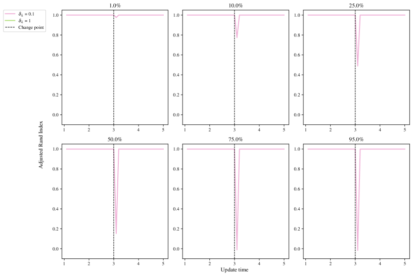
Refer to caption
(a) Mean ARI of the repetitions against update time for a varying proportion of group 1 nodes changing to group 2.
Refer to caption
(b) Mean over the repetitions of the proportion of nodes in group 1 with time. The results obtained when using no BFF (green line) and a BFF of 0.1 (pink line) are shown together on each panel. The true proportion of group 1 either side of the changepoint is plotted as black, horizontal lines..
Figure 9: Detection of group membership changes for a varying percentage of nodes swapping from group 1 to group 2 at t=3𝑡3t=3. The panel titles give the percentage of nodes that swap from group 1 to 2.

Figure 9(a) shows the inference procedure is stable across all values of P𝑃P, where the plots begin from B1subscript𝐵1B_{1} steps. The ARI is steady before and after the change except for the step immediately after the change. Figure 9(b) shows that the algorithm quickly converges to the true proportions, both with and without a BFF.

4.2 Number of groups recovery

We consider a fully connected network with two group membership changes: all nodes merging into group 1 at t=2.5𝑡2.5t=2.5, followed by the creation of a new group at t=3.5𝑡3.5t=3.5. Specifically, at t=3.5𝑡3.5t=3.5, P%percent𝑃P\% of the nodes in group 1 remain, while the remainder create group 2. We again consider P{1,10,25,50,75,95}𝑃11025507595P\in\{1,10,25,50,75,95\}, with λ0subscript𝜆0\lambda_{0} as the rate matrix, and ARI as our performance metric. We set LJS=0subscript𝐿𝐽𝑆0L_{JS}=0 here, which corresponds to taking the argmax of each τisubscript𝜏𝑖\tau_{i}.

Figure 11 shows that the inference correctly groups the nodes in all cases pre-merger and between the merger and creation, both with and without a BFF. Using a BFF, the algorithm is seen to maintain a high ARI after the creation of a new group, in all cases except when P=75𝑃75P=75. The application without the BFF also fails in this case, but additionally it fails for P=50𝑃50P=50, and is slower to converge to the new groups when P=25𝑃25P=25 and 10.

For cases where 50% of nodes or less remain in group 1, the algorithm converges to the correct proportions, but with label-switching. This is observed in Figure 11, where the rates are seen to swap in the 10% panel for the case of a BFF.
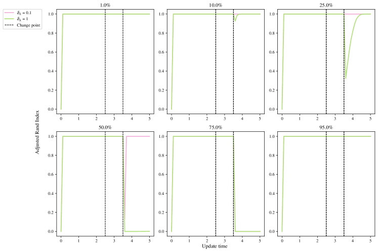
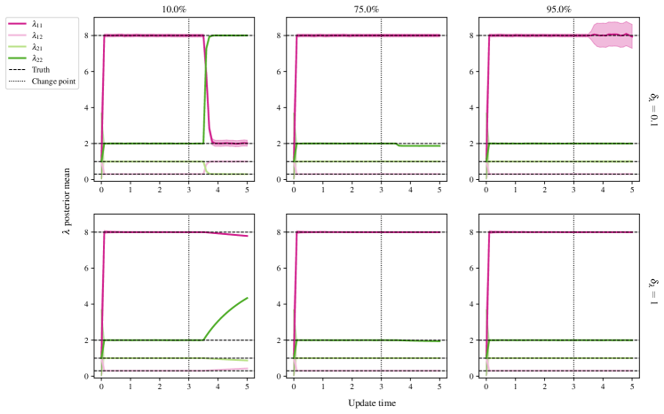
Refer to caption
Figure 10: Mean ARI against update time for the merger of group 2 into 1 at t=2.5𝑡2.5t=2.5, and the creation of group 2 at t=3.5𝑡3.5t=3.5, with the panel titles giving the percentage of nodes remaining in group 1 after t=3.5𝑡3.5t=3.5. The black, dashed vertical lines mark the changepoints. At t=2.5𝑡2.5t=2.5, all nodes in group 2 change to group 1, and at t=3.5𝑡3.5t=3.5, P%percent𝑃P\% of group 1 nodes change to group 2, P{1,10,25,50,75,95}𝑃11025507595P\in\{1,10,25,50,75,95\}.
Refer to caption
Figure 11: Posterior means and 95% confidence interval for components λ𝜆\lambda with update time. The black, dashed vertical lines mark the changepoints. At t=2.5𝑡2.5t=2.5, all nodes in group 2 change to group 1, and at t=3.5𝑡3.5t=3.5, P%percent𝑃P\% of group 1 nodes change to group 2, P{10,75,95}𝑃107595P\in\{10,75,95\}.

4.3 Detection of changes to the matrix of rates

On a fully connected network, we examine sequential changes to the rate matrix with decreasing time between the changes. The rate matrix maps as

λ=(210.38)λ=(510.38)λ′′=(310.38),formulae-sequence𝜆matrix210.38maps-toformulae-sequencesuperscript𝜆matrix510.38maps-tosuperscript𝜆′′matrix310.38\lambda=\begin{pmatrix}2&1\\ 0.3&8\end{pmatrix}\quad\mapsto\quad\lambda^{\prime}=\begin{pmatrix}5&1\\ 0.3&8\end{pmatrix}\quad\mapsto\quad\lambda^{\prime\prime}=\begin{pmatrix}3&1\\ 0.3&8\end{pmatrix},

with the first change at t=3𝑡3t=3 and the second at t=3+0.1M𝑡30.1𝑀t=3+0.1M. For each run, M𝑀M took a value in {1,2,3,4,5,10}1234510\{1,2,3,4,5,10\}. Here we do not reset the stream after a flagged change to the latent rates as we control their relative magnitude and wish to examine the performance of the algorithm with small latency between changes.

We evaluate the detection of latent changes using the proportion of changepoints correctly detected (CCD), and the proportion of detections that are not false (DNF), as in Bodenham and Adams (2017). Note that we aggregate across all group-to-group rates. Specifically, if there are C𝐶C changepoints, and we detect D𝐷D, T𝑇T of which are correct, analogous to recall and precision, the authors define:

  1. 1.

    CCD=T/CCCD𝑇𝐶\mathrm{CCD}=T/C, the proportion of changepoints correctly detected,

  2. 2.

    DNF=T/DDNF𝑇𝐷\mathrm{DNF}=T/D, the proportion of detections that are not false.

As noted by Bodenham and Adams (2017), CCD and DNF are preferred to their more intuitive counterparts (proportion of missed changepoints and proportion of false detections, respectively) as for the CCD and DNF, values closer to 1 indicate better performance than those closer to 0. Furthermore, these metrics are preferable over average run length metrics (ARL0ARL0\mathrm{ARL}0 and ARL1ARL1\mathrm{ARL}1) as we want to capture the number of changes detected and missed.

Suppose tnsubscriptsuperscript𝑡𝑛t^{\ast}_{n} and tn+1subscriptsuperscript𝑡𝑛1t^{\ast}_{n+1} are consecutive true changepoints for λkmsubscript𝜆𝑘𝑚\lambda_{km}, and let the most recently flagged changepoint by the algorithm for λkmsubscript𝜆𝑘𝑚\lambda_{km} be t<tnsubscriptsuperscript𝑡subscriptsuperscript𝑡𝑛t^{\prime}_{\ell}<t^{\ast}_{n}. If the next flag for λkmsubscript𝜆𝑘𝑚\lambda_{km} occurs at t+1>tn+1subscriptsuperscript𝑡1subscriptsuperscript𝑡𝑛1t^{\prime}_{\ell+1}>t^{\ast}_{n+1}, that is tnsubscriptsuperscript𝑡𝑛t^{\ast}_{n} is missed, then tm+1subscriptsuperscript𝑡𝑚1t^{\prime}_{m+1} is classified as a correct detection of tn+1subscriptsuperscript𝑡𝑛1t^{\ast}_{n+1}. This is common practice in the literature. This approach is adopted by Bodenham and Adams (2017), whereas other authors implement a softmax rule for classification (see, for example, Alanqary et al., 2021; Yamanishi and Takeuchi, 2002; Bodenham and Adams, 2017), adjusting for when multiple changes are flagged in the same window.
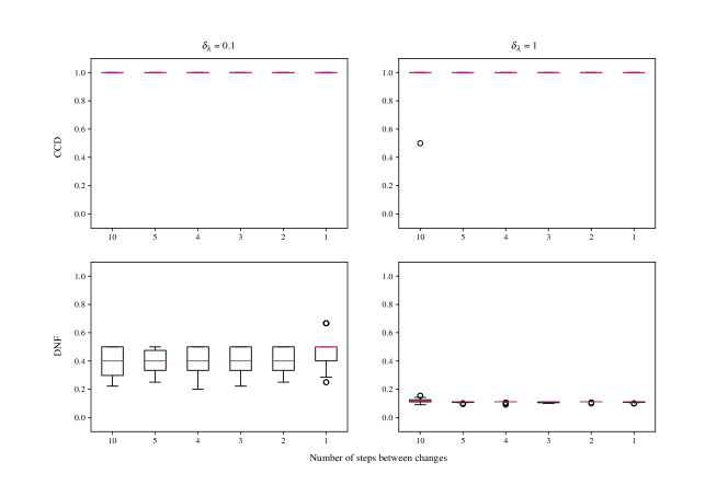
Refer to caption
Figure 12: Boxplots of CCD and DNF over 50 runs for no BFF and a BFF of δ=0.1𝛿0.1\delta=0.1. Each simulation has one change at t=3𝑡3t=3 and another a t=3+0.1M𝑡30.1𝑀t=3+0.1M, where M𝑀M is on the horizontal axis.

In Figure 12, we see the CCD and DNF for each run. The CCD is consistently high for both a BFF and no BFF. This demonstrates that the algorithm consistently flags true changes with and without a BFF. The role of the BFF is shown in the DNF, where we see BFF yielding higher values. Without a BFF, multiple changes are flagged that did not occur.

4.4 Effect of network sparsity

We examine the effect of decreasing network sparsity on changepoint detection. We simulate a network with K=1superscript𝐾1K^{\prime}=1 latent connection groups, letting ρ𝜌\rho, the group connection probability, vary over {0.01,0.025,0.05,0.1,0.25,0.5}0.010.0250.050.10.250.5\{0.01,0.025,0.05,0.1,0.25,0.5\}. For the point process groups, we retain the same ΠΠ\Pi as before, and again, we set λ=λ0𝜆subscript𝜆0\lambda=\lambda_{0}. We simulate on [0,25]025[0,25], with Δ=0.1Δ0.1\Delta=0.1, and at t=10𝑡10t=10, 25%percent2525\% of nodes from group 1 swap to group 2. The inference procedure is run on the simulated network twice, once where the network is assumed fully-connected, and a second time when the adjacency matrix is inferred. Both procedures are run with δ=0.1𝛿0.1\delta=0.1.

Figure 14 demonstrates the effect of incorrectly assuming that the graph is fully connected: the rates are significantly underestimated. On the other hand, when 𝑨𝑨\bm{A} is inferred, the posterior means are much closer to the true values, even in the case of 1%percent11\% density. Furthermore, in Figure 14 the mean ARI of the membership recovery is seen to be higher for the inferred adjacency matrix.
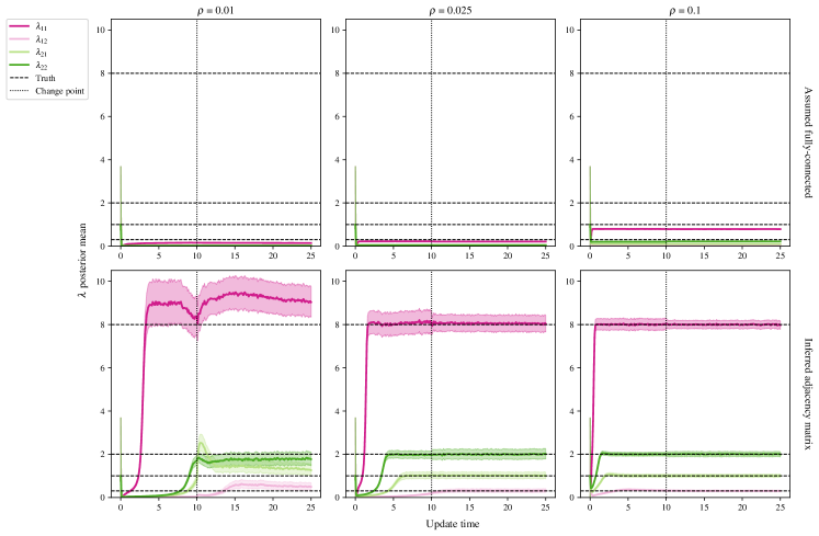
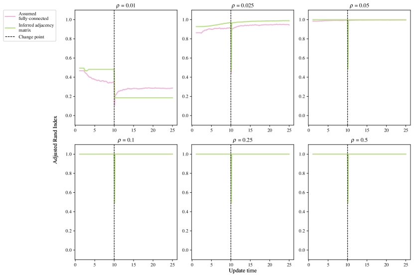
Refer to caption
Figure 13: Posterior means and 95% confidence interval for components λ𝜆\lambda with update time. The black, dashed vertical line marks the changepoint, at which 25%percent2525\% of nodes in group 1 swap to group 2.
Refer to caption
Figure 14: Mean ARI of the repetitions against update time. The black, dashed vertical line marks the changepoint, at which 25%percent2525\% of nodes in group 1 swap to group 2.

5 Application to the Santander Cycles bike-sharing network

The proposed online changepoint algorithms were tested on Transport for London (TfL) data from the London Santander Cycles bike-sharing network, which is publicly available online (https://cycling.data.tfl.gov.uk/, powered by TfL Open Data). Each datum corresponds to a bike hire, and contains the start and end times of the journey, the IDs of the source and destination stations, the journey duration, a bike ID number, and an unique identifier for the journey. Considering the start and end stations as source and destination nodes, and the timestamp of the end of the journey as an arrival time to the directed edge from source to destination, the data forms a network point process. In this study, the data is aggregated into weekly counts to smooth the intensities of the point processes and weekly periodicities. We select a subset of the data from 2nd January 2019 until 15th July 2020 as this window contains significant COVID-19 related national events that can be used to check the performance of our algorithm. In this time period, N=791𝑁791N=791 unique nodes are observed within T=80𝑇80T=80 weekly time windows, with updates every Δ=1Δ1\Delta=1 week time steps.

The online VB algorithm for the dynamic BHPP is run for the separate cases of an unknown graph structure, and an unknown number of groups. The number of groups in the case of an unknown adjacency matrix was set to match the number inferred by the implementation for an unknown number of groups, which was K=6𝐾6K=6. The adjacency matrix in the case of unknown K𝐾K was set to correspond to a fully connected graph: 𝑨=𝟏791×791𝑨subscript1791791\bm{A}=\bm{1}_{791\times 791}. We consider the task of detecting changes to the latent group structure of the bike sharing network. We run both algorithms with LJS=1.55subscript𝐿𝐽𝑆1.55L_{JS}=1.55, B1=25subscript𝐵125B_{1}=25, B2=10subscript𝐵210B_{2}=10, and κ=2𝜅2\kappa=2, so that changes can be detected only after B1+B2+κ=37subscript𝐵1subscript𝐵2𝜅37B_{1}+B_{2}+\kappa=37 weeks of observations. We initialise the hyperparameters as described in Section 4.
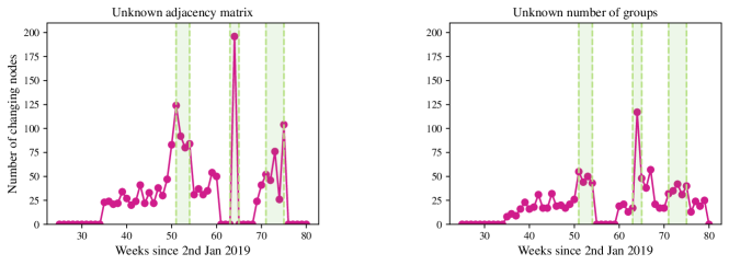
Refer to caption
Figure 15: The number of nodes that change memberships at each update point from initialisation. The green regions correspond to the Christmas and New Year period of 2019, the introduction of the first UK COVID-19 lockdown, and the phased easing of these restrictions, respectively.

Figure 15 shows that the algorithms flag multiple changes at each update, but that there are three regions where the number of flagged changes peaks. From left to right, these green regions correspond to the Christmas and New Year period of 2019, the introduction of the first UK COVID-19 lockdown on 19/03/2020, and the subsequent phased easing of restrictions from 01/06/2020. The algorithm reacts to these events, which are likely to cause changes to the network.
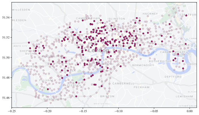
Refer to caption
Figure 16: Station locations with those stations that change group at the onset of the UK COVID-19 lockdown coloured dark red.

Figure 16 shows that the flagged changes corresponding to the onset of the lockdown are very concentrated around central London, which makes sense as “work from home” orders will have affected the use of these commuting bike stations. Additionally, stations around the Westfield Shopping Centre in Shepherd’s Bush and the Canary Wharf financial district are flagged, representing an expected change due to the government restrictions.

Furthermore, Figure 17 displays an example clustering from the dynamic BHPP model with unknown number of groups at update point 50. There is some spatial clustering to the nodes, but each cluster contains mainly nodes with similar activity patterns. For example, the dark and light blue clusters represent popular nodes in central London and the Canary Wharf financial district, which are mainly used by commuters into these areas. Similarly, the light and dark green clusters are nodes in West and East London (with the dark green cluster mostly covering West London, and the light green East London and the areas of Battersea and Wandsworth (south of the river Thames). The pink cluster is around the boundary between the blue and green regions. A notable exception is represented by the red cluster, representing the most popular stations within the network, mainly used for leisure around Hyde Park and the Queen Elizabeth Olympic Park in Stratford. In addition, the red cluster also contains two additional stations in Battersea Park and Ravenscourt Park (west of Hammersmith).
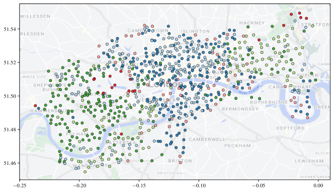
Refer to caption
Figure 17: Station locations coloured by assigned group at update step 50 of the dynamic BHPP with an unknown number of groups and 𝑨=𝟏791×791𝑨subscript1791791\bm{A}=\bm{1}_{791\times 791}.

6 Conclusion and discussion

We have presented a novel online Bayesian inference framework for detecting changes to the latent structure of a block-homogeneous Poisson process in which data arrives as batches in an event stream. Our methodology is scalable, and leverages a Bayesian forgetting factor framework to flag changes to the latent community structure and edge-process rates. The framework is extended to the cases where the adjacency matrix or the number of latent groups are unknown a priori. When tested on both real and simulated data, our methodology is seen to detect latent structure accurately and with minimal latency.

There are numerous ways in which this work could be extended. In particular, the frameworks for an unknown graph structure and unknown number of latent groups can readily be integrated to handle the case where neither is known a priori. It would also be of interest to incorporate seasonality into the model, perhaps within an online framework with longer memory.

A further challenge would be to adapt the framework to allow for nodes to enter or leave the network during observation. Similarly, the adjacency matrix is assumed static in our methodology, and so an extension would allow for this to be dynamic, although this would likely cause identifiability issues in the case where there are also changes to the latent rates.

Acknowledgements

Joshua Corneck acknowledges funding from the Engineering and Physical Sciences Research Council (EPSRC), grant number EP/S023151/1. Ed Cohen acknowledges funding from the EPSRC NeST Programme, grant number EP/X002195/1. Francesco Sanna Passino acknowledges funding from the EPSRC, grant number EP/Y002113/1.

Code

Python code to implement the methodologies proposed in this article and reproduce the results is available in the Github repository joshcorneck/dynamicBHPP.

References

  • Airoldi et al. (2013) Airoldi, E. M., Costa, T. B., and Chan, S. H. (2013) Stochastic blockmodel approximation of a graphon: Theory and consistent estimation. In Advances in Neural Information Processing Systems (eds. C. Burges, L. Bottou, M. Welling, Z. Ghahramani and K. Weinberger), vol. 26. Curran Associates, Inc.
  • Alanqary et al. (2021) Alanqary, A., Alomar, A. O., and Shah, D. (2021) Change point detection via multivariate singular spectrum analysis. In Advances in Neural Information Processing Systems (eds. A. Beygelzimer, Y. Dauphin, P. Liang and J. W. Vaughan).
  • Amini et al. (2013) Amini, A. A., Chen, A., Bickel, P. J., and Levina, E. (2013) Pseudo-likelihood methods for community detection in large sparse networks. The Annals of Statistics, 41, 2097–2122.
  • Bifet et al. (2018) Bifet, A., Gavaldà, R., Holmes, G., and Pfahringer, B. (2018) Machine Learning for Data Streams: with Practical Examples in MOA. Adaptive Computation and Machine Learning series. MIT Press.
  • Bishop (2006) Bishop, C. M. (2006) Pattern Recognition and Machine Learning (Information Science and Statistics). Berlin, Heidelberg: Springer-Verlag.
  • Blei and Jordan (2006) Blei, D. M. and Jordan, M. I. (2006) Variational inference for Dirichlet process mixtures. Bayesian Analysis, 1, 121–143.
  • Blei et al. (2017) Blei, D. M., Kucukelbir, A., and McAuliffe, J. D. (2017) Variational inference: A review for statisticians. Journal of the American Statistical Association, 112, 859–877.
  • Bodenham and Adams (2017) Bodenham, D. A. and Adams, N. M. (2017) Continuous monitoring for changepoints in data streams using adaptive estimation. Statistics and Computing, 27, 1257–1270.
  • Fang et al. (2024) Fang, G., Ward, O. G., and Zheng, T. (2024) Online estimation and community detection of network point processes for event streams. Statistics and Computing, 34.
  • Ferguson (1973) Ferguson, T. S. (1973) A Bayesian analysis of some nonparametric problems. The Annals of Statistics, 1, 209–230.
  • Gao et al. (2018) Gao, C., Ma, Z., Zhang, A. Y., and Zhou, H. H. (2018) Community detection in degree-corrected block models. The Annals of Statistics, 46, 2153–2185.
  • Hallgren et al. (2023) Hallgren, K. L., Heard, N. A., and Turcotte, M. J. M. (2023) Changepoint detection on a graph of time series. Bayesian Analysis, 1–28.
  • Haykin (2002) Haykin, S. (2002) Adaptive filter theory. Upper Saddle River, NJ: Prentice Hall, 4th edn.
  • Heard et al. (2010) Heard, N. A., Weston, D. J., Platanioti, K., and Hand, D. J. (2010) Bayesian anomaly detection methods for social networks. The Annals of Applied Statistics, 4, 645–662.
  • Holland et al. (1983) Holland, P. W., Laskey, K. B., and Leinhardt, S. (1983) Stochastic blockmodels: First steps. Social Networks, 5, 109–137.
  • Holme (2015) Holme, P. (2015) Modern temporal network theory: a colloquium. The European Physical Journal B, 88, 234.
  • Hubert and Arabie (1985) Hubert, L. J. and Arabie, P. (1985) Comparing partitions. Journal of Classification, 2, 193–218.
  • Jasra et al. (2005) Jasra, A., Holmes, C. C., and Stephens, D. A. (2005) Markov Chain Monte Carlo methods and the label switching problem in Bayesian mixture modeling. Statistical Science, 20, 50–67.
  • Karrer and Newman (2011) Karrer, B. and Newman, M. E. J. (2011) Stochastic blockmodels and community structure in networks. Physical Review E, 83, 016107.
  • Klimt and Yang (2004) Klimt, B. and Yang, Y. (2004) The Enron corpus: A new dataset for email classification research. In Machine Learning: ECML 2004 (eds. J.-F. Boulicaut, F. Esposito, F. Giannotti and D. Pedreschi), 217–226. Berlin, Heidelberg: Springer Berlin Heidelberg.
  • Lee and Wilkinson (2019) Lee, C. and Wilkinson, D. J. (2019) A review of stochastic block models and extensions for graph clustering. Applied Network Science, 4, 1–50.
  • Leys et al. (2013) Leys, C., Ley, C., Klein, O., Bernard, P., and Licata, L. (2013) Detecting outliers: Do not use standard deviation around the mean, use absolute deviation around the median. Journal of Experimental Social Psychology, 49, 764–766.
  • Lin (1991) Lin, J. (1991) Divergence measures based on the Shannon entropy. IEEE Transactions on Information Theory, 37, 145–151.
  • Mariadassou et al. (2010) Mariadassou, M., Robin, S., and Vacher, C. (2010) Uncovering latent structure in valued graphs: A variational approach. The Annals of Applied Statistics, 4.
  • Mariadassou and Tabouy (2020) Mariadassou, M. and Tabouy, T. (2020) Consistency and asymptotic normality of stochastic block models estimators from sampled data. The Electronic Journal of Statistics, 14, 3672–3704.
  • Matias and Miele (2017) Matias, C. and Miele, V. (2017) Statistical clustering of temporal networks through a dynamic stochastic block model. Journal of the Royal Statistical Society. Series B (Statistical Methodology), 79, 1119–1141.
  • Matias et al. (2018) Matias, C., Rebafka, T., and Villers, F. (2018) A semiparametric extension of the stochastic block model for longitudinal networks. Biometrika, 105, 665–680.
  • Paranjape et al. (2017) Paranjape, A., Benson, A. R., and Leskovec, J. (2017) Motifs in temporal networks. In Proceedings of the Tenth ACM International Conference on Web Search and Data Mining, WSDM ’17, 601–610. New York, NY, USA: Association for Computing Machinery.
  • Perry and Wolfe (2013) Perry, P. O. and Wolfe, P. J. (2013) Point process modelling for directed interaction networks. Journal of the Royal Statistical Society Series B: Statistical Methodology, 75, 821–849.
  • Pitman (2002) Pitman, J. (2002) Combinatorial stochastic processes (Technical Report 621). Department of Statistics. University of California at Berkeley, Berkeley, CA.
  • Ray and Szabó (2022) Ray, K. and Szabó, B. (2022) Variational Bayes for high-dimensional linear regression with sparse priors. Journal of the American Statistical Association, 117, 1270–1281.
  • Sanna Passino and Heard (2023) Sanna Passino, F. and Heard, N. A. (2023) Mutually exciting point process graphs for modeling dynamic networks. Journal of Computational and Graphical Statistics, 32, 116–130.
  • Sethuraman (1994) Sethuraman, J. (1994) A constructive definition of Dirichlet priors. Statistica Sinica, 639–650.
  • Shlomovich et al. (2022) Shlomovich, L., Cohen, E. A. K., and Adams, N. (2022) A parameter estimation method for multivariate binned Hawkes processes. Statistics and Computing, 32, 98.
  • van Dyk and Park (2008) van Dyk, D. A. and Park, T. (2008) Partially collapsed Gibbs samplers. Journal of the American Statistical Association, 103, 790–796.
  • Wang and Blei (2019) Wang, Y. and Blei, D. M. (2019) Frequentist consistency of variational Bayes. Journal of the American Statistical Association, 114, 1147–1161.
  • Xu and Hero (2014) Xu, K. and Hero, A. (2014) Dynamic stochastic blockmodels for time-evolving social networks. IEEE Journal of Selected Topics in Signal Processing, 8, 552–562.
  • Yamanishi and Takeuchi (2002) Yamanishi, K. and Takeuchi, J. (2002) A unifying framework for detecting outliers and change points from non-stationary time series data. In Proceedings of the Eighth ACM SIGKDD International Conference on Knowledge Discovery and Data Mining, KDD ’02, 676–681. New York, NY, USA: Association for Computing Machinery.
  • Yang et al. (2011) Yang, T., Chi, Y., Zhu, S., Gong, Y., and Jin, R. (2011) Detecting communities and their evolutions in dynamic social networks - a Bayesian approach. Machine Learning, 82, 157–189.
  • Zhang and Zhou (2020) Zhang, A. Y. and Zhou, H. H. (2020) Theoretical and computational guarantees of mean field variational inference for community detection. The Annals of Statistics, 48, 2575–2598.

Appendix A Derivation of CAVI updates

Here we derive the CAVI approximating distributions for each parameter at the r𝑟rth update. In deriving these expressions, we assume no ordering for the parameter updates, and will use a superscript of (r1)𝑟1(r-1) for all parameters but for the one whose expression is then being derived.

A.1 Approximation of q(zi)𝑞subscript𝑧𝑖q(z_{i})

Ignoring any terms that do not contain zisubscript𝑧𝑖z_{i}, we can derive the expectation as follows:

𝔼zisubscript𝔼subscript𝑧𝑖\displaystyle\mathbb{E}_{-z_{i}} {logp(x,z,λ,π)}=𝔼zi{logp(x|z,λ)+δzlogp(z|π)}+cst.𝑝𝑥𝑧𝜆𝜋subscript𝔼subscript𝑧𝑖𝑝conditional𝑥𝑧𝜆subscript𝛿𝑧𝑝conditional𝑧𝜋cst.\displaystyle\{\log p(x,z,\lambda,\pi)\}=\mathbb{E}_{-z_{i}}\left\{\log p(x|z,\lambda)+\delta_{z}\log p(z|\pi)\right\}+\text{cst.} (A.1)
=\displaystyle= 𝔼zi[j:(i,j)k,m𝒦z~ikz~jm(xij(Ir)log(λkm)Δλkm)+\displaystyle\ \mathbb{E}_{-z_{i}}\Bigg{[}\sum_{j:(i,j)\in\mathcal{E}}\sum_{k,m\in\mathcal{K}}\tilde{z}_{ik}\tilde{z}_{jm}\bigg{(}x_{ij}(I_{r})\log(\lambda_{km})-\Delta\lambda_{km}\bigg{)}+ (A.2)
j:(j,i)k,m𝒦z~jkz~im(xji(Ir)log(λkm)Δλkm)limit-fromsubscript:superscript𝑗superscript𝑗𝑖subscript𝑘𝑚𝒦subscript~𝑧superscript𝑗𝑘subscript~𝑧𝑖𝑚subscript𝑥superscript𝑗𝑖subscript𝐼𝑟subscript𝜆𝑘𝑚Δsubscript𝜆𝑘𝑚\displaystyle\qquad\qquad\sum_{j^{\prime}:(j^{\prime},i)\in\mathcal{E}}\sum_{k,m\in\mathcal{K}}\tilde{z}_{j^{\prime}k}\tilde{z}_{im}\bigg{(}x_{j^{\prime}i}(I_{r})\log(\lambda_{km})-\Delta\lambda_{km}\bigg{)}- (A.3)
k𝒦z~ik(xii(t)log(λkk)Δλkk)+δzk𝒦z~iklogπk]+cst.\displaystyle\qquad\qquad\sum_{k\in\mathcal{K}}\tilde{z}_{ik}\bigg{(}x_{ii}(t)\log(\lambda_{kk})-\Delta\lambda_{kk}\bigg{)}+\delta_{z}\sum_{k\in\mathcal{K}}\tilde{z}_{ik}\log\pi_{k}\Bigg{]}+\text{cst.} (A.4)
=\displaystyle= k𝒦z~ik[δz𝔼π{logπk}+xii(t)𝔼λkk{log(λkk)}Δ𝔼λkk{λkk}+\displaystyle\sum_{k\in\mathcal{K}}\tilde{z}_{ik}\Bigg{[}\delta_{z}\mathbb{E}_{\pi}\{\log\pi_{k}\}+x_{ii}(t)\mathbb{E}_{\lambda_{kk}}\{\log(\lambda_{kk})\}-\Delta\mathbb{E}_{\lambda_{kk}}\{\lambda_{kk}\}+ (A.5)
m𝒦{j:(i,j)𝔼zj{z~jm}(xij(Ir)𝔼λkm{log(λkm)}Δ𝔼λkm{λkm})(1𝕀{k}(m)𝕀{i}(j))+\displaystyle\sum_{m\in\mathcal{K}}\Bigg{\{}\sum_{j:(i,j)\in\mathcal{E}}\mathbb{E}_{z_{j}}\{\tilde{z}_{jm}\}\bigg{(}x_{ij}(I_{r})\mathbb{E}_{\lambda_{km}}\{\log(\lambda_{km})\}-\Delta\mathbb{E}_{\lambda_{km}}\{\lambda_{km}\}\bigg{)}\bigg{(}1-\mathbb{I}_{\{k\}}(m)\mathbb{I}_{\{i\}}(j)\bigg{)}+ (A.6)
j:(j,i)𝔼z~j{z~jm}(xji(Ir)𝔼λmk{log(λmk)}Δ𝔼λmk{λmk})(1𝕀{k}(m)𝕀{i}(j))}]+cst.\displaystyle\sum_{j^{\prime}:(j^{\prime},i)\in\mathcal{E}}\mathbb{E}_{\tilde{z}_{j^{\prime}}}\{\tilde{z}_{j^{\prime}m}\}\bigg{(}x_{j^{\prime}i}(I_{r})\mathbb{E}_{\lambda_{mk}}\{\log(\lambda_{mk})\}-\Delta\mathbb{E}_{\lambda_{mk}}\{\lambda_{mk}\}\bigg{)}\bigg{(}1-\mathbb{I}_{\{k\}}(m)\mathbb{I}_{\{i\}}(j^{\prime})\bigg{)}\Bigg{\}}\Bigg{]}+\text{cst.} (A.7)

Taking the exponential, it follows that the optimal choice of q^(zi)^𝑞subscript𝑧𝑖\hat{q}(z_{i}) under a CAVI approximation is q^(r)(zi)=Categorical(zi;τi(r))superscript^𝑞𝑟subscript𝑧𝑖Categoricalsubscript𝑧𝑖superscriptsubscript𝜏𝑖𝑟\hat{q}^{(r)}(z_{i})=\mathrm{Categorical}\left(z_{i};\tau_{i}^{(r)}\right), where

τik(r)superscriptsubscript𝜏𝑖𝑘𝑟\displaystyle\tau_{ik}^{(r)} exp{δz[ψ(γk(r1))ψ(γ(r1))]+xii(t)(ψ(αkk(r1))log(βkk(r1)))Δαkk(r1)βkk(r1)+\displaystyle\propto\exp\Bigg{\{}\delta_{z}\Bigg{[}\psi\left(\gamma^{(r-1)}_{k}\right)-\psi\left(\sum_{\ell}\gamma^{(r-1)}_{\ell}\right)\Bigg{]}+x_{ii}(t)\bigg{(}\psi\left(\alpha^{(r-1)}_{kk}\right)-\log\left(\beta^{(r-1)}_{kk}\right)\bigg{)}-\Delta\frac{\alpha^{(r-1)}_{kk}}{\beta^{(r-1)}_{kk}}+ (A.8)
m𝒦[j:(i,j)τjm(r1)(xij(Ir)(ψ(αkm(r1))log(βkm(r1)))Δαkm(r1)βkm(r1))(1𝕀{k}(m)𝕀{i}(j))+\displaystyle\qquad\sum_{m\in\mathcal{K}}\Bigg{[}\sum_{j:(i,j)\in\mathcal{E}}\tau^{(r-1)}_{jm}\bigg{(}x_{ij}(I_{r})\left(\psi\left(\alpha^{(r-1)}_{km}\right)-\log\left(\beta^{(r-1)}_{km}\right)\right)-\Delta\frac{\alpha^{(r-1)}_{km}}{\beta^{(r-1)}_{km}}\bigg{)}\bigg{(}1-\mathbb{I}_{\{k\}}(m)\mathbb{I}_{\{i\}}(j)\bigg{)}\ + (A.9)
j:(j,i)τjm(r1)(xji(Ir)(ψ(αmk(r1))log(βmk(r1)))Δαmk(r1)βmk(r1))(1𝕀{k}(m)𝕀{i}(j))]},\displaystyle\qquad\sum_{j^{\prime}:(j^{\prime},i)\in\mathcal{E}}\tau_{j^{\prime}m}^{(r-1)}\bigg{(}x_{j^{\prime}i}(I_{r})\left(\psi\left(\alpha^{(r-1)}_{mk}\right)-\log\left(\beta^{(r-1)}_{mk}\right)\right)-\Delta\frac{\alpha^{(r-1)}_{mk}}{\beta^{(r-1)}_{mk}}\bigg{)}\bigg{(}1-\mathbb{I}_{\{k\}}(m)\mathbb{I}_{\{i\}}(j^{\prime})\bigg{)}\Bigg{]}\Bigg{\}}, (A.10)

for i𝒱𝑖𝒱i\in\mathcal{V} and k𝒦𝑘𝒦k\in\mathcal{K}.

A.2 Approximation of q(π)𝑞𝜋q(\pi)

Ignoring any terms that do not contain π𝜋\pi, we compute the expectation as:

𝔼πsubscript𝔼𝜋\displaystyle\mathbb{E}_{-\pi} {logp(x,z,λ,π)}=𝔼π{δzlogp(z|π)+δπlogp(π)}+cst.𝑝𝑥𝑧𝜆𝜋subscript𝔼𝜋subscript𝛿𝑧𝑝conditional𝑧𝜋subscript𝛿𝜋𝑝𝜋cst.\displaystyle\left\{\log p(x,z,\lambda,\pi)\right\}=\mathbb{E}_{-\pi}\left\{\delta_{z}\log p(z|\pi)+\delta_{\pi}\log p(\pi)\right\}+\text{cst.} (A.11)
=k𝒦logπk[i𝒱δz𝔼zi{z~ik}+δπ(γk(r1)1)]+cst.absentsubscript𝑘𝒦subscript𝜋𝑘delimited-[]subscript𝑖𝒱subscript𝛿𝑧subscript𝔼subscript𝑧𝑖subscript~𝑧𝑖𝑘subscript𝛿𝜋superscriptsubscript𝛾𝑘𝑟11cst.\displaystyle=\sum_{k\in\mathcal{K}}\log\pi_{k}\left[\sum_{i\in\mathcal{V}}\delta_{z}\mathbb{E}_{z_{i}}\{\tilde{z}_{ik}\}+\delta_{\pi}\left(\gamma_{k}^{(r-1)}-1\right)\right]+\text{cst.} (A.12)

Using the distributions derived for q^(r1)(zi)superscript^𝑞𝑟1subscript𝑧𝑖\hat{q}^{(r-1)}(z_{i}), we see that the optional CAVI approximation is to take q^(r)(π)=Dirichlet(π;γ(r))superscript^𝑞𝑟𝜋Dirichlet𝜋superscript𝛾𝑟\hat{q}^{(r)}(\pi)=\mathrm{Dirichlet}\left(\pi;\gamma^{(r)}\right), where

γk(r)=δπ(γk(r1)1)+δzi𝒱τik(r1)+1,superscriptsubscript𝛾𝑘𝑟subscript𝛿𝜋superscriptsubscript𝛾𝑘𝑟11subscript𝛿𝑧subscript𝑖𝒱subscriptsuperscript𝜏𝑟1𝑖𝑘1\gamma_{k}^{(r)}=\delta_{\pi}\left(\gamma_{k}^{(r-1)}-1\right)+\delta_{z}\sum_{i\in\mathcal{V}}\tau^{(r-1)}_{ik}+1, (A.13)

for k𝒦𝑘𝒦k\in\mathcal{K}.

A.3 Approximation of q(λkm)𝑞subscript𝜆𝑘𝑚q(\lambda_{km})

Ignoring any terms that do not contain λkmsubscript𝜆𝑘𝑚\lambda_{km}, we derive the expectation as follows:

𝔼λkmsubscript𝔼subscript𝜆𝑘𝑚\displaystyle\mathbb{E}_{-\lambda_{km}} {logp(x,z,λ,π)}=𝔼λkm{logp(x|z,λ)+δλlogp(λ)}+cst.𝑝𝑥𝑧𝜆𝜋subscript𝔼subscript𝜆𝑘𝑚𝑝conditional𝑥𝑧𝜆subscript𝛿𝜆𝑝𝜆cst.\displaystyle\left\{\log p(x,z,\lambda,\pi)\right\}=\mathbb{E}_{-\lambda_{km}}\left\{\log p(x|z,\lambda)+\delta_{\lambda}\log p(\lambda)\right\}+\text{cst.} (A.14)
=(i,j)k,m𝒦[𝔼zi{z~ik}𝔼zj{z~jm}(xijlogλkmλkmΔ)]+absentlimit-fromsubscript𝑖𝑗subscript𝑘𝑚𝒦delimited-[]subscript𝔼subscript𝑧𝑖subscript~𝑧𝑖𝑘subscript𝔼subscript𝑧𝑗subscript~𝑧𝑗𝑚subscript𝑥𝑖𝑗subscript𝜆𝑘𝑚subscript𝜆𝑘𝑚Δ\displaystyle=\ \sum_{(i,j)\in\mathcal{E}}\sum_{k,m\in\mathcal{K}}\bigg{[}\mathbb{E}_{z_{i}}\{\tilde{z}_{ik}\}\mathbb{E}_{z_{j}}\{\tilde{z}_{jm}\}(x_{ij}\log\lambda_{km}-\lambda_{km}\Delta)\bigg{]}+ (A.15)
δλk,m𝒦[(αkm(r1)1)logλkmβkm(r1)λkm]+cst.subscript𝛿𝜆subscript𝑘𝑚𝒦delimited-[]subscriptsuperscript𝛼𝑟1𝑘𝑚1subscript𝜆𝑘𝑚subscriptsuperscript𝛽𝑟1𝑘𝑚subscript𝜆𝑘𝑚cst.\displaystyle\quad\delta_{\lambda}\sum_{k,m\in\mathcal{K}}\left[\left(\alpha^{(r-1)}_{km}-1\right)\log\lambda_{km}-\beta^{(r-1)}_{km}\lambda_{km}\right]+\text{cst.} (A.16)
=k,m𝒦{(δλ(αkm(r1)1)+(i,j)𝔼zi{z~ik}𝔼zj{z~ik}xij(Ir))logλkm\displaystyle=\sum_{k,m\in\mathcal{K}}\bigg{\{}\bigg{(}\delta_{\lambda}\left(\alpha^{(r-1)}_{km}-1\right)+\sum_{(i,j)\in\mathcal{E}}\mathbb{E}_{z_{i}}\{\tilde{z}_{ik}\}\mathbb{E}_{z_{j}}\{\tilde{z}_{ik}\}x_{ij}(I_{r})\bigg{)}\log\lambda_{km}\ - (A.17)
(δλβkm(r1)+Δ(i,j)𝔼zi{z~ik}𝔼zj{z~ik})λkm}+cst.\displaystyle\quad\left(\delta_{\lambda}\beta^{(r-1)}_{km}+\Delta\sum_{(i,j)\in\mathcal{E}}\mathbb{E}_{z_{i}}\{\tilde{z}_{ik}\}\mathbb{E}_{z_{j}}\{\tilde{z}_{ik}\}\right)\lambda_{km}\bigg{\}}+\text{cst.} (A.18)

Using the distributions derived for q^(r1)(zi)superscript^𝑞𝑟1subscript𝑧𝑖\hat{q}^{(r-1)}(z_{i}), it follows that the optimal CAVI approximation is to take q^(r)(λkm)=Gamma(λkm;αkm(r),βkm(r))superscript^𝑞𝑟subscript𝜆𝑘𝑚Gammasubscript𝜆𝑘𝑚subscriptsuperscript𝛼𝑟𝑘𝑚subscriptsuperscript𝛽𝑟𝑘𝑚\hat{q}^{(r)}\left(\lambda_{km}\right)=\mathrm{Gamma}\left(\lambda_{km};\alpha^{(r)}_{km},\beta^{(r)}_{km}\right), where

αkm(r)subscriptsuperscript𝛼𝑟𝑘𝑚\displaystyle\alpha^{(r)}_{km} =δλ(αkm(r1)1)+(i,j)τik(r1)τjm(r1)xij(Ir)+1,absentsubscript𝛿𝜆subscriptsuperscript𝛼𝑟1𝑘𝑚1subscript𝑖𝑗subscriptsuperscript𝜏𝑟1𝑖𝑘subscriptsuperscript𝜏𝑟1𝑗𝑚subscript𝑥𝑖𝑗subscript𝐼𝑟1\displaystyle=\delta_{\lambda}\left(\alpha^{(r-1)}_{km}-1\right)+\sum_{(i,j)\in\mathcal{E}}\tau^{(r-1)}_{ik}\tau^{(r-1)}_{jm}x_{ij}(I_{r})+1, (A.19)
βkm(r)subscriptsuperscript𝛽𝑟𝑘𝑚\displaystyle\beta^{(r)}_{km} =δλβkm(r1)+Δ(i,j)τik(r1)τjm(r1),absentsubscript𝛿𝜆subscriptsuperscript𝛽𝑟1𝑘𝑚Δsubscript𝑖𝑗subscriptsuperscript𝜏𝑟1𝑖𝑘subscriptsuperscript𝜏𝑟1𝑗𝑚\displaystyle=\delta_{\lambda}\beta^{(r-1)}_{km}+\Delta\sum_{(i,j)\in\mathcal{E}}\tau^{(r-1)}_{ik}\tau^{(r-1)}_{jm}, (A.20)

for k,m𝒦𝑘𝑚𝒦k,m\in\mathcal{K}.

Appendix B Derivation of CAVI updates for an unknown adjacency matrix

Here we derive the CAVI approximating distributions for each parameter at the r𝑟rth update. In deriving these expressions, we assume no ordering for the parameter updates, and will use a superscript of (r1)𝑟1(r-1) for all parameters but for the one whose expression is then being derived.

B.1 Approximation of q(zi)𝑞subscript𝑧𝑖q(z_{i})

Ignoring any terms that do not contain zisubscript𝑧𝑖z_{i}, we derive the expectation as:

𝔼zisubscript𝔼subscript𝑧𝑖\displaystyle\mathbb{E}_{-z_{i}} {logp(x,z,a,λ,π)}=𝔼zi{logp(x|z,a,λ)+δzlogp(z|π)}+cst.𝑝𝑥𝑧𝑎𝜆𝜋subscript𝔼subscript𝑧𝑖𝑝conditional𝑥𝑧𝑎𝜆subscript𝛿𝑧𝑝conditional𝑧𝜋cst.\displaystyle\left\{\log p(x,z,a,\lambda,\pi)\right\}=\mathbb{E}_{-z_{i}}\left\{\log p(x|z,a,\lambda)+\delta_{z}\log p(z|\pi)\right\}+\text{cst.} (B.1)
=𝔼zi{j𝒱k,m𝒦z~ikz~jm[aij(xij(Ir)logλkmΔλkm)]+\displaystyle=\mathbb{E}_{-z_{i}}\Bigg{\{}\sum_{j\in\mathcal{V}}\sum_{k,m\in\mathcal{K}}\tilde{z}_{ik}\tilde{z}_{jm}\bigg{[}a_{ij}\left(x_{ij}(I_{r})\log\lambda_{km}-\Delta\lambda_{km}\right)\bigg{]}+ (B.2)
j𝒱k,m𝒦z~jkz~im[aji(xji(Ir)logλkmΔλkm)]limit-fromsubscriptsuperscript𝑗𝒱subscript𝑘𝑚𝒦subscript~𝑧superscript𝑗𝑘subscript~𝑧𝑖𝑚delimited-[]subscript𝑎superscript𝑗𝑖subscript𝑥superscript𝑗𝑖subscript𝐼𝑟subscript𝜆𝑘𝑚Δsubscript𝜆𝑘𝑚\displaystyle\qquad\qquad\sum_{j^{\prime}\in\mathcal{V}}\sum_{k,m\in\mathcal{K}}\tilde{z}_{j^{\prime}k}\tilde{z}_{im}\bigg{[}a_{j^{\prime}i}\left(x_{j^{\prime}i}(I_{r})\log\lambda_{km}-\Delta\lambda_{km}\right)\bigg{]}- (B.3)
k𝒦z~ik[aii(xii(Ir)logλkkΔλkk)]+δzk𝒦z~iklogπk}+cst.\displaystyle\qquad\qquad\sum_{k\in\mathcal{K}}\tilde{z}_{ik}\bigg{[}a_{ii}\left(x_{ii}(I_{r})\log\lambda_{kk}-\Delta\lambda_{kk}\right)\bigg{]}+\delta_{z}\sum_{k\in\mathcal{K}}\tilde{z}_{ik}\log\pi_{k}\Bigg{\}}+\text{cst.} (B.4)
=𝔼zi{j𝒱k,m𝒦z~ikz~jm[aij(xij(Ir)logλkmΔλkm)+aji(xji(Ir)logλmkΔλmk)]\displaystyle=\mathbb{E}_{-z_{i}}\Bigg{\{}\sum_{j\in\mathcal{V}}\sum_{k,m\in\mathcal{K}}\tilde{z}_{ik}\tilde{z}_{jm}\bigg{[}a_{ij}\left(x_{ij}(I_{r})\log\lambda_{km}-\Delta\lambda_{km}\right)+a_{ji}\left(x_{ji}(I_{r})\log\lambda_{mk}-\Delta\lambda_{mk}\right)\bigg{]}- (B.5)
k𝒦z~ik[aii(xii(Ir)logλkkΔλkk)]+δzk𝒦z~iklogπk}+cst.\displaystyle\qquad\qquad\sum_{k\in\mathcal{K}}\tilde{z}_{ik}\bigg{[}a_{ii}\left(x_{ii}(I_{r})\log\lambda_{kk}-\Delta\lambda_{kk}\right)\bigg{]}+\delta_{z}\sum_{k\in\mathcal{K}}\tilde{z}_{ik}\log\pi_{k}\Bigg{\}}+\text{cst.} (B.6)
=k𝒦z~ik{j𝒱m𝒦z~jm[xij(Ir)𝔼aij{aij}𝔼λkm{logλkm}+xji(Ir)𝔼aji{aji}𝔼λmk{logλmk}\displaystyle=\sum_{k\in\mathcal{K}}\tilde{z}_{ik}\Bigg{\{}\sum_{j\in\mathcal{V}}\sum_{m\in\mathcal{K}}\tilde{z}_{jm}\bigg{[}x_{ij}(I_{r})\mathbb{E}_{a_{ij}}\{a_{ij}\}\mathbb{E}_{\lambda_{km}}\{\log\lambda_{km}\}+x_{ji}(I_{r})\mathbb{E}_{a_{ji}}\{a_{ji}\}\mathbb{E}_{\lambda_{mk}}\{\log\lambda_{mk}\}\ - (B.7)
Δ(𝔼aij{aij}𝔼λkm{λkm}+𝔼aji{aji}𝔼λmk{λmk})](1𝕀{k}(m)𝕀{i}(j))+\displaystyle\qquad\qquad\Delta\bigg{(}\mathbb{E}_{a_{ij}}\{a_{ij}\}\mathbb{E}_{\lambda_{km}}\{\lambda_{km}\}+\mathbb{E}_{a_{ji}}\{a_{ji}\}\mathbb{E}_{\lambda_{mk}}\{\lambda_{mk}\}\bigg{)}\bigg{]}\bigg{(}1-\mathbb{I}_{\{k\}}(m)\mathbb{I}_{\{i\}}(j)\bigg{)}+ (B.8)
𝔼aii{aii}(xii(Ir)𝔼λkk{logλkk}Δ𝔼λkk{λkk})+δz𝔼πk{logπk}}+cst.\displaystyle\qquad\qquad\mathbb{E}_{a_{ii}}\{a_{ii}\}\bigg{(}x_{ii}(I_{r})\mathbb{E}_{\lambda_{kk}}\{\log\lambda_{kk}\}-\Delta\mathbb{E}_{\lambda_{kk}}\{\lambda_{kk}\}\bigg{)}+\delta_{z}\mathbb{E}_{\pi_{k}}\left\{\log\pi_{k}\right\}\Bigg{\}}+\text{cst.} (B.9)

Taking the exponential, and using the distributions derived for q^(r1)(λkm)superscript^𝑞𝑟1subscript𝜆𝑘𝑚\hat{q}^{(r-1)}(\lambda_{km}) and the assumed form for q^(r1)(aij)superscript^𝑞𝑟1subscript𝑎𝑖𝑗\hat{q}^{(r-1)}(a_{ij}), it follows that the optimal CAVI approximation is to take q^(r)(zi)=Categorical(zi;τi(r))superscript^𝑞𝑟subscript𝑧𝑖Categoricalsubscript𝑧𝑖subscriptsuperscript𝜏𝑟𝑖\hat{q}^{(r)}(z_{i})=\mathrm{Categorical}\left(z_{i};\tau^{(r)}_{i}\right), where

τik(r)subscriptsuperscript𝜏𝑟𝑖𝑘\displaystyle\tau^{(r)}_{ik} exp{j𝒱m𝒦τjm(r1)[σij(r1)xij(Ir)(ψ(αkm(r1))log(βkm(r1)))+\displaystyle\propto\exp\Bigg{\{}\sum_{j\in\mathcal{V}}\sum_{m\in\mathcal{K}}\tau^{(r-1)}_{jm}\bigg{[}\sigma^{(r-1)}_{ij}x_{ij}(I_{r})\bigg{(}\psi\left(\alpha^{(r-1)}_{km}\right)-\log\left(\beta^{(r-1)}_{km}\right)\bigg{)}\ + (B.10)
σji(r1)xji(Ir)(ψ(αmk(r1))log(βmk(r1)))Δ(σij(r1)αkm(r1)βkm(r1)+σji(r1)αmk(r1)βmk(r1))]×\displaystyle\quad\sigma^{(r-1)}_{ji}x_{ji}(I_{r})\bigg{(}\psi\left(\alpha^{(r-1)}_{mk}\right)-\log\left(\beta^{(r-1)}_{mk}\right)\bigg{)}-\Delta\bigg{(}\sigma^{(r-1)}_{ij}\frac{\alpha^{(r-1)}_{km}}{\beta^{(r-1)}_{km}}+\sigma^{(r-1)}_{ji}\frac{\alpha^{(r-1)}_{mk}}{\beta^{(r-1)}_{mk}}\bigg{)}\bigg{]}\ \times (B.11)
(1𝕀{k}(m)𝕀{i}(j))+σii(r1)(xii(Ir)(ψ(αkk(r1))log(βkk(r1)))Δαkk(r1)βkk(r1))+1subscript𝕀𝑘𝑚subscript𝕀𝑖𝑗limit-fromsubscriptsuperscript𝜎𝑟1𝑖𝑖subscript𝑥𝑖𝑖subscript𝐼𝑟𝜓subscriptsuperscript𝛼𝑟1𝑘𝑘subscriptsuperscript𝛽𝑟1𝑘𝑘Δsubscriptsuperscript𝛼𝑟1𝑘𝑘subscriptsuperscript𝛽𝑟1𝑘𝑘\displaystyle\quad\bigg{(}1-\mathbb{I}_{\{k\}}(m)\mathbb{I}_{\{i\}}(j)\bigg{)}+\sigma^{(r-1)}_{ii}\bigg{(}x_{ii}(I_{r})\bigg{(}\psi\left(\alpha^{(r-1)}_{kk}\right)-\log\left(\beta^{(r-1)}_{kk}\right)\bigg{)}-\Delta\frac{\alpha^{(r-1)}_{kk}}{\beta^{(r-1)}_{kk}}\bigg{)}\ + (B.12)
δz[ψ(γk(r1))ψ(γ(r1))]},\displaystyle\quad\delta_{z}\Bigg{[}\psi\left(\gamma^{(r-1)}_{k}\right)-\psi\left(\sum_{\ell}\gamma^{(r-1)}_{\ell}\right)\Bigg{]}\Bigg{\}}, (B.13)

for i𝒱𝑖𝒱i\in\mathcal{V} and k𝒦𝑘𝒦k\in\mathcal{K}.

B.2 Approximation of q(λkm)𝑞subscript𝜆𝑘𝑚q(\lambda_{km})

Ignoring any terms that do not contain λkmsubscript𝜆𝑘𝑚\lambda_{km}, we can derive the expectation as follows:

𝔼λkmsubscript𝔼subscript𝜆𝑘𝑚\displaystyle\mathbb{E}_{-\lambda_{km}} {logp(x,z,z,a,λ,ρ,π,μ)}=𝔼λkm{logp(x|z,a,λ)+δλlogp(λ)}+cst.𝑝𝑥𝑧superscript𝑧𝑎𝜆𝜌𝜋𝜇subscript𝔼subscript𝜆𝑘𝑚𝑝conditional𝑥𝑧𝑎𝜆subscript𝛿𝜆𝑝𝜆cst.\displaystyle\{\log p(x,z,z^{\prime},a,\lambda,\rho,\pi,\mu)\}=\mathbb{E}_{-\lambda_{km}}\bigg{\{}\log p(x|z,a,\lambda)+\delta_{\lambda}\log p(\lambda)\bigg{\}}+\text{cst.} (B.14)
=(i,j)𝔼zi{z~ik}𝔼zj{z~jm}𝔼aij{aij}(xij(Ir)logλkmΔλkm)+absentlimit-fromsubscript𝑖𝑗subscript𝔼subscript𝑧𝑖subscript~𝑧𝑖𝑘subscript𝔼subscript𝑧𝑗subscript~𝑧𝑗𝑚subscript𝔼subscript𝑎𝑖𝑗subscript𝑎𝑖𝑗subscript𝑥𝑖𝑗subscript𝐼𝑟subscript𝜆𝑘𝑚Δsubscript𝜆𝑘𝑚\displaystyle=\sum_{(i,j)\in\mathcal{R}}\mathbb{E}_{z_{i}}\{\tilde{z}_{ik}\}\mathbb{E}_{z_{j}}\{\tilde{z}_{jm}\}\mathbb{E}_{a_{ij}}\{a_{ij}\}\bigg{(}x_{ij}(I_{r})\log\lambda_{km}-\Delta\lambda_{km}\bigg{)}+ (B.15)
δλ((αkm(r1)1)logλkmβkm(r1)λkm)+cst.subscript𝛿𝜆superscriptsubscript𝛼𝑘𝑚𝑟11subscript𝜆𝑘𝑚superscriptsubscript𝛽𝑘𝑚𝑟1subscript𝜆𝑘𝑚cst.\displaystyle\quad\delta_{\lambda}\bigg{(}\bigg{(}\alpha_{km}^{(r-1)}-1\bigg{)}\log\lambda_{km}-\beta_{km}^{(r-1)}\lambda_{km}\bigg{)}+\text{cst.} (B.16)
=((i,j)𝔼zi{z~ik}𝔼zi{z~jm}𝔼+aij{aij}xij(Ir)+δλ(αkm(r1)1))logλkmabsentlimit-fromsubscript𝑖𝑗subscript𝔼subscript𝑧𝑖subscript~𝑧𝑖𝑘subscript𝔼subscript𝑧𝑖subscript~𝑧𝑗𝑚𝔼subscript𝑎𝑖𝑗subscript𝑎𝑖𝑗subscript𝑥𝑖𝑗subscript𝐼𝑟subscript𝛿𝜆superscriptsubscript𝛼𝑘𝑚𝑟11subscript𝜆𝑘𝑚\displaystyle=\bigg{(}\sum_{(i,j)\in\mathcal{R}}\mathbb{E}_{z_{i}}\{\tilde{z}_{ik}\}\mathbb{E}_{z_{i}}\{\tilde{z}_{jm}\}\mathbb{E}+{a_{ij}}\{a_{ij}\}x_{ij}(I_{r})+\delta_{\lambda}\bigg{(}\alpha_{km}^{(r-1)}-1\bigg{)}\bigg{)}\log\lambda_{km}\ - (B.17)
(Δ(i,j)𝔼zi{z~ik}𝔼zj{z~jm}𝔼aij{aij}+δλβkm(r1))λkm+cst.Δsubscript𝑖𝑗subscript𝔼subscript𝑧𝑖subscript~𝑧𝑖𝑘subscript𝔼subscript𝑧𝑗subscript~𝑧𝑗𝑚subscript𝔼subscript𝑎𝑖𝑗subscript𝑎𝑖𝑗subscript𝛿𝜆superscriptsubscript𝛽𝑘𝑚𝑟1subscript𝜆𝑘𝑚cst.\displaystyle\quad\bigg{(}\Delta\sum_{(i,j)\in\mathcal{R}}\mathbb{E}_{z_{i}}\{\tilde{z}_{ik}\}\mathbb{E}_{z_{j}}\{\tilde{z}_{jm}\}\mathbb{E}_{a_{ij}}\{a_{ij}\}+\delta_{\lambda}\beta_{km}^{(r-1)}\bigg{)}\lambda_{km}+\text{cst.} (B.18)

Using the distributions derived for q^(r1)(zi)superscript^𝑞𝑟1subscript𝑧𝑖\hat{q}^{(r-1)}(z_{i}) and assumed form for q^(r1)(aij)superscript^𝑞𝑟1subscript𝑎𝑖𝑗\hat{q}^{(r-1)}(a_{ij}), we see that the optimal CAVI approximating distribution is q^(r)(λkm)=Gamma(λkm;αkm(r),βkm(r))superscript^𝑞𝑟subscript𝜆𝑘𝑚Gammasubscript𝜆𝑘𝑚superscriptsubscript𝛼𝑘𝑚𝑟superscriptsubscript𝛽𝑘𝑚𝑟\hat{q}^{(r)}(\lambda_{km})=\mathrm{Gamma}\bigg{(}\lambda_{km};\alpha_{km}^{(r)},\beta_{km}^{(r)}\bigg{)} with

αkm(r)superscriptsubscript𝛼𝑘𝑚𝑟\displaystyle\alpha_{km}^{(r)} =δλ(αkm(r1)1)+(i,j)τik(r1)τjm(r1)σij(r1)xij(Ir)+1,absentsubscript𝛿𝜆superscriptsubscript𝛼𝑘𝑚𝑟11subscript𝑖𝑗subscriptsuperscript𝜏𝑟1𝑖𝑘subscriptsuperscript𝜏𝑟1𝑗𝑚superscriptsubscript𝜎𝑖𝑗𝑟1subscript𝑥𝑖𝑗subscript𝐼𝑟1\displaystyle=\delta_{\lambda}\bigg{(}\alpha_{km}^{(r-1)}-1\bigg{)}+\sum_{(i,j)\in\mathcal{R}}\tau^{(r-1)}_{ik}\tau^{(r-1)}_{jm}\sigma_{ij}^{(r-1)}x_{ij}(I_{r})+1, (B.19)
βkm(r)superscriptsubscript𝛽𝑘𝑚𝑟\displaystyle\beta_{km}^{(r)} =δλβkm(r1)+Δ(i,j)τij(r1)τjm(r1)σij(r1),absentsubscript𝛿𝜆superscriptsubscript𝛽𝑘𝑚𝑟1Δsubscript𝑖𝑗subscriptsuperscript𝜏𝑟1𝑖𝑗subscriptsuperscript𝜏𝑟1𝑗𝑚subscriptsuperscript𝜎𝑟1𝑖𝑗\displaystyle=\delta_{\lambda}\beta_{km}^{(r-1)}+\Delta\sum_{(i,j)\in\mathcal{R}}\tau^{(r-1)}_{ij}\tau^{(r-1)}_{jm}\sigma^{(r-1)}_{ij}, (B.20)

for k,m𝒦𝑘𝑚𝒦k,m\in\mathcal{K}.

B.3 Approximation of q(ρkm)𝑞subscript𝜌superscript𝑘superscript𝑚q(\rho_{k^{\prime}m^{\prime}})

Ignoring any terms that do not contain ρkmsubscript𝜌superscript𝑘superscript𝑚\rho_{k^{\prime}m^{\prime}}, we derive the expectation as:

𝔼ρkmsubscript𝔼subscript𝜌superscript𝑘superscript𝑚\displaystyle\mathbb{E}_{-\rho_{k^{\prime}m^{\prime}}} {logp(x,z,z,a,λ,ρ,π,μ)}=𝔼ρkm{logp(a|z,ρ)+δρlogp(ρ)}+cst.𝑝𝑥𝑧superscript𝑧𝑎𝜆𝜌𝜋𝜇subscript𝔼subscript𝜌superscript𝑘superscript𝑚𝑝conditional𝑎𝑧𝜌subscript𝛿𝜌𝑝𝜌cst.\displaystyle\{\log p(x,z,z^{\prime},a,\lambda,\rho,\pi,\mu)\}=\mathbb{E}_{-\rho_{k^{\prime}m^{\prime}}}\{\log p(a|z,\rho)+\delta_{\rho}\log p(\rho)\}+\text{cst.} (B.21)
=(i,j)𝔼zi{z~ik}𝔼zj{z~jm}[𝔼aij{aij}logρkm+𝔼aij{1aij}log(1ρkm)]+absentlimit-fromsubscript𝑖𝑗subscript𝔼superscriptsubscript𝑧𝑖superscriptsubscript~𝑧𝑖superscript𝑘subscript𝔼superscriptsubscript𝑧𝑗superscriptsubscript~𝑧𝑗superscript𝑚delimited-[]subscript𝔼subscript𝑎𝑖𝑗subscript𝑎𝑖𝑗subscript𝜌superscript𝑘superscript𝑚subscript𝔼subscript𝑎𝑖𝑗1subscript𝑎𝑖𝑗1subscript𝜌superscript𝑘superscript𝑚\displaystyle=\sum_{(i,j)\in\mathcal{R}}\mathbb{E}_{z_{i}^{\prime}}\{\tilde{z}_{ik^{\prime}}^{\prime}\}\mathbb{E}_{z_{j}^{\prime}}\{\tilde{z}_{jm^{\prime}}^{\prime}\}\bigg{[}\mathbb{E}_{a_{ij}}\{a_{ij}\}\log\rho_{k^{\prime}m^{\prime}}+\mathbb{E}_{a_{ij}}\{1-a_{ij}\}\log(1-\rho_{k^{\prime}m^{\prime}})\bigg{]}\ + (B.22)
δρ(ηkm(r1)1)logρkm+δρ(ζkm(r1)1)log(1ρkm)+cst.subscript𝛿𝜌superscriptsubscript𝜂superscript𝑘superscript𝑚𝑟11subscript𝜌superscript𝑘superscript𝑚subscript𝛿𝜌superscriptsubscript𝜁superscript𝑘superscript𝑚𝑟111subscript𝜌superscript𝑘superscript𝑚cst.\displaystyle\quad\delta_{\rho}\bigg{(}\eta_{k^{\prime}m^{\prime}}^{(r-1)}-1\bigg{)}\log\rho_{k^{\prime}m^{\prime}}+\delta_{\rho}\bigg{(}\zeta_{k^{\prime}m^{\prime}}^{(r-1)}-1\bigg{)}\log(1-\rho_{k^{\prime}m^{\prime}})+\text{cst.} (B.23)
=[(i,j)𝔼zi{z~ik}𝔼zj{z~jm}𝔼aij{aij}+δρ(ηkm(r1)1)]logρkm+absentlimit-fromdelimited-[]subscript𝑖𝑗subscript𝔼superscriptsubscript𝑧𝑖superscriptsubscript~𝑧𝑖superscript𝑘subscript𝔼superscriptsubscript𝑧𝑗superscriptsubscript~𝑧𝑗superscript𝑚subscript𝔼subscript𝑎𝑖𝑗subscript𝑎𝑖𝑗subscript𝛿𝜌superscriptsubscript𝜂superscript𝑘superscript𝑚𝑟11subscript𝜌superscript𝑘superscript𝑚\displaystyle=\bigg{[}\sum_{(i,j)\in\mathcal{R}}\mathbb{E}_{z_{i}^{\prime}}\{\tilde{z}_{ik^{\prime}}^{\prime}\}\mathbb{E}_{z_{j}^{\prime}}\{\tilde{z}_{jm^{\prime}}^{\prime}\}\mathbb{E}_{a_{ij}}\{a_{ij}\}+\delta_{\rho}\bigg{(}\eta_{k^{\prime}m^{\prime}}^{(r-1)}-1\bigg{)}\bigg{]}\log\rho_{k^{\prime}m^{\prime}}\ + (B.24)
[(i,j)𝔼zi{z~ik}𝔼zj{z~jm}𝔼aij{1aij}+δρ(ζkm(r1)1)]log(1ρkm)+cst.delimited-[]subscript𝑖𝑗subscript𝔼superscriptsubscript𝑧𝑖superscriptsubscript~𝑧𝑖superscript𝑘subscript𝔼superscriptsubscript𝑧𝑗superscriptsubscript~𝑧𝑗superscript𝑚subscript𝔼subscript𝑎𝑖𝑗1subscript𝑎𝑖𝑗subscript𝛿𝜌superscriptsubscript𝜁superscript𝑘superscript𝑚𝑟111subscript𝜌superscript𝑘superscript𝑚cst.\displaystyle\quad\bigg{[}\sum_{(i,j)\in\mathcal{R}}\mathbb{E}_{z_{i}^{\prime}}\{\tilde{z}_{ik^{\prime}}^{\prime}\}\mathbb{E}_{z_{j}^{\prime}}\{\tilde{z}_{jm^{\prime}}^{\prime}\}\mathbb{E}_{a_{ij}}\{1-a_{ij}\}+\delta_{\rho}\bigg{(}\zeta_{k^{\prime}m^{\prime}}^{(r-1)}-1\bigg{)}\bigg{]}\log(1-\rho_{k^{\prime}m^{\prime}})+\text{cst.} (B.25)

Taking the exponential and computing expectations with respect to the derived distributions for q^(r1)(zi)superscript^𝑞𝑟1superscriptsubscript𝑧𝑖\hat{q}^{(r-1)}(z_{i}^{\prime}) and the assumed form for q^(r1)(aij)superscript^𝑞𝑟1subscript𝑎𝑖𝑗\hat{q}^{(r-1)}(a_{ij}), it follows that the optimal CAVI approximation takes q^(r)(ρkm)=Beta(ρkm;ηkm(r),ζkm(r))superscript^𝑞𝑟subscript𝜌superscript𝑘superscript𝑚Betasubscript𝜌superscript𝑘superscript𝑚subscriptsuperscript𝜂𝑟superscript𝑘superscript𝑚superscriptsubscript𝜁superscript𝑘superscript𝑚𝑟\hat{q}^{(r)}(\rho_{k^{\prime}m^{\prime}})=\mathrm{Beta}\bigg{(}\rho_{k^{\prime}m^{\prime}};\eta^{(r)}_{k^{\prime}m^{\prime}},\zeta_{k^{\prime}m^{\prime}}^{(r)}\bigg{)}, with

ηkm(r)subscriptsuperscript𝜂𝑟superscript𝑘superscript𝑚\displaystyle\eta^{(r)}_{k^{\prime}m^{\prime}} =δρ(ηkm(r1)1)+(i,j)νik(r1)νjm(r1)σij+1,absentsubscript𝛿𝜌superscriptsubscript𝜂superscript𝑘superscript𝑚𝑟11subscript𝑖𝑗subscriptsuperscript𝜈𝑟1𝑖superscript𝑘subscriptsuperscript𝜈𝑟1𝑗superscript𝑚subscript𝜎𝑖𝑗1\displaystyle=\delta_{\rho}\bigg{(}\eta_{k^{\prime}m^{\prime}}^{(r-1)}-1\bigg{)}+\sum_{(i,j)\in\mathcal{R}}\nu^{(r-1)}_{ik^{\prime}}\nu^{(r-1)}_{jm^{\prime}}\sigma_{ij}+1, (B.26)
ζkm(r)subscriptsuperscript𝜁𝑟superscript𝑘superscript𝑚\displaystyle\zeta^{(r)}_{k^{\prime}m^{\prime}} =δρ(ζkm(r1)1)+(i,j)νik(r1)νjm(r1)(1σij(r1))+1,absentsubscript𝛿𝜌superscriptsubscript𝜁superscript𝑘superscript𝑚𝑟11subscript𝑖𝑗subscriptsuperscript𝜈𝑟1𝑖superscript𝑘subscriptsuperscript𝜈𝑟1𝑗superscript𝑚1subscriptsuperscript𝜎𝑟1𝑖𝑗1\displaystyle=\delta_{\rho}\bigg{(}\zeta_{k^{\prime}m^{\prime}}^{(r-1)}-1\bigg{)}+\sum_{(i,j)\in\mathcal{R}}\nu^{(r-1)}_{ik^{\prime}}\nu^{(r-1)}_{jm^{\prime}}\left(1-\sigma^{(r-1)}_{ij}\right)+1, (B.27)

for k,m𝒦superscript𝑘superscript𝑚superscript𝒦k^{\prime},m^{\prime}\in\mathcal{K}^{\prime}.

B.4 Approximation of q(π)𝑞𝜋q(\pi)

Ignoring any terms that do not contain π𝜋\pi, we derive the expectation as:

𝔼πsubscript𝔼𝜋\displaystyle\mathbb{E}_{-\pi} {logp(x,z,z,a,λ,ρ,π,μ)}=𝔼π{δzlogp(z|π)+δπlogp(π)}𝑝𝑥𝑧superscript𝑧𝑎𝜆𝜌𝜋𝜇subscript𝔼𝜋subscript𝛿𝑧𝑝conditional𝑧𝜋subscript𝛿𝜋𝑝𝜋\displaystyle\{\log p(x,z,z^{\prime},a,\lambda,\rho,\pi,\mu)\}=\mathbb{E}_{-\pi}\{\delta_{z}\log p(z|\pi)+\delta_{\pi}\log p(\pi)\} (B.28)
=𝔼π{δzi𝒱k𝒦z~iklogπk+δπk𝒦(γk(r1)1)logπk}+cst.absentsubscript𝔼𝜋subscript𝛿𝑧subscript𝑖𝒱subscript𝑘𝒦subscript~𝑧𝑖𝑘subscript𝜋𝑘subscript𝛿𝜋subscript𝑘𝒦superscriptsubscript𝛾𝑘𝑟11subscript𝜋𝑘cst.\displaystyle=\mathbb{E}_{-\pi}\bigg{\{}\delta_{z}\sum_{i\in\mathcal{V}}\sum_{k\in\mathcal{K}}\tilde{z}_{ik}\log\pi_{k}+\delta_{\pi}\sum_{k\in\mathcal{K}}\bigg{(}\gamma_{k}^{(r-1)}-1\bigg{)}\log\pi_{k}\bigg{\}}+\text{cst.} (B.29)
=k𝒦{i𝒱𝔼zi{z~ik}+δπ(γk(r1)1)}logπk+cst.absentsubscript𝑘𝒦subscript𝑖𝒱subscript𝔼subscript𝑧𝑖subscript~𝑧𝑖𝑘subscript𝛿𝜋superscriptsubscript𝛾𝑘𝑟11subscript𝜋𝑘cst.\displaystyle=\sum_{k\in\mathcal{K}}\bigg{\{}\sum_{i\in\mathcal{V}}\mathbb{E}_{z_{i}}\{\tilde{z}_{ik}\}+\delta_{\pi}\bigg{(}\gamma_{k}^{(r-1)}-1\bigg{)}\bigg{\}}\log\pi_{k}+\text{cst.} (B.30)

Using the derived forms for q^(r1)(zi)superscript^𝑞𝑟1subscript𝑧𝑖\hat{q}^{(r-1)}(z_{i}), we see that the optimal CAVI choice is q^(r)(π)=Dirichlet(π;γ(r))superscript^𝑞𝑟𝜋Dirichlet𝜋superscript𝛾𝑟\hat{q}^{(r)}(\pi)=\mathrm{Dirichlet}\left(\pi;\gamma^{(r)}\right), where

γk(r)=δπ(γk(r1)1)+δzi𝒱τik(r1)+1,subscriptsuperscript𝛾𝑟𝑘subscript𝛿𝜋subscriptsuperscript𝛾𝑟1𝑘1subscript𝛿𝑧subscript𝑖𝒱subscriptsuperscript𝜏𝑟1𝑖𝑘1\gamma^{(r)}_{k}=\delta_{\pi}\bigg{(}\gamma^{(r-1)}_{k}-1\bigg{)}+\delta_{z}\sum_{i\in\mathcal{V}}\tau^{(r-1)}_{ik}+1,

for k𝒦𝑘𝒦k\in\mathcal{K}.

B.5 Approximation of q(μ)𝑞𝜇q(\mu)

Ignoring any terms that do not contain μ𝜇\mu, we compute the necessary expectation as:

𝔼μsubscript𝔼𝜇\displaystyle\mathbb{E}_{-\mu} {logp(x,z,z,a,λ,ρ,π,μ)}=𝔼μ{logp(z|μ)+δμlogp(μ)}𝑝𝑥𝑧superscript𝑧𝑎𝜆𝜌𝜋𝜇subscript𝔼𝜇𝑝conditionalsuperscript𝑧𝜇subscript𝛿𝜇𝑝𝜇\displaystyle\{\log p(x,z,z^{\prime},a,\lambda,\rho,\pi,\mu)\}=\mathbb{E}_{-\mu}\{\log p(z^{\prime}|\mu)+\delta_{\mu}\log p(\mu)\} (B.31)
=𝔼μ{i𝒱k𝒦z~iklogμk+δμk𝒦(ξk(r1)1)logμk}+cst.absentsubscript𝔼𝜇subscript𝑖𝒱subscriptsuperscript𝑘superscript𝒦superscriptsubscript~𝑧𝑖superscript𝑘subscript𝜇superscript𝑘subscript𝛿𝜇subscriptsuperscript𝑘superscript𝒦superscriptsubscript𝜉superscript𝑘𝑟11subscript𝜇superscript𝑘cst.\displaystyle=\mathbb{E}_{-\mu}\bigg{\{}\sum_{i\in\mathcal{V}}\sum_{k^{\prime}\in\mathcal{K}^{\prime}}\tilde{z}_{ik^{\prime}}^{\prime}\log\mu_{k^{\prime}}+\delta_{\mu}\sum_{k^{\prime}\in\mathcal{K}^{\prime}}\bigg{(}\xi_{k^{\prime}}^{(r-1)}-1\bigg{)}\log\mu_{k^{\prime}}\bigg{\}}+\text{cst.} (B.32)
=k𝒦{i𝒱𝔼zi{z~ik}+δμ(ξk(r1)1)}logμk+cst.absentsubscriptsuperscript𝑘superscript𝒦subscript𝑖𝒱subscript𝔼superscriptsubscript𝑧𝑖superscriptsubscript~𝑧𝑖superscript𝑘subscript𝛿𝜇superscriptsubscript𝜉superscript𝑘𝑟11subscript𝜇superscript𝑘cst.\displaystyle=\sum_{k^{\prime}\in\mathcal{K}^{\prime}}\bigg{\{}\sum_{i\in\mathcal{V}}\mathbb{E}_{z_{i}^{\prime}}\{\tilde{z}_{ik^{\prime}}^{\prime}\}+\delta_{\mu}\bigg{(}\xi_{k^{\prime}}^{(r-1)}-1\bigg{)}\bigg{\}}\log\mu_{k^{\prime}}+\text{cst.} (B.33)

Taking the exponential, and using the derived form for q^(r1)(zi)superscript^𝑞𝑟1superscriptsubscript𝑧𝑖\hat{q}^{(r-1)}(z_{i}^{\prime}), we see that the optimal CAVI distribution is q^(r)(μ)=Dirichlet(μ;ξ(r))superscript^𝑞𝑟𝜇Dirichlet𝜇superscript𝜉𝑟\hat{q}^{(r)}(\mu)=\mathrm{Dirichlet}\left(\mu;\xi^{(r)}\right), where

ξk(r)=δμ(μk(r1)1)+i𝒱νik(r1)+1,subscriptsuperscript𝜉𝑟superscript𝑘subscript𝛿𝜇subscriptsuperscript𝜇𝑟1superscript𝑘1subscript𝑖𝒱subscriptsuperscript𝜈𝑟1𝑖superscript𝑘1\xi^{(r)}_{k^{\prime}}=\delta_{\mu}\bigg{(}\mu^{(r-1)}_{k^{\prime}}-1\bigg{)}+\sum_{i\in\mathcal{V}}\nu^{(r-1)}_{ik^{\prime}}+1, (B.34)

for k𝒦superscript𝑘𝒦k^{\prime}\in\mathcal{K}.

B.6 Approximation of q(zi)𝑞superscriptsubscript𝑧𝑖q(z_{i}^{\prime})

Ignoring terms that do not contain zisuperscriptsubscript𝑧𝑖z_{i}^{\prime}, we derive the expectation as:

𝔼zi{logp(x,z,z,a,λ,ρ,π,μ)}=𝔼zi{logp(a|z,ρ)+logp(z|μ)}+cst.subscript𝔼superscriptsubscript𝑧𝑖𝑝𝑥𝑧superscript𝑧𝑎𝜆𝜌𝜋𝜇subscript𝔼superscriptsubscript𝑧𝑖𝑝conditional𝑎superscript𝑧𝜌𝑝conditionalsuperscript𝑧𝜇cst.\displaystyle\mathbb{E}_{-z_{i}^{\prime}}\left\{\log p(x,z,z^{\prime},a,\lambda,\rho,\pi,\mu)\right\}=\mathbb{E}_{-z_{i}^{\prime}}\left\{\log p(a|z^{\prime},\rho)+\log p(z^{\prime}|\mu)\right\}+\text{cst.} (B.35)
=𝔼zi{i,j𝒱k,m𝒦zikzjm[aijlogρkm+(1aij)log(1ρkm)]+k𝒦z~iklogμk}+cst.absentsubscript𝔼superscriptsubscript𝑧𝑖subscriptsuperscript𝑖superscript𝑗𝒱subscriptsuperscript𝑘superscript𝑚superscript𝒦superscriptsubscript𝑧𝑖superscript𝑘superscriptsubscript𝑧𝑗superscript𝑚delimited-[]subscript𝑎superscript𝑖superscript𝑗subscript𝜌superscript𝑘superscript𝑚1subscript𝑎superscript𝑖superscript𝑗1subscript𝜌superscript𝑘superscript𝑚subscriptsuperscript𝑘superscript𝒦superscriptsubscript~𝑧superscript𝑖superscript𝑘subscript𝜇superscript𝑘cst.\displaystyle=\mathbb{E}_{-z_{i}^{\prime}}\Bigg{\{}\sum_{i^{\prime},j^{\prime}\in\mathcal{V}}\sum_{k^{\prime},m^{\prime}\in\mathcal{K}^{\prime}}z_{ik^{\prime}}^{\prime}z_{jm^{\prime}}^{\prime}\bigg{[}a_{i^{\prime}j^{\prime}}\log\rho_{k^{\prime}m^{\prime}}+(1-a_{i^{\prime}j^{\prime}})\log(1-\rho_{k^{\prime}m^{\prime}})\bigg{]}+\sum_{k^{\prime}\in\mathcal{K}^{\prime}}\tilde{z}_{i^{\prime}k^{\prime}}^{\prime}\log\mu_{k^{\prime}}\Bigg{\}}+\text{cst.} (B.36)
=𝔼zi{j𝒱k,m𝒦z~jkz~im[aijlogρkm+(1aij)log(1ρkm)]+\displaystyle=\mathbb{E}_{-z_{i}^{\prime}}\Bigg{\{}\sum_{j\in\mathcal{V}}\sum_{k^{\prime},m^{\prime}\in\mathcal{K}^{\prime}}\tilde{z}_{jk^{\prime}}^{\prime}\tilde{z}_{im^{\prime}}^{\prime}\bigg{[}a_{ij}\log\rho_{k^{\prime}m^{\prime}}+(1-a_{ij})\log(1-\rho_{k^{\prime}m^{\prime}})\bigg{]}+ (B.37)
j𝒱k,m𝒦z~ikz~jm[ajilogρkm+(1aji)log(1ρkm)]limit-fromsubscriptsuperscript𝑗𝒱subscriptsuperscript𝑘superscript𝑚superscript𝒦superscriptsubscript~𝑧𝑖superscript𝑘superscriptsubscript~𝑧superscript𝑗superscript𝑚delimited-[]subscript𝑎superscript𝑗𝑖subscript𝜌superscript𝑘superscript𝑚1subscript𝑎superscript𝑗𝑖1subscript𝜌superscript𝑘superscript𝑚\displaystyle\qquad\qquad\sum_{j^{\prime}\in\mathcal{V}}\sum_{k^{\prime},m^{\prime}\in\mathcal{K}^{\prime}}\tilde{z}_{ik^{\prime}}^{\prime}\tilde{z}_{j^{\prime}m^{\prime}}^{\prime}\bigg{[}a_{j^{\prime}i}\log\rho_{k^{\prime}m^{\prime}}+(1-a_{j^{\prime}i})\log(1-\rho_{k^{\prime}m^{\prime}})\bigg{]}- (B.38)
k𝒦z~ik[aiilogρkk+(1aii)log(1ρkk)]+k𝒦z~iklogμk}+cst.\displaystyle\qquad\qquad\sum_{k^{\prime}\in\mathcal{K}^{\prime}}\tilde{z}_{ik^{\prime}}^{\prime}\bigg{[}a_{ii}\log\rho_{k^{\prime}k^{\prime}}+(1-a_{ii})\log(1-\rho_{k^{\prime}k^{\prime}})\bigg{]}+\sum_{k^{\prime}\in\mathcal{K}^{\prime}}\tilde{z}_{ik^{\prime}}^{\prime}\log\mu_{k^{\prime}}\Bigg{\}}+\text{cst.} (B.39)
=k𝒦z~ik{j𝒱m𝒦z~jm[𝔼aij{aij}𝔼ρkm{logρkm}+𝔼aij{1aij}𝔼ρkm{log(1ρkm)}+\displaystyle=\sum_{k^{\prime}\in\mathcal{K}^{\prime}}\tilde{z}_{ik^{\prime}}^{\prime}\Bigg{\{}\sum_{j\in\mathcal{V}}\sum_{m^{\prime}\in\mathcal{K}^{\prime}}\tilde{z}_{jm^{\prime}}^{\prime}\bigg{[}\mathbb{E}_{a_{ij}}\{a_{ij}\}\mathbb{E}_{\rho_{k^{\prime}m^{\prime}}}\{\log\rho_{k^{\prime}m^{\prime}}\}+\mathbb{E}_{a_{ij}}\{1-a_{ij}\}\mathbb{E}_{\rho_{k^{\prime}m^{\prime}}}\{\log(1-\rho_{k^{\prime}m^{\prime}})\}\ + (B.40)
𝔼aji{aji}𝔼ρmk{logρmk}+𝔼aji{1aji}𝔼ρmk{log(1ρmk)}](1𝕀{k}(m)𝕀{i}(j))+\displaystyle\qquad\qquad\mathbb{E}_{a_{ji}}\{a_{ji}\}\mathbb{E}_{\rho_{m^{\prime}k^{\prime}}}\{\log\rho_{m^{\prime}k^{\prime}}\}+\mathbb{E}_{a_{ji}}\{1-a_{ji}\}\mathbb{E}_{\rho_{m^{\prime}k^{\prime}}}\{\log(1-\rho_{m^{\prime}k^{\prime}})\}\bigg{]}\bigg{(}1-\mathbb{I}_{\{k^{\prime}\}}(m^{\prime})\mathbb{I}_{\{i\}}(j)\bigg{)}+ (B.41)
𝔼aii{aii}𝔼ρkk{logρkk}+𝔼aii{(1aii)}𝔼ρkk{log(1ρkk)}+𝔼μk{logμk}}+cst.\displaystyle\qquad\qquad\mathbb{E}_{a_{ii}}\{a_{ii}\}\mathbb{E}_{\rho_{k^{\prime}k^{\prime}}}\{\log\rho_{k^{\prime}k^{\prime}}\}+\mathbb{E}_{a_{ii}}\{(1-a_{ii})\}\mathbb{E}_{\rho_{k^{\prime}k^{\prime}}}\{\log(1-\rho_{k^{\prime}k^{\prime}})\}+\mathbb{E}_{\mu_{k^{\prime}}}\left\{\log\mu_{k^{\prime}}\right\}\Bigg{\}}\ +\text{cst.} (B.42)

Taking the exponential, and using the distributions derived for q^(r1)(ρkm)superscript^𝑞𝑟1subscript𝜌superscript𝑘superscript𝑚\hat{q}^{(r-1)}(\rho_{k^{\prime}m^{\prime}}) and the assumed form of q^(r1)(aij)superscript^𝑞𝑟1subscript𝑎𝑖𝑗\hat{q}^{(r-1)}(a_{ij}), it follows that the optimal CAVI choice of q^(r)(zi)superscript^𝑞𝑟superscriptsubscript𝑧𝑖\hat{q}^{(r)}(z_{i}^{\prime}) is q^(r)(zi)=Categorical(zi;νi)superscript^𝑞𝑟superscriptsubscript𝑧𝑖Categoricalsuperscriptsubscript𝑧𝑖subscript𝜈𝑖\hat{q}^{(r)}(z_{i}^{\prime})=\mathrm{Categorical}(z_{i}^{\prime};\nu_{i}), where

νik(r)exp{j𝒱m𝒦νjm(r1)[σij(r1)(ψ(ηkm(r1))ψ(ηkm(r1)+ζkm(r1)))+\displaystyle\nu^{(r)}_{ik^{\prime}}\propto\exp\Bigg{\{}\sum_{j\in\mathcal{V}}\sum_{m^{\prime}\in\mathcal{K}^{\prime}}\nu^{(r-1)}_{jm^{\prime}}\bigg{[}\sigma^{(r-1)}_{ij}\bigg{(}\psi\left(\eta^{(r-1)}_{k^{\prime}m^{\prime}}\right)-\psi\left(\eta^{(r-1)}_{k^{\prime}m^{\prime}}+\zeta^{(r-1)}_{k^{\prime}m^{\prime}}\right)\bigg{)}\ + (B.43)
(1σij(r1))(ψ(ζkm(r1))ψ(ηkm(r1)+ζkm(r1)))+σji(r1)(ψ(ηmk(r1))ψ(ηmk(r1)+ζmk(r1)))+1subscriptsuperscript𝜎𝑟1𝑖𝑗𝜓subscriptsuperscript𝜁𝑟1superscript𝑘superscript𝑚𝜓subscriptsuperscript𝜂𝑟1superscript𝑘superscript𝑚subscriptsuperscript𝜁𝑟1superscript𝑘superscript𝑚limit-fromsubscriptsuperscript𝜎𝑟1𝑗𝑖𝜓subscriptsuperscript𝜂𝑟1superscript𝑚superscript𝑘𝜓subscriptsuperscript𝜂𝑟1superscript𝑚superscript𝑘subscriptsuperscript𝜁𝑟1superscript𝑚superscript𝑘\displaystyle\quad\left(1-\sigma^{(r-1)}_{ij}\right)\bigg{(}\psi\left(\zeta^{(r-1)}_{k^{\prime}m^{\prime}}\right)-\psi\left(\eta^{(r-1)}_{k^{\prime}m^{\prime}}+\zeta^{(r-1)}_{k^{\prime}m^{\prime}}\right)\bigg{)}+\sigma^{(r-1)}_{ji}\bigg{(}\psi\left(\eta^{(r-1)}_{m^{\prime}k^{\prime}}\right)-\psi\left(\eta^{(r-1)}_{m^{\prime}k^{\prime}}+\zeta^{(r-1)}_{m^{\prime}k^{\prime}}\right)\bigg{)}\ + (B.44)
(1σji(r1))(ψ(ζmk(r1))ψ(ηmk(r1)+ζmk(r1)))](1𝕀{k}(m)𝕀{i}(j))+\displaystyle\quad\left(1-\sigma^{(r-1)}_{ji}\right)\bigg{(}\psi\left(\zeta^{(r-1)}_{m^{\prime}k^{\prime}}\right)-\psi\left(\eta^{(r-1)}_{m^{\prime}k^{\prime}}+\zeta^{(r-1)}_{m^{\prime}k^{\prime}}\right)\bigg{)}\bigg{]}\bigg{(}1-\mathbb{I}_{\{k^{\prime}\}}(m^{\prime})\mathbb{I}_{\{i\}}(j)\bigg{)}\ + (B.45)
σii(r1)(ψ(ηkk(r1))ψ(ηkk(r1)+ζkk(r1)))+(1σii(r1))(ψ(ζkk(r1))ψ(ηkk(r1)+ζkk(r1)))+subscriptsuperscript𝜎𝑟1𝑖𝑖𝜓subscriptsuperscript𝜂𝑟1superscript𝑘superscript𝑘𝜓subscriptsuperscript𝜂𝑟1superscript𝑘superscript𝑘subscriptsuperscript𝜁𝑟1superscript𝑘superscript𝑘limit-from1subscriptsuperscript𝜎𝑟1𝑖𝑖𝜓subscriptsuperscript𝜁𝑟1superscript𝑘superscript𝑘𝜓subscriptsuperscript𝜂𝑟1superscript𝑘superscript𝑘subscriptsuperscript𝜁𝑟1superscript𝑘superscript𝑘\displaystyle\quad\sigma^{(r-1)}_{ii}\bigg{(}\psi\left(\eta^{(r-1)}_{k^{\prime}k^{\prime}}\right)-\psi\left(\eta^{(r-1)}_{k^{\prime}k^{\prime}}+\zeta^{(r-1)}_{k^{\prime}k^{\prime}}\right)\bigg{)}+\left(1-\sigma^{(r-1)}_{ii}\right)\bigg{(}\psi\left(\zeta^{(r-1)}_{k^{\prime}k^{\prime}}\right)-\psi\left(\eta^{(r-1)}_{k^{\prime}k^{\prime}}+\zeta^{(r-1)}_{k^{\prime}k^{\prime}}\right)\bigg{)}\ + (B.46)
ψ(ξk(r1))ψ(ξ(r1))},\displaystyle\quad\psi\left(\xi^{(r-1)}_{k^{\prime}}\right)-\psi\left(\sum_{\ell}\xi^{(r-1)}_{\ell}\right)\Bigg{\}}, (B.47)

for i𝕍𝑖𝕍i\in\mathbb{V} and k𝒦superscript𝑘superscript𝒦k^{\prime}\in\mathcal{K}^{\prime}.

Appendix C Derivation of CAVI updates for the Dirichlet process prior

Under our model specification, the term for logp(zi|u)𝑝conditionalsubscript𝑧𝑖𝑢\log p(z_{i}|u) can be rewritten using indicators as

logp(zi|u)𝑝conditionalsubscript𝑧𝑖𝑢\displaystyle\log p(z_{i}|u) ==1[𝕀{zi=}log(u)+𝕀{zi>}log(1u)].absentsuperscriptsubscript1delimited-[]𝕀subscript𝑧𝑖subscript𝑢𝕀subscript𝑧𝑖1subscript𝑢\displaystyle=\sum_{\ell=1}^{\infty}\bigg{[}\mathbb{I}\{z_{i}=\ell\}\log(u_{\ell})+\mathbb{I}\{z_{i}>\ell\}\log(1-u_{\ell})\bigg{]}. (C.1)

The joint loglikelihood then becomes

logp(x,z,u,λ)𝑝𝑥𝑧𝑢𝜆\displaystyle\log p(x,z,u,\lambda) =(ν1)=1log(1u)+(αkm1)k,m=1[log(λkm)βkmλkm]+absent𝜈1superscriptsubscript11subscript𝑢limit-fromsubscript𝛼𝑘𝑚1superscriptsubscript𝑘𝑚1delimited-[]subscript𝜆𝑘𝑚subscript𝛽𝑘𝑚subscript𝜆𝑘𝑚\displaystyle=(\nu-1)\sum_{\ell=1}^{\infty}\log(1-u_{\ell})+(\alpha_{km}-1)\sum_{k,m=1}^{\infty}\bigg{[}\log(\lambda_{km})-\beta_{km}\lambda_{km}\bigg{]}\ + (C.2)
i𝒱=1[𝕀{zi=}log(u)+𝕀{zi>}log(1u)]+limit-fromsubscript𝑖𝒱superscriptsubscript1delimited-[]𝕀subscript𝑧𝑖subscript𝑢𝕀subscript𝑧𝑖1subscript𝑢\displaystyle\sum_{i\in\mathcal{V}}\sum_{\ell=1}^{\infty}\bigg{[}\mathbb{I}\{z_{i}=\ell\}\log(u_{\ell})\ +\mathbb{I}\{z_{i}>\ell\}\log(1-u_{\ell})\bigg{]}\ + (C.3)
(i,j)k,m=1z~ikz~jm[xij(Ir)log(λkm)Δλkm]+cst..subscript𝑖𝑗superscriptsubscript𝑘𝑚1subscript~𝑧𝑖𝑘subscript~𝑧𝑗𝑚delimited-[]subscript𝑥𝑖𝑗subscript𝐼𝑟subscript𝜆𝑘𝑚Δsubscript𝜆𝑘𝑚cst.\displaystyle\sum_{(i,j)\in\mathcal{E}}\sum_{k,m=1}^{\infty}\tilde{z}_{ik}\tilde{z}_{jm}\bigg{[}x_{ij}(I_{r})\log(\lambda_{km})-\Delta\lambda_{km}\bigg{]}\ +\text{cst.}. (C.4)

C.1 Approximation of q(zi)𝑞subscript𝑧𝑖q(z_{i})

Recalling that q(uL=1)=1𝑞subscript𝑢𝐿11q(u_{L}=1)=1, it follows that 𝕀{zi>L}=0𝕀subscript𝑧𝑖𝐿0\mathbb{I}\{z_{i}>L\}=0. We can thus compute the necessary expectation as:

𝔼zisubscript𝔼subscript𝑧𝑖\displaystyle\mathbb{E}_{-z_{i}} {logp(x,z,u,λ)}=𝔼zi{δz=1L[𝕀{zi=}log(u)+𝕀{zi>}log(1u)]+\displaystyle\{\log p(x,z,u,\lambda)\}=\mathbb{E}_{-z_{i}}\bigg{\{}\delta_{z}\sum_{\ell=1}^{L}\bigg{[}\mathbb{I}\{z_{i}=\ell\}\log(u_{\ell})+\mathbb{I}\{z_{i}>\ell\}\log(1-u_{\ell})\bigg{]}+ (C.5)
j:(i,j)k,m=1Lz~ikz~jm(xij(Ir)log(λkm)Δλkm)+limit-fromsubscript:𝑗𝑖𝑗superscriptsubscript𝑘𝑚1𝐿subscript~𝑧𝑖𝑘subscript~𝑧𝑗𝑚subscript𝑥𝑖𝑗subscript𝐼𝑟subscript𝜆𝑘𝑚Δsubscript𝜆𝑘𝑚\displaystyle\quad\sum_{j:(i,j)\in\mathcal{E}}\sum_{k,m=1}^{L}\tilde{z}_{ik}\tilde{z}_{jm}\bigg{(}x_{ij}(I_{r})\log(\lambda_{km})-\Delta\lambda_{km}\bigg{)}\ + (C.6)
j:(j,i)k,m=1Lz~jkz~im(xji(Ir)log(λkm)Δλkm)k=1Lz~ik(xii(t)log(λkk)Δλkk)}+cst.\displaystyle\quad\sum_{j^{\prime}:(j^{\prime},i)\in\mathcal{E}}\sum_{k,m=1}^{L}\tilde{z}_{j^{\prime}k}\tilde{z}_{im}\bigg{(}x_{j^{\prime}i}(I_{r})\log(\lambda_{km})-\Delta\lambda_{km}\bigg{)}-\sum_{k=1}^{L}\tilde{z}_{ik}\bigg{(}x_{ii}(t)\log(\lambda_{kk})-\Delta\lambda_{kk}\bigg{)}\bigg{\}}+\mathrm{cst.} (C.7)
=k=1Lz~ik{δz[𝔼uk{log(uk)}+=1k1𝔼u{log(1u)}]+xii(t)𝔼λkk{log(λkk)}Δ𝔼λkk{λkk}+\displaystyle=\sum_{k=1}^{L}\tilde{z}_{ik}\Bigg{\{}\delta_{z}\left[\mathbb{E}_{u_{k}}\{\log(u_{k})\}+\sum_{\ell=1}^{k-1}\mathbb{E}_{u_{\ell}}\{\log(1-u_{\ell})\}\right]+x_{ii}(t)\mathbb{E}_{\lambda_{kk}}\{\log(\lambda_{kk})\}-\Delta\mathbb{E}_{\lambda_{kk}}\{\lambda_{kk}\}+ (C.8)
m=1L[j:(i,j)𝔼zj{z~jm}(xij(Ir)𝔼λkm{log(λkm)}Δ𝔼λkm{λkm})(1𝕀{k}(m)𝕀{i}(j))+\displaystyle\quad\sum_{m=1}^{L}\Bigg{[}\sum_{j:(i,j)\in\mathcal{E}}\mathbb{E}_{z_{j}}\{\tilde{z}_{jm}\}\bigg{(}x_{ij}(I_{r})\mathbb{E}_{\lambda_{km}}\{\log(\lambda_{km})\}-\Delta\mathbb{E}_{\lambda_{km}}\{\lambda_{km}\}\bigg{)}\bigg{(}1-\mathbb{I}_{\{k\}}(m)\mathbb{I}_{\{i\}}(j)\bigg{)}\ + (C.9)
j:(j,i)𝔼{z~jm}(xji(Ir)𝔼λmk{log(λmk)}Δ𝔼λmk{λmk})(1𝕀{k}(m)𝕀{i}(j))]}+cst.\displaystyle\sum_{j^{\prime}:(j^{\prime},i)\in\mathcal{E}}\mathbb{E}\{\tilde{z}_{j^{\prime}m}\}\bigg{(}x_{j^{\prime}i}(I_{r})\mathbb{E}_{\lambda_{mk}}\{\log(\lambda_{mk})\}-\Delta\mathbb{E}_{\lambda_{mk}}\{\lambda_{mk}\}\bigg{)}\bigg{(}1-\mathbb{I}_{\{k\}}(m)\mathbb{I}_{\{i\}}(j^{\prime})\bigg{)}\Bigg{]}\Bigg{\}}+\mathrm{cst.} (C.10)

Using the distributions derived for q^(r1)(λkm)superscript^𝑞𝑟1subscript𝜆𝑘𝑚\hat{q}^{(r-1)}(\lambda_{km}) and q^(r1)(u)superscript^𝑞𝑟1subscript𝑢\hat{q}^{(r-1)}(u_{\ell}), it follows that the optimal CAVI distribution is q^(r)(zi)=Categorical(zi;τi(r))superscript^𝑞𝑟subscript𝑧𝑖Categoricalsubscript𝑧𝑖subscriptsuperscript𝜏𝑟𝑖\hat{q}^{(r)}(z_{i})=\mathrm{Categorical}\left(z_{i};\tau^{(r)}_{i}\right), with

τik(r)subscriptsuperscript𝜏𝑟𝑖𝑘\displaystyle\tau^{(r)}_{ik} exp{δz[ψ(ωk(r1))ψ(ωk(r1)+νk(r1))+=1k1(ψ(ν(r1))ψ(ω(r1)+ν(r1)))]+\displaystyle\propto\exp\Bigg{\{}\delta_{z}\left[\psi\left(\omega^{(r-1)}_{k}\right)-\psi\left(\omega^{(r-1)}_{k}+\nu^{(r-1)}_{k}\right)+\sum_{\ell=1}^{k-1}\bigg{(}\psi\left(\nu^{(r-1)}_{\ell}\right)-\psi\left(\omega^{(r-1)}_{\ell}+\nu^{(r-1)}_{\ell}\right)\bigg{)}\right]\ + (C.11)
xii(Ir)(ψ(αkk(r1))log(βkk(r1)))Δαkk(r1)βkk(r1)+subscript𝑥𝑖𝑖subscript𝐼𝑟𝜓subscriptsuperscript𝛼𝑟1𝑘𝑘subscriptsuperscript𝛽𝑟1𝑘𝑘limit-fromΔsubscriptsuperscript𝛼𝑟1𝑘𝑘subscriptsuperscript𝛽𝑟1𝑘𝑘\displaystyle\quad x_{ii}(I_{r})\bigg{(}\psi\left(\alpha^{(r-1)}_{kk}\right)-\log\left(\beta^{(r-1)}_{kk}\right)\bigg{)}-\Delta\frac{\alpha^{(r-1)}_{kk}}{\beta^{(r-1)}_{kk}}+ (C.12)
m=1L[j:(i,j)τjm(r1)(xij(Ir)(ψ(αkm(r1))log(βkm(r1)))Δαkm(r1)βkm(r1))(1𝕀{k}(m)𝕀{i}(j))+\displaystyle\sum_{m=1}^{L}\Bigg{[}\sum_{j:(i,j)\in\mathcal{E}}\tau^{(r-1)}_{jm}\bigg{(}x_{ij}(I_{r})\left(\psi\left(\alpha^{(r-1)}_{km}\right)-\log\left(\beta^{(r-1)}_{km}\right)\right)-\Delta\frac{\alpha^{(r-1)}_{km}}{\beta^{(r-1)}_{km}}\bigg{)}\bigg{(}1-\mathbb{I}_{\{k\}}(m)\mathbb{I}_{\{i\}}(j)\bigg{)}\ + (C.13)
j:(j,i)τjm(r1)(xji(Ir)(ψ(αmk(r1))log(βmk(r1)))Δαmk(r1)βmk(r1))(1𝕀{k}(m)𝕀{i}(j))]},\displaystyle\sum_{j^{\prime}:(j^{\prime},i)\in\mathcal{E}}\tau^{(r-1)}_{j^{\prime}m}\bigg{(}x_{j^{\prime}i}(I_{r})\left(\psi\left(\alpha^{(r-1)}_{mk}\right)-\log\left(\beta^{(r-1)}_{mk}\right)\right)-\Delta\frac{\alpha^{(r-1)}_{mk}}{\beta^{(r-1)}_{mk}}\bigg{)}\bigg{(}1-\mathbb{I}_{\{k\}}(m)\mathbb{I}_{\{i\}}(j^{\prime})\bigg{)}\Bigg{]}\Bigg{\}}, (C.14)

for i𝒱𝑖𝒱i\in\mathcal{V} and k𝒦𝑘𝒦k\in\mathcal{K}.

C.2 Approximation of q(λkm)𝑞subscript𝜆𝑘𝑚q(\lambda_{km})

Recall that q(uL=1)=1𝑞subscript𝑢𝐿11q(u_{L}=1)=1, and so π(uL+1)=π(uL+2)=𝜋subscript𝑢𝐿1𝜋subscript𝑢𝐿2\pi(u_{L+1})=\pi(u_{L+2})=\dots. This truncation removes the need for an infinite sum. In this way, we can compute the expectation for the CAVI approximation as:

𝔼λkm{logp(x,z,u,λ)}subscript𝔼subscript𝜆𝑘𝑚𝑝𝑥𝑧𝑢𝜆\displaystyle\mathbb{E}_{-\lambda_{km}}\{\log p(x,z,u,\lambda)\} =k,m=1𝔼λkm[δλ(αkm(r1)1)logλkmδλβkm(r1)λkm+\displaystyle=\sum_{k,m=1}^{\infty}\mathbb{E}_{-\lambda_{km}}\bigg{[}\delta_{\lambda}\left(\alpha^{(r-1)}_{km}-1\right)\log\lambda_{km}-\delta_{\lambda}\beta^{(r-1)}_{km}\lambda_{km}\ + (C.15)
(i,j)z~ikz~jm{xij(Ir)log(λkm)Δλkm}]+cst.\displaystyle\quad\sum_{(i,j)\in\mathcal{E}}\tilde{z}_{ik}\tilde{z}_{jm}\bigg{\{}x_{ij}(I_{r})\log(\lambda_{km})-\Delta\lambda_{km}\bigg{\}}\bigg{]}+\text{cst.} (C.16)
=k,m=1L[(δλ(αkm(r1)1)+(i,j)𝔼zi{z~ik}𝔼zj{z~jm}xij(Ir))log(λkm)\displaystyle=\sum_{k,m=1}^{L}\bigg{[}\bigg{(}\delta_{\lambda}\left(\alpha^{(r-1)}_{km}-1\right)+\sum_{(i,j)\in\mathcal{E}}\mathbb{E}_{z_{i}}\{\tilde{z}_{ik}\}\mathbb{E}_{z_{j}}\{\tilde{z}_{jm}\}x_{ij}(I_{r})\bigg{)}\log(\lambda_{km})\ - (C.17)
(δλβkm(r1)+Δ(i,j)𝔼zi{z~ik}𝔼zj{z~jm})λkm]+cst.\displaystyle\quad\bigg{(}\delta_{\lambda}\beta^{(r-1)}_{km}+\Delta\sum_{(i,j)\in\mathcal{E}}\mathbb{E}_{z_{i}}\{\tilde{z}_{ik}\}\mathbb{E}_{z_{j}}\{\tilde{z}_{jm}\}\bigg{)}\lambda_{km}\bigg{]}+\text{cst.} (C.18)

Using the derived distributions for q^(r1)(zi)superscript^𝑞𝑟1subscript𝑧𝑖\hat{q}^{(r-1)}(z_{i}), it follows that the optimal CAVI approximation is q(r1)(λkm)=Gamma(λkm;αkm(r),βkm(r))superscript𝑞𝑟1subscript𝜆𝑘𝑚Gammasubscript𝜆𝑘𝑚superscriptsubscript𝛼𝑘𝑚𝑟superscriptsubscript𝛽𝑘𝑚𝑟q^{(r-1)}(\lambda_{km})=\mathrm{Gamma}\left(\lambda_{km};\alpha_{km}^{(r)},\beta_{km}^{(r)}\right), where

αkm(r)superscriptsubscript𝛼𝑘𝑚𝑟\displaystyle\alpha_{km}^{(r)} =δλ(αkm(r1)1)+(i,j)τik(r1)τjm(r1)xij(Ir)+1,absentsubscript𝛿𝜆subscriptsuperscript𝛼𝑟1𝑘𝑚1subscript𝑖𝑗subscriptsuperscript𝜏𝑟1𝑖𝑘subscriptsuperscript𝜏𝑟1𝑗𝑚subscript𝑥𝑖𝑗subscript𝐼𝑟1\displaystyle=\delta_{\lambda}\left(\alpha^{(r-1)}_{km}-1\right)+\sum_{(i,j)\in\mathcal{E}}\tau^{(r-1)}_{ik}\tau^{(r-1)}_{jm}x_{ij}(I_{r})+1, (C.19)
βkm(r)superscriptsubscript𝛽𝑘𝑚𝑟\displaystyle\beta_{km}^{(r)} =δλβkm(r1)+Δ(i,j)τik(r1)τjm(r1),absentsubscript𝛿𝜆superscriptsubscript𝛽𝑘𝑚𝑟1Δsubscript𝑖𝑗superscriptsubscript𝜏𝑖𝑘𝑟1superscriptsubscript𝜏𝑗𝑚𝑟1\displaystyle=\delta_{\lambda}\beta_{km}^{(r-1)}+\Delta\sum_{(i,j)\in\mathcal{E}}\tau_{ik}^{(r-1)}\tau_{jm}^{(r-1)}, (C.20)

for k,m𝒦𝑘𝑚𝒦k,m\in\mathcal{K}.

C.3 Approximation of q(ui)𝑞subscript𝑢𝑖q(u_{i})

Again, using that q(r1)(uL=1)=1superscript𝑞𝑟1subscript𝑢𝐿11q^{(r-1)}(u_{L}=1)=1, we have log(1uL)=01subscript𝑢𝐿0\log(1-u_{L})=0 and 𝕀{k}{zj}=0subscript𝕀𝑘subscript𝑧𝑗0\mathbb{I}_{\{k\}}\{z_{j}\}=0, for k>L𝑘𝐿k>L, the required expectation becomes:

𝔼ujsubscript𝔼subscript𝑢𝑗\displaystyle\mathbb{E}_{-u_{j}} {logp(x,z,u,λ)}=𝔼uj{𝕀{j<L}[δu(ωj(r1)1)log(uj)+δu(νj(r1)1)log(1uj)+\displaystyle\{\log p(x,z,u,\lambda)\}=\mathbb{E}_{-u_{j}}\bigg{\{}\mathbb{I}\{j<L\}\bigg{[}\delta_{u}\left(\omega_{j}^{(r-1)}-1\right)\log(u_{j})+\delta_{u}\left(\nu_{j}^{(r-1)}-1\right)\log(1-u_{j})\ + (C.21)
δzi𝒱(𝕀{j}{zi}log(uj)+k>j𝕀{k}{zi}log(1uj))}+cst..\displaystyle\quad\delta_{z}\sum_{i\in\mathcal{V}}\bigg{(}\mathbb{I}_{\{j\}}\{z_{i}\}\log(u_{j})+\sum_{k>j}\mathbb{I}_{\{k\}}\{z_{i}\}\log(1-u_{j})\bigg{)}\bigg{\}}+\text{cst.}. (C.22)
=𝕀{j<L}[log(uj)(δzi𝒱τij(r1)+δu(ωj(r1)1))+\displaystyle=\mathbb{I}\{j<L\}\bigg{[}\log(u_{j})\bigg{(}\delta_{z}\sum_{i\in\mathcal{V}}\tau^{(r-1)}_{ij}+\delta_{u}\left(\omega_{j}^{(r-1)}-1\right)\bigg{)}\ + (C.23)
log(1uj)(δzi𝒱k=j+1Lτik(r1)+δu(ν(r1)1))]+cst.\displaystyle\quad\log(1-u_{j})\bigg{(}\delta_{z}\sum_{i\in\mathcal{V}}\sum_{k=j+1}^{L}\tau^{(r-1)}_{ik}+\delta_{u}\left(\nu^{(r-1)}-1\right)\bigg{)}\bigg{]}\ +\mathrm{cst.} (C.24)

where we have used the derived forms for q^(r1)(zi)superscript^𝑞𝑟1subscript𝑧𝑖\hat{q}^{(r-1)}(z_{i}) to compute the indicator expectations. It follows that the optimal CAVI approximation is q^(r)(uj)=Beta(uj;ωj(r),νj(r))superscript^𝑞𝑟subscript𝑢𝑗Betasubscript𝑢𝑗superscriptsubscript𝜔𝑗𝑟superscriptsubscript𝜈𝑗𝑟\hat{q}^{(r)}(u_{j})=\mathrm{Beta}\left(u_{j};\omega_{j}^{(r)},\nu_{j}^{(r)}\right), where

ωjsuperscriptsubscript𝜔𝑗\displaystyle\omega_{j}^{\prime} =δzi𝒱τij(r1)+δu(ωj(r1)1)+1,absentsubscript𝛿𝑧subscript𝑖𝒱superscriptsubscript𝜏𝑖𝑗𝑟1subscript𝛿𝑢superscriptsubscript𝜔𝑗𝑟111\displaystyle=\delta_{z}\sum_{i\in\mathcal{V}}\tau_{ij}^{(r-1)}+\delta_{u}\left(\omega_{j}^{(r-1)}-1\right)+1, (C.25)
νjsuperscriptsubscript𝜈𝑗\displaystyle\nu_{j}^{\prime} =δzi𝒱k=j+1Lτik(r1)+δu(νj(r1)1)+1,absentsubscript𝛿𝑧subscript𝑖𝒱superscriptsubscript𝑘𝑗1𝐿superscriptsubscript𝜏𝑖𝑘𝑟1subscript𝛿𝑢superscriptsubscript𝜈𝑗𝑟111\displaystyle=\delta_{z}\sum_{i\in\mathcal{V}}\sum_{k=j+1}^{L}\tau_{ik}^{(r-1)}+\delta_{u}\left(\nu_{j}^{(r-1)}-1\right)+1, (C.26)

for j{1,,L}𝑗1𝐿j\in\{1,\dots,L\}.