A Quantum Information Perspective on Many-Body Dispersive Forces

Abstract

Despite its ubiquity, many-body dispersion remains poorly understood. Here we investigate the distribution of entanglement in quantum Drude oscillator assemblies — minimal models for dispersion bound systems. We analytically determine a relation between entanglement and energy, showing how the entanglement distribution governs dispersive bonding. This suggests that the monogamy of entanglement explains deviations of multipartite dispersive binding energies compared to the commonly used pairwise prediction. We illustrate our findings using examples of a trimer and extended crystal lattices.

Introduction.- Any pair of neutral atoms or molecules experiences an attraction due to the formation of transient electric dipoles. Though weaker than other forms of binding, this so-called dispersion force is the only inter-molecular interaction present in all materials: It spans a wide range of length-scales and its cumulative effects can exert decisive influence over physical, chemical, and biological processes  Stone (2013); Hirschfelder (2009); London (1930); Hermann et al. (2017a); Grimme (2011); DiStasio et al. (2014); Pastorczak et al. (2017); Von Lilienfeld et al. (2004); French et al. (2010); Dzyaloshinskii et al. (1961). These include stability of condensed phases in noble gases  Stillinger and Weber (1985); Axilrod (1951); Jansen (1964), hydrocarbons Rösel et al. (2017), molecular crystals Kronik and Tkatchenko (2014); Wagner and Schreiner (2015) as well as non-covalent binding of drugs to proteins  DiStasio Jr et al. (2012); Stöhr and Tkatchenko (2019); Tkatchenko et al. (2011) and even the ability of geckos to climb up flat surfaces  Autumn et al. (2002); Singla et al. (2021).

In many cases dispersion is approximated in material simulations as a pair-wise interaction attenuated by a $1/R^{6}$ distance dependence. However, failures of the pairwise approximation and the importance of many-body corrections are now widely acknowledged in numerous contexts including supramolecular chemistry Ambrosetti et al. (2014), clusters  Tkatchenko et al. (2012), low dimensional systems including layers, chains and wires  Misquitta et al. (2014), nanomaterials Shtogun and Woods (2010); Hermann et al. (2017b); Deringer and Csanyi (2016), inorganic Deringer and Csanyi (2016) and alkaline earth compounds Kim et al. (2016), as well as polymorphism in molecular crystals Marom et al. (2013); DiStasio et al. (2014); Reilly and Tkatchenko (2014, 2013). In rare gas condensates, many-body effects can account for nearly 10% of the cohesive energy Rościszewski et al. (2000) and in layered systems, their contributions can be much larger Maaravi et al. (2017).

The elementary picture of dispersion interactions between two particles is that of “flickering” dipole moments. However, such a model has no immediate or systematic generalisation to the many-body case. Consequently, it is not known a-priori, when or why the pairwise approximation fails, when perturbative corrections will be sufficient, or whether or under what circumstances the net contributions from many-body effects will be attractive or repulsive. Ultimately, the residual interactions governing both pairwise and many body dispersion arise from correlated zero-point fluctuations of the molecular or atomic charge density. Consequently, their origin has no classical analogue.

Correlated vacuum fluctuations, will lead to entangled ground-states, where the state of the particle cannot be described independently of other particles. Going from the pairwise to the many-body case however, will incur certain restrictions on the allowed amount of entanglement two particles may share in a multipartite system Terhal (2004); Adesso and Illuminati (2006); Horodecki et al. (2009). These restrictions, known as the monogamy of entanglement Coffman et al. (2000); Osborne and Verstraete (2006); Hiroshima et al. (2007); Wolf et al. (2003); Coffman et al. (2000); Osborne and Verstraete (2006); Pawłowski (2010); Lloyd and Preskill (2014); Seevinck (2010); Koashi and Winter (2004); Hiroshima et al. (2007); O’Connor and Wootters (2001), are expressed by inequalities that give upper bounds for the pairwise entanglement. Within the confines of the monogamy inequalities the amount of shareable entanglement increases with the dimensionality of the local Hilbert space of the particles  Adesso et al. (2007); Adesso and Illuminati (2007, 2006). For high-dimensional systems, increasing the number of connections in the system can lead to either enhanced (promiscuous) or reduced (monogamous) pairwise entanglement Ferraro et al. (2007), resulting in a rich set of behaviours.

Despite being considered a key property of entanglement, the ramifications of the monogamy property on chemical binding, are still largely unexplored. Moreover, finding the relationship between binding energy and entanglement measures remains mostly uncharted, with some work relating correlation energy to entropy measures Wang et al. (2021); Wang and Baerends (2022).

Here we derive a bounding relationship between the reduced tangle — defined here in terms of a monogamous entanglement metric for Gaussian states — and an infinite series in pairwise and higher order contributions to the dispersive bond energy. We illustrate the tightness of this constraint in a trimer system and for arbitrary lattices. For the trimer, we further establish how the parameter space is partitioned into regions where the entanglement is either distributed promiscuously or monogamously. This boundary, closely overlaps that separating attractive from repulsive many-body energy contributions. As the trimer contains all of the salient features of many-body dispersion on lattices, we offer a quantum information explanation for the many-body energetics. Finally we discuss how our methods are readily applicable to large biomolecules and complex crystal structures.

Model.- We model many-body dispersion forces at long range in molecular systems as assemblies of coupled quantum Drude oscillators (QDOs) Cipcigan et al. (2019); Jones et al. (2013a); Vaccarelli et al. (2021); Bade (1957); Wang and Jordan (2001); Jones et al. (2013b); Tkatchenko et al. (2012); Donchev (2006); Cipcigan et al. (2016); London (1937); Sparnaay (1959); Hirschfelder et al. (1964); Cao and Berne (1992); Khabibrakhmanov et al. (2023). In the QDO model a particle, molecule or molecular fragment is treated as a three dimensional quantum harmonic oscillator (given by three quantum harmonic oscillators or modes per QDO), with mass $m_{\mu}$, frequency $\omega_{\mu}$, nuclear charge $+q_{\mu}$ and Drude quasi-particle of charge $-q_{\mu}$. The instantaneous dipole moment $q_{\mu}\boldsymbol{\hat{r}}_{\mu}$ is proportional to the displacement, $\boldsymbol{\hat{r}_{\mu}}=(\hat{r}^{x}_{\mu},\hat{r}^{y}_{\mu},\hat{r}^{z}_{\mu})$ of the QDO from its equilibrium, determined by the center position of the particle. The corresponding momentum vector is given by $\boldsymbol{\hat{p}}_{\mu}=(\hat{p}^{x}_{\mu},\hat{p}^{y}_{\mu},\hat{p}^{z}_{\mu})$.

Dipolar interactions between the QDOs arise from the Coulomb potential and are described by a $3N\times 3N$ coupling matrix $\mathcal{T}$. Individual $3\times 3$ blocks of $\mathcal{T}$ describe the interaction between QDO $\mu$ and $\xi$, given by

$$e^{T}_{\mu}\mathcal{T}e_{\xi}=\frac{1}{R^{3}_{\mu\xi}}\left(\mathds{1}_{3}-\frac{3\boldsymbol{R}_{\mu\xi}\otimes\boldsymbol{R}_{\mu\xi}}{R^{2}_{\mu\xi}}\right)\quad{}\text{for}\quad{}\mu\neq\xi,$$ (1)

and $e^{T}_{\mu}\mathcal{T}e_{\mu}=0_{3}$, where $0_{3}$ is the $3\times 3$ zero matrix. Here $\otimes$ denotes the outer product, $e^{T}_{\mu}$ is a $3\times 3N$ matrix, e.g $e^{T}_{1}=[\mathds{1}_{3},0_{3},..0_{3}],e^{T}_{2}=[0_{3},\mathds{1}_{3},..0_{3}]$ etc and $\boldsymbol{R}_{\mu\xi}=(x_{\mu}-x_{\xi},y_{\mu}-y_{\xi},z_{\mu}-z_{\xi})$, where $(x_{\mu},y_{\mu},z_{\mu})$ is the position of the QDO in Cartesian space.

For simplicity we here consider the case where the QDO parameters are all identical given by $(q,m,\omega)$, for the general case see the supplemental material (SM). We define operators $\boldsymbol{\hat{\chi}}_{\mu}=\boldsymbol{\hat{r}}_{\mu}\sqrt{\omega m/\hbar}$, $\boldsymbol{\hat{\mathcal{P}}}_{\mu}=\boldsymbol{\hat{p}}_{\mu}/\sqrt{\hbar m\omega}$. Then by introducing the polarizability $\alpha=q^{2}/(m\omega^{2}4\pi\epsilon_{0})$, the QDO Hamiltonian in units of $\hbar\omega$ is

$$\hat{H}=\frac{1}{2}\left(\sum^{3N}_{i=1}\mathcal{\hat{P}}_{i}^{2}+\sum^{3N}_{i=1}\hat{\chi}_{i}^{2}\right)+\alpha\sum^{3N}_{i>j}\hat{\chi}_{i}\mathcal{T}_{ij}\hat{\chi}_{j}.$$ (2)

We use the indices $i,j$ to label the individual harmonic oscillators or modes.

Dispersive Binding.- The dispersive binding energy is the difference between the groundstate energy of the non-interacting and interacting QDOs. The dispersive binding energy, inclusive of the many-body contributions is written as $E=3N/2-(\sum^{3N}_{i=1}\sqrt{\lambda_{i}})/2$, where $\lambda_{i}$ are the normal eigenvalues of the $3N\times 3N$ potential matrix $V$, with $V_{ii}=1$ and $V_{ij}=\alpha\mathcal{T}_{ij},\>\forall i\not=j$. The binding energy $E$ is always positive (see SM for details). In order for the energy to be real, the matrix $V$ must be positive definite. This enforces the constraint $\alpha t_{i}>-1\>\ \forall i$, where $t_{i}$ are the eigenvalues of the real symmetric matrix dipole coupling $\mathcal{T}$.

The dispersive binding energy is often treated as a perturbative correction to the non-interacting groundstate London (1930); Jeziorski et al. (1994); Kim et al. (2006); Langbein (1971), leading to the familiar pair-potential. This is derived by a second order Taylor expansion of $\sqrt{\lambda_{i}}$ in small parameters $\alpha t_{i}$. This is possible when $\alpha||\mathcal{T}||_{2}<1$, equivalent to $\mathrm{max}(\alpha|t_{1}|,..,\alpha|t_{3N}|)<1$. We will assume $\alpha||\mathcal{T}||_{2}<1$ holds throughout, explicitly stating instances when this is not the case. As $\sum^{3N}_{i=1}t^{k}_{i}=\mathrm{tr}(\mathcal{T}^{k})$ and $\mathcal{T}$ is traceless, the full power series expansion of $E$ in terms of $\alpha t_{i}$ can be written as follows,

$$\begin{split}E=\sum^{\infty}_{k=2}\delta_{k},\quad{}\delta_{k}=\frac{(-1)^{k}(2k-3)!!}{2^{k+1}k!}\alpha^{k}\mathrm{tr}(\mathcal{T}^{k}).\end{split}$$ (3)

The pairwise potential, aptly named as it can be written additively over all pairs in the system, gives the leading order correction to the non-interacting energy  Renne and Nijboer (1967); Donchev (2006),

$$\delta_{2}=\frac{\alpha^{2}}{16}\mathrm{tr}(\mathcal{T}^{2})=\frac{3\alpha^{2}}{4}\sum^{N}_{\begin{subarray}{c}\mu>\xi\end{subarray}}R_{\mu\xi}^{-6}>0.$$ (4)

The many-body (MB) correction to the binding energy is thus given by $\delta_{MB}=E-\delta_{2}$ and can be repulsive or attractive. The so called Axilrod-Teller (AT) triple dipole approximation is given by $\delta_{3}$ Axilrod and Teller (1943); Cao and Berne (1992). The MB effect can thus be written in terms of the higher order corrections to the pairwise potential, $\delta_{MB}=\sum^{\infty}_{k=3}\delta_{k}$.

Gaussian States.- The perturbative approach, can be readily compared to the exact solution of the quadratic QDO Hamiltonian, which has a Gaussian ground state, that can be calculated efficiently Weedbrook et al. (2012); Schuch et al. (2006); Wolf et al. (2004a); Serafini (2017); Dereziński (2017); Colpa (1978); Van Hemmen (1980); Maldonado (1993); Plenio et al. (2005); Cramer et al. (2006); Wolf et al. (2004a); Giedke et al. (2003, 2001); Adesso et al. (2014). Gaussian ground-states are completely characterized by a vector of single element correlation functions and a correlation matrix (CM) of two point correlation functions Schuch et al. (2006); Manuceau and Verbeure (1968); Holevo (1971). As the equilibrium displacement of the QDOs is set to zero, we can describe the properties of the groundstate, solely by the CM. The groundstate CM can be written in terms of the potential matrix $V$ Audenaert et al. (2002); Schuch et al. (2006); Cramer et al. (2006),

$$\gamma_{0}=V^{-1/2}\oplus V^{1/2},$$ (5)

where the matrix square root is given by $V^{1/2}=O\mathrm{diag}(\sqrt{\lambda_{1}},..,\sqrt{\lambda_{3N}})O^{T}$, and $O$ is the orthogonal matrix that diagonalizes $V$, where $(V^{-1/2})_{ij}=\langle\hat{\chi}_{i}\hat{\chi}_{j}\rangle$ and $(V^{1/2})_{ij}=\langle\hat{\mathcal{P}}_{i}\hat{\mathcal{P}}_{j}\rangle$.

Figure 1: a) Depiction of the dipole interacting trimer setup. The coordinates of the three QDOs $1,2$ and $3$ are $(0,0,0)$, $(R_{12}\sin{[\theta/2]},R_{12}\cos{[\theta/2]},0)$ and $(2R_{12}\sin{[\theta/2]},0,0)$, where $\theta\in\{\pi/3,\pi\}$. The trimer depends on a dimensionless nearest neighbour separation $\rho$ and geometry, $\theta$. $b)-c)$ Upper limits for pairwise tangle, considering each pair of modes in the trimer at $\rho=2.60$. $d)$ Above the red dotted line the sum of the pairwise tangle shared between the nearest neighbour QDOs behaves promiscuously, whereas below it behaves monogamously. The monogamy/promiscuity boundary overlaps the black line where MB energy corrections vanish and the pairwise additive approximation holds; above which MB corrections are attractive and below which are repulsive; both shown as heat-maps, plotted on a log scale. In $e)-f)$, where $\rho=2.60$ and $\rho=1.55$ respectively, the crosses show $S_{l}$, where $S_{l}=\sum^{l}_{k=1}(k-1)\delta_{k}$, normalized by $S_{l\rightarrow\infty}=\sum^{\infty}_{k=1}(k-1)\delta_{k}$. The latter is computable from the CM matrix elements, (see SM for calculation details). The dashed and dotted horizontal lines show the normalized value of the reduced tangle, i.e $\tilde{\tau}_{G}/S_{l\rightarrow\infty}$ for the respective $\rho$ and $\theta$ values (dashed line for $\pi/3$ and dotted line for $\pi$).

The Tangle.- We quantify the entanglement present in the ground state by the Gaussian tangle which is an entanglement measure, i.e vanishing for separable states and non-increasing under local operations and classical communication (LOCC), with a verifiable monogamy property Hiroshima et al. (2007); Adesso and Illuminati (2007); Amico et al. (2008). The tangle quantifies the entanglement in a bipartition between mode $i$ and the other $3N-1$ modes in the system,

$$\tau_{G}\left(i\right)=\frac{1}{4}\left(||\hat{\rho}^{T_{i}}||_{1}-1\right)^{2},$$ (6)

where $\hat{\rho}$ is a pure density matrix of a Gaussian state and $\hat{\rho}^{T_{i}}$ is the partial transpose with respect to the $i$th mode. From the CM framework, $||\hat{\rho}^{T_{i}}||_{1}=\sqrt{\langle\hat{\chi}_{i}^{2}\rangle\langle\hat{P}_{i}^{2}\rangle}+\sqrt{\langle\hat{\chi}_{i}^{2}\rangle\langle\hat{P}_{i}^{2}\rangle-1}$ Hiroshima et al. (2007); Vidal and Werner (2002). The pairwise tangle, shared between modes $i$ and $j$ is denoted by $\tau_{G}(i:j)$. This is computable for a mixed state in terms of the convex roof construction. See the SM for a definition of $\tau_{G}(i:j)$ and Refs. Wolf et al. (2004b); Adesso and Illuminati (2005) for further details. The monogamy inequality sets the following constraint on the pairwise tangle, $\tau_{G}(i)\geq\sum^{3N}_{j=1}\tau_{G}(i:j),\forall j\not=i$. The monogamy constraint arises from upper bounds on each pairwise tangle, $\tau^{\star}_{G}(i:j)=f((-\langle\hat{\chi}_{i}\hat{\chi}_{j}\rangle\langle\hat{\mathcal{P}}_{i}\hat{\mathcal{P}}_{j}\rangle)\geq\tau_{G}(i:j)$ $\forall i\not=j$, where $f(x)=(\sqrt{x}+\sqrt{x+1}-1)^{2}/4$ for $x>0$ and $f(x)=0$, given $x<0$ Hiroshima et al. (2007).

Results.- For a fixed set of coordinates in an $N$ QDO ensemble, the groundstate properties depend solely on a dimensionless nearest neighbour separation $\rho=R/\alpha^{1/3}$, where $R=\mathrm{min}_{\mu,\xi}R_{\mu\xi}\forall\mu\neq\xi$. By using the simple cubic lattice as a reference frame, the authors in Donchev (2006), estimated the region $2.3\leq\rho\leq 3$, to be an interval of primary importance, for solids and liquids.

In order to numerically demonstrate the geometric and $\rho$ dependence of the monogamy constraints on the pairwise tangle, contained within a given two QDO subsystem, we define

$$\delta^{\mu,\xi}_{\tau_{G}}=\frac{\sum_{i,j}\tau^{\star}_{G}(i:j)}{\sum_{i,j}\tau^{\mathrm{ref}}_{G}(i:j)}\quad{}\forall i\in\mu,j\in\xi.$$ (7)

The sums in Eq. (7), both run over each pair of modes in the subsystem of the QDO Hamiltonian, made up of QDOs $\mu$ and $\xi$. The reference tangle between mode $i$ and $j$ is given by $\tau^{\mathrm{ref}}_{G}(i:j)=(\sqrt{\epsilon_{+}/\epsilon_{-}}-1)^{2}/4$, with $\epsilon_{\pm}=\sqrt{1\pm\alpha|\mathcal{T}_{ij}|}$, giving the tangle between mode $i$ and $j$ in the groundstate state of the two mode Hamiltonian, $\hat{H}_{ij}=(1/2)(\hat{\chi}_{i}+\hat{\chi}_{j}+\hat{\mathcal{P}}_{i}+\hat{\mathcal{P}}_{j})+\alpha\mathcal{T}_{ij}\hat{\chi}_{i}\hat{\chi}_{j}$ (see SM for derivation of $\tau^{ref}_{G}(i:j)$ from $\hat{H}_{ij}$). The maximal pairwise tangle in the $N$ QDO system, $\tau^{\star}_{G}(i:j)$, is defined in the preceding section. The ratio $\tau^{\star}_{G}(i:j)/\tau^{\mathrm{ref}}_{G}(i:j)$ determines whether or not there is a necessary trade-off between the maximal allowed tangle, shared between modes $i$ and $j$ for a given coupling strength, and the tangle said modes can share with the rest of the system — described here as either monogamous or promiscuous behaviour, respectively. In the SM we look at this ratio in a three mode system.

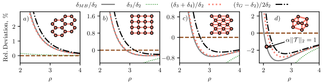
Figure 2: The solid line shows the MB effects, the small green dotted line the AT correction, the large orange dotted line shows four-body corrections added to the AT potential, the dashed dotted line shows the deviation between the sum of the reduced tangle of each of the $3N$ modes in the $N$ QDO system and the pairwise bonding energy, $(\tilde{\tau}_{G}-\delta_{2})/2$, with the factor of $1/2$ included as $(\tilde{\tau}_{G}-\delta_{2})/2\rightarrow\delta_{3}$ for $\rho\rightarrow\infty$. All the curves have been normalized by the pairwise bond energy and have been plotted as a function of the dimensionless nearest neighbour separation $\rho$. The horizontal dashed line separates positive and negative values. The following lattices are shown; a) $N=47\times 47\times 2$ honeycomb lattice b) $N=71\times 71$ square lattice c) $N=71\times 71$ triangular lattice d) $N=19\times 19\times 19$ cubic lattice. All lattices calculations have been preformed with open boundary conditions. The large circle in d), indicates the coupling strength where the binomial series used to derive Eq. (8) is no longer guaranteed to converge.

We consider three QDOs (trimer), see Fig. 1 $a)$ for a depiction of the setup. Fig. 1 $b)-c)$, show the maximal allowed pairwise tangle, for each pair of modes in the trimer groundstate, consistent with the associated monogamy inequalities. Note that QDO 2, due to the symmetry of the trimer, must share identical pairwise entanglement with QDO 3 and QDO 1.

Fig. 1 $d)$ shows how the parameter space of the trimer is partitioned into regions (separated by the dotted red line) where $\delta_{\tau_{G}}^{1,2}$ and $\delta_{\tau_{G}}^{2,3}$ are either enhanced (above) or suppressed (below). This boundary approximates the boundary formed by the locus of points separating the attractive and repulsive MB energy. For any $\rho\geq 2.3$ the deviation in $\theta$ value between the two boundaries is less than $1.2\%$ of the $\theta$ value where $\delta_{MB}=0$. We thus find that the sign of the MB energy, well matches, whether or not the monogamy constraint restricts the sum of the pairwise tangle, in the nearest neighbour subsystem.

Next we substantiate our numerical findings by analytically relating measures of the groundstate entanglement to the binding energy. We use the definition of the tangle to introduce the entanglement measure $\tilde{\tau}_{G}(i)=g(\tau_{G}(i))$, defined here as the reduced tangle, where $g(x)=x(1+\sqrt{x})^{2}/(1+2\sqrt{x})^{2}$. The function $g(x)$ is monotonically increasing for all positive $x$, ensuring the reduced tangle is an entanglement monotone under LOCC.

We derive an inequality capturing the relation and dependence of pairwise and many-body contributions to the binding energy and the distribution of the reduced tangle as follows (see SM for proofs),

$$\begin{split}\tilde{\tau}_{G}=\sum^{3N}_{i=1}\tilde{\tau}_{G}(i)\leq\sum^{\infty}_{k=2}(k-1)\delta_{k}.\end{split}$$ (8)

This upper bound is derived from the special form of the QDO Hamiltonian, having off-diagonal coupling solely between position operators as well as the positive constraint on the potential matrix, $V$. The latter constraint ensures the quadrature variances remain finite. In the SM we upper bound the sum over all pairs of $\tau^{\star}_{G}(i:j)$ in terms of the r.h.s of Eq. (8).

Fig. 1 $e)-f)$ shows the convergence to the bound in Eq. (8) for different couplings strengths. Fig. 1 $e)$ shows that for $\rho=2.6$, $\tilde{\tau}_{G}<\delta_{2}+2\delta_{3}+3\delta_{4}$, for both the linear and triangular geometries, where $\tilde{\tau}_{G}<\delta_{2}$ in the triangular case, whereas $\tilde{\tau}_{G}>\delta_{2}$ in the linear geometry. In comparison Fig. 1 $f)$, shows that for strong coupling, $\tilde{\tau}_{G}>\delta_{2}$, for both arrangements. Taking $\delta_{2}$ away from both sides of Eq. (8), shows that $\tilde{\tau}_{G}-\delta_{2}\leq\sum^{\infty}_{k=3}(k-1)\delta_{k}$. Comparing this bound with the definition of the MB energy and the form of $E$ in Eq. (3) explains the qualitative correspondence between the dashed-dotted black line in Fig. 1 $d)$ and the sign of $\delta_{MB}$, where the former divides the parameter space, into the regions where $\tilde{\tau}_{G}<\delta_{2}$ (below) and the regions where $\tilde{\tau}_{G}>\delta_{2}$.

In the limit of $\rho\rightarrow\infty$, the sign of $\tilde{\tau}_{G}-\delta_{2}$ and the MB effects tends toward being given by the sign of the AT potential. The solid horizontal line at $\theta=\theta_{0}$ in Fig. 1 d) divides the phase space into regions of repulsive (below) and attractive AT contributions. From Fig. 1 d), in the non-interacting limit, where $\rho\rightarrow\infty$, we find that $\delta_{\tau_{G}}^{1,2}(\theta_{0})\rightarrow 1$ (also $\delta_{\tau_{G}}^{2,3}(\theta_{0})\rightarrow 1$). The sign of the AT potential is therefore equivalent to whether the pairwise entanglement asymptotically behaves monogamously or promiscuously, in the nearest neighbour partition of the trimer.

The Gaussian state framework can be directly extended to arbitrary assemblies such as layered systems and 3D lattices, which we consider next. The features of the trimer, shown in Fig. 1 $d)$, can be used to explain the sign of the MB contributions in the more complex lattices, shown in Fig. 2. At weak coupling, the sign of the MB effects are determined by the AT potential in the lattices. The AT potential can be written as a sum over triplets (trimers) of QDOs, (see SM). The honeycomb lattice has a positive and negligible AT potential, following from where $\delta_{3}=0$ in Fig. 1 $d)$, where the primitive translation vectors of the honeycomb lattice form an angle of $2\pi/3$. In Fig. 2 $b)-d)$, where $\delta_{3}<0$, a sign change occurs at strong coupling and the MB effects become attractive. The sign change also occurs in Fig. 1 d), as a function of $\rho$, for all geometries where $\delta_{3}<0$.

Fig. 2, shows that $(\tilde{\tau}_{G}-\delta_{2})/2\approx\delta_{MB}$, on all the lattices at $\rho=4$, indicated by the overlap of the solid and dashed dotted lines. Furthermore $(\tilde{\tau}_{G}-\delta_{2})/2>\delta_{MB}$ for all the $\rho$ values shown. In addition in Fig. 1 $d)$, the dashed dotted line, where $\tilde{\tau}_{G}=\delta_{2}$, lies within the repulsive green region, where $\delta_{MB}<0$. This can be understood from a rearrangement of Eq. (8), as $(\tilde{\tau}_{G}-\delta_{2})/2\leq\delta_{3}+(3/2)\delta_{4}+...$, where Fig. 2 further shows that $\delta_{MB}\approx\delta_{3}+\delta_{4}$, on the lattices. The convergence to Eq. (8), for the different lattices, is presented in the SM.

Conclusion.- Here we have looked at dipolar bound systems, with the QDO model. We have shown numerically, for the paradigmatic trimer example and for a physically based parameter range, the monogamous or promiscuous behaviour of the entanglement distribution, directly correlates with whether MB effects are repulsive or attractive.

Our numerics are substantiated by a bound we derive between the reduced tangle, an entanglement monotone defined by a monogamous entanglement measure for Gaussian states, and the terms in a perturbative expansion of the interaction energy. This constitutes, to the best of our knowledge, the first analytically rigorous relation between an entanglement measure and the significant contribution to the chemical correlation energy, due to dispersion.

Arbitrary arrangements of $N$ QDOs, can be studied efficiently using our method, as it only requires diagonalizing $3N\times 3N$ matrices, which scales as $\mathcal{O}(N^{3})$. Hence, while the results here focus on model systems, the same prescription, upon appropriate parameterization of the QDOs, could be applied to realistic materials. This would provide a direct link between their physical and chemical properties and the amount of entanglement shared by their constituents. Concepts from quantum information theory thus provide a novel path for shedding light on important chemical problems Gori et al. (2023); Lee et al. (2023); Ding et al. (2020).

Declarations

• There are no competing interests.

• Code and data is freely available from the authors upon reasonable request.

Supplemental Material: A Quantum Information Perspective on Many-Body Dispersive Forces

I S1. General QDO Hamiltonian

The general dipole order QDO Hamiltonian in units of $\hbar\omega_{0}$ is

$$\begin{gathered}\hat{H}_{g}=\frac{1}{2}\sum^{N}_{\mu=1}|\boldsymbol{\hat{\mathcal{P}}}_{\mu}|^{2}+\frac{1}{2}\sum^{N}_{\mu=1}|\boldsymbol{\hat{\chi}}_{\mu}|^{2}\frac{\omega^{2}_{\mu}}{\omega^{2}_{0}}+\\ \sum^{N}_{\mu>\xi}\frac{\omega_{\mu}\omega_{\xi}}{\omega^{2}_{0}}\sqrt{\alpha_{\mu}}\sqrt{\alpha_{\xi}}\boldsymbol{\hat{\chi}}_{\mu}e^{T}_{\mu}\mathcal{T}e_{\xi}\boldsymbol{\hat{\chi}}_{\xi},\end{gathered}$$ (S1)

where $\boldsymbol{\hat{\chi}}_{\mu}=\boldsymbol{\hat{r}}_{\mu}\sqrt{\omega_{0}m/\hbar}$, $\boldsymbol{\hat{\mathcal{P}}}_{\mu}=\boldsymbol{\hat{p}}_{\mu}/\sqrt{\hbar m\omega_{0}}$. Here $\omega_{0}$ is a reference frequency and $\alpha_{\mu}=q^{2}_{\mu}/(m_{\mu}\omega^{2}_{\mu}4\pi\epsilon_{0})$ is the polarizability of QDO $\mu$.

The general dispersive binding energy is given by

$$E^{g}=\frac{3}{2}\sum^{N}_{\mu=1}\frac{\omega_{\mu}}{\omega_{0}}-\frac{1}{2}\sum^{3N}_{i=1}\sqrt{\lambda^{g}_{i}},$$ (S2)

where $\lambda^{g}_{i}$ are the eigenvalues of the matrix $V^{g}$ where $e^{T}_{\mu}V^{g}e_{\mu}=(\omega^{2}_{\mu}/\omega^{2}_{0})\mathds{1}_{3}$ and $e^{T}_{\mu}V^{g}e_{\xi}=\frac{\omega_{\mu}\omega_{\xi}}{\omega^{2}_{0}}\sqrt{\alpha_{\mu}}\sqrt{\alpha_{\xi}}\boldsymbol{\hat{\chi}}_{\mu}e^{T}_{\mu}\mathcal{T}e_{\xi}$, given $\mu\neq\xi$. Note that $e_{\mu}$ as well as $\mathcal{T}$ have been defined in the main-text. The general covariance matrix is thus computable in terms of the matrix $V^{g}$, as $\gamma^{g}_{0}=(V^{g})^{-1/2}\oplus(V^{g})^{1/2}$. Here $((V^{g})^{-1/2})_{ij}=\langle\hat{\chi}_{i}\hat{\chi}_{j}\rangle$ and $((V^{g})^{1/2})_{ij}=\langle\hat{\mathcal{P}}_{i}\hat{\mathcal{P}}_{j}\rangle$. The more general CM $\gamma^{g}_{0}$, replaces the CM in the main-text, when numerically studying arbitrarily parameterized QDOs. Extracting the necessary entanglement information follows the same procedure as defined in the main-text, but instead now using the elements of $\gamma^{g}_{0}$.

II S2. Axilrod-Teller formulae

The AT correction, looked at in the main-text, can be further written for $N\geq 3$ Donchev (2006) as a sum over triplets of QDOs,

$$\delta_{3}=\frac{-\alpha^{3}}{32}\mathrm{tr}(\mathcal{T}^{3})=\frac{-9\alpha^{3}}{16}\sum^{N}_{\o>\xi>\mu=1}\frac{[1+3\mathrm{cos}(\theta_{\mu\xi})\mathrm{cos}(\theta_{\mu\o})\mathrm{cos}(\theta_{\xi\o})]}{R^{3}_{\mu\xi}R^{3}_{\mu\o}R^{3}_{\xi\o}}.$$ (S3)

The angles $\theta_{\mu\xi}$ is given by,

$$\mathrm{cos}(\theta_{\mu\xi})=\frac{-R^{2}_{\mu\xi}+R^{2}_{\mu\o}+R^{2}_{\xi\o}}{2R_{\mu\o}R_{\xi\o}}.$$ (S4)

III S3. Properties of the groundstate CM

Lemma. 1 $(V^{1/2})_{ii}\leq 1\>\forall i\in\{1,2,...,3N\}$.

Proof. The matrix $V$ is a symmetric matrix, $V=V^{T}$, with positive eigenvalues $\lambda$. It is therefore diagonalized by a orthogonal matrix, $O$ ($OO^{T}=\mathds{1}$). The diagonal elements of the matrix square root of $V$ are given by

$$(V^{1/2})_{ii}=\sum^{3N}_{j=1}O^{2}_{ij}\sqrt{\lambda_{j}},\quad{}\sum^{3N}_{j=1}O^{2}_{ij}=1.$$ (S5)

The diagonal elements of $V^{1/2}$ are given by a convex combination of the square root of the eigenvalues of $V$. We apply Jensen’s inequality Hansen and Pedersen (2003), which states that

$$\left(\sum^{3N}_{j=1}O^{2}_{ij}\sqrt{\lambda_{j}}\right)^{2}\leq\sum^{3N}_{j=1}O^{2}_{ij}\left(\sqrt{\lambda_{j}}\right)^{2},$$ (S6)

which gives the result, as by definition,

$$\sum^{3N}_{j=1}O^{2}_{ij}\lambda_{j}=V_{ii}=1.$$ (S7)

Lemma. 2 The dispersive binding energy is always net attractive , i.e $E\geq 0$.

Proof. This follows from lemma. 1, as the bond energy is

$$E=\frac{3}{2}N-\frac{1}{2}\sum^{3N}_{i=1}(V^{1/2})_{ii},$$ (S8)

where $E\geq 0$, directly follows from the fact that $(V^{1/2})_{ii}\leq 1\forall i\in\{1,..,3N\}$.

Lemma. 3 $(V^{-1/2})_{ii}\geq[(V^{1/2})_{ii}]^{-1},\>\forall i\in\{1,..,3N\}.$

Proof. As $V^{1/2}$ is the unique symmetric positive definite matrix such that $(V^{1/2})^{2}=V$ Horn and Johnson (2012), there is a unique symmetric positive matrix $C$ where $V^{1/2}=CC$ and thus also $V^{-1/2}=(C^{-1})^{2}$. Note that as $C$ is a symmetric matrix, $C_{ij}=C_{ji}$ and $(C^{-1})_{ij}=(C^{-1})_{ji}$. We can thus employ the Cauchy-Schwartz inequality to complete the proof,

$$\underbrace{\left(\sum^{3N}_{j=1}C_{ij}(C^{-1})_{ji}\right)^{2}}_{=1}\leq\underbrace{\left(\sum^{3N}_{j=1}C_{ij}^{2}\right)}_{(V^{1/2})_{ii}}\underbrace{\left(\sum^{3N}_{j=1}(C^{-1})^{2}_{ji}\right)}_{{(V^{-1/2})_{ii}}}.$$ (S9)

IV S4. Symplectic diagonalization

Supplementary Figure 1: AT potential in the trimer at $\rho=2.60$ (see main-text for description). The orange crosses show $\delta_{3}$ computed via the R.H.S of Eq. (S3), whereas the solid grey curve shows $\delta_{3}$ computed by the L.H.S of Eq. (S3)

A general quadratic bosonic Hamiltonian can always be written as

$$\hat{H}=\frac{1}{2}\boldsymbol{\hat{q}}^{T}H\boldsymbol{\hat{q}},\quad{}H>0,$$ (S10)

where $\boldsymbol{\hat{q}}=(\hat{\chi}_{1},...,\hat{\chi}_{d},\hat{\mathcal{P}}_{1},...,\hat{\mathcal{P}}_{d})^{T}$ and $d$ is the number of modes in the system. The groundstate energy can be found variationally in terms of the CM as

$$E_{0}=\mathrm{inf}_{\gamma}\frac{1}{4}\rm{tr}(\gamma H),\quad{}\mathrm{with}\quad{}\gamma+i\sigma\geq 0,$$ (S11)

where the matrix $\sigma$ encodes the commutation relations,

$$\sigma=\begin{bmatrix}0&\mathds{1}\\ -\mathds{1}&0\end{bmatrix}.$$ (S12)

The constraint $\gamma+\rm{i}\sigma\geq 0$, enforces the Heisenberg uncertainty principle. A matrix which preserves $\sigma$ and therefore the commutation relations under a transformation is a symplectic matrix Serafini (2017), belonging to the symplectic matrix group,

$$S\sigma S^{T}=\sigma\quad{}S\in\mathcal{S}_{p}(\mathrm{dim}(2d,\mathds{R}).$$ (S13)

Williamson’s theorem Williamson (1936) states there is always a symplectic matrix which brings $H$ into diagonal form,

$$SHS^{T}=\begin{pmatrix}\epsilon_{1}&0&\cdots&0&0\\ 0&\epsilon_{1}&\cdots&0&0\\ \vdots&\vdots&\ddots&\vdots&\vdots\\ 0&0&\cdots&\epsilon_{d}&0\\ 0&0&\cdots&0&\epsilon_{d}\end{pmatrix},$$ (S14)

where $\epsilon_{i}$ are the symplectic eigenvalues of $H$, each repeated once along the diagonal. The groundstate CM can be written as $\gamma_{0}=S^{T}S$ Schuch et al. (2006). From the unitary representation of the symplectic matrix, which brings $H$ into diagonal form, the groundstate energy is given by the sum of the unique symplectic eigenvalues Schuch et al. (2006); Serafini (2017),

$$E_{0}=\frac{1}{2}\sum^{d}_{i=1}\epsilon_{i}.$$ (S15)

V S5. Two mode tangle energy bound

The two mode ($d=2$) quadratic Hamiltonian, coupled in position operators is given by

$$\hat{H}=\frac{1}{2}\left(\hat{\chi}^{2}_{1}+\hat{\chi}^{2}_{2}+\hat{\mathcal{P}}^{2}_{1}+\hat{\mathcal{P}}^{2}_{2}\right)+\kappa\hat{\chi}_{1}\hat{\chi}_{2},\quad{}|\kappa|<1.$$ (S16)

In order for the positive definite constraint on the Hamiltonian matrix to be obeyed, $|\kappa|<1$. The Hamiltonian in Eq. (S16) is equivalent to the two mode Hamiltonian $\hat{H}_{ij}$, in the main-text, for $\kappa=\alpha\mathcal{T}_{ij}$.

The symplectic spectrum $\{\epsilon_{+},\epsilon_{-},\epsilon_{+},\epsilon_{-}\}$ is given by,

$$\epsilon_{\pm}=\sqrt{1\pm\kappa}.$$ (S17)

The two mode bond energy, describing the deviation between the groundstate energy at $\kappa=0$ and the groundstate energy at a finite $\kappa$ value is

$$E=1-\frac{\epsilon_{+}+\epsilon_{-}}{2}.$$ (S18)

The two mode groundstate correlation matrix, is given by

$$\gamma_{0}=\frac{1}{2}\begin{pmatrix}\epsilon^{-1}_{+}+\epsilon^{-1}_{-}&\epsilon^{-1}_{+}-\epsilon^{-1}_{-}\\ \epsilon^{-1}_{+}-\epsilon^{-1}_{-}&\epsilon^{-1}_{+}+\epsilon^{-1}_{-}\end{pmatrix}\oplus\begin{pmatrix}\epsilon_{+}+\epsilon_{-}&\epsilon_{+}-\epsilon_{-}\\ \epsilon_{+}-\epsilon_{-}&\epsilon_{+}+\epsilon_{-}\end{pmatrix},$$ (S19)

where $2\langle\hat{\chi}^{2}_{1}\rangle=2\langle\hat{\chi}^{2}_{2}\rangle=\epsilon^{-1}_{+}+\epsilon^{-1}_{-}$, $2\langle\hat{\chi}_{1}\hat{\chi}_{2}\rangle=\epsilon^{-1}_{+}-\epsilon^{-1}_{-}$, $2\langle\hat{\mathcal{P}}^{2}_{1}\rangle=2\langle\hat{\mathcal{P}}^{2}_{2}\rangle=\epsilon_{+}+\epsilon_{-}$ and $2\langle\hat{\mathcal{P}}_{1}\hat{\mathcal{P}}_{2}\rangle=\epsilon_{+}-\epsilon_{-}$.

From the definition of the Gaussian tangle in the main-text in Eq. (6) and using the form of the two mode CM defined in Eq. (S19),

$$\tau_{G}(1)=\tau_{G}(1:2)=\frac{1}{4}\left(\sqrt{\frac{\epsilon_{+}}{\epsilon_{-}}}-1\right)^{2},$$ (S20)

from which the definition of $\tau_{G}^{\mathrm{ref}}(i:j)$, given in the main-text, follows. Expanding Eq. (S20) and inserting Eq. (S18), leads to

$$2\tau_{G}(1:2)=\frac{\left(E-\sqrt{\epsilon_{+}}\sqrt{\epsilon_{-}}+1\right)}{\epsilon_{-}}.$$ (S21)

As $|\kappa|<1$, it is also the case that $\epsilon_{-}<1$ and $\sqrt{\epsilon_{+}}\sqrt{\epsilon_{-}}<1$. We are thus left with

$$2\tau_{G}(1:2)=\tau_{G}(1)+\tau_{G}(2)\geq E.$$ (S22)

VI S6. Mixed state Pairwise Tangle

The pairwise tangle, $\tau_{G}(i:j)$, quantifying the entanglement shared between modes $i$ and $j$ in a mixed two mode state, is elaborated on here. We define the following quantities, which uniquely capture the two mode entanglement; $a^{ii},b^{jj},c^{ij}_{+},c_{-}^{ij}$, with $c^{ij}_{+}\geq|c_{-}^{ij}|$ . These are required to satisfy the following equalities: $a^{ii}=\sqrt{\langle\hat{\chi}^{2}_{i}\rangle\langle\hat{P}_{i}^{2}\rangle}$, $b^{jj}=\sqrt{\langle\hat{\chi}^{2}_{j}\rangle\langle\hat{P}_{j}^{2}\rangle}$, $c^{ij}_{+}c_{-}^{ij}=\langle\hat{\chi}_{i}\hat{\chi}_{j}\rangle\langle\hat{P}_{i}\hat{P}_{j}\rangle$ and $(a^{ii}b^{jj}-(c^{ij}_{+})^{2})(a^{ii}b^{jj}-(c^{ij}_{-})^{2})=((\langle\hat{P}_{i}\hat{P}_{j}\rangle)^{2}-\langle\hat{P}_{i}^{2}\rangle\langle\hat{P}_{j}^{2}\rangle)((\langle\hat{\chi}_{i}\hat{\chi}_{j}\rangle)^{2}-\langle\hat{\chi}^{2}_{i}\rangle\langle\hat{\chi}^{2}_{j}\rangle)$. In addition the following inequalities must be satisfied: $a^{ii}\geq 1$, $b^{jj}\geq 1$ (which follows from lemma. 3 in S3), $a^{ii}b^{jj}-(c^{ij}_{\pm})^{2}\geq 1$ and $(a^{ii}b^{jj}-(c^{ij}_{+})^{2})(a^{ii}b^{jj}-(c^{ij}_{-})^{2})+1\geq(a^{ii})^{2}+(b^{jj})^{2}+2c^{ij}_{+}c^{ij}_{-}$. For notational convenience we will write $a^{ii},b^{jj},c^{ij}_{+},c_{-}^{ij}$ as $a,b,c_{+},c_{-}$, for here onwards. The pairwise tangle is then given by Hiroshima et al. (2007),

$$\tau_{G}(i:j)=f(\mathrm{min}_{0\leq\phi<2\pi}m(\phi)),$$ (S23)

where recall the definition of $f(x)$ given in the main-text. Here

$$m(\phi)=h^{2}_{1}(\phi)/h_{2}(\phi),$$ (S24)

$$h_{1}(\phi)=\xi_{-}+\sqrt{\eta^{*}}\cos(\phi),$$ (S25)

$$h_{2}(\phi)=2(ab-c^{2}_{-})(a^{2}+b^{2}+2c_{+}c_{-})-\\ (\zeta/\sqrt{\eta^{*}})\cos(\phi)+(a^{2}-b^{2})\sqrt{1-\xi^{2}_{+}/\eta^{*}}\sin(\phi)$$ (S26)

$$\xi_{\pm}=c_{+}(ab-c^{2}_{-})\pm c_{-}$$ (S27)

$$\eta^{*}=[a-b(ab-c^{2}_{-}][b-a(ab-c^{2}_{-}])]$$ (S28)

and

$$\zeta=2abc^{3}_{-}+(a^{2}+b^{2})c_{+}c^{2}_{-}+[a^{2}+b^{2}-2a^{2}b^{2}]c_{-}\\ -ab(a^{2}+b^{2}-2)c_{+}.$$ (S29)

VII S7. Three mode Hamiltonian and a low dimensional approximation

Using the truncated Fock state approach (see Anderson et al. (2022)), a quadratic $d$ mode Hamiltonian with coupling only between position modes — using only the first two Fock states i.e $|0\rangle$ and $|1\rangle$ — leads to the following $d$ qubit Hamiltonian,

$$\hat{H}^{q}_{d}=\frac{1}{2}\sum^{d}_{i=1}\left(2\mathds{1}^{i}_{2}-\sigma^{i}_{z}\right)+\sum^{d}_{j>i}w_{ij}\sigma^{i}_{x}\otimes\sigma^{j}_{x}.$$ (S30)

Here $\sigma^{i}_{z}$ ($\sigma^{i}_{x}$) is the $z$ ($x$) Pauli matrix, acting on the $i$th qubit, $w_{ij}$ is determined by the coupling strength between modes and $\otimes$ denotes the tensor product. The ground-state density matrix is a $2^{d}\times 2^{d}$ matrix, denoted by $\hat{\rho}^{d}$. For example when $d=2$, Eq. (S30) is a two qubit Hamiltonian, with $w_{12}=\kappa$. It’s $4\times 4$ groundstate density matrix is written as $\hat{\rho}^{2}$. The tangle between qubits 1 and 2, can be straightforwardly computed from the reduced density matrix, tracing out qubit 2, giving the $2\times 2$ reduced density matrix $\hat{\rho}^{2}_{2}$. The tangle between qubits 1 and 2 is given by Coffman et al. (2000),

$$\tau^{\mathrm{ref}}(1:2)=4\mathrm{Det}(\hat{\rho}^{2}_{1}).$$ (S31)

Analogously, the Gaussian tangle in the two mode pure state, denoted by $\tau_{G}^{\mathrm{ref}}(1:2)$, is given by Eq. (S20).

Here we will extend the Hamiltonian looked at in Eq. (S16). The three mode Hamiltonian we will consider here is

$$\hat{H}=\frac{1}{2}\left(\hat{\chi}^{2}_{1}+\hat{\chi}^{2}_{2}+\hat{\chi}^{2}_{3}+\hat{\mathcal{P}}^{2}_{1}+\hat{\mathcal{P}}^{2}_{2}+\hat{\mathcal{P}}^{2}_{3}\right)+\kappa\hat{\chi}_{1}\hat{\chi}_{2}+\kappa\beta\hat{\chi}_{1}\hat{\chi}_{3}+\kappa\hat{\chi}_{2}\hat{\chi}_{3},\quad{}|\kappa|<1,\beta\leq|\kappa|.$$ (S32)

Given $d=3$, $\hat{H}^{q}_{3}$ is a three qubit Hamiltonian, where $w_{12}=w_{23}=\kappa$ and $w_{13}=\beta\kappa$. The groundstate density matrix is given by $\hat{\rho}^{3}$. The monogamy inequality for distributed qubit entanglement, is given in terms of the tangle as

$$\tau(1)\geq\tau(1:2)+\tau(1:3),$$ (S33)

where $\tau(1)=4\mathrm{Det}(\hat{\rho}^{3}_{1})$, where $\hat{\rho}^{3}_{1}$ is a $2\times 2$ matrix, found by tracing out qubits 2 and 3. The associated monogamy inequality for the tripartite groundstate of Eq. (S32) is

$$\tau_{G}(1)\geq\tau_{G}(1:2)+\tau_{G}(1:3),$$ (S34)

following from the fact that $\tau_{G}(1)\geq\tau^{\star}_{G}(1:2)+\tau^{\star}_{G}(1:3)$, where $\tau^{\star}_{G}(i:j)$ is defined in the main-text and $\tau^{\star}_{G}(1:2)\geq\tau_{G}(1:2)$, $\tau^{\star}_{G}(1:3)\geq\tau_{G}(1:3)$.

In Fig. 2, we show how $\tau^{\star}_{G}(1:2)$ and $\tau(1:2)$ are modified, due to the tripartite interaction, setting $\beta=1/4$, and for positive and negative coupling $\kappa$. For negative $\kappa$ in Fig. 2 $a)$ , both $\tau^{\star}_{G}(1:2)>\tau^{\mathrm{ref}}_{G}(1:2)$ and $\tau(1:2)>\tau^{\mathrm{ref}}(1:2)$ for $\kappa^{-1/2}\geq 2$. In comparison at weak coupling in Fig. 2 $b)$, both $\tau^{\star}_{G}(1:2)<\tau^{\mathrm{ref}}_{G}(1:2)$ and $\tau(1:2)<\tau^{\mathrm{ref}}(1:2)$. Here, mode (qubit) 3 restricts the shared tangle between modes (qubits) 1 and 2. For increasing coupling strength, a sign change occurs in $\tau^{\star}_{G}(1:2)-\tau^{\mathrm{ref}}_{G}(1:2)$ but not in $\tau(1:2)-\tau^{\mathrm{ref}}(1:2)$.

Supplementary Figure 2: The solid orange curve is the tangle computed from solving Eq. (S32) exactly. The dashed dotted black line, follows from the truncated Fock state approximation, with Hamiltonian given in Eq. (S30) and $d=3$. Below the horizontal dashed line shows where the pairwise entanglement between 1 and 2 behaves monogamously whereas above shows the promiscuous behaviour.

VIII S8. Multipartite Tangle and Energy

From the definition of the tangle $\tau_{G}(i)$ and the reduced tangle $\tilde{\tau}_{G}(i)$, both given in the main-text, we can write

$$\tilde{\tau}_{G}=\frac{1}{4}\sum^{3N}_{i=1}\Delta_{i}=\sum^{3N}_{i=1}g(\tau_{G}(i)),$$ (S35)

where $\Delta_{i}=\langle\hat{\chi}^{2}_{i}\rangle\langle\hat{\mathcal{P}}^{2}_{i}\rangle-1$. By defining $\delta^{\chi}_{i}=\langle\hat{\chi}^{2}_{i}\rangle-1,\>\delta^{\mathcal{P}}_{i}=1-\langle\hat{\mathcal{P}}^{2}_{i}\rangle$, we write $\Delta_{i}$ as follows,

$$\Delta_{i}=\delta^{\chi}_{i}-\delta^{\mathcal{P}}_{i}-\delta^{\chi}_{i}\delta^{\mathcal{P}}_{i}.$$ (S36)

By using the unitary invariance of the trace operator and writing $\left(\lambda_{i}\right)^{\pm 1/2}=\left(1+\alpha t_{i}\right)^{\pm 1/2}$, the binomial expansion of $\left(\lambda_{i}\right)^{\pm 1/2}$ in small parameter $\alpha t_{i}$ is

$$\sum^{3N}_{i=1}\delta^{\chi}_{i}=\sum^{3N}_{i=1}\left(\left(\sqrt{\lambda_{i}}\right)^{-1}-1\right)=\sum^{\infty}_{k=2}{-0.5\choose k}\alpha^{k}\mathrm{tr}(\mathcal{T}^{k}),$$ (S37)

and

$$\sum^{3N}_{i=1}\delta^{\mathcal{P}}_{i}=\sum^{3N}_{i=1}\left(1-\sqrt{\lambda_{i}}\right)=-\sum^{\infty}_{k=2}{0.5\choose k}\alpha^{k}\mathrm{tr}(\mathcal{T}^{k}).$$ (S38)

By inserting Eq. (S37) and Eq. (S38) into Eq. (S36) and Eq. (S35), then simplifying the resultant expression we arrive at

$$\tilde{\tau}_{G}=\sum^{\infty}_{k=2}(k-1)\delta_{k}-\frac{1}{4}\sum^{3N}_{i=1}\delta^{\chi}_{i}\delta^{\mathcal{P}}_{i},$$ (S39)

where $\delta_{k}$ is defined in Eq. (3), in the main-text. The upper bound on $\tilde{\tau}_{G}$ in Eq. (8), follows from $\delta^{\chi}_{i}=\langle\hat{\chi}^{2}_{i}\rangle-1\geq 0$ and $\delta^{\mathcal{P}}_{i}=1-\langle\hat{\mathcal{P}}^{2}_{i}\rangle\geq 0$, both $\forall i\in\{1,..,3N\}$, due to a combination of lemma. 1 III and lemma. 3 in section III.

Supplementary Figure 3: Convergence to Eq. (8), given in the main-text, for the honeycomb lattice in a), e) and i), the square lattice in b), f) and j), the triangular lattice in c), g) and k) and the cubic lattice in d), h) and l). Panels a)-d), are at $\rho=4$, e)-h) at $\rho=2.93$ and i)-l) are at $\rho=2.37$. The dashed horizontal line shows the value of $\tilde{\tau}_{G}$ for the correspondent $\rho$ value and lattice.

Given that $g(x)$ is a subadditive function i.e $g(x+y)\leq g(x)+g(y)$ (see section VIII.),

$$g\left(\tau_{G}=\sum^{3N}_{i=1}\tau_{G}(i)\right)\leq\sum^{3N}_{i=1}g(\tau_{G}(i))=\tilde{\tau}_{G}.$$ (S40)

This sub-additive property of $g(x)$ can be extend to the inequality in Eq. (8) in the main-text,

$$g(\tau_{G})\leq\tilde{\tau}_{G}\leq\sum^{\infty}_{k=2}(k-1)\delta_{k}.$$ (S41)

The sum of each of the $3N$ monogamy inequalities Hiroshima et al. (2007) in the QDO ensemble are given by

$$\sum^{3N}_{i=1}\tau_{G}(i)\geq\sum^{3N}_{\begin{subarray}{c}i,j=1\\ j\neq i\end{subarray}}\underbrace{f((-\langle\hat{\chi}_{i}\hat{\chi}_{j}\rangle\langle\hat{\mathcal{P}}_{i}\hat{\mathcal{P}}_{j}\rangle)}_{\tau^{*}_{G}(i:j)}\geq\\ \sum^{3N}_{\begin{subarray}{c}i,j=1\\ j\neq i\end{subarray}}\tau_{G}(i:j),$$ (S42)

with $f(x)$ defined in the main-text. Inserting (S42) into (S41), we get

$$g\left(\sum^{3N}_{\begin{subarray}{c}i,j=1\\ j\neq i\end{subarray}}\tau^{*}_{G}(i:j)\right)\leq\sum^{\infty}_{k=2}(k-1)\delta_{k}.$$ (S43)

In Fig. 3, we show the convergence to the upper bound on the reduced tangle given in the main-text in Eq. (8), for the same four crystal lattices, investigated numerically in the main-text. We further consider the same setups (number of QDOs and open boundary conditions) as in the main-text.

IX S9. Properties of $g(x)$

lemma. 4 $g(y)\geq g(x)$, given $y\geq x\geq 0$.

Proof. The derivative of $g(x)$ is non-negative for any positive $x$,

$$\frac{\partial\left(g(x)\right)}{\partial_{x}}=\frac{1+\sqrt{x}(1+2\sqrt{x}+2x)}{(1+2\sqrt{x})^{3}}\geq 0,\quad{}\forall x\geq 0.$$ (S44)

lemma. 5 $g(x+y)\leq g(x)+g(y)$, given $x,y\geq 0$

Proof. The derivative of $g(x)/x$ is always negative for any positive $x$,

$$\frac{\partial\left(\frac{g(x)}{x}\right)}{\partial_{x}}=\frac{-(1+\sqrt{x})}{(1+2\sqrt{x})^{3}\sqrt{x}}\leq 0,\quad{}\mathrm{given}\quad{}x\geq 0.$$ (S45)

As a result for positive $x$ and $y$, we can write,

$$\frac{g(y)}{y}\leq\frac{g(x)}{x},\quad{}\mathrm{if}\quad{}0\leq x\leq y.$$ (S46)

Thus,

$$g(cx)\leq cg(x)\quad{}c\geq 1,$$ (S47)

because $c$ can always be written as $c=y/x$. As a result the inequality in Eq. (S47) follows from Eq. (S46). The subadditivity of $g(x)$ follows from inserting $c_{1}=1+y/x$ into $c$ in Eq. (S47) and $c_{2}=1+x/y$ into $c$ in Eq. (S47) also. By adding and simplifying the resultant two inequalities, Eq. (S47) implies $g(x+y)\leq g(x)+g(y)$, for positive $x$ and $y$.

References

- Stone (2013) A. Stone, The Theory of Intermolecular Forces (Oxford University Press, 2013).
- Hirschfelder (2009) J. O. Hirschfelder, Intermolecular Forces, Volume 12, Vol. 12 (John Wiley & Sons, 2009).
- London (1930) F. London, Zeitschrift für Physik 63, 245 (1930).
- Hermann et al. (2017a) J. Hermann, R. A. DiStasio Jr, and A. Tkatchenko, Chemical Reviews 117, 4714 (2017a).
- Grimme (2011) S. Grimme, Wiley Interdisciplinary Reviews: Computational Molecular Science 1, 211 (2011).
- DiStasio et al. (2014) R. A. DiStasio, V. V. Gobre, and A. Tkatchenko, Journal of Physics: Condensed Matter 26, 213202 (2014).
- Pastorczak et al. (2017) E. Pastorczak, J. Shen, M. Hapka, P. Piecuch, and K. Pernal, Journal of Chemical Theory and Computation 13, 5404 (2017).
- Von Lilienfeld et al. (2004) O. A. Von Lilienfeld, I. Tavernelli, U. Rothlisberger, and D. Sebastiani, Physical Review Letters 93, 153004 (2004).
- French et al. (2010) R. H. French, V. A. Parsegian, R. Podgornik, R. F. Rajter, A. Jagota, J. Luo, D. Asthagiri, M. K. Chaudhury, Y.-m. Chiang, S. Granick, et al., Reviews of Modern Physics 82, 1887 (2010).
- Dzyaloshinskii et al. (1961) I. E. Dzyaloshinskii, E. M. Lifshitz, and L. P. Pitaevskii, Soviet Physics Uspekhi 4, 153 (1961).
- Stillinger and Weber (1985) F. H. Stillinger and T. A. Weber, Physical Review B 31, 5262 (1985).
- Axilrod (1951) B. Axilrod, The Journal of Chemical Physics 19, 724 (1951).
- Jansen (1964) L. Jansen, Physical Review 135, A1292 (1964).
- Rösel et al. (2017) S. Rösel, H. Quanz, C. Logemann, J. Becker, E. Mossou, L. Cañadillas-Delgado, E. Caldeweyher, S. Grimme, and P. R. Schreiner, Journal of the American Chemical Society 139, 7428 (2017).
- Kronik and Tkatchenko (2014) L. Kronik and A. Tkatchenko, Accounts of Chemical Research 47, 3208 (2014).
- Wagner and Schreiner (2015) J. P. Wagner and P. R. Schreiner, Angewandte Chemie International Edition 54, 12274 (2015).
- DiStasio Jr et al. (2012) R. A. DiStasio Jr, O. A. von Lilienfeld, and A. Tkatchenko, Proceedings of the National Academy of Sciences 109, 14791 (2012).
- Stöhr and Tkatchenko (2019) M. Stöhr and A. Tkatchenko, Science Advances 5, eaax0024 (2019).
- Tkatchenko et al. (2011) A. Tkatchenko, M. Rossi, V. Blum, J. Ireta, and M. Scheffler, Physical Review Letters 106, 118102 (2011).
- Autumn et al. (2002) K. Autumn, M. Sitti, Y. A. Liang, A. M. Peattie, W. R. Hansen, S. Sponberg, T. W. Kenny, R. Fearing, J. N. Israelachvili, and R. J. Full, Proceedings of the National Academy of Sciences 99, 12252 (2002).
- Singla et al. (2021) S. Singla, D. Jain, C. M. Zoltowski, S. Voleti, A. Y. Stark, P. H. Niewiarowski, and A. Dhinojwala, Science Advances 7, eabd9410 (2021).
- Ambrosetti et al. (2014) A. Ambrosetti, D. Alfè, R. A. DiStasio Jr, and A. Tkatchenko, The Journal of Physical Chemistry Letters 5, 849 (2014).
- Tkatchenko et al. (2012) A. Tkatchenko, R. A. DiStasio Jr, R. Car, and M. Scheffler, Physical Review Letters 108, 236402 (2012).
- Misquitta et al. (2014) A. J. Misquitta, R. Maezono, N. D. Drummond, A. J. Stone, and R. J. Needs, Physical Review B 89, 045140 (2014).
- Shtogun and Woods (2010) Y. V. Shtogun and L. M. Woods, The Journal of Physical Chemistry Letters 1, 1356 (2010).
- Hermann et al. (2017b) J. Hermann, D. Alfe, and A. Tkatchenko, Nature Communications 8, 14052 (2017b).
- Deringer and Csanyi (2016) V. L. Deringer and G. Csanyi, The Journal of Physical Chemistry C 120, 21552 (2016).
- Kim et al. (2016) W. J. Kim, M. Kim, E. K. Lee, S. Lebegue, and H. Kim, The Journal of Physical Chemistry Letters 7, 3278 (2016).
- Marom et al. (2013) N. Marom, R. A. DiStasio Jr, V. Atalla, S. Levchenko, A. M. Reilly, J. R. Chelikowsky, L. Leiserowitz, and A. Tkatchenko, Angewandte Chemie International Edition 52, 6629 (2013).
- Reilly and Tkatchenko (2014) A. M. Reilly and A. Tkatchenko, Physical Review Letters 113, 055701 (2014).
- Reilly and Tkatchenko (2013) A. M. Reilly and A. Tkatchenko, The Journal of Physical Chemistry Letters 4, 1028 (2013).
- Rościszewski et al. (2000) K. Rościszewski, B. Paulus, P. Fulde, and H. Stoll, Physical Review B 62, 5482 (2000).
- Maaravi et al. (2017) T. Maaravi, I. Leven, I. Azuri, L. Kronik, and O. Hod, The Journal of Physical Chemistry C 121, 22826 (2017).
- Terhal (2004) B. M. Terhal, IBM Journal of Research and Development 48, 71 (2004).
- Adesso and Illuminati (2006) G. Adesso and F. Illuminati, International Journal of Quantum Information 4, 383 (2006).
- Horodecki et al. (2009) R. Horodecki, P. Horodecki, M. Horodecki, and K. Horodecki, Reviews of modern physics 81, 865 (2009).
- Coffman et al. (2000) V. Coffman, J. Kundu, and W. K. Wootters, Physical Review A 61, 052306 (2000).
- Osborne and Verstraete (2006) T. J. Osborne and F. Verstraete, Physical Review Letters 96, 220503 (2006).
- Hiroshima et al. (2007) T. Hiroshima, G. Adesso, and F. Illuminati, Physical Review Letters 98, 050503 (2007).
- Wolf et al. (2003) M. M. Wolf, F. Verstraete, and J. I. Cirac, International Journal of Quantum Information 1, 465 (2003).
- Pawłowski (2010) M. Pawłowski, Physical Review A 82, 032313 (2010).
- Lloyd and Preskill (2014) S. Lloyd and J. Preskill, Journal of High Energy Physics 2014, 1 (2014).
- Seevinck (2010) M. P. Seevinck, Quantum Information Processing 9, 273 (2010).
- Koashi and Winter (2004) M. Koashi and A. Winter, Physical Review A 69, 022309 (2004).
- O’Connor and Wootters (2001) K. M. O’Connor and W. K. Wootters, Physical Review A 63, 052302 (2001).
- Adesso et al. (2007) G. Adesso, M. Ericsson, and F. Illuminati, Physical Review A 76, 022315 (2007).
- Adesso and Illuminati (2007) G. Adesso and F. Illuminati, Journal of Physics A: Mathematical and Theoretical 40, 7821 (2007).
- Ferraro et al. (2007) A. Ferraro, A. García-Saez, and A. Acín, Physical Review A 76, 052321 (2007).
- Wang et al. (2021) Y. Wang, P. Knowles, and J. Wang, Physical Review A 103, 062808 (2021).
- Wang and Baerends (2022) J. Wang and E. J. Baerends, Physical Review Letters 128, 013001 (2022).
- Cipcigan et al. (2019) F. Cipcigan, J. Crain, V. Sokhan, and G. J. Martyna, Reviews of Modern Physics 91, 025003 (2019).
- Jones et al. (2013a) A. Jones, F. Cipcigan, V. Sokhan, J. Crain, and G. Martyna, Physical Review Letters 110, 227801 (2013a).
- Vaccarelli et al. (2021) O. Vaccarelli, D. V. Fedorov, M. Stöhr, and A. Tkatchenko, Physical Review Research 3, 033181 (2021).
- Bade (1957) W. Bade, The Journal of Chemical Physics 27, 1280 (1957).
- Wang and Jordan (2001) F. Wang and K. Jordan, The Journal of Chemical Physics 114, 10717 (2001).
- Jones et al. (2013b) A. P. Jones, J. Crain, V. P. Sokhan, T. W. Whitfield, and G. J. Martyna, Physical Review B 87, 144103 (2013b).
- Donchev (2006) A. Donchev, The Journal of Chemical Physics 125, 074713 (2006).
- Cipcigan et al. (2016) F. S. Cipcigan, V. P. Sokhan, J. Crain, and G. J. Martyna, Journal of Computational Physics 326, 222 (2016).
- London (1937) F. London, Transactions of the Faraday Society 33, 8b (1937).
- Sparnaay (1959) M. Sparnaay, Physica 25, 217 (1959).
- Hirschfelder et al. (1964) J. O. Hirschfelder, C. F. Curtiss, and R. B. Bird, Molecular theory of gases and liquids (1964).
- Cao and Berne (1992) J. Cao and B. Berne, The Journal of Chemical Physics 97, 8628 (1992).
- Khabibrakhmanov et al. (2023) A. Khabibrakhmanov, D. V. Fedorov, and A. Tkatchenko, Journal of Chemical Theory and Computation (2023).
- Jeziorski et al. (1994) B. Jeziorski, R. Moszynski, and K. Szalewicz, Chemical Reviews 94, 1887 (1994).
- Kim et al. (2006) H.-Y. Kim, J. O. Sofo, D. Velegol, M. W. Cole, and A. A. Lucas, The Journal of chemical physics 124 (2006).
- Langbein (1971) D. Langbein, Journal of Physics and Chemistry of Solids 32, 133 (1971).
- Renne and Nijboer (1967) M. Renne and B. Nijboer, Chemical Physics Letters 1, 317 (1967).
- Axilrod and Teller (1943) B. Axilrod and E. Teller, The Journal of Chemical Physics 11, 299 (1943).
- Weedbrook et al. (2012) C. Weedbrook, S. Pirandola, R. García-Patrón, N. J. Cerf, T. C. Ralph, J. H. Shapiro, and S. Lloyd, Reviews of Modern Physics 84, 621 (2012).
- Schuch et al. (2006) N. Schuch, J. I. Cirac, and M. M. Wolf, Communications in mathematical physics 267, 65 (2006).
- Wolf et al. (2004a) M. M. Wolf, F. Verstraete, and J. I. Cirac, Physical Review Letters 92, 087903 (2004a).
- Serafini (2017) A. Serafini, Quantum continuous variables: a primer of theoretical methods (CRC press, 2017).
- Dereziński (2017) J. Dereziński, Journal of Mathematical Physics 58, 121101 (2017).
- Colpa (1978) J. Colpa, Physica A: Statistical Mechanics and its Applications 93, 327 (1978).
- Van Hemmen (1980) J. Van Hemmen, Zeitschrift für Physik B Condensed Matter 38, 271 (1980).
- Maldonado (1993) O. Maldonado, Journal of Mathematical Physics 34, 5016 (1993).
- Plenio et al. (2005) M. B. Plenio, J. Eisert, J. Dreissig, and M. Cramer, Physical Review Letters 94, 060503 (2005).
- Cramer et al. (2006) M. Cramer, J. Eisert, M. B. Plenio, and J. Dreissig, Physical Review A 73, 012309 (2006).
- Giedke et al. (2003) G. Giedke, M. M. Wolf, O. Krüger, R. F. Werner, and J. I. Cirac, Physical review letters 91, 107901 (2003).
- Giedke et al. (2001) G. Giedke, B. Kraus, M. Lewenstein, and J. Cirac, Physical Review Letters 87, 167904 (2001).
- Adesso et al. (2014) G. Adesso, S. Ragy, and A. R. Lee, Open Systems & Information Dynamics 21, 1440001 (2014).
- Manuceau and Verbeure (1968) J. Manuceau and A. Verbeure, Communications in Mathematical Physics 9, 293 (1968).
- Holevo (1971) A. Holevo, Theor. Math. Phys 6, 3 (1971).
- Audenaert et al. (2002) K. Audenaert, J. Eisert, M. B. Plenio, and R. F. Werner, Physical Review A 66, 042327 (2002).
- Amico et al. (2008) L. Amico, R. Fazio, A. Osterloh, and V. Vedral, Reviews of modern physics 80, 517 (2008).
- Vidal and Werner (2002) G. Vidal and R. F. Werner, Physical Review A 65, 032314 (2002).
- Wolf et al. (2004b) M. M. Wolf, G. Giedke, O. Krüger, R. F. Werner, and J. I. Cirac, Physical Review A 69, 052320 (2004b).
- Adesso and Illuminati (2005) G. Adesso and F. Illuminati, Physical Review A 72, 032334 (2005).
- Gori et al. (2023) M. Gori, P. Kurian, and A. Tkatchenko, Nature Communications 14, 8218 (2023).
- Lee et al. (2023) S. Lee, J. Lee, H. Zhai, Y. Tong, A. M. Dalzell, A. Kumar, P. Helms, J. Gray, Z.-H. Cui, W. Liu, et al., Nature Communications 14, 1952 (2023).
- Ding et al. (2020) L. Ding, S. Mardazad, S. Das, S. Szalay, U. Schollwöck, Z. Zimborás, and C. Schilling, Journal of Chemical Theory and Computation 17, 79 (2020).
- Hansen and Pedersen (2003) F. Hansen and G. K. Pedersen, Bulletin of the London Mathematical Society 35, 553 (2003).
- Horn and Johnson (2012) R. A. Horn and C. R. Johnson, Matrix A mnalysis (Cambridge university press, 2012).
- Williamson (1936) J. Williamson, American Journal of Mathematics 58, 141 (1936).
- Anderson et al. (2022) L. W. Anderson, M. Kiffner, P. K. Barkoutsos, I. Tavernelli, J. Crain, and D. Jaksch, Physical Review A 105, 062409 (2022).