Configuring Transmission Thresholds in IIoT Alarm Scenarios for Energy-Efficient Event Reporting

Abstract

Industrial Internet of Things (IIoT) applications involve real-time monitoring, detection, and data analysis. This is challenged by the intermittent activity of IIoT devices and their limited battery capacity. Indeed, the former issue makes resource scheduling and/or random access difficult, while the latter constrains IIoT devices’ lifetime and efficient operation. In this paper, we address interconnected aspects of these issues. Specifically, we focus on extending the battery life of IIoT devices sensing events/alarms by minimizing the number of unnecessary transmissions. Note that when multiple devices access the channel simultaneously, there are collisions, potentially leading to retransmissions, thus reducing energy efficiency. We propose a threshold-based transmission-decision policy based on the sensing quality and the network spatial deployment. We optimize the transmission thresholds using several approaches such as successive convex approximation, block coordinate descent methods, Voronoi diagrams, explainable machine learning, and algorithms based on natural selection and social behavior. Besides, we propose a new approach that reformulates the optimization problem as a $\displaystyle Q$-learning solution to promote adaptability to system dynamics. Through numerical evaluation, we demonstrate significant performance enhancements in complex IIoT environments, thus validating the practicality and effectiveness of the proposed solutions. We show that Q-learning performs the best, while the block coordinate descending method incurs the worst performance. Additionally, we compare the proposed methods with a benchmark assigning the same threshold to all the devices for transmission decision. Notably, in low-density scenarios, all the proposed methods outperform the benchmark. On the other hand, successive convex approximation, Voronoi-(i), the K-nearest neighbors-based, and Q-learning outperform the benchmark, while the remaining methods attain similar performance in high-density scenarios. Compared to the benchmark, up to 94% and 60% reduction in power consumption are achieved in low-density and high-density scenarios, respectively.

I Introduction

The Industrial Internet of Things (IIoT) aims to connect Industry 4.0 and thus support predictive maintenance, asset tracking, smart manufacturing, energy management, environmental monitoring, health and safety monitoring, remote control, smart grid management, and agricultural automation [1]. These applications enhance efficiency, safety, and sustainability across several industries, e.g., manufacturing, agriculture, energy, and logistics. Indeed, by incorporating intelligent attributes, including the utilization of real-time data and automation for process optimization and decision-making, IIoT networks allow cyber-physical systems to operate proactively and efficiently [2].

IIoT networks are steadily evolving, driving massive data collection, analysis, and exploitation for control and sensing [3]. In addition, the corresponding applications are often latency-sensitive and handle large amounts of IIoT entities sharing scarce communication resources, e.g., time and bandwidth, resulting in severe co-channel interference. Unfortunately, coordinating the transmissions to mitigate the interference incurs significant overheads, especially because the payload size in IIoT is usually small [4]. Moreover, the sporadic activation of devices leads to highly inefficient coordination. Balancing resource scheduling without prior knowledge about when transmission resources are required and managing interference in large IIoT networks pose significant challenges [5]. Additionally, due to the limited battery capacity of IIoT devices (IIoTDs), improving energy efficiency and incorporating energy harvesting sources are crucial [6].

Note that the spatial arrangement of nodes in an IIoT network significantly impacts event detection accuracy and the effectiveness of alarm notifications. Indeed, one can enhance coverage, minimize blind spots, and optimize data transmission, thereby improving the overall efficiency of the network, by strategically deploying the IIoTDs [7]. Also, one can leverage available information on the spatial correlation among devices to enhance transmission policies upon an event triggering. For instance, tools such as Voronoi diagrams can help identify specific coverage areas for individual IIoTDs within a given space, aiding in spatial analysis [8]. Specifically, a clustering-based distributed learning solution for a medium access scheme is proposed in [6] to tackle the problem where a set of sensors may communicate a joint observation. The complexity lies in the limited signaling and shared information constraints, distinct from related research on exploiting sensor activity correlations or reliable alarm message transmission. In [9], the authors propose a novel channel scheduling method by leveraging the spatial correlation between device activations. Integrating spatial correlation information and employing clustering-based techniques offer promising avenues to optimize transmission policies and enhance the system’s energy efficiency and successful event detection.

Data-driven techniques are also suggested, e.g., in [10, 11, 12, 13, 14]. The authors in [10] propose a security framework that correlates activity across space and time to detect transmission patterns using data mining and supervised machine learning (ML), reaching 99% accuracy. In [11], the authors employ data capturing the correlations between devices to develop a random forest-based predictor for energy consumption in solar-powered nodes, leading to a 14% reduction in prediction error. The age-of-information (freshness of information) optimization problem is tackled using spatial correlations among IoT devices in [12]. The authors in [13] present a framework for deriving high-level industrial events from low-level raw data streams, which can be used for online correlation analysis with high-level process events into a process event log. Meanwhile, in [14], a statistical model is proposed for joint sensor identification and channel estimation using the least absolute shrinkage and selection operator joined to the orthogonal matching pursuit.

Despite the previous IIoT-related research projects, complex issues such as scalability, resource efficiency, and energy efficiency remain open challenges in implementing correlation-based strategies effectively [5]. Addressing these issues is essential to fully optimize IoT connectivity performance as illustrated in this work.

TABLE I: List of Symbols

Symbol	Description
$\displaystyle d_{i,j}$	Distance between $\displaystyle i^{\text{th}}$ event and an IIoTD $\displaystyle j$ at ($\displaystyle x_{j},y_{j}$)
$\displaystyle r_{j,h}$	Distance between two IIoTDs at ($\displaystyle x_{j},y_{j}$) and ($\displaystyle x_{h},y_{h}$)
$\displaystyle\mathbb{E}(\cdot)$	Expected value operator
$\displaystyle f_{X}(\cdot)$, $\displaystyle F_{X}(\cdot)$	PDF∗ and CDF∗ of random variable $\displaystyle X$
$\displaystyle g$	Maximum number of iterations for the algorithms
$\displaystyle\mathcal{J}$	Set of IIoTDs
$\displaystyle M$	Number of clusters in k-nearest neighbors
P	Transition probability from inactive to active state
$\displaystyle p(\cdot)$	Sensing power function
$\displaystyle P_{\text{col}}$	Collision probability
$\displaystyle P_{\text{e}}$	Error probability
$\displaystyle P_{\text{miss}}$	Miss-detection probability
$\displaystyle\Pr\left(A_{j}\right)$	Steady-state probability of IIoTD $\displaystyle j^{th}$ being active
$\displaystyle\Pr\left(A_{j}|A_{h}\right)$	Probability of IIoTD $\displaystyle j^{th}$ active if IIoTD $\displaystyle h^{th}$ is active
$\displaystyle Q(\cdot)$	Lookup $\displaystyle Q$-table
$\displaystyle S$	System space
$\displaystyle(s,a)$	State-action pair
$\displaystyle\mathcal{T}(\cdot)$	First-order Taylor serie approximation operator
$\displaystyle W(\cdot)$	Expected power consumption per IIoTD
$\displaystyle\alpha$	Probability of event occurrence
$\displaystyle\beta$	Cardinality of population vector in GA∗
$\displaystyle\xi$	Network area
$\displaystyle\eta$	Control factor sensitivity for a given distance
$\displaystyle\boldsymbol{\delta}$	IIoTD transmission threshold vector
$\displaystyle\nabla$	First-order derivative operator
$\displaystyle\mu_{1},\mu_{2}$	Balance utility/cost factors
$\displaystyle\gamma_{j}$	Energy efficiency factor of the $\displaystyle j^{th}$ IIoTD
$\displaystyle\rho_{j}$	Collision effect factor of the $\displaystyle j^{th}$ IIoTD
$\displaystyle\sigma$	Miss-detection factor
$\displaystyle U$	Cumulative discounted reward
$\displaystyle\zeta^{\tau}$	Discount factor at state $\displaystyle\tau$
$\displaystyle r_{\tau+1}$	Reward at a next state $\displaystyle\tau+1$
$\displaystyle\pi$	Policy employed within RL
$\displaystyle\omega_{\tau}$	Learning rate at state $\displaystyle\tau$
$\displaystyle\epsilon$	Non-stuck factor (random action factor)
$\displaystyle\mathcal{O}(\cdot)$	Big $\displaystyle\mathcal{O}$ notation
$\displaystyle\Theta$	Population size for GA∗ and PSO∗
$\displaystyle\Omega$	Voronoi distance

• Probability distribution function (PDF), cumulative distribution function (CDF), genetic algorithm (GA), and particle swarm optimization (PSO).

In this paper, we focus on efficiently allocating transmit resources in an IIoT scenario to prolong the battery life of the devices. The trade-off involving resource allocation and energy efficiency is a complex design problem that we tackle from a perspective that considers spatial and temporal correlations between devices. For this, we leverage convex optimization techniques and derive computationally efficient solutions. Specifically, the contributions of this work are summarized as follows:

• We propose that the IIoTDs adopt threshold-based transmission decisions based on the sensing quality and network spatial deployment. We assess the impact of such an approach on coverage area, energy efficiency, and successful event detection.

• We propose successive convex approximation (SCA), block coordinate descending (BCD), and different heuristic and data-driven solutions to optimize the transmission thresholds. The latter solutions include Voronoi diagrams, explainable machine learning, and algorithms based on natural selection and social behavior.

• We reformulate the optimization problem as a reinforcement learning (RL) challenge and propose a $\displaystyle Q$-learning solution due to its ability to handle complex and dynamic environments where traditional optimization techniques struggle, and where finding an exact solution is computationally expensive or infeasible.

• We improve energy efficiency and scalability in complex environments by exploiting the different approaches proposed in this paper. We show that RL performs the best, while BCD performs the worst. Moreover, all the proposed methods outperform the benchmark with equal transmission threshold setup for low-density scenarios, while they perform at least similarly to the benchmark for high-density scenarios. Notably, energy consumption is reduced by up to 94% for low-density scenarios and up to 60% for high-density scenarios.

The rest of the paper is organized as follows. Section II presents the system model and event influence analysis. Section III formulates the optimization problem. The proposed convex optimization solutions are presented in Section IV. In contrast, solutions based on heuristic and RL are proposed in Section V. Section VI discusses the computational complexity of the proposed methods, while Section VII evaluates the proposed method through numerical simulations. Finally, we conclude the paper and list potential future work in Section VIII. Table I lists the symbols used throughout this paper.

II System Model

We consider a rectangular coverage area, $\displaystyle\xi$, of dimensions $\displaystyle L\times H$, where a single coordinator/base station serves as the gateway for a set $\displaystyle\mathcal{J}$ of $\displaystyle N$ short-range IIoTDs as depicted in Fig. 1. These IIoTDs aim to detect the triggering of events, such as a moving object in motion detection applications or a fire in a fire-alarm system. The device switches from idle ($\displaystyle I$) to active ($\displaystyle A$) when an alarm event is detected, signifying the need for data transmission to the coordinator. The active devices send packets to the coordinator, which controls all the information exchange within its cell [15]. For simplicity, we assume that all IIoTDs transmit with equal power.

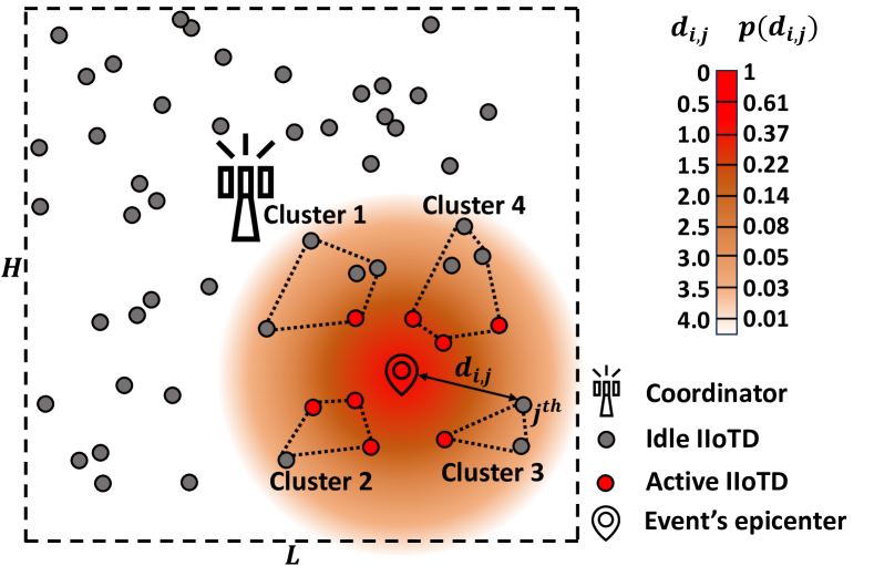
Figure 1: Illustration of an IIoT network where a coordinator controls and collects information from $\displaystyle N=55$ IIoTDs. The influence of an event on the surrounding IIoTDs is modeled by a probability activation function that decays with the distance from the event epicenter to the IIoTDs.

Assume that time is slotted in transmission time intervals (TTIs). The devices report their sensing information in state $\displaystyle A$ (active), while no traffic is generated in state $\displaystyle I$ (idle). We assume that the coordinator knows each IIoTD location and that each event occurs uniformly in the area with probability ($\displaystyle\alpha$) in every TTI [16].

Let us define $\displaystyle p(d_{i,j})$ as a sensing power function that represents the impact of the $\displaystyle i^{\text{th}}$ event, triggered with epicenter $\displaystyle(x_{i},y_{i})$, on the $\displaystyle j^{\text{th}}$ IIoTD within the network area, in the two-dimensional Euclidean plane $\displaystyle\Re^{2}$. Here, $\displaystyle d_{i,j}$ indicates the distance separating them. Moreover, $\displaystyle p(d_{i,j})\rightarrow[0,1]$ is non-increasing to mimic a decaying influence of events as the distance $\displaystyle d_{i,j}$ increases. As an example, Fig. 1 depicts the influence of an event epicenter on the surrounding IIoTDs. Potential functions to be used include exponential [16, 15], linear [17], piece-wise linear [18, 19], and power-law decay [17] for general scenarios, while step [20] or sigmoidal [17] functions may be used for more stringent scenarios like indoor setups. In this paper, we use an exponentially decreasing function, i.e., $\displaystyle p(d_{i,j})=e^{-\eta d_{i,j}}$ [15]. Here, the parameter $\displaystyle\eta$ ($\displaystyle\eta>0$) controls the average sensitivity for a given distance.

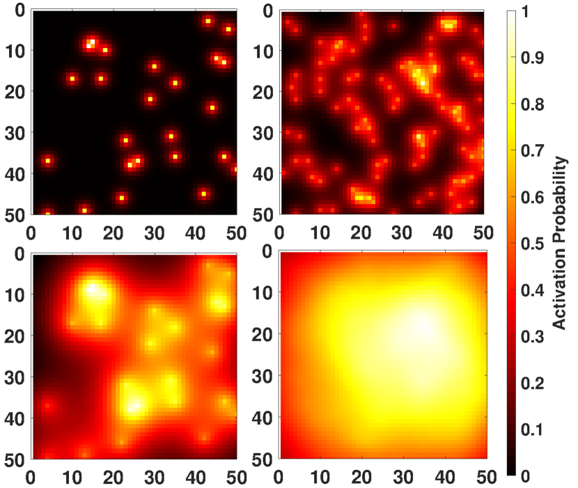
Figure 2: The coverage regions of an illustrative network deployment for a) (top left) $\displaystyle\eta=1$ and 25 IIoTDs, b) (top right) $\displaystyle\eta=1$ and 100 IIoTDs, c) (bottom left) $\displaystyle\eta=0.1$ and 25 IIoTDs, and d) (bottom right) $\displaystyle\eta=0.1$ and 100 IIoTDs. The activation probability shows the event detection coverage.

Note that $\displaystyle\eta$ directly influences network coverage, as depicted in Fig. 2. A high $\displaystyle\eta$ value results in more granulated but smaller coverage, while a smaller $\displaystyle\eta$ value expands the coverage area. Note that the probability of detecting the event is low for the configuration depicted in Fig. 2(a) since there is a large uncovered area. On the other hand, the coverage area in Fig. 2(d) is the most extensive, while in Fig. 2(b-c) the coverage is medium. However, increasing coverage areas comes together with increasing overlapping regions, which is not desired as it leads to increased collision probability and power consumption, contributing to the IIoTDs’ battery depletion. Increasing (decreasing) the activation probability increases (decreases) the power consumption of the IoTDs but also increases the collision (miss-detection) probability in the network. Thus, designing the IIoTDs’ coverage areas for minimum overlap but realizing desired event detection capabilities extends overall coverage and enhances network energy efficiency. In this article, we explore a solution based on IIoTD clustering according to their spatial position/proximity, as depicted in Fig. 1, thus optimizing resource management and enabling localized data processing. In addition, this aids in fault isolation and provides scalability to the IIoT system while improving energy efficiency. Clustering IIoTDs enables the system to quickly detect and isolate faults within a particular cluster, reducing the impact on the overall network. Furthermore, it enhances scalability by managing clusters independently, simplifying the process of adding or removing devices without disrupting the entire system.

III Optimization Problem

In the considered IIoT setup, devices make observations or measurements, which can be used to estimate the probability of successful signal reception, defined here as $\displaystyle p(d_{i,j})$. This probability is typically inferred from historical data or real-time measurements, considering factors such as signal strength and the deployment of IIoTDs. Leveraging sensing signal probabilities, $\displaystyle p(d_{i,j})$, as a guide for transmission decisions holds promise for optimizing network efficiency. This accounts for the likelihood of successful signal reception at various distances, considering interference and IIoTD deployment.

We propose setting (and optimizing) a threshold for each device to decide when to transmit data. We denote $\displaystyle{\delta_{j}}$ as the transmission threshold that is dynamically chosen for the $\displaystyle j^{\text{th}}$ IIoTD. Then, the transmission probability for this $\displaystyle j^{\text{th}}$ IIoTD is given by

$$\Pr\left(A_{j}\right)=\alpha\Pr\left(p(d_{i,j})\geq{\delta_{j}}\right).$$ (1)

Specifically, if the estimated $\displaystyle p(d_{i,j})$ for a given distance is lower than the preset threshold, the device avoids transmission. This is done with the hope that another device has a better observation of the event, thereby avoiding collisions in high-density scenarios, reducing re-transmissions, and conserving energy. This aligns transmission strategies with real-world signal dynamics, promoting more responsive and energy-efficient communication.

Herein, we aim to minimize the energy consumption in the network by optimizing $\displaystyle\boldsymbol{\delta}$$\displaystyle=[\delta_{1},\delta_{2},\dots\delta_{N}]^{\mathbf{T}}$. Specifically, the optimization problem is stated as

$$\displaystyle\text{P}1:\text{ } \displaystyle\min_{{\boldsymbol{\delta}}}\text{ } \displaystyle W(\boldsymbol{\delta})$$ (2a)

s.t. $$\displaystyle\mathbb{E}(P_{\text{e}}(\boldsymbol{\delta})) \displaystyle\leq\text{ }E,$$ (2b)

where $\displaystyle P_{\text{e}}(\boldsymbol{\delta})$ is the error probability given the IIoTDs location and transmission threshold, $\displaystyle\mathbb{E}(P_{\text{e}})$ is its expected value with respect to the events’ epicenters, and $\displaystyle E$ is the imposed error constraint. Meanwhile, $\displaystyle W(\boldsymbol{\delta})$ depicts the expected power consumption per IIoTD in the network, which obeys

$$\begin{array}[]{ll}W({\boldsymbol{\delta}})=\frac{1}{N}\sum_{j=1}^{N}\Pr\left(A_{j}\right).\end{array}$$ (3)

Here, we adopt a simplified energetic model, which is calculated as the proportion of time that the devices are in an active state. We disregard power consumption during idle periods due to its negligible impact on the overall analysis since, in IIoTDs, the primary battery depletion factor comes from radio interface usage. Notice that we assume one transmission window (Tx) per TTI, so more than one IIoTD trying to access the medium at the TTI slot time ($\displaystyle k^{\text{th}}$) is translated into collision.

Collisions occur when multiple devices transmit their shared observations simultaneously, leading to data loss and increasing the expected error probability in our scenario. However, note that failing to detect the presence of an event also increases the error probability. Given an IIoTD deployment, the event error probability $\displaystyle P_{\text{e}}$ captures collision ($\displaystyle P_{\text{col}}$) and miss-detection ($\displaystyle P_{\text{miss}}$) probabilities after the occurrence of an event, i.e.,

$$\begin{array}[]{rl}P_{\text{e}}(\boldsymbol{\delta})=P_{\text{col}}(\boldsymbol{\delta})+P_{\text{miss}}(\boldsymbol{\delta}),\vspace{1mm}\end{array}$$ (4)

since the coordinator does not receive information about this event in both cases. The miss-detection probability is calculated as

$$\begin{array}[]{rl}P_{\text{miss}}(\boldsymbol{\delta})=\alpha\prod_{j=1}^{N}\Pr(p{(d_{i,j})}<{\delta_{j}})\end{array}$$ (5)

due to the event not being detected by any sensor (miss-detection). Conversely, the probability of message notification losses due to collisions when several, more than one IIoTD, transmit at the same time is given by

$$\displaystyle P_{\text{col}}(\boldsymbol{\delta})=\alpha-P_{\text{miss}}(\boldsymbol{\delta})-P_{\text{suc}}(\boldsymbol{\delta}),$$ (6)

where $\displaystyle P_{\text{suc}}$ is the success probability. Therefore, we have that

$$\displaystyle P_{\text{e}}(\boldsymbol{\delta})=\alpha-P_{\text{suc}}(\boldsymbol{\delta}).$$ (7)

Herein, $\displaystyle P_{\text{suc}}$ refers to the union of the detection events from one and only one of the $\displaystyle N$ sensors described as

$$\displaystyle P_{\text{suc}}(\boldsymbol{\delta})=\alpha\sum_{h=1}^{N}\Big{(}\Pr\left(p{(d_{i,j})}\geq{\delta_{h}}\right)\prod_{j\neq h}^{N}\Pr\left(p{(d_{i,j})}<{\delta_{j}}\right)\Big{)}.$$ (8)

Then, the expected value in the network area is given by

$$\mathbb{E}(P_{\text{e}}(\boldsymbol{\delta}))=\alpha-\mathbb{E}(P_{\text{suc}}(\boldsymbol{\delta}))=\int_{\xi}\frac{1}{|\xi|}P_{\text{e}}(\boldsymbol{\delta})\partial\xi.$$ (9)

IV Convex Optimization-based solution

Substituting $\displaystyle\alpha\Pr\textstyle\left(e^{-\eta d_{i,j}}>\delta_{j}\right)$ into (3), the expected power consumption in the network obeys

$$\begin{array}[]{ll}W(\boldsymbol{\delta})=\frac{\alpha}{N}\sum_{j=1}^{N}{\Pr\left(e^{-\eta d_{i,j}}>\delta_{j}\right)}.\end{array}$$ (10)

This is monotonically increasing on $\displaystyle\Pr\left(e^{-\eta d_{i,j}}>\delta_{j}\right)$, which in turn is exponentially decreasing on $\displaystyle\delta_{j}$. Then, the optimization problem can be reformulated as minimizing $\displaystyle\Pr\textstyle\left(e^{-\eta d_{i,j}}>\delta_{j}\right)$ equivalent to $\displaystyle\Pr\left({d_{i,j}}<-\mathrm{ln}(\delta_{j})/\eta\right)$. Note that $\displaystyle d_{i,j}=\textstyle\sqrt{(X-x_{j})^{2}+(Y-y_{j})^{2}}$, where $\displaystyle X$ and $\displaystyle Y$ are random variables. Herein, without losing generality, we assume that $\displaystyle X$ and $\displaystyle Y$ are equally distributed in $\displaystyle[0,L]$ and $\displaystyle[0,H]$, respectively, and $\displaystyle(x_{j},y_{j})$ is the known position of the device $\displaystyle j$.

Theorem 1

Let $\displaystyle Z=d_{i,j}^{2}=(X-x_{j})^{2}+(Y-y_{j})^{2}$, then

$$\displaystyle F_{Z}(z)=\frac{2z}{\xi}\left(\text{arcsin}\left(\sqrt{\frac{u}{z}}\right)+\frac{1}{2}\sin{\left(2\text{arcsin}\left(\sqrt{\frac{u}{z}}\right)\right)}\right),$$ (11)

where $\displaystyle u=\text{max}(x_{j};L-x_{j})^{2}.$

Proof: See proof in Appendix A.

The function in (11) is inherently non-convex and highly non-linear due to the significant oscillations and fluctuations introduced by the trigonometric functions, leading to multiple local minima and maxima. This makes (11) computationally expensive to analyze and optimize. Note however that

$$F_{Z}(z)\approx 1-e^{-\frac{2z}{w}},\text{ for }z\leq 200/\eta^{2},$$ (12)

which is a practical sensing range for low-power IIoTD (less than 5 meters [6], corresponding to $\displaystyle\delta\in[10^{-4},1]$).

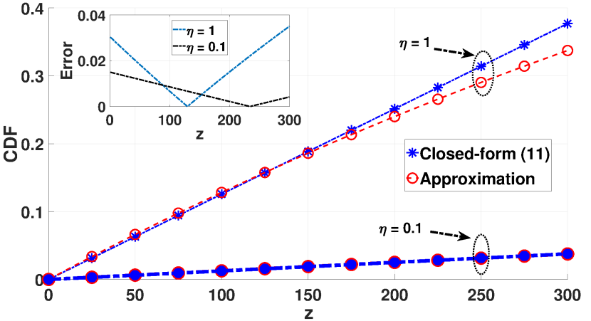
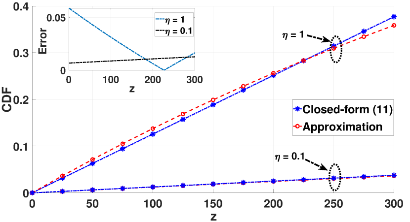
Figure 3: Approximation to (11) fo different $\displaystyle u,v$ and $\displaystyle\eta$ values, (left) $\displaystyle u,v=25$ and (rigth) $\displaystyle u,v=50$.

Fig. 3 illustrates the accuracy of (12) for various values of $\displaystyle u$, $\displaystyle v$, and $\displaystyle\eta$, suggesting its suitability for reformulating the complexity of (2) into a more manageable form. Therefore, $\displaystyle\Pr\left({d_{i,j}}\leq-\mathrm{ln}(\delta_{j})/\eta\right)$ can be reformulated as $\displaystyle\Pr\left({z_{j}}\leq\mathrm{ln^{2}}(\delta_{j})/\eta^{2}\right)=F_{z}\left(\mathrm{ln^{2}}(\delta_{j})/\eta^{2}\right)$, which is monotonically increasing, and P1 can be rewritten as

$$\displaystyle\text{P}2:\text{ } \displaystyle\min_{\boldsymbol{\delta}}\text{ } \displaystyle\sum_{j=1}^{N}{F_{z}\left(\mathrm{ln^{2}}(\delta_{j})/\eta^{2}\right)}$$ (13a)

s.t. $$\displaystyle\mathbb{E}(P_{\text{e}}(\boldsymbol{\delta}))\leq\text{ }E.$$ (13b)

Herein, $\displaystyle\mathbb{E}(P_{\text{e}}(\boldsymbol{\delta}))$ can be computed by substituting (8) into (9), wherein

$$\displaystyle\mathbb{E}(P_{\text{suc}}(\boldsymbol{\delta}))= \displaystyle\alpha\sum_{h=1}^{N}\left(1-e^{-\frac{2\mathrm{ln^{2}}(\delta_{h})}{w_{h}}}\right)\prod_{j\neq h}^{N}e^{-\frac{2\mathrm{ln^{2}}(\delta_{j})}{w_{j}}}$$

$$\displaystyle= \displaystyle\alpha\sum_{h=1}^{N}\left(1-e^{-\frac{2\mathrm{ln^{2}}(\delta_{h})}{w_{h}}}\right)e^{-2\sum_{j\neq h}^{N}\frac{\ln^{2}\delta_{j}}{w_{j}}}$$

$$\displaystyle= \displaystyle\alpha\sum_{h=1}^{N}e^{-2\sum_{j\neq h}^{N}\frac{\ln^{2}\delta_{j}}{w_{j}}}+{\alpha}{N}e^{-2\sum_{j=1}^{N}\frac{\ln^{2}\delta_{j}}{w_{j}}}.$$ (14)

Hence,

$$\displaystyle\mathbb{E}(P_{\text{e}}(\boldsymbol{\delta}))= \displaystyle\alpha-\alpha\sum_{h=1}^{N}e^{-2\sum_{j\neq h}^{N}\frac{\ln^{2}\delta_{j}}{w_{j}}}+{\alpha}{N}e^{-2\sum_{j=1}^{N}\frac{\ln^{2}\delta_{j}}{w_{j}}}.$$ (15)

However, solving this optimization problem is still non-trivial since the objective and constraint functions are not convex (see proof in Appendix B).

Convex optimization techniques have been promising in addressing various challenges in wireless communication systems, including optimizing beamforming for enhanced signal transmission [21], power consumption minimization [22], and refining device localization methods for precise positioning [23]. Moreover, interior point methods (IPM) [24, 25], which are known to converge in/with polynomial time/complexity, are commonly utilized for solving convex problems [26, 27]. In the following subsections, we will discuss the fundamental principles of convex approximation methods used in this paper and how they address P2. Such an optimization problem can be solved by iterative approximation methods like SCA [28, 25] or BCD [29], where an inner convex approximation in each iteration approximates the non-convex feasible set. By using the approximation methods, an approximate solution to the optimization problem in (13) can be attained using standard convex optimization tools such as CVX [28] or fmincon of MATLAB [30].

IV-A Successive Convex Approximation (SCA)

Algorithm 1 SCA

1:Initialization: Choose initial $\displaystyle\boldsymbol{\delta_{0}}$

2:for $\displaystyle k=0,1,2,\ldots,g-1$ do

3:    Solve the surrogate problem using $\displaystyle\mathcal{T}(\cdot)$ around $\displaystyle\boldsymbol{\delta}_{k}$ such that $\displaystyle{\boldsymbol{\hat{\delta}}}_{k}=\arg\min_{\boldsymbol{\delta}}W(\boldsymbol{\delta})\text{ }\text{s.t. }\mathbb{E}(P_{\text{e}}(\boldsymbol{\delta}))\leq E$

4:    Update with learning rate $\displaystyle\vartheta_{k}:\boldsymbol{\delta}_{k+1}=\boldsymbol{\delta}_{k}+\vartheta_{k}\left({\boldsymbol{\hat{\delta}}}_{k}-\boldsymbol{\delta}_{k}\right)$

5:end for

6:Return $\displaystyle\boldsymbol{\delta}_{k}$

To solve P2 using SCA, we approximate the constraint function with its first-order Taylor series and iteratively optimize the objective function. Also, we use regularization to enforce convergence. Herein, we define $\displaystyle\mathcal{T}(\cdot)$ as the operator approximating an input function using its first-order Taylor series expansion. The first-order Taylor series approximation is used to estimate the constraint around $\displaystyle\boldsymbol{\delta_{0}}$. This constraint is a vector of initial values of $\displaystyle\boldsymbol{\delta}$ that gets updated in each SCA iteration by the resulting value obtained in the previous iteration. The error probability and its first derivative is evaluated in $\displaystyle\boldsymbol{\delta}$, Thus, it is given by

$$\displaystyle\mathcal{T}(\mathbb{E}(P_{\text{e}}(\boldsymbol{\delta})))= \displaystyle\mathbb{E}(P_{\text{e}}(\boldsymbol{\delta_{0}}))+(\boldsymbol{\delta}-\boldsymbol{\delta_{0}})^{\mathbf{T}}\nabla\mathbb{E}(P_{\text{e}}(\boldsymbol{\delta_{0}})),$$ (16)

where

$$\displaystyle\!\nabla_{\delta_{j}}\mathbb{E}(P_{\text{e}}(\boldsymbol{\delta}))\! \displaystyle=\!\frac{4\alpha\mathrm{ln}(\delta_{j})}{w_{j}\delta_{j}}\!\left(\sum_{h=1}^{N-1}\!e^{-2\sum_{i\neq h}^{N}\!\frac{\ln^{2}\delta_{i}}{w_{i}}}\!\!-\!e^{-2\sum_{i=1}^{N}\!\frac{\ln^{2}\delta_{i}}{w_{i}}}\!\!\right).$$ (17)

Algorithm 1 depicts the SCA algorithm for each iteration $\displaystyle k$. Note that the complexity when implementing SCA is $\displaystyle\mathcal{O}(gf({\boldsymbol{\delta}}))$, where $\displaystyle g$ is the maximum number of iterations.

IV-B Block coordinate descending method (BCD)

Algorithm 2 BCD

1:Initialization: Choose initial $\displaystyle\boldsymbol{\delta_{0}}$

2:for $\displaystyle k=0,1,2,\ldots,g-1$ do

3:    for $\displaystyle j=1,2,\ldots,N$ do

4:         Solve P2 for variable $\displaystyle{{\hat{\delta_{j}}}}$ with $\displaystyle\delta_{h\neq j}$ fixed, i.e., $\displaystyle{{{\hat{\delta_{j}}}}=\arg\min_{\delta_{j}}}\text{ }W(\boldsymbol{\delta})\text{ }\text{s.t. }\mathbb{E}(P_{\text{e}}(\boldsymbol{\delta}))\leq E$

5:    end for

6:    $\displaystyle\boldsymbol{\delta}_{k+1}={\boldsymbol{\hat{\delta}}}_{k}$

7:end for

8:Return $\displaystyle\boldsymbol{\delta_{k}}$

In the conventional BCD framework, the formulated non-convex sparse recovery problem can be decomposed into small-scale sub-problems after exploiting the least absolute shrinkage and selection operator-based regularization [29]. Subsequently, the variables in each sub-problem can be optimized sequentially with variables from other sub-problems kept fixed. Herein, we also approximate the constraint function with its first-order Taylor series, as in SCA, but in this case, the function has just one variable in each iteration, while the rest are fixed. The method runs $\displaystyle N$ iterations in which the problem is solved for one variable at each step, fixing the rest of $\displaystyle(N-1)$ variables, running $\displaystyle N$ sequential problems with one variable in an inner loop, and repeating the method $\displaystyle g$ times (maximum iteration). Algorithm 2 summarizes BCD algorithm and note that its complexity is $\displaystyle\mathcal{O}(gNf({\boldsymbol{\delta}}))$.

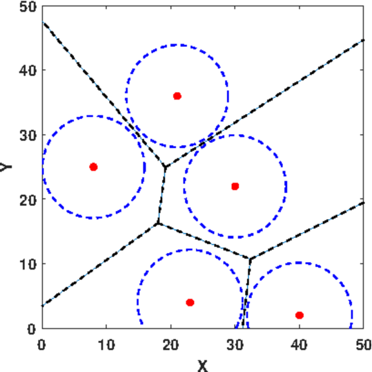
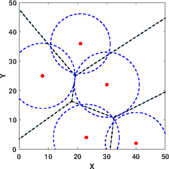
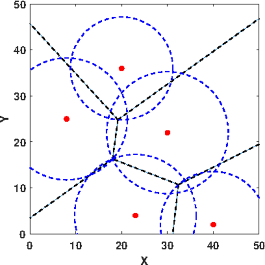
Figure 4: Illustration of a Voronoi diagram for a grid IIoT deployment with 5 devices (represented as red dots). The black lines represent the Voronoi polygon corresponding to each IIoTD, while the blue lines represent the sensing area border. (left) Voronoi-(i), (center) Voronoi-(ii), and (right) Voronoi-(iii).

V Heuristic & Data-driven proposed solutions

Relying on previous optimization techniques can be computationally expensive and time-consuming, especially for large-scale IoT systems. Herein, we aim to explore heuristic and data-driven approaches to efficiently solve the problem. Note that heuristic approaches may lead to near-optimal solutions relatively quickly. In contrast, data-driven solutions can learn from the available data and make predictions based on the learned patterns. Metaheuristic methods such as GA [31] and PSO [32] are valid tools, along with online methods like RL [33] and Lyapunov optimization [34], which also offer adaptability.

In the following, we present potential approaches to solve the problem. The first two solutions are heuristics, one based on the Voronoi diagram and the other on clustering and Bayes’ theorem, specifically KNN. The third solution uses metaheuristic numerical methods and requires GA and PSO tools. The fourth and final approach is a RL-based solution. Notice that, unlike the metaheuristic methods, such heuristic learning can be performed online, as it does not require an oracle view of the network for re-training. Specifically, the sensors can independently implement and change strategies in case of re-training, using acknowledgments for correctly transmitted packets as their only feedback while knowing the position of the sensors (fixed) in its cluster and their threshold.

V-A Voronoi-based approach

Herein, we optimize $\displaystyle\boldsymbol{\delta}$ using the Voronoi graph theory applied to the IIoT deployment. The principle of the Voronoi diagram has been maturely applied to computer graphics research, occupying an important role in computational geometry [35]. A Voronoi diagram comprises a set of continuous polygons formed by vertical bisectors connecting two neighboring edges [36]. The bisector is the trajectory of all points at equal distances to neighboring IIoTD. A Voronoi diagram has three basic properties: (i) each Voronoi area is unique; (ii) the adjacent Voronoi area of each Voronoi area is the nearest adjacent area in the Euclidean plane; and (iii) each Voronoi area has at least three edges, and the edges are closed [36]. Fig. 4 depicts a simplified and easily interpretable Voronoi diagram of an IIoT deployment with 5 devices.

The Voronoi diagram’s definition and unique properties can be harnessed to partition areas and employ the resulting polygons for each device as a metric for optimizing transmission thresholds. Specifically, we use the polygon metrics to calculate the optimal $\displaystyle\delta_{j}=e^{-\eta\Omega_{j}}$, where $\displaystyle\Omega_{j}$ (blue lines in Fig. 4) represents the target coverage radio per IoTD, and it is obtained by using three approaches as follows

• minimum distance from the IIoTD to its polygon;

• mean distance from the IIoTD to its polygon;

• maximum distance from the IIoTD to its polygon.

When employing a Voronoi-based approach, the worst-case complexity is $\displaystyle\mathcal{O}(2N\log N)$ [37].

V-B Bayesian-based KNN

Recently, ML capabilities and utilization have tremendously increased in various fields. While cutting-edge ML models provide invaluable benefits, they often function as black boxes, which makes it difficult for humans to understand their decision-making processes. Indeed, complex models such as deep neural networks have multiple parameters and intricate structures to the point of being considered black boxes with low understandability.

The demand for transparency has prompted the emergence of Explainable AI (XAI). XAI is a field dedicated to developing AI methods that serve two primary objectives: i) to generate more comprehensible models while ensuring their learning efficiency remains high and ii) to enable humans to trust, understand, and effectively manage these AI systems. Note, for instance, that ML models such as linear/logistic regression, decision trees, KNN, rule-based learners, general additive models, and Bayesian models are more easily understood and manipulated by humans. These models are transparent by design and have a greater explaining capacity than complex models like deep neural networks, as depicted in Fig. 5, inspired in [38].

Herein, we adopt KNN [39, 40] and Bayesian Models [41], widely used XAI approaches in the IIoT context because of their trade-off accuracy/interpretability and simplicity.

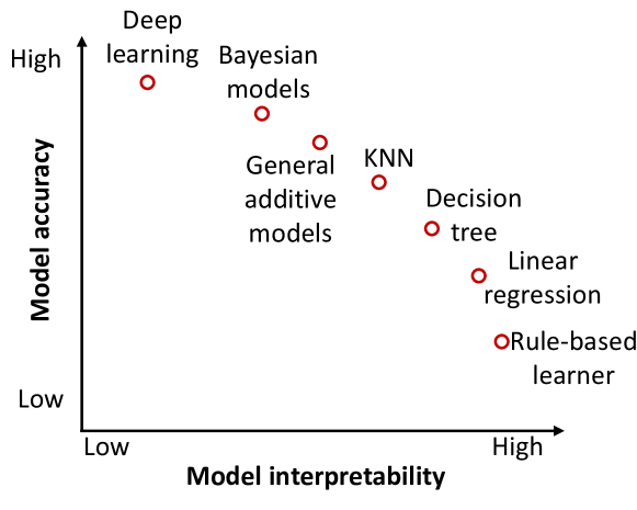
Figure 5: The trade-off between model interpretability and performance.

Specifically, we propose a heuristic approach wherein we form clusters based on each device’s spatial placement using KNN, thus each data point is connected to its K-nearest neighbors, creating a graph structure. Note that the considered IIoT network is stationary, i.e., devices’ positions are fixed and known, thus the computational cost associated with implementing KNN is $\displaystyle\mathcal{O}(N(N-1)/2)$ in the worst-case scenario (brute force). This complexity arises due to the need to calculate distances to the $\displaystyle N$ IIoTD for each query point. The search involves scanning the entire dataset to identify the KNN. However, as previously mentioned, the computation time can differ based on the utilized algorithm, occasionally reducing to $\displaystyle\mathcal{O}(\min\{M(N-M),(N-M)^{2}\})$, where $\displaystyle M$ is the number of clusters [37]. Note that we only form clusters once for a given IIoTD deployment, thus it can be implemented offline.

After establishing the clusters, as depicted in Fig. 6 (see also Fig. 1) as an example, we employ a greedy conditional probability rule, the generalized Bayes’ rule. We start from the edges that statistically require a larger sensing area, i.e., a lower threshold, to cover the entire area effectively and prevent miss-detection. Each device constitutes the center of a cluster according to the spatial correlation to its nearest neighbors, forming a graph structure. Initially, the devices’ activation probability is set randomly. Then, we begin by updating the transmission threshold for each device by taking into account its spatial correlation with its nearest neighbors. We calculate $\displaystyle\delta_{j}$ based on the transmission thresholds of the neighbors and its transmission threshold, taking into account the spatial correlation as well. Then,

$$\Pr\left(p(d_{i,j})\geq{\delta_{j}}\right)=\sum_{\forall h}\Pr(A_{j}|A_{h})\Pr\left(p(d_{i,h})\geq{\delta_{h}}\right),$$ (18)

where $\displaystyle\Pr(A_{j}|A_{h})$ is the conditional probability for the device $\displaystyle j$ being active given that device $\displaystyle h$ is active.

Theorem 2

Let $\displaystyle R=\min(x_{h},y_{h},H-x_{h},L-y_{h})$ and $\displaystyle r=\max(R,d_{h})$, then

$$\displaystyle\Pr(A_{j}|A_{h})=1-\frac{\cos^{-1}\left(\frac{d_{i,h}^{2}+r^{2}_{j,h}-\mathrm{ln^{2}}(\delta_{j})/\eta^{2}}{2d_{i,j}r_{j,h}}\right)}{2\pi-8\cos^{-1}\left(R/r\right)},$$ (19)

where $\displaystyle r_{j,h}$ is the distance between the IIoTDs $\displaystyle j$ and $\displaystyle h$, and $\displaystyle\varphi$ represents the angle at the event epicenter determined by the IIoTDs $\displaystyle j$ and $\displaystyle h$ positions.

Proof: See proof in Appendix C.

Finally, the complexity when implementing the Bayesian-based KNN algorithm is bounded by $\displaystyle\mathcal{O}(gN+\min\{M(N-M),(N-M)^{2}\})$, where $\displaystyle g$ is the maximum number of iterations to converge. Note that the required iterations vary depending on the initial value for $\displaystyle\boldsymbol{\delta}$.

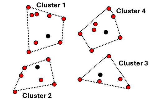
Figure 6: Illustration of an IIoT deployment clustering with 30 IIoTDs and 4 clusters. The dot lines represent the cluster edges and the black dots represent IIoTDs acting as cluster heads.

V-C Genetic algorithm (GA)

We employ a GA for its capacity to explore extensive solution spaces and tackle nonlinear, non-convex problems efficiently. GAs are well-suited for parallelization and scalability [42] and adapt to dynamic and changing environments. Unlike black-box approaches, GAs provide flexibility and adaptability while maintaining transparency [43, 44]. These meta-heuristic algorithms inspired by biological evolution are straightforward to construct and demand relatively modest storage.

GAs systematically explore the state space and iteratively apply mutation, crossover, and selection operations [31]. Specifically, an initial population of size $\displaystyle\Theta$ with potential solutions is generated first. Different $\displaystyle\boldsymbol{\delta}$ initialization are generated with random threshold values. Note that increasing the population size increases the probability of finding a near-optimal solution, but the execution complexity also increases. The best-fit potential solutions are probabilistically selected from the current population based on the objective and constraint functions of (13). Then, the threshold parameters for each device undergo modifications, including recombination and potential random mutations, to generate a new generation [31]. Crossover combines activation probabilities of devices from different parent solutions, while mutation introduces random changes in these probabilities to promote exploration. The algorithm works by repeatedly going through a process of evolution, where the population changes over time and individuals are adjusted based on their fitness until an optimal or near-optimal solution is found. This process continues until either the optimization objective is met or the maximum number of iterations is reached (as defined by the parameter $\displaystyle g$).

Using this meta-heuristic algorithm, we approximate a near-optimal configuration with a complexity of $\displaystyle\mathcal{O}(g\beta)$, where $\displaystyle g$ is the maximum number of iterations, and $\displaystyle\beta$ represents the cardinality of the candidate population vector, which depends on the parameter values $\displaystyle N$ and $\displaystyle\Theta$ as follows, $\displaystyle\beta=N\Theta$. Parameter fitness is assessed in each generation using the objective and constraint functions in (13).

V-D Particle swarm optimization (PSO)

PSO is exceptional in dynamic and nonlinear spaces with a high complexity degree [32] and thus it is a compelling choice for addressing P2. PSO operates on the principles of swarm intelligence, mirroring the collaborative behavior of particles in nature. This is appealing in IIoT systems, where numerous devices must work together efficiently [32, 45].

Like in GA, a population $\displaystyle\Theta$ of threshold sets is randomly initialized within the threshold space $\displaystyle(0,1]$, where each threshold set represents a potential solution. Then, we evaluate the potential solutions using (13) and based on the optimization goal. In each iteration, the threshold sets adjust their activation probabilities based on knowledge of better individual and global solutions discovered by themselves and the swarm. Specifically, we determine $\displaystyle{\delta_{j}}$ for each device by using a fixed value for the other devices’ thresholds and selecting the best potential solutions in the population. At each iteration, we assess the fitness of each particle’s solution using (13), then update the individual $\displaystyle{\delta_{j}}$ and global best $\displaystyle\boldsymbol{\delta}$ based on any improvements in fitness. This allows us to refine and improve the overall solution. PSO continues iterations until an optimal or near-optimal solution that satisfies the optimization objective is found, or the number of iterations parameter ($\displaystyle g$) reaches the preset maximum number. The best global solution found represents optimized activation probabilities. Herein, we approximate a near-optimal configuration using PSO with a complexity of $\displaystyle\mathcal{O}(gN\Theta)$. Note that the population of potential solutions can be initialized based on the spatial correlation relation from heuristics like Voronoi, which may decrease the complexity to reach a near-optimal solution.

V-E Reinforcement Learning (RL)

Model-free RL is a programming tool to tackle decision-making challenges and learn optimal solutions in dynamic environments [46]. Herein, we reframe the optimization problem by introducing spatially-based transmission thresholds and approach it as RL challenge. The IIoT system is conceptualized as the environment, while the devices function as learning agents in this setup. A coordinator retains decision-making authority to prevent computational overload at the IIoTDs, representing them virtually. The central controller stationed at the coordinator provides notifications for miss-detection and collisions. The fundamental components of RL are described as follows.

Let $\displaystyle\mathcal{S}$ denote the system state space. The current system state $\displaystyle s\in\mathcal{S}$ includes the state of each device (active or inactive) and their received sensing power from the event, depicted by the sensing function $\displaystyle p(d_{i,j})$. Consequently, it also includes information corresponding to collisions and miss-detections. In addition, the known position of the devices and their current thresholds are also known. The current state of each device is defined as

$$\begin{array}[]{rl}s=\{\{\delta_{j}\}_{\forall j\in\mathcal{J}},\{p(d_{i,j})\}_{\forall j\in\mathcal{J}},\{(x_{j},y_{j})\}_{\forall j\in\mathcal{J}}\}.\end{array}$$ (20)

With an observed state ‘$\displaystyle s$’ given, the coordinator varies $\displaystyle\delta$ for each device according to the reward/penalty function. The action space is then delimited by threshold limits as $\displaystyle\delta_{j}\in(0;1];$ $\displaystyle\forall j\in\mathcal{J}$. The reward must capture the effectiveness of the threshold policy when the agent takes an action in the current state. In each learning step, the system’s performance must align with the reward function [46], enhancing energy efficiency while avoiding errors. This reward function represents our optimization goal, which is to maximize the system’s overall energy efficiency. Therefore, the reward function at a TTI $\displaystyle\tau$ is expressed as

$$\displaystyle\!r_{\tau}\!=\!\!\!\!\sum_{j,h\in\mathcal{J}}\!\!\!\Pr(A_{j}|A_{h})\!\Pr\!\left(p(d_{i,j})\!\!\geq\!\!{\delta_{h}}\right)\!-\!\mu_{1}p(d_{i,j})\rho_{j}\!-\!\mu_{2}p(d_{i,j})\sigma\!,$$ (21)

where the coefficients $\displaystyle\mu_{1}$ and $\displaystyle\mu_{2}$ are the positive constants used to balance the utility and cost. Additionally, $\displaystyle\Pr(A_{j}|A_{h})$ accounts for the conditional activation probability between IIoTD in position ($\displaystyle x_{j},y_{j}$) given an active IIoTD in ($\displaystyle x_{h},y_{h}$). On the other hand, the second and last terms are penalized to account for situations that provoke error. Specifically, $\displaystyle\rho_{j}$ accounts for the collision effect factor given by

$$\begin{array}[]{rl}\rho_{j}&=\begin{cases}1,&\text{if collision occurs and}\Pr\left(p(d_{i,j})\geq{\delta_{j}}\right),\\ \hfil-1,&\text{otherwise.}\\ \end{cases}\\ \end{array}$$ (22)

Moreover, $\displaystyle\sigma$ is the miss-detection factor given by

$$\begin{array}[]{rl}\sigma&=\begin{cases}1,&\text{if no IIoTD is active,}\\ \hfil 0,&\text{otherwise.}\\ \end{cases}\\ \end{array}$$ (23)

Herein, we assume that the coordinator detects event miss-detection during training. Note that $\displaystyle\rho_{j}$ and $\displaystyle\sigma$ impose the error probability satisfaction level. If no collision or miss-detection occurs, then $\displaystyle\rho_{j}=0$ or $\displaystyle\sigma=0$, indicating no penalization to the reward function due to any error. The idea is finding an optimal policy $\displaystyle\pi^{*}$ at each state $\displaystyle\tau$ (mapping states in $\displaystyle\mathcal{S}$ to the probability of choosing an action $\displaystyle{\pi_{j}^{*}(s)\in[-\delta_{j}^{*},1-\delta_{j}^{*}]}$, with $\displaystyle{s_{\tau}+\pi^{*}\rightarrow s_{\tau+1}}$) [33] that maximizes the long-term expected discounted reward. The cumulative discounted reward is given by

$$\begin{array}[]{rl}U_{\tau}=\sum_{k=0}^{\tau}\zeta^{k}r_{k+1},\end{array}$$ (24)

where $\displaystyle\zeta\in(0,1]$ is the discount factor that grows exponentially with each state $\displaystyle\tau$ and $\displaystyle r_{\tau+1}$ is the reward at the next state.

Moreover, the state-action function of the agent with a state-action pair $\displaystyle(s,a)$ under a policy $\displaystyle\pi$ is given by

$$\begin{array}[]{rl}Q^{\pi}_{\tau}(s_{\tau},a_{\tau})=\mathbb{E}_{\pi}[U_{\tau}|s=s_{\tau},a=a_{\tau}],\end{array}$$ (25)

where a conventional Q-learning algorithm can be adapted to learn the optimal policy by updating the Q-table using Bellman’s equation to reach the optimal action-value function [47]. Furthermore, the Q-value is updated as follows

$$\displaystyle Q_{\tau+1}^{\pi}(s_{\tau},a_{\tau}) \displaystyle=(1-\omega_{\tau})Q_{\tau}^{\pi}(s_{\tau},a_{\tau})+\dots$$

$$\displaystyle+\omega_{\tau}(r_{\tau}+\zeta_{\tau}\max_{a_{\tau}}Q^{\pi^{*}}(s_{\tau+1},a_{\tau+1})),$$ (26)

where $\displaystyle\omega_{\tau}\in(0,1]$ is the learning rate.

$\displaystyle Q$-Learning generally constructs a lookup $\displaystyle Q$-table $\displaystyle Q(s,a)$, and the agent selects actions based on an $\displaystyle\epsilon$-greedy policy for each learning step [48]. In the $\displaystyle\epsilon$-greedy policy, the agent chooses the action with the maximum $\displaystyle Q$-table value with probability $\displaystyle(1-\epsilon)$, whereas a random action is picked with probability $\displaystyle\epsilon$ to support exploration and avoid getting stuck at non-optimal policies [46]. Once the optimal $\displaystyle Q$-function $\displaystyle Q^{*}(s,a)$ is achieved, the optimal policy is determined by

$$\begin{array}[]{rl}\pi^{*}(s,a)=\arg\max_{a_{\tau}}Q^{*}(s,a).\end{array}$$ (27)

The complexity of the RL-based approach might vary depending on the initial values and the algorithm implementation. However, the worst-case algorithm complexity is $\displaystyle\mathcal{O}(N^{2})$.

VI Complexity Analysis

Herein, we summarize and discuss the complexity of the proposed optimization algorithms. We compare our proposals with a conventional implementation where each device has the same threshold (sensitivity) configured [16], i.e., $\displaystyle\delta_{j}=\delta$, $\displaystyle\forall j\in\mathcal{J}$. Notice that the problem in (13) is easily solved for an equal activation threshold since the sum and multiplication of probabilities in the objective and constraint function become an arithmetic and geometric mean with only one variable (see Appendix D).

The complexity for equal-$\displaystyle{\delta}$, SCA, and BCD depends on the complexity of performing IPM to solve $\displaystyle f({\boldsymbol{\delta}})$ [49], which depends on the inequality constraints and the complexity of a typically polynomial method. In this case, there is just one inequality constraint and the worst-case complexity to solve the problem using IPM is $\displaystyle\mathcal{O}(N^{3})$ and typically converges for $\displaystyle g=\sqrt{N}$ iterations. Note that this value varies depending on the suitability of the initial values. Here, for equal-$\displaystyle{\delta}$ and BCD, the problem is evaluated in a summation of $\displaystyle N$ terms with one variable, thus the complexity is $\displaystyle\mathcal{O}(N^{3})$ for equal $\displaystyle{\boldsymbol{\delta}}$ while for BCD is $\displaystyle\mathcal{O}(N^{9/2})$ since the problem is solved $\displaystyle N$ times and converges in $\displaystyle\sqrt{N}$. Meanwhile, the complexity for SCA is $\displaystyle\mathcal{O}(N^{7/2})$ since there is a summation of $\displaystyle N$ terms with a vector $\displaystyle{\boldsymbol{\delta}}$ of $\displaystyle N$ variables. Without losing generality, we assume that the complexity of evaluating a variable is $\displaystyle\mathcal{O}(1)$.

Table II summarizes the methods’ complexity. We can see that the equal-$\displaystyle{\delta}$ and Voronoi approaches do not depend on the iterations to converge, while the rest do. However, the rest depends on the specific algorithms and how fast they converge. Moreover, the computational complexity of implementing the proposed methods exhibits polynomial behavior. BCD is the most complex method, while Voronoi and KNN are comparatively less complex. Additionally, although RL is the most energy-efficient method, it is the only one that requires online implementation or a quite wide dataset. It is noteworthy that when implementing RL with an initial $\displaystyle\boldsymbol{\delta}$ based on previous algorithm results like SCA or Voronoi, rather than random $\displaystyle\boldsymbol{\delta}$ initialization, the complexity decreases up to $\displaystyle\mathcal{O}(N\log N)$. Therefore, RL could be implemented either offline with a history dataset or to retrain the system in a dynamic scenario.

TABLE II: Complexity analysis

Algorithm	Complexity
Equal $\displaystyle\boldsymbol{\delta}$	$\displaystyle\mathcal{O}(N^{3})$
SCA	$\displaystyle\mathcal{O}(N^{3}\sqrt{N})$
BCD	$\displaystyle\mathcal{O}(N^{4}\sqrt{N})$
Voronoi	$\displaystyle\mathcal{O}(N\log N)$
Bayesian-based KNN	$\displaystyle\mathcal{O}(gN+(N-M)(\min\{M,N-M\}))$
GA	$\displaystyle\mathcal{O}(gN\Theta)$*
PSO	$\displaystyle\mathcal{O}(gN\Theta)$
RL	$\displaystyle\mathcal{O}(N^{2})$

*Note that good choices for $\displaystyle g$ and $\displaystyle\Theta$ may increase with $\displaystyle N$.

VII Results

Consider a 50$\displaystyle\times$50 m² area with $\displaystyle N\in[25\text{ }250]$ devices. We choose $\displaystyle N\geq 25$ since for smaller numbers the optimization problem often becomes unfeasible as there are not enough devices to cover the area. Indeed, miss-detection events are very common for $\displaystyle N<25$. Additionally, we consider $\displaystyle\alpha=0.1$, $\displaystyle{\eta=1}$ [15], and set $\displaystyle E=0.1$ and $\displaystyle g=\sqrt{N}$. We perform 250 Monte Carlo runs corresponding to different deployments. For simplicity, the power consumption is given without units (percentage of time in active state). However, the value can be obtained by multiplying this value and the power consumption of the specific device in an active state.

VII-A Benchmark and Voronoi approaches

We adopt the equal-$\displaystyle{\delta}$ approach as a benchmark. Initially, we assess the power consumption linked to employing the equal-$\displaystyle{\delta}$ approach and compare it with the four Voronoi-based solutions. It’s noteworthy that the optimization problem might not always be solvable with the equal-$\displaystyle{\delta}$ approach and the latter three Voronoi-based alternatives, due to non-compliance with the error constraints.

In Fig. 7, we show the mean energy consumption per device in the network when using the two previous solutions. Note that the Voronoi-(i) algorithm has the best performance, while the scenario with equal-$\displaystyle{\delta}$ and Voronoi-(iii) has the worst performance related to energy consumption. Herein, note that equal-$\displaystyle{\delta}$ slightly outperforms Voronoi-(iii) for more than 33 IIoTDs. Indeed, the sensing area in the latter approach is determined by the biggest distance to the Voronoi polygon, hence, the overlapping probability in sensing areas for neighbor IIoTD is high and the energy efficiency low. However, Voronoi-(i) is the only algorithm capable of finding a solution to the optimization problem in each scenario. The other approaches can find solutions in just some cases, as depicted in Fig. 8. In this case, both approaches with the worst performance can find a solution between 49% (equal-$\displaystyle{\delta}$) to 55% (Voronoi-(iii)) of the time, while the feasibility is about 72%-74% for Voronoi-(ii).

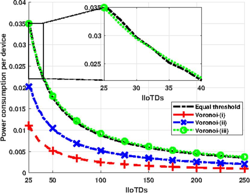
Figure 7: Power consumption as a function of the number of IIoTDs for the benchmark and the Voronoi approaches.

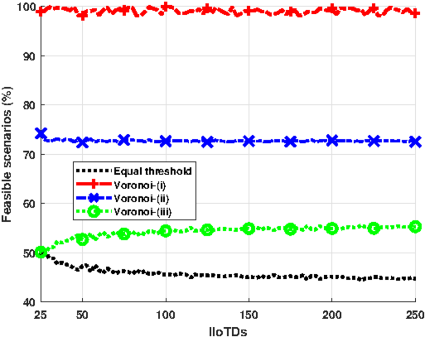
Figure 8: Feasibility rate to find a configuration with $\displaystyle P_{e}\leq 0.1$ as a function of the number of IIoTDs for the benchmark and Voronoi’s approaches.

Based on the above discussions, only the Voronoi-(i) approach is adopted for comparison purposes in the following. It is worth noting that the equal-$\displaystyle{\delta}$ solution, although not always feasible according to the constraint, will still be included in the comparisons for benchmarking purposes.

VII-B Performance comparison

Herein, we present performance results for the proposed energy-efficient solutions. Notably, these solutions are feasible across all 250 modeled scenarios, unlike the benchmark and Voronoi’s approaches analyzed in Section VII-A. Specifically, Fig. 9 shows the power consumption per device as a function of the device density and using the approximation methods. Herein, BCD and RL have the worst and best performance, respectively. Interestingly, as we increase the device density, SCA and KNN show a performance similar to RL. Meanwhile, GA and PSO show similar performances and outperform the equal-$\displaystyle{\delta}$ approach. On the other hand, BCD outperforms the equal threshold scheme for a density below 150 IIoTDs. However, it consumes more power when the density increases above 150. Notice that for the equal-$\displaystyle{\delta}$ scenario, the error probability constraints can not be met for around half of the scenarios modeled. Here, the RL approach reduces the power consumption by up to 96% compared with the benchmark for low-density scenarios, while for high-density scenarios, the consumption is reduced by 60%. As expected, the power consumption decreases as IIoTDs density increases because coverage increases, allowing for a smaller sensing area to be set for each IIoTD, thereby lowering their activation probability for most approaches.

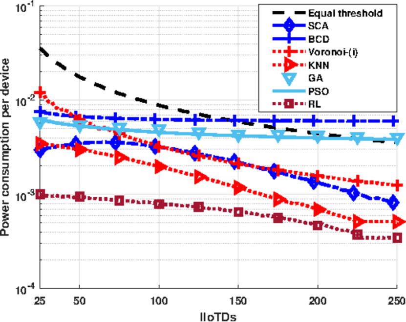
Figure 9: Power consumption as a function of the number of IIoTDs per device for the proposed solutions.

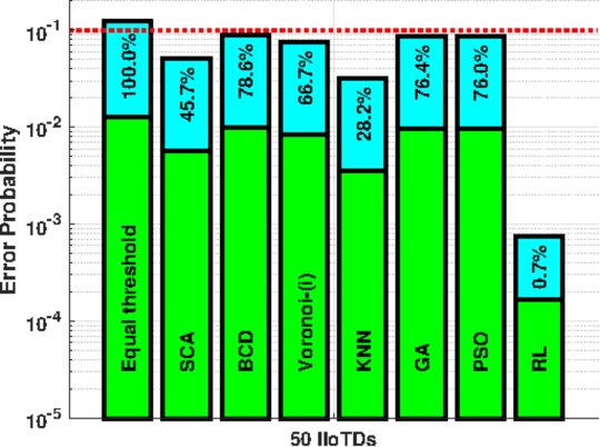
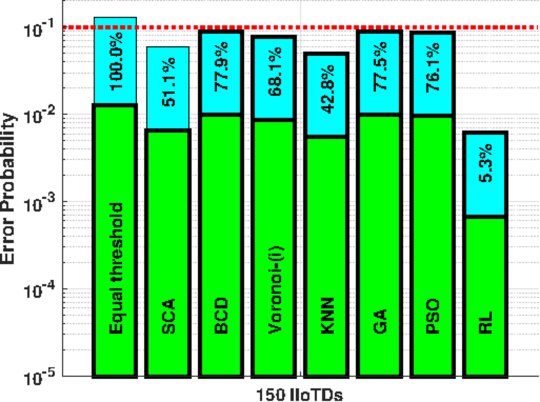
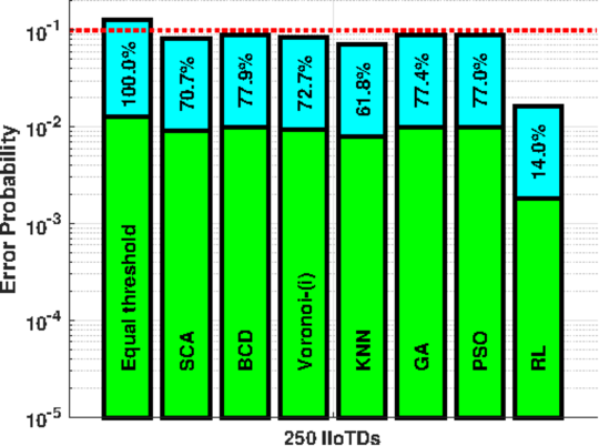
Figure 10: Error probability ($\displaystyle P_{\text{e}}$) for the proposed solutions as the sum of the collision (cyan) and miss-detection (green) probabilities for (left) 50, (center) 150, and (right) 250 IIoTDs. The percentages indicate the error probability of the methods compared to the equal-$\displaystyle\delta$ approach, while the red dotted line represents the error constraint $\displaystyle E$.

In addition, Fig. 10 displays $\displaystyle P_{\text{e}}$ for the proposed methods, which combines the collision (cyan) and miss-detection (green) probabilities. It’s worth noting that $\displaystyle P_{\text{e}}$ is consistently below 0.1 for each of the proposed solutions, meeting the constraint $\displaystyle E$ in P2, while the equal-$\displaystyle\delta$ approach fails to stay below this limit. The value of $\displaystyle P_{\text{miss}}$ remains almost constant, staying below 0.01. It’s important to highlight that the RL approach demonstrates the lowest $\displaystyle P_{\text{e}}$, whereas BCD, GA, and PSO exhibit the highest values. Notably, the value of $\displaystyle P_{\text{e}}$ increases with higher IIoTD density, as more devices are likely to collide upon activation from the same event. Furthermore, Fig. 10 also illustrates the relative error probability of the proposed methods compared to the equal-$\displaystyle\delta$ approach. Notably, in low-density scenarios, SCA, KNN, and RL reduce the error probability by up to 45.7%, 28.2%, and 0.7% respectively. However, in high-density scenarios, only RL is capable of reducing the error probability by up to 14%, while the other approaches decrease the error probability by around 61%-77% compared to the equal-$\displaystyle\delta$ approach.

Noteworthy, employing BCD requires a computational cost $\displaystyle N$ times higher than that of SCA. This is even though each iteration in SCA is slightly more complex to execute. Furthermore, RL requires access to additional historical data characterizing the IIoTD traffic and activation behavior to facilitate learning, which makes the training a little more complex but gives additional online support for a dynamic scenario.

Note that the value of $\displaystyle\eta$ does not affect the power consumption of our proposed methods. This is because the transmission threshold is adjusted based on the value of $\displaystyle\eta$, but the sensor area itself remains constant.

VIII Conclusion

This paper comprehensively explored energy efficiency and transmit resource allocation strategies in IIoT setups while considering device-specific attributes and activation correlations. We introduced a transmission threshold for event-sensing scenarios and assessed its effects on energy efficiency, coverage area, and successful event detection. We formulated the optimization problem for setting the transmission threshold using a convex approximation. Likewise, we presented multiple solutions relying on convex methods such as SCA and BCD; and heuristic methods like Voronoi diagrams, explainable ML, and algorithms based on natural selection and social behavior. Additionally, we reformulated the problem as a form of RL, employing $\displaystyle Q$-learning. We showed that the complexity of the proposed methods is polynomial, with BCD as the most complex, while Voronoi and KNN are the least complex. Overall, our proposals provided a 94% power consumption reduction concerning the equal-$\displaystyle\delta$ benchmark in low-density scenarios, while the consumption is reduced by 60% for high-density scenarios.

In future work, we aim to explore adaptive methods for optimizing transmission thresholds dynamically according to network conditions, non-stationary devices, or device-specific attributes. This could involve developing algorithms that adjust thresholds in real-time to maximize energy efficiency while maintaining a target performance.

Appendix A. CDF of $\displaystyle d_{i,j}$

The variable $\displaystyle(X-x_{j})$ has a uniform probability distribution function (PDF) $\displaystyle\textstyle\frac{1}{L}\in[-x_{j},L-x_{j}]$ and the PDF of $\displaystyle{\hat{X}\triangleq(X-x_{j})^{2}}$ is given by [50]

$$\displaystyle f_{\hat{X}}(x) \displaystyle=\begin{cases}\frac{1}{u\sqrt{\hat{X}}},&0\leq\hat{X}\leq\text{min}(x_{j};L-x_{j})^{2},\vspace{1mm}\\ \frac{1}{2u\sqrt{\hat{X}}},&\text{min}(x_{j};L-x_{j})^{2}<\hat{X}\leq u,\\ \hfil 0,&\text{otherwise,}\\ \end{cases}$$ (28)

where $\displaystyle u=\text{max}(x_{j};L-x_{j})^{2}$. Likewise, let us denote $\displaystyle{\hat{Y}\triangleq(Y-y_{j})^{2}}$, and then

$$\displaystyle f_{\hat{Y}}(y) \displaystyle=\begin{cases}\frac{1}{v\sqrt{\hat{Y}}},&0\leq\hat{Y}\leq\text{min}(y_{j};H-y_{j})^{2},\vspace{1mm}\\ \frac{1}{2v\sqrt{\hat{Y}}},&\text{min}(y_{j};H-y_{j})^{2}<\hat{Y}\leq v,\\ 0,&\text{otherwise,}\\ \end{cases}$$ (29)

where $\displaystyle v=\text{max}(y_{j};H-y_{j})^{2}$. Next, given $\displaystyle{Z=d_{i,j}^{2}=\hat{X}+\hat{Y}}$ and knowing that $\displaystyle\hat{X}$ and $\displaystyle\hat{Y}$ are independent variables, the CDF of the variable $\displaystyle Z$, denoted as $\displaystyle F_{Z}(z)$, is calculated as $\displaystyle{\Pr(\hat{X}+\hat{Y}\leq z)}$

$$\displaystyle F_{Z}(z)=\int_{0}^{u}\int_{0}^{z-x}f_{\hat{X}}(x)f_{\hat{Y}}(y)\partial y\partial x=\frac{2}{\xi}\int_{0}^{u}\frac{\sqrt{z-x}}{\sqrt{x}}\partial x.\vspace{-3mm}$$ (30)

Then, using $\displaystyle q=\sqrt{x}$, we obtain

$$\displaystyle F_{Z}(z) \displaystyle=\frac{2}{\xi}\int_{0}^{\sqrt{x}}2{\sqrt{z-q^{2}}}\partial q$$

$$\displaystyle=\frac{4}{\xi}\int_{0}^{\sqrt{x}}{\sqrt{z\left(1-\frac{q^{2}}{z}\right)}}\partial q$$

$$\displaystyle=\frac{4\sqrt{z}}{\xi}\int_{0}^{\sqrt{x}}{\sqrt{1-\frac{q^{2}}{z}}}\partial q.\vspace{-3mm}$$ (31)

Next, applying trigonometric substitution we obtain

$$\displaystyle F_{Z}(z) \displaystyle=\frac{4\sqrt{z}}{\xi}\int_{0}^{\arcsin(\sqrt{1/z}\sqrt{x})}\sqrt{z}\cos^{2}(v)\partial v$$

$$\displaystyle=\frac{4{z}}{\xi}\int_{0}^{\arcsin(\sqrt{1/z}\sqrt{x})}\cos^{2}(v)\partial v$$

$$\displaystyle=\frac{4{z}}{\xi}\int_{0}^{\arcsin(\sqrt{1/z}\sqrt{x})}\frac{1+\cos(2v)}{2}\partial v,$$ (32)

where the last step comes from using the trigonometric identities $\displaystyle\cos{2\phi}+2\sin^{2}{\phi}=1$ and $\displaystyle\cos^{2}{\phi}+\sin^{2}{\phi}=1$. Then, after solving the integral in (Appendix A. CDF of $\displaystyle d_{i,j}$), we derive (11). $\displaystyle\blacksquare$

Appendix B. Proof of Non-Convexity of (15)

The first-order partial derivative of (15) is

$$\displaystyle\!\nabla_{\delta_{j}}\mathbb{E}(P_{\text{e}}(\boldsymbol{\delta}))\! \displaystyle=\!\frac{4\alpha\mathrm{ln}(\delta_{j})}{w_{j}\delta_{j}}\!\left(\sum_{h=1}^{N-1}\!e^{-2\sum_{i\neq h}^{N}\!\frac{\ln^{2}\delta_{i}}{w_{i}}}\!\!-\!e^{-2\sum_{i=1}^{N}\!\frac{\ln^{2}\delta_{i}}{w_{i}}}\!\!\right).$$ (33)

Note that this expression depends on the $\displaystyle N$ variables, which means it is not constant. Therefore, we cannot conclude the convexity of the function based on the first-order conditions alone, and thus proceed to test the second-order condition. In this case, the Hessian matrix is given by

$$\mathcal{H}=\left[{\begin{array}[]{cc}h_{jj}&h_{jk}\\ h_{kj}&h_{kk}\\ \end{array}}\right],$$ (34)

where $\displaystyle k\neq j$, $\displaystyle{h_{jj}=\nabla^{2}_{\delta_{j}^{2}}\mathbb{E}(P_{\text{e}})}$, $\displaystyle{h_{jk}=\nabla^{2}_{\delta_{j}\delta_{k}}\mathbb{E}(P_{\text{e}})}$, $\displaystyle{h_{kj}=\nabla^{2}_{\delta_{k}\delta_{j}}\mathbb{E}(P_{\text{e}})}$, and $\displaystyle{h_{kk}=\nabla^{2}_{\delta_{k}^{2}}\mathbb{E}(P_{\text{e}})}$. Then, we have that

$$\displaystyle h_{jj}\!= \displaystyle\frac{4\alpha}{w_{j}}\!\left(\!1\!-\!\frac{\mathrm{ln}(\delta_{j})}{\delta_{j}^{2}}\!\right)\!\!\!\left(\sum_{h=1}^{N-1}\!e^{-2\sum_{i\neq h}^{N}\!\frac{\ln^{2}\delta_{i}}{w_{i}}}\!\!-\!e^{-2\sum_{i=1}^{N}\!\frac{\ln^{2}\delta_{i}}{w_{i}}}\!\!\right)\!\!+\!\!\dots\!$$

$$\displaystyle+\frac{16\alpha^{2}\mathrm{ln^{2}}(\delta_{j})}{w_{j}^{2}\delta_{j}^{2}}e^{-2\sum_{i=1}^{N}\frac{\ln^{2}\delta_{i}}{w_{i}}},$$ (35a)

$$\displaystyle h_{jk}\!= \displaystyle 16\alpha\!\left(\!\frac{\mathrm{ln}(\delta_{j})\mathrm{ln}(\delta_{k})}{\delta_{j}w_{j}w_{k}\delta_{k}}\!\right)\!\!\!\left(\sum_{h=1}^{N-2}\!e^{-2\sum_{i\neq h}^{N}\!\frac{\ln^{2}\delta_{i}}{w_{i}}}\!\!-\!e^{-2\sum_{i=1}^{N}\!\frac{\ln^{2}\delta_{i}}{w_{i}}}\!\!\right).$$ (35b)

Similarly, $\displaystyle h_{kk}$ is calculated by substituting $\displaystyle\delta_{j}$ and $\displaystyle w_{j}$ in (35a) for $\displaystyle\delta_{k}$ and $\displaystyle w_{k}$, while $\displaystyle h_{kj}$ can be calculated using (35b) by exchanging $\displaystyle\delta_{k},w_{k}$ and $\displaystyle\delta_{j},w_{j}$. To determine convexity, let us evaluate the Hessian at some specific values, e.g., $\displaystyle\delta_{1}=0.3$, $\displaystyle\delta_{2}=0.5$, and $\displaystyle N=2$. Then, the eigenvalues of the matrix are negative, so the Hessian is not positive semi-definite, therefore the function is not convex in the range $\displaystyle[0\text{ }1]$. $\displaystyle\blacksquare$

Appendix C. Closed-form for $\displaystyle\Pr(A_{j}|A_{h})$

Using the cosine rule, we have

$$d_{i,j}^{2}=d_{i,h}^{2}+r_{j,h}^{2}-2d_{i,h}r_{j,h}\cos{\varphi}.$$ (36)

Then,

$$\displaystyle\Pr(A_{j}|A_{h})= \displaystyle\Pr\left(d_{i,j}^{2}\leq\mathrm{ln^{2}}(\delta_{j})/\eta^{2}\text{ }|\text{ }d_{i,h}^{2}\right)$$

$$\displaystyle= \displaystyle\Pr\left(d_{i,h}^{2}+r_{j,h}^{2}-2d_{i,h}r_{j,h}\cos{\varphi}\leq\mathrm{ln^{2}}(\delta_{j})/\eta^{2}\right),$$ (37)

where $\displaystyle d_{i,h}$ and $\displaystyle r_{j,h}$ are known. Therefore,

$$\Pr\left({\varphi}\geq\cos^{-1}\left(\frac{d_{i,h}^{2}+r_{j,h}^{2}-\mathrm{ln^{2}}(\delta_{j})/\eta^{2}}{2d_{i,h}r_{j,h}}\right)\right).$$ (38)

Let $\displaystyle{r=\max(R,d_{h}^{(i)})}$ and $\displaystyle{R=\min(x_{h},y_{h},H-x_{h},L-y_{h})}$. Herein, for $\displaystyle d_{h}^{(i)}\leq R$, $\displaystyle\varphi$ has a PDF given by $\displaystyle 1/(2\pi)$. However, for $\displaystyle d_{h}^{(i)}>R$, the PDF varies due to the corner effect in the rectangular area. Then, to calculate the PDF taking into account the corner effect, we divided the area in 8 equal octants, $\displaystyle k\pi/4\leq\varphi<(k+1)\pi/4$, for $\displaystyle k\in\{0,1,2,3,4,5,6,7\}$. Then, let us make a circumference with center at the expected position $\displaystyle(H/2,L/2)$. Focusing on the firt octant, $\displaystyle 0\leq\varphi<\pi/4$, the part of the circumference with $\displaystyle 0\leq\varphi\leq\cos^{-1}\left(R/r\right)$ fall outside the coverage area $\displaystyle\xi=L\times H$. Then, this values of $\displaystyle\varphi$ have zero occurrence probability. The same applies for the other 7 octants where $\displaystyle R$ coincides with $\displaystyle\varphi=k\pi$, for $\displaystyle k\in\{0,1/2,1,3/2\}$. Therefore, the PDF of $\displaystyle\varphi$ within $\displaystyle\xi$ given by

$$\displaystyle f(\varphi) \displaystyle\!=\!\!\begin{cases}0,&k\pi\!-\!{R}/{r}\!<\varphi\!<k\pi\!+\!{R}/{r},\\ \frac{1}{2\pi-8\cos^{-1}\left(R/r\right)},&\text{otherwise,}\\ \end{cases}$$ (39)

for $\displaystyle k\in\{0,1/2,1,3/2\}$. Then, the CDF is calculated as

$$F_{\varphi}(a)=\int_{0}^{a}f(\varphi)\partial\varphi=\frac{a}{2\pi-8\cos^{-1}\left(R/r\right)}.$$ (40)

Then, $\displaystyle\Pr\left({\varphi}\geq a\right)$ is equal to $\displaystyle{1-\Pr\left({\varphi}<a\right)}$. Herein, $\displaystyle\Pr\left({\varphi}<a\right)$ can be calculated as $\displaystyle F_{\varphi}(a)$. Therefore, the conditional probability is given in closed-form as (19). $\displaystyle\blacksquare$

Appendix D. Benchmark solution for P2 (13)

We rewrite (13) assuming the equal-$\displaystyle\delta$ approach as follow

$$\displaystyle\text{P}2:\text{ } \displaystyle\min_{{\delta}}\text{ } \displaystyle{F_{Z}\left(\mathrm{ln^{2}}(\delta)\right)}$$ (41a)

s.t. $$\displaystyle\mathbb{E}(P_{\text{e}})\leq\text{ }0.1,$$ (41b)

where $\displaystyle\mathbb{E}(P_{\text{e}})$ is given by

$$\displaystyle\mathbb{E}(P_{\text{e}})=1-{N}(1-e^{-\frac{2\mathrm{ln^{2}}(\delta)}{w}})e^{-\frac{2\mathrm{ln^{2}}(\delta)({N-1})}{w}}.$$ (42)

Note that minimizing $\displaystyle F_{Z}\left(\mathrm{ln^{2}}(\delta)\right)$ is attained by maximizing $\displaystyle\delta$. This is because $\displaystyle F_{Z}$ is monotonically increasing in $\displaystyle z$ and $\displaystyle z=\mathrm{ln^{2}}(\delta)$ is inversely proportional with respect to $\displaystyle\delta\in(0,1]$. Therefore, the solution for P2 is given by

$$\delta^{\star}=\sup\left\{\delta:(1-e^{-\frac{2\mathrm{ln^{2}}(\delta)}{w}})e^{-\frac{2\mathrm{ln^{2}}(\delta)({N-1})}{w}}\geq\text{ }\frac{0.9}{N}\right\},$$ (43)

where $\displaystyle\delta$ is calculated as the maximum value that satisfy the constraint in P2.

In scenarios where $\displaystyle N\rightarrow\infty$, as may occur in practical applications with very large $\displaystyle N$, an asymptotic solution emerges. In this case, the first term of (43) approaches 1, while the second term converges to 0 and becomes dominant. As a result, we can simplify (43) by solely focusing on the second term as follows

$$\displaystyle\delta^{\star} \displaystyle=\sup\left\{\delta:e^{-\frac{2\mathrm{ln^{2}}(\delta)({N-1})}{w}}\geq\text{ }\frac{0.9}{N}\right\}$$

$$\displaystyle=\displaystyle{e^{\displaystyle{\sqrt{\frac{w(\mathrm{ln}(N)-\mathrm{ln}({0.9}))}{2(N-1)}}}}}.$$ (44)

References

- [1] Z. Shi, Y. Xie, W. Xue, Y. Chen, L. Fu, and X. Xu, “Smart factory in Industry 4.0,” Systems Research and Behavioral Science, vol. 37, no. 4, pp. 607–617, 2020.
- [2] L. E. Chatzieleftheriou, C.-F. Liu, I. Koutsopoulos, M. Bennis, and M. Debbah, “Online Learning for Industrial IoT: The Online Convex Optimization Perspective,” in IEEE International Mediterranean Conference on Communications and Networking (MeditCom). IEEE, 2022, pp. 7–12.
- [3] D. E. Ruíz-Guirola et al., “Discontinuous Reception with Adjustable Inactivity Timer for IIoT,” 2024.
- [4] G. Alliance, “White paper-5G for connected industries and automation,” 2018.
- [5] E. V. Belmega, P. Mertikopoulos, and R. Negrel, “Online convex optimization in wireless networks and beyond: The feedback-performance trade-off,” in International Symposium on Modeling and Optimization in Mobile, Ad hoc, and Wireless Networks (WiOpt). IEEE, 2022, pp. 298–305.
- [6] S. ul Haque, S. Chandak, F. Chiariotti, D. Günduz, and P. Popovski, “Learning to Speak on Behalf of a Group: Medium Access Control for Sending a Shared Message,” IEEE Communications Letters, vol. 26, no. 8, pp. 1843–1847, 2022.
- [7] J. Riihijarvi and P. Mahonen, “Modeling spatial structure of wireless communication networks,” in INFOCOM IEEE Conference on Computer Communications Workshops, 2010, pp. 1–6.
- [8] O. L. López, N. H. Mahmood, M. Shehab, H. Alves, O. M. Rosabal, L. Marata, and M. Latva-Aho, “Statistical Tools and Methodologies for Ultrareliable Low-Latency Communication—A Tutorial,” Proceedings of the IEEE, vol. 111, no. 11, pp. 1502–1543, 2023.
- [9] P. Raghuwanshi, O. L. A. López, P. Popovski, and M. Latva-aho, “Channel Scheduling for IoT Access with Spatial Correlation,” IEEE Communications Letters, 2024.
- [10] K. L. K. Sudheera, D. M. Divakaran, R. P. Singh, and M. Gurusamy, “ADEPT: Detection and Identification of Correlated Attack Stages in IoT Networks,” IEEE Internet of Things Journal, vol. 8, no. 8, pp. 6591–6607, 2021.
- [11] A. E. Braten, F. A. Kraemer, and D. Palma, “Adaptive, Correlation-Based Training Data Selection for IoT Device Management,” in International Conference on Internet of Things: Systems, Management and Security (IOTSMS), 2019, pp. 169–176.
- [12] J. Tong, L. Fu, and Z. Han, “Age-of-Information Oriented Scheduling for Multichannel IoT Systems With Correlated Sources,” IEEE Transactions on Wireless Communications, vol. 21, no. 11, pp. 9775–9790, 2022.
- [13] R. Seiger, F. Zerbato, A. Burattin, L. García-Bañuelos, and B. Weber, “Towards IoT-driven Process Event Log Generation for Conformance Checking in Smart Factories,” in IEEE International Enterprise Distributed Object Computing Workshop (EDOCW), 2020, pp. 20–26.
- [14] L. Chetot, M. Egan, and J.-M. Gorce, “Joint Identification and Channel Estimation for Fault Detection in Industrial IoT With Correlated Sensors,” IEEE Access, vol. 9, pp. 116 692–116 701, 2021.
- [15] D. E. Ruíz-Guirola, C. A. Rodríguez-López, S. Montejo-Sánchez, R. D. Souza, O. L. A. López, and H. Alves, “Energy-Efficient Wake-Up Signalling for Machine-Type Devices Based on Traffic-Aware Long Short-Term Memory Prediction,” IEEE Internet of Things Journal, vol. 9, no. 21, pp. 21 620–21 631, 2022.
- [16] H. Thomsen, C. N. Manchón, and B. H. Fleury, “A traffic model for machine-type communications using spatial point processes,” in IEEE Annual International Symposium on Personal, Indoor, and Mobile Radio Communications (PIMRC), 2017, pp. 1–6.
- [17] H. Alves and O. A. Lopez, “Wireless RF Energy Transfer in the Massive IoT Era: Towards Sustainable Zero-energy Networks,” 2021.
- [18] J. Hejselbæk, J. Ø. Nielsen, W. Fan, and G. F. Pedersen, “Empirical study of near ground propagation in forest terrain for Internet-of-Things type device-to-device communication,” IEEE Access, vol. 6, pp. 54 052–54 063, 2018.
- [19] H. Yang, Y. Ye, X. Chu, and M. Dong, “Resource and power allocation in SWIPT-enabled device-to-device communications based on a nonlinear energy harvesting model,” IEEE Internet of Things Journal, vol. 7, no. 11, pp. 10 813–10 825, 2020.
- [20] P. Sun, J. Li, M. Z. A. Bhuiyan, L. Wang, and B. Li, “Modeling and clustering attacker activities in IoT through machine learning techniques,” Information Sciences, vol. 479, pp. 456–471, 2019.
- [21] J. Lin, Y. Zout, X. Dong, S. Gong, D. T. Hoang, and D. Niyato, “Deep Reinforcement Learning for Robust Beamforming in IRS-assisted Wireless Communications,” in IEEE Global Communications Conference, 2020, pp. 1–6.
- [22] X. Mu, Y. Liu, L. Guo, J. Lin, and R. Schober, “Simultaneously Transmitting and Reflecting (STAR) RIS Aided Wireless Communications,” IEEE Transactions on Wireless Communications, vol. 21, no. 5, pp. 3083–3098, 2022.
- [23] Y. Jin, L. Zhou, L. Zhang, Z. Hu, and J. Han, “A Novel Range-Free Node Localization Method for Wireless Sensor Networks,” IEEE Wireless Communications Letters, vol. 11, no. 4, pp. 688–692, 2022.
- [24] L. S. Vargas, V. H. Quintana, and A. Vannelli, “A tutorial description of an interior point method and its applications to security-constrained economic dispatch,” IEEE Transactions on Power Systems, vol. 8, no. 3, pp. 1315–1324, 1993.
- [25] S. P. Boyd and L. Vandenberghe, Convex optimization. Cambridge university press, 2004.
- [26] Y. Ye, Interior point algorithms: theory and analysis. John Wiley & Sons, 2011.
- [27] F. A. Tondo, V. D. P. Souto, O. L. A. López, S. Montejo-Sánchez, S. Céspedes, and R. D. Souza, “Optimal Traffic Load Allocation for Aloha-Based IoT LEO Constellations,” IEEE Sensors Journal, vol. 23, no. 3, pp. 3270–3282, 2022.
- [28] S. Boyd and M. C. Grant, “The CVX users’ guide-Release 2.2,” CVX, 2020.
- [29] P. Gao, Z. Liu, P. Xiao, C. H. Foh, and J. Zhang, “Low-Complexity Block Coordinate Descend Based Multiuser Detection for Uplink Grant-Free NOMA,” IEEE Transactions on Vehicular Technology, vol. 71, no. 9, pp. 9532–9543, 2022.
- [30] M. MathWorks, “Fmincon-Find Minimum Of Constrained Nonlinear Multivariable Function,” Documentation of mathworks, Available at: http://www. mathworks. com/access/helpdesk/help/toolbox/opti m/index. html.
- [31] M. Saraswat and A. Sharma, “Genetic Algorithm for optimization using MATLAB,” International Journal of Advanced Research in Computer Science, vol. 4, no. 3, pp. 155–159, 2013.
- [32] M. Z. Ghawy, G. A. Amran, H. AlSalman, E. Ghaleb, J. Khan, A. A. Al-Bakhrani, A. M. Alziadi, A. Ali, S. S. Ullah et al., “An Effective wireless sensor network routing protocol based on particle swarm optimization algorithm,” Wireless Communications and Mobile Computing, 2022.
- [33] D. Bertsekas, Reinforcement learning and optimal control. Athena Scientific, 2019.
- [34] M. Neely, Stochastic network optimization with application to communication and queueing systems. Springer Nature, 2022.
- [35] A. Okabe, B. Boots, K. Sugihara, and S. N. Chiu, “Spatial tessellations: concepts and applications of Voronoi diagrams,” 2009.
- [36] N. Ma, H. Zhang, H. Hu, and Y. Qin, “ESCVAD: an energy-saving routing protocol based on Voronoi adaptive clustering for wireless sensor networks,” IEEE Internet of Things Journal, vol. 9, no. 11, pp. 9071–9085, 2021.
- [37] C.-H. Liu, E. Papadopoulou, and D.-T. Lee, “An output-sensitive approach for the K-Nearest-Neighbor Voronoi diagram,” in 19th Annual European Symposium, Saarbrücken, Germany, September 5-9, 2011. Proceedings 19. Springer, 2011, pp. 70–81.
- [38] A. B. Arrieta, N. Díaz-Rodríguez, J. Del Ser, A. Bennetot, S. Tabik, A. Barbado, S. García, S. Gil-López, D. Molina, R. Benjamins et al., “Explainable Artificial Intelligence (XAI): Concepts, taxonomies, opportunities and challenges toward responsible AI,” Information fusion, vol. 58, pp. 82–115, 2020.
- [39] H. Qi, J. Wang, W. Li, Y. Wang, and T. Qiu, “A blockchain-driven IIoT traffic classification service for edge computing,” IEEE Internet of Things Journal, vol. 8, no. 4, pp. 2124–2134, 2020.
- [40] H. Yang, S. Liang, J. Ni, H. Li, and X. S. Shen, “Secure and efficient k NN classification for industrial Internet of Things,” IEEE Internet of Things Journal, vol. 7, no. 11, pp. 10 945–10 954, 2020.
- [41] Y.-L. Hsu, C.-F. Liu, H.-Y. Wei, and M. Bennis, “Optimized Data Sampling and Energy Consumption in IIoT: A Federated Learning Approach,” IEEE Transactions on Communications, vol. 70, no. 12, pp. 7915–7931, 2022.
- [42] R. Du and L. Zhen, “Multiuser physical layer security mechanism in the wireless communication system of the IIoT,” Computers & Security, vol. 113, p. 102559, 2022.
- [43] Y. Zhao and F. Akter, “Adaptive Clustering Algorithm for IIoT Based Mobile Opportunistic Networks,” Security and Communication Networks, 2022.
- [44] A. S. Allahloh, M. Sarfraz, S. Iqbal, and M. M. Al Maathidi, “Optimizing Process Performance with IIoT and Advanced Intelligent Controllers,” in International Conference on Recent Advances in Electrical, Electronics & Digital Healthcare Technologies (REEDCON), 2023, pp. 259–264.
- [45] N. Bacanin, M. Antonijevic, T. Bezdan, M. Zivkovic, K. Venkatachalam, and S. Malebary, “Energy efficient offloading mechanism using particle swarm optimization in 5G enabled edge nodes,” Cluster Computing, vol. 26, no. 1, pp. 587–598, 2023.
- [46] M. A. Wiering and M. Van Otterlo, “Reinforcement learning,” Adaptation, learning, and optimization, vol. 12, no. 3, p. 729, 2012.
- [47] H. Yang, Z. Xiong, J. Zhao, D. Niyato, L. Xiao, and Q. Wu, “Deep reinforcement learning-based intelligent reflecting surface for secure wireless communications,” IEEE Transactions on Wireless Communications, vol. 20, no. 1, pp. 375–388, 2020.
- [48] S. Lu, X. Shen, P. Zhang, Z. Wu, Y. Chen, L. Wang, and X. Xie, “Deep Reinforcement Learning-Based Intelligent Reflecting Surface for cooperative Jamming Model Design,” IEEE Access, 2023.
- [49] M. Colombo, “Advances in interior point methods for large-scale linear programming,” 2007.
- [50] S. Miller and D. Childers, Probability and random processes: With applications to signal processing and communications. Academic Press, 2012.