Statistics for Phylogenetic Trees in the Presence of Stickiness

Abstract

Samples of phylogenetic trees arise in a variety of evolutionary and biomedical applications, and the Fréchet mean in Billera-Holmes-Vogtmann tree space is a summary tree shown to have advantages over other mean or consensus trees. However, use of the Fréchet mean raises computational and statistical issues which we explore in this paper. The Fréchet sample mean is known often to contain fewer internal edges than the trees in the sample, and in this circumstance calculating the mean by iterative schemes can be problematic due to slow convergence. We present new methods for identifying edges which must lie in the Fréchet sample mean and apply these to a data set of gene trees relating organisms from the apicomplexa which cause a variety of parasitic infections. When a sample of trees contains a significant level of heterogeneity in the branching patterns, or topologies, displayed by the trees then the Fréchet mean is often a star tree, lacking any internal edges. Not only in this situation, the population Fréchet mean is affected by a non-Euclidean phenomenon called stickness which impacts upon asymptotics, and we examine two data sets for which the mean tree is a star tree. The first consists of trees representing the physical shape of artery structures in a sample of medical images of human brains in which the branching patterns are very diverse. The second consists of gene trees from a population of baboons in which there is evidence of substantial hybridization. We develop hypothesis tests which work in the presence of stickiness. The first is a test for the presence of a given edge in the Fréchet population mean; the second is a two-sample test for differences in two distributions which share the same sticky population mean. These tests are applied to the experimental data sets: we find no significant difference between male and female brain artery tree populations; in contrast, significant differences are found between subgroups of slower- and faster-evolving genes in the baboon data set.

1 Introduction

The Billera-Holmes-Vogtmann (BHV) phylogenetic tree spaces are a class of metric spaces of phylogenetic trees, initially proposed in Billera et al. (2001). Phylogenetic trees are edge-weighted trees whose leaves represent present-day taxa and whose branching structure reflects the shared ancestry of taxa. They can also be used to represent the physical shape of branching structures such as blood vessels. If every branch point in a tree is binary, the tree is called resolved, and otherwise the tree is unresolved. The BHV tree space $\mathbb{T}_{N}$ is the set of all resolved and unresolved edge-weighted trees with leaves bijectively labelled $1,\ldots,N$. It is a stratified space, with one stratum for each tree topology; the topology of a tree is its structure modulo edge weights. As metric spaces, the BHV tree spaces have attractive geometrical properties: for example, the existence and uniqueness of a geodesic between any given pair trees, and convexity of the metric along geodesics. Subsequently, an algorithm for computing geodesics in polynomial time (Owen and Provan, 2011) with respect to $N$ was published. Put together, the geometric properties of $\mathbb{T}_{N}$ and efficient computation of geodesics has enabled the development of a range of statistical methods for analysing samples of trees in BHV tree space. Alternative spaces for phylogenetic trees have been proposed such as tropical tree space by Lin et al. (2018) exploiting computational feasibility of tropical geometry (Maclagan and Sturmfels, 2015) and wald space by Garba et al. (2021); Lueg et al. (2024) which incorporates features of the models used to infer trees from genetic data. However, BHV tree space has attracted the most statistical development to date due to its unique features.

Specific methods developed for statistics in $\mathbb{T}_{N}$ include computational methods for Fréchet means in BHV spaces (Anaya et al., 2020), and principal component analysis (Nye, 2011; Feragen et al., 2013; Nye et al., 2017). The Fréchet mean is a generalization of the mean of a probability distribution to metric spaces, defined in the following way. Given a probability distribution $P$ on a metric space $(M,d)$, the Fréchet function is defined as

$$F_{P}(x)=\frac{1}{2}\int_{M}d^{2}(x,y)\ \mathrm{d}P(y)\,,\quad x\in M\,,$$ (1)

if the integral exists. The Fréchet mean of $P$ is then given by

$$\mathfrak{b}(P)=\operatorname*{argmin}_{x\in M}F_{P}(x)\,.$$ (2)

As Sturm (2003, p. 33) noted, for the existence of Fréchet means on a complete metric space $(M,d)$ it suffices to require that $P\in\mathcal{P}^{1}\left(M\right)$ where

$$\mathcal{P}^{k}\left(M\right) :=\left\{P\in\mathcal{P}(M):\exists x\in M:\int_{M}d(x,y)^{k}\ \mathrm{d}P(y)\right\}\,,k\in{\mathbb{N}}$$ (3)

and $\mathcal{P}(M)$ denotes the set of Borel-probability distributions on $M$. As established (Billera et al., 2001, Lemma 4.1), BHV spaces are Hadamard spaces, ensuring the uniqueness of Fréchet means (Sturm, 2003, Proposition 4.3). Moreover, in Brown and Owen (2018) simulations were used to show that the Fréchet sample mean in BHV space offers advantages over mean trees or consensus trees defined in a different way.

However, use of the Fréchet mean is not without issues. On the one hand, if the topology of the mean is known, then there are algorithms which quickly determine the edge weights in the mean tree Skwerer et al. (2018). On the other hand, when the topology is unknown, iterative algorithms can be used to find the mean tree topology and edge weights (Bacák, 2014; Miller et al., 2015; Sturm, 2003), but these algorithms can converge quite slowly. In particular, it has been observed that when the mean tree is less resolved than the trees in the sample, then the iterative algorithms keep changing the topology of the estimate of the mean, even after many iterations. In fact, we show in Theorem 2.17 that under certain common conditions, Sturm’s algorithm (Sturm, 2003) almost surely changes topology an infinite number of times. The main computational issue and open problem is therefore how to determine the topology of the Fréchet mean.

In practice, a pragmatic approach has been to use an iterative algorithm for computing the Fréchet mean such as Sturm’s algorithm, but then to ignore very short edges that come and go as the algorithm proceeds and as the topology repeatedly changes. In a similar way to a criterion due to Anaya et al. (2020), in Theorem 3.1 we provide a sufficient condition for the presence of an edge in the Fréchet mean tree, and a related algorithm (Algorithm 2) for finding these edges. Due to decomposition in Theorem 3.7, this criterion involves directional derivatives of the Fréchet function $\eqref{eq:Frechetfcn}$ at the star tree. Since the algorithm is not guaranteed to find all the edges in the Fréchet mean, information from directional derivatives can be used to add further edges to the topology of the proposed mean tree, which is the idea behind our Algorithms 3 and 4. Specifically, we minimize directional derivatives orthogonal to the topology of the proposed mean, and iteratively add edges to this topology.

The second challenge presented by the BHV Fréchet mean is of statistical nature. The asymptotic behavior of the sample Fréchet mean deviates from the classical case in Euclidean spaces. For some distributions, the sample Fréchet mean will be almost surely confined for large sample sizes to certain lower-dimensional strata of the BHV space containing unresolved trees Barden and Le (2018). This phenomenon is referred to as stickiness of the Fréchet mean Hotz et al. (2013); Huckemann et al. (2015) and poses new challenges. For example, given two distributions with Fréchet means on the same lower dimensional stratum, the effectiveness of the sample Fréchet mean to discriminate between the two distributions is reduced. This is particularly problematic in the context of hypothesis testing.

Since our criterion for presence of an edge in the Fréchet mean tree applies to distributions as well as finite samples, we are able to define hypothesis tests for the population mean tree in the presence of stickiness. Given a proposed topology for the mean tree, we describe a hypothesis test for the presence of a single edge in the population mean tree and a joint test for multiple edges. Finally we propose a two-sample hypothesis test for equality of two distributions when they have the same sticky Fréchet population mean.

We apply these algorithms and tests to experimental data from three studies with important biomedical applications: evolutionary trees for a set of apicomplexa (single-celled organisms associated with several parasitic infections) (Kuo et al., 2008); trees representing physical blood vessel structure in human brains (Skwerer et al., 2014); and thirdly a large data set of evolutionary trees for a number of related populations of baboon, each tree corresponding to a different genomic locus (Sørensen et al., 2023). For the data set of apicomplexan gene trees, we confirm a previously published unresolved topology for the Fréchet mean which relied on arbitrary removal of short edges. For the latter two data sets the Fréchet sample mean is entirely unresolved, thereby representing a particular challenge to statistical analysis. We compare male and female artery trees: tests confirm that the Fréchet mean is the star tree for both populations, and moreover, that no significant difference can be detected between the two distributions. The Fréchet sample mean for the baboon trees is the star tree. In Sørensen et al. (2023) it was proposed that a high level of hybridization was present in the baboon populations. This non-vertical ancestry of genetic material causes a high level of topological heterogeneity in the trees from different loci, and as a result the fully-unresolved mean tree. Nonetheless, significant differences are found between subgroups of slower- and faster-evolving genes.

Figure 1: Our proposed tool chain for finding splits in the topology of the sample Fréchet mean and our new hypothesis tests for population Fréchet means.

Figure 1 depicts the new tool chain based on our paper, which is structured as follows. In Section 2, we establish notation for BHV spaces and give a brief summary of results on geometry of BHV spaces and the Fréchet mean. In Sections 3 and 4, we present our contributions to finding the topology of the mean tree. Section 5 is concerned with possible applications in hypothesis testing. Applications to experimental data are presented in Section 6. All proofs are given in the Appendix A.

2 Billera-Holmes-Vogtmann Phylogenetic Tree Spaces

2.1 Phylogenetic Trees and Notation

We call a directed acyclic graph with non-negatively weighted edges a phylogenetic tree if every internal node is of degree of at least 3 and each exterior node is assigned a unique label, one of which is designated as root. The remaining exterior nodes are referred to as leaves. The weights of the edges are regarded as their lengths.

Edges of such a tree can be characterized by splits and we characterize only interior edges so. The removal of an internal edge results in the split of labels into disjoint sets $A$ and $B$, each of them containing at least two elements. We then write $s=A|B=B|A$ for that split. Two splits $A|B$ and $C|D$ are said to be compatible if at least one of the intersections $A\cap C$, $A\cap D$, $B\cap C$ or $B\cap D$ is empty. Otherwise, we call them incompatible. Note that two incompatible splits cannot be present in the same tree.

The topology of a phylogenetic tree is then given by the set of its splits. A topology of a tree with $N$ leaves is binary if it contains $(N-2)$ splits (interior edges). A tree which is binary is also called fully resolved. A star tree has no splits. Two examples of phylogenetic trees are displayed in Figure 2.

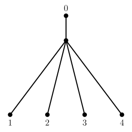
(a)

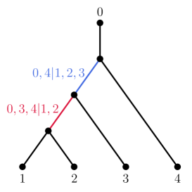
(b)

Figure 2: Two phylogenetic trees with four leaves.

Throughout this paper, we shall use the following notation.

Definition 2.1.

Suppose $N\geq 3$ leaves are given. Let $s$ be a split and $T$ be a phylogenetic tree.

1. $E(T)$ denotes the set of all splits of $T$.

2. $C(s)$ denotes the set of splits compatible with $s$ and $C(T)=\bigcap_{x\in E(T)}C(x)$ the set of splits compatible with the topology of $T$

3. Two sets $A,B$ of splits are compatible if all splits are pairwise compatible.

4. If $s\in C(T)\setminus E(T)$, write $T+\lambda\cdot s$ for the tree obtained by adding the split s to $T\in\mathbb{T}_{N}$ with length $\lambda>0$ and set $T+0\cdot s=T$.

5. $\lvert s\rvert_{T}$ denotes the length of $s$ in $T$ (possibly 0 if the split is not present) and write

   $$\rVert T\lVert:=\sqrt{\sum_{x\in E(T)}\lvert x\rvert_{T}^{2}}\,.$$

2.2 Construction of BHV Spaces: Stratification and the Star Tree $\star$

Next, we briefly introduce Billera-Holmes-Vogtmann tree spaces, giving only essential details. For a formal descirption, see Billera et al. (2001). BHV spaces take split (interior edges) lengths into account, they ignore pendant edges lengths. For $N\in\mathbb{N}$ and $N\geq 3$ there are $M:=2^{N-1}-N-1$ possible splits, so the BHV space $\mathbb{T}_{N}$ of phylogenetic trees with $N$ leaves is the following subset of ${\mathbb{R}}^{M}$: each topology is assigned a corresponding orthant and within, the positive coordinates of a tree with that topology are given by the lengths of its splits. Binary trees are assigned corresponding $(N-2)$-dimensional top-dimensional orthants and non-binary topologies occur at the boundaries of multiple top-dimensional orthants. these orthants. In particular, non-binary topologies occur at the boundaries of multiple orthants. Thus the metric space $(\mathbb{T}_{N},d_{\mathbb{T}_{N}})$ arises from embedding in the Euclidean ${\mathbb{R}}^{M}$, i.e. through gluing the orthants together at these boundaries and carrying the induced intrinsic metric.

Definition 2.2.

For $N\geq 4$ and $1\leq l\leq N-3$, trees with common topology given by the same $N-2-l$ splits, form a stratum $\mathbb{S}\subset\mathbb{T}_{N}$ of codimension $l$. The metric projection onto its closure $\overline{\mathbb{S}}$ is denoted by

$$\operatorname{P}_{\overline{\mathbb{S}}}:\mathbb{T}_{N}\to\overline{\mathbb{S}},\quad T\mapsto\operatorname*{argmin}_{T^{\prime}\in\overline{\mathbb{S}}}d_{\mathbb{T}_{N}}(T,T^{\prime})\,.$$

Remark 2.3.

Every stratum of codimension $1\leq l\leq N-2$, as it corresponds to a $(N-l-2)$-dimensional Euclidean orthant, is convex. In consequence the projection $\operatorname{P}_{\overline{\mathbb{S}}}$ to a closed convex set is well defined.

This construction of Billera et al. (2001) yields a complete metric space $(\mathbb{T}_{N},d)$ of global non-positive curvature – a Hadamard space.

All orthants are open, only the star tree is a single point in BHV space forming the stratum of codimension $N-2$, namely the origin of ${\mathbb{R}}^{M}$. It also acts as the ’origin’ of BHV space, as we will see in Section 2.4. In this work, the star tree plays a key role, and will be denoted by

$$\star\in\mathbb{T}_{N}\,,$$

with trivial metric projection

$$\operatorname{P}_{\{\star\}}:\mathbb{T}_{N}\to\{\star\},\quad T\mapsto\star\,.$$

2.3 Geodesics and Geodesics in BHV spaces

Definition 2.4.

Let $(M,d)$ be a metric space. A continuous curve $\gamma:[a,b]\to M$ is a geodesic if there is a constant $c>0$, called its speed, such that for every $\kappa\in(a,b)$, there is $\epsilon>0$ such that for every $\lambda_{1},\lambda_{2}\in[\kappa-\epsilon,\kappa+\epsilon]$

$$d(\gamma(\lambda_{1}),\gamma(\lambda_{2}))=c\lvert\lambda_{1}-\lambda_{2}\rvert$$

A geodesic is called minimizing if the equation above holds for every $\lambda_{1},\lambda_{2}$. We say a geodesic is of unit speed if $c=1$.

A geodesic segment $G\subseteq M$ is the image of a geodesic, meaning there is a geodesic $\gamma:[a,b]\to M$ such that $G=\gamma([a,b])$.

Let $\gamma:[a,b]\to\mathbb{T}_{N}$ be a continuous curve. Then its length in the above introduced metric $d_{\mathbb{T}_{N}}$ is given by

$$L\left(\gamma\big{|}_{[\lambda_{1},\lambda_{2}]}\right)=\sup_{\begin{subarray}{c}\lambda_{1}\leq t_{1}<\ldots<t_{n}\leq\lambda_{2}\\ n\in\mathbb{N}\setminus\{1\}\end{subarray}}\sum_{i=1}^{n-1}\lVert\gamma(t_{i})-\gamma(t_{i+1})\rVert_{2},$$

where $\gamma_{(}t_{i})$ and $\gamma_{(}t_{i}+1)$ are chosen to lie in the same closed orthant in which $\lVert\cdot\lVert_{2}$ denotes the Euclidean norm. Then, for $T_{1},T_{2}\in\mathbb{T}_{N}$, their distance in $\mathbb{T}_{N}$ is also given by

$$d_{\mathbb{T}_{N}}(T_{1},T_{2})=\min_{\footnotesize\begin{array}[]{c}\gamma:[a,b]\to\mathbb{T}_{N}\mbox{ continuous }\\ \gamma(a)=T_{1},\gamma(b)=T_{2}\end{array}}L(\gamma)\,.$$

Since BHV spaces are Hadamard spaces, as mentioned at the end of the previous Section 2.2, geodesics are unique and so are Fréchet means (Sturm, 2003).

With the notion of ‘support pairs’ Owen (2008) characterize geodesics and Owen and Provan (2011) develop methods to compute geodesics in BHV spaces in polynomial time.

Definition 2.5.

Let $N\geq 3$ and $T_{1},T_{2}\in\mathbb{T}_{N}$. Let $\mathcal{A}=(A_{0},A_{1},\ldots A_{k})$ be a partition of $E(T_{1})\cup(C(T_{1})\cap E(T_{2}))$ and $\mathcal{B}=(B_{0},B_{1},\ldots B_{k})$ be a partition of $E(T_{2})\cup(C(T_{2})\cap E(T_{1}))$.

The pair $(\mathcal{A},\mathcal{B})$ is called a support pair of $T_{1}$ and $T_{2}$ if

1. $A_{0}$ and $B_{0}$ are equal and contain all splits that are either shared between $T_{1}$ and $T_{2}$ or compatible with the other tree, i.e.

   $$A_{0}=B_{0}=\left(E(T_{1})\cap E(T_{2})\right)\cup\left(E(T_{1})\cap C(T_{2})\right)\cup\left(E(T_{2})\cap C(T_{1})\right)\,,$$

   and

2. $A_{i}$ is compatible with $B_{j}$ for all $1\leq j<i\leq k$.

Owen (2011) showed that the geodesic segment joining any two points $T_{1},T_{2}$ corresponds to a unique support pair of the two trees $T_{1},T_{2}$ with the additional property

$$\frac{\|A_{i}\|}{\|B_{i}\|} \leq \frac{\|A_{i+1}\|}{\|B_{i+1}\|},\quad 1\leq i<k\,.$$ (4)

Here,

$$\|A_{i}\|:=\|A_{i}\|_{T_{1}}=\sqrt{\sum_{s\in A_{i}}|s|^{2}_{T_{1}}}\quad\mbox{ and }\quad\|B_{i}\|:=\|B_{i}\|_{T_{2}}=\sqrt{\sum_{s\in B_{i}}|s|^{2}_{T_{2}}}\quad\mbox{ for }1\leq i\leq k\,.$$

Then the geodesic $\overline{\gamma}:[0,1]\to\mathbb{T}_{N}$ with $\overline{\gamma}(0)=T_{1}$ and $\overline{\gamma}(1)=T_{2}$ can be split into the following segments

$$\overline{\gamma}_{i}=\begin{cases}\overline{\gamma}\left(\left[0,\frac{\lVert A_{1}\rVert}{\lVert A_{1}\rVert+\lVert B_{1}\rVert}\right)\right)&\quad\text{if }i=0\,,\\ \overline{\gamma}\left(\left[\frac{\lVert A_{i}\rVert}{\lVert A_{i}\rVert+\lVert B_{i}\rVert},\frac{\lVert A_{i+1}\rVert}{\lVert A_{i+1}\rVert+\lVert B_{i+1}\rVert}\right)\right)&\quad\text{if }1\leq i<k\,,\\ \overline{\gamma}\left(\left[\frac{\lVert A_{i}\rVert}{\lVert A_{i}\rVert+\lVert B_{i}\rVert},1\right]\right)&\quad\text{if }i=k\,,\\ \end{cases}$$

such that $\overline{\gamma}_{i}$ is a straight line in the closed orthant corresponding to the splits of $A_{0}\cup B_{1}\cup\ldots B_{i}\cup A_{i+1}\cup\ldots A_{k}$.

The length of a split $s$ at $\lambda\in[0,1]$ is then given by

$$\lvert s\rvert_{\overline{\gamma}(\lambda)}=\begin{cases}(1-\lambda)\lvert s\rvert_{T_{1}}+\lambda\lvert s\rvert_{T_{2}}\quad&\text{if }s\in A_{0}=B_{0}\,,\\ \frac{(1-\lambda)\lVert A_{i}\rVert-\lambda\lVert B_{i}\rVert}{\lVert A_{i}\rVert}\lvert s\rvert_{T_{1}}\cdot 1_{\left[0,\frac{\|A_{i}\|}{\|A_{i}\|+\|B_{i}\|}\right]}(\lambda)\quad&\text{if }s\in A_{i}\,,1\leq i\leq k\,,\\ \frac{\lambda\lVert B_{i}\rVert-(1-\lambda)\lVert A_{i}\rVert}{\lVert B_{i}\rVert}\lvert s\rvert_{T_{2}}\cdot 1_{\left[\frac{\|A_{i}\|}{\|A_{i}\|+\|B_{i}\|},1\right]}(\lambda)\quad&\text{if }s\in B_{i}\,,1\leq i\leq k\,.\\ \end{cases}$$ (5)

In total, one obtains for the geodesic distance of $T_{1}$ and $T_{2}$

$$d_{\mathbb{T}_{N}}(T_{1},T_{2})=\sqrt{\sum_{s\in A_{0}}(\lvert s\rvert_{T_{1}}-\lvert s\rvert_{T_{1}})^{2}+\sum_{i=1}^{k}(\lVert A_{i}\rVert+\lVert B_{i}\rVert)^{2}}\,.$$ (6)

Vice versa, Owen and Provan (2011) showed that the above construction leads to a geodesic if and only if

$$\frac{\|I_{1}\|}{\|J_{1}\|} > \frac{\|I_{2}\|}{\|J_{2}\|}$$ (7)

for all $i\in\{1,2\ldots,k\}$ and every nontrivial (i.e. each containing at least one element) partitions $A_{i}=I_{1}\cup I_{2}$, $B_{i}=J_{1}\cup J_{2}$ such that $I_{2}$ and $J_{1}$ are compatible.

An illustration of geodesics is given in Figure 3.

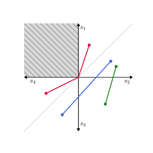
Figure 3: Three examples of geodesics in a subset of $\mathbb{T}_{4}$ from the top point to the bottom point, respectively. The corresponding support pairs are $\big{(}(\emptyset,\{s_{1},s_{2}\}),(\emptyset,\{s_{3},s_{4}\})\big{)}$, $\big{(}(\emptyset,\{s_{1}\},\{s_{2}\}),(\emptyset,\{s_{3}\},\{s_{4}\})\big{)}$ and $\big{(}(\{s_{2}\},\{s_{1}\}),(\{s_{2}\},\{s_{3}\})\big{)}$.

Definition 2.6.

Let $N\geq 3$. For $T_{1},T_{2}\in\mathbb{T}_{N}$, we denote by $\gamma_{T_{1}}^{T_{2}}:[0,d(T_{1},T_{2})]\to\mathbb{T}_{N}$ the unique unit speed geodesic from $T_{1}$ to $T^{\prime}$. The geodesic reparametrized on the unit interval is denoted by $\overline{\gamma}_{T_{1}}^{T_{2}}:[0,1]\to\mathbb{T}_{N}\,,t\mapsto\gamma_{T_{1}}^{T_{2}}(t\cdot d(T_{1},T_{2}))$.

Remark 2.7.

Let $T\in\mathbb{T}_{N}$, $N\geq 3$, and $s$ be an arbitrary split of the appropriate labels. Then, the computation of the distance between $T$ and the tree $\star+\lambda\cdot s$, $\lambda>0$, is rather simple, as is easily verified by (6).We have

$$d^{2}(T,\star+\lambda\cdot s)=\begin{cases}\left(\lambda+\sqrt{\sum_{C(s)\not\ni x\in E(T)}\lvert x\rvert_{T}^{2}}\right)^{2}+\sum_{x\in E(T)\cap C(s)}\lvert x\rvert_{T}^{2}&\text{if }s\not\in C(T)\,,\\ (\lambda-\lvert s\rvert_{T})^{2}+\sum_{s\neq x\in E(T)}\lvert x\rvert_{T}^{2}\quad&\text{if }s\in E(T)\,,\\ \lambda^{2}+\sum_{x\in E(T)}\lvert x\rvert_{T}^{2}&\text{else. }\\ \end{cases}$$

2.4 The Space of Directions and the Tangent Cone

Our results and proposed methods rely on the notion of directions of geodesics. For the following and further reading, we refer to Barden and Le (2018) for orthant spaces, a slightly more general notion of BHV spaces, and (Burago et al., 2001, Chapter 3, 9) for a broader overview in metric geometry.

Definition 2.8.

Let $N\geq 3$ and let $T\in\mathbb{T}_{N}$ and let $\gamma:[0,a]\to\mathbb{T}_{N}$, $\gamma^{\prime}:[0,a^{\prime}]\to\mathbb{T}_{N}$ be two $\gamma(0)=\gamma^{\prime}(0)=T$.

1. The Alexandrov angle at $x$ between $\gamma$ and $\gamma^{\prime}$ is given by

   $$\angle_{T}(\gamma,\gamma^{\prime}):=\lim_{\lambda,\lambda^{\prime}\searrow 0}\arccos\left(\frac{\lambda^{2}+{\lambda^{\prime}}^{2}-d(\gamma(\lambda),\gamma^{\prime}(\lambda^{\prime}))}{2\lambda\cdot\lambda^{\prime}}\right)\,.$$

2. If $\angle_{T}(\gamma,\gamma^{\prime})=0$, the two geodesics have the same direction $\sigma$ at $T$. The space of directions at $T$, denoted by $\Sigma_{T}$, is given by the set of equivalence classes of geodesics with the same directions.

3. The space $\mathfrak{T}_{T}=\Sigma_{T}\times{\mathbb{R}}_{0}/\sim$, where $(\sigma_{1},r_{1})\sim(\sigma_{2},r_{2})$ if $(\sigma_{1}=\sigma_{2}\land r_{1}=r_{2})$ or $(r_{1}=0=r_{2})$, is called the tangent cone at $T$ and it is equipped with the distance

   $$\tilde{d}_{T}((\sigma_{1},r_{1}),(\sigma_{2},r_{2})):=\sqrt{r_{1}^{2}+r_{2}^{2}-2r_{1}r_{2}\cos(\angle_{x}(\sigma_{1},\sigma_{2}))}\,.$$

   The class of $(\sigma,0)$ is called the cone point $\mathcal{O}$.

Remark 2.9.

By construction, the Alexandrov angle confined to the range $[0,\pi]$.

The construction of the spaces of directions and the tangent cone result in two metric spaces.

Proposition 2.10.

Let $N\geq 3$ and $T\in\mathbb{T}_{N}$. Then, both $(\Sigma_{T},\angle_{T})$ and $(\mathfrak{T}_{T},\tilde{d}_{T})$ are complete metric spaces.

From (Bridson and Häfliger, 2011, Theorem II.3.19) we take the following desirable properties.

Remark 2.11.

For any $T\in\mathbb{T}_{N}$, in particular, $(\Sigma_{T},\angle_{T})$ is a CAT(1) space, implying that there are unique geodesics between points of distance $<\pi$. Moreover, $(\mathfrak{T}_{T},\tilde{d}_{T})$ is a Hadamard space.

Definition 2.12.

Let $N\geq 3$.

1. Let $T\in\mathbb{T}_{N}$. For two directions $\sigma,\sigma^{\prime}\in\Sigma_{T}$ with $\angle_{T}(\sigma,\sigma^{\prime})<\pi$, we denote the unit speed geodesic from $\sigma$ to $\sigma^{\prime}$ by $\beta_{\sigma}^{\sigma^{\prime}}:[0,\angle_{T}(\sigma,\sigma^{\prime})]\to\Sigma_{T}$. We write $\overline{\beta}_{\sigma}^{\sigma^{\prime}}:[0,1]\to\Sigma_{T}\,,t\mapsto\beta_{\sigma}^{\sigma^{\prime}}(t\cdot\angle_{T}(\sigma,\sigma^{\prime}))$ for the reparametrized geodesic over the unit interval.

2. For $T\in\mathbb{T}_{N}$, let $\operatorname{dir}_{T}:\mathbb{T}_{N}\setminus\{T\}\to\Sigma_{T}$ denote the map that maps $T^{\prime}\in\mathbb{T}_{N}\setminus\{T\}$ to the direction of the geodesic $\gamma_{T}^{T^{\prime}}$ at $T$.

3. The logarithm map at $T\in\mathbb{T}_{N}$ is defined as

   $$\log_{T}:\mathbb{T}_{N} \to\mathfrak{T}_{T}$$

   $$T^{\prime} \mapsto\begin{cases}\mathcal{O}&\quad\text{if $T=T^{\prime}$,}\\ (\operatorname{dir}_{T}(T^{\prime}),d(T,T^{\prime}))&\quad\text{else.}\end{cases}$$

In view of the above definition of the logarithm we can simply use points in $\mathbb{T}_{N}$ as directions, representing unit speed geodesics from another point in $\mathbb{T}_{N}$ . For instance for $T_{1},T_{2}\in\mathbb{T}_{N}$, $T_{1}\neq T_{2}$ and $\sigma\in\Sigma_{T_{1}}$, we write

$$\angle_{T_{1}}(\sigma,T_{2}):=\angle_{T_{1}}(\sigma,\operatorname{dir}_{T_{1}}(T_{2}))\,.$$

Furthermore, if T is not fully resolved, we write $\sigma_{s}=\operatorname{dir}_{T}(T+1\cdot s)\in\Sigma_{T}$ for a split $s\in C(T)\setminus E(T)$.

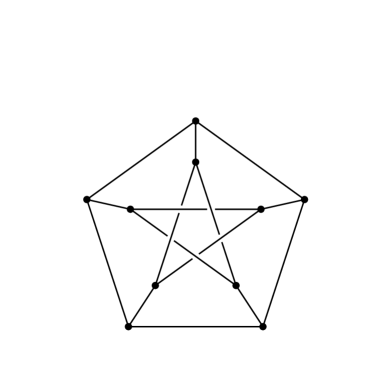
(a)

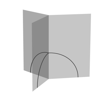
(b)

Figure 4: The link $\mathbb{L}_{4}$ is the Peterson graph, in which each edge has length $\pi/2$.

It turns out that the space of directions at the star tree can be identified with the link,

$$\mathbb{L}_{N}:=\{T\in\mathbb{T}_{N}\ :\ \lVert T\rVert=1\}\,,$$

the unit sphere in BHV spaces. A part of the link in $\mathbb{T}_{4}$ is depicted in Figure 4.

In (Billera et al., 2001, Section 4.1), an alternative way of constructing BHV spaces as cones over the respective links is discussed, with the star tree serving as the cone point. In consequence, the tangent cone at $\star$ is just the space itself, and the link can be identified with the space of directions at $\star$. We condense this in the following proposition.

Proposition 2.13.

Let $N\geq 3$. Then, the following hold.

1. The map $\mathbb{L}_{N}\to\Sigma_{\star},T\mapsto\operatorname{dir}_{\star}(T)$ is bijective.

2. The map $\log_{\star}:\mathbb{T}_{N}\to\mathfrak{T}_{\star}$ is an isometry.

Furthermore, one has for any $T_{1},T_{2}\in\mathbb{T}_{N}\setminus\{\star\}$ that

$$\angle_{\star}\left(\operatorname{dir}_{\star}(T_{1}),\operatorname{dir}_{\star}(T_{2})\right)=\arccos\left(\frac{\lVert T_{1}\rVert^{2}+\lVert T_{2}\rVert^{2}-d^{2}(T_{1},T_{2})}{2\lVert T_{1}\rVert\lVert T_{2}\rVert}\right)\,.$$

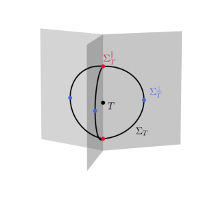
Figure 5: The space of directions at a point $T$ lying in a stratum of codimension 1 in $\mathbb{T}_{4}$. There are two directions parallel and three directions perpendicular to the stratum in which $T$ resides.

The directions perpendicular to a lower dimensional stratum, see Figure 5, play a key role for the limiting behavior of Fréchet means in Theorem 2.16 below and the characterization of their topologies, as we develop in the sequel.

Definition 2.14.

Let $N\geq 3$, $\mathbb{S}\subset\mathbb{T}_{N}$ be a stratum with positive codimension $l\geq 1$ and $T\in\mathbb{S}$. Then we have the directions at $T$perpendicular and parallel to $\mathbb{S}$, respectively, given by

$$\Sigma_{T}^{\perp} :=\{\operatorname{dir}_{T}(T^{\prime})|T^{\prime}\neq T,\ T^{\prime}\in\operatorname{P}_{\overline{\mathbb{S}}}^{-1}(\{T\})\},$$

$$\Sigma_{T}^{\parallel} :=\{\operatorname{dir}_{T}(T^{\prime})|T^{\prime}\neq T,\ T^{\prime}\in\mathbb{S}\}.$$

2.5 The Fréchet Mean in BHV Spaces

Recall the definition of the Fréchet $F_{P}$ function from (1) which is well defined for $P\in\mathcal{P}^{2}\left(\mathbb{T}_{N}\right)$, and the definition of the Fréchet mean set (2), which is well defined for $P\in\mathcal{P}^{1}\left(\mathbb{T}_{N}\right)$ since $\mathbb{T}_{N}$ is complete and, as remarked in the introduction, it is a unique point

$$\mu=\operatorname*{argmin}_{T\in\mathbb{T}_{N}}F_{P}(T)\,,$$

because $\mathbb{T}_{N}$ is a Hadamard space.

Similarly, for a finite set $\mathcal{T}\subset\mathbb{T}_{N}$ of trees, we have the sample Fréchet function

$$F_{\mathcal{T}}(T):=\frac{1}{2|\mathcal{T}|}\sum_{T^{\prime}\in\mathcal{T}}^{n}d^{2}(T,T^{\prime})\,,\quad T\in\mathbb{T}_{N}\,,$$

where $|\mathcal{T}|<\infty$ is the cardinality of $\mathcal{T}$. Also, we have a unique sample mean

$$\hat{\mu}=\operatorname*{argmin}_{T\in\mathbb{T}_{N}}F_{\mathcal{T}}(T)\,.$$

For $P\in\mathcal{P}^{2}\left(M\right)$, $T\in\mathbb{T}_{N}$ and a direction $\sigma\in\Sigma_{T}$, the directional derivative of $F_{P}$ in direction $\sigma$ is given by

$$\nabla_{\sigma}F_{P}(T)=\lim_{\lambda\searrow 0}\frac{F_{P}(\gamma_{T}^{\sigma}(\lambda))-F_{P}(T)}{\lambda}\,,$$

where $\gamma_{T}^{\sigma}:[0,a]\to\mathbb{T}_{N}$ is the unit speed geodesic with $\gamma_{T}^{\sigma}(0)=T$ and direction $\sigma$ at $T$. There is an explicit representation of this derivative and a characterization of the Fréchet mean detailed below.

Theorem 2.15 ((Lammers et al., 2023, Theorems 4.4 and 4.7)).

Let $N\geq 3$, $T\in\mathbb{T}_{N}$ and $P\in\mathcal{P}^{2}\left(\mathbb{T}_{N}\right)$. Then,

• for every $\sigma\in\Sigma_{T}$, we have

  $$\nabla_{\sigma}F_{P}(T)=-\int_{\mathbb{T}_{N}}d(T,T^{\prime})\cos(\angle_{T}(\sigma,\operatorname{dir}_{T}(T^{\prime})))\ \mathrm{d}P(T^{\prime})\,,$$

• the Fréchet mean of $P$ is given by a point $\mu\in\mathbb{T}_{N}$ if and only if

  $$\nabla_{\sigma}F_{P}(\mu)\geq 0\quad\forall\sigma\in\Sigma_{\mu}\,,$$

Unlike the Euclidean case, where equality holds in (ii) of Theorem 2.15, the inequality can be strict in some directions if $\mu$ does not have a fully resolved topology. Notably, it can be strict for all directions at the star tree, or orthogonal to a stratum. In these cases, the behavior of sample means may deviate from the Euclidean law of large numbers as detailed in Theorem 2.16. Such a distribution is called sample sticky, see Lammers et al. (2023, 2023) for this and other "flavors of stickiness".

Theorem 2.16 ((Barden and Le, 2018, Theorem 3, Corollary 7)).

Let $\mathbb{S}\subset\mathbb{T}_{N}$ be a stratum of codimension $l\geq 1$ and $P\in\mathcal{P}^{1}\left(\mathbb{T}_{N}\right)$ with $\mu=\mathfrak{b}(P)\in\mathbb{S}$. For every $\sigma\in\Sigma^{\perp}_{\mu}$, it holds that $\nabla_{\sigma}F_{P}(\mu)\geq 0$.

If further $\nabla_{\sigma}F_{P}(\mu)>0$ for every $\sigma\in\Sigma_{\mu}^{\perp}$, then for every arbitrary sequence $X_{1},X_{2}{\stackrel{{\scriptstyle i.i.d.}}{{\sim}}}P$, there almost surely exists a random $N\in{\mathbb{N}}$ such that

$$\hat{\mu}_{n}\in\mathbb{S}\quad\forall n\geq N\,.$$

For arbitrary Hadamard spaces Sturm (2003) proposed an algorithm computing inductive means that converge in probability to the Fréchet mean, where, under bounded support (e.g. for sample means), convergence is even a.s.: Starting with a first random tree $\hat{\mu}_{0}$, the $j$-th inductive mean $\hat{\mu}_{j}$, $j\in{\mathbb{N}}$ is given traveling the geodesic, parametrized by the unit interval, from $\hat{\mu}_{j-1}$ to the $j$-th random tree $Y_{j}$ only until $\frac{1}{j+1}$. For our purposes here is its sample version.

Data: Trees $T_{1},T_{2},\ldots,T_{n}$

$j\leftarrow 0$;

Draw $Y_{0}\sim\frac{1}{n}\sum_{i=1}\delta_{T_{i}}$ and set $\hat{\mu}_{0}\leftarrow Y_{0}$;

repeat

       $j\leftarrow j+1$;

       Draw $Y_{j}\sim\frac{1}{n}\sum_{i=1}\delta_{T_{i}}$ independent of the $Y_{0},\ldots,Y_{j-1}$;

       $\hat{\mu}_{j}\leftarrow\overline{\gamma}_{\hat{\mu}_{j-1}}^{Y_{j}}\left(\frac{1}{j+1}\right)$;

until convergence;

Algorithm 1 Sturm’s algorithm.

If the Fréchet mean is located on a lower-dimensional stratum, with some trees featuring splits in higher-dimensional strata, compatible to some in the lower dimensional stratum, the output of Sturm’s algorithm will, while metrically close, not necessarily have the correct unresolved topology. This behavior is explained in the following theorem.

Theorem 2.17.

Let $N\geq 3$ and $\mathcal{T}\subset\mathbb{T}_{N}$ be a finite set of trees, with its Fréchet mean $\mu\in\mathbb{S}$ lying in a stratum $\mathbb{S}$ of codimension $l\geq 1$. Let $\hat{\mu}_{j}$, $j\in{\mathbb{N}}$, denote the output of Sturm’s algorithm and suppose that

$$\{T\in\mathcal{T}:\exists s\in E(T)\mbox{ with }s\in C(\mu)\setminus E(\mu)\}\neq\emptyset\,.$$

Then,

$$\mathbb{P}\left(\hat{\mu}_{j}\notin\mathbb{S}\text{ $\infty$-often}\right)=1\,.$$

The goal of the following section will be, first, finding criteria identifying the Fréchet mean’s correct topology, and then, develop algorithms for verification in practice.

3 Finding the Topology of the Fréchet Mean

In this section we first give our main result which at once leads to an algorithm to determine splits present in the topology of a Fréchet sample mean. While the main result is generally applicable to arbitrary strata, for the actual computation, only the corresponding result for the star tree stratum is of concern, and this rewrites in a simple form. The reason, why it suffices to consider star tree strata only is given in the second part where, among others the tangent cone at a stratum is decomposed into a product of the tangent space along the stratum and a product of lower dimensional BHV spaces – of which only their star tree strata are of concern. Essentially, all hinges on directional derivatives orthogonal to the original stratum and for these, the offset inside the stratum is irrelevant.

3.1 A Sufficient Condition for a Split in the Fréchet Mean

While directional derivatives at the Fréchet mean yield a sufficient and necessary condition for a point to be the Fréchet mean, surprsingly, information about its topology can also be obtained from certain directional derivatives at the star tree. Recall the notation $\sigma_{s}=\operatorname{dir}_{T}(T+1\cdot s)\in\Sigma_{T}$ for $T\in\mathbb{T}_{N}$ and $s\in C(T)$.

Theorem 3.1.

Let $N\geq 3$, $\mathbb{S}\subset\mathbb{T}_{N}$ an orthant of codimension $0\leq l<N-2$, $P\in\mathcal{P}^{2}\left(\mathbb{T}_{N}\right)$ with Fréchet mean $\mu\not\in\mathbb{S}$ and $T\in\mathbb{S}$ so that $E(T)\subset E(\mu)$. Then the following hold:

• if $s\in C(T)\setminus E(T)$ with $\angle_{T}(\mu,\sigma_{s}))\geq\pi/2$, then $\nabla_{\sigma_{s}}F_{P}(T)\geq 0$,

• if $\nabla_{\sigma_{s}}F_{P}(T)<0$, then $s\in E(\mu)$.

Remark 3.2.

By Lemma 3.9 in the following section, the directional derivatives do not depend on the particular choice of the point $T\in\mathbb{S}$, only on its topology.

Theorem 3.1 entails the following algorithm for finding splits present in the Fréchet mean’s topology.

Data: trees $\mathcal{T}=\{T_{1},\ldots,T_{n}\}$

$\tilde{\mu}\leftarrow\star$;

$\mathcal{E}\leftarrow\bigcup_{T\in\mathcal{T}}E(T)$;

repeat

       $\tilde{\mu}_{\mathrm{old}}\leftarrow\tilde{\mu}$;

       for $s\in\mathcal{E}$ do

             if $\nabla_{\sigma_{s}}F_{\mathcal{T}}(\tilde{\mu}_{\mathrm{old}})<0$ then

                  $\tilde{\mu}\leftarrow\tilde{\mu}+1\cdot s$;

            

      $\mathcal{E}\leftarrow\mathcal{E}\cap\left(C(\tilde{\mu})\setminus E(\tilde{\mu})\right)$;

      

until $E(\tilde{\mu}_{\textrm{old}})=E(\tilde{\mu})$;

Algorithm 2 An algorithm for finding splits in the Fréchet mean.

Applying Theorem 3.1 to $\mathbb{S}=\{\star\}$ and sample means yields the following.

Corollary 3.3.

Let $\mathcal{T}\subset\mathbb{T}_{N}$ be a finite collection of trees with sample Fréchet mean $\hat{\mu}$. Then, $s\in E(\hat{\mu})$ if

$$\sum_{T\in\mathcal{T}}\sqrt{\sum_{C(s)\not\ni x\in E(T)}\lvert x\rvert_{T}^{2}}<\sum_{T\in\mathcal{T}}\lvert s\rvert_{T}\;.$$ (8)

This result improves a weaker condition from (Anaya et al., 2020, Theorem 5) stating that a split $s\in\cup_{T\in\mathcal{T}}E(T)$ is contained in the sample Fréchet mean if

$$\sum_{T\in\mathcal{T}}\sum_{C(s)\not\ni x\in E(T)}\lvert x\rvert_{T}<\sum_{T\in\mathcal{T}}\lvert s\rvert_{T}\,.$$ (9)

We illustrate the two conditions (8) and (9) by example from (Anaya et al., 2020, Example 1 and 2). While our condition is stronger, it is still not necessary.

Example 3.4.

(Anaya et al., 2020, Example 1) consider the sample mean $\mu$ of four trees $\mathcal{T}=\{T_{1},T_{2},T_{3},T_{4}\}\subset\mathbb{T}_{4}$ as shown in Figure 6 where for $T_{1}$ the split $s_{1}$ has length $w>0$. As there is only one tree, namely $T_{4}\in\mathcal{T}$ having splits not in $C(s_{1})$, (9) is equivalent with

$$10+10=\sum_{x\in E(T_{4})}\lvert x\rvert_{T_{4}}<\sum_{T\in\mathcal{T}}\lvert s_{1}\rvert_{T}=w+3+1\,,$$

i.e. $s_{1}\in\mu$ if $w>16$.

In contrast, (8) rewrites to

$$\sqrt{10^{2}+10^{2}}=\sqrt{\sum_{x\in E(T_{4})}\lvert x\rvert^{2}_{T_{4}}}<\sum_{T\in\mathcal{T}}\lvert s_{1}\rvert_{T}=w+3+1\,,$$

and we obtain the stronger result that $s_{1}\in\mu$ if $w>\sqrt{2}\cdot 10-4\approx 10.142$.

This is, however, not sharp, since direct computation by (Anaya et al., 2020, Example 1) showed that $s_{1}\in\mu$ if $w>9.82$ ( below that and until $9.51$, $\mu=\star$).

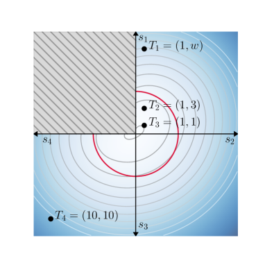
(a)

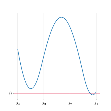
(b)

Figure 6: Illustrating the Fréchet function and its directional derivatives of Example 3.4 in the subspace inhabited by the trees $T_{1},T_{2},T_{3},T_{4}\in\mathbb{T}_{4}$ for the choice $w=10$.

3.2 Tangent Cone and Space of Directions at Lower Dimensional Strata

Let $\mathbb{S}\subset\mathbb{T}_{N}$ be a stratum with positive codimension $l\geq 1$. As was mentioned in Barden and Le (2018), the spaces of directions of points in $\mathbb{S}$ inherits the nature of a stratified space from $\mathbb{T}_{N}$. Theorem 3.7, a more explicit version of (Lammers et al., 2023, Lemma 2), shows how both the spaces of directions and the tangent cone decompose. To this end, introduce the following notion.

Definition 3.5.

For two metric spaces $(M_{1},d_{1}),(M_{2},d_{2})$, their spherical join is given by

$$M_{1}\ast M_{2}=\left[0,\frac{\pi}{2}\right]\times M_{1}\times M_{2}/\sim\ \cong\left\{(\cos\eta\,p_{1},\sin\eta\,p_{2}):0\leq\eta\leq\frac{\pi}{2},p_{i}\in M_{i},i=1,2\right\}\,,$$

i.e. the equivalence class of $(\eta,p_{1},p_{2})$ contains the single point $(\eta,p_{1},p_{2})$ unless $\eta=0,\pi/2$. For $\eta=0$, the class contains all of $M_{2}$ in the last component, hence the class is uniquely determined by $p_{1}\in M_{1}$, and for $\eta=\pi/2$, it contains all of $M_{1}$ in the second component, hence the class is uniquely determined by $p_{2}\in M_{2}$. The spherical join is equipped with the metric

$$d\big{(}(\eta,p_{1},p_{2}),(\eta^{\prime},p_{1}^{\prime},p_{2}^{\prime})\big{)}=\arccos\left(\cos\eta\cos\eta^{\prime}\cos(d_{1}(p_{1},p^{\prime}_{1}))+\sin\eta\sin\eta^{\prime}\cos(d_{2}(p_{2},p^{\prime}_{2}))\right)\,,$$

see e.g. (Bridson and Häfliger, 2011, Definition 5.13).

For metric space $(M_{1},d_{1}),\ldots,(M_{k},d_{k})$, $k\geq 3$ define by induction the nested spherical join

$$M_{1}\ast\Bigg{(}M_{2}\ast\Big{(}M_{3}\ast\big{(}\cdots\ast(M_{k-1}\ast M_{k})\cdots\big{)}\Big{)}\Bigg{)}=\left[0,\frac{\pi}{2}\right]^{k-1}\times M_{1}\times\ldots\times M_{k}/\sim\,.$$

Points, i.e. equivalence classes are determined by their coordinates $(\eta_{1},\ldots,\eta_{k-1},p_{1},\ldots,p_{k})$ with $\eta_{j}\in[0,\pi/2]$, $j=1,\ldots,k-1$, and $p_{j}\in M_{j}$, $j=1,\ldots,k$ and coordinates uniquely determine their points if $\eta_{j}\in(0,\pi/2)$ for all $j=1,\ldots,k-1$. Moreover, $M_{1}$ will be identified with all coordinates having $\eta_{1}=0$, and for $i=2,\ldots,k$, $M_{i}$ will be identified with all coordinates having $\eta_{j}=\pi/2$ for $1\leq j\leq i-1$ and $\eta_{i}=0$.

Remark 3.6.

It is easy to see that the distance between points with coordinates

$$p=(\eta_{1},\ldots,\eta_{k-1},p_{1},\ldots,p_{k}),\quad p^{\prime}=(\eta_{1}^{\prime},\ldots,\eta_{k-1}^{\prime},p_{1}^{\prime},\ldots,p_{k}^{\prime})$$

is then given by

$$d\left(p,p^{\prime}\right) =\arccos\Bigg{(}\sum_{i=1}^{k-1}\ \cos(\eta_{i})\cos(\eta_{i}^{\prime})\left(\prod_{j=1}^{i-1}\sin(\eta_{j})\sin(\eta_{j})^{\prime}\right)d_{i}(p_{i},p_{i}^{\prime})$$

$$\ +\prod_{i=1}^{k-1}\sin(\eta_{i})\sin(\eta_{i})^{\prime}d_{k}(p_{k},p_{k}^{\prime})\Bigg{)}\,.$$ (10)

Theorem 3.7 (Decomposition theorem).

Let $N\geq 3$, $\mathbb{S}\subset\mathbb{T}_{N}$ be a stratum with positive codimension $l\geq 1$ and $T\in\mathbb{S}$. Then the following hold:

• there are $2\geq m\in{\mathbb{N}}$ and BHV spaces ${\mathbb{T}}_{k_{j}}$ of dimensions $1\leq k_{j}$, $j=1,\ldots,m$ with $\sum_{j=1}^{m}(k_{j}-2)=l$ such that the tangent cone and the space of directions at $T$ decompose as follows:

  $$\mathfrak{T}_{T} \cong \mathbb{R}^{N-l-2}\times\mathbb{T}_{k_{1}}\times\cdots\times\mathbb{T}_{k_{m}}$$

  $$\Sigma_{T} \cong \Sigma_{T}^{\parallel}\ast\Sigma_{T}^{\perp}\quad\mbox{ with }\quad\Sigma_{T}^{\parallel}\leavevmode\nobreak\ \cong\leavevmode\nobreak\ S^{N-l-3}\quad\mbox{ and }$$

  $$\Sigma_{T}^{\perp} \cong \mathbb{L}_{k_{1}}\ast\Bigg{(}\mathbb{L}_{k_{2}}\ast\Big{(}\mathbb{L}_{k_{3}}\ast\big{(}\cdots\ast(\mathbb{L}_{k_{m-1}}\ast\mathbb{L}_{k_{m}})\cdots\big{)}\Big{)}\Bigg{)}\,,$$

  where the links are equipped with the Alexandrov angle as metric;

• with the notation from (i), the canonical projections

  $$\varpi_{j}:\mathfrak{T}_{T}\to\mathbb{T}_{k_{j}},\quad j=1,\ldots,m\,,$$

  constructed in the proof of Lemma A.2 in the appendix, and $\sigma=(\eta_{1},\ldots,\eta_{m-1},\sigma_{1},\ldots\sigma_{m})\in\Sigma_{T}^{\perp}$ we have for arbitrary $T^{\prime}\in\mathbb{T}_{N}$ that

  $$d(T,T^{\prime})\cdot\cos(\angle_{T}(\sigma,T^{\prime}))= \sum_{i=1}^{m-1}\left(\prod_{j=1}^{i-1}\sin(\eta_{j})\right)\cos(\eta_{i})\cdot d(\star,\varpi_{i}(\log_{T}(T^{\prime})))\cdot\cos(\angle_{\star}(\sigma_{i},\varpi_{i}(\log_{T}(T^{\prime}))))$$

  $$+\left(\prod_{j=1}^{m-1}\sin(\eta_{j})\right)\cdot d(\star,\varpi_{m}(\log_{T}(T^{\prime})))\cdot\cos(\angle_{\star}(\sigma_{m},\varpi_{m}(\log_{T}(T^{\prime}))))\,.$$

Immediately, we obtain the following corollary.

Corollary 3.8.

Let $N\geq 3$, $\mathbb{S}\subset\mathbb{T}_{N}$ a stratum of codimension $l\geq 1$, $T\in\mathbb{S}$ and $P\in\mathcal{P}^{2}\left(\mathbb{T}_{N}\right)$. Suppose $\mathfrak{T}_{T}\cong{\mathbb{R}}^{N-l-2}\times\mathbb{T}_{k_{1}}\times\ldots\times\mathbb{T}_{k_{m}}$. Then,

$$\nabla_{\sigma}F_{P}(T)\geq 0\quad\forall\sigma\in\Sigma_{T}^{\perp}$$

if and only if for every $i\in\{1,\ldots,m\}$

$$\nabla_{\sigma}F_{P}(T)\geq 0\quad\forall\sigma\in\mathbb{L}_{k_{i}}\subset\Sigma_{T}^{\perp}\,.$$

Since the directions in $\Sigma_{T}^{\perp}$ correspond to the addition of splits that are compatible with the topology of a stratum $\mathbb{S}$, one can naturally identify $\Sigma_{T_{1}}$ with $\Sigma_{T_{2}}$ for $T_{1},T_{2}\in\mathbb{S}$. As the following lemma teaches, the perpendicular directional derivates of the Fréchet function do not depend on the particular reference point in the orthant.

Lemma 3.9 ((Lammers et al., 2023, Corollary 1)).

Let $N\geq 3$ and $\mathbb{S}$ be a stratum of codimension $l\geq 1$. Then, for any $T_{1},T_{2}\in\mathbb{S}$ and $\sigma\in\Sigma_{T_{1}}\cong\Sigma_{T_{2}}$ that

$$\nabla_{\sigma}F_{P}(T_{1})=\nabla_{\sigma}F_{P}(T_{2})\,.$$

4 Minimizing the Directional Derivative

In view of Theorem 2.15, in order to see that a tree $\mu$ is a Fréchet mean of a sample $\mathcal{T}$, we minimize $\nabla_{\sigma}F_{\mathcal{T}}(\mu)$ over $\sigma\in\Sigma_{\mu}$ and show that this minimum is nonnegative. Finding the minimizer, however, requires solving an optimization problem on $\Sigma_{\mu}$. Due to decomposition in Theorem 3.7 it suffices to obtain minima on the star stratum only. The space $\Sigma_{\star}$ inherits the non-smooth nature of the tree space $\mathbb{T}_{N}$. As the number of orthants is given by $(2N-3)!!$, searching for maxima for the direction corresponding to fixed orthants quickly becomes infeasible for larger leaf set sizes.

Deriving a proximal splitting algorithm algorithm and a stochastic gradient algorithm to determining the minimum, instead of traversing all of these many orthants, is the subject of this section.

For a sample $\mathcal{T}=\{T_{1},\ldots T_{n}\},\mathcal{T}\subset\mathbb{T}_{N}$ due to Theorem 2.15, we want to minimize

$$f(\sigma):=\frac{n^{2}\,\nabla_{\sigma}F_{\mathcal{T}}(\star)}{\sum_{j=1}^{N}d(\star,T_{j})}=\sum_{i=1}^{n}w_{i}f_{T_{i}}(\sigma),\quad\sigma\in\Sigma_{\star}$$

where

$$f_{T}(\sigma)=-\cos(\angle_{\star}(\sigma,T)),\quad w_{i}=\frac{d(\star,T_{i})}{\frac{1}{n}\sum_{j=1}^{N}d(\star,T_{j})},\quad i=1,\ldots,n\,.$$

For fixed $0<\nu\leq 1/w_{i}$ for all $i=1,\ldots,n$ (the reason becomes clear in the proof of the Lemma 4.1below), define the proximal splitting operator

$$\operatorname{prox}_{T}(\tau):=\operatorname*{argmin}_{\sigma\in\Sigma_{\star}}\left\{f_{T}(\sigma)+\frac{1}{2\nu}\angle_{\star}(\tau,\sigma)^{2}\right\}\,,\quad\tau\in\Sigma_{\star}\,.$$

The following lemma teaches that $\operatorname{prox}_{T}(\tau)$ is unique and that its computation is rather simple. To this end, recall that $\beta_{\tau}^{{\operatorname{dir}_{\star}(T)}}$ is the geodesic in $\Sigma_{\star}$ mapping $0$ to $\tau$ and $1$ to $T$, while $\bar{\gamma}_{T}^{T^{\prime}}$ is the geodesic in ${\mathbb{T}}_{N}$ mapping $0$ to $T$ and $1$ to $T^{\prime}$.

Lemma 4.1.

For $N\geq 4$, $\tau\in\Sigma_{\star}$, $T\in{\mathbb{T}}\setminus\{\star\}$ with $\angle_{\star}(\operatorname{dir}_{\star}(T),\tau)\in[0,\pi]$ we have

1. $\operatorname{prox}_{T}(\tau)=\left\{\bar{\beta}_{\tau}^{{\operatorname{dir}_{\star}(T)}}(\lambda)\right\}$ where

   $$\lambda=\operatorname*{argmin}_{0\leq\lambda^{\prime}\leq\angle_{\star}(\operatorname{dir}_{\star}(T),\tau)}\left(\bar{\beta}_{\tau}^{{\operatorname{dir}_{\star}(T)}}(\lambda^{\prime})+\frac{\lambda^{2}}{2\nu}\right)\,,$$

   and, in particular $\lambda=0$ in case of $\angle_{\star}(\operatorname{dir}_{\star}(T),\tau)\in\{0,\pi\}$, i.e. $\operatorname{prox}_{T}(\tau)=\left\{\tau\right\}$ then;

2. in case of $\angle_{\star}(\operatorname{dir}_{\star}(T),\tau)<\pi$,

   $$\bar{\beta}_{\tau}^{\operatorname{dir}_{\star}(T)}(\lambda)=\operatorname{dir}_{\star}\left(\overline{\gamma}_{T_{\tau}}^{T/\|T\|}\left(\lambda^{\prime}\right)\right),\quad\lambda\in[0,1]$$

   where $T_{\tau}\in{\mathbb{T}}_{N}$ with $\operatorname{dir}_{\star}(T_{\tau})=\tau$ and $\|T_{\tau}\|=1$, and

   $$\lambda^{\prime}=\frac{\sin(\lambda\cdot\angle_{\star}(\sigma,\tau))}{2\cdot\sin(\angle_{\star}(\sigma,\tau))\cdot\sin\left(\frac{\pi+(1-\lambda)\cdot\angle_{\star}(\sigma,\tau)}{2}\right)}\,,\quad\lambda\in[0,1].$$

We denote by by $p_{T}(\tau)\in\operatorname{prox}_{T}(\tau)$ the unique element for $T\in{\mathbb{T}}_{N},\tau\in\Sigma_{\star}$. The functions $f_{T_{i}}:\{\tau\in\Sigma_{\star}:\angle_{\star}(\tau,\sigma)<\pi/4\}\to{\mathbb{R}}$ are convex as the negative cosine is thus on $[0,pi/2]$, hence we can apply (Lauster and Luke, 2021, Theorem 4) yielding the following assertion for iterates of the corresponding proximal operator on CAT(1) spaces.

Theorem 4.2.

For $N\geq 4$, let $\{T_{1},\ldots,T_{n}\}\subset\mathbb{T}_{N}$ and assume there is a direction $\sigma\in\Sigma_{\star}$ such that $\operatorname{dir}_{\star}(T_{i})\in B_{\pi/4}(\sigma):=\{\tau\in\Sigma_{\star}:\angle_{\star}(\tau,\sigma)<\pi/4\}$ for all $i=1,\ldots,n$, that

$$p: B_{\pi/4}(\sigma)\to B_{\pi/4}(\sigma),\quad\tau\mapsto\Big{(}p_{T_{n}}\circ\ldots\circ p_{T_{1}}\Big{)}(\tau)$$

has a nonempty set of fixed points $\mathrm{Fix}(p)$, and that there is a constant $c>0$ such that $\angle_{\star}(\tau,\mathrm{Fix}(p))<c\cdot\angle_{\star}(\tau,p(\tau))$ for $\tau\in B_{\pi/4}$.Then, for $\tau_{0}\in B_{\pi/4}(\sigma)$ sufficiently close to $\mathrm{Fix}(p)$, the sequence

$$\tau_{m}:=\Big{(}p_{T_{n}}\circ\ldots\circ p_{T_{1}}\Big{)}(\tau_{m-1})\,,\quad m\in{\mathbb{N}}\,,$$

converges to a point in $\mathrm{Fix}(p)$.

Theorem 4.2 as well as Lemma 4.1 motivate the following algorithm.

Data: trees $\mathcal{T}=\{T_{1},\ldots,T_{n}\}$, initial guess $\sigma_{0}$, $0<\nu\leq 1$

$j\leftarrow 0$;

repeat

       $\sigma_{j+1}\leftarrow\operatorname{prox}_{f_{n},\nu}\circ\operatorname{prox}_{f_{n-1},\nu}\circ\ldots\circ\operatorname{prox}_{f_{1},\nu}(\sigma_{j})$;

       $j\leftarrow j+1$

until convergence;

Algorithm 3 A proximal splitting algorithm for finding local minima of $\sigma\mapsto\nabla_{\sigma}F_{\mathcal{T}}(\star)$.

Alternatively, one might use Algorithm 4, inspired by geodesic gradient descent methods. The randomized approach of such an algorithm might be better suited for finding more local minima by ‘exploring’ the space. We do not, however, provide a proof of convergence for this algorithm. The approach here is that, in each iteration, the current position is updated by shooting a geodesic from the current position to a randomly drawn direction from the data set that is less than $\pi$ away.

Data: trees $\mathcal{T}=\{T_{1},\ldots,T_{n}\}$, initial guess $\sigma_{0}$

$j\leftarrow 0$;

repeat

       $I_{j}\leftarrow\{i\in\{1,2,\ldots,n\}:\angle_{\star}(\sigma_{j},T_{i})<\pi\}$;

       Draw $\tau_{j+1}\sim\sum_{i\in I_{j}}\frac{d(\star,T_{i})}{\sum_{l\in I_{j}}d(\star,T_{l})}\delta_{\operatorname{dir}_{\star}{T_{i}}}$;

       $\sigma_{j+1}\leftarrow\overline{\beta}_{\sigma_{j}}^{\tau_{j+1}}\left(\frac{\sin(\angle_{\star}(\sigma_{j},\tau_{j+1}))}{j+1}\right)$;

       $j\leftarrow j+1$:

      

until convergence;

Algorithm 4 An algorithm for finding local minima of $\sigma\mapsto\nabla_{\sigma}F_{\mathcal{T}}(\star)$, inspired by stochastic gradient descent.

Remark 4.3.

By design, Algorithms 3 and 4 are only capable of finding local minima. This is easy to see if the initial guess is ‘isolated’. In each iteration, the current position is updated by going towards a direction from the data set that is less than $\pi$ away. Going back to Example 3.4, starting at $\tau_{0}=\operatorname{dir}_{\star}(T_{4})$, the algorithms would remain stationary at the local minimizer $\operatorname{dir}_{\star}(T_{4})$, regardless of the choice of the parameter $w\geq 1$.

Thus, we recommend using both algorithms multiple times with different initial guesses.

Remark 4.4.

In terms of performance, Algorithm 3 requires fewer computations of angles than Algorithm 4. Determining $I_{j}$ in Algorithm 4 is the major computational bottleneck – it requires the computation of all angles between the current position and the directions from the data set. This can be alleviated by keeping $I_{j}$ for multiple iterations before updating at the cost of precision.

On the other hand, different runs of Algorithm 4 seems to converge against different local minima, whereas Algorithm 3 tends to converge against the same local minimum, see also Figure 9 in Section 6.1.

Since the link $\mathbb{L}_{N}$ stretches across all $(2N-3)!!$ orthants, it can be advisable to perform multiple runs of Algorithm 4 despite the higher computational cost.

5 Hypothesis Testing in the Presence of Stickiness

5.1 Testing for the Presence of Splits in the Fréchet Mean

Building on Theorem 3.1 we derive the following one-sample test for the hypotheses

$$\mathcal{H}_{0}:s\not\in E(\mu)\text{ vs. }\mathcal{H}_{1}:s\in E(\mu)\,,$$ (11)

for the presence of a split $s$ in the population Fréchet mean $\mu$ of probability distribution $P\in\mathcal{P}^{2}\left(\mathbb{T}_{N}\right)$.

Test 5.1 (For the presence of a split in the Fréchet mean).

Given a sample $T_{1},\ldots,T_{n}{\stackrel{{\scriptstyle i.i.d.}}{{\sim}}}P$ and a level $0<\alpha<1$, reject $\mathcal{H}_{0}$ if

$$\hat{Z}:=\frac{\sqrt{n}\,\bar{X}_{n}}{\widehat{\rm sdev}}<c_{\alpha}\mbox{ where }\bar{X}_{n}:=\frac{1}{n}\sum_{i=1}^{n}X_{i},\leavevmode\nobreak\ \widehat{\rm sdev}:=\sqrt{\frac{1}{n-1}\sum_{i=1}^{n}(X_{i}-\bar{X}_{n})^{2}}\,.$$

Here,

$$X_{i}:=-\cos(\angle_{\star}(\sigma_{s},T_{i}))\cdot d(\star,T_{i})\,,\quad i\in\{1,2,\ldots,n\}\,,$$

and $c_{\alpha}$ can be taken as the $\alpha$-quantile of the student $t_{n-1}$-distribution with $n-1$ degrees of freedom, i.e. $\mathbb{P}\{Z\leq c_{\alpha}\}=\alpha$ for $Z\sim t_{n-1}$.

Alternatively, $c_{\alpha}$ can be simulated by bootstrap sampling from the data centered by its sample mean (thereby simulating $\mathcal{H}_{0}$): For $B\in{\mathbb{N}}$ large (typically $1,000$) and each $b=1,\ldots,B$, let $n_{b}\in{\mathbb{N}}$ ($=n$ in $n$-out-of-$n$-bootstrap) sample $X_{1}^{*},\ldots,X_{n_{b}}^{*}{\stackrel{{\scriptstyle i.i.d.}}{{\sim}}}\frac{1}{n}\sum_{i=1}^{n}\delta_{X_{i}-\bar{X}_{n}}$ to obtain

$$Z^{*}_{b}:=\frac{\sqrt{n_{b}}\,\bar{X}^{*}_{b}}{\sqrt{\frac{1}{n_{b}-1}\sum_{i=1}^{n_{b}}(X^{*}_{i}-\bar{X}^{*}_{b})^{2}}},\mbox{ where }\bar{X}^{*}_{b}:=\frac{1}{n_{b}}\sum_{i=1}^{n_{b}}X^{*}_{i}\,,$$

and

$$c_{\alpha}=\max\left\{x\in{\mathbb{R}}:\frac{1}{B}\sum_{b=1}^{B}1_{\left(-\infty,x\right]}\left(Z^{*}_{b}\right)\leq\alpha\right\}\,.$$

Remark 5.2.

1) Since

$$-\cos(\angle_{\star}(\sigma_{s},T))\cdot d(\star,T)=\frac{1}{2}\,\nabla_{s}\,d(\star,T)^{2}\,,$$

for every $T\in\mathbb{T}_{N}$, cf. Theorem 2.15 and thus ${\mathbb{E}}[X_{i}]=\nabla_{s}F_{P}(\star)$ for all $1\leq n$, Test 5.1 is a classical student $t$-test for

$$\mathcal{H}^{\prime}_{0}:\nabla_{s}F_{P}(\star)\geq 0\text{ vs. }\mathcal{H}^{\prime}_{1}:\nabla_{s}F_{P}(\star)<0,$$ (12)

which is robust under nonnormality, i.e. keeping asymptotically the level $\alpha$ (e.g. Romano and Lehmann (2005, Section 11.3)). Although $\nabla_{s}F_{P}(\star)<0$ implies $s\in E(\mu)$, due to Theorem 3.1,$\mathcal{H}^{\prime}_{0}$ may be true without $\mathcal{H}_{0}$ being true, cf. Example 3.4, the true level of Test 5.1 for (11) may be higher than its nominal level, making it more liberal.

2) The necessary condition of Anaya et al. (2020), see Inequality (9), was derived for the Fréchet mean of a finite set of trees. Our improved condition in Theorem 3.1, see Inequality (8), however, is applicable to general probability distributions $P\in\mathcal{P}^{2}\left(\mathbb{T}_{N}\right)$.

We can adapt this test to a more general setting if some splits of the population mean are already known.

Test 5.3 (For the presence of a split in the Fréchet mean if other splits are known).

Given a sample $T_{1},\ldots,T_{n}{\stackrel{{\scriptstyle i.i.d.}}{{\sim}}}P$ and a level $0<\alpha<1$, assume we have have a stratum $\mathbb{S}\subset\mathbb{T}_{N}$ such that for every $T^{\prime}\in\mathbb{S}$, one has $E(T^{\prime})\subset E(\mu)$, where $\mu$ is the unique Fréchet mean of $P$. Further, suppose $s\in C(T^{\prime})$ and $\mathfrak{T}_{T^{\prime}}\cong{\mathbb{R}}^{N-l-2}\times\mathbb{T}_{k_{1}}\times\ldots\times\mathbb{T}_{k_{m}}$ as in Theorem 3.7. Let $\varpi_{r}:\mathfrak{T}_{T}\to{\mathbb{T}}_{k_{r}},r\in\{1,\ldots,m\}$, be the canonical projection such that $\varpi_{r}(T^{\prime}+1\cdot s)\neq\star$. By projecting, we obtain the sample $\mathcal{T}^{\prime}=\{{T^{\prime}_{1}},\ldots,{T^{\prime}_{n}}\}$, where

$$T_{i}^{\prime} =\varpi_{r}(\log_{\mu}(T_{i}))\,,\qquad i=1,\ldots,n\,.$$

Reject $\mathcal{H}_{0}$ from (11) if Test 5.1 rejects $\mathcal{H}^{\prime}_{0}$ (12)for $\mathcal{T}^{\prime}$ and $\sigma_{s}=\operatorname{dir}_{\star}(\varpi_{r}(T^{\prime}+s))$.

5.2 A Two Sample Test for Distributions with Same and Sticky Mean

Building on the central limit theorem for directional derivatives from (Lammers et al., 2023, Theorem 6.1), see also (Mattingly et al., 2024, Theorem 2), for two probability distributions $P,Q\in\mathcal{P}^{2}\left(\mathbb{T}_{N}\right)$ with common Fréchet mean $\mu$ on a stratum $\mathbb{S}$ of codimension $1\leq l\leq N-2$ we propose the following two-sample test for the hypotheses

$$\mathcal{H}_{0}:P=P^{\prime}\text{ vs. }\mathcal{H}_{1}:P\neq P^{\prime}\,,$$ (13)

for the equality of $P$ and $P^{\prime}$, which is motivated by the procedure described in (van der Vaart et al., 1996, Section 3.7.1).

The second test below treats the general case by reducing it via Theorem 3.7 to the special case of $\mathbb{S}=\{\star\}$, treated by the first test below.

Test 5.4 (For equality in the presence of stickiness to $\star$).

Let $\Sigma\subseteq\Sigma_{\star}$.

Given two independent samples $\mathcal{T}=\{T_{1},\ldots,T_{n}\},T_{i}{\stackrel{{\scriptstyle i.i.d.}}{{\sim}}}P$ ($i=1,\ldots,n$) and $\mathcal{T}^{\prime}=\{T^{\prime}_{1},\ldots,T^{\prime}_{n^{\prime}}\}$, $T^{\prime}_{j}{\stackrel{{\scriptstyle i.i.d.}}{{\sim}}}P^{\prime}$ ($j=1,\ldots,n$’), and a level $0<\alpha<1$, let

$$X_{i,\sigma}:=-\cos(\angle_{\star}(\sigma,T_{i}))\cdot d(\star,T_{i})\,,\quad i\in\{1,\ldots,n\}\,,$$

$$X^{\prime}_{j,\sigma}:=-\cos(\angle_{\star}(\sigma,T^{\prime}_{i}))\cdot d(\star,T^{\prime}_{j})\,,\quad j\in\{1,\ldots,n^{\prime}\}\,,$$

Then reject $\mathcal{H}_{0}$ if

$$Z_{(\mathcal{T},\mathcal{T}^{\prime})}:=\sup_{\sigma\in\Sigma}\lvert\bar{X}_{\sigma}-\bar{X}^{\prime}_{\sigma}\rvert>c_{1-\alpha}\mbox{ where }\bar{X}_{\sigma}:=\frac{1}{n}\sum_{i=1}^{n}X_{i,\sigma},\ \bar{X}^{\prime}_{\sigma}:=\frac{1}{n^{\prime}}\sum_{j=1}^{n^{\prime}}X^{\prime}_{j,\sigma}\,.$$

Here, $c_{1-\alpha}$ is obtained through permutation of samples. By sampling from $\mathcal{T}\cup\mathcal{T}^{\prime}$ without replacement, we generate pairs $(\mathcal{T}^{1},{\mathcal{T}^{\prime}}^{1}),\ldots,(\mathcal{T}^{B},{\mathcal{T}^{\prime}}^{B})$, for large $B\in{\mathbb{N}}$ (typically $1,000$) with

$$\lvert\mathcal{T}^{b}\rvert=n\text{ and }\lvert{\mathcal{T}^{\prime}}^{b}\rvert=n^{\prime}\,,\qquad b=1,\ldots,B\,.$$

For these permuted samples, we evaluate the statistics $Z_{(\mathcal{T}^{1},{\mathcal{T}^{\prime}}^{1})},\ldots,Z_{(\mathcal{T}^{B},{\mathcal{T}^{\prime}}^{B})}$ and determine

$$c_{\alpha}=\max\left\{x\in{\mathbb{R}}:\frac{1}{B+1}\left(1+\sum_{b=1}^{B}1_{\left(-\infty,x\right]}\left(Z_{(\mathcal{T}^{b},{\mathcal{T}^{\prime}}^{b})}\right)\right)\leq\alpha\right\}\,.$$

Here, in addition to (van der Vaart et al., 1996, Section 3.7.1) we have added one to the sum in order to avoid p-values of zero (see Belinda and K (2010)). Then, the p-value is given by

$$\mathrm{p}=\frac{1}{B+1}\left(1+\sum_{b=1}^{B}1_{\left(-\infty,x\right]}\left(Z_{(\mathcal{T}^{b},{\mathcal{T}^{\prime}}^{b})}\right)\right)\,.$$

Ideally, one would choose $\Sigma=\Sigma_{\star}$ in Test 5.4. In the absence of suitable numerical methods, this approach quickly becomes computationally infeasible with larger $N$, as the space of directions at the star tree corresponds to a sphere stretching across all $(2N-3)!!$ orthants. Instead, we propose using the following finite selections of directions.

Definition 5.5.

Let $N\geq 3$ and $\mathcal{T},\mathcal{T}^{\prime}\subset\mathbb{T}_{N}$ be two finite subsets of trees. Then let

$$\Sigma_{1} =\{\operatorname{dir}_{\star}(T)\ :\ T\in\mathcal{T}\cup\mathcal{T}^{\prime}\}\,,\text{ and}$$

$$\Sigma_{2} =\{\operatorname{dir}_{\star}(\star+1\cdot s)\ :\ \exists T\in\mathcal{T}\cup\mathcal{T}^{\prime}\mbox{ with }s\in E(T)\}\,.$$

Remark 5.6 (Computational complexity).

Let us briefly discuss the computational complexity of Test 5.4 for both choices of directions. Given a direction $\sigma\in\Sigma_{1}\cup\Sigma_{2}$ (of course this also holds for all $\sigma\in\Sigma_{\star}$), we have that

$$\lvert\bar{X}_{\sigma}-\bar{X}^{\prime}_{\sigma}\rvert=\left\lvert\frac{1}{n}\sum_{i=1}^{n}\lVert T_{i}\rVert\cos(\angle_{\star}(\sigma,T_{i}))-\frac{1}{n^{\prime}}\sum_{j=1}^{n^{\prime}}\lVert T^{\prime}_{j}\rVert\cos(\angle_{\star}(\sigma,T^{\prime}_{j}))\right\rvert\,.$$

Here, the main computational burden lies in computing the angles, which can be done via the Euclidean law of cosines for a tree representing a direction (see Proposition 2.13). For $\Sigma_{2}$ we need to computate of all angles of the type $\angle_{\star}(\star+1s,T)$, $T\in\mathcal{T}\cup\mathcal{T}^{\prime}$. By Remark 2.7, this requires determining the pairwise compatibility of all splits. As each tree has at most $N-2$ splits, the number of splits is bounded from above by $(n+n^{\prime})\cdot(N-2)$. Recall verifying the compatibility $A_{1}|A_{2}$ and $B_{1}|B_{2}$ is done by computing the intersections $A_{i}\cap B_{j}$, $i,j\in\{1,2\}$. Thus, determining the compatibility of two splits is of complexity $\mathcal{O}(N)$. In total, we obtain a complexity of $\mathcal{O}(N^{3}\cdot(n_{x}+n_{y})^{2})$ for computing the pairwise compatibility of the splits.

In case of $\Sigma_{1}$, the directions correspond directly to the data, and thus, all pairwise distances in $\mathcal{T}\cup\mathcal{T}^{\prime}$ need to be computed. As was shown in (Owen and Provan, 2011, Theorem 3.5), computing the distance between two trees is of complexity $\mathcal{O}(N^{4})$. Thus, we obtain a complexity of $\mathcal{O}(N^{4}\cdot(n+n^{\prime})^{2})$ for $\Sigma_{1}$.

Due to the decomposition from Theorem 3.7, we can at once use Test 5.4 to construct the following generally applicable test.

Test 5.7 (For equality in the presence of stickiness to strata).

Given two independent samples $\mathcal{T}=\{T_{1},\ldots,T_{n}\},T_{i}{\stackrel{{\scriptstyle i.i.d.}}{{\sim}}}P$ ($i=1,\ldots,n$) and $\mathcal{T}^{\prime}=\{T^{\prime}_{1},\ldots,T^{\prime}_{n^{\prime}}\},T^{\prime}_{j}{\stackrel{{\scriptstyle i.i.d.}}{{\sim}}}P^{\prime}$ ($j=1,\ldots,n$’), and a level $0<\alpha<1$, let $\mathbb{S}\subset\mathbb{T}_{N}$ be a stratum of codimension $l\geq 1$, $\mu\in\mathbb{S}$ and suppose $\mathfrak{T}_{T}\cong{\mathbb{R}}^{N-l-2}\times\mathbb{T}_{k_{1}}\times\ldots\times\mathbb{T}_{k_{m}}$ as in Theorem 3.7 with canonical projections $\varpi_{r}:\mathfrak{T}_{T}\to{\mathbb{T}}_{k_{r}},r=1,\ldots,m$. Then, we obtain samples $(\mathcal{T}^{r},{\mathcal{T}^{\prime}}^{r})=(\{T_{1}^{r},\ldots,T_{n}^{r}\},\{{\mathcal{T}^{\prime}_{1}}^{r},\ldots,{\mathcal{T}^{\prime}_{n^{\prime}}}^{r}\})$, $r=1,\ldots,m$, where

$$T_{i}^{r} =\varpi_{r}(\log_{\mu}(T_{i}))\,,\qquad i=1,\ldots,n\,,$$

$${\mathcal{T}^{\prime}_{j}}^{r} =\varpi_{r}(\log_{\mu}(T^{\prime}_{j}))\,,\qquad j=1,\ldots n^{\prime}\,,$$

Letting $\mathrm{p}_{r}$ be the p-value obtained from conducting Test 5.4 for the pair of samples $(\mathcal{T}^{r},{\mathcal{T}^{\prime}}^{r})$, $r=1,\ldots,m$, reject $\mathcal{H}_{0}$ if there exists $r\in\{1,2\ldots,m\}$ such that

$$\mathrm{p}_{(r)}<\frac{\alpha}{m+1-r}\,,$$

where $\mathrm{p}_{(1)},\ldots,\mathrm{p}_{(m)}$ are the p-values sorted from lowest to highest, see Holm (1979).

Remark 5.8.

1) Note that $\mu\in\mathbb{S}$ can be arbitrarily chosen.

2) In Brown and Owen (2018), a two sample test was proposed for discriminating two probability distributions in BHV spaces based on the difference of their Fréchet means. If the both distributions are sticky, however, at the star tree, say, the sample Fréchet means will be almost surely exactly at the star tree beyond some random finite sample size (see Theorem 2.16), rendering their approach infeasible in case.

3) While Tests 5.4 and 5.7 have been motivated by the phenomenon of stickiness, they are, of course, applicable for general distributions. In particular, they are very meaningful for cases where both sample Fréchet means are close to the same stratum (yielding finite sample stickiness as discussed by Ulmer et al. (2023)).

6 Applications and Simulations

6.1 Apicomplexa

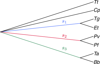
Figure 7: The topology asserted in Nye et al. (2017).

Figure 8: Proposed topologies of the Fréchet mean of the apicomplexa data. The abbreviations stem from the species’ binary nomenclature.

Apicomplexa are a phylum of parasitic alveolates containing a number of important pathogens, such as the causative agents of malaria and toxoplasmosis. The data set we investigate here, originally presented by Kuo et al. (2008) and analyzed by Weyenberg et al. (2017),Nye et al. (2017), consists of 252 rooted trees with 8 taxa (leaves): C. parvum (Cp), T. thermophila (Tt), T. gondii (Tg), E. tenella (Et), P. vivax (Pv), P. falciparum (Rf), B. Bovis (Bb) and T. annulata (Ta).

In particular Nye et al. (2017) determined the Fréchet mean by running Bacák’s algorithm and pruning small edges from the output, resulting in a not fully topology, comprising three splits, namely $s_{1},s_{2},s_{3}$ from Table 1. The topology is also shown in Figure 8.

split	directional derivative	p-value
$s_{1}=\mathrm{Tg},\mathrm{Et}\ \big{|}\ \mathrm{Tt},\mathrm{Cp},\mathrm{Pv},\mathrm{Pf},\mathrm{Ta},\mathrm{Bb}$	$\nabla_{\sigma_{s_{1}}}F_{\mathcal{T}}(\star)\approx-1.2\cdot 10^{-4}$	$<10^{-15}$
$s_{2}=\mathrm{Pv},\mathrm{Pf}\ \big{|}\ \mathrm{Tt},\mathrm{Cp},\mathrm{Tg},\mathrm{Et},\mathrm{Ta},\mathrm{Bb}$	$\nabla_{\sigma_{s_{2}}}F_{\mathcal{T}}(\star)\approx-3.4\cdot 10^{-4}$	$<10^{-15}$
$s_{3}=\mathrm{Ta},\mathrm{Bb}\ \big{|}\ \mathrm{Tt},\mathrm{Cp},\mathrm{Tg},\mathrm{Et},\mathrm{Pv},\mathrm{Pf}$	$\nabla_{\sigma_{s_{3}}}F_{\mathcal{T}}(\star)\approx-2.1\cdot 10^{-1}$	$<10^{-15}$

Table 1: Splits (first column) comprising the Fréchet mean of the apicomplexa data set from Kuo et al. (2008) in Section 6.1; splits $s_{1},s_{2},s_{3}$ have been found by Nye et al. (2017). The second column lists their directional derivatives (negative values imply presence in the mean). The last column shows the p-values of the corresponding one-sample tests Test 5.1 first three tests were numerically indistinguishable from 0.

We verified the presence of these splits in the sample Fréchet mean by showing that the corresponding directional derivatives are negative at the star tree (cf. Theorem 3.1).

Algorithms 3 and 4 were run for a hundred different initial orthogonal directions pointing to data, where these directions have been projected according to Theorem 3.7. They were not able to find a negative directional derivative, indicating that the non-fully resolved topology $E(\mu)=\{s_{1},s_{2},s_{3}\}$ for the Fréchet mean $\mu$ is indeed correct. Their outputs are displayed in Figure 9.

We used the implementation of Sturm’s algorithm of Miller et al. (2015) 1000 times on our data set with default configurations. Despite the Fréchet mean being unresolved, all 1000 proposals for the Fréchet mean were fully resolved, which is not coming as a surprise in light of Theorem 2.17. The splits $s_{1},s_{2},s_{3}$ were present in all 1000 outputs. Besides these three splits, we observed 8 other splits in total. Amongst them, two splits stood out: the splits $\mathrm{Tt},\mathrm{Cp}\ \big{|}\ \mathrm{Tg},\mathrm{Et},\mathrm{Pv},\mathrm{Pf},\mathrm{Ta},\mathrm{Bb}$ and $\mathrm{Tg},\mathrm{Et},\mathrm{Tt},\mathrm{Cp}\ \big{|}\ \mathrm{Pv},\mathrm{Pf},\mathrm{Ta},\mathrm{Bb}$ were present in 990 and 986 out of 1000 trees, respectively, despite not being in the correct topology we determined. The other splits were featured less than ten times. This highlights that caution is required when dealing with the output of Sturm’s algorithm, as even multiple runs on the same data can lead to misleading conclusions.

After having determined the topology of the sample mean, we infer on the topology of the population mean. To this end we conduct Test 5.4 three times at level $0.05$ to test the hypotheses

$$\mathcal{H}_{1}^{\prime} :\nabla_{\sigma_{s_{1}}}F_{P}(\star)\geq 0\,,\quad\mathcal{H}_{2}^{\prime}:\nabla_{\sigma_{s_{2}}}F_{P}(\star)\geq 0\,,\quad\mathcal{H}_{3}^{\prime}:\nabla_{\sigma_{s_{3}}}F_{P}(\star)\geq 0\,.$$

After a Holm’s correction Holm (1979), we can reject all three hypotheses at level 0.05. By Theorem 3.1, this implies the presence of splits $s_{1},s_{2},s_{3}$ in the population Fréchet mean.

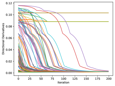
(a)

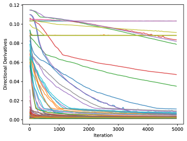
(b)

Figure 9: Directional derivatives for the apicomplexa data set. Each colored line represents starting at one of the first 100 trees: no directions with negative derivative were found.

6.2 Brain Arteries and Cortical Landmarks

In Skwerer et al. (2014), brain artery trees were analyzed by mapping them to points in BHV tree space. In human brains, (usually) four brain artery trees emerge from the circle of Willis. They reconstructed these subtrees from Magnetic Resonance images and artificially connected these to a root, creating a single brain artery tree. Furthermore, 128 labelled correspondence points on the cortex were determined and then connected to the closest vertex in the brain artery tree. All non-labeled leaves were then pruned, resulting in rooted 85 trees with 128 labelled leaves. Computing BHV sample Fréchet means via Sturm’s algorithm, they observed that the output was very close to the star tree but did not converge, even after 50,000 iterations. Rather the topology frequently changed in the last iterations, indicating the star tree to be the mean of the data.

S. Skwerer and J. S. Marron provided 84 of such trees (one had to be removed) which we split into two data sets corresponding to 41 male and 44 female patients. We performed Algorithm 4 on both data sets as shown in Figure 10. Our analysis suggests that the Fréchet mean of both data sets is indeed the star tree. Our two sample tests could not detect a difference between male and female brain trees, which in the light of finding a significant but not highly significant difference by topological data analysis methods suggest that sex differences seem less distinct.

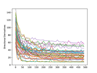
(a)

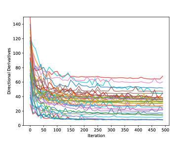
(b)

Figure 10: Due to the rather high leafcount of 128, we chose to perform multiple runs of Algorithm 4 for different initial positions, c.f. Remark 4.4. The results support the claim that the star tree is the Fréchet mean of both data sets corresponding to male and female patients: we did not find negative directional derivatives.

6.3 Stickiness and Hybridization in Baboon Populations

We saw in Theorem 2.16 that the Fréchet mean of a distribution sticks to a lower-dimensional stratum if and only if the directional derivatives in directions perpendicular to the stratum are non-negative. This, by Corollary 3.8, is equivalent to stickiness at the star tree in lower-dimesional tree space.

By Theorems 2.15 and 2.16, a distribution $P\in\mathcal{P}^{2}\left(\mathbb{T}_{N}\right)$ sticks to the star tree $\star\in\mathbb{T}_{N}$ if and only if

$$0<\int-d(\star,T)\cdot\cos(\angle_{\star}(\sigma,T))\,dP(T)\quad\forall\sigma\in\Sigma_{\star}\,.$$

Therefore, distributions that are spread across multiple orthants of very different topologies, will generally tend to have negative directional derivatives.

A biological factor that could lead to such a distribution is hybridization. Hybridization (or interbreeding between populations) gives rise to lateral gene transfer between different species. A hybridization event is often modelled as a subtree prune and regraft (SPR) operation on phylogenies: a subtree is removed from a tree and reattached to another edge (see e.g. Allen and Steel (2000) or Hein (1990)).

Depending on the gene sequence and the species involved, the effect of hybridization on the inferred phylogenetic tree can lead to trees that are very close in terms of the SPR distance (see e.g. Baroni et al. (2005)), but far away in BHV distance. To undo such a SPR operation in the BHV space, one would need to shrink at least all splits connecting the subtree to its previous position, before regrowing the now missing edges. An effect of hybridization in a data set of trees can then be that the Fréchet mean becomes non-fully resolved and, most likely, sticky.

The data set we investigate here is a collection of 4260 trees with 19 taxa. 18 of the taxa are baboon populations, and the 19th taxon is an outgroup. The Fréchet mean of the data set was found to be the star tree, even failing to detect the outgroup. The data set was provided by the DPZG and was previously analyzed in Sørensen et al. (2023). There, it was found that hybridization occured between the baboon populations, most likely causing topological heterogeneity between gene trees, and leading to the unresolved Fréchet sample mean. Nevertheless, the directional derivatives of the Fréchet function at the star tree might still be useful in the presence of hybridization.

We computed the median of the overall lengths of the trees and split the data set accordingly into trees from slower- and faster-evolving genetic loci. The output of Sturm’s algorithm for both data sets appeared to be the star tree, motivating a two sample test. We conducted Test 5.4 based on the directional derivatives of the Fréchet function at the star tree. We considered directions corresponding to single splits and performed 49998 random permutations. The p-value was estimated to be $\approx 2\cdot 10^{-5}$, indicating that the two groups differ significantly, see Figure 11. Although this division of the data set by total evolutionary length is artificial, it illustrates how our two-sample test can be applied to experimental data.

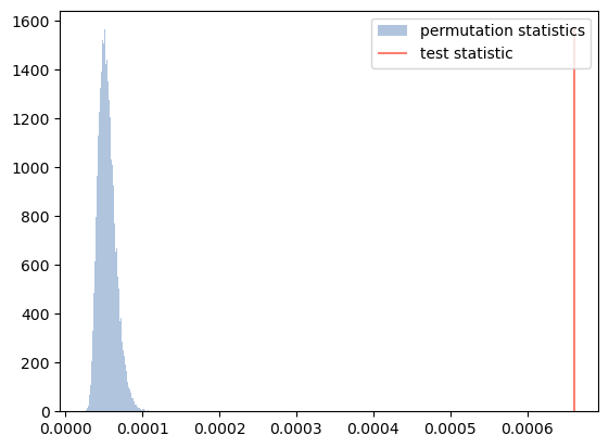
Figure 11: A histogram for the values of the test statistic after 49998 random permutations of the 4260 trees.

6.4 Simulations for the Two-Sample Test

For the two-sample test, we conducted a number of simulations to investigate the power of the test in different scenarios. We compared the different choices of directions against each other and against a permutation test based with the Wasserstein distance as test statistic.

Using the Wasserstein distance as test statistic is motivated by the work of Lammers et al. (2023) and Lammers et al. (2023), where the authors proved that stickiness of distributions corresponds to robustness of the Fréchet mean against small changes in the Wasserstein space of probability distributions, i.e. every other distribution that is sufficiently close in Wasserstein distance has a Fréchet mean lying on the same stratum.

We can observe in the experiments displayed in Figure 12, that tests based on the directional derivatives appear to be more powerful than tests based on the Wasserstein distance. Figure 12(a) shows that this result depends considerably on the choice of directions, all choices outperform the Wasserstein distance in the more anisotropic case of Figure 12(b).

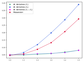
(a)

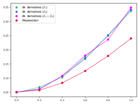
(b)

Figure 12: In both numerical experiments, two samples in $\mathcal{T},\mathcal{T}^{\prime}\subset\mathbb{T}_{4}$ were generated, both having an equal sample size $\lvert\mathcal{T}\rvert=\lvert\mathcal{T}^{\prime}\rvert=50$. For both samples, the topologies were drawn uniformly and the edge lengths in the first sample follow exponential distributions with scale 1. Figure 12(a) and Figure 12(b) correspond to two different ways of drawing the edge lengths of the second sample. The level for all tests was set to $0.05$.

It appears, however, that the test is not optimal for discrete probability distributions as can be seen in Figure 13. In this scenario, the test based on the Wasserstein distance easily outperforms the tests based on directional derivatives. For such distributions, a Wasserstein based test might be more appropriate.

We also want to highlight that our test has a computational advantage. For each permutation, the evaluation of the Wasserstein distance requires solving a linear program, whereas our test statistic only requires summation and subtraction of the permuted directional derivatives.

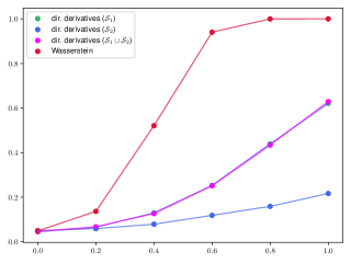
Figure 13: In these numerical experiments, two samples in $\mathcal{T},\mathcal{T}^{\prime}\subset\mathbb{T}_{4}$ were generated, both having an equal sample size $\lvert\mathcal{T}\rvert=\lvert\mathcal{T}^{\prime}\rvert=50$. For both samples, the edge lengths are fixed at 1. The topology of the first sample were drawn uniformly. For the second sample, three predetermined topologies were drawn with probability $(1+\lambda\cdot 4)/15$, the remaining topologies with probability $(1-\lambda)/15$. The parameter was chosen from $\lambda\in\{0,0.2,0.4,0.6,0.8,1\}$.

7 Discussion

In this paper we have illustrated that despite the attractive features of BHV tree space, use of the Fréchet mean can be challenging due to (i) computational issues calculating the sample mean and (ii) stickiness of the population mean affecting asymptotic tests.

The new sufficient condition we have derived for presence of edges in the Fréchet mean tree applies to both sample and population means. As illustrated in Example 3.4, this condition is a strict improvement on the condition in (Anaya et al., 2020, Theorem 1).

Our rigorous test and algorithm for identifying splits in the population and sample mean is a statistically valid method as opposed to arbitrary removal of short edges, illustrated by the Apicomplexa example and the brain data example.

Further, our new two-sample test can distinguish distributions which share the same sticky mean, illustrated by the baboon example.

The baboon data also suggests a link between lack of resolution and underlying biological mechanisms such as populations believed to have undergone extensive hybridization. The effect on gene trees can be represented by SPR which results in highly dispersed samples in BHV tree space and unresolved Fréchet means. Although lack of resolution in the Fréchet mean suggests a loss of information (e.g. the sample mean does not move when data change), the directional derivatives of the Fréchet function may retain information about the biological processes relating species trees to gene trees.

Appendix A Proofs

A.1 Proof of Theorem 2.17

Proof.

Let $Y_{j},j\in{\mathbb{N}}$ be the sequence of i.i.d. random variables that is used to generate the inductive means $\hat{\mu}_{j}$ of Sturm’s algorithm. By hypothesis there is a split $s$ such that

$$\mathcal{T}_{s}:=\{T\in\mathcal{T}:E(T)\ni s\in C(\mu)\setminus E(\mu)\}\neq\emptyset\,.$$

Further, by construction, if $\hat{\mu}_{k-1}\in\mathbb{S}$ and $Y_{j}\in\mathcal{T}_{s}$. i.e. $|s|_{Y_{j}}=\lambda$ for some $\lambda>0$, then $|s|_{\hat{\mu}_{j}}=\frac{\lambda}{j+1}$ by (5), i.e. $\hat{\mu}_{j}\notin\mathbb{S}$. In consequence

$$\{\hat{\mu}_{j-1}\in\mathbb{S},Y_{j}\in\mathcal{T}_{s}\} \subseteq \{\hat{\mu}_{j}\notin\mathbb{S}\}\,.$$ (14)

Since

$$\sum_{j=1}^{\infty}\mathbb{P}\{Y_{j}\in\mathcal{T}_{s}\}=\sum_{j=1}^{\infty}\frac{\lvert\mathcal{T}_{s}\rvert}{|\mathcal{T}|}=\infty\,,$$

application of the Borell-Cantelli Lemma, e.g. Durrett (2019, Theorem 2.3.7), yields in conjunction with (14), as asserted:

$$1=\mathbb{P}\{Y_{j}\in\mathcal{T}_{s}\,\infty\mbox{ often}\}\leq\mathbb{P}\{\hat{\mu}_{j}\not\in\mathbb{S}\,\infty\mbox{ often}\}\,.$$

∎

A.2 Proof of Theorem 3.1

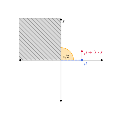
(a)

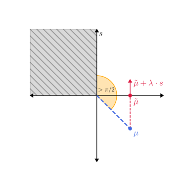
(b)

Figure 14: An illustration of cases 1 and 3 in the proof of Theorem 3.1 in $\mathbb{T}_{4}$.

We first show that (i) implies (ii). Indeed, negating the statement in (i), we obtain $\nabla_{\sigma_{s}}F_{P}(T)<0\implies\angle_{T}(\sigma_{s},\mu)<\pi/2$. This, in turn, implies that $\mu$ lies in an stratum bordering $T+1s$. Since $E(T)\subset E(\mu)$, trees in the stratum of $\mu$ must contain $s\in E(\mu)$, yielding (ii).

Next we show (i). By Lemma 3.9, the directional derivative $\nabla_{\sigma_{s}}F_{P}(T)$ does not depend on the position of $T\in\mathbb{S}$. Therefore, we can assume that $T=\operatorname{P}_{\overline{\mathbb{S}}}(\mu)\in\mathbb{S}$. We distinguish between three cases, see Figure 14 for visualisations of cases 1 and 3.

Case 1: $\angle_{T}(\mu,s)=\pi/2$.

If $\angle_{T}(\mu,\sigma_{s})=\pi/2$, the topology of $\mu$ cannot be fully resolved and $s\in C(\mu)$. Therefore, it follows that $\nabla_{\sigma_{s}}F_{P}(\mu)\geq 0$ by Theorem 2.15. Now, let $\gamma_{T}^{\mu}$ denote the unit speed geodesic from $T$ to $\mu$. By Lemma 3.9,we also have for every $\kappa\in(0,d(T,\mu)]$ that $\nabla_{\sigma_{s}}F_{P}(\gamma_{T}^{\mu}(\kappa))=\nabla_{\sigma_{s}}F_{P}(\mu)\geq 0$. Since $F_{P}$ is convex, e.g. (Sturm, 2003, proof of Proposition 4.3), the derivative traversing from $\gamma_{T}^{\mu}(\kappa)$ in direction $\sigma_{s}$ is nondecreasing, i.e. for all $\lambda>0$ and all $\kappa\in(0,d(T,\mu)]$, we have $F_{P}(\gamma_{T}^{\mu}(\kappa))\leq F_{P}(\gamma_{T}^{\mu}(\kappa)+\lambda\cdot s)\,.$ Taking the limit $\kappa\to 0$, we obtain by continuity of $F_{P}$ that $F_{P}(T)\leq F_{P}(T+\lambda\cdot s)$. Thus,

$$\nabla_{\sigma_{s}}F_{P}(T)=\lim_{\lambda\searrow 0}\frac{F_{P}(T+\lambda\cdot s)-F_{P}(T)}{\lambda}\geq 0\,.$$

Case 2: $\angle_{T}(\mu,\sigma_{s})=\pi$.

In this case, the unit speed geodesic $\gamma_{\mu}^{T+1\cdot s}$ from $\mu$ to $T+1\cdot s$ passes through the star tree. As $\mu$ is the unique minimizer of the convek $F_{P}$, the function $F_{P}\circ\gamma_{\mu}^{T+1\cdot s}$ is non-decreasing. Consequently, we have that

$$\nabla_{\sigma_{s}}F_{P}(T)=\lim_{\lambda\searrow 0}\frac{F_{P}\big{(}\gamma_{\mu}^{T+1\cdot s}(d(T,\mu)+\lambda)\big{)}-F_{P}(\overbrace{\gamma_{\mu}^{T+1\cdot s}(d(T,\mu)}^{=T})}{\lambda}\geq 0\,.$$

Case 3: $\pi/2<\angle_{T}(\mu,\sigma_{s})<\pi$.

In this case, $s$ must be compatible with some the splits in $E(\mu)\setminus E(T)$ but not with all of them. Consider the tree $\tilde{\mu}$ obtained by removing the splits of $\mu$ incompatible with $s$. At $\tilde{\mu}$, we have that $\angle_{\tilde{\mu}}(\sigma_{s},\mu)=\pi$ due to the incompatibility of $s$ and the deleted splits. Since $\angle_{\tilde{\mu}}(\sigma_{s},\mu)=\pi$, the geodesic $\gamma_{\mu}^{\tilde{\mu}+1\cdot s}$ must pass through $\tilde{\mu}$. Furthermore, since $\mu$ is the unique Fréchet mean, $F_{P}\circ\gamma_{\mu}^{\tilde{\mu}+1\cdot s}$ is non-decreasing. Hence, $\nabla_{s}F_{P}(\tilde{\mu})\geq 0$.

Next, consider the geodesic $\gamma_{T}^{\tilde{\mu}}$. Again, we have that for every $\kappa\in(0,d(T,\tilde{\mu})]$ that $\nabla_{\sigma_{s}}F_{P}(\gamma_{T}^{\tilde{\mu}}(\kappa))=\nabla_{\sigma_{s}}F_{P}(\tilde{\mu})\geq 0$. Consequently, we have for every $\lambda>0$ and $\kappa\in(0,d(T,\tilde{\mu})]$ by the convexity of $F_{P}$ that $F_{P}(\gamma_{T}^{\tilde{\mu}}(\kappa))\leq F_{P}(T+\lambda\cdot s)$ Taking the limit $\kappa\to 0$, we see $F_{P}(T)\leq F_{P}(T+\lambda\cdot s)$ for every $\lambda>0$. Thus, $\nabla_{\sigma_{s}}F_{P}(T)\geq 0$, which is assertion (i). ∎

A.3 Proof of Corollary 3.3

The Fréchet function at the star tree is given by

$$F_{\mathcal{T}}(\star)=\frac{1}{2\cdot\lvert\mathcal{T}\rvert}\sum_{T\in\mathcal{T}}\sum_{x\in E(T)}\lvert x\rvert_{T}^{2}\,.$$

Furthermore, by Remark 2.7

$$2\cdot\lvert\mathcal{T}\rvert\cdot F_{\mathcal{T}}(\star+\lambda\cdot s)=\quad \sum_{\footnotesize\begin{array}[]{c}T\in\mathcal{T}\\ s\in E(T)\end{array}}\left((\lambda-\lvert s\rvert_{T})^{2}+\sum_{s\neq x\in E(T)}\lvert x\rvert_{T}^{2}\right)+\sum_{\footnotesize\begin{array}[]{c}T\in\mathcal{T}\\ s\in C(T)\\ s\not\in E(T)\end{array}}\left(\lambda^{2}+\sum_{x\in E(T)}\lvert x\rvert_{T}^{2}\right)$$

$$+ \sum_{\footnotesize\begin{array}[]{c}T\in\mathcal{T}\\ s\not\in C(T)\end{array}}\left(\left(\lambda+\sqrt{\sum_{C(s)\not\ni x\in E(T)}\lvert x\rvert_{T}^{2}}\right)^{2}+\sum_{\footnotesize\begin{array}[]{c}x\in E(T)\\ x\in C(s)\end{array}}\lvert x\rvert_{T}^{2}\right)\,.$$

Thus, we get

$$F_{\mathcal{T}}(\star+\lambda\cdot s)-F_{\mathcal{T}}(\star)=\frac{\lambda^{2}}{2}+\frac{\lambda}{\lvert\mathcal{T}\rvert}\cdot\left(\sum_{T\in\mathcal{T}}\sqrt{\sum_{C(s)\not\ni x\in E(T)}\lvert x\rvert_{T}^{2}}-\sum_{T\in\mathcal{T}}\lvert s\rvert_{T}\right)\,.$$

And hence

$$\nabla_{\sigma_{s}}F_{\mathcal{T}}(\star)=\frac{1}{\lvert\mathcal{T}\rvert}\left(\sum_{T\in\mathcal{T}}\sqrt{\sum_{C(s)\not\ni x\in E(T)}\lvert x\rvert_{T}^{2}}-\sum_{T\in\mathcal{T}}\lvert s\rvert_{T}\right)\,.$$

Theorem 3.1 then yields the claim. ∎

A.4 Proof of Theorem 3.7

We first state and show two auxiliary lemmata and then prove the theorem.

Lemma A.1.

Let $T\in\mathbb{S}$. If $\mathbb{T}_{N}\ni T^{\prime}\in\operatorname{P}_{\overline{\mathbb{S}}}^{-1}(\{T\})$, we have $\lvert s\rvert_{T}=\lvert s\rvert_{T^{\prime}}$ for every $s\in E(T)$.

Proof.

Let $(A_{0},\ldots A_{k})$, $(B_{0},\ldots B_{k})$ be the support pair of the geodesic from $T$ to $T^{\prime}$.

If $E(T)\subseteq E(T^{\prime})$, due to (6), the distance is given by

$$d(T,T^{\prime})=\sqrt{\sum_{s\in E(T)}(\lvert s\rvert_{T}-\lvert s\rvert_{T^{\prime}})^{2}+\sum_{s\in E(T^{\prime})\setminus E(\tilde{T})}\lvert s\rvert_{T^{\prime}}^{2}}\,.$$

The first term $\sum_{s\in E(T)}(\lvert s\rvert_{T}-\lvert s\rvert_{T^{\prime}})^{2}$ is minimal if and only if it is 0. Hence, the claim follows.

Next, assume that $E(T)\not\subseteq E(T^{\prime})$. As $E(T)\neq E(T)\cap E(T^{\prime})$, there is $i\in\{1,2,\ldots,k\}$ such that $\lVert A_{i}\rVert_{T}>0$. Define $\widetilde{T}\in\overline{\mathbb{S}}$ with $E(\widetilde{T})=E(T)\cap E(T^{\prime})$ by $\lvert s\rvert_{\tilde{T}}=\lvert s\rvert_{T^{\prime}}$ for all $s\in E(\widetilde{T})$. By definition, it holds $\bigcup_{i=1}^{k}B_{i}=E(T^{\prime})\setminus E(T)=E(T^{\prime})\setminus E(\tilde{T})$. Thus, we obtain, again by (6),

$$d(T,T^{\prime}) =\sqrt{\sum_{s\in A_{0}}(\lvert s\rvert_{T_{1}}-\lvert s\rvert_{T_{1}})^{2}+\sum_{i=1}^{k}(\lVert A_{i}\rVert+\lVert B_{i}\rVert)^{2}}\geq\sqrt{\sum_{i=1}^{k}(\lVert A_{i}\rVert+\lVert B_{i}\rVert)^{2}}$$

$$>\sqrt{\sum_{i=1}^{k}\lVert B_{i}\rVert^{2}}=\sqrt{\sum_{s\in E(T^{\prime})\setminus E(\tilde{T})}\lvert s\rvert_{T^{\prime}}^{2}}=d(\tilde{T},T^{\prime})\,,$$

a contradiction to the assumption that $P_{\overline{\mathbb{S}}}(T^{\prime})=T\neq\widetilde{T}$.

∎

We will also need the following Lemma, c.f. (Owen, 2011, Theorem 2.1).

Lemma A.2.

Let $N\geq 4$ and $T_{1},T_{2}\in\mathbb{T}_{N}$. Let $\mathcal{E}\subseteq E(T_{1})\cap E(T_{2})$. Then, there are lower dimensional BHV spaces ${\mathbb{T}}_{k_{j}}$ of dimensions $k_{j}$ and pairs of trees $(T_{1}^{j},T_{2}^{j})$, $j=1,\ldots,|\mathcal{E}|+1$ such that

1. $T_{1}^{j},T_{2}^{j}\in\mathbb{T}_{k_{j}}$ for all $j\in\{1,2,\ldots,|\mathcal{E}|+1\}$,

2. $\sum_{j=1}^{|\mathcal{E}|+1}(k_{j}-2)=(N-2)-|\mathcal{E}|$,

3. $d^{2}(T_{1},T_{2})=\sum_{s\in\mathcal{E}}(\lvert s\rvert_{T_{1}}-\lvert s\rvert_{T_{2}})^{2}+\sum_{j=1}^{|\mathcal{E}|+1}d^{2}(T_{1}^{j},T_{2}^{j})$.

Proof.

If $\mathcal{E}=\emptyset$ the assertion is trivial. Hence we now assume that $\lvert\mathcal{E}\rvert=:m\geq 1$. We will then iteratively construct the tuples $(T_{1}^{j},T_{2}^{j})$, $j=1,\ldots,\mathcal{E}$ by bisection at common splits $s\in\mathcal{E}$.

Suppose the root’s label is 0. We begin by choosing a split

$$A|B=s\in\operatorname*{argmin}_{\begin{subarray}{c}C|D\in\mathcal{E}\,,\\ 0\in D\end{subarray}}\lvert C\rvert\,.$$ (15)

By (Owen, 2011, Theorem 2.1), bisection of $T_{1},T_{2}$ at the shared split $s$ yields four trees $(T_{1}^{1},T_{2}^{1}),(\widetilde{T}_{1}^{1},\widetilde{T}_{2}^{1})$, where a new leaf $v$ is added in lieu of the deleted split: the set of leaves of $T_{1}^{1},T_{2}^{1}$ is given by $A$ and $v$ serves as root, the set of leaves of $\widetilde{T}_{1}^{1},\widetilde{T}_{2}^{1}$ is $(B\setminus\{0\})\cup\{v\}$ where $0$ remains the root. Setting $k_{1}:=\lvert A\rvert$, and $\tilde{k}_{1}:=\lvert B\rvert-1+1$, (Owen, 2011, Theorem 2.1) showed that $T_{1}^{1},T_{2}^{1}\in\mathbb{T}_{k_{1}}$, $\widetilde{T}_{1}^{1},\widetilde{T}_{2}^{1}\in\mathbb{T}_{\tilde{k}_{1}}$,

$$d^{2}(T_{1},T_{2})=\left(\lvert s\rvert_{T_{1}}-\lvert s\rvert_{T_{2}}\right)^{2}+d^{2}\left(T_{1}^{1},T_{2}^{1}\right)+d^{2}\left(\widetilde{T}_{1}^{1},\widetilde{T}_{2}^{1}\right)\,,$$ (16)

and we add at once that

$$(k_{1}-2)+(\tilde{k}_{1}-2)=\lvert A\rvert+\lvert B\rvert-4=(N-2)-1\,.$$ (17)

If $m=1$, setting $k_{2}=\tilde{k}_{1}$, and $T_{i}^{2}:=\widetilde{T}_{i}^{1}$ for $i=1,2$, the assertion follows from (16) and (17).

In case of $m>1$, we choose the next split

$$A^{\prime}|B^{\prime}=s^{\prime}\in\operatorname*{argmin}_{\begin{subarray}{c}C|D\in\mathcal{E}\setminus\{s\}\,,\\ 0\in D\end{subarray}}\lvert C\rvert\,.$$

Since $s,s^{\prime}$ are compatible, $0\in B\cap B^{\prime}$ and $B\cap A^{\prime}x=\emptyset\overset{A^{\prime}\subset A\cup B}{\implies}A^{\prime}\subset A$, yielding a contradiction to minimality of $A$ in (15), only one of the following two cases holds

1. $A\cap A^{\prime}=\emptyset\overset{A\subset A^{\prime}\cup B^{\prime}}{\implies}A\subset B^{\prime}\setminus\{0\}$ and $A^{\prime}\subset B\setminus\{0\}$

2. $A\cap B^{\prime}=\emptyset\overset{B\subset A^{\prime}\cup B^{\prime}}{\implies}A\subset A^{\prime}$ and $B^{\prime}\subset B$.

Recalling that $\widetilde{T}_{i}^{1}$ are trees over the leaf set $(B\setminus\{0\})\cup\{v\}$ with root $0$, in case of (a) the split $s^{\prime}$ corresponds to the split $\widetilde{s}^{\prime}:=A^{\prime}|(B^{\prime}\setminus A)\cup\{v\}$ of $\widetilde{T}_{i}^{1}$, $i=1,2$; whereas in case (b) it corresponds to $\widetilde{s}^{\prime}:=(A^{\prime}\setminus A)\cup\{v\}|B^{\prime}$. Deleting this split results in a new vertex $v^{\prime}$ and, once again invoking (Owen, 2011, Theorem 2.1), we obtain four trees (see Figure 15:

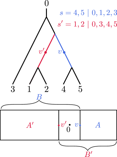
(a)

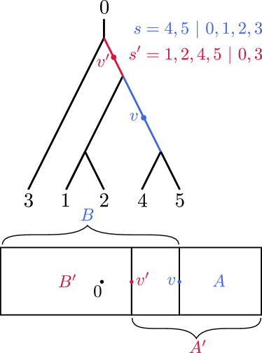
(b)

Figure 15: Schematic display of split sets for the trees in the proof of Lemma A.2 with examples on the top. Left: case (a), right: case (b)

The first two are $T^{2}_{1},T^{2}_{2}\in{\mathbb{T}}_{k_{2}}$ with leaf set $A^{\prime}$ (case (a)) and $(A^{\prime}\setminus A)\cup\{v\}$ (case (b)), respectively, with new root $v^{\prime}$, where we have set $k_{2}:=\lvert A^{\prime}\lvert$ (case (a)) and $k_{2}:=\lvert A^{\prime}\rvert-\lvert A\rvert+1$ (case (b)), respectively.

The other two trees are $\widetilde{T}^{2}_{1},\widetilde{T}^{2}_{2}\in{\mathbb{T}}_{\widetilde{k}_{2}}$ with leaf set $(B^{\prime}\cup\{v,v^{\prime}\})\setminus A$ (case (a)) and $B^{\prime}\cup\{v^{\prime}\}$ (case (b)), respectively, with root $0$, where we have set $\widetilde{k}_{2}:=\lvert B^{\prime}\rvert-\lvert A\rvert+1$ (case (a)) and $:=\lvert B^{\prime}\lvert$ (case (b)), respectively. Due to (Owen, 2011, Theorem 2.1), we obtain

$$d^{2}(\widetilde{T}^{1}_{1},\widetilde{T}^{1}_{2})=\left(\lvert\widetilde{s}^{\prime}\rvert_{\widetilde{T}^{1}_{1}}-\lvert\widetilde{s}^{\prime}\rvert_{\widetilde{T}^{1}_{2}}\right)^{2}+d^{2}\left(T_{1}^{2},T_{2}^{2}\right)+d^{2}\left(\widetilde{T}_{1}^{2},\widetilde{T}_{2}^{2}\right)\,,$$ (18)

and at once

$$(k_{2}-2)+(\tilde{k}_{2}-2)=\lvert A^{\prime}\rvert+\lvert B^{\prime}\rvert-\lvert A\rvert-3=N+1-k_{1}-3=N-2-2-(k_{1}-2)\,.$$ (19)

If $m=2$, setting $k_{3}:=\tilde{k}_{2}$, and $T_{i}^{3}:=\widetilde{T}_{i}^{2}$ for $i=1,2$, the assertion follows from (16), (17), (18) and (17), since $\lvert\widetilde{s}^{\prime}\rvert_{\widetilde{T}^{1}_{i}}=\lvert s^{\prime}\rvert_{T_{i}}$ for $i=1,2$.

If $m>2$ iteration of the above step for all remaining splits in $\mathcal{E}\setminus\{s,s^{\prime}\}$ yields the assertion.

∎

Proof of Theorem 3.7. As shown in (Lammers et al., 2023, Lemma 2), we have $\Sigma_{T}=\Sigma_{T}^{\parallel}\ast\Sigma_{T}^{\perp}$. Since $\mathbb{S}$ is isometric to a Euclidean orthant of dimension $m=N-l-2$, one has by the definition of $\Sigma_{T}^{\parallel}$ that $\Sigma_{T}^{\parallel}\cong S^{N-l-3}$. Therefore, we are left to understand the structure of $\Sigma_{T}^{\perp}$. Let $\sigma_{1},\sigma_{2}\in\Sigma_{T}^{\perp}$ with corresponding geodesics $\overline{\gamma}_{1},\overline{\gamma}_{2}:[0,1]\to\mathbb{T}_{N}$ starting at $T$ with directions $\sigma_{1},\sigma_{2}$, respectively. We set $T_{i}=\gamma_{i}(1)$, $i=1,2$. By definition of $\Sigma_{T}^{\perp}$, we have that $T_{1},T_{2}\in\operatorname{P}_{\overline{\mathbb{S}}}^{-1}(\{T\})$. We know by Lemma A.1 that

$$\lvert T_{1}\rvert_{s}=\lvert T_{2}\rvert_{s}=\lvert T\rvert_{s}$$ (20)

for all $s\in E(T)$. In particular, we have $E(T)\subset E(T_{1})\cap E(T_{2})$.

Now Next, we apply Lemma A.2 (for notation purposes further below, we take recourse to additional tildes here) for $T_{1},T_{2}$ and $\mathcal{E}=E(T)$, giving us pairs of trees $(\widetilde{T}_{1}^{j},\widetilde{T}_{2}^{j})\in{\mathbb{T}}_{\tilde{k}_{j}}$, $j=1,\ldots,\lvert E(T)\rvert+1$ such that

$$\sum_{j=1}^{\lvert E(T)\rvert+1}(\tilde{k}_{j}-2)=N-2-\lvert E(T)\rvert=l\,,$$ (21)

and

$$d^{2}(T_{1},T_{2})=\sum_{s\in\mathcal{E}}(\lvert s\rvert_{T_{1}}-\lvert s\rvert_{T_{2}})^{2}+\sum_{j=1}^{\lvert E(T)\rvert+1}d^{2}(\widetilde{T}_{1}^{j},\widetilde{T}_{2}^{j})\stackrel{{\scriptstyle\eqref{eq:same_lengths}}}{{=}}\sum_{j=1}^{\lvert E(T)\rvert+1}d^{2}(\widetilde{T}_{1}^{j},\widetilde{T}_{2}^{j})\,.$$ (22)

At this point, we might have some $\tilde{k}_{j}=2$ for some $j\in\{1,\ldots,\lvert E(T)\rvert+1\}$. As ${\mathbb{T}}_{2}$ only contains its star tree one then has $d(\widetilde{T}_{1}^{j},\widetilde{T}_{2}^{j})=0$. Thus, neither does such $\tilde{k}_{j}$ contribute to (21) nor do the trees $\widetilde{T}_{1}^{j},\widetilde{T}_{2}^{j}\in{\mathbb{T}}_{\tilde{k}_{j}}$ contribute to (22).

Therefore, we can safely remove every $\tilde{k}_{j}=2$, yielding $k_{1},\ldots k_{m}$ and $(T_{1}^{j},T_{2}^{j})\in{\mathbb{T}}_{k_{j}}$ with $j=1,2,\ldots,m$ and $m\leq E(T)+1$ such that

$$\sum_{j=1}^{m}(k_{j}-2)=l\,,$$ (23)

and

$$d^{2}(T_{1},T_{2})=\sum_{j=1}^{m}d^{2}(T_{1}^{j},T_{2}^{j})\,.$$ (24)

Another application of Lemma A.2 for $T$ and $T_{i}$, $i=1,2$, since $\mathcal{E}=E(T)$ and hence $T^{j}=\star\in{\mathbb{T}}_{k_{j}}$ for all $j=1,\ldots,m$ yields at once

$$d^{2}(T,T_{i})=\sum_{j=1}^{m}d^{2}(\star,T_{i}^{j})\,.$$ (25)

We have by (6) that

$$d(T,\gamma_{i}^{j}(\lambda))=\sqrt{\sum_{s\in E(T_{i})\setminus E(T)}\lvert s\rvert^{2}_{\gamma_{i}(\lambda))}}=\lambda\cdot\sqrt{\sum_{s\in E(T_{i})\setminus E(T)}\lvert s\rvert^{2}_{T_{i}}}=\lambda\cdot d(T,T_{i})\,,\quad i=1,2\,.$$ (26)

Next, let $(\mathcal{A},\mathcal{B})$ with $\mathcal{A}=(A_{0},\ldots,A_{k})$, $\mathcal{B}=(B_{0},\ldots,B_{k})$ be the support pair of the geodesic between $T_{1},T_{2}$. Note that since $E(T)\subset E(T_{i})\subseteq C(T)$ for $i=1,2$, for every $\lambda\in(0,1]$, one has $E(\gamma_{i}(\lambda))=E(T_{i})$, $i=1,2$. Then, we have for every $\lambda\in(0,1]$ and $j=1,2,\ldots,k$

$$\lVert A_{j}\rVert_{\gamma_{1}(\lambda)}=\lambda\cdot\lVert A_{j}\rVert_{T_{1}}\text{ and }\lVert B_{j}\rVert_{\gamma_{2}(\lambda)}=\lambda\cdot\lVert B_{j}\rVert_{T_{2}}\,,$$ (27)

and consequently

$$\frac{\lVert A_{r}\rVert_{\gamma_{1}(\lambda)}}{\lVert B_{r}\rVert_{\gamma_{2}(\lambda)}}=\frac{\lVert A_{r}\rVert_{T_{1}}}{\lVert B_{r}\rVert_{T_{2}}}\,,\quad r=1,\ldots,k\,.$$

Now, (4) and (7), similarly (7) for $T_{1},T_{2}$ implies at once its validity for $\gamma_{1}(\lambda),\gamma_{2}(\lambda)$ for all $\lambda\in(0,1]$, yield that $(\mathcal{A},\mathcal{B})$ must also be the support pair of the geodesic between $\gamma_{1}(\lambda)$ and $\gamma_{2}(\lambda)$ for all $\lambda\in(0,1]$. Again by (6), we have

$$d(\gamma_{1}(\lambda),\gamma_{2}(\lambda)) = \sqrt{\sum_{s\in A_{0}}(\lvert s\rvert_{\gamma_{2}(\lambda)}-\lvert s\rvert_{\gamma_{1}(\lambda)})^{2}+\sum_{r=1}^{k}(\lVert A_{r}\rVert_{\gamma_{1}(\lambda)}+\lVert B_{r}\rVert_{\gamma_{2}(\lambda)})^{2}}$$ (28)

$$\stackrel{{\scriptstyle\eqref{eq:same_lengths}}}{{=}} \sqrt{\sum_{s\in A_{0}\setminus E(T)}(\lvert s\rvert_{\gamma_{2}(\lambda)}-\lvert s\rvert_{\gamma_{1}(\lambda)})^{2}+\sum_{r=1}^{k}(\lVert A_{r}\rVert_{\gamma_{1}(\lambda)}+\lVert B_{r}\rVert_{\gamma_{2}(\lambda)})^{2}}$$

$$\stackrel{{\scriptstyle\eqref{eq:pull-out-lambda}}}{{=}} \lambda\cdot\sqrt{\sum_{s\in A_{0}\setminus E(T)}(\lvert s\rvert_{T_{1}}-\lvert s\rvert_{T_{1}})^{2}+\sum_{r=1}^{k}(\lVert A_{r}\rVert_{T_{1}}+\lVert B_{r}\rVert_{T_{2}})^{2}}$$

$$= \lambda\cdot d(T_{1},T_{2})\,.$$

Let $\sigma_{i}^{j}=\operatorname{dir}_{\star}(T_{i}^{j})$ for $i=1,2$ and $j=1,2,\ldots,m$. Then

$$\cos(\angle_{T}(\sigma_{1},\sigma_{2})) = \lim_{\lambda\searrow 0}\frac{d^{2}(T,\gamma_{1}(\lambda))+d^{2}(T,\gamma_{2}(\lambda))-d^{2}(\gamma_{1}(\lambda),\gamma_{2}(\lambda))}{2d(T,\gamma_{1}(\lambda))d(T,\gamma_{2}(\lambda))}$$ (29)

$$\stackrel{{\scriptstyle\eqref{eq:scale_dist_to_T}\text{ and }\eqref{eq:scale_dist_between}}}{{=}} \frac{d^{2}(T,T_{1})+d^{2}(T,T_{2})-d^{2}(T_{1},T_{2})}{2d(T,T_{1})d(T,T_{2})}$$

$$\stackrel{{\scriptstyle\eqref{eq:distance_orth_trimmed}\text{ and }\eqref{eq:distance_orth_reference}}}{{=}} \sum_{j=1}^{m}\frac{d(\star,T_{1}^{j})}{d(T,T_{1})}\frac{d(\star,T_{2}^{j})}{d(T,T_{2})}\frac{d^{2}(\star,T_{1}^{j})+d^{2}(\star,T_{2}^{j})-d^{2}(T_{1}^{j},T_{2}^{j})}{2d(\star,T_{1}^{j})d(\star,T_{2}^{j})}$$

$$= \sum_{j=1}^{m}\frac{d(\star,T_{1}^{j})}{d(T,T_{1})}\frac{d(\star,T_{2}^{j})}{d(T,T_{2})}\cdot\cos\left(\angle_{\star}\left(\sigma_{1}^{j},\sigma_{2}^{j}\right)\right)$$

Now, set for $i\in\{1,2\}\,,j\in\{1,2,\ldots,m-1\}$

$$\eta_{i}^{j}=\begin{cases}0&\text{if }d(\star,T_{i}^{j})=0\,,\\ \arccos\left(\frac{d(\star,T_{i}^{j})}{\sqrt{d^{2}(T,T_{i})-\sum_{r<j}d^{2}(\star,T_{i}^{r})}}\right)\quad&\text{ else.}\end{cases}$$ (30)

Note that $\eta_{i}^{j}\in[0,\pi]$ since

$$d^{2}(\star,T_{i}^{j})+\sum_{r<j}d^{2}(\star,T_{i}^{r})=\sum_{r=1}^{j}d^{2}(\star,T_{i}^{r})\leq\sum_{r=1}^{m}d^{2}(\star,T_{i}^{r})\stackrel{{\scriptstyle\eqref{eq:distance_orth_reference}}}{{=}}d^{2}(T,T_{i})$$

$$\Leftrightarrow$$

$$\frac{d(\star,T_{i}^{j})}{\sqrt{d^{2}(T,T_{i})-\sum_{r<j}d^{2}(\star,T_{i}^{r})}}\leq 1\,.$$

Hence, we have

$$\sin(\eta_{i}^{j})=\sqrt{1-\cos^{2}(\eta_{i}^{j})}=\sqrt{1-\frac{d^{2}(\star,T_{i}^{j})}{d^{2}(T,T_{i})-\sum_{k<j}d^{2}(\star,T_{i}^{k})}}=\sqrt{\frac{d^{2}(T,T_{i})-\sum_{k\leq j}d^{2}(\star,T_{i}^{k})}{d^{2}(T,T_{i})-\sum_{k<j}d^{2}(\star,T_{i}^{k})}}$$

Then, we have for $i=1,2$ and $1\leq j<m$:

$$\cos(\eta_{i}^{j})\cdot\prod_{k=1}^{j-1}\sin(\eta_{i}^{k}) =\frac{d(\star,T_{i}^{j})}{\sqrt{d^{2}(T,T_{i})-\sum_{\ell<j}d^{2}(\star,T_{i}^{\ell})}}\cdot\prod_{k=1}^{j-1}\sqrt{\frac{d^{2}(T,T_{i})-\sum_{\ell\leq k}d^{2}(\star,T_{i}^{\ell})}{d^{2}(T,T_{i})-\sum_{\ell<k}d^{2}(\star,T_{i}^{\ell})}}$$

$$=\frac{d(\star,T^{j}_{i})}{d(T,T_{i})}\,,$$

and

$$\prod_{k=1}^{m-1}\sin(\eta_{i}^{k})=\frac{\sqrt{d^{2}(T,T_{i})-\sum_{\ell\leq m-1}d^{2}(\star,T_{i}^{\ell})}}{d(T,T_{i})}\stackrel{{\scriptstyle\eqref{eq:distance_orth_reference}}}{{=}}\frac{d(\star,T^{m}_{i})}{d(T,T_{i})}\,,$$

Thus, (29) becomes

$$\cos(\angle_{T}(\sigma_{1},\sigma_{2})) =\sum_{j=1}^{m}\left(\prod_{k=1}^{j-1}\sin(\eta_{1}^{k})\sin(\eta_{2}^{k})\right)\cos(\eta_{1}^{j})\cos(\eta_{2}^{j})\cdot\cos\left(\angle_{\star}\left(\sigma_{1}^{j},\sigma_{2}^{j}\right)\right)$$

$$\quad+\left(\prod_{k=1}^{m-1}\sin(\eta_{1}^{k})\sin(\eta_{2}^{k})\right)\cdot\cos\left(\angle_{\star}\left(\sigma_{1}^{m},\sigma_{2}^{m}\right)\right)\,,$$ (31)

revealing the structure from (3.6) of a nested spherical join:

$$\Sigma_{T}^{\perp}\cong\mathbb{L}_{k_{1}}\ast\Bigg{(}\mathbb{L}_{k_{2}}\ast\Big{(}\mathbb{L}_{k_{3}}\ast\big{(}\cdots\ast(\mathbb{L}_{k_{m-1}}\ast\mathbb{L}_{k_{m}})\cdots\big{)}\Big{)}\Bigg{)}\,.$$

The structure of the tangent cone follows from (Bridson and Häfliger, 2011, Proposition I.5.15). Let $C_{0}M$ denote the Euclidean cone over a metric space $M$, c.f. (Bridson and Häfliger, 2011, Definiton I.5.6). Then, by

$$\mathfrak{T}_{T}=C_{0}\Sigma_{T} \cong C_{0}S^{N-l-3}\times C_{0}\Sigma_{T}^{\perp}$$

$$\cong{\mathbb{R}}^{N-l-2}\times C_{0}\left(\mathbb{L}_{k_{1}}\ast\Bigg{(}\mathbb{L}_{k_{2}}\ast\Big{(}\mathbb{L}_{k_{3}}\ast\big{(}\cdots\ast(\mathbb{L}_{k_{m-1}}\ast\mathbb{L}_{k_{m}})\cdots\big{)}\Big{)}\Bigg{)}\right)$$

$$\cong{\mathbb{R}}^{N-l-2}\times C_{0}\mathbb{L}_{k_{1}}\times C_{0}\Bigg{(}\mathbb{L}_{k_{2}}\ast\Big{(}\mathbb{L}_{k_{3}}\ast\big{(}\cdots\ast(\mathbb{L}_{k_{m-1}}\ast\mathbb{L}_{k_{m}})\cdots\big{)}\Big{)}\Bigg{)}$$

$$\ \vdots$$

$$\cong{\mathbb{R}}^{N-l-2}\times C_{0}\mathbb{L}_{k_{1}}\times\cdots\times C_{0}\mathbb{L}_{k_{1}}$$

$$\stackrel{{\scriptstyle\text{Proposition \ref{prop:bhv_cone}}}}{{\cong}}{\mathbb{R}}^{N-l-2}\times{\mathbb{T}}_{k_{1}}\times\cdots\times{\mathbb{T}}_{k_{m}}\,.$$

Now, let us pick $\sigma_{1}:=\sigma=(\eta_{1}^{1},\ldots,\eta_{1}^{m-1},\sigma_{1},\ldots,\sigma_{m})\in\Sigma_{T}^{\perp}$. As an element in $\Sigma_{T}$, it is given by $(0,\sigma_{1}^{\parallel},\sigma_{1})$, where $\sigma_{1}^{\parallel}\in\Sigma_{T}^{\parallel}$ is arbitrary.

Next, we decompose down $\sigma_{2}:=\operatorname{dir}_{T}(T,T^{\prime})$. Let $\mathfrak{T}^{\perp}_{T}:=C_{0}\Sigma_{T}^{\perp}$ and let $\varpi_{\perp}:\mathfrak{T}_{T}\to\mathfrak{T}_{T}^{\perp}$ denote the canonical projection. Writing $\sigma_{2}$ as element of $\Sigma^{\parallel}\ast\Sigma_{\perp}$, one has $\sigma_{2}=(\eta_{0}^{i},\sigma_{2}^{\parallel},\sigma_{2}^{\perp})$, where for the origin $\mathcal{O}\in\mathfrak{T}_{T}^{\perp}$

$$\eta_{0}^{1}=\arccos\left(\frac{d(\mathcal{O},\varpi_{\perp}(\log_{T}(T^{\prime})))}{d(T,T^{\prime})}\right)\,.$$

Then, we obtain by the definition of spherical joins

$$d(T,T^{\prime})\cdot\cos(\angle_{T}(\sigma,T^{\prime})) = d(T,T^{\prime})\cos(\eta_{0}^{1})\cdot\cos(\angle_{\mathcal{O}}(\sigma,\varpi_{\perp}(T^{\prime})))$$ (32)

$$= d(\mathcal{O},\varpi_{\perp}(\log_{T}(T^{\prime})))\cdot\cos(\angle_{\mathcal{O}}(\sigma,\varpi_{\perp}(T^{\prime})))$$

At last, we prove (ii). As $\mathfrak{T}^{\perp}_{T}\cong{\mathbb{T}}_{k_{1}}\times\cdot{\mathbb{T}}_{k_{m}}$, we have

$$d(\mathcal{O},\varpi_{\perp}(\log_{T}(T^{\prime}))=\sum_{i=1}^{m}d^{2}(\star,\varpi_{i}(\log_{T}(T^{\prime})))\,,$$

The orthogonal directions $\Sigma_{T}^{\perp}$ correspond to the addition of splits that are compatible with the topology. In particular, $\sigma_{2}^{\perp}$ corresponds to the the addition of splits in $T^{\prime}$ that are compatible with the splits of $T$.

Thus, we can identify $\varpi_{\perp}(\log_{T}(T^{\prime}))$ with the tree ${T^{\prime}}^{\perp}:=T+\sum_{s\in C(T)\setminus E(T)}\lvert s\rvert_{T^{\prime}}\cdot s$.

In particular, we have $\sigma_{2}^{\perp}=\operatorname{dir}_{T}$ and $d(\mathcal{O},\varpi_{\perp}(\log_{T}(T^{\prime}))=d(T,{T^{\prime}}^{\perp})$. Another application of Lemma A.2 for $T,{T^{\prime}}^{\perp}$ and $\mathcal{E}=E(T)$ then yields the explicit trees ${T^{\prime}}^{i}=\varpi_{j}(\log_{\mu}(T^{\prime}))\in{\mathbb{T}}_{k_{j}}$, $j=1,\ldots,m$, and we have, as before,

$$\sigma_{2}^{\perp}=(\eta_{2}^{1},\ldots,\eta_{2}^{m-1},\operatorname{dir}_{\star}({T^{\prime}}^{1},\ldots,{T^{\prime}}^{m})\,,$$

where for $j=1,\ldots,m$

$$\eta_{2}^{j}=\begin{cases}0&\text{if }d(\star,(T^{j})=0\,,\\ \arccos\left(\frac{d(\star,{T^{\prime}}^{j})}{\sqrt{d^{2}(T,{T^{\prime}}^{\perp})-\sum_{r<j}d^{2}(\star,{T^{\prime}}^{j})}}\right)\quad&\text{ else.}\end{cases}$$

Finally, we obtain

$$\frac{d(T,T^{\prime})}{d(T,\varpi_{\perp}(\log_{T}(T^{\prime})))} \cdot \cos(\angle_{T}(\sigma,wT^{\prime}))\stackrel{{\scriptstyle\eqref{eq:perp_pull}}}{{=}}\cos(\angle_{\mathcal{O}}(\sigma,\varpi_{\perp}(T^{\prime})))$$

$$\stackrel{{\scriptstyle\eqref{eq:join-distance-proof-theorem}}}{{=}} \sum_{j=1}^{m}\left(\prod_{k=1}^{j-1}\sin(\eta_{1}^{k})\sin(\eta_{2}^{k})\right)\cos(\eta_{1}^{j})\cos(\eta_{2}^{j})\cdot\cos\left(\angle_{\star}\left(\sigma_{1}^{j},\sigma_{2}^{j}\right)\right)$$

$$+\left(\prod_{k=1}^{m-1}\sin(\eta_{1}^{k})\sin(\eta_{2}^{k})\right)\cdot\cos\left(\angle_{\star}\left(\sigma_{1}^{m},\sigma_{2}^{m}\right)\right)\,,$$

$$= \sum_{i=1}^{m-1}\left(\prod_{j=1}^{i-1}\sin(\eta_{j})\right)\cos(\eta_{i})\cdot\frac{d(\star,\varpi_{i}(\log_{T}(T^{\prime})))}{d(T,\varpi_{\perp}(\log_{T}(T^{\prime})))}\cdot\cos(\angle_{\star}(\sigma_{i},\varpi_{i}(\log_{T}(T^{\prime}))))$$

$$+\left(\prod_{j=1}^{m-1}\sin(\eta_{j})\right)\cdot\frac{d(\star,\varpi_{m}(\log_{T}(T^{\prime})))}{d(T,\varpi_{\perp}(\log_{T}(T^{\prime})))}\cdot\cos(\angle_{\star}(\sigma_{m},\varpi_{m}(\log_{T}(T^{\prime}))))\,.$$

Rearranging yields the assertion of (ii).

A.5 Proof of Lemma 4.1

(i): If $\angle_{\star}(\tau,T)=0$, i.e. $\tau=\operatorname{dir}_{\star}T$. Since

$$f_{T}(\sigma)\geq-1=f_{T}(\operatorname{dir}_{\star}(T))\,,\quad\angle_{\star}(\sigma,\tau)\geq 0=\angle_{\star}(\sigma,\tau)$$

for all $\sigma\in\Sigma_{\star}$, we have at once that $\tau=\operatorname{dir}_{\star}(T)$ is the unique element in $\operatorname{prox}_{T}(\tau)$.

Now assume that $\angle_{\star}(\tau,T)>0$, i.e. $\tau\neq\operatorname{dir}_{\star}T$. Assume that $\sigma\in\operatorname{prox}_{T}(\tau)$ with $\lambda=\angle_{\star}(\sigma,\tau)$.

Case I: $\lambda>\angle_{\star}(T,\tau)$. Then

$$f_{T}(\sigma)+\frac{\angle_{\star}(\sigma,\tau)^{2}}{2\nu}\geq-\cos(0)+\frac{\lambda^{2}}{2\nu}>f_{T}(\operatorname{dir}_{\star}(T))+\frac{\angle_{\star}(T,\tau)^{2}}{2\nu}$$

a contradiction to $\sigma\in P_{T}(\tau)$.

Hence we are in Case II: $\lambda\leq\angle_{\star}(T,\tau)\leq\pi$. Since $\bar{\beta}^{\operatorname{dir}_{\star}(T)}_{\tau}$ is a geodesic, we have by the triangle inequality that

$$\lambda+\angle_{\star}(\bar{\beta}^{\operatorname{dir}_{\star}(T)}_{\tau}(\lambda),T) = \angle_{\star}(\tau,\bar{\beta}^{\operatorname{dir}_{\star}(T)}_{\tau}(\lambda))+\angle_{\star}(\bar{\beta}^{\operatorname{dir}_{\star}(T)}_{\tau}(\lambda),T)$$

$$= \angle_{\star}(\tau,T)$$

$$\leq \angle_{\star}(\tau,\sigma)+\angle_{\star}(\sigma,T)$$

$$= \lambda+\angle_{\star}(\sigma,T)\,.$$

This yields

$$f_{T}(\sigma)+\frac{\angle_{\star}(\sigma,\tau)^{2}}{2\nu} = -\cos\angle_{\star}(T,\sigma)+\frac{\lambda^{2}}{2\nu}$$

$$\geq -\cos\angle_{\star}(\bar{\beta}^{\operatorname{dir}_{\star}(T)}_{\tau}(\lambda),T)+\frac{\angle_{\star}(\bar{\beta}^{\operatorname{dir}_{\star}(T)}_{\tau}(\lambda),\tau)^{2}}{2\nu}$$

and hence equality above due to $\sigma\in\operatorname{prox}_{T}(\tau)$. Thus $\bar{\beta}^{\operatorname{dir}_{\star}(T)}_{\tau}(\lambda)\in\operatorname{prox}_{T}(\tau)$ and $\lambda$ can be obtained by minimizing

$$f_{T}(\bar{\beta}^{\operatorname{dir}_{\star}(T)}_{\tau}(\lambda))+\frac{\lambda^{2}}{2\nu}\,.$$ (33)

In particular, if $\angle_{\star}(T,\tau)<\pi$, since $\bar{\beta}^{\operatorname{dir}_{\star}(T)}_{\tau}(\lambda)$ has the same distance to $\tau$ and $T$ respectively, as $\sigma$, due to uniqueness of geodesics of length $<\pi$ (see Remark 2.11), we have uniqueness

$$\left\{\bar{\beta}^{\operatorname{dir}_{\star}(T)}_{\tau}(\lambda)\right\}=\operatorname{prox}_{T}(\tau)\,.$$

Moreover, if $\angle_{\star}(T,\tau)=\pi$, then $\angle_{\star}(\bar{\beta}^{\operatorname{dir}_{\star}(T)}_{\tau}(\lambda),T)=\pi-\lambda$, hence $f_{T}(\bar{\beta}^{\operatorname{dir}_{\star}(T)}_{\tau}(\lambda))=-\cos(\pi-\lambda)=\cos\lambda$ and thus

$$\frac{d^{2}}{d\lambda^{2}}\left(f_{T}(\bar{\beta}^{\operatorname{dir}_{\star}(T)}_{\tau}(\lambda))+\frac{\lambda^{2}}{2\nu}\right) = -\cos\lambda+\frac{1}{\nu}\,.$$

By hypothesis, $\nu\leq 1$, hence the above is positive for all $0<\lambda<2\pi$, and thus (33), for $0\leq\lambda\leq\pi$, is uniquely minimized at $\lambda=0$, i.e. $\{\tau\}=P_{T}(\tau)$.

(ii): W.l.o.g. assume $\|T\|=1$. Since $\star$ is the cone point of $\mathbb{T}_{N}$, we have $\angle_{\star}(T_{\tau},T)=\arccos\left(\frac{d^{2}(\star,T)+d^{2}(\star,T)-d^{2}(T_{\tau},T)}{2d(\star,T_{\tau})d(\star,T)}\right)$. Consequently, the convex hull of the geodesic triangle spanned by $\star,T_{\tau},T$ is isometric to the convex hull of a triangle in ${\mathbb{R}}^{2}$ with equal edge lengths, see (Bridson and Häfliger, 2011, Proposition II.2,9), and we can utilize Euclidean geometry for the proof.

Abbreviating $\theta:=\angle_{\star}(\sigma,\tau)$, $\beta:=\overline{\beta}_{\sigma}^{\tau}$ and $\gamma:=\overline{\gamma}_{T_{\tau}}^{T}$ we thus search for $\lambda^{\prime}\in[0,1]$, given $\lambda\in[0,1]$, such that $\lambda\cdot\theta=\angle_{\star}\left(\sigma,\gamma(\lambda^{\prime})\right)$ (illustrated inFigure 16).

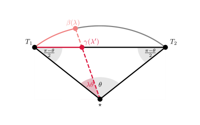
Figure 16: The geodesic triangle in the proof of 4.1. Here, we identify $\Sigma_{\star}$ with the link $\mathbb{L}_{n}$ by Proposition 2.13, and then construct the geodesic $\beta$ by reparametrizing $\gamma$ and projecting back to the link.

Using the law of sines, we obtain

$$\lambda^{\prime}\cdot d(T_{\tau},T)=d\left(T_{\tau},\gamma(\lambda^{\prime})\right)=\frac{\sin(\lambda\cdot\theta)}{\sin\left(\pi-\left(\lambda\theta+\frac{\pi-\theta}{2}\right)\right)}\,.$$

Since, on the other hand,

$$d(T_{\tau},T)=\sqrt{d(\star,T_{\tau})+d(\star,T)-2\cos(\theta)}=\sqrt{\left(2-e^{i\theta}-e^{-i\theta}\right)}=\sqrt{\left(e^{i\frac{\theta}{2}}-e^{-i\frac{\theta}{2}}\right)^{2}}=2\sin\left(\frac{\theta}{2}\right)\,,$$

we have the assertion

$$\lambda^{\prime}=\frac{\sin(\lambda\cdot\theta)}{2\sin\left(\frac{\theta}{2}\right)\sin\left(\frac{\pi+(1-\lambda)\theta}{2}\right)}\,.$$

∎

References

• Allen and Steel (2000) Allen, B. and M. Steel (2000, 09). Subtree transfer operations and their induced metrics on evolutionary trees. Annals of Combinatorics 5.
• Anaya et al. (2020) Anaya, M., O. Anipchenko-Ulaj, A. Ashfaq, J. Chiu, M. Kaiser, M. S. Ohsawa, M. Owen, E. Pavlechko, K. S. John, S. Suleria, et al. (2020). Properties for the Fréchet mean in Billera-Holmes-Vogtmann treespace. Advances in Applied Mathematics 120, 102072.
• Bacák (2014) Bacák, M. (2014). Computing medians and means in Hadamard spaces.
• Barden and Le (2018) Barden, D. M. and H. Le (2018). The logarithm map, its limits and Fréchet means in orthant spaces. Proceedings of the London Mathematical Society 117.
• Baroni et al. (2005) Baroni, M., S. Grünewald, V. Molton, and C. Semple (2005, 08). Bounding the number of hybridisation events for a consistent evolutionary history. Journal of Mathematical Biology 51, 171–182.
• Belinda and K (2010) Belinda, P. and S. G. K (2010, October). Permutation P-values Should Never Be Zero: Calculating Exact P-values When Permutations Are Randomly Drawn. Statistical Applications in Genetics and Molecular Biology 9(1), 1–16.
• Billera et al. (2001) Billera, L. J., S. P. Holmes, and K. Vogtmann (2001). Geometry of the space of phylogenetic trees. Advances in Applied Mathematics 27(4), 733–767.
• Bridson and Häfliger (2011) Bridson, M. and A. Häfliger (2011). Metric Spaces of Non-Positive Curvature. Grundlehren der mathematischen Wissenschaften. Springer Berlin Heidelberg.
• Brown and Owen (2018) Brown, D. G. and M. Owen (2018). Mean and variance of phylogenetic trees.
• Burago et al. (2001) Burago, D., I. Burago, and S. Ivanov (2001). A Course in Metric Geometry. Crm Proceedings & Lecture Notes. American Mathematical Society.
• Durrett (2019) Durrett, R. (2019). Probability: Theory and Examples. Cambridge Series in Statistical and Probabilistic Mathematics. Cambridge University Press.
• Feragen et al. (2013) Feragen, A., M. Owen, J. Petersen, M. Wille, L. Thomsen, A. Dirksen, and de Bruijne M. (2013). Tree-space statistics and approximations for large-scale analysis of anatomical trees. In 23rd biennial International Conference on Information Processing in Medical Imaging (IPMI).
• Garba et al. (2021) Garba, M. K., T. M. Nye, J. Lueg, and S. F. Huckemann (2021). Information geometry for phylogenetic trees. Journal of Mathematical Biology 82(3), 1–39.
• Hein (1990) Hein, J. (1990). Reconstructing evolution of sequences subject to recombination using parsimony. Mathematical Biosciences 98(2), 185–200.
• Holm (1979) Holm, S. (1979). A simple sequentially rejective multiple test procedure. Scandinavian Journal of Statistics 6(2), 65–70.
• Hotz et al. (2013) Hotz, T., S. Skwerer, S. Huckemann, H. Le, J. S. Marron, J. C. Mattingly, E. Miller, J. Nolen, M. Owen, and V. Patrangenaru (2013). Sticky central limit theorems on open books. The Annals of Applied Probability 23(6).
• Huckemann et al. (2015) Huckemann, S., J. C. Mattingly, E. Miller, and J. Nolen (2015). Sticky central limit theorems at isolated hyperbolic planar singularities.
• Kuo et al. (2008) Kuo, C.-H., J. Wares, and J. Kissinger (2008). The apicomplexan whole-genome phylogeny: An analysis of incongruence among gene trees. Molecular Biology and Evolution 25.
• Lammers et al. (2023) Lammers, L., D. T. Van, and S. F. Huckemann (2023). Sticky flavors. arXiv preprint 2311.08846.
• Lammers et al. (2023) Lammers, L., D. T. Van, T. M. W. Nye, and S. F. Huckemann (2023). Types of stickiness in bhv phylogenetic tree spaces and their degree. In F. Nielsen and F. Barbaresco (Eds.), Geometric Science of Information, Cham, pp.  357–365. Springer Nature Switzerland.
• Lauster and Luke (2021) Lauster, F. and D. R. Luke (2021, August). Convergence of proximal splitting algorithms in $\operatorname{CAT}(\kappa)$ spaces and beyond. Fixed Point Theory and Algorithms for Sciences and Engineering 2021(1).
• Lin et al. (2018) Lin, B., A. Monod, and R. Yoshida (2018). Tropical foundations for probability and statistics on phylogenetic tree space. arXiv preprint arXiv:1805.12400.
• Lueg et al. (2024) Lueg, J., M. K. Garba, T. M. Nye, J. Lueg, and S. F. Huckemann (2024). Foundations of wald space for statistics of phylogenetic trees. Journal of the London Mathematical Society 109(5), e12893.
• Maclagan and Sturmfels (2015) Maclagan, D. and B. Sturmfels (2015). Introduction to tropical geometry, Volume 161. American mathematical society Providence, RI.
• Mattingly et al. (2024) Mattingly, J. C., E. Miller, and D. Tran (2024). A central limit theorem for random tangent fields on stratified spaces.
• Miller et al. (2015) Miller, E., M. Owen, and J. S. Provan (2015). Polyhedral computational geometry for averaging metric phylogenetic trees. Advances in Applied Mathematics 68, 51–91.
• Nye (2011) Nye, T. M. W. (2011). Principal components analysis in the space of phylogenetic trees. The Annals of Statistics 39(5), 2716 – 2739.
• Nye et al. (2017) Nye, T. M. W., X. Tang, G. Weyenberg, and R. Yoshida (2017, 09). Principal component analysis and the locus of the Fréchet mean in the space of phylogenetic trees. Biometrika 104(4), 901–922.
• Owen (2008) Owen, M. (2008). Distance computation in the space of phylogenetic trees. PhD thesis.
• Owen (2011) Owen, M. (2011). Computing geodesic distances in tree space. SIAM Journal on Discrete Mathematics 25(4), 1506–1529.
• Owen and Provan (2011) Owen, M. and J. S. Provan (2011). A fast algorithm for computing geodesic distances in tree space. IEEE/ACM Transactions on Computational Biology and Bioinformatics (TCBB) 8(1), 2–13.
• Romano and Lehmann (2005) Romano, J. P. and E. L. Lehmann (2005). Testing statistical hypotheses. Springer, Berlin.
• Skwerer et al. (2014) Skwerer, S., E. Bullitt, S. Huckemann, E. Miller, I. Oguz, M. Owen, V. Patrangenaru, S. Provan, and J. S. Marron (2014). Tree-oriented analysis of brain artery structure. Journal of Mathematical Imaging and Vision 50(1-2), 126–143.
• Skwerer et al. (2018) Skwerer, S., S. Provan, and J. Marron (2018). Relative optimality conditions and algorithms for treespace Fréchet means. SIAM Journal on Optimization 28(2), 959–988.
• Sturm (2003) Sturm, K.-T. (2003, 01). Probability measures on metric spaces of nonpositive curvature. Contemp. Math. 338.
• Sørensen et al. (2023) Sørensen, E. F., R. A. Harris, L. Zhang, M. Raveendran, L. F. K. Kuderna, J. A. Walker, J. M. Storer, M. Kuhlwilm, C. Fontsere, L. Seshadri, C. M. Bergey, A. S. Burrell, J. Bergman, J. E. Phillips-Conroy, F. Shiferaw, K. L. Chiou, I. S. Chuma, J. D. Keyyu, J. Fischer, M.-C. Gingras, S. Salvi, H. Doddapaneni, M. H. Schierup, M. A. Batzer, C. J. Jolly, S. Knauf, D. Zinner, K. K.-H. Farh, T. Marques-Bonet, K. Munch, C. Roos, and J. Rogers (2023). Genome-wide coancestry reveals details of ancient and recent male-driven reticulation in baboons. Science 380(6648), eabn8153.
• Ulmer et al. (2023) Ulmer, S., D. T. Van, and S. F. Huckemann (2023). Exploring uniform finite sample stickiness. In Geometric Science of Information 2023 proceedings, Volume I, pp.  249–356.
• van der Vaart et al. (1996) van der Vaart, A., A. van der Vaart, A. van der Vaart, and J. Wellner (1996). Weak Convergence and Empirical Processes: With Applications to Statistics. Springer Series in Statistics. Springer.
• Weyenberg et al. (2017) Weyenberg, G., R. Yoshida, and D. Howe (2017). Normalizing kernels in the billera-holmes-vogtmann treespace. IEEE/ACM Transactions on Computational Biology and Bioinformatics 14(6), 1359–1365.