Efficient Maximal Frequent Group Enumeration in Temporal Bipartite Graphs

Abstract.

Cohesive subgraph mining is a fundamental problem in bipartite graph analysis. In reality, relationships between two types of entities often occur at some specific timestamps, which can be modeled as a temporal bipartite graph. However, the temporal information is widely neglected by previous studies. Moreover, directly extending the existing models may fail to find some critical groups in temporal bipartite graphs, which appear in a unilateral (i.e., one-layer) form. To fill the gap, in this paper, we propose a novel model, called maximal $\lambda$-frequency group (MFG). Given a temporal bipartite graph $\mathcal{G}=(U,V,\mathcal{E})$, a vertex set $V_{S}\subseteq V$ is an MFG if $i)$ there are no less than $\lambda$ timestamps, at each of which $V_{S}$ can form a $(\tau_{U},\tau_{V})$-biclique with some vertices in $U$ at the corresponding snapshot, and $ii)$ it is maximal. To solve the problem, a filter-and-verification (FilterV) method is proposed based on the Bron-Kerbosch framework, incorporating novel filtering techniques to reduce the search space and array-based strategy to accelerate the frequency and maximality verification. Nevertheless, the cost of frequency verification in each valid candidate set computation and maximality check could limit the scalability of FilterV to larger graphs. Therefore, we further develop a novel verification-free (VFree) approach by leveraging the advanced dynamic counting structure proposed. Theoretically, we prove that VFree can reduce the cost of each valid candidate set computation in FilterV by a factor of $\mathcal{O}(|V|)$. Furthermore, VFree can avoid the explicit maximality verification because of the developed search paradigm. Finally, comprehensive experiments on 15 real-world graphs are conducted to demonstrate the efficiency and effectiveness of the proposed techniques and model.

1. Introduction

Bipartite graphs are widely used to model the complex relationships between two types of entities, e.g., author-paper networks (wang2022towards; wang2020efficient), customer-product networks (lyu2020maximum; yang2021efficient; beutel2013copycatch; kim2022abc; zhou2021butterfly), and patient-disease networks (aziz2021multimorbidity; zhao2019integrating; krishnagopal2020identifying). As a fundamental problem in graph analysis, cohesive subgraph mining is broadly investigated. To analyze the properties of bipartite graphs, many cohesive subgraph models have been proposed, such as $(\alpha,\beta)$-core (DBLP:conf/www/LiuYLQZZ19), bitruss (wang2022towards) and biclique (lyu2020maximum; sun2022maximal; yao2022identifying; DBLP:journals/tkde/SunWWCZL24). Among these models, biclique, which requires every pair of vertices from different vertex sets to be mutually connected, has gained widespread popularity due to its unique features and diverse applications. However, existing models on bipartite graphs primarily focus on static graphs, disregarding the temporal aspect of relationships in real-world applications. For instance, Figure 1 shows a customer-product network. The timestamps on an edge between two vertices indicate when a customer purchased the corresponding product. In a patient-disease network, patients and diseases can be represented by two disjoint vertex sets, and the timestamps on an edge represent when the patient suffered from the disease. The above cases can be modeled as a temporal bipartite graph $\mathcal{G}=(U,V,\mathcal{E})$, where each edge $e\in\mathcal{E}$ can be represented as a tuple $(u,v,t)$, indicating that the interaction between vertex $u\in U$ and vertex $v\in V$ occurs at timestamp $t$ (e.g., (aziz2021multimorbidity; chen2021efficiently)). The bipartite graph with all the edges at timestamp $t$ is called a snapshot of $\mathcal{G}$, denoted by $G_{t}$.

Analyzing the properties of temporal bipartite graphs is essential to reveal more sophisticated semantics. In the literature, many subgraph models are defined for unipartite scenarios. For instance, Li et al. (li2018persistent) propose a $k$-core based model to capture the persistence of a community within the time interval. Qin et al. (qin2019mining) design a clique based model to find the subgraphs periodically occurring in the temporal graphs. Qin et al. (qin2022mining) propose the $(l,\delta)$-maximal bursting core, where each vertex has an average degree no less than $\delta$ during a period of length no less than $l$. Although temporal subgraph search and enumeration problems have been extensively studied on temporal unipartite graphs, the temporal bipartite graph case is still under-explored. Due to the involvement of two distinct types of entities, existing models on temporal unipartite graphs are not suitable for capturing important patterns in temporal bipartite graphs. Only a few recent works consider temporal bipartite graphs, such as $(\alpha,\beta)$-core based persistent community search (li2023persistent) and temporal butterfly counting and enumeration (cai2023efficient). Unfortunately, the aforementioned temporal models are mainly established on interval-based or periodic-based constraints, which fail to capture the real scenarios occurring irregularly at non-consecutive timestamps. Additionally, there is no existing work considering the unilateral (i.e., one-layer) frequency of the occurred group in temporal bipartite graphs, which is an important factor in identifying practical groups. For example, in a temporal customer-product bipartite graph, a group of users who frequently act together (e.g., purchase the same items at different timestamps) may show strong connections. Existing works about temporal subgraph mining are inadequate for the above scenario, highlighting the need to define the exclusive model tailored for temporal bipartite graphs.

To fill the gap, in this paper, we propose a novel model, called Maximal $\lambda$-Frequency Group (MFG), to characterize the unilateral patterns in temporal bipartite graphs. In our model, we leverage biclique to measure the cohesiveness of bipartite subgraphs, due to its diverse applications such as social recommendation (liu2006efficient) and anomaly detection (lyu2020maximum). Specifically, given two size constraints $\tau_{U}$, $\tau_{V}$ and a frequency constraint $\lambda$, a vertex set $V_{S}\subseteq V$ in a temporal bipartite graph $\mathcal{G}=(U,V,\mathcal{E})$ is an MFG if $i)$ there are no less than $\lambda$ timestamps, at each of which $V_{S}$ can form a $(\tau_{U},\tau_{V})$-biclique with some vertices in $U$ in the corresponding snapshot graph, and $ii)$ it is maximal. A $(\tau_{U},\tau_{V})$-biclique $S=(U_{S},$ $V_{S},E_{S})$ is a biclique with $|U_{S}|\geq\tau_{U}$ and $|V_{S}|\geq\tau_{V}$. Note that, an MFG $V_{S}$ is unilateral, i.e., only consists of vertices from $V$. In addition, the vertices in $U$ that form $(\tau_{U},\tau_{V})$-bicliques with $V_{S}$ can be different for different timestamps.

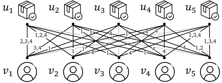
Figure 1. Customer-product temporal bipartite graph (dotted lines denote the edges at $t=5$ for presentation simplicity)

Example 1.0.

Reconsider the temporal customer-product bipartite graph in Figure 1 with $\tau_{U}=2$, $\tau_{V}=2$ and $\lambda=2$. Suppose a company plans to promote a new product to a group of customers with similar interests. Directly extending the static graph model (i.e., biclique) to temporal bipartite graphs may fail to retrieve useful patterns. For instance, if we treat it as a static graph, i.e., ignore the timestamp information, the whole graph itself is a biclique. All five customers will be grouped together and treated equally since they all purchased all the products. If we consider it as a temporal bipartite graph, we still cannot find practical results by applying the frequent $(\tau_{U},\tau_{V})$-biclique model, which is the $(\tau_{U},\tau_{V})$-biclique occurring in at least $\lambda$ snapshots. For the MFG model, $\{v_{2},v_{3},v_{4}\}$ is the returned result, since these customers frequently act together, i.e., it exists in biclique $\{u_{1},u_{2},{v_{2}},$ ${v_{3}},{v_{4}}\}$ at timestamp $t=1$ and in biclique $\{u_{4},u_{5},{v_{2}},{v_{3}},{v_{4}}\}$ at timestamp $t=4$. As discussed before, customers within a group, who frequently act together, are more likely to share similar preferences or behavioral patterns. Identifying these customer-specified communities is crucial to improve the performance of downstream tasks such as product recommendation and enhance customer engagement.

Besides biclique, many other cohesive subgraph models are proposed in the literature for bipartite graph analysis, such as degree-based model $(\alpha,\beta)$-core and butterfly-based model bitruss. All these models have various applications in different domains (DBLP:conf/www/LiuYLQZZ19; wang2022towards). In this paper, we focus more on the strong connections among entities (e.g., co-purchase) in the target layer. Thus, we choose biclique, which is the most cohesive model. Recall the example in Figure 1, if we directly replace the biclique constraint with (2,2)-core in our model, all users $\{v_{1},v_{2},v_{3},v_{4},v_{5}\}$ will be returned as a group.

In this paper, we employ the frequency constraint (i.e., $\lambda$), since frequently appearing patterns are usually worthy of attention and may represent the important concept in the environment (zhang2023discovering; aslay2018mining; yang2016diversified; yang2004complexity; yang2006computational), such as frequent co-purchasing behavior discussed above. Besides, compared with the existing temporal models that mainly focus on interval-based or periodic-based timestamp constraints, our model can better capture the real-world patterns occurring frequently. Moreover, we employ the maximality constraint, since any subset of an MFG with size no less than $\tau_{V}$ is also a $\lambda$-frequency group. Without the maximality constraint, it may generate many redundant results. In this paper, we aim to enumerate all MFGs from a temporal bipartite graph.

In addition to the application of customer analysis mentioned above, MFG can find many other applications in different domains. For instance, a temporal bipartite graph is a suitable data structure to model the data of patients’ diagnostic records, where the vertices correspond to patients (i.e., $U$) and health conditions (i.e., $V$), and the links indicate the presence of a diagnosis at the corresponding timestamp (aziz2021multimorbidity; zhao2019integrating; krishnagopal2020identifying). By mining MFGs from the patient-condition temporal bipartite graph, we can find the combinations of health conditions that frequently and simultaneously appear in multiple patients. The results can provide data support for the study of multimorbidity, facilitating diagnosis and prevention (schafer2014reducing; vetrano2020twelve). In Section LABEL:exp, we present two case studies on real-world datasets to illustrate the effectiveness of our model.

Challenges and our approaches. To the best of our knowledge, we are the first to propose and investigate the maximal $\lambda$-frequency group (MFG) enumeration problem in temporal bipartite graphs. We prove the hardness of counting MFGs. In the literature, maximal biclique enumeration is the most relevant problem to ours (e.g., (abidi2020pivot; chen2022efficient; zhang2014finding; yao2022identifying)). However, the introduction of temporal and unilateral aspects significantly complicates the problem. Naively, we can enumerate all bicliques over each snapshot and post-process the intermediate results. Due to the hardness of the biclique enumeration problem in static bipartite graphs, treating each timestamp separately is time-consuming. Moreover, since the correlation among vertices varies over time, considering temporal and cohesive aspects simultaneously in algorithm design is nontrivial. In previous studies, the Bron-Kerbosch (BK) framework is widely used for biclique enumeration (e.g., (abidi2020pivot; chen2022efficient)). It iteratively adds vertices from the candidate set to expand the current result in a DFS manner for biclique enumeration. By extending the BK framework, in our problem, we need to further check the frequency and maximality constraints for each candidate group. Since MFG focuses on the unilateral vertex set and the number of bicliques in each timestamp is large, it means numerous candidate groups will be generated while only very few of them will belong to the final results. Thus, the huge time cost to apply the naive frequency verification on each candidate group and eliminate the non-maximal results presents a unique challenge for our problem.

To address the challenges, in this paper, we first propose a filter-and-verification (FilterV) approach by leveraging the BK framework. Generally, FilterV maintains a recursive search tree and traverses in a depth-first manner. In each iteration, FilterV iterates over all the candidate vertices (i.e., vertex-oriented search paradigm), verifies the frequency constraint and obtains the valid candidate set. Note that, for each vertex in the valid candidate set, the group composed of it and the current processing set still meets the frequency requirement. If no more vertices can be added to the current processing set to form a new frequent group, FilterV terminates the current search branch and checks the maximality of the vertex set. Since there could be many vertices that cannot be involved in any MFGs, a novel structure $(\tau_{V},\tau_{U},\lambda)$-core is first designed to reduce the search space. Then, a filter strategy is proposed to first efficiently prune the candidate set before the examination, which can reduce the unnecessary call of frequency verification. To further accelerate the frequency verification of a given vertex set, we present an elaborate array-based verification strategy. The frequency check method is also employed to accelerate the maximality verification by avoiding the numerous set comparisons.

Even though FilterV can remarkably accelerate the MFG enumeration procedure, we need to compute the valid candidate set for each current processing result during the search. The overall cost significantly increases with the size of candidate set and the workload of maximality verification, which may hinder its scalability to larger graphs. As shown in Table LABEL:tab:timeofgcs, whose details can be found in Section LABEL:sec:method2, the components of the valid candidate set computation and maximality verification take up a majority of the overall execution time. Therefore, if we can reduce or even avoid the cost of frequency and maximality verification to some extent, the overall performance can be significantly improved. Motivated by this, we further develop a novel verification-free (VFree) approach. Instead of iterating over vertices during the candidate set computation and maximality verification, we develop a timestamp-oriented search paradigm. That is, VFree iterates through the timestamps to obtain the valid candidate set using the advanced dynamic counting structures proposed, where the unpromising timestamp can be skipped and common neighbor information can be carried forward in the subsequent search process. Theoretically, we prove that VFree can significantly reduce each valid candidate set computation cost in FilterV by a factor of $\mathcal{O}(|V|)$. Additionally, by integrating the developed search paradigm and dynamic counting techniques, VFree can avoid explicit maximality verification.

Contributions. The main contributions of the paper are summarized as follows.

• To capture the properties of temporal bipartite graphs, we conduct the first research to propose and investigate the maximal $\lambda$-frequency group enumeration problem. (Section 2)

• To solve the problem, we introduce a filter-and-verification framework. Novel $(\tau_{V},\tau_{U},\lambda)$-core structure and candidate filtering rule are developed to shrink the search space. Advanced array-based method is proposed to accelerate the computation of valid candidate set and maximality verification. (Section 3)

• To overcome the frequency verification cost and scale for larger networks, we further develop a verification-free framework by leveraging the dynamic counting structure proposed. The framework can also avoid the explicit verification of maximality based on the propounded search paradigm. (Section LABEL:sec:method2)

• Extensive experiments are conducted on 15 real-world graphs to demonstrate the performance of proposed techniques and model. Compared with the baseline, the optimized method can achieve up to three orders of magnitude speedup. (Section LABEL:exp)

2. Preliminary and Problem Definition

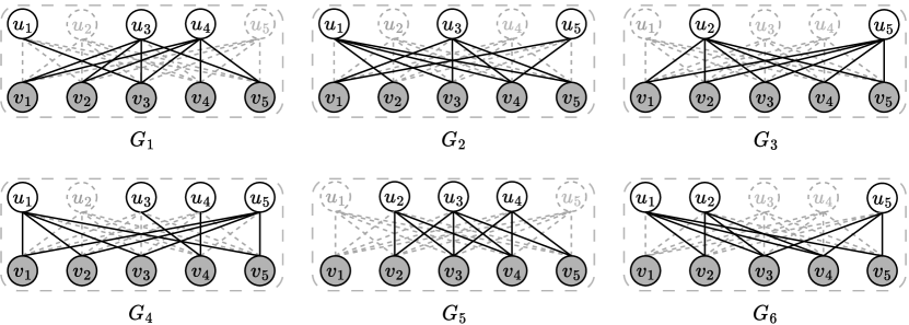
Figure 2. A temporal bipartite graph $\mathcal{G}$ with six timestamps ($G_{1}$-$G_{6}$ are the corresponding snapshots and solid lines denote the edges in each snapshot)

2.1. Preliminary

Let $\mathcal{G}=(U,V,\mathcal{E})$ denote an undirected temporal bipartite graph, where $U$ and $V$ are two disjoint vertex sets, i.e., $U\cap V=\emptyset$, and $\mathcal{E}$ is the set of temporal edges. $(u,v,t)$ denotes a temporal edge between $u\in U$ and $v\in V$, where $t$ is the interaction timestamp between $u$ and $v$. Without loss of generality, we use $\mathcal{T}=\{t_{1},t_{2},\dots,t_{|\mathcal{T}|}\}$ to represent the set of timestamps, i.e., $\mathcal{T}=\{t|(u,v,t)\in\mathcal{E}\}$. Given a temporal bipartite graph $\mathcal{G}$, its corresponding static bipartite graph, i.e., by ignoring all the timestamps on edges, is denoted by $G=(U,V,E)$, where $E=\{(u,v)|(u,v,t)\in\mathcal{E}\}$. We can extract a series of snapshots $\{G_{1},G_{2},\dots,G_{\mathcal{|T|}}\}$ from $\mathcal{G}$ based on the timestamps. Specifically, given a timestamp $t\in\mathcal{T}$, its corresponding snapshot is a bipartite graph $G_{t}=(U_{t},V_{t},E_{t})$, where $U_{t}=\{u|(u,v,t)\in\mathcal{E}\}$, $V_{t}=\{v|(u,v,t)\in\mathcal{E}\}$, and $E_{t}=\{(u,v)|(u,v,t)\in\mathcal{E}\}$.

Definition 2.0 (Structural neighbor (s-neighbor)).

Given a vertex $u\in\mathcal{G}$, the s-neighbor set of $u$ is the set of vertices connected to $u$ in $G$, denoted by ${N(u,{G})}$, i.e., ${N(u,{G})}=\{v|(u,v)\in E\}$. ${d(u,{G})}$ denotes its structural degree (s-degree), i.e., ${d(u,{G})}$ $=|{N(u,{G})}|$.

Definition 2.0 (Momentary neighbor (m-neighbor)).

Given a vertex $u\in\mathcal{G}$ and a timestamp $t\in\mathcal{T}$, the m-neighbor set of $u$ at $t$ is the set of vertices connected to $u$ in $G_{t}$, denoted by ${\Gamma(u,t)}$, i.e., ${\Gamma(u,t)}=\{v|(u,v)\in E_{t}\}$. We use ${\delta(u,t)}$ to denote its momentary degree (m-degree) at $t$, i.e., ${\delta(u,t)}=|{\Gamma(u,t)}|$.

Example 2.0.

Figure 2 shows a temporal bipartite graph with six snapshots $G_{1}$ to $G_{6}$. The s-neighbors of $u_{1}$ are $\{v_{1},v_{2},v_{3},v_{4},v_{5}\}$ and the s-degree ${d(u_{1},{G})}$ is 5. The m-neighbor of $u_{1}$ at $t=1$ is $\{v_{3}\}$ and the corresponding m-degree ${\delta(u_{1},1)}$ is 1.

Given a static bipartite graph $G=(U,V,E)$, a biclique $S=(U_{S},V_{S},E_{S})$ is a complete subgraph of $G$, where $U_{S}\subseteq U$, $V_{S}\subseteq V$, and for each pair of vertices $u\in U_{S}$ and $v\in V_{S}$, we have $(u,v)\in E_{S}$.

Definition 2.0 ($(\tau_{U},\tau_{V})$-biclique).

Given a static bipartite graph $G$ and two positive integers $\tau_{U}$ and $\tau_{V}$, a $(\tau_{U},\tau_{V})$-biclique $S=(U_{S},$ $V_{S},E_{S})$ is a biclique of $G$ with $|U_{S}|\geq\tau_{U}$ and $|V_{S}|\geq\tau_{V}$.

2.2. Problem Definition

In this paper, we aim to retrieve the frequent vertex set in unilateral layer, e.g., the customer set in Figure 1. For presentation simplicity, we assume the frequent vertex set is from $V$. Before introducing the $\lambda$-frequency group, we first define the support timestamp for the unilateral vertex set below.

Definition 2.0 (Support timestamp).

Given a temporal bipartite graph $\mathcal{G}=(U,V,\mathcal{E})$, a subset $V_{S}\subseteq V$, a snapshot $G_{t}=(U_{t},V_{t},E_{t})$ of the timestamp $t\in\mathcal{T}$, and two positive integers $\tau_{U}$, $\tau_{V}$, we say $t$ is a support timestamp of $V_{S}$, if $i)$ $V_{S}\subseteq V_{t}$, and $ii)$ $V_{S}$ can form a $(\tau_{U},\tau_{V})$-biclique with a subset of vertices in $U_{t}$, i.e., $V_{S}$ is included in a $(\tau_{U},\tau_{V})$-biclique of $G_{t}$.

Definition 2.0 ($\lambda$-frequency group).

Given a temporal bipartite graph $\mathcal{G}=(U,V,\mathcal{E})$, and three positive integers $\tau_{U}$, $\tau_{V}$ and $\lambda$, a $\lambda$-frequency group is a subset of vertices $V_{S}\subseteq V$ where there are at least $\lambda$ support timestamps in $\mathcal{T}$ for $V_{S}$.

Definition 2.0 (Maximal $\lambda$-frequency group (MFG)).

Given a temporal bipartite graph $\mathcal{G}=(U,V,\mathcal{E})$ and three positive integers $\tau_{U}$, $\tau_{V}$ and $\lambda$, a $\lambda$-frequency group $V_{S}$ is maximal if there is no other $\lambda$-frequency group $V^{\prime}_{S}$ that is a superset of $V_{S}$.

Problem definition. Given a temporal bipartite graph $\mathcal{G}$ and three positive integers $\tau_{U}$, $\tau_{V}$ and $\lambda$, in this paper, we aim to find all the maximal $\lambda$-frequency groups (MFGs) in $\mathcal{G}$.

Example 2.0.

Considering the temporal bipartite graph shown in Figure 2, suppose $\tau_{U}=\tau_{V}=2$ and $\lambda=3$. There are three MFGs in the graph, i.e., $V_{S1}=\{v_{1},v_{2},v_{3},v_{5}\}$ with 3 support timestamps $\{t_{1},t_{3},t_{4}\}$, $V_{S2}=\{v_{2},v_{3},v_{4}\}$ with 3 support timestamps $\{t_{3},t_{5},t_{6}\}$ and $V_{S3}=\{v_{3},v_{4},v_{5}\}$ with 4 support timestamps $\{t_{2},t_{3},t_{5},t_{6}\}$.

Problem properties. Based on the definition of MFG, Lemmas 2.9 and 2.10 can be immediately obtained. The proofs are omitted. Then, we show the hardness of our problem in Theorem 2.11.

Lemma 2.0 (Structural property).

Given a temporal bipartite graph $\mathcal{G}=(U,V,\mathcal{E})$ and three positive integers $\tau_{U}$, $\tau_{V}$ and $\lambda$, any MFG $V_{S}\subseteq V$ must be contained in a maximal $(\tau_{U},\tau_{V})$-biclique of the static bipartite graph $G$ of $\mathcal{G}$.

Lemma 2.0 (Antimonotone property).

Given a vertex set $V_{S}\subseteq V$, $i)$ if $V_{S}$ satisfies the frequency constraint, any subset of $V_{S}$ also satisfies the constraint; $ii)$ if $V_{S}$ does not meet the frequency constraint, any superset of $V_{S}$ is not frequent.

Theorem 2.11.

The problem of counting all MFGs is #P-complete.

Proof.

We reduce a well-known #P-complete problem of counting maximal $\sigma$-frequency itemsets (yang2004complexity; yang2006computational) to the MFGs counting problem with $\tau_{U}\geq 1$, $\tau_{V}\geq 1$ and $\lambda=\sigma$. Let $X=\{x_{1},x_{2},\dots,x_{n}\}$ be a set of items. Given a database $\mathcal{D}$ consisting of $|\mathcal{T}|$ transactions, i.e., $\mathcal{D}=\{d_{1},d_{2},\dots,d_{|\mathcal{T}|}\}$. Each transaction $d_{i}$ comprises several items in $X$, i.e., $d_{i}\subseteq X$. The maximal $\sigma$-frequency itemsets problem is to enumerate all subsets $\{I_{1},I_{2},\dots,I_{k},\dots\}$, where each subset $I_{k}$ satisfies that $i)$ $I_{k}\subseteq X$, $ii)$ $|\{d_{i}\in\mathcal{D}|I_{k}\subseteq d_{i}\}|\geq\sigma$ and $iii)$ any superset of $I_{k}$ does not meet $i)$ and $ii)$.

We construct an instance of a temporal bipartite graph $\mathcal{G}=(U,V,\mathcal{E})$ from $X$ and $\mathcal{D}$ to prove the hardness. First, we generate $\tau_{U}$ vertices to form set $U$. Second, for each item $x_{j}\in X$, a vertex $v_{j}$ is correspondingly created to form set $V$, i.e., $|V|=|X|$. Let $V_{i}\subseteq V$ be the set of vertices, where each vertex $v_{j}$ corresponds to each item $x_{j}$ in the transaction $d_{i}\in\mathcal{D}$, $|V_{i}|=|d_{i}|$. Third, for each transaction $d_{i}$, we generate a timestamp $t_{i}$ such that each $v_{j}\in V_{i}$ connects to all vertices in $U$ at this timestamp. Then, there will be $|\mathcal{T}|$ timestamps in $\mathcal{G}$, and $(U,V_{i})$ is the only one biclique at the timestamp $t_{i}$.

We then show that this transformation of $X$ and $\mathcal{D}$ into $\mathcal{G}$ is a reduction. Suppose $\{I_{1},I_{2},\dots,I_{k},\dots\}$ is the set of all the maximal $\sigma$-frequency itemsets w.r.t $\mathcal{D}$ in $X$. We claim that the corresponding vertex sets $\{V_{1},V_{2},\dots,V_{k},\dots\}$ is the set of all MFGs in $\mathcal{G}$. Take the vertex set $V_{k}$ as an example. We first prove that $V_{k}$ is a $\lambda$-frequency group. According to the above construction, $V_{k}$ can form a biclique with $U$ at no less than $\lambda$ timestamps, since $I_{k}$ must be the subset of at least $\sigma$ transactions in $\mathcal{D}$ and $\lambda=\sigma$. Second, we prove the maximality of the $V_{k}$. Suppose to the contrary that $V_{k}$ is not maximal (i.e., there is a vertex $v_{j}$ that can join $V_{k}$ to form a new MFG), $I_{k}$ is not maximal, since $I_{k}\cup\{x_{j}\}$ will be a $\sigma$-frequency itemset. This contradicts the condition that $I_{k}$ is maximal. Third, if there exists an MFG $V_{z}$ that is not included in $\{V_{1},V_{2},\dots,V_{k},\dots\}$, there must exist the other itemset $I_{z}\notin\{I_{1},I_{2},\dots,I_{k},\dots\}$ that is $\sigma$-frequency. Therefore, $\{V_{1},V_{2},\dots,V_{k},\dots\}$ is the complete set of all MFGs in $\mathcal{G}$. Conversely, assume that $\{V^{\prime}_{1},V^{\prime}_{2},\dots,V^{\prime}_{k},\dots\}$ are the set of all MFGs in $\mathcal{G}$. Based on the definition of MFG and the above construction, the one-to-one correspondence between the maximal $\sigma$-frequency itemsets of $\mathcal{D}$ and the MFG in $\mathcal{G}$ is established. Therefore, if we count the number of all $\sigma$-frequency itemsets of $\mathcal{D}$, we can obtain the number of all MFGs. The reduction is realized. Therefore, the problem of counting the number of MFGs is #P-complete. ∎

Note that, our enumeration problem is at least as hard as the counting problem, because if we can enumerate all the results, then we can easily count the total number.

3. filter-and-verification approach

Input : $\mathcal{G}=(U,V,\mathcal{E})$: a temporal bipartite graph,

$\tau_{U}$, $\tau_{V}$: size constraints, $\lambda$: frequency constraint

Output : $\mathcal{R}$: all the MFGs

AlgoLine0.1

$\mathcal{G}\leftarrow$ GFCore$(\mathcal{G},\tau_{U},\tau_{V},\lambda)$;  /* graph filter: Algorithm 2 */AlgoLine0.2

$\mathcal{R}\leftarrow\emptyset$;AlgoLine0.3

EnumMFG$(U,\emptyset,V)$;AlgoLine0.4

AlgoLine0.5

Procedure EnumMFG$(U_{S},V_{S},C_{V})$AlgoLine0.6

$C_{V}\leftarrow$ filter candidate set $C_{V}$;  /* candidate filter: Lemma 3.4 */AlgoLine0.7

$C^{*}_{V}\leftarrow\emptyset$;  /* compute valid candidate set */AlgoLine0.8

for each $v\in C_{V}$ do  if CheckFRE($U_{S}\cap{N(v,{G})},V_{S}\cup\{v\},\lambda$) then /* Algorithm 3 */  $C^{*}_{V}\leftarrow C^{*}_{V}\cup\{v\}$; AlgoLine0.9

    if $|U_{S}|<\tau_{U}$ $\lor$ $|V_{S}|+|C^{*}_{V}|<\tau_{V}$ then  return; AlgoLine0.10

  if $C^{*}_{V}=\emptyset$ then  Check the maximality for $V_{S}$;  /* Section LABEL:subsec:mal */ AlgoLine0.11

AlgoLine0.12

if $V_{S}$ is maximal then $\mathcal{R}\leftarrow\mathcal{R}\cup\{V_{S}\}$;AlgoLine0.13

  for each $v\in C^{*}_{V}$ do  $C^{*}_{V}\leftarrow C^{*}_{V}\backslash\{v\}$; AlgoLine0.14

EnumMFG$(U_{S}\cap N(v,G),V_{S}\cup\{v\},C^{*}_{V})$;AlgoLine0.15

  AlgoLine0.16

Algorithm 1 Filter-and-Verification (FilterV)

16

16

16

16

16

16

16

16

16

16

16

16

16

16

16

16

In the literature, the closest problem to ours is the maximal biclique enumeration problem (e.g., (abidi2020pivot; chen2022efficient; zhang2014finding)), where most studies are based on the Bron-Kerbosch (BK) framework. It maintains a recursion search tree and traverses in a depth-first manner.

Baseline method. Motivated by Lemmas 2.9 and 2.10, a reasonable approach for our problem is to employ the BK framework by jointly considering the frequency and maximality constraints. Specifically, we operate on three dynamically changing vertex sets $(U_{S},V_{S},C_{V})$. $V_{S}$ is the current result. $U_{S}$ is the common s-neighbors of all the vertices in $V_{S}$. $C_{V}$ is the candidate set. In each iteration, we select a vertex from the candidate set $C_{V}$ to expand $V_{S}$, and update the corresponding $U_{S}$. If $V_{S}$ satisfies the frequency constraint, we continue to expand it. If no other vertex can be added into $V_{S}$ to form a new frequent group, we terminate the current search branch and check the maximality of $V_{S}$ by comparing it with the existing found results. After enumerating through each search branch, all the MFGs are returned. This algorithm is referred to as BK-ALG.

Limitations. Although BK-ALG can correctly return all the MFGs for a given temporal bipartite graph, we find that directly extending the BK framework is inefficient due to the following two drawbacks. The first drawback is the huge search space. The search space of BK-ALG is the whole graph $\mathcal{G}$, and it needs to iterate through all the vertices in $C_{V}$ in each branch, which may involve many unpromising vertices that cannot exist in any MFG. The second drawback is the cumbersome frequency constraint check. Similar to biclique enumeration in static graphs, in BK-ALG, $C_{V}$ maintains the candidate vertices and we need to ensure the frequency constraint during the search, which is computationally expensive.

To address these limitations, in this section, we propose a novel filter-and-verification (FilterV) algorithm. In the following, we first introduce the search framework of FilterV (Section 3.1). For drawback 1, we develop novel graph and candidate set filtering techniques to dramatically shrink search space (Section 3.2). For drawback 2, an advanced array-based algorithm is presented to facilitate the frequency (Section 3.3) and maximality (Section LABEL:subsec:mal) verification.

3.1. Framework Overview

Hereafter we present an overview of our filter-and-verification (FilterV) framework. We call each search branch that fails to find an MFG an invalid branch. Recall the search branch $(U_{S},V_{S},C_{V})$. To reduce even avoid the search cost on invalid search branches, instead of directly adding each candidate vertex from $C_{V}$ into $V_{S}$, we first perform a verification procedure on $C_{V}$ to generate the valid candidate set $C^{*}_{V}\subseteq C_{V}$ for $V_{S}$. That is, in subsequent branches, the new set obtained by adding any candidate vertex from $C_{V}^{*}$ to the current processing set $V_{S}$ still can meet the frequency requirement.

FilterV framework. Motivated by the above idea, the pseudocode of FilterV framework is presented in Algorithm 1. It first applies the graph filtering technique (Algorithm 2 in Section 3.2) to shrink the given temporal bipartite graph. In the following, FilterV invokes the procedure EnumMFG to enumerate all the MFGs. Similar as the BK method, EnumMFG maintains three sets $U_{S}$, $V_{S}$ and $C_{V}$, which are initialized as $U$, $\emptyset$ and $V$. In EnumMFG, we first try to filter the candidate set $C_{V}$ (line 5) and then compute the valid candidate set $C^{*}_{V}$ for $V_{S}$ (lines 7-9). The branch is terminated if it violates the $(\tau_{U},\tau_{V})$-biclique size constraints. We check the maximality of $V_{S}$ when the valid candidate set is empty (lines 12-14). If $C^{*}_{V}$ is not empty, we process each vertex $v\in C^{*}_{V}$ to expand $V_{S}$, and continue search on the updated $V_{S}$ and $U_{S}$ (lines 15-17).

Discussion. To compute the valid candidate set $C^{*}_{V}$ for $V_{S}$ in lines 7-9, we need to check the frequency of each vertex set $V_{S}\cup\{v\}$ for $v\in C_{V}$. Given the vertex set $V_{S}$ and the checking vertex $v\in C_{V}$, a naive method to check the frequency of $V_{S}\cup\{v\}$ is to compute the common m-neighbors of $V_{S}\cup\{v\}$ at each timestamp. Specifically, for each timestamp $t\in\mathcal{T}$, we check whether there exists no less than $\tau_{U}$ common m-neighbors of all the vertices in $V_{S}\cup\{v\}$. If it satisfies the constraint, $t$ can contribute to the frequency for $V_{S}\cup\{v\}$. If the number of such timestamps for $V_{S}\cup\{v\}$ is no less than $\lambda$, $v$ is the valid candidate vertex for $V_{S}$ and it can be added into $C^{*}_{V}$. After checking all vertices in $C_{V}$, we can return $C^{*}_{V}$. Due to the large scale of candidate vertices and the inefficiency of the naive frequency checking method, the above process is very time-consuming. To speed up the computation of the valid candidate set, we designed novel filtering strategies and efficient verification techniques.

3.2. Filtering Rules

Graph filter. Given a temporal bipartite graph $\mathcal{G}$, many unpromising vertices cannot exist in any MFGs. Therefore, we propose a novel graph structure to filter the search space. Before presenting the details, we first introduce the concept of $(\alpha,\beta)$-core (DBLP:conf/www/LiuYLQZZ19).

Definition 3.0 ($(\alpha,\beta)$-core).

Given a static bipartite graph $G$ and two positive integers $\alpha$ and $\beta$, the subgraph $S=(U_{S},V_{S},E_{S})$ is the $(\alpha,\beta)$-core of $G$, denoted by $\textsf{Core}(G)$, if it satisfies: $i)$ the degree of each vertex in $U_{S}$ is at least $\alpha$ and the degree of each vertex in $V_{S}$ is at least $\beta$ in $S$, and $ii)$ any supergraph of $S$ cannot satisfy $i)$.

To compute the $(\alpha,\beta)$-core, we can iteratively remove the vertices that violate the degree constraint with time complexity $\mathcal{O}(|E|)$. Based on the definition and properties of MFG, we can obtain that every vertex of MFG must be contained in the temporal bipartite graph $\{\textsf{Core}(G_{1}),\textsf{Core}(G_{2}),\dots,\textsf{Core}(G_{|\mathcal{T}|})\}$. To further model the frequency property of the vertex, we present a new frequent cohesive subgraph model, called $(\tau_{V},\tau_{U},\lambda)$-core, which will be applied to prune unpromising vertices before enumerating all the MFGs.

Definition 3.0 ($(\tau_{V},\tau_{U},\lambda)$-core).

Given a temporal bipartite graph $\mathcal{G}$ and three positive integers $\tau_{U}$, $\tau_{V}$ and $\lambda$, the induced subgraph $(U_{S},V_{S},\mathcal{E}_{S})$ of $\mathcal{G}$ is the $(\tau_{V},\tau_{U},\lambda)$-core if it meets the following conditions: $i)$ each vertex $u\in U_{S}$ can be included in the $(\tau_{V},\tau_{U})$-core of at least one snapshot, $ii)$ each vertex $v\in V_{S}$ can be included in the $(\tau_{V},\tau_{U})$-core of at least $\lambda$ snapshots, and $iii)$ there is no supergraph of $(U_{S},V_{S},\mathcal{E}_{S})$ that satisfies $i)$ and $ii)$.

Note that, in $(\tau_{U},\tau_{V})$-biclique, $\tau_{U}$ and $\tau_{V}$ restrict the number of vertices in $U$ and $V$. But, in Definition 3.2, the parameters restrict the number of neighbors, so the order is changed. Based on the analysis, we can directly obtain the connection between the $(\tau_{V},\tau_{U},\lambda)$-core and the proposed MFG model, detailed in the following lemma.

Lemma 3.0.

Given a temporal bipartite graph $\mathcal{G}=(U,V,\mathcal{E})$ and three positive integers $\tau_{U}$, $\tau_{V}$ and $\lambda$, if a subset $V_{S}\subseteq V$ is an MFG, then $V_{S}$ must be contained in the $(\tau_{V},\tau_{U},\lambda)$-core of $\mathcal{G}$.

Input : $\mathcal{G}=(U,V,\mathcal{E})$: a temporal bipartite graph,

$\tau_{U}$, $\tau_{V}$: size constraints, $\lambda$: frequency constraint

Output : $(\tau_{V},\tau_{U},\lambda)$-core of $\mathcal{G}$

AlgoLine0.1

for each $w\in\mathcal{G}$ do $s[w]=0$;AlgoLine0.2

for each $t\in\mathcal{T}$ do  for each $w\in\mathcal{G}$ do  if $w\in U\land\delta(w,t)>0$ then $s[w]++$; AlgoLine0.3

if $w\in V\land\delta(w,t)>0$ then $s[w]++$;AlgoLine0.4

    for each $t\in\mathcal{T}$ do  for each $w\in\mathcal{G}$ do  if $w\in U\land 0<\delta(w,t)<\tau_{V}$ then  CorePrune$(w,t)$; AlgoLine0.5

  if $w\in V\land(0<\delta(w,t)<\tau_{U}\lor 0<s[w]<\lambda)$ then  CorePrune$(w,t)$; AlgoLine0.6

      for each $t\in\mathcal{T}$ do  for each $w\in\mathcal{G}$ do  if $\delta(w,t)=0$ then $G_{t}\leftarrow G_{t}\backslash\{w\}$; AlgoLine0.7

    return $\{G_{1},G_{2},\dots,G_{|\mathcal{T}|}\}$;AlgoLine0.8

AlgoLine0.9

Procedure CorePrune$(w,t)$AlgoLine0.10

$\delta(w,t)=0$;AlgoLine0.11

for each $x\in\Gamma(w,t)$ do  if $\delta(x,t)>0$ then  $\delta(x,t)=\delta(x,t)-1$; AlgoLine0.12

if $(x\in U\land\delta(x,t)<\tau_{V})\lor(x\in V\land\delta(x,t)<\tau_{U})$ then  CorePrune$(x,t)$; AlgoLine0.13

      if $s[w]>0$ then  $s[w]=s[w]-1$; AlgoLine0.14

if $(w\in U\land s[w]<1)\lor(w\in V\land s[w]<\lambda)$ then  $s[w]=0$; AlgoLine0.15

for each $t\in\mathcal{T}$ do  if $\delta(w,t)>0$ then  CorePrune$(w,t)$; AlgoLine0.16

       

Algorithm 2 GFCore$(\mathcal{G},\tau_{U},\tau_{V},\lambda)$

16

16

16

16

16

16

16

16

16

16

16

16

16

16

16

16

To derive the $(\tau_{V},\tau_{U},\lambda)$-core, we can iteratively delete the vertex that violates the degree constraint or the frequency constraint. Since the deletion of one vertex may cause its neighbors to violate the constraints in cascade, we can iteratively prune the graph until all the remaining vertices in $\mathcal{G}$ meet the constraints. Details of computing $(\tau_{V},\tau_{U},\lambda)$-core are shown in Algorithm 2. At first, we use $s[w]$ to count the number of timestamps when the vertex $w$ has enough m-neighbors (lines 1-5). Then we process all the vertices at each timestamp in lines 6-11. Specifically, for each vertex $w$, if $s[w]$ violates the frequency constraint or the m-degree constraint at $t$, we remove this vertex at $t$ and invoke the procedure CorePrune to update the graph. Details of CorePrune are shown in lines 16-29. For the processing vertex $w$ at timestamp $t$ in line 16, we set $\delta(w,t)$ as 0 and traverse all m-neighbors of $w$ at $t$, i.e., $\Gamma(w,t)$. For each vertex $x\in\Gamma(w,t)$, we first check its m-degree. If it is larger than 0, we reduce its m-degree by 1 (lines 19-20). Then, if $x$ violates the m-neighbor constraint at $t$, we invoke CorePrune for $(x,t)$ in lines 21-22. For the vertex $w$ with $s[w]>0$, we need to update $s[w]$ for it in lines 23-29. We first reduce $s[w]$ by 1. If $s[w]$ violates the constraint, we set $s[w]$ as 0 and invoke CorePrune for $w$ at all timestamps (lines 25-29). After updating the graph, we remove all unsatisfied vertices at each snapshot (lines 12-14). Finally, we return all the updated snapshots as the reduced graph in line 15. Similar as $(\alpha,\beta)$-core, the time complexity is bounded by $\mathcal{O}(|\mathcal{E}|)$.

Candidate set filter. Recall the search branch with processed vertex sets $(U_{S},V_{S},C_{V})$, where we iteratively add one vertex from $C_{V}$ into $V_{S}$ and check its frequency. If we can efficiently skip a batch of vertices in $C_{V}$ without compromising any results, we can reduce many unnecessary calls of frequency check. To achieve this, we propose the following rule to quickly filter the candidate vertex set.

Lemma 3.0 (Candidate set filtering rule).

Given a temporal bipartite graph $\mathcal{G}=(U,V,\mathcal{E})$ and $v\in V$, we use ${T(v)}$ to denote the set of timestamps when $v$ has more than $\tau_{U}$ m-neighbors, i.e., ${T(v)}=\{t|t\in$ $\mathcal{T}$ $\land$ $\delta(v,t)\geq\tau_{U}\}$. Then, for the current processing vertex sets $V_{S}$, we can skip a candidate vertex $v^{\prime}\in C_{V}$, if $|\cap_{v\in V_{S}\cup\{v^{\prime}\}}{T}(v)|<\lambda$.

Proof.

If $|\cap_{v\in V_{S}\cup\{v^{\prime}\}}{T}(v)|<\lambda$, it means that there exists less than $\lambda$ timestamps, when the number of common m-neighbors of $V_{S}\cup\{v^{\prime}\}$ is no less than $\tau_{U}$. Therefore, $V_{S}\cup\{v^{\prime}\}$ is not frequent and we can prune $v^{\prime}$ from $C_{V}$, and the lemma holds. ∎

3.3. Frequency Verification

Recall the computation of the valid candidate set $C^{*}_{V}$ for $V_{S}$, whose main cost is the frequency verification for all the vertex sets $V_{S}\cup\{v\}$, where $v\in C_{V}$. In addition, as discussed before, the naive frequency verification method is very time-consuming. Therefore, reducing the cost of frequency verification is crucial for optimizing the performance of algorithm. Motivated by this, in this section, we design a novel array-based structure to speed up the processing. The detailed method is presented in Algorithm 3.

Input : $U_{S}$: the common s-neighbors of all the vertices in $V_{S}$,

$V_{S}$: the checking vertex set, $\lambda$: frequency constraint

Output : frequency verification result true/false

AlgoLine0.1

$\lambda^{\prime}=0$;AlgoLine0.2

for each $t\in\mathcal{T}$ do UA$[t]$ = 0;  /* Update Array */AlgoLine0.3

AlgoLine0.4

for each $u\in U_{S}$ do  for each $t\in\mathcal{T}$ do RA$[t]$ = 0;  /* Reborn Array */ AlgoLine0.5

AlgoLine0.6

for each $v\in N(u,G)\land v\in V_{S}$ do  for each $t\in\mathcal{T}_{(u,v)}$ do  RA$[t]++$;  /* count $u$’s m-neighbors in $V_{S}$ at $t$ */ AlgoLine0.7

    for each $t\in\mathcal{T}$ do  if RA$[t]$$=|V_{S}|$ then  UA$[t]++$;  /* count common m-neighbors of $V_{S}$ at $t$ */ AlgoLine0.8

   

Algorithm 3 CheckFRE$(U_{S},V_{S},\lambda)$