Uncertainty-Guided Optimization on
Large Language Model Search Trees

Abstract

Beam search is a standard tree search algorithm when it comes to finding sequences of maximum likelihood, for example, in the decoding processes of large language models. However, it is myopic since it does not take the whole path from the root to a leaf into account. Moreover, it is agnostic to prior knowledge available about the process: For example, it does not consider that the objective being maximized is a likelihood and thereby has specific properties, like being bound in the unit interval. Taking a probabilistic approach, we define a prior belief over the LLMs’ transition probabilities and obtain a posterior belief over the most promising paths in each iteration. These beliefs are helpful to define a non-myopic Bayesian-optimization-like acquisition function that allows for a more data-efficient exploration scheme than standard beam search. We discuss how to select the prior and demonstrate in on- and off-model experiments with recent large language models, including Llama-2-7b, that our method achieves higher efficiency than beam search: Our method achieves the same or a higher likelihood while expanding fewer nodes than beam search.

Code: https://github.com/juliagrosse/ults

1 Introduction

Beam search [18] is an optimization algorithm commonly applied to graph-, and in particular tree-structured problems. The number of possible paths that need to be considered in such settings typically grows exponentially, often exceeding the computational budget required to examine them all. This inevitably leads to computational uncertainty [12]: an uncertainty that could be fully resolved if enough compute was available to examine all paths, but in practice is present due to the limited resources. The standard beam search algorithm, while ubiquitous—e.g., in natural language processing for generating sentences under a large language model (LLM) and especially common in summarization and translation tasks [34, 46, 44, 37]—completely ignores this uncertainty.

We posit that quantifying this uncertainty can be beneficial to ensure better explorations on LLMs’ search trees. To this end, we incorporate computational uncertainty into the search process to guide it in a non-myopic fashion (i.e., accounting for the belief about future nodes) and importantly, in a more data-efficient manner, akin to Bayesian optimization methods [BO, 21, 28, 6]. BO methods are recognized for their data efficiency, not merely because they quantify uncertainty, but because they exploit the structural characteristics within that uncertainty. E.g., in continuous optimization problems, prior knowledge, such as the smoothness of a function, is often available through Gaussian processes [30] or (Bayesian) neural networks [14, 19, 20].

Figure 1: The intuition of our method—faded color represents unexplored subtrees. We sequentially expand a node of the LLM search tree based on the posterior belief. The latter is obtained by conditioning the unknown (the optimal total likelihood $\max c_{x_{0}\to x_{i}\to x_{n}}$ from the root $\boldsymbol{x}_{0}$ to a leaf $x_{n}$ when continuing down a particular node $x_{i}$) on the current observations (the total likelihood so far $c_{\boldsymbol{x}_{0}\to x_{i}}$ up until that node). This belief is induced by a simple prior belief on the LLM softmax probabilities $\boldsymbol{c}$. The samples of the posterior belief are used to score the unexplored subtrees.

Unlike standard BO, however, beam search performs discrete optimization—its search space is a tree. Moreover, commonly, the values or rewards associated with each node are probabilities, bounded between $0$ and $1$. Hence, uncertainty quantification here is not as well-studied as in standard BO. We will therefore assume that rewards at a node of the search tree are components of a discrete distribution. The characteristic property we aim to exploit is the concentration strength: whether the Categorical distributions are all highly concentrated at a few realistic options, or if some of them are nearly uniform, making any individual option drastically less likely to be the optimal one. Intuitively, one would expect this to have a strong influence on the number of paths that need to be considered. For instance, when the distribution is concentrated, it is less likely that other paths will overtake later on and one can be more greedy. Meanwhile, when the distribution has high entropy, the uncertainty about which token is best is higher and thereby requires more exploration and computational budget.

In this work we are therefore interested in whether a probabilistic model that captures this aspect of the search space can help to decide which paths should be pursued and which can be ignored—see Fig. 1. Experiments on real-world text-generation benchmarks with GPT-2 [29] and Llama-2-7b [33] suggest that this is the case: Our method, called Uncertainty-guided Likelihood-Tree Search (ULTS), finds sentences with higher rewards than beam search with significantly fewer node expansions. ULTS only adds a small runtime overhead relative to the forward passes of the LLM.

In summary, our contribution is four-fold:

1. We propose ULTS: a probabilistic model on LLM search trees, where a prior belief is put on the LLM softmax outputs.

2. Based on that prior, we show how to easily sample from the implied posterior over optimal values, and how to use these samples to make decisions when searching the tree.

3. We demonstrate the efficiency of ULTS in decoding recent LLMs such as Llama-2-7b.

4. We provide an open-source implementation at https://github.com/JuliaGrosse/ults, compatible with the transformers library [42].

2 Background

Let ${\mathcal{A}}=\{a_{i},\dots,a_{b}\}$ be a vocabulary—a set of natural-language tokens. A large language model (LLM) is a neural network that utilizes the attention mechanism [34], taking a context, an ordered sequence of tokens $\boldsymbol{x}_{0}=(x_{01},\dots,x_{0k})$—each component takes values in the set ${\mathcal{A}}$—and outputs a discrete probability distribution over ${\mathcal{A}}$, i.e. $\boldsymbol{c}=(c_{1},\dots,c_{b})$ where each $c_{i}\geq 0$ and $\smash{\sum_{i=1}^{b}}c_{i}=1$.

2.1 Decoding large language models

The de facto way of generating a sequence of tokens given a context via an LLM $f$ is by generating each $x_{i+1}$ autoregressively given the previous sequence $(\boldsymbol{x}_{0},x_{1},\dots,x_{i})$. That is, for each $i=1,\dots,d$, we pick an $x_{i+1}\in{\mathcal{A}}$ according to the Categorical distribution $\boldsymbol{c}_{i(i+1)}:=f(\boldsymbol{x}_{0},x_{1},\dots,x_{i})$ over the next token predicted by the LLM $f$ given the input $(\boldsymbol{x}_{0},x_{1},\dots,x_{i})$. We call this sequence-generating process a decoding process.

LLM decoding can be seen as a tree-search problem (Fig. 1). The context $\boldsymbol{x}_{0}$ is the root of the tree and at each step $i=1,\dots,d$, we are given a choice of $b$ many tokens to pick. This process is done recursively until termination; either when a specified depth $d$ has been reached or when a special token like “<EOS>” is selected. This means, the LLM search tree is an exponentially large tree (w.r.t. the number of tokens $b$ in the vocabulary) with depth $d$—the number of paths $\boldsymbol{x}_{0}\to x_{d}$ from the root to leaves is $b^{d}$. Considering the fact that $b$ ranges from around $32$k to $256$k [29, 3], even generating a short sequence of $d=50$ tokens requires search over an intractably large space.

To address this problem, one can use a cheaper but heuristic way to explore this tree. The simplest way to do so is by sampling a token from the distribution $\boldsymbol{c}$ at each level of the tree [15]. In some natural language processing domains like machine translation and summarization, however, one often wants to find the sequence that maximizes the total/joint likelihood $c_{\boldsymbol{x}_{0}\to x_{d}}:=\smash{\prod_{i=1}^{d}}c_{(i-1)i}$ associated with each possible sequence $(\boldsymbol{x}_{0},x_{1},\dots,x_{d})$ [40]. This is an optimization-on-tree problem—heuristic methods like greedy and beam search along with their variants [35, 25, 5, etc.] are the standard.

2.2 Sequential decision-making under uncertainty

The LLM decoding process described above is sequential—each $x_{i}$ is picked based on the previously seen sub-sequence $\boldsymbol{x}_{\text{prev}}=(\boldsymbol{x}_{0},x_{1},\dots,x_{i-1})$, without knowing the rest of the sequence $\boldsymbol{x}_{\text{next}}=(x_{i+1},\dots,x_{d})$. We must make a decision—selecting $x_{i}\in{\mathcal{A}}$—based on the observation $\boldsymbol{x}_{\text{prev}}$ so far, under the uncertainty surrounding the rest of the sequence $\boldsymbol{x}_{\text{next}}$. Finding a good path through the LLM search tree is thus an instance of sequential decision-making under uncertainty [17].

As in Bayesian optimization [21, 28], this can be approached by modeling a (probabilistic) belief about the unknown (in a tree-search problem, $\boldsymbol{x}_{\text{next}}$ or quantities that depend on it) given the current observation ($\boldsymbol{x}_{\text{prev}}$, etc.). This belief can then be used to make decision, by computing an acquisition function which scores possible realizations of $x_{i}$ given the belief above. The action that has the highest acquisition value is then selected and the process is repeated until termination.

2.3 Sequential decision-making on trees

One can also perform a sequential decision-making under uncertainty on trees. First, notice that on each of the tree’s node $x_{i}$, we can define an optimal value $v_{x_{i}}$ associated with it: If $x_{d}$ is a leaf node, then $v_{x_{d}}$ corresponds to the total likelihood $c_{\boldsymbol{x}_{0}\rightarrow x_{d}}$ from the root until that leaf node. Meanwhile, for inner nodes $x_{i}$ it is defined recursively in a bottom-up fashion as the maximum of the children’s optimal values $\max_{x_{c}\in\mathrm{children}{(}x_{i})}{v_{x_{c}}}$. The optimization-on-tree problem can then be recast as finding a path $\boldsymbol{x}_{0}\to x_{d}$ that corresponds to the optimal value $v^{*}$ of the root.

In this setting, the approach to perform sequential decision-making under uncertainty is then to perform probabilistic modeling over these values and use the posterior beliefs to make a decision about which path should be followed next. This kind of optimization has been done for game (e.g., Go) trees and directed-acyclic graphs [11, 8]. They assume that the optimal value $v_{x_{i}}$ of a node $x_{i}$ is decomposed into a latent score $g_{i}$ for the utility of the node if all remaining steps are taken randomly and additional increment $\Delta_{i}$ to quantify how much better this score can get when all remaining steps are taken optimally instead of randomly, i.e. $v_{x_{i}}=g_{i}+\Delta_{i}$. They assume a Gaussian process with the Brownian motion kernel as their prior belief.

3 ULTS: Uncertainty-guided Likelihood-Tree Search

In this section, we discuss our method: Uncertainty-guided Likelihood-Tree Search (ULTS) which places a prior belief over any pre-trained LLM’s softmax outputs (which are discrete distributions) and computes the implied posterior beliefs over the optimal likelihood values. We proceed by introducing and discussing the modeling assumptions in Section 3.1 and show how to derive approximate beliefs over the optimal values in the search tree in Section 3.2. The samples of the posterior beliefs are then used to make decisions about which subtree to expand next and when to stop the search in Section 3.4. Figure 2 gives an overview of our probabilistic model.

3.1 Prior beliefs over LLMs softmax outputs

For a node $x_{i}$ in an LLM search tree, let $\boldsymbol{c}_{i}=(c_{i1},...,c_{ib})$ be the vector containing the transition probabilities on the edges between $x_{i}$ and its $b$ children. Note that $\boldsymbol{c}_{i}$ defines a Categorical/discrete distribution, and we aim to exploit its structures by defining a prior belief over it.

Figure 2: The beliefs we consider.

A straightforward belief one can consider is the Dirichlet distribution. For tractability, we assume that the LLM’s softmax probabilities are iid. draws from a symmetric Dirichlet distribution with concentration parameter $\alpha>0$, i.e., $p(\boldsymbol{c}_{i})=\mathrm{Dir}(\alpha)$. Thus, $\alpha$ controls how concentrated the sampled probability vectors are. In the context of LLMs, for small $\alpha$, the LLM would typically strongly favor a few tokens, whereas for large $\alpha$ the discrete distribution would closely resemble a uniform distribution over the tokens. The symmetry of the prior implies in our context that we do not have a preference for particular tokens a priori.

Another belief that we can consider is an empirical prior over $\boldsymbol{c}_{i}$. Let $\smash{\{\boldsymbol{x}_{n}\}_{n=1}^{N}}$ be samples of contexts, e.g. a subset of the training/validation data. Given an LLM $f$, we can then obtain the set $\{(\boldsymbol{x}_{i},x_{i1},\dots,x_{id})\}$ of $d$-step completions of $\boldsymbol{x}_{i}$’s through the LLM (e.g. through a greedy decoding). We can then collect samples of the Categorical distributions from this generation process: $\mathcal{C}=\smash{\coprod_{n=1}^{N}}\{\boldsymbol{c}_{n1},\dots,\boldsymbol{c}_{nd}\}$. Then, instead of sampling from $\mathrm{Dir}(\alpha)$, we can sample from $p(\boldsymbol{c}_{i})=\mathrm{Unif}(\mathcal{C})$. This prior is more flexible than the Dirichlet prior since no symmetric nor unimodality assumptions are made, at the cost of more compute and memory overhead. Note however that all these priors are precomputed and can be reused across subsequent decoding runs so they incur a fixed $\mathcal{O}(1)$ cost.

3.2 Prior beliefs over the optimal values

Input: Depth of the tree $d$, branching size of tree $b$, prior $p(\boldsymbol{c})$ over LLM softmax outputs, number of samples used for the approximation $N$

Output: Table of parameters $\text{params}_{l}$ for Beta distributions $\mathcal{B}_{l}$ for each level $l$ of the tree

for $l\leftarrow d-1$ to $1$ do

      

      for $n\leftarrow 1$ to $N$ do

             $c_{n}\sim p(\boldsymbol{c})$

            

            for $j\leftarrow 1$ to $b$ do

                   if $l=d-1$ then

                         $\Delta_{nj}\leftarrow 1$

                   else

                         $\Delta_{nj}\sim\mathcal{B}_{l+1}(\Delta\mid\text{params}_{l+1})$

                   end if

                  

             end for

            

            $\Delta_{n}\leftarrow\max_{j=1,...,b}(c_{nj}\cdot\Delta_{nj})$

       end for

      

      $\text{params}_{l}\leftarrow\texttt{beta-MLE}(\{\Delta_{n}\}_{n=1}^{N})$

end for

Algorithm 1 Prior belief over $\Delta$.

Having picked a prior over the LLM’s softmax outputs, we can derive the implied priors over the optimal values $v_{x_{i}}$ for each node $x_{i}$ in the tree [11]. From the definition of an optimal value (Section 2), it factorizes as the product $c_{\boldsymbol{x}_{0}\rightarrow x_{i}}$ of the transition probabilities from the root node $x_{0}$ to $x_{i}$ and a remaining term which we refer to as $\Delta_{i}$, i.e., we have $v_{x_{i}}=c_{\boldsymbol{x}_{0}\rightarrow x_{i}}\cdot\Delta_{i}$. Intuitively, the term $\Delta_{i}$, quantifies the likelihood that we get in the remaining steps from $x_{i}$ to a leaf node when we take all remaining decisions optimally. It can be defined by the following recurrence relation:

Due to the iid. assumption above (Section 3.1), we have the joint distribution $p(c_{\boldsymbol{x}_{0}\rightarrow x_{i}},\Delta_{i})=p(c_{\boldsymbol{x}_{0}\rightarrow x_{i}})\,p(\Delta_{i})$. Note that, all these quantities are not analytically available. Thankfully, sampling from the posterior belief $p(v_{x_{i}}\mid c_{\boldsymbol{x}_{0}\to x_{i}})$ is easy if we are able to sample from $p(\Delta_{i})$.

We now derive an approximate sampling scheme for $p(\Delta_{i})$ (Algorithm 1). It follows the one used in [11, 8] with Gaussian priors. We recursively approximate the prior distribution of the $\Delta_{i}$’s at level $l$ with Beta distributions $\mathcal{B}_{l}(\Delta_{i})$. In a bottom-up approach, we generate samples

$$\left\{\max_{j}c_{nj}\mid c_{n}\sim p(\boldsymbol{c})\right\}_{n=1}^{N}$$

for a $\Delta_{i}$ at level $l=d-1$. Using these samples, we empirically fit the parameters of the Beta distribution $\mathcal{B}_{d-1}(\Delta_{i})$ via maximum likelihood [1]. The distributions of the $\Delta_{i}$ are the same for all nodes on the same level due to the iid. assumption, so this has to be done only once. Note that we need this approximation since the distribution of the maximum $\max_{j}c_{ij}$ has no known analytic solution. We then continue, by recursively sampling sets of the form (one per level)

$$\left\{\max_{j}c_{nj}\cdot\Delta_{j}\mid c_{n}\sim p(\boldsymbol{c}),\Delta_{j}\sim\mathcal{B}_{l+1}(\Delta)\right\}_{n=1}^{N}$$

for a $\Delta_{i}$ of the level $l$ and using it to fit the parameters of $\mathcal{B}_{l}(\Delta_{i})$. The time complexity is $\mathcal{O}(d\cdot b\cdot N)$ for computing the approximations, i.e., it is linear in the depth and width of the tree. We emphasize that they can be computed before the search and reused across sentences, i.e., these costs are irrelevant to the decoding process itself.

3.3 Posterior beliefs over the optimal values

Notice that whenever a new node $x_{i}$ is added to the search tree, the likelihood associated with the path from the root to that node $c_{\boldsymbol{x}_{0}\rightarrow x_{i}}$ is fully observed—its distribution is simply a Dirac delta. This means, the joint distribution becomes $p(c_{\boldsymbol{x}_{0}\to x_{i}},\Delta_{i})=\delta(c_{\boldsymbol{x}_{0}\to x_{i}})\,p(\Delta_{i})$. Therefore, to sample $v_{x_{i}}$ given that we have observed $c_{\boldsymbol{x}_{0}\to x_{i}}$—i.e., sampling from the posterior $p(v_{x_{i}}\mid c_{\boldsymbol{x}_{0}\rightarrow x_{i}})$—it is sufficient to sample from $p(\Delta_{i})$ and then simply scale all samples by $c_{\boldsymbol{x}_{0}\rightarrow x_{i}}$. We leverage these posterior samples to make decision in exploring the tree (i.e., in expanding the nodes).

3.4 Decision making

Input: Num. of tokens to generate $d$, number of samples $N$, approximate priors $\{\mathcal{B}_{l}\}_{l=1}^{d}$, confidence parameter $\varepsilon$

Output: A leaf $x^{*}$ and its likelihood $c^{*}$

// Initialization

$\mathcal{L}\leftarrow\{\boldsymbol{x}_{0}\}$

for $n\in 1,...,N$ do

       $(v_{\boldsymbol{x}_{0}})_{n}\sim\mathcal{B}_{1}(\Delta)$

end for

$c^{*},x^{*}\leftarrow-\infty,\mathrm{None}$

while $\hat{\mathbb{P}}(c^{*}<v_{x_{0}^{*}})>\varepsilon$ do

       // Selection always starts from root

       $x_{i}\leftarrow\texttt{select}(\boldsymbol{x}_{0})$

       // Expand

       $\mathcal{L}\leftarrow(\mathcal{L}\setminus\{x_{i}\})\cup\mathrm{children}{(}x_{i})$

      

      for $x_{c}\in\mathrm{children}{(}x_{i})$ do

             // Generate posterior samples

             for $n\in 1,...,N$ do

                   ${\color[rgb]{0.2109375,0.62890625,0.9375}{(\Delta_{x_{c}})}_{n}\sim\mathcal{B}_{\mathrm{level}{(}x_{c})}(\Delta)}$

                   ${(v_{x_{c}})}_{n}\leftarrow{\color[rgb]{0.9375,0.5234375,0.2109375}c_{\boldsymbol{x}_{0}\rightarrow x_{c}}}\cdot{\color[rgb]{0.2109375,0.62890625,0.9375}{(\Delta_{x_{c}})}_{n}}$

             end for

            

            // Update best complete path so far

             if $\mathrm{level}{(}x_{c})=d\,\mathrm{and}\,c_{\boldsymbol{x}_{0}\rightarrow x_{c}}>c^{*}$ then

                   $c^{*}\leftarrow c_{\boldsymbol{x}_{0}\rightarrow x_{c}}$; $x^{*}\leftarrow x_{c}$

             end if

            

       end for

      

      $\texttt{backup}(\{(v_{x_{c}})_{n}\}_{c},\boldsymbol{x}_{0}\rightarrow x_{c})$

      

      // termination probability

      

$\hat{\mathbb{P}}(c^{*}<v_{\boldsymbol{x}_{0}^{*}})\leftarrow\frac{1}{N}\sum_{n=1}^{N}\mathbb{I}\left[c^{*}\leq(v_{\boldsymbol{x}_{0}^{*}})_{n}\right]$

      

end while

Algorithm 2 ULTS.

At each iteration, we use the posterior samples by following the steps of Monte-Carlo tree search (MCTS), without the expensive rollout step. Alg. 2 contains the pseudocode for the decoding portion of ULTS.

Selection Starting from the root node $\boldsymbol{x}_{0}$, we recursively pick a child that has the highest empirical probability to be the best child, as computed based on the posterior samples. I.e. at a node $x_{i}$, we recursively maximize the following acquisition function $a_{i}(x_{c})$ over the children $x_{c}\in\mathrm{children}{(}x_{i})$:

$$a_{i}(x_{c})=\frac{1}{N}\sum_{n=1}^{N}\mathbb{I}\bigl{[}(v_{x_{c}^{*}})_{n}=\max_{x_{j}\in\mathrm{children}(x_{i})}(v_{x_{j}^{*}})_{n}\bigr{]},$$ (1)

Intuitively, this means that we are estimating the probability that a child $x_{c}$ is the best child among other children of $x_{i}$. This recursive process is done until an unexpanded node, i.e. one that is in the current tree boundary $\mathcal{L}$, is selected.

Different strategies can be used. The most straightforward is to use the children’s posterior samples themselves. This corresponds to simply setting $x_{j}^{*}=x_{j}$ and $x_{c}^{*}=x_{c}$ in (1). Another strategy is to use the posterior samples of each child’s best descendant—intuitively, it performs a “lookahead”. In this case, $x_{j}^{*}$ is defined as (similarly for $x_{c}^{*}$):

$$x_{j}^{*}=\begin{cases}x_{j}&\text{if }x_{j}\text{ is a leaf node,}\\ \operatorname*{arg\,max}_{x_{c}\in\mathrm{children}(x_{j})}a_{j}(x_{c})&\text{otherwise}.\end{cases}$$ (2)

Note that they have the same costs since the posterior samples for both strategies are readily available due to the backup process below, i.e., we do not perform the recursion (2) in this step.

Expansion Given an unexpanded node $x_{i}$, we query the LLM to obtain the top-$k$ most likely children and their corresponding likelihoods. These likelihoods are new observations and we combine them with the prior samples to obtain $n$ posterior samples $(v_{x_{c}})_{n}$ of each child $x_{c}$.

Backup We recursively propagate the newly obtained posterior samples $\{(v_{x_{c}})_{n}\}_{c}$ back up the tree until the root via the path selected in the previous steps. This is done to update the samples contained in each node of the path. The updated nodes’ samples will then influence the selection process in the next iteration, updating the exploration-exploitation tradeoff. Different update strategies can be used depending on the choice of the acquisition function (1). When posterior samples of the children node $x_{c}$ are used to compute $a_{i}(x_{c})$, then we propagate up the posterior samples of the newly expanded nodes as in when computing the prior, i.e. by recursively taking their maximum (Alg. 1). Meanwhile, when the posterior samples of the best descendant of $x_{c}$ are used in $a_{i}(x_{c})$, we simply propagate up the posterior samples of the best child among the newly expanded nodes, without taking further maximums along the path.

Termination criterion  Finally, the posterior samples over the optimal values can not only be used for the selection of new nodes but also to monitor the progress of the optimization. For instance, one can compute the following empirical probability $\hat{\mathbb{P}}(c^{*}<v_{\boldsymbol{x}_{0}^{*}})=\frac{1}{N}\sum_{n=1}^{N}\mathbb{I}\left[c^{*}\leq(v_{\boldsymbol{x}_{0}^{*}})_{n}\right]$, which corresponds to the probability of the current best likelihood $c^{*}$ among all leaves ULTS has visited so far is lower than the best value according to our belief $v_{\boldsymbol{x}_{0}^{*}}$. Note that the computation of such a probability is done as in the acquisition function $a(x)$, i.e., using the posterior samples of the root node $\boldsymbol{x}_{0}$ or the posterior samples of the best descendant. Then, one can decide to stop the search once this probability is below some confidence level $\varepsilon>0$.

As a final note, while new nodes are selected greedily, they are selected based on the beliefs over the non-myopic optimal values $v_{x_{i}}$, which take the posterior belief over the likelihood in the remaining steps into account. Moreover, exploration-exploitation is implied since $a_{i}(x_{c})$ is constructed from the posterior samples.

3.5 Practical considerations

In order to put a tractable upper bound on the runtime of ULTS, we introduce a hyperparameter $k_{\max}$ on the maximum number of nodes that can be expanded per level, similar to beam search or top-$k$ sampling. We stop the search as soon as a set of $k_{\max}$ leaves is attained or the termination probability exceeds below $1-\varepsilon$. We shall see in Section 5 that even under this further approximation, we still obtain good results while being efficient in terms of node expansions.

3.6 Limitations

There is reasons to assume that the iid. assumption might not fully hold in practical settings. E.g. the categorical distributions along low-likelihood paths in the search tree might at some point turn into almost uniform distributions (i.e. large $\alpha$) because predicting the next token becomes more and more difficult if many unlikely gibberish tokens are appended to the input prompt. With the restriction of keeping the search computationally tractable, we do not see a straightforward way of gradually varying $\alpha$ across the entire search tree.

In practice, we deal with this by fitting $\alpha$ based on the output along paths with high log-likelihood. This choice is motivated by the following two considerations: First, tokens with very low log-likelihood tend to not be chosen anyways. Miscalibration in low likelihood regions of the search space therefore matter less. Second, there are indications that in general overestimation might be less harmful than underestimation. For example, in A*-type algorithms, the heuristic used should indeed be optimistic [10]. A similar situation is also known for BO methods: Maximum value entropy search [38] also uses an approximation for the distributions over the maximum value which tends to overestimate the true value. They argue (for their setting) that upper bounds still lead to optimization strategies with vanishing regret, whereas this may not hold for lower bounds [39]. For a further discussion of the assumption, see Appendix A.

All in all, our modeling assumptions are chosen with practicality in mind. This is akin to how priors in Bayesian neural networks [41] are chosen, which are usually simply just isotropic Gaussians. Even in Gaussian processes, a generic prior/kernel is often assumed by default [2].

4 Related Work

Probabilistic/Bayesian optimization on trees have been proposed for game trees. Hennig et al. [11] developed a probabilistic tree search algorithm for game trees, e.g. for playing Tic-Tac-Toe and Go. Crucially, the structure of the game tree is different than the LLM search tree. Moreover, they assumed a Gaussian process prior with the Brownian motion kernel in conjunction with the expectation propagation algorithm [27] to model their beliefs. Grosse et al. [8] extended their approach for a more general directed acyclic graph structure. In contrast, we focus on the tree implied by the sequential generation process in LLMs with a Dirichlet or empirical prior.

Our method can be seen as utilizing a best-first search strategy, of which the A* algorithm [10] is the most famous. Moreover, A*-like beam search algorithm, under the name of best-first beam search, has also been proposed for decoding LLMs [24]. Unlike the non-probabilistic A^∗ and best-first beam search, we approach optimization-on-tree problems via the lens of decision-making under uncertainty—putting a prior belief about the unknown, update it based on the observations, and make decision based on the posterior belief. Furthermore, best-first beam search [24] has different goals to ours: it is designed to output the same set of leaves (and thus the optimal likelihood value) as the standard beam search. ULTS, meanwhile, focuses on both performance (i.e., attaining higher likelihood than beam search) and efficiency (reducing the number of costly LLM forward passes).

Finally, Monte-Carlo tree search algorithms, which also utilize samples to make decision, have also been proposed for decoding LLMs [22, 23, 9, 4, 45]. Different from our goal, they focused on incorporating external rewards that are only observable at the leaf nodes. For instance Zhang et al. [45] defined the reward to be the unit-test results for code-generating LLMs. Note further that Monte-Carlo tree search does not define a probabilistic model (i.e. a prior and posterior beliefs) over quantities in the search tree—its decision making is based on the statistics obtained by exploring the search tree on the fly. In contrast, ULTS does not require costly gathering of those statistics during the decoding process and instead makes decisions based on precomputed samples from its beliefs.

5 Experiments

5.1 Toy Example

As a first experiment, we compare ULTS to beam search on artificially generated search problems from Dirichlet priors. The trees have branching factor $b=8$ and depth $d=5$. Since these trees are so small we optimized the acquisition function in eq. (1) over the the full boundary, i.e. non-recursively. The transition probabilities at each node are sampled from a Dirichlet prior with fixed $\alpha\in\{0.1,0.2,0.5,0.8\}$. The comparison is on-model, i.e., ULTS is run with the ground truth parameter of $\alpha$. We repeat the experiment with different values for the confidence parameter $\varepsilon$ of ULTS from $\{0.05,0.1,0.3\}$. Since the toy problems are so small, the exploration of too many nodes is not an issue and we use $k_{\max}=\infty$. Beam search is run with beam sizes ranging from $1$ to $7$. The results in Fig. 3 show for $\alpha=0.1$ and $\alpha=0.2$ that ULTS dominates across the entire range of hyper-parameters. The results for $\alpha=0.5$ and $\alpha=0.8$ (see Appendix C) show the same pattern. This suggests that knowledge about concentration strength helps reduce the number of search steps.

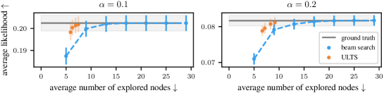
Figure 3: Comparison on trees, where the transition probabilities are sampled from a Dirichlet prior for two different values of the concentration parameter.

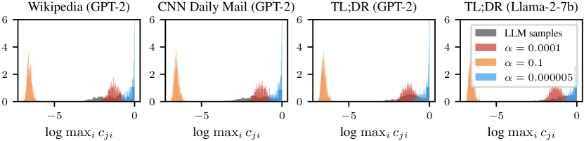
Figure 4: Distribution of the maximum of categorical distributions sampled from an LLM, as well as from Dirichlet priors with different concentration parameters.

5.2 Experiments with LLMs

We continue with off-model experiments, where we test ULTS for the decoding process of LLMs. We use GPT-2 [29] and Llama-2-7b [33] for text generation on articles from the Wikipedia [31], CNN Daily Mail [13], and Reddit TL;DR [36] datasets. Unless specified otherwise, we use the strategy in (2) for the selection and backup steps. See Appendix C for results with the other strategy and further dataset/setting. All experiments are done on single NVIDIA GeForce RTX 2080 Ti and NVIDIA A40 48GB GPUs for GPT-2 and Llama-2-7b, respectively.

Since many of the text samples in the Wikipedia dataset end with e.g., references instead of full sentences, we filter for text samples with at least $500$ tokens, resulting in a test set with $332$ token sequences (out of a random subset of originally $1000$ sequences). We use $200$ tokens as input and predict $20$ tokens. We do the same for the CNN Daily Mail dataset, where we end up with $790$ token sequences. We use context length of $300$ and generate $60$ tokens. We also include a summarization task, where the goal is to generate a $40$ token long summary of the input sequence. For this, we use $1000$ random samples from the TL;DR dataset. We use the full context of variable length. Note that we decode sequences of fixed length instead of stopping at the <EOS> token. This makes it easier to compare the different decoding methods with each other, as the overall likelihood of a sequence of course depends on its length. Additionally, see Appendix C for a machine translation experiment where ULTS stops at the <EOS> token.

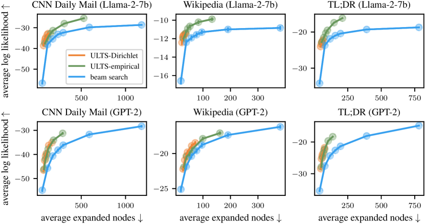
Figure 5: Decoding experiments with Llama-2-7b and GPT-2.

5.2.1 Choice of the prior

Before the decoding runs, we sampled a set $\mathcal{C}$ of Categorical distributions from the LLM on training sequences for each of the datasets and both of the LLLs. We used $1000$ samples for each of the datasets and LLMs we considered. They are used for the empirical prior, as well as training data for fitting the concentration parameter $\alpha$ of the Dirichlet prior. It is possible to adjust $\alpha$ using maximum likelihood optimization [26]. However, we have found that this did not work very well in our experiments: We suspect that it is either due to numerical problems of the optimization algorithm, or that the best fit for the Dirichlet distribution does not necessarily coincide with the best fit for the implied distribution of the (recursive) maximum. Figure 4 shows samples for the maximum of Categorical distributions returned by the LLM, as well as the distribution of the maximum of the Categorical distribution from a Dirichlet prior for $\alpha=10^{-1},10^{-4},5\times 10^{-6}$. While $\alpha=10^{-1}$ is in the order of the maximum likelihood estimator, the other values seem to fit better.

5.2.2 Comparison with baseline decoding methods

As the baseline we use the commonly-used beam search with beam width $k\in\{1,2,3,4,5,10,20\}$ [32]. These values capture the frequently-used beam widths [40]. Based on the results from the previous section, we run ULTS with both the Dirichlet prior with $\alpha=10^{-4}$ and the empirical prior. Moreover, we set $k_{\max}\in\{2,3,4,5,10,20\}$. We set $\epsilon$ to a default value of $0.1$. Figure 5 shows the results for GPT-2 and Llama-2-7b. The error bars indicate $\pm 1$ standard error of the mean based on all test sentences.

No matter the choice of $k_{\max}$ (and $k$), ULTS yields sequences with the same or a higher log-likelihood while expanding fewer nodes. For example in the summarization task with GPT-2, ULTS with the empirical prior and $k_{\text{max}}=20$ achieves an average log-likelihood of $-18.31$ while expanding only $137.90$ nodes. In contrast, beam search with $k=5$ returns sequences of average log-likelihood $-21.33$ even though expanding more nodes (196 nodes). This is the case for both choices of priors, with the empirical prior encouraging exploration a bit more. Figure 3 suggests that the distribution $\max_{i}c_{ji}$ is bimodal and not fully captured by the Dirichlet prior. In particular, our choice of Dirichlet prior is slightly too pessimistic. As a result, the search may stop too early and the available budget may not be fully utilized. However, the budget that is used, is used efficiently.

Our recommendation is thus as follows. When efficiency is the main goal, the Dirichlet prior is preferable—it performs similarly to beam search with smaller beam widths, while being more efficient. However, one must tune the value of $\alpha$. If the search performance is important and an additional tree exploration can be afforded (still more efficient than beam search), then the empirical prior is the best choice—it is also hyperparameter-free.

5.2.3 Runtime

Finally, we analyze the runtime overhead on top of the LLM’s forward pass due to ULTS. Figure 6 shows the wall-clock time per iteration, averaged over all sentences and all iterations, broken down into the time spent on the LLM’s forward pass and the time spent on sampling the optimal values and optimizing the acquisition function. The error bars indicate the $95\%$- confidence intervals. Results are shown for the experiments with $k_{\text{max}}=20$ and the Dirichlet prior—the empirical prior performs similarly since ULTS does not differentiate between them in Alg. 2. We note that the runtime overhead of ULTS is small compared to the time spent to do an LLM forward pass. However, note that our current implementation only expands one node of the search tree in each iteration and thereby only evaluate one token sequence per forward-pass. Depending on the available hardware, it may be advantageous to do batch node expansions.

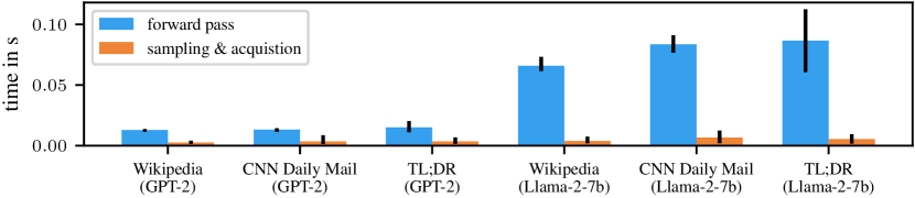
Figure 6: Average wall-clock time per iteration.

6 Conclusion

We have discussed our method, Uncertainty-guided Likelihood-Tree Search (ULTS), a probabilistic algorithm for the decoding process of large-language-model (LLM) search trees. Our method quantifies and leverages computational uncertainty over the maximum value of the optimization process. ULTS exploits the structure of the optimization problem—in particular, the concentration strength of the LLM softmax outputs—by putting a prior over the LLM’s softmax outputs, and use the implied posterior samples to guide exploration-exploitation in a non-myopic manner. It improves on the search efficiency of standard beam search by adapting the number of nodes expanded per level of the tree. In particular, ULTS expands fewer nodes than beam search, but achieves higher likelihood on average. As an interesting future direction, one can study the effect of using more sophisticated priors, e.g. where iid. is not assumed. One can also consider batched acquisition strategies, similar to batch Bayesian optimization techniques [7, 43]. Moreover, it is also interesting to take into account the uncertainty over the LLM’s outputs (e.g. in the context of Bayesian LLMs), and to incorporate (possibly uncertain) external rewards (such as ones coming from an RLHF-trained reward model) in addition to the current likelihood rewards.

Appendix A Further Discussions

A.1 Prior assumptions

The symmetry assumption for the Dirichlet prior on the LLM’s softmax outputs likely does not entirely hold—some words occur more often in natural language than others [16]. However, ULTS only requires access to the distribution over the maximum of the unexplored part of the search space and not over the arg max. The former is not affected by permutations of the entries in the categorical distributions, which is why we suspect that a symmetric Dirichlet distribution with sufficiently small concentration parameter is a good proxy. Moreover, the empirical prior can also be used to address this limitation, without incurring large overhead.

We assume the same prior for all sentences in a dataset. It could be, though, that some input prompts are easier to complete than others, and the corresponding LLM’s outputs are therefore generally have less entropy than on other those of other prompts. This could be counteracted by choosing a personalized hyper-parameter $\alpha$. This would require deriving the prior for multiple possible values of $\alpha$, which scales linearly with the number of possible values for $\alpha$. However, this can be precomputed (as in Alg. 1) such that it would not affect the costs during inference.

Appendix B Additional Experimental Details

URLs to the models and datasets used are provided below:

• Models:

  • https://huggingface.co/meta-llama/Llama-2-7b-hf

  • https://huggingface.co/openai-community/gpt2

• Datasets:

  • https://huggingface.co/datasets/wikipedia

  • https://huggingface.co/datasets/cnn_dailymail

  • https://huggingface.co/datasets/CarperAI/openai_summarize_tldr

For the additional machine translation experiment, we use the WMT-19 German to English dataset https://huggingface.co/facebook/wmt19-de-en and the following Llama-2-7b based translation model https://huggingface.co/kaitchup/Llama-2-7b-mt-German-to-English.

Appendix C Additional Experimental Results

C.1 On-model experiments

Figure 7 shows the additional results from the experiment on on-model samples from Dirichlet priors for $\alpha=0.5$ and $\alpha=0.8$ as described in Section 4.1 of the main text. Here, too, the probabilistic versions outperform beam search.

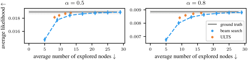
Figure 7: Comparison on trees, where the transition probabilities are sampled from a Dirichlet prior for two different values of the concentration parameter.

C.2 Machine translation

We compare ULTS and beam search in a machine translation task with 1000 randomly sampled sequences from the standard WMT-19 German to English dataset in Fig. 8. Unlike other settings we have used in the main text, here we terminate exploration once an <EOS> token is found. This setting is more ubiquitous in practice, but harder to compare in terms of likelihood due to the different sentence lengths. We observe that ULTS with the Dirichlet prior with $\alpha=0.0001$ underperform compared to beam search. This is because this prior induces less exploration. Indeed, when $\alpha$ is reduced, ULTS can utilize the search budget much more efficiently, achieving significantly better likelihoods while invoking much fewer LLM calls than beam search.

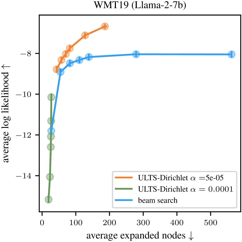
Figure 8: Machine translation results with the WMT-19 German-to-English dataset. All algorithms stop at the <EOS> token.

C.3 Alternative acquisition function

As discussed in Section 3.4, different selection (and hence backup) strategies can be utilized. Recall that all of our results so far are obtained using the “posterior descendant” strategy defined in (2). Here, we show the corresponding results where the other strategy (“posterior”) is used instead.

First, Fig. 9 shows results under the same setting as in the main text, but both ULTS-Dirichlet and ULTS-Emp use the “posterior” strategy instead. We noticed that this strategy also performs well—it is more efficient than beam search. Moreover, it also achieves better or similar likelihood than beam search in Llama-2-7b.

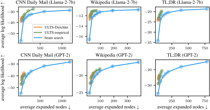
Figure 9: Decoding experiments with Llama-2-7b and GPT-2 with the “posterior” strategy.

We further compare the “posterior” strategy compared to the “posterior descendant” strategy in Fig. 10. We notice that the “posterior” strategy tends to underexplore compared to the “posterior descendant” strategy. Hence, we use and recommend the “posterior descendant” strategy by default.

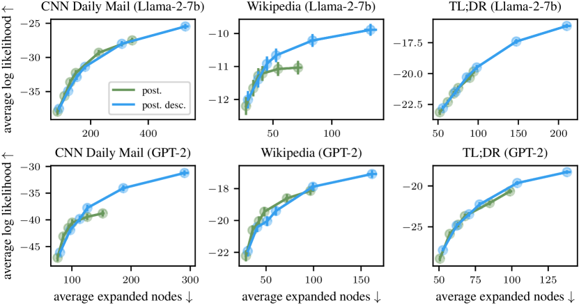
Figure 10: “Posterior” vs. “posterior descendant” acquisition function.

References

- AbouRizk et al. [1994] Simaan M AbouRizk, Daniel W Halpin, and James R Wilson. Fitting Beta distributions based on sample data. Journal of Construction Engineering and Management, 120(2), 1994.
- Balandat et al. [2020] Maximilian Balandat, Brian Karrer, Daniel Jiang, Samuel Daulton, Ben Letham, Andrew G Wilson, and Eytan Bakshy. BoTorch: A framework for efficient Monte-Carlo Bayesian optimization. In NeurIPS, 2020.
- Chowdhery et al. [2023] Aakanksha Chowdhery, Sharan Narang, Jacob Devlin, Maarten Bosma, Gaurav Mishra, Adam Roberts, Paul Barham, Hyung Won Chung, Charles Sutton, Sebastian Gehrmann, et al. PaLM: Scaling language modeling with pathways. JMLR, 24(240), 2023.
- Feng et al. [2023] Xidong Feng, Ziyu Wan, Muning Wen, Ying Wen, Weinan Zhang, and Jun Wang. Alphazero-like tree-search can guide large language model decoding and training. arXiv preprint arXiv:2309.17179, 2023.
- Freitag and Al-Onaizan [2017] Markus Freitag and Yaser Al-Onaizan. Beam search strategies for neural machine translation. In ACL Workshop on Neural Machine Translation, 2017.
- Garnett [2023] Roman Garnett. Bayesian Optimization. Cambridge University Press, 2023.
- González et al. [2016] Javier González, Zhenwen Dai, Philipp Hennig, and Neil Lawrence. Batch Bayesian optimization via local penalization. In AISTATS, 2016.
- Grosse et al. [2021] Julia Grosse, Cheng Zhang, and Philipp Hennig. Probabilistic DAG search. In UAI, 2021.
- Hao et al. [2023] Shibo Hao, Yi Gu, Haodi Ma, Joshua Jiahua Hong, Zhen Wang, Daisy Zhe Wang, and Zhiting Hu. Reasoning with language model is planning with world model. arXiv preprint arXiv:2305.14992, 2023.
- Hart et al. [1968] Peter E Hart, Nils J Nilsson, and Bertram Raphael. A formal basis for the heuristic determination of minimum cost paths. IEEE transactions on Systems Science and Cybernetics, 4(2), 1968.
- Hennig et al. [2010] Philipp Hennig, David Stern, and Thore Graepel. Coherent inference on optimal play in game trees. In AISTATS, 2010.
- Hennig et al. [2022] Philipp Hennig, Michael A Osborne, and Hans P Kersting. Probabilistic Numerics: Computation as Machine Learning. Cambridge University Press, 2022.
- Hermann et al. [2015] Karl Moritz Hermann, Tomas Kocisky, Edward Grefenstette, Lasse Espeholt, Will Kay, Mustafa Suleyman, and Phil Blunsom. Teaching machines to read and comprehend. In NIPS, 2015.
- Hernández-Lobato et al. [2017] José Miguel Hernández-Lobato, James Requeima, Edward O Pyzer-Knapp, and Alán Aspuru-Guzik. Parallel and distributed Thompson sampling for large-scale accelerated exploration of chemical space. In ICML, 2017.
- Holtzman et al. [2019] Ari Holtzman, Jan Buys, Li Du, Maxwell Forbes, and Yejin Choi. The curious case of neural text degeneration. In ICLR, 2019.
- Kingsley Zipf [1932] George Kingsley Zipf. Selected Studies of the Principle of Relative Frequency in Language. Harvard University Press, 1932.
- Kochenderfer [2015] Mykel J Kochenderfer. Decision making under uncertainty: theory and application. MIT Press, 2015.
- Koehn et al. [2003] Philipp Koehn, Franz Josef Och, and Daniel Marcu. Statistical phrase-based translation. In HLT-NAACL, 2003.
- Kristiadi et al. [2023] Agustinus Kristiadi, Alexander Immer, Runa Eschenhagen, and Vincent Fortuin. Promises and pitfalls of the linearized Laplace in Bayesian optimization. In AABI, 2023.
- Kristiadi et al. [2024] Agustinus Kristiadi, Felix Strieth-Kalthoff, Marta Skreta, Pascal Poupart, Alán Aspuru-Guzik, and Geoff Pleiss. A sober look at LLMs for material discovery: Are they actually good for Bayesian optimization over molecules? In ICML, 2024.
- Kushner [1964] Harold J Kushner. A new method of locating the maximum point of an arbitrary multipeak curve in the presence of noise. J. Basic Eng, 1964.
- Leblond et al. [2021] Rémi Leblond, Jean-Baptiste Alayrac, Laurent Sifre, Miruna Pislar, Jean-Baptiste Lespiau, Ioannis Antonoglou, Karen Simonyan, and Oriol Vinyals. Machine translation decoding beyond beam search. arXiv preprint arXiv:2104.05336, 2021.
- Liu et al. [2023] Jiacheng Liu, Andrew Cohen, Ramakanth Pasunuru, Yejin Choi, Hannaneh Hajishirzi, and Asli Celikyilmaz. Don’t throw away your value model! making PPO even better via value-guided Monte-Carlo Tree Search decoding. arXiv e-prints, 2023.
- Meister et al. [2020] Clara Meister, Tim Vieira, and Ryan Cotterell. Best-first beam search. TACL, 8, 2020.
- Meister et al. [2021] Clara Meister, Martina Forster, and Ryan Cotterell. Determinantal beam search. arXiv preprint arXiv:2106.07400, 2021.
- Minka [2000] Thomas Minka. Estimating a Dirichlet distribution, 2000.
- Minka [2001] Thomas Peter Minka. A family of algorithms for approximate Bayesian inference. PhD thesis, Massachusetts Institute of Technology, 2001.
- Močkus [1975] Jonas Močkus. On Bayesian methods for seeking the extremum. In Optimization Techniques IFIP Technical Conference, 1975.
- Radford et al. [2019] Alec Radford, Jeffrey Wu, Rewon Child, David Luan, Dario Amodei, Ilya Sutskever, et al. Language models are unsupervised multitask learners. OpenAI Blog, 2019.
- Rasmussen and Williams [2005] Carl Edward Rasmussen and Christopher K. I. Williams. Gaussian Processes in Machine Learning. The MIT Press, 2005.
- See et al. [2017] Abigail See, Peter J. Liu, and Christopher D. Manning. Get to the point: Summarization with pointer-generator networks. In ACL, 2017.
- Stiennon et al. [2020] Nisan Stiennon, Long Ouyang, Jeffrey Wu, Daniel Ziegler, Ryan Lowe, Chelsea Voss, Alec Radford, Dario Amodei, and Paul F Christiano. Learning to summarize with human feedback. In NeurIPS, 2020.
- Touvron et al. [2023] Hugo Touvron, Louis Martin, Kevin Stone, Peter Albert, Amjad Almahairi, Yasmine Babaei, Nikolay Bashlykov, Soumya Batra, Prajjwal Bhargava, Shruti Bhosale, et al. Llama 2: Open foundation and fine-tuned chat models. arXiv preprint arXiv:2307.09288, 2023.
- Vaswani et al. [2017] Ashish Vaswani, Noam Shazeer, Niki Parmar, Jakob Uszkoreit, Llion Jones, Aidan N Gomez, Łukasz Kaiser, and Illia Polosukhin. Attention is all you need. In NIPS, 2017.
- Vijayakumar et al. [2018] Ashwin K Vijayakumar, Michael Cogswell, Ramprasath R Selvaraju, Qing Sun, Stefan Lee, David Crandall, and Dhruv Batra. Diverse beam search: Decoding diverse solutions from neural sequence models. In AAAI, 2018.
- Völske et al. [2017] Michael Völske, Martin Potthast, Shahbaz Syed, and Benno Stein. TL;DR: Mining Reddit to learn automatic summarization. In Workshop on New Frontiers in Summarization, 2017.
- Wang et al. [2022] Peng Wang, An Yang, Rui Men, Junyang Lin, Shuai Bai, Zhikang Li, Jianxin Ma, Chang Zhou, Jingren Zhou, and Hongxia Yang. Ofa: Unifying architectures, tasks, and modalities through a simple sequence-to-sequence learning framework. In ICML, 2022.
- Wang and Jegelka [2017] Zi Wang and Stefanie Jegelka. Max-value entropy search for efficient Bayesian optimization. In ICML, 2017.
- Wang et al. [2016] Zi Wang, Bolei Zhou, and Stefanie Jegelka. Optimization as estimation with Gaussian processes in bandit settings. In AISTATS, 2016.
- Wiher et al. [2022] Gian Wiher, Clara Meister, and Ryan Cotterell. On decoding strategies for neural text generators. TACL, 10, 2022.
- Wilson and Izmailov [2020] Andrew G Wilson and Pavel Izmailov. Bayesian deep learning and a probabilistic perspective of generalization. In NeurIPS, 2020.
- Wolf et al. [2020] Thomas Wolf, Lysandre Debut, Victor Sanh, Julien Chaumond, Clement Delangue, Anthony Moi, Pierric Cistac, Tim Rault, Remi Louf, Morgan Funtowicz, Joe Davison, Sam Shleifer, Patrick von Platen, Clara Ma, Yacine Jernite, Julien Plu, Canwen Xu, Teven Le Scao, Sylvain Gugger, Mariama Drame, Quentin Lhoest, and Alexander Rush. Transformers: State-of-the-art natural language processing. In EMNLP, 2020.
- Wu and Frazier [2016] Jian Wu and Peter Frazier. The parallel knowledge gradient method for batch Bayesian optimization. In NIPS, 2016.
- Zhang et al. [2020] Jingqing Zhang, Yao Zhao, Mohammad Saleh, and Peter Liu. Pegasus: Pre-training with extracted gap-sentences for abstractive summarization. In ICML, 2020.
- Zhang et al. [2023] Shun Zhang, Zhenfang Chen, Yikang Shen, Mingyu Ding, Joshua B Tenenbaum, and Chuang Gan. Planning with large language models for code generation. In ICLR, 2023.
- Zhu et al. [2019] Jinhua Zhu, Yingce Xia, Lijun Wu, Di He, Tao Qin, Wengang Zhou, Houqiang Li, and Tieyan Liu. Incorporating BERT into neural machine translation. In ICLR, 2019.