The negative BAO shift in the Ly$\alpha$ forest from cosmological simulations

Abstract

We present the first measurement of the Ly$\alpha$ forest BAO shift parameter from cosmological simulations. In particular, we generate a suite of $1000$ accurate effective field-level bias-based Ly$\alpha$ forest simulations of volume $V=(1\,h^{-1}\,{\rm Gpc})^{3}$ at $z=2$, both in real and redshift space, calibrated upon two fixed-and-paired cosmological hydrodynamic simulations. To measure the BAO, we stack the three-dimensional power spectra of the $1000$ different realizations, compute the average, and use a model accounting for a proper smooth-peak component decomposition of the power spectrum, to fit it via an efficient Markov Chain Monte Carlo scheme estimating the covariance matrices directly from the simulations. We report the BAO shift parameters to be $\alpha=0.9969^{+0.0014}_{-0.0014}$ and $\alpha=0.9905^{+0.0027}_{-0.0027}$ in real and redshift space, respectively. We also measure the bias $b_{\rm lya}$ and the BAO broadening parameter $\Sigma_{\rm nl}$, finding $b_{\rm lya}=-0.1786^{+0.0001}_{-0.0001}$ and $\Sigma_{\rm nl}=3.87^{+0.20}_{-0.20}$ in real space, and $b_{\rm lya}=-0.073^{+0.005}_{-0.004}$ and $\Sigma_{\rm nl}=6.55^{+0.23}_{-0.22}$ in redshift space. Moreover, we measure the linear Kaiser factor $\beta_{\rm lya}=1.39^{+0.24}_{-0.18}$ from the isotropic redshift space fit. Overall, we find evidence for a negative shift of the BAO peak at the $\sim 2.2\sigma$ and $\sim 3.5\sigma$ level in real and redshift space, respectively. This work sets new important theoretical constraints on the Ly$\alpha$ forest BAO scale and offers a potential solution to the tension emerging from previous observational analysis, in light of ongoing and upcoming Ly$\alpha$ forest spectroscopic surveys, such as DESI, PFS, and WEAVE-QSO.

1 Introduction

The Baryon Acoustic Oscillations (BAO) are standard rulers to measure cosmic distances (Sunyaev & Zeldovich, 1970; Peebles & Yu, 1970; Seo & Eisenstein, 2003; Blake & Glazebrook, 2003). They consist in the excess clustering observed at comoving $r\sim 150\,h^{-1}\,{\rm Mpc}$ in the two-point correlation function and at different wavenumbers in the power spectrum of biased tracers of the dark matter field, and arise as a result of the propagation of acoustic density waves and the coupling between photons and plasma in the early Universe.

The first detection of the BAO independently by the Baryon Oscillation Spectroscopic Survey (BOSS) and the 2dF Galaxy Redshift Survey (2dFGRS) collaborations using galaxy clustering (Eisenstein et al., 2005; Cole et al., 2005) confirmed this prediction from the standard theory of cosmology. Since then, BAO studies have reported several other detections of the acoustic peak using different tracers of large-scale structure, supporting the paradigm described above (Beutler et al., 2011; Anderson et al., 2012; Busca et al., 2013; Slosar et al., 2013; Font-Ribera et al., 2014; Delubac et al., 2015; Kitaura et al., 2016; Beutler et al., 2017; Bautista et al., 2017; du Mas des Bourboux et al., 2020; Zhao et al., 2022). The DESI (Levi et al., 2013) and Euclid (Amendola et al., 2018) surveys promise to achieve percent accuracy in the determination of the position of the BAO peak. Recently, DESI reported the detection of BAO over an effective volume of $V\sim 18\,{\rm Gpc}^{3}$ and in six different redshift bins by relying on distinct tracers, with highest precision and significance of $\sim 0.83\%$ and $\sim 9.1\sigma$, respectively, at $z\sim 0.93$ (DESI Collaboration et al., 2024a).

The BAO peak position of the dark matter field in linear theory can be accurately predicted as a function of cosmology by means of a Boltzmann equation solver (e.g. Lewis & Challinor, 2011; Blas et al., 2011). However, the gravitational growth of structures induces the well-known distortions of the BAO. In particular, the nonlinear evolution of the density field broadens the BAO — thus making the BAO measurements less precise — and typically induces a systematic subpercent shift in the acoustic peak position whose magnitude and sign depend on the investigated cosmological tracer. To tackle the first problem — which goes beyond the scope of this work — a plethora of reconstruction techniques based on de-evolving cosmic structures in time have been put forward, and shown to successfully reduce the uncertainty on the BAO peak position without biasing the peak position itself (e.g. Eisenstein et al., 2007a; Schmittfull et al., 2015). As for the latter aspect, the evolved dark matter field itself, together with galaxies and haloes tracing high-density environments, have been reported to display a positive subpercent (typically of order $\lesssim 0.5\%$) BAO shift with respect to the prediction from linear theory, whereas the position of the BAO imprinted in low-density environments presents a negative shift of the same magnitude (Sherwin & Zaldarriaga, 2012; Achitouv & Blake, 2015; Kitaura et al., 2016; Neyrinck et al., 2018; Hernández-Aguayo et al., 2020). Finally, redshift space distortions (RSD) are also known to introduce a further positive contribution to the total shift in the BAO peak, also of order $\lesssim 0.5\%$ (e.g. Prada et al., 2016).

In this context, the Ly$\alpha$ forest — the ensemble of absorption lines imprinted on quasar spectra when light rays encounter intervening HI clouds — has witnessed a recent growth in interest. In fact, the Ly$\alpha$ forest offers high-$z$ measurements of the BAO scale, and so a rare and robust probe of dark energy at high cosmic noon. Since the first measurements (Font-Ribera et al., 2014; Bautista et al., 2017; du Mas des Bourboux et al., 2020) – which reported a $4-5\%$ positive shift in the BAO peak along the parallel direction to the line of sight from the BOSS and eBOSS surveys — the Ly$\alpha$ forest BAO scale has been in tension with the $\Lambda$CDM model. The most recent measurements of the Ly$\alpha$ forest BAO scale from the DESI survey (DESI Collaboration et al., 2024b) sharpened the tension with eBOSS Ly$\alpha$ forest BAO results even more.

On the other hand, theoretical studies of the Ly$\alpha$ forest BAO relying on simple bias models — such as purely analytical studies (Seljak, 2012; Chen et al., 2021) and approximate simulations (White et al., 2010; Hadzhiyska et al., 2023) — have not reported measurements of any potential shift of the BAO peak position.

In this work, we present the first determination of the Ly$\alpha$ forest BAO peak position and its shift with respect to the prediction from the linear theory of structure formation in $\Lambda$CDM models, based on accurate fast simulations, calibrated on full cosmological hydrodynamic simulations with baryonic physics of star formation and supernova feedback.

The paper is structured as follows. In §2 we present the two fixed-and-paired reference simulations that we use for calibration. In §3 we summarize the model that we adopt to generate the simulations used here. §4 outlines the procedure employed to fit the BAO from the set of simulations. §5 presents the results and develops a theoretical intuition of them. We conclude in §6.

2 Fixed-and-paired cosmological hydrodynamic simulations

In this work, we measure the Ly$\alpha$ forest BAO peak position from a set of fast Ly$\alpha$ forest simulations, generated using a bias model calibrated on two fixed-and-paired (Angulo & Pontzen, 2016) cosmological hydrodynamical simulations. Such reference hydrodynamic simulations were run with the cosmological smoothed-particle hydrodynamics (SPH) code GADGET3-OSAKA (Aoyama et al., 2018; Shimizu et al., 2019; Nagamine et al., 2021), a modified version of GADGET-3 and a descendant of the popular $N$-body/SPH code GADGET-2 (Springel, 2005). It embeds a comoving volume, $V=(500h^{-1}\text{Mpc})^{3}$, and $N=2\times 1024^{3}$ particles of mass $m_{\rm DM}=8.43\times 10^{9}h^{-1}\text{M}_{\odot}$ for DM particles and $m_{\rm gas}=1.57\times 10^{9}h^{-1}\text{M}_{\odot}$ for gas particles.

The gravitational softening length was set to $\epsilon_{g}=16h^{-1}$ kpc (comoving), but we allowed the baryonic smoothing length to become as small as $0.1\epsilon_{g}$. This means that the minimum baryonic smoothing at $z=2$ is about physical $533\,h^{-1}$ pc. The star formation and supernova feedback were treated as described in Shimizu et al. (2019). The code also contains important refinements, such as the density-independent formulation of SPH and the time-step limiter (Saitoh & Makino, 2009, 2013; Hopkins et al., 2013).

The main baryonic processes that shape the evolution of the gas are photo-heating, photo-ionization under the UV background radiation (Haardt & Madau, 2012), and radiative cooling. All of these processes are taken into account and solved by the Grackle library (Smith et al., 2017), which determines the chemistry for atomic (H, D and He) and molecular (H₂ and HD) species. The chemical enrichment from supernovae is also treated with the CELib chemical evolution library (Saitoh, 2017). The initial conditions are generated at redshift $z=99$ using MUSIC2 (Hahn et al., 2021), with cosmological parameters taken from the 2020 data release of the Planck collaboration (Planck Collaboration et al., 2020).

We use the output of the simulation at $z=2$ reading gas properties and compute the Ly$\alpha$ forest flux field by first obtaining the HI optical depth $\tau$ by means of a line-of-sight integration as follows (Nagamine et al., 2021):

$$\tau(x_{0})=\frac{\pi e^{2}}{m_{e}c}\int f\,\phi(x-x_{0})\,n_{\rm HI}(x)\,dx\,$$ (1)

where $e$, $m_{e}$, $c$, $n_{\rm HI}$, $f$, $x$ and $\phi$ denote, respectively, the electron charge, electron mass, speed of light in vacuum, HI number density, absorption oscillator strength, line-of-sight coordinate, and the parametrization of the Voigt spectral line profile. Where necessary, relevant quantities (e.g., HI number density) were previously interpolated on the mesh according to the SPH kernel of the simulation.

We interpolated the Ly$\alpha$ forest fields in real and in redshift space onto a $1024^{3}$-cell cubic mesh — i.e. at the native resolution of the simulation — using a cloud-in-cell mass assignment scheme (Hockney & Eastwood, 1981).

3 Fast Lyman-$\alpha$ forest simulations

We adopt the novel nonlocal Fluctuating Gunn-Peterson approximation (NL FGPA) model (Sinigaglia et al., 2024), which builds on the standard FGPA. Briefly, the FGPA models the Ly$\alpha$ forest opacity $\tau$ as a power law of the underlying dark matter field overdensity $\delta$ as $\tau=A(1+\delta)^{\gamma}$ (Bi, 1993; Hui et al., 1997; Croft et al., 1998). Starting from this point, the NL FGPA drops the assumption that a unique scaling relation holds over the full probed cosmological volume, and introduces instead a dependence on the cosmic web environment through the T-web classification (Hahn et al., 2007). After obtaining the gravitational potential $\phi(\vec{r})$ in Eulerian coordinates $\vec{r}$ by solving the Poisson equation $\phi(\vec{r})=\nabla^{2}\delta(\vec{r})$, the rank-2 gravitational tidal field tensor is defined as $\mathcal{T}_{ij}(\vec{r})=\partial_{i}\partial_{j}\phi(\vec{r})$, with eigenvalues $\lambda_{1}\geq\lambda_{2}\geq\lambda_{3}$. At this point, given the mesh discretization of the dark matter density field, a cell is classified as belonging to a knot if $\lambda_{1},\lambda_{2},\lambda_{3}\geq 0$, to a filament if $\lambda_{1},\lambda_{2}\geq 0,\lambda_{3}<0$, to a sheet if $\lambda_{1}\geq 0,\lambda_{2},\lambda_{3}<0$, or to a void if $\lambda_{1},\lambda_{2},\lambda_{3}<0$. The resulting nonlocal bias model for the Ly$\alpha$ forest becomes hence sensitive to the anisotropic clustering of the surrounding environment and encodes information up the third order of an Eulerian perturbative renormalized bias expansion (McDonald & Roy, 2009; Kitaura et al., 2022), i.e. all the orders which contribute to the clustering of the summary statistics studied herein (Werner & Porciani, 2020).

In addition to the parametrization of the geometry of the cosmic web, the NL FGPA includes two multiplicative threshold bias factors $\exp(\pm\delta/\delta^{*})$ controlled by a scale parameter $\delta^{*}$ — acting as a boosting (‘$+$’ sign) and cutoff terms (‘$-$’ sign) — and a stochastic additive term $\epsilon$ sampled from a negative binomial distribution modeling a stochastic bias component. The final model reads:

$$\tau=A_{i}(1+\delta)^{\gamma_{i}}\,\exp(\delta/\delta^{*}_{i})+\epsilon_{i}\quad,$$ (2)

with $i=${knots, filaments, sheets, voids}.

To include the effect of peculiar velocities and obtain the Ly$\alpha$ forest in redshift space (as is observed), we perform a cell-level mapping from real to redshift space (Sinigaglia et al., 2021, 2022, 2024), including a velocity bias contribution in the customary redshift space distortions formula (Kaiser, 1984):

$$\vec{s}=\vec{r}\,+\,b_{v}\frac{(\vec{v}\cdot\hat{r})\,\hat{r}}{aH}$$ (3)

where $\vec{r}$ and $\vec{s}$ indicate real-space and redshift-space Eulerian coordinates, $b_{v}$ is the velocity bias, and $a$ and $H$ are the scale factor and the Hubble parameter at the studied redshift. The velocity field $\vec{v}=\vec{v}_{\rm coh}\,+\,\vec{v}_{\rm qvm}$ is modeled as the sum of a large-scale coherent flow component $\vec{v}_{\rm coh}$ — which consists in the velocity field itself interpolated on the mesh — and a small-scale quasi-virialized motion component $\vec{v}_{\rm qvm}$, a component randomly-sampled from a Gaussian distribution with zero mean and density-dependent standard deviation: $\vec{v}_{\rm qvm}\curvearrowright\mathcal{G}(0,\sigma)$, $\sigma=B(1+\delta)^{\beta}$, with $B$ and $\beta$ free parameters. The latter component is included because the mesh interpolation of the particle velocities smooths out the contribution below the scale of the cell, thereby damping the velocity dispersion component. Within the NL FGPA approximation, we always consider the dark matter velocity field instead of the one of the gas, even though we are modeling a baryon observable. This is done because the model needs to be generalized to any structure formation model, and approximated gravity solvers do not model any gas properties and yield just (approximated) dark matter velocities. The potential velocity bias between gas and dark matter arising from this assumption is then modeled and reabsorbed in the $b_{v}$ factor.

Eventually, the Ly$\alpha$ forest transmitted flux (i.e., normalized to the quasar continuum) is obtained as $F=\exp(-\tau)$.

We refer the reader to the paper presenting the NL FGPA model (Sinigaglia et al., 2024), for a thorough discussion of the improvements with respect to previous implementations of the FGPA.

Within this framework, we first calibrate the NL FGPA model on the reference simulations and reproduce their summary statistics. We obtain the dark matter field by applying the ALPT structure formation model (Kitaura & Hess, 2013) with phase-space mapping (Abel et al., 2012) on a grid of $N_{p}=256^{3}$ cells and a comoving volume $V=(500\,h^{-1}\,{\rm Mpc})^{3}$ (physical cell resolution $l\sim 1.95\,h^{-1}\,\rm{Mpc}$). In particular, we consider the same initial conditions as the reference simulations downsampled to the target resolution, and evolve them using ALPT down to $z=2$. After this first phase, to correct for the inaccuracy of the gravity solver and for the lack of resolution, we apply a rank-ordering nonlinear transform and force the approximated dark matter density field to follow the same distribution as the nonlinear evolved dark matter field from the N-body simulation. Afterward, we apply the NL FGPA model to predict the Ly$\alpha$ forest, both in real and in redshift space. We apply a rank-ordering transform also of the velocity field obtained with ALPT to the one from the cosmological simulation, in order to have a set of reliable nonlinear peculiar velocities to map the density field from real to redshift space. The parameters of the model are estimated by jointly fitting the flux probability distribution function (PDF) and the 3D power spectrum (for $k\leq 0.5\,h\,{\rm Mpc}^{-1}$) using a global optimizer implementing a genetic algorithm. In particular, to prevent the risk of overfitting of just one cosmic realization, we jointly fit the summary statistics of the two fixed-and-paired simulations.

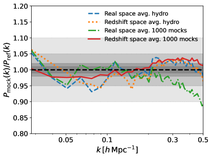
Figure 1: Ratios $P_{\rm mock}/P_{\rm ref}$ of three-dimensional Ly$\alpha$ forest power spectra. The blue dashed and orange dotted lines show the ratios of the average of the power spectra of the pair of simulations in real and redshift space, respectively. The green dashed-dotted and red solid lines display instead the power spectrum ratios of the mean of $1000$ mocks in real space and in redshift space, respectively. The gray dashed regions stand for $1\%$, $2\%$, $5\%$, and $10\%$ deviations, from the darkest to the lightest.

Figure 1 shows the resulting calibration of the 3D power spectrum. The blue dashed and orange dotted lines show the ratios $P_{\rm mock}(k)/P_{\rm ref}(k)$ of the average of the power spectra simulation pairs, in real and redshift space, respectively. The average and maximum deviations in the power spectrum up to $k\sim 0.5\,h\,{\rm Mpc}^{-1}$ are $\sim 2.2\%$ and $\sim 5.3\%$ in real space, and $\sim 2.3\%$ and $\sim 6.2\%$ in redshift space. These figures are reduced to $\sim 1.8\%$ and $\sim 3.8\%$ in real space, and $\sim 2\%$ and $\sim 3.4\%$ in redshift space if we restrict the analysis to $0.1<k<0.5\,h\,{\rm Mpc}^{-1}$, i.e. around the BAO scale. We also show power spectrum ratios for the mean of $1000$ mocks in real space (green dashed-dotted) and in redshift space (red solid), which achieves comparable accuracy to the one the calibrated power spectra in the $k$ range of interest. This demonstrates that the generalization of the calibration to random initial conditions yields substantially unbiased power spectra.

Using the calibrated parameters, we then generate $1000$ Ly$\alpha$ forest realizations of comoving volume $V=(1\,h^{-1}\,{\rm Gpc})^{3}$ (a factor $8$ larger than the one used for the calibration), both in real and in redshift space. In this case, the initial conditions are generated randomly, self-consistently convolving the white noise with the same input linear power spectrum as the simulations used for calibration.

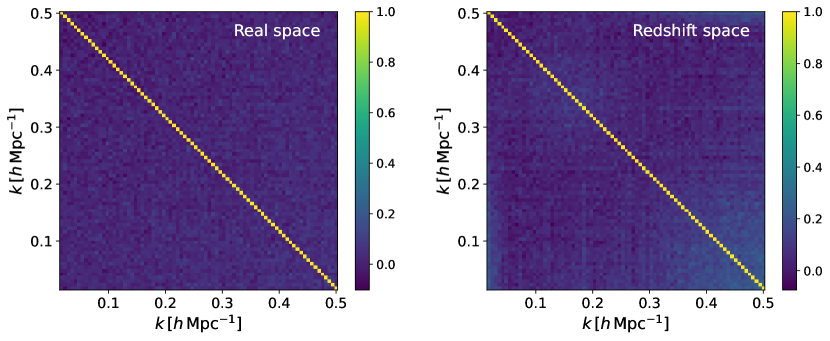
Figure 2: Correlation coefficient matrices in real (left) and redshift space (right), as obtained from the $1000$ fast Ly$\alpha$ forest simulations generated in this work.

4 Fitting the BAO of the Lyman-$\alpha$ forest

We fit the Ly$\alpha$ forest three-dimensional power spectrum and derive the position of the acoustic peak and its shift parameter with respect to linear theory as follows.

We decompose the power spectrum into the sum of a smooth (no-wiggles) and peak (oscillating) components. In particular, we express the model for the power spectrum $P_{\rm model}(k)$ as (e.g. du Mas des Bourboux et al., 2020):

$$P_{\rm model}(\vec{k})=b_{\rm lya}^{2}\,(1+\beta_{\rm lya}\,\mu_{k}^{2})^{2}\,P_{\rm ql}(\vec{k})\,F_{\rm nl}(\vec{k})$$ (4)

where $\vec{k}=(k_{\parallel},k_{\perp})$ is the Fourier-space mode vector of modulus $k=|\vec{k}|$ and $\mu_{k}=k_{\parallel}/k$, $b_{\rm lya}$ is the bias parameter, $\beta_{\rm lya}$ is the linear redshift space distortions parameter, $P_{\rm ql}$ is the quasi-linear matter power spectrum (described in detail below), $F_{\rm nl}$ is a transfer function accounting for the nonlinear growth of structures and modelling the nonlinear scales in the power spectrum. Differently from the main observational analyses carried out thus far in the literature, we do not include the correction term $G(\vec{k})$ accounting for the damping induced by the binning of the correlation function in $(r_{\parallel},r_{\perp})$ as we limit here our analysis to Fourier space and do not Fourier-transform the power spectrum into the correlation function in configuration space.

The quasi-linear power spectrum is modelled, as anticipated, as the sum of a smooth and a peak component:

$$P_{\rm ql}=P_{\rm s}(k)+A(k)P_{\rm p}(k/\alpha)\exp\left(-\frac{k^{2}\Sigma_{\rm nl}^{2}}{2}\right)$$ (5)

where $P_{\rm s}$ is the smooth component of the power spectrum obtained via empirical cubic spline interpolation, $P_{\rm p}=P_{\rm lin}-P_{\rm s}$ is the peak component with $P_{\rm lin}$ the linear power spectrum, $A(k)$ is a function describing the amplitude of the BAO, $\Sigma_{\rm nl}$ is a free parameter modeling the nonlinear broadening of the BAO peak, and $\alpha$ is the ‘shift’ parameter, inducing a stretch ($\alpha<1$) or a compression ($\alpha>1$) of the power spectrum along the $k$ axis. Following du Mas des Bourboux et al. (2020), we reduce the function $A(k)$ to a $k$-independent parameter $A$, and find that this choice is sufficient to provide a good fit. Defining $\Delta^{2}(k)=k^{3}P_{l}(k)/(2\pi^{3})$ , the transfer function $F_{\rm nl}$ is based on the following model (Arinyo-i-Prats et al., 2015):

$$F_{\rm nl}=\exp\left\{q_{1}\Delta^{2}(k)\,\left[1-\left(\frac{k}{k_{v}}\right)^{a_{v}}\mu^{b_{v}}\right]-\left(\frac{k}{k_{p}}\right)^{2}\right\}$$ (6)

with $q_{1}$, $a_{v}$, $k_{v}$, $b_{v}$, and $k_{p}$ free parameters. Most of these parameters affect the shape of the Ly$\alpha$ forest power scale at highly nonlinear scales.

We perform the fit as follows. First, we compute the covariance matrices in real and redshift space from the $1000$ simulations, which are shown in Fig. 2. The covariance matrix in real space (left) does not show any evident off-diagonal correlation, while the one in redshift space (right) features weak off-diagonal correlations at $k\gtrsim 0.4\,h\,{\rm Mpc}^{-1}$. Afterwards, we stack the $1000$ Ly$\alpha$ forest realizations and fit the average power spectrum. We first determine the maximum likelihood best-fit solution, using the covariance matrices computed above. Then, we use the solution of the maximum likelihood estimation as an initial guess for a full Markov-Chain Monte Carlo sampling of the posterior distributions, assuming a Gaussian likelihood and flat priors around the maximum likelihood solution. The fit is performed over at $0.05<k<0.25\,h\,{\rm Mpc}^{-1}$, as it is the $k$-interval which encompasses the three BAO peaks, as will be shown in Fig. 3. The further BAO peaks are found to be too degraded by nonlinear evolution to be reliably included in the fit.

5 Results and discussion

We show the resulting fit of the BAO of the average Ly$\alpha$ forest power spectrum from our $1000$ realizations in Fig. 3, in real (top) and redshift space (bottom). The fit yields a $\chi^{2}/{\rm dof=1.13}$ in real space and $\chi^{2}/{\rm dof=1.05}$ in redshift, i.e. the fits are regarded to be high quality. As can be noticed, in redshift space the third BAO peak is already damped by the nonlinear growth of structure and RSD. Nonetheless, we have explicitly verified that including it or not in the fitting procedure has a negligible impact on the results.

Fig. 4 and Fig. 5 show the posterior distributions of the model parameters in real and redshift space, respectively. We quote as the best-fit value of each model parameter the $50$th percentile of its posterior, and as associated uncertainties the combination of percentiles $84$th–$50$th (upper) and $50$th–$16$th (lower).

We find the following BAO shift parameters: $\alpha=0.9969^{+0.0014}_{-0.0014}$ in real space, $\alpha=0.9905^{+0.0027}_{-0.0027}$ in in redshift space. Overall, we find evidence for a negative shift of the BAO peak, both in real and in redshift space, at $\sim 2.2\sigma$ and $\sim 3.5\sigma$, respectively. This result is qualitatively in agreement with measurements from other cosmological tracers residing in underdense regions, such as galaxies in cosmic voids, which have been shown to display a negative shift in the BAO peak. Moreover, we measure a difference at $\sim 2.2\sigma$ significance between the real and redshift space BAO shift, hinting towards an enhancement of the shift due to redshift space distortions, as previously known from the literature (e.g. Eisenstein et al., 2007b; Prada et al., 2016). These findings are compatible within statistical uncertainties with the most recent measurements of the Ly$\alpha$ forest BAO from the DESI collaboration (DESI Collaboration et al., 2024b). Remarkably, also DESI reported a negative median value of the Ly$\alpha$ forest BAO shift parameter, even though such a shift is not statistically significant given the measured uncertainties.

We also measure explicitly for the first time the nonlinear broadening parameter $\Sigma_{\rm nl}$, finding $\Sigma_{\rm nl}=3.87^{+0.20}_{-0.20}$ in real space, and $\Sigma_{\rm nl}=6.56^{+0.23}_{-0.22}$ in redshift space — in excellent agreement with the prediction at similar redshift from linear theory corrected for nonlinear evolution reported by Hadzhiyska et al. (2023) — corresponding to $\sim 19.3\sigma$ and $\sim 30\sigma$ deviations from pure linear theory uncorrected for nonlinear evolution, respectively. Moreover, we find a difference between the real and the redshift space best-fit at $\sim 8.8\sigma$, with $\Sigma_{\rm nl}$ being larger in redshift space than in real space. This means that redshift space distortions contribute to the total BAO broadening with an additional BAO damping effect with respect to the effect given by nonlinear structure formation only, as expected.

Furthermore, we report the measurement of the linear redshift space distortions parameter $\beta_{\rm lya}=1.39^{+0.24}_{-0.18}$ from the isotropic fit of the redshift-space 3D power spectrum.

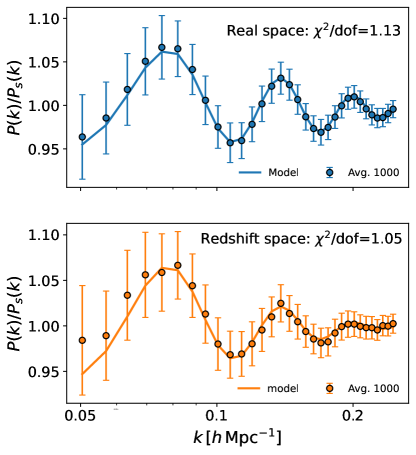
Figure 3: Results of the BAO fitting from the 3D Ly$\alpha$ forest power spectrum. This figure displays the ratio between the full Ly$\alpha$ forest power spectrum and the smooth component, corrected for the nonlinear transfer function $F_{\rm nl}$, in real (top) and redshift space (bottom). The data points are the average power spectrum from $1000$ simulations, the error bars indicate the uncertainties as computed from the diagonal element of the covariance matrix, and the solid line indicates the best-fit model. We also report the $\chi^{2}/$dof in the top right corner of each panel.

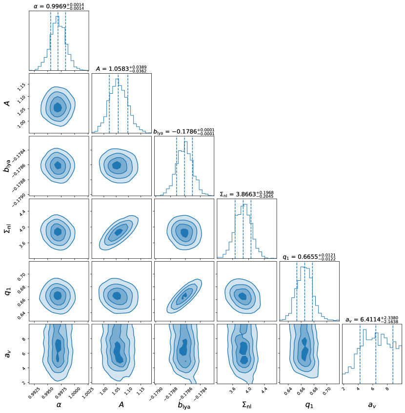
Figure 4: Posterior distributions of the model parameters in real space, obtained via Markov Chains Monte Carlo.

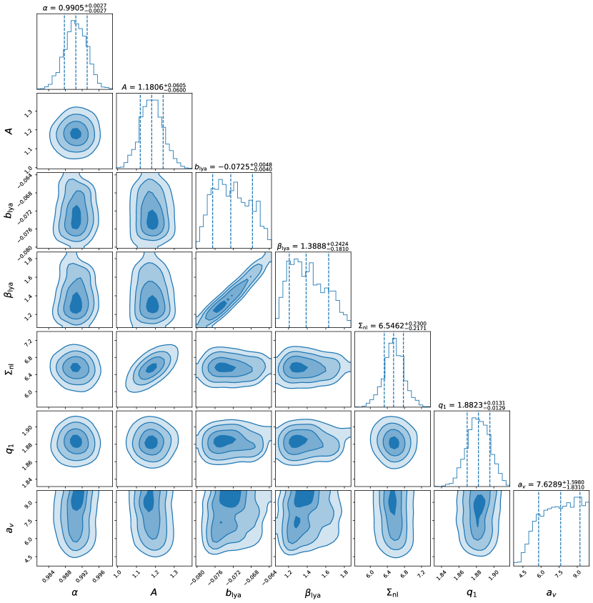
Figure 5: Posterior distributions of the model parameters in redshift space, obtained via Markov Chains Monte Carlo.

To develop an analytical understanding of the findings obtained in this work, we rely on the Lagrangian displacement formalism presented in Eisenstein et al. (2007b). In particular, one can adopt the Zel’dovich approximation (Zel’dovich, 1970) to test the hypothesis that the BAO of the Ly$\alpha$ forest features a negative shift of the acoustic scale.

Let us consider two positions in Lagrangian space $\vec{q}_{1}$ and $\vec{q}_{2}$ and compute their pairwise displacement $\vec{\Psi}_{12}$ projected along the initial separation vector $\vec{r}_{12}=\vec{q}_{1}-\vec{q}_{2}$:

$$\Psi_{12,\parallel}=\frac{\vec{\Psi}_{12}\cdot\vec{r}_{12}}{r_{12}}=\int\frac{d\vec{k}}{(2\pi)^{3}}\,\delta_{\vec{k}}\,\frac{\vec{k}\cdot\vec{r}_{12}}{ik^{2}r_{12}}\,\left(e^{i\vec{k}\cdot\vec{q}_{1}}-e^{i\vec{k}\cdot\vec{q}_{2}}\right)\,.$$ (7)

This quantity tells what is the relative displacement of tracers under the action of gravity.

Let us now define and compute the mean displacement of cosmological tracers (e.g. galaxies) weighted by overdensity pairs:

$$\Psi^{p}_{\parallel}=\frac{\braket{\Psi_{12,\parallel},\delta_{\rm{t},1}\,\delta_{\rm{t},2}}}{{\braket{\delta_{\rm{t},1}\,\delta_{\rm{t},2}}}}\,,$$ (8)

where $\delta_{\rm{t},i}$ is the Lagrangian tracers overdensity field at position $\vec{q}_{i}$, ${\braket{\delta_{\rm{t},1}\,\delta_{\rm{t},2}}}=\xi_{\rm t}(r_{12})$ is the correlation function. Notice that this quantity expresses the mean displacement weighted by the relative contribution to the correlation function. Also, we can express $\delta_{\rm t}$ as a function of $\delta$ using a bias relation $\delta_{\rm t}=\mathcal{B}(\delta)$. Here, we assume a simple linear bias $\delta_{\rm t}=b\delta$ as we are interested in first-order effects, and we assume the bias to be just local, even though the bias could be arbitrarily nonlocal and the calculation would not change to leading order as nonlocal effects are higher-order effects (e.g. McDonald & Roy, 2009). Eventually, as pointed out by Eisenstein et al. (2007b), the stochastic bias interpretation (Dekel & Lahav, 1999) does not change the results, as only $\delta_{\rm t}$ enters in the calculation to leading order when allowing the bias to be a stochastic distribution.

Let us now consider the limit in which the correlation function is much smaller than the variance $|\xi(r_{12})|\ll\sigma^{2}$, where $\sigma^{2}=\braket{\delta^{2}}$, which holds true on sufficiently large scales, relevant for the large-scale linear bias framework we are working with.

Under this assumption and performing all the calculations, one finds:

$$\Psi_{\parallel}^{p}=-\frac{2r_{12}J_{3}(r_{12})}{\sigma}\,\braket{\nu^{2}\nu_{\rm t}(\nu)}\,,$$ (9)

where $J_{3}(r_{12})$ is the integral of the correlation function (Peebles, 1980) and where we have defined the auxiliary variables $\nu=\delta/\sigma$ and $\nu_{\rm t}=\delta_{\rm t}/b\sigma$, i.e. we have rescaled the density fields by their standard deviation.

Eq. 9 clearly shows that a positive linear bias $b>0$ induces a negative pairwise mean Zel’dovich displacement which corresponds — as anticipated above — to a positive shift of the acoustic scale when $\delta_{\rm t}>0$, as happens in the case of galaxies tracing dense environments.

It is well-known that the linear bias $b_{\rm lya}$ of the Ly$\alpha$ forest must assume negative values, because the forest anti-correlates with the dark matter density field (see e.g. du Mas des Bourboux et al., 2020, for an observational measurement of this value from eBOSS). One can also easily show this by means of the FGPA considering that $F=\exp(-\tau)$ and $\tau\sim(1+\delta)^{\gamma}$, which to linear order yields $F\propto-\delta$. For the Ly$\alpha$ forest, the condition $\delta_{\rm t}>0$ — i.e. the regime which dominates the clustering — is typically met in underdense or just mildly overdense regions, where the FGPA holds especially true, as the gas is not shock-heated (e.g. Lukić et al., 2015).

Therefore, while computing the exact value for the shift goes beyond the scope of the paper and would inadequately neglect higher orders beyond linear, this simple argument can be used to provide a justification of the found negative shift ($\alpha-1$) parameter.

6 Conclusions

In this work, we have presented the first quantitative study of the Ly$\alpha$ forest BAO shift from cosmological simulations. In particular, we generated $1000$ $V=(1\,h^{-1}\,{\rm Gpc})^{3}$ fast accurate Ly$\alpha$ forest simulations at $z=2$. We first obtained the dark matter field using the ALPT structure formation model (Kitaura & Hess, 2013), and then applied the nonlocal FGPA prescription (Sinigaglia et al., 2024) to paint the Ly$\alpha$ forest onto the dark matter fields. The free parameters of the nonlocal FGPA were calibrated in such a way to reproduce the 3D power spectrum of the Ly$\alpha$ forest from two fixed-and-paired full cosmological hydrodynamic simulations of volume $V=(500\,h^{-1}\,{\rm Mpc})^{3}$.

We report $\alpha=0.9969^{+0.0014}_{-0.0014}$ in real space, and $\alpha=0.9905^{+0.0027}_{-0.0027}$ in redshift space, i.e., a negative shift of the BAO peak with respect to linear theory at a significance of $\sim 2.2\sigma$ and $\sim 3.5\sigma$, respectively. These findings are in agreement with the picture of an environmental dependence of the BAO shift emerging from the field of galaxy clustering. Moreover, we have shown that this result is also qualitatively consistent with perturbation theory predictions from a simple argument based on the Zel’dovich approximation.

We conclude that this work sets new important theoretical constraints on the Ly$\alpha$ forest BAO scale and offers a potential solution to the tension emerging from previous observational analysis, in an exquisitely timely manner given the unprecedented precision achieved in the recent analysis from DESI Year 1 data (DESI Collaboration et al., 2024b) and its relevance in the global cosmological analysis performed in combination with the data from galaxy clustering measurements (DESI Collaboration et al., 2024c).

References

- Abel et al. (2012) Abel, T., Hahn, O., & Kaehler, R. 2012, MNRAS, 427, 61, doi: 10.1111/j.1365-2966.2012.21754.x
- Achitouv & Blake (2015) Achitouv, I., & Blake, C. 2015, Phys. Rev. D, 92, 083523, doi: 10.1103/PhysRevD.92.083523
- Amendola et al. (2018) Amendola, L., Appleby, S., Avgoustidis, A., et al. 2018, Living Reviews in Relativity, 21, 2, doi: 10.1007/s41114-017-0010-3
- Anderson et al. (2012) Anderson, L., Aubourg, E., Bailey, S., et al. 2012, MNRAS, 427, 3435, doi: 10.1111/j.1365-2966.2012.22066.x
- Angulo & Pontzen (2016) Angulo, R. E., & Pontzen, A. 2016, MNRAS, 462, L1, doi: 10.1093/mnrasl/slw098
- Aoyama et al. (2018) Aoyama, S., Hou, K.-C., Hirashita, H., Nagamine, K., & Shimizu, I. 2018, Monthly Notices of the Royal Astronomical Society, 478, 4905, doi: 10.1093/mnras/sty1431
- Arinyo-i-Prats et al. (2015) Arinyo-i-Prats, A., Miralda-Escudé, J., Viel, M., & Cen, R. 2015, J. Cosmology Astropart. Phys, 2015, 017, doi: 10.1088/1475-7516/2015/12/017
- Bautista et al. (2017) Bautista, J. E., Busca, N. G., Guy, J., et al. 2017, A&A, 603, A12, doi: 10.1051/0004-6361/201730533
- Beutler et al. (2011) Beutler, F., Blake, C., Colless, M., et al. 2011, MNRAS, 416, 3017, doi: 10.1111/j.1365-2966.2011.19250.x
- Beutler et al. (2017) Beutler, F., Seo, H.-J., Ross, A. J., et al. 2017, MNRAS, 464, 3409, doi: 10.1093/mnras/stw2373
- Bi (1993) Bi, H. 1993, ApJ, 405, 479, doi: 10.1086/172380
- Blake & Glazebrook (2003) Blake, C., & Glazebrook, K. 2003, ApJ, 594, 665, doi: 10.1086/376983
- Blas et al. (2011) Blas, D., Lesgourgues, J., & Tram, T. 2011, J. Cosmology Astropart. Phys, 2011, 034, doi: 10.1088/1475-7516/2011/07/034
- Busca et al. (2013) Busca, N. G., Delubac, T., Rich, J., et al. 2013, A&A, 552, A96, doi: 10.1051/0004-6361/201220724
- Chen et al. (2021) Chen, S.-F., Vlah, Z., & White, M. 2021, arXiv e-prints, arXiv:2103.13498. https://arxiv.org/abs/2103.13498
- Cole et al. (2005) Cole, S., Percival, W. J., Peacock, J. A., et al. 2005, MNRAS, 362, 505, doi: 10.1111/j.1365-2966.2005.09318.x
- Croft et al. (1998) Croft, R. A. C., Weinberg, D. H., Katz, N., & Hernquist, L. 1998, in Large Scale Structure: Tracks and Traces, ed. V. Mueller, S. Gottloeber, J. P. Muecket, & J. Wambsganss, 69–75. https://arxiv.org/abs/astro-ph/9801255
- Dekel & Lahav (1999) Dekel, A., & Lahav, O. 1999, ApJ, 520, 24, doi: 10.1086/307428
- Delubac et al. (2015) Delubac, T., Bautista, J. E., Busca, N. G., et al. 2015, A&A, 574, A59, doi: 10.1051/0004-6361/201423969
- DESI Collaboration et al. (2024a) DESI Collaboration, Adame, A. G., Aguilar, J., et al. 2024a, arXiv e-prints, arXiv:2404.03000, doi: 10.48550/arXiv.2404.03000
- DESI Collaboration et al. (2024b) —. 2024b, arXiv e-prints, arXiv:2404.03001, doi: 10.48550/arXiv.2404.03001
- DESI Collaboration et al. (2024c) —. 2024c, arXiv e-prints, arXiv:2404.03002, doi: 10.48550/arXiv.2404.03002
- du Mas des Bourboux et al. (2020) du Mas des Bourboux, H., Rich, J., Font-Ribera, A., et al. 2020, ApJ, 901, 153, doi: 10.3847/1538-4357/abb085
- Eisenstein et al. (2007a) Eisenstein, D. J., Seo, H.-J., Sirko, E., & Spergel, D. N. 2007a, ApJ, 664, 675, doi: 10.1086/518712
- Eisenstein et al. (2007b) Eisenstein, D. J., Seo, H.-J., & White, M. 2007b, ApJ, 664, 660, doi: 10.1086/518755
- Eisenstein et al. (2005) Eisenstein, D. J., Zehavi, I., Hogg, D. W., et al. 2005, ApJ, 633, 560, doi: 10.1086/466512
- Font-Ribera et al. (2014) Font-Ribera, A., Kirkby, D., Busca, N., et al. 2014, J. Cosmology Astropart. Phys, 2014, 027, doi: 10.1088/1475-7516/2014/05/027
- Haardt & Madau (2012) Haardt, F., & Madau, P. 2012, The Astrophysical Journal, 746, 125, doi: 10.1088/0004-637x/746/2/125
- Hadzhiyska et al. (2023) Hadzhiyska, B., Font-Ribera, A., Cuceu, A., et al. 2023, MNRAS, 524, 1008, doi: 10.1093/mnras/stad1920
- Hahn et al. (2007) Hahn, O., Porciani, C., Carollo, C. M., & Dekel, A. 2007, Monthly Notices of the Royal Astronomical Society, 375, 489, doi: 10.1111/j.1365-2966.2006.11318.x
- Hahn et al. (2021) Hahn, O., Rampf, C., & Uhlemann, C. 2021, MNRAS, 503, 426, doi: 10.1093/mnras/staa3773
- Hernández-Aguayo et al. (2020) Hernández-Aguayo, C., Cautun, M., Smith, A., Baugh, C. M., & Li, B. 2020, MNRAS, 494, 3120, doi: 10.1093/mnras/staa973
- Hockney & Eastwood (1981) Hockney, R. W., & Eastwood, J. W. 1981, Computer Simulation Using Particles
- Hopkins et al. (2013) Hopkins, P. F., Narayanan, D., Murray, N., & Quataert, E. 2013, Monthly Notices of the Royal Astronomical Society, 433, 69, doi: 10.1093/mnras/stt688
- Hui et al. (1997) Hui, L., Gnedin, N. Y., & Zhang, Y. 1997, ApJ, 486, 599, doi: 10.1086/304539
- Kaiser (1984) Kaiser, N. 1984, ApJ, 284, L9, doi: 10.1086/184341
- Kitaura et al. (2022) Kitaura, F. S., Balaguera-Antolínez, A., Sinigaglia, F., & Pellejero-Ibáñez, M. 2022, MNRAS, 512, 2245, doi: 10.1093/mnras/stac671
- Kitaura & Hess (2013) Kitaura, F. S., & Hess, S. 2013, MNRAS, 435, L78, doi: 10.1093/mnrasl/slt101
- Kitaura et al. (2016) Kitaura, F.-S., Chuang, C.-H., Liang, Y., et al. 2016, Phys. Rev. Lett., 116, 171301, doi: 10.1103/PhysRevLett.116.171301
- Levi et al. (2013) Levi, M., Bebek, C., Beers, T., et al. 2013, arXiv e-prints, arXiv:1308.0847. https://arxiv.org/abs/1308.0847
- Lewis & Challinor (2011) Lewis, A., & Challinor, A. 2011, CAMB: Code for Anisotropies in the Microwave Background, Astrophysics Source Code Library, record ascl:1102.026
- Lukić et al. (2015) Lukić, Z., Stark, C. W., Nugent, P., et al. 2015, MNRAS, 446, 3697, doi: 10.1093/mnras/stu2377
- McDonald & Roy (2009) McDonald, P., & Roy, A. 2009, Journal of Cosmology and Astroparticle Physics, 2009, 020–020, doi: 10.1088/1475-7516/2009/08/020
- Nagamine et al. (2021) Nagamine, K., Shimizu, I., Fujita, K., et al. 2021, ApJ, 914, 66, doi: 10.3847/1538-4357/abfa16
- Neyrinck et al. (2018) Neyrinck, M. C., Szapudi, I., McCullagh, N., et al. 2018, MNRAS, 478, 2495, doi: 10.1093/mnras/sty1074
- Peebles (1980) Peebles, P. J. E. 1980, The large-scale structure of the universe
- Peebles & Yu (1970) Peebles, P. J. E., & Yu, J. T. 1970, ApJ, 162, 815, doi: 10.1086/150713
- Planck Collaboration et al. (2020) Planck Collaboration, Aghanim, N., Akrami, Y., et al. 2020, A&A, 641, A6, doi: 10.1051/0004-6361/201833910
- Prada et al. (2016) Prada, F., Scóccola, C. G., Chuang, C.-H., et al. 2016, MNRAS, 458, 613, doi: 10.1093/mnras/stw312
- Saitoh (2017) Saitoh, T. R. 2017, AJ, 153, 85, doi: 10.3847/1538-3881/153/2/85
- Saitoh & Makino (2009) Saitoh, T. R., & Makino, J. 2009, ApJ, 697, L99, doi: 10.1088/0004-637X/697/2/L99
- Saitoh & Makino (2013) Saitoh, T. R., & Makino, J. 2013, The Astrophysical Journal, 768, 44, doi: 10.1088/0004-637x/768/1/44
- Schmittfull et al. (2015) Schmittfull, M., Feng, Y., Beutler, F., Sherwin, B., & Chu, M. Y. 2015, Phys. Rev. D, 92, 123522, doi: 10.1103/PhysRevD.92.123522
- Seljak (2012) Seljak, U. 2012, J. Cosmology Astropart. Phys, 2012, 004, doi: 10.1088/1475-7516/2012/03/004
- Seo & Eisenstein (2003) Seo, H.-J., & Eisenstein, D. J. 2003, ApJ, 598, 720, doi: 10.1086/379122
- Sherwin & Zaldarriaga (2012) Sherwin, B. D., & Zaldarriaga, M. 2012, Phys. Rev. D, 85, 103523, doi: 10.1103/PhysRevD.85.103523
- Shimizu et al. (2019) Shimizu, I., Todoroki, K., Yajima, H., & Nagamine, K. 2019, Monthly Notices of the Royal Astronomical Society, 484, 2632, doi: 10.1093/mnras/stz098
- Sinigaglia et al. (2021) Sinigaglia, F., Kitaura, F.-S., Balaguera-Antolínez, A., et al. 2021, ApJ, 921, 66, doi: 10.3847/1538-4357/ac158b
- Sinigaglia et al. (2022) —. 2022, ApJ, 927, 230, doi: 10.3847/1538-4357/ac5112
- Sinigaglia et al. (2024) Sinigaglia, F., Kitaura, F. S., Nagamine, K., Oku, Y., & Balaguera-Antolínez, A. 2024, A&A, 682, A21, doi: 10.1051/0004-6361/202346931
- Slosar et al. (2013) Slosar, A., Iršič, V., Kirkby, D., et al. 2013, J. Cosmology Astropart. Phys, 2013, 026, doi: 10.1088/1475-7516/2013/04/026
- Smith et al. (2017) Smith, B. D., Bryan, G. L., Glover, S. C. O., et al. 2017, MNRAS, 466, 2217, doi: 10.1093/mnras/stw3291
- Springel (2005) Springel, V. 2005, Monthly Notices of the Royal Astronomical Society, 364, 1105, doi: 10.1111/j.1365-2966.2005.09655.x
- Sunyaev & Zeldovich (1970) Sunyaev, R. A., & Zeldovich, Y. B. 1970, Ap&SS, 7, 3, doi: 10.1007/BF00653471
- Werner & Porciani (2020) Werner, K. F., & Porciani, C. 2020, MNRAS, 492, 1614, doi: 10.1093/mnras/stz3469
- White et al. (2010) White, M., Pope, A., Carlson, J., et al. 2010, ApJ, 713, 383, doi: 10.1088/0004-637X/713/1/383
- Zel’dovich (1970) Zel’dovich, Y. B. 1970, A&A, 5, 84
- Zhao et al. (2022) Zhao, C., Variu, A., He, M., et al. 2022, MNRAS, 511, 5492, doi: 10.1093/mnras/stac390