Robust Affine Formation Control
of Multiagent Systems
Abstract
Affine formation control is a subset of formation control methods, which has gained increasing popularity for its flexibility and maneuverability in diverse applications. Affine formation control is inherently distributed in nature, where the local controllers onboard each agent are linearly dependent on the relative position measurements of the neighboring agents. The unavailability of these measurements in practice, due to node failure or missing links, leads to a change in the underlying graph topology, and subsequently causes instability and sub-optimal performance. In this paper, we propose an estimation framework to enhance the robustness of distributed affine formation control systems against these topology changes. Our estimation framework features an adaptive fusion of both temporal information from the dynamics of agents and spatial information which is derived from the geometry of the affine formations. We propose a suite of algorithms under this framework to tackle various practical scenarios, and numerically verify our proposed estimator on stability, convergence rate, and optimality criterion. Simulations show the performance of our proposed algorithms as compared to the state-of-the-art methods, and we summarize them with future research directions.
Index Terms:
distributed filtering, affine formation control, Kalman filtering, relative localization, time-varying graphs.I Introduction
Multiagent systems have been widely researched for their broad applications in various fields such as artificial intelligence [2], swarm robotics [3], social networks [4], and space applications [5]. Various swarm applications require agents to collectively preserve a geometric pattern, i.e., a formation such as collective object transport [6], space-based interferometry [7], or various sensing missions [8]. It relies on measurements of relative information among agents to achieve different formations. For instance, distance measurements are used to achieve rigid formations that allow translations and rotations [9, 10], bearing measurements allow formations with scaling of the geometry [11, 12], and displacements can be employed to realize affine formations [13].
Affine formation control is a subset of general formation control, where the positions of the agents are restricted to affine transformations over time, which include, but are not limited to rotation, translation, and shearing. Since their introduction in 2016 [13], affine formation control has evolved in various directions and has been put into practice [14]. For instance, an extension is made in [15] from shape control to a maneuver control scenario which means the agents are expected to track a time-varying target configuration with a continuously changing geometry. The underlying graph is also extended to a directed topology [16, 17]. The modeling of agents is generalized from single- and double-integrator agents to more general agents in [18]. The maneuverability of affine formations is achieved by setting a small subset of agents as leaders, whose positions are known. In using a hierarchical control approach for the leaders [19], special cases of affine transformation can be realized. Recent works also show that some maneuvers can be achieved by modifying the stress matrix [20, 21] without the need for leaders. Apart from the controller designs, distributed filtering is also developed and applied to yield more optimal implementations in noisy environments [22]. In general, affine formation control has a relatively simple controller design, but its stability relies on the rigidity of the underlying framework which can be demanding in practice.
Distributed Affine formation control, inherently relies on relative position information of neighborhood nodes, which needs to be measured and communicated. Any failure of the sensing or the communication in practice will change the underlying graph topology, which may cause stability and optimality issues. In networked and distributed control literature, this problem can be modeled as either a switching topology or packet dropouts. For switching topology, state-of-the-art solutions often model the possible topologies and predevelop stabilizing controllers for each [23, 24, 25]. This approach usually implies that the system is stabilizable under each topology such that a controller can be designed among other practical considerations. However, this condition is too restrictive for affine formation control due to the rigidity requirements [13]. Also, switching topology typically does not deal with scenarios where the departures of agents do not affect the formation of the others. On the other hand, packet dropouts, which model an intermittent behavior for the observations [26, 27], can be addressed by estimating the missing information on a fixed topology. This type of method relies on estimator designs but can simplify the problem on the control end. If the estimation is sufficiently accurate, the system exhibits the same closed-loop stability and optimality. For instance, [28] employed long short-term memory to predict the position of the leaders in the event of packet losses. Other common approaches include Kalman filtering to predict the missing information based on the dynamic models [29]. However, these methods are not designed for permanent information loss, e.g., a departing node. In general, there lacks a unified approach to tackle all potential topological changes for affine formation control.
I-A Contributions
In this work, we propose a generic distributed estimation framework in discrete time for robust affine formation control. We model the topology changes as the observation losses or edge unavailability, which are then estimated using our proposed observation model. We propose a fusion of temporal and spatial information in the framework, which enable a wide range of practical scenarios to be tackled, including random and permanent observation losses and node departures. Our main contributions are as follows.
-
•
We propose an observation model of relative positions that accounts for the noises introduced in the measurements and their unavailabilities.
-
•
We adopt the Kalman filters in a relative state-space model to address intermittent losses, which is named relative Kalman filtering (RKF). We also propose an estimator using the geometry of affine formations, which we call relative affine localization (RAL), and also propose an improved variant that adopts a dynamic consensus i.e., consensus RAL (conRAL). Our proposed framework that fuses RKF and RAL is called geometry-aware Kalman filtering (GA-RKF).
-
•
In our fusion framework, we propose a key adaptive indicator that locally approximates the system convergence, and show this adaptive indicator is mathematically bounded by the tracking error, the common global convergence indicator.
Layout: In Section II, the preliminaries of affine formation control are introduced and the representation of topology changes is modeled as a time-varying functional graph. In Section III, we motivate the need to model partial observations and give the observation model in a state-space form. In Section IV, we discuss the geometry estimator design in detail and options for improvements. The local convergence indicator, which plays a critical role in adaptive fusion is introduced in Section V followed by some algorithms designs under the proposed framework in Section VI. Numerical validations to test our proposed algorithms are performed in Section VII and followed by conclusions and future works.
Notation: Vectors and matrices are represented by lowercase and uppercase boldface letters respectively such as and . The elements of matrix are expressed using where and denote the index of rows and columns, respectively. Sets and graphs are represented using calligraphic letters e.g., , and the intersection and union of sets are and , respectively. The relative complement of two sets is denoted by \. Vectors of length of all ones and zeros are denoted by and , respectively. An identity matrix of size is denoted by . The Kronecker product is and a vectorization of a matrix is denoted by by stacking all the columns vertically. The trace operator is denoted by . We also use subscripts on vectors and matrices to indicate a time-varying variable.
II Preliminaries
II-A Graph Theory
We consider a setup where mobile agents work in -dimensional space with typically being or . The underlying connections of the agents are described by an undirected nominal graph where the set of vertices is and the set of edges is . As an undirected graph is equivalent to a bidirectional graph, i.e., , we assume there are directed edges (or undirected edges) in total. The set of neighbors of a node is defined as , and the corresponding cardinality is denoted by with . The time-varying functional graph that represents the actual connectivity of the system is where is the discrete-time subscript. It is a subgraph of the nominal graph where the vertex set and the edge set are both subsets of those in the nominal graph, i.e., and . As such, there are nodes in the functional graph. Similarly, the time-varying cardinality of the set of neighbors is denoted by with .
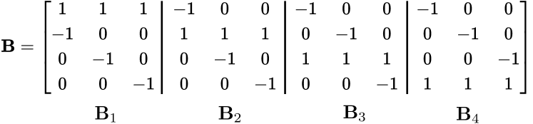
In this work, we frequently use the incidence matrix of a graph. For the functional graph, the bidirectional incidence matrix is defined by
| (1) |
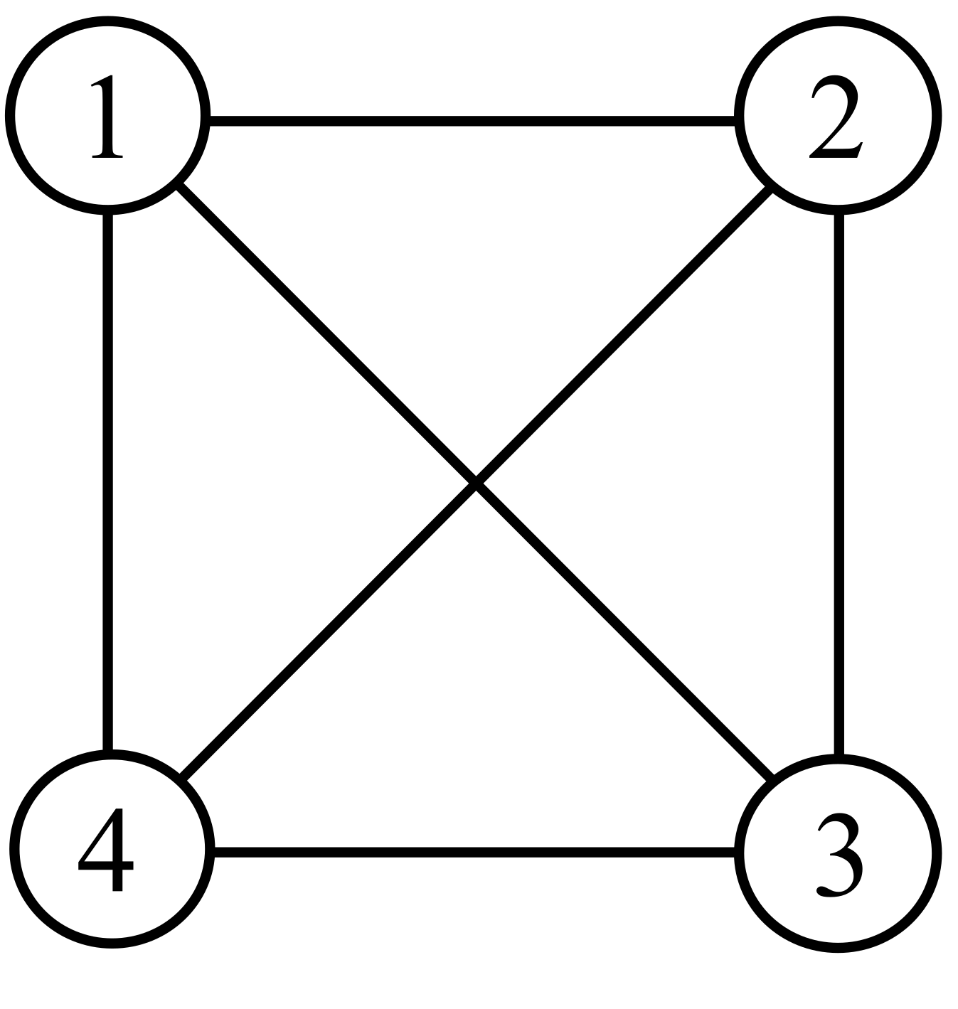
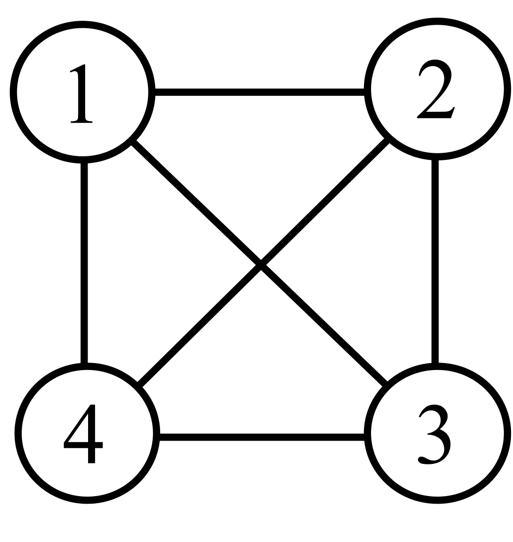
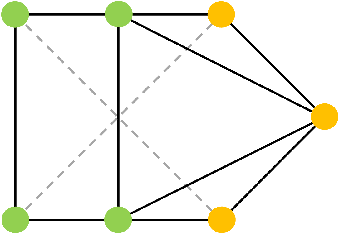
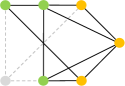
which admits the structure where the matrix , group the columns per agent. As an example, the incidence matrix of the nominal graph shown in Fig. 1 can be found in Fig. 2, and the time-varying for the functional graph collects a subset of the columns from each block based on edge availability.
II-B Geometric Transformations
We define as the time-varying position of agent at time instant , and collect all the positions of the agents in a configuration matrix . Similarly, a target configuration that collects the expected positions of agents is defined as in which is the individual target position for each agent . For the nominal graph , we introduce a nominal configuration where is the nominal position for agent . The nominal configuration represents a general geometric pattern the agents are expected to achieve, and the time-varying target configuration is a continuous mapping from the nominal configuration to the target configuration through geometric transformations. We associate the nominal graph and the nominal configuration by a nominal framework . A summary of the notations on the configurations is presented in Table I.
| config. | notation () | local rep. () | description |
|---|---|---|---|
| nominal | fixed, s.t. design | ||
| target | mapped by (2) | ||
| real-time | s.t. control |
In the context of affine formation control, the transformation is limited to affine transformations which are characterized by a transformation matrix and a translation vector , where the superscript indicates a mapping for target configurations, which is subject to planning. The target configuration is then defined in global form by
| (2) |
or from a local view of the th agent , we have
| (3) |
From a geometric perspective, an affine transformation can be considered as a combination of basic geometric transformations including translation, scaling, rotation, and shearing, as shown in Fig. 1. In practice, certain geometric transformations and their combinations are special cases of affine transformation, which are widely applied in various scenarios. Correspondingly, the transformation matrix is constrained to specific structures, and the degrees of freedom are reduced compared to general affine transformations. These properties will be explored in subsequent sections.
II-C Formation Control Laws
The goal of formation control is to reach a desired geometric pattern [13], and maneuver control enables the agents to navigate in space with continuously changing geometric patterns [15]. The maneuverability is typically ensured by a technique called leader-follower strategy in which a small set of agents are set aside to be the leaders and the rest are the followers. The time-varying target formation is prescribed to the leaders while the followers only need to follow the leaders and stay in formation without any knowledge of the target configurations. In this work, we focus on the followers in the leader-follower approach as the leaders typically occupy a small portion of the nodes and are thus considered trivial.
Controller design regarding affine formation control are abundant in literature for different agent dynamics. For simplicity, we limit our discussion to single-integrator controllers i.e., in a continuous form where is the velocity input, however our proposed approach can be applied, in general to any displacement-based controllers that depend on relative positions up to a translation. The discrete-time version of single-integrator dynamics is
| (4) |
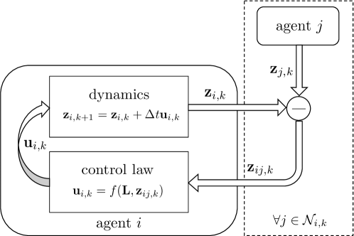
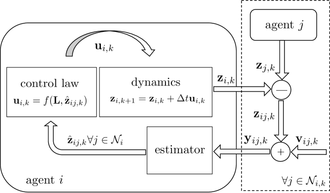
where agents’ positions are updated by the control input in a short time interval . Some control input designs are shown in Table II, where in the table is the relative position up to a translation at time instance which are modeled as the edges of the graph. Also, are elements of the stress matrix whose computation can be found in [13] and [15]. A diagram to illustrate the interactions in a formation control system is shown in Fig. 3. Following the control laws the agents can converge to and track the target positions from a random initialization.
II-D Assumptions
We now make the following assumptions on the network for establishing stability.
| Leaders | Control law |
|---|---|
| static | |
| constant velocity | |
| varying velocity |
Assumption 1 (Communication graph and measurement graph).
We assume that the communication graph is the same as the measurement graph, i.e., no communication is established if the edge is unavailable in the functional graph.
This assumption is reasonable because the unavailability of observations is typically due to unreliable wireless channels in many cases as a large portion of relative localization methods are typically based on radio frequency signals [30].
Assumption 2 (Stabilizability of an undirected framework).
The nominal framework is universally rigid such that the formation control system is stabilizable [13].
Assumption 2 has direct implications and conditions on the stress matrix used in the controller designs, which indicates the existence of a stabilizing controller.
III Problem Formulation
III-A Motivation for Modeling Partial Observations
In the previous section, we emphasized the need for Assumption 2 for the stabilization of the existing controllers under undirected nominal graphs, which may not be readily satisfied by a network in reality. The cause for these situations usually involves communication constraints, e.g., bandwidth, communication radius, and sensor scheduling or malfunctioning. A few scenarios are discussed below and illustrated in Fig. 4.
III-A1 Directed functional graphs
Since functional graphs are subgraphs of the undirected nominal graph, there can be cases where information flows only one way. In this case, pair is a directed edge and the functional graph is a directed realization, as shown in Fig. 4(b). The controllers designed for directed topology cannot be applied in this case this issue can happen randomly and unexpectedly.
III-A2 Violation of stabilizing conditions
III-A3 Departing and rejoining agents
A common practical case is where agents, due to maintenance, trajectory constraints, etc., cannot maintain the formation but have to temporarily or permanently depart from the swarm as shown in Fig. 4(d). This occurs frequently with satellites in space applications. In this case, the rest of the agents are still expected to maintain the formation until the same agent or its replacement returns or for the rest of the task.
III-B Data Model
In this section, we provide an overview and modeling of the proposed framework in which we aim to estimate relative positions up to a translation for . We first introduce general local relative (or edge) state-space modeling with the state variable for which includes the relative positions and relevant higher-order kinematics such as (relative) velocities and accelerations although for single-integrator controllers only relative positions are of primary concern. The state-space model adopts the form
| (5a) | ||||
| (5b) | ||||
where is the state transition matrix designed based on the assumed dynamics, is the selection matrix that maps full state variable to observations of relative positions, and and are assumed to be zero-mean Gaussian. Note that, the dynamics in (5) provide the possibilities for standard tracking models such as constant acceleration, etc, and adaptive tracking algorithms, e.g., Kalman filters, can be used for estimation or prediction.
We now propose the following observation model to incorporate partial observations,
| (6) |
where
| (7) |
is the observation available to agent with noise , and is an estimate using the geometry of formation if the observation cannot be made. This estimate is Gaussian with covariance where is the resulting covariance from a geometrical estimation and is our proposed novel adaptive penalty on the uncertainty reflecting the quality of , which is discussed in detail later. As such, the observation-covariance pair in the observation model (6) is either or based on the availability of observation. An overview of the system architecture with partial observation and estimation is shown in Fig. 5 compared to the ideal case in Fig. 3. Next, we provide more details on , the estimation using the geometry of the formation.
IV Estimation from Geometry
The intuition behind geometric estimation is that the configuration space spanned by the positions of agents is mapped from a much smaller space described by the geometric parameters and . Similar insights also hold for relative positions, thus they can be estimated by reconstructing the geometry parameters using part of the observed relative positions for the neighbors. We show that the relative positions are only dependent on the transformation matrix which can be estimated using a simple least-square formulation. Then the unobserved relative positions can be reconstructed using the estimated . This method is named relative affine localization (RAL) which has necessary conditions on the nominal configuration and the functional graph which can be violated in practice. We also propose techniques to relax these conditions and produce more accurate estimations by exploiting the geometry of formation or using neighborhood communication.
IV-A Relative Affine Localization
We first assume the case where the formation reaches sufficient convergence, i.e., for and introduce the geometer estimation. In later sections, we discuss the modeling of sufficiency of convergence. Observe that
| (8) |
where comes from the known nominal configuration. This means that the target relative positions are linear to and so is upon sufficient convergence. From model (7), the observations can be written as which, by aggregating all available observations, leads to
| (9) |
where collects noiseless relative positions , collects the corresponding relative nominal positions , and is the noise matrix from . An estimation of the geometric parameters can be obtained by
| (10) |
where . The geometric estimates can be subsequently obtained by
| (11) |
with a covariance structure
| (12) |
where is the noise covariance for available observations from model (7), and this expression for is derived in Appendix A. A unique solution using (11) is guaranteed if is full row rank, which translates to some geometric conditions which we refer to as geometric feasibility.


Remark 1 (Geometric feasibility for RAL).
Estimator (10) is geometrically feasible if and only if contains at least observations of neighboring agents that are not collinear in or coplanar in in the nominal configuration.
Some examples are given in Fig. 6 to explain this feasibility further. As , geometric feasibility can be decomposed into necessary conditions of and : configuration is generic [13] and meaning has at least columns. Another intuitive understanding of geometrical feasibility for RAL is the minimum number of independent equations to solve for the parameters in the underlying affine transformation.
Although geometric feasibility can be achieved in various scenarios, it can still be violated in loosely connected networks. To overcome this limitation, we introduce two approaches to relax the geometric feasibility for the broader applicability of the geometric estimator and more optimal estimations.
| Scaling | Rotation | Similarity | |
|---|---|---|---|
| constraints | is diagonal | ||
| solutions |
IV-B Constrained RAL
The first approach is when special cases of affine transformation are adopted and known to the agents. In practice, some maneuvers require specific transformations such as scaling only, rotation or similarity transforms. In these cases, the affine transformation matrix admits to a particular structure or presents some properties. By leveraging constraints on the formulation (10) the inversion in the solution to (10) can be avoided and thus the geometric feasibility is relaxed. An overview of these constrained problems and their solutions are shown in Table III, which are discussed in detail in the following. Using these constraints, the geometric feasibility is relaxed to observation in the neighborhood for both and .
Scaling. Scaling is an important feature of affine transformation that allows the swarm to pass through narrow passages or obstacles. For cases where only scaling is involved in the affine transformation, the parameter matrix degenerates to
| (13) |
where , for , scales each dimension. Since the diagonality of decouples the dimensions, the problem could be decomposed into independent least squares problems and estimates for can be easily given.
Rotation. Rotation is a form of Euclidean transform that preserves the rigidity of the formation. It allows a collective change of orientation of the formation. The parameter matrix in this case is a rotation matrix that is orthonormal as shown in Table III. This formulation is recognized as the orthogonal Procrustes problem [31] where an orthogonal matrix is sought to approximate rotations between two body frames. There are numerical and analytical solutions [32] available, and we adopt a singular value decomposition (SVD) based solution from [33].
Similarity. In similarity transforms all dimensions are uniformly scaled by a non-negative on top of a rotation. Hence, the constraints on can be relaxed from to , which then results in the formulation in Table III. The estimation can be based on the rotation estimation from the rotation case with an additional estimation on the scalar. If and both have economy-sized SVD with and as the respective diagonal matrices, the scalar can be estimated by dividing the energies on each (rotated) dimension before and after transformation.
IV-C Consensus Filtering
Another approach to relax geometric feasibility is to use the estimated from neighbors. In essence, the geometry parameters can be considered latent parameters which are estimated by RAL using a consensus process. As such, distributed filtering and fusion across the network can also be applied in the latent space for two purposes: reducing the noise of the estimated and sharing the estimates in case geometric feasibility is violated. We propose the use of a well-established dynamic consensus filtering protocol as follows [34]:
| (14) |
where are estimates from RAL and is a known small value. Here, is the union set of the neighbors and node , i.e., .
V Local Convergence Indicator
In the previous section we assumed the formation has sufficiently converged i.e., for , to derive the geometrical estimators, however, this is not assumed to be the case upon the initialization of the configuration. Similar scenarios could also occur when large environmental disturbances, e.g., gusts, temporarily deform the converged configuration. Therefore, the geometric estimators may not be accurate until the system converges, which is why our proposed model (6) introduces an adaptive penalty for the covariance of the geometric estimates to account for the error and is a local convergence indicator (CI) to gauge the sufficiency of convergence.
An ideal indicator function would be the tracking error
| (15) |
which is commonly used in literature to indicate convergence and steady-state error [15, 17, 35, 36]. However, this is a global function by nature and thus is locally intractable. In addition, neither the absolute positions in nor the target configuration are assumed to be known to the follower agents, which makes it infeasible to calculate. We therefore propose the following CI
| (16) |
where is a local estimate of the geometry parameters using (10), and shall be accessible through neighborhood communication. In contrast to (15), our proposed CI (16) requires no global information but exhibits a similar trend as the tracking error . Intuitively, this function measures the difference between the estimates of the geometry parameters. If the system has converged to an affine formation, these estimates shall reach a consensus, which is illustrated in Fig. 7. In the following theorem and corollary, we show the relationship between and , which leads to a claim on the convergence guarantees CI.
Theorem 1 (Upper bound of the convergence indicator).
Proof. See Appendix B-A
Theorem 1 shows, that if the tracking error asymptotically and exponentially converges to zero under some control protocols, the local indicator will also converge similarly up to a known scalar. In the noisy case, it can be intuitively speculated that similar conclusions hold for the expectation of the functions, which is formalized in the following.
Corollary 1 (Upper bound of CI under observation noises).
Under observation model (9), the expectation of the local convergence indicator is upper bounded by the expectation of the tracking error up to a scaling factor and an offset, i.e, , where
| (18a) | ||||
| (18b) | ||||
Proof. See Appendix B-B.
When noise is present, a biased term related to the covariance of the noise appears in the inequality. In this case, we claim that if the noise energy is finite and the tracking error is converging to zero, CI also converges to a finite value.
It should be noted from the definition of CI (16) only requires agreement on the estimated parameter matrix in the neighborhood to reach zero. This means for any configuration up to an affine transformation. For instance, if the system converges to the target configuration up to a large translation, indicators for all will be zero but the tracking error will be large, which makes the convergence for a sufficient but not necessary condition for the convergence as described. As such, CI should be generally considered a shape convergence indicator rather than a maneuver indicator. In practice, as the setting of leaders will ensure convergence of target configuration, we can use to locally refer to global convergence.
VI Algorithms
We now summarize our proposed solution, which is a fusion of temporal information using a Kalman filter and spatial information from the geometry of the affine formation in a general form, and it constitutes the ”estimator” block in Fig. 5. In summary, we present 3 algorithms, relative Kalman filtering (RKF), relative affine localization (RAL) with consensus filtering (conRAL), and geometry-aware RKF (GA-RKF), which can all be derived from model (5) and (6).
VI-A Case 1: Relative Kalman Filtering
We first discuss the relative state-space model (5), where we consider a constant acceleration model. The matrices in (5) are then
| (19) | |||||
| (20) | |||||
| (21) |
where is the variance of acceleration uncertainty, which can be further tuned. The covariance structure can be derived by projecting small deflections of acceleration in the state vector. Algorithm 1 describes the proposed relative Kalman filter (RKF), which is a direct adaptation of the Kalman filtering under intermittent observations [37] to our relative state-space model (5) for affine formation control. It propagates the dynamic model to predict without correction from the observations if they are unavailable.
This algorithm, as we will show in the simulation section, is robust to random losses of observations since the dynamic model can capture some motion information of the agent and predictions can be made when necessary. In practice, relative state-space modeling can also be done using other models or combinations of models such as interactive multiple models (IMM) for better approximation.
VI-B Case 2: RAL with Consensus Filtering
Similar to the Kalman filtering, RAL-based algorithms can also be stand-alone estimators. Here we introduce an improved version that concatenates RAL with the consensus filtering protocol, which mitigates the constraint of geometric feasibility, in scenarios when estimators may not exist due to insufficient observations.
In Algorithm 2, if the algorithm does not execute consensus filtering and simply adopt , a standard RAL is performed. In addition, if geometric feasibility does not hold but the system is adopting special cases of affine transformations and is known as prior knowledge, the computation of can be done using solutions from Table III instead. The performance of this algorithm depends on the quality of the estimation of and is particularly useful in case of node departures. In these cases, the neighboring agents will estimate the missing edges as if they are still active.
VI-C Case 3: Geometry-Aware Kalman Filtering
Algorithm 3 gives the details of the fusion of RAL-based algorithms and RKF. Using the full proposed framework, RAL estimates are computed first, which can be treated as alternative observations for unavailable edges for the Kalman filter. The consensus indicators are also computed prior to the filtering step, which is then used to weigh the uncertainty of the RAL estimates. Note that, the Algorithm 3 reduces to Algorithm 1 if RAL cannot be performed due to geometric feasibility.
VII Simulations
In this section, we present numerical validations of several practical scenarios to show the enhanced robustness of using our proposed algorithms.
VII-A Simulation Setup
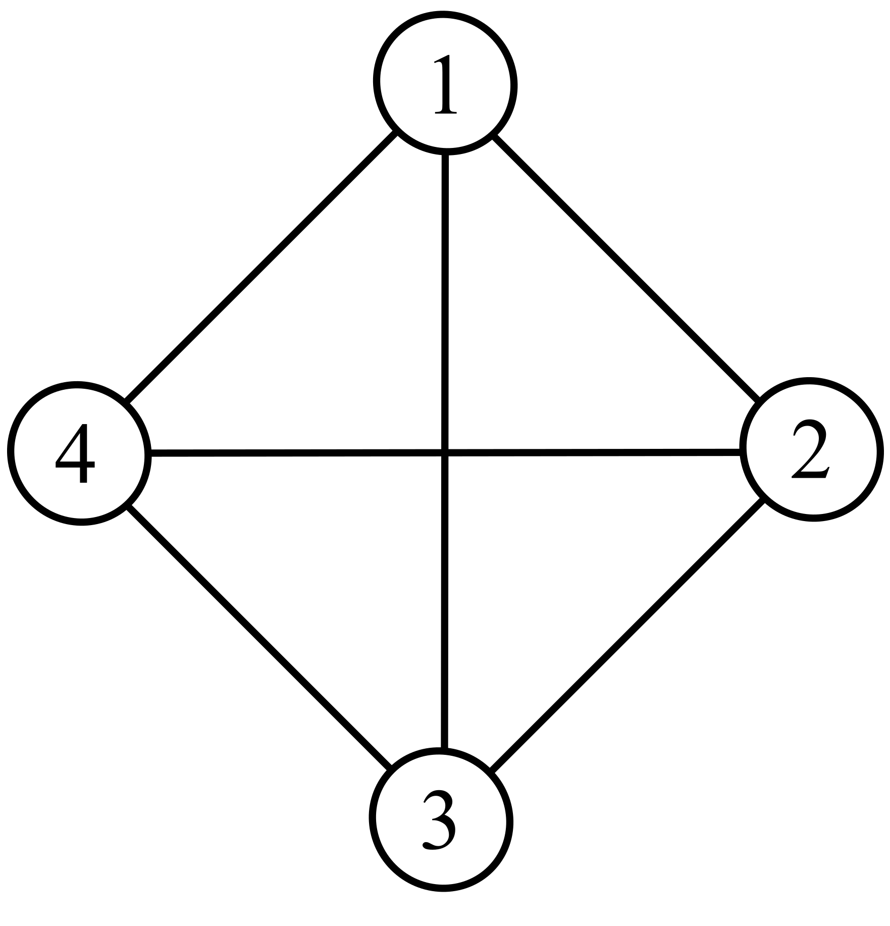
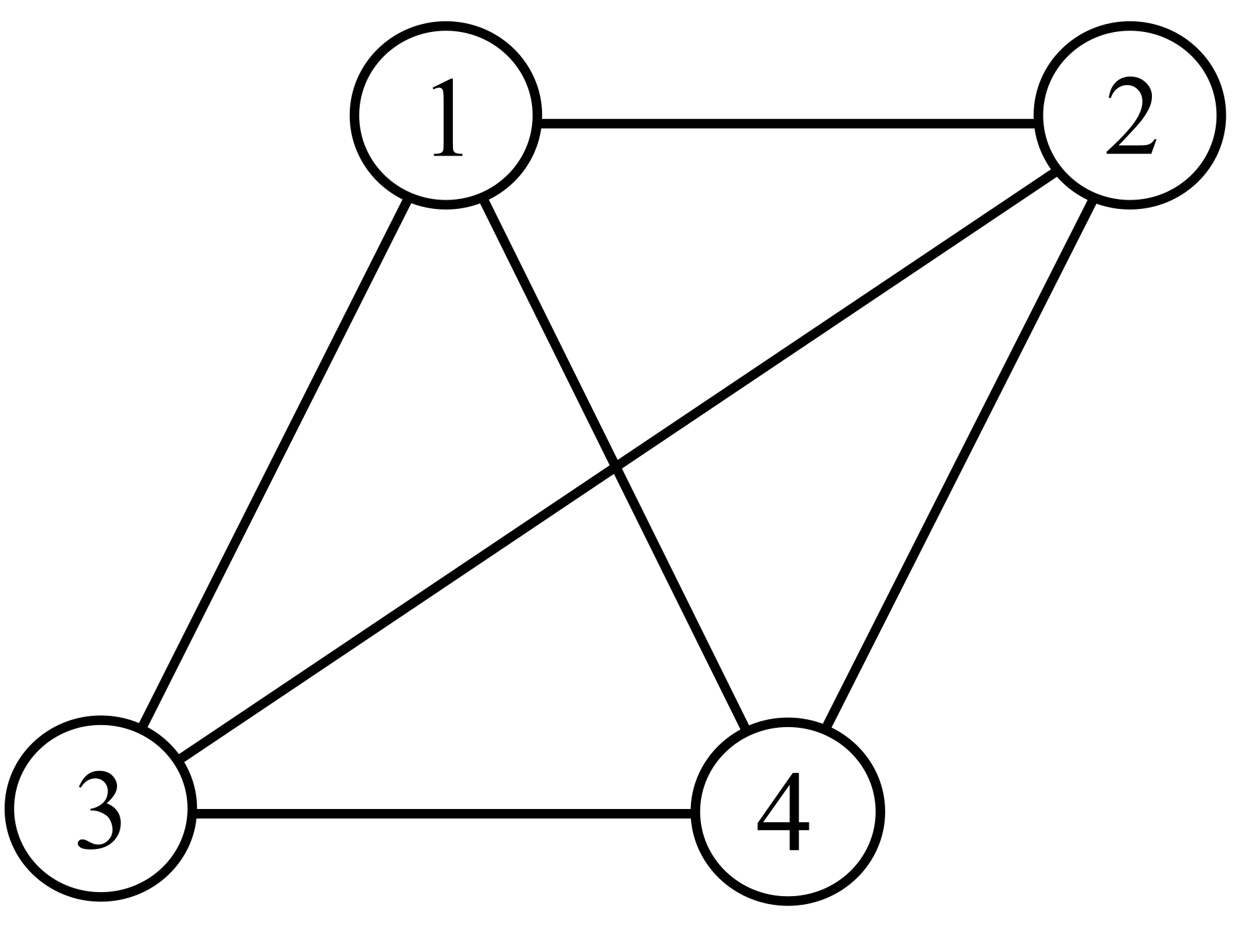
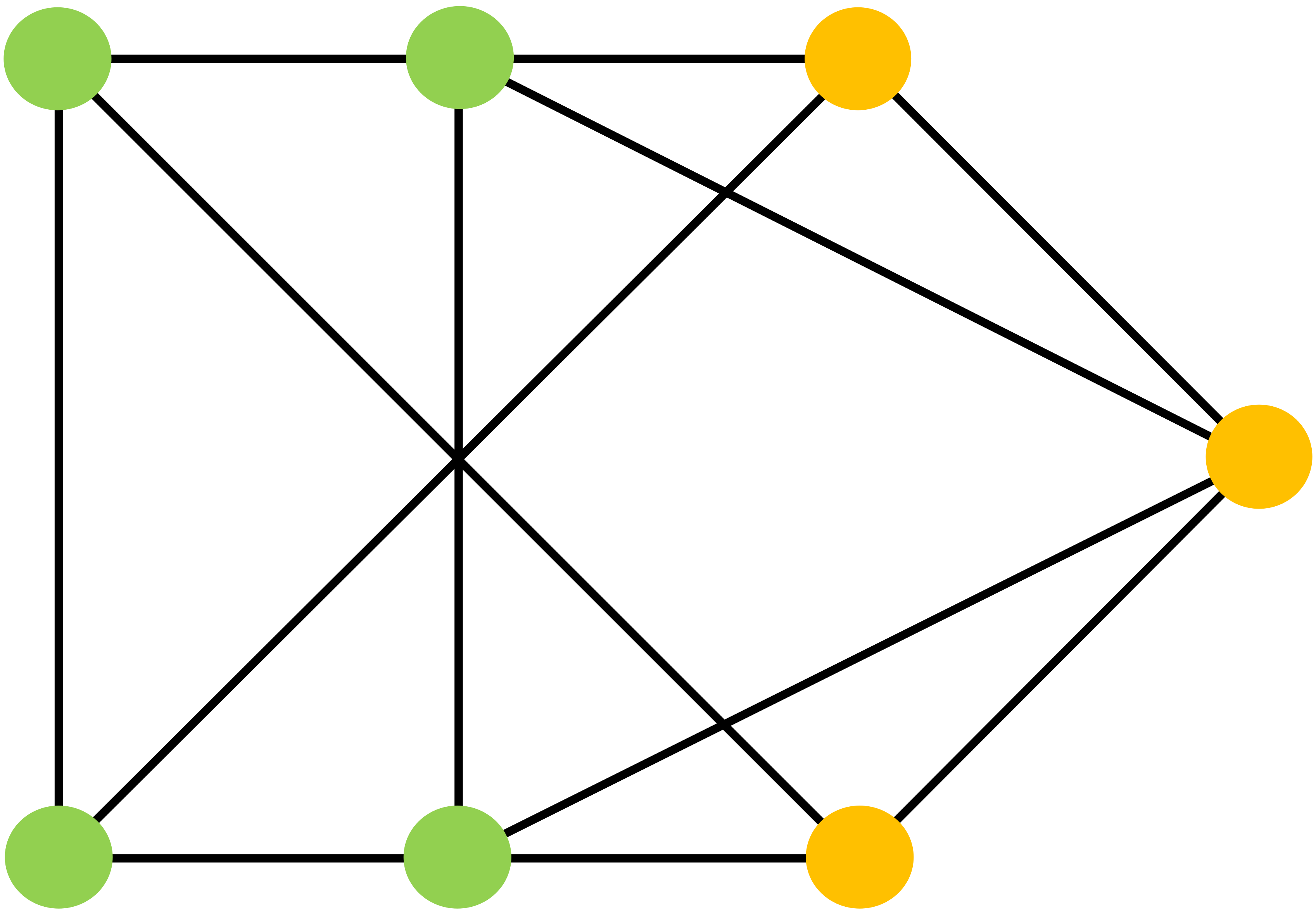
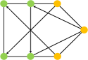
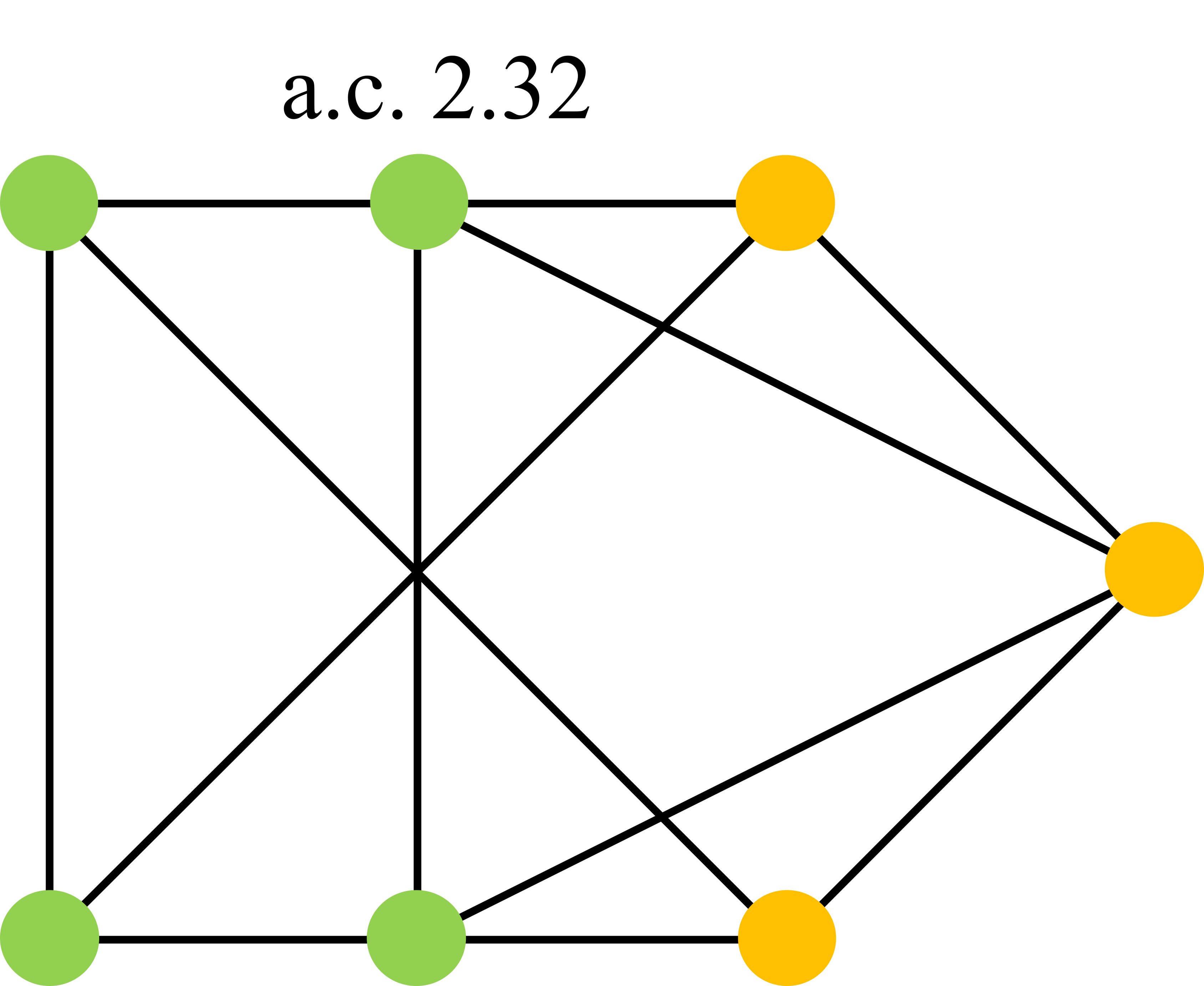
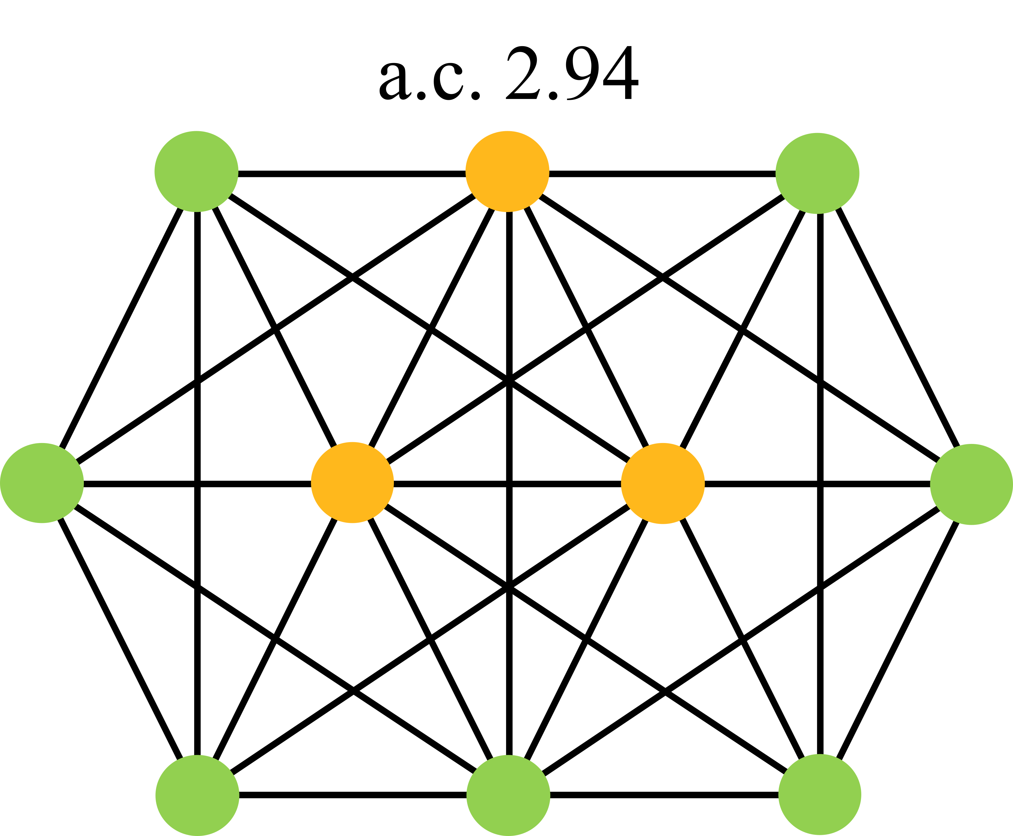
We consider two formations in Fig. 9 presented in the literature [1, 15]. Graph 1 has nodes with undirected edges and Graph 2 has nodes with undirected edges. They are selected for the simulations as they feature different densities of connections indicated by algebraic connectivity (a.c.). The more sparsely connected formations are considered more susceptible to being unstabilizable under time-varying functional graphs with loss of information. We intend to show that our proposed algorithms work for both formations.
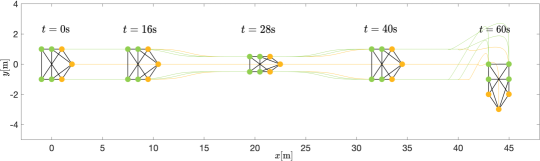
The maneuvering pattern used in the simulation is shown in Fig. 8 where the duration of the simulation is and the time step is chosen as meaning discrete time instances in total. For all the results on the tracking error (15), Monte Carlo simulations are run for each discrete time instance and averaged over the number of simulations, unless otherwise indicated. The noise covariance for the observation model (7) is chosen as a constant where is selected as .
VII-B Convergence Indicator
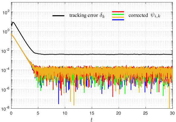
In Section V, we showed that the convergence indicator (16) is upper bounded by the tracking error (15) through Theorem 1 and Corollary 1. We first show the result of the convergence indicator in Fig. 10. Here, we present the tracking error in black and the convergence of CI for each follower in color using Graph 1. To give a direct comparison, the CIs are corrected with their corresponding coefficients and which are time-invariant in this example as we use nominal graphs with any observation losses. As can be seen from the figure, the corrected CI is always upper-bounded by the tracking error which substantiates Corollary 1. Another observation from Fig. 10 is that the CI follows the tracking error which makes it a reasonable local approximator. In the case of time-varying graphs, the variance of CI could be larger than shown in Fig. 10, but remains upper bounded to the tracking error.
VII-C Random Observation Losses
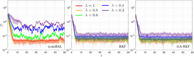
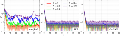
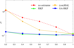
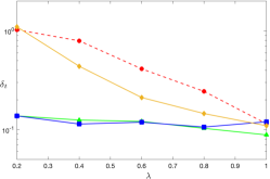
If the observation loss occurs randomly, we model its availability using a Bernoulli distribution with probability . Larger values of indicate fewer losses on average for each edge over time. means the functional graphs are the same as the nominal graph and no edge losses are present. The proposed algorithms for both graphs in Fig. 9 with different choices of are shown in Fig. 11 where the convergence of Algorithm 1-3 is shown. Two focuses should be made w.r.t these convergence curves: one is the steady-state error and the other is the convergence speed. In general, the larger is, the more available edges, thus the better performance in both convergence speed and steady-state error. Compared to using only geometry information in Algorithm 1 (conRAL), RKF-based algorithms are more capable of dealing with low observation availabilities with a convergence speed nearly the same as the case. This can be also verified in Fig. 12 (a) and (b) where the mean tracking error ( averaged across the duration of simulation) is compared for the algorithms across different choices of . It can be seen that the curves for RKF and GA-RKF are almost flat across meaning that they are strongly robust to random losses of observations whereas conRAL deteriorates to the no estimator case as gets smaller.
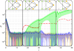
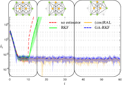
VII-D Switching Topologies with Node Departures
We show a few topology switching cases for both nominal graphs as shown in Fig. 12 (c) and (d). Here, we test the ability of our proposed estimators to maintain stability. As can be seen, the ”no estimator” case and RKF diverge with topology change whereas conRAL and GA-RKF maintain the convergence. The reason for the divergence of ”no estimator” is that the underlying graph changes result in different stress matrices for the controller and the new stress matrices do not necessarily exist due to the rigidity requirement. For the RKF, the predictions are outdated as soon as the relative dynamics change without the correction of observations. As such, a simple maneuver of the systems can cause instability. On the other hand, since the geometry estimation is still accurate as the edge losses and node departures do not instantly corrupt the geometric pattern, our proposed estimators conRAL and GA-RKF can maintain the converged state. Therefore, they are considered robust to switching topologies, as compared to RKF.
VIII Conclusion
In this paper, we proposed an estimation framework to enhance the robustness of affine formation control to the loss of observations which are modeled as time-varying functional graphs. Our framework fuses estimators using both temporal and spatial (geometrical) information and is also flexible to exploit these estimators individually. Some example algorithms are presented under the proposed framework and we presented simulations for different types of time-varying graphs. In particular, the geometry-aware relative Kalman filtering (GA-RKF) is proven to be robust for all presented scenarios. In our future work, we aim to further strengthen several aspects of our proposed framework. First, the discussions are limited to the edges availability and node departures w.r.t. followers. Furthermore, theoretical guarantees on the stability of the formation control using such an estimation framework should be investigated.
References
- [1] Z. Li and R. T. Rajan, “Geometry-aware distributed kalman filtering for affine formation control under observation losses,” in 2023 26th International Conference on Information Fusion (FUSION), 2023, pp. 1–7.
- [2] A. Heuillet, F. Couthouis, and N. Díaz-Rodríguez, “Collective explainable ai: Explaining cooperative strategies and agent contribution in multiagent reinforcement learning with shapley values,” IEEE Computational Intelligence Magazine, vol. 17, no. 1, pp. 59–71, 2022.
- [3] Y. Rizk, M. Awad, and E. W. Tunstel, “Cooperative heterogeneous multi-robot systems: A survey,” ACM Computing Surveys (CSUR), vol. 52, no. 2, pp. 1–31, 2019.
- [4] R. Ureña, G. Kou, Y. Dong, F. Chiclana, and E. Herrera-Viedma, “A review on trust propagation and opinion dynamics in social networks and group decision making frameworks,” Information Sciences, vol. 478, pp. 461–475, 2019. [Online]. Available: https://www.sciencedirect.com/science/article/pii/S0020025518309253
- [5] G. Zhao, H. Cui, and C. Hua, “Hybrid event-triggered bipartite consensus control of multiagent systems and application to satellite formation,” IEEE Transactions on Automation Science and Engineering, vol. 20, no. 3, pp. 1760–1771, 2023.
- [6] J. Alonso-Mora, S. Baker, and D. Rus, “Multi-robot formation control and object transport in dynamic environments via constrained optimization,” The International Journal of Robotics Research, vol. 36, no. 9, pp. 1000–1021, 2017. [Online]. Available: https://doi.org/10.1177/0278364917719333
- [7] G.-P. Liu and S. Zhang, “A survey on formation control of small satellites,” Proceedings of the IEEE, vol. 106, no. 3, pp. 440–457, 2018.
- [8] K. A. Ghamry and Y. Zhang, “Cooperative control of multiple uavs for forest fire monitoring and detection,” in 2016 12th IEEE/ASME International Conference on Mechatronic and Embedded Systems and Applications (MESA), 2016, pp. 1–6.
- [9] S.-M. Kang, M.-C. Park, B.-H. Lee, and H.-S. Ahn, “Distance-based formation control with a single moving leader,” in 2014 American Control Conference, 2014, pp. 305–310.
- [10] D. Van Vu, M. H. Trinh, P. D. Nguyen, and H.-S. Ahn, “Distance-based formation control with bounded disturbances,” IEEE Control Systems Letters, vol. 5, no. 2, pp. 451–456, 2021.
- [11] S. Zhao and D. Zelazo, “Translational and scaling formation maneuver control via a bearing-based approach,” IEEE Transactions on Control of Network Systems, vol. 4, no. 3, pp. 429–438, 2017.
- [12] J. Zhao, X. Li, X. Yu, and H. Wang, “Finite-time cooperative control for bearing-defined leader-following formation of multiple double-integrators,” IEEE Transactions on Cybernetics, vol. 52, no. 12, pp. 13 363–13 372, 2022.
- [13] Z. Lin, L. Wang, Z. Chen, M. Fu, and Z. Han, “Necessary and sufficient graphical conditions for affine formation control,” IEEE Transactions on Automatic Control, vol. 61, no. 10, pp. 2877–2891, 2016.
- [14] P. Zhang, D. Ma, P. Liu, and M. Li, “Robust affine maneuver formation control based of second-order multi-agent grid inspection systems,” Frontiers in Energy Research, vol. 10, 2022. [Online]. Available: https://www.frontiersin.org/articles/10.3389/fenrg.2022.972999
- [15] S. Zhao, “Affine formation maneuver control of multiagent systems,” IEEE Transactions on Automatic Control, vol. 63, no. 12, pp. 4140–4155, 2018.
- [16] L. Wang, Z. Lin, and M. Fu, “Affine formation of multi-agent systems over directed graphs,” in 53rd IEEE Conference on Decision and Control, 2014, pp. 3017–3022.
- [17] Y. Xu, S. Zhao, D. Luo, and Y. You, “Affine formation maneuver control of multi-agent systems with directed interaction graphs,” in 2018 37th Chinese Control Conference (CCC), 2018, pp. 4563–4568.
- [18] ——, “Affine formation maneuver control of linear multi-agent systems with undirected interaction graphs,” in 2018 IEEE Conference on Decision and Control (CDC), 2018, pp. 502–507.
- [19] Y. Lin, Z. Lin, Z. Sun, and B. D. O. Anderson, “A unified approach for finite-time global stabilization of affine, rigid, and translational formation,” IEEE Transactions on Automatic Control, vol. 67, no. 4, pp. 1869–1881, 2022.
- [20] H. G. de Marina, J. Jimenez Castellanos, and W. Yao, “Leaderless collective motions in affine formation control,” in 2021 60th IEEE Conference on Decision and Control (CDC), 2021, pp. 6433–6438.
- [21] C. Garanayak and D. Mukherjee, “Leaderless affine formation maneuvers over directed graphs,” in 2022 IEEE 61st Conference on Decision and Control (CDC), 2022, pp. 3983–3988.
- [22] M. Van Der Marel and R. T. Rajan, “Distributed kalman filters for relative formation control of multi-agent systems,” in 2022 30th European Signal Processing Conference (EUSIPCO), 2022, pp. 1422–1426.
- [23] T. Han, Z. Lin, R. Zheng, and M. Fu, “A barycentric coordinate-based approach to formation control under directed and switching sensing graphs,” IEEE Transactions on Cybernetics, vol. 48, no. 4, pp. 1202–1215, 2018.
- [24] X. Dong and G. Hu, “Time-varying formation control for general linear multi-agent systems with switching directed topologies,” Automatica, vol. 73, pp. 47–55, 2016. [Online]. Available: https://www.sciencedirect.com/science/article/pii/S0005109816302515
- [25] Z. Wang, T. Liu, and Z.-P. Jiang, “Cooperative formation control under switching topology: An experimental case study in multirotors,” IEEE Transactions on Cybernetics, vol. 51, no. 12, pp. 6141–6153, 2021.
- [26] G. Franzè, A. Casavola, D. Famularo, and W. Lucia, “Distributed receding horizon control of constrained networked leader–follower formations subject to packet dropouts,” IEEE Transactions on Control Systems Technology, vol. 26, no. 5, pp. 1798–1809, 2018.
- [27] X. Gong, Y.-J. Pan, J.-N. Li, and H. Su, “Leader following consensus for multi-agent systems with stochastic packet dropout,” in 2013 10th IEEE International Conference on Control and Automation (ICCA), 2013, pp. 1160–1165.
- [28] L. Sedghi, J. John, M. Noor-A-Rahim, and D. Pesch, “Formation control of automated guided vehicles in the presence of packet loss,” Sensors, vol. 22, no. 9, 2022. [Online]. Available: https://www.mdpi.com/1424-8220/22/9/3552
- [29] J. Lee, S.-Y. Park, D.-E. Kang et al., “Relative navigation with intermittent laser-based measurement for spacecraft formation flying,” Journal of Astronomy and Space Sciences, vol. 35, no. 3, pp. 163–173, 2018.
- [30] S. Chen, D. Yin, and Y. Niu, “A survey of robot swarms′ relative localization method,” Sensors, vol. 22, no. 12, 2022. [Online]. Available: https://www.mdpi.com/1424-8220/22/12/4424
- [31] S. Prince, Computer Vision: Models Learning and Inference. Cambridge University Press, 2012.
- [32] T. Viklands, “Algorithms for the weighted orthogonal procrustes problem and other least squares problems,” Ph.D. dissertation, Datavetenskap, 2006. [Online]. Available: https://api.semanticscholar.org/CorpusID:6919969
- [33] P. H. Schönemann, “A generalized solution of the orthogonal procrustes problem,” Psychometrika, vol. 31, pp. 1–10, 1966. [Online]. Available: https://api.semanticscholar.org/CorpusID:121676935
- [34] R. Olfati-Saber and J. Shamma, “Consensus filters for sensor networks and distributed sensor fusion,” in Proceedings of the 44th IEEE Conference on Decision and Control, 2005, pp. 6698–6703.
- [35] H. Su, Z. Yang, S. Zhu, and C. Chen, “Bearing-based formation maneuver control of leader-follower multi-agent systems,” IEEE Control Systems Letters, vol. 7, pp. 1554–1559, 2023.
- [36] F. Xiao, Q. Yang, X. Zhao, and H. Fang, “A framework for optimized topology design and leader selection in affine formation control,” IEEE Robotics and Automation Letters, vol. 7, no. 4, pp. 8627–8634, 2022.
- [37] B. Sinopoli, L. Schenato, M. Franceschetti, K. Poolla, M. Jordan, and S. Sastry, “Kalman filtering with intermittent observations,” IEEE Transactions on Automatic Control, vol. 49, no. 9, pp. 1453–1464, 2004.
- [38] K. B. Petersen, M. S. Pedersen et al., “The matrix cookbook,” Technical University of Denmark, vol. 7, no. 15, p. 510, 2008.
Appendix A Derivation of the covariance for (12)
Appendix B Convergence Indicator
B-A Proof of Theorem 1
B-B Proof of Corollary 1
| (25a) | ||||
| (25b) | ||||
| (25c) | ||||
| (25d) |
where the expressions for , and are given in (26).
| (26a) | ||||
| (26b) | ||||
| (26c) | ||||
We first define the expectation of the tracking error as
| (27) |
and the expectation of CI is
| (28) |
and we analyze each term individually. Since is the same as (24c), we can directly rewrite
| (29a) | ||||
| (29b) | ||||
For term in (26),
| (31a) | ||||
| (31b) | ||||
| (31c) | ||||
as the noises in matrices for all and are zero-mean and not correlated with .
B-C Property
Property 1.
Given a matrix where , the following statement holds true
| (35) |